


Abstract
Overparameterized deep neural networks (DNNs) rely heavily on high-quality labels, while conventional cross entropy (CE) tends to overfit incorrect annotations under label noise, leading to degraded generalization performance. Robust loss functions alleviate this issue by reducing sensitivity to noisy labels. However, strict symmetric losses often exhibit limited fitting capability, while full normalization may alter the optimization properties of the original loss. To address these limitations, we propose surprise-annealed dual-tail loss (SADT), a bounded multiclass classification objective constructed from predictive surprise. Specifically, SADT retains the original predictive surprise in the active score construction when the predicted probability is at least the chance level, progressively compresses moderate surprise through an inverse hyperbolic sine branch, and bounds the extreme tail using an arctangent branch. By combining a normalized active score with a log balanced passive score, SADT achieves an exact constant class sum. Theoretically, we establish its boundedness and prove that it preserves clean risk minimizers under uniform symmetric label noise with a corruption rate below (C − 1)/C. For class conditional and instance-dependent noise, we derive conditional robustness guarantees and an excess risk bound. Experiments show that SADT improves accuracy over NCE + NNCE by 2.64% and 3.16% on CIFAR-10 with 80% symmetric noise and WebVision, respectively, while showing weaker performance on Clothing1M. These results demonstrate the effectiveness of SADT under several challenging noise conditions while revealing its limitations in learning from difficult clean samples.
1. Introduction
In recent years, over-parameterized deep neural networks (DNNs) achieve remarkable success in various visual tasks due to their powerful fitting capability [1,2], yet their superior performance largely relies on large-scale data with high-quality annotations. However, obtaining fully reliable human annotations in real-world applications is often costly [3], while commonly used data collection approaches, such as crowdsourcing, web crawling, and large-model-based automatic annotation, inevitably introduce noisy labels [4]. Since DNNs not only learn meaningful patterns from data but also gradually memorize random or incorrect annotations, training with the standard cross entropy (CE) loss typically causes models to first learn relatively simple clean patterns and then progressively fit noisy samples, ultimately degrading generalization performance. Consequently, noisy labels learning (NLL) becomes an important research problem in robust machine learning [5,6,7].
Existing NLL methods mainly mitigate erroneous supervision through sample selection [8,9,10], label correction [11,12,13], and robust loss design [14,15,16]. Among them, robust losses offer an important advantage: they typically require neither additional networks, clean validation sets, nor explicit noise rate prior, and can directly replace standard training objectives or be integrated into other NLL frameworks. Ghosh et al. [5,7] theoretically establish conditions under which a loss function achieves noise tolerance under certain symmetric and asymmetric noise settings. The theories motivate a series of robust losses such as GCE [17] and SCE [18]. However, the strict symmetry condition is inherently restrictive. Although full normalization makes the sum of losses over all classes constant [19,20], it may substantially alter the gradient structure of the original loss and weaken its optimization capability. ALF [14,15] further show that more general noise tolerance under clean label dominant noise can be achieved if the optimal direction of the weighted conditional risk is determined by the class with the largest weight. This result extends robust loss design from enforcing a strict cross-class constant sum condition to controlling the relative optimization advantages among different label terms. Subsequent studies further improve the balance between noise suppression and effective sample fitting through negative learning [16], gradient clipping [21], active and passive asymmetric combinations [22,23], and gradient variation [24]. These studies indicate that an effective robust loss should not only suppress erroneous supervision but also preserve sufficient learning signals from reliable samples.
Despite these advances, robust loss design still faces two key challenges. First, balancing noise suppression and effective learning remains a key challenge in robust loss design. Existing methods typically limit the loss response to low-confidence labels to reduce the influence of noisy supervision. However, low confidence does not necessarily indicate an incorrect label, as hard clean samples may also receive low predicted probabilities. Therefore, excessive loss suppression may weaken informative learning signals. Second, bounded loss responses do not necessarily guarantee strict noise tolerance. Although gradient clipping and loss variation constraints reduce the influence of noisy labels, they do not ensure a constant sum of losses across classes, which is crucial for robustness under symmetric label noise [5]. Full normalization satisfies this condition but may alter optimization behavior across different confidence regions. These challenges motivate two research questions. First, how can a robust loss suppress unreliable supervision without excessively weakening the learning signals from difficult clean samples? Second, how can a loss function maintain effective optimization while satisfying the exact constant class sum condition required for robustness under uniform symmetric label noise?
To address these challenges, we propose surprise-annealed dual-tail loss (SADT) for robust NLL. Specifically, for the first question, SADT introduces a dual-tail transformation and surprise-dependent annealing to regulate loss responses across different confidence regions. To address the second question, SADT combines a normalized active score with a log-balanced passive score, ensuring an exact constant class sum while retaining confidence-dependent loss regulation. Therefore, for an input sample x with observed label , let denote the softmax probability assigned to , and let C be the number of classes. We define the predictive surprisal as t = −logp to quantify the disagreement between the observed label and the model prediction. When p ≥ 1/C, SADT preserves the original surprisal to maintain effective learning. For moderately unlikely labels with 1/C2 ≤ p < 1/C, it progressively contracts the loss response through a class-scaled inverse hyperbolic sine branch. For extremely unlikely labels with p < 1/C2, a continuously joined arctangent branch further bounds the extreme tail. Furthermore, SADT introduces surprisal-dependent annealing weights to smoothly adjust the loss response according to prediction disagreement, suppressing highly unreliable supervision while preserving learning signals from hard clean samples. Both transition points are analytically determined by the number of classes, eliminating the need for additional threshold tuning. To ensure strict robustness under symmetric label noise, SADT further incorporates a loss structure consisting of a normalized active score and a logarithmically balanced passive score. The former preserves relative predictive information across classes, while the latter combines normalized negative evidence with a probability complement term using fixed mixing weights determined solely by the number of classes. This design ensures an exact constant class sum of α + β(C − 1), where α and β control the active and passive components, respectively. Theoretical analysis shows that SADT preserves the global minimizers of the clean risk under uniform symmetric label noise (Sym.) when the noise rate satisfies ρ < (C − 1)/C. For asymmetric (Asym.) and instance-dependent noise (IDN), we further establish sufficient conditions based on clean-class posterior dominance and derive total-variation-based excess risk bounds under general label corruption. The main contributions of this work are summarized as follows:
- We propose SADT, a surprisal-based dual-tail robust loss. It employs the random-guessing level as an analytical boundary and uses inverse hyperbolic sine and arctangent branches to continuously regulate loss responses in low-confidence regions. Surprisal-dependent annealing further suppresses highly unreliable supervision while preserving informative signals from hard samples.
- We integrate the proposed surprise regulation mechanism into a normalized active and log-balanced passive loss structure, maintaining an exact constant class sum while preserving confidence-dependent loss regulation.
- We establish theoretical guarantees under different noisy settings. We prove that SADT preserves the clean-risk minimizers under uniform symmetric noise with a specified noise-rate condition. For asymmetric and instance-dependent noise, we derive sufficient conditions based on posterior dominance and total variation-based excess risk bounds.
- Extensive experiments under synthetic and real-world label noise validate the effectiveness and robustness of the proposed method.
2. Related Works
2.1. Robust Loss Function Research
Robust loss functions reduce the sensitivity of deep neural networks (DNNs) to noisy labels by adjusting the loss response to different predictions. Ghosh et al. [5,7] theoretically investigate the noise tolerance of loss functions and show that a constant sum of losses across all classes preserves risk minimizers under certain symmetric noise conditions. This finding provides an important theoretical foundation for robust loss design. Subsequently, GCE [17] provides a continuous transition between CE and MAE through a tunable parameter, thereby balancing fitting capability and noise robustness and inspiring subsequent robust loss designs. SCE [18] combines CE with reverse CE to improve both learning efficiency and robustness. Ma et al. [19] further normalize general losses into forms satisfying the constant sum condition and derive NCE from CE. Based on their optimization behaviors, they categorize existing robust losses into active and passive losses and combine NCE as the active component with MAE as the passive component to form a joint objective. This design further motivates a series of composite robust losses. For example, ANL [16] combines a normalized active loss with a normalized negative loss, allowing the passive component to extend beyond MAE-type objectives.
However, strict loss symmetry does not necessarily ensure favorable optimization behavior. Full normalization may alter loss responses and gradients across different confidence regions, potentially weakening informative learning signals. To relax the symmetry requirement, Zhou et al. [14,15] introduce asymmetric losses and characterize more general robustness through a condition in which the class with the largest weight determines the optimal direction. JAL [22] extends asymmetric robustness to active and passive loss combinations, while OGC [23] improves noise tolerance through gradient clipping. In contrast, VBL [24] establishes robustness analyses by controlling gradient variation under symmetric and asymmetric noise. Although recent methods have improved robustness through asymmetric loss design and gradient regulation, they do not explicitly combine surprise-dependent loss transformation and annealing to regulate learning signals across different confidence regions. In contrast, SADT introduces a continuous dual-tail transformation with surprise-dependent annealing to progressively suppress extreme surprise while retaining informative responses from relatively reliable samples. Furthermore, its normalized active and log-balanced passive components ensure an exact constant class sum, providing theoretical noise tolerance under uniform symmetric label noise.
2.2. Other NLL Methods
Sample selection and label correction are two other major directions in NLL. Sample selection typically exploits the tendency of deep networks to first learn easy and clean samples and then gradually memorize noisy labels, thereby identifying more reliable samples during training [25,26]. Recent methods also address the erroneous removal of hard clean samples by incorporating confidence trends [27] or debiased selection mechanisms [12], etc. Label correction instead estimates latent clean labels using model predictions, soft labels, or multi-model consistency [28,29]. Existing studies mainly exploit useful supervision from noisy data through dual-model collaboration [30]. Although these approaches often achieve strong performance, they usually rely on sample partitioning, noise prior or additional training stages. In contrast, robust losses neither explicitly identify clean samples nor correct their labels but directly limit the influence of erroneous supervision on risk optimization through loss design, allowing them to be used independently or further integrated with the above LNL frameworks [31,32].
3. Methods
3.1. Problem Formulation
We consider a C-class classification problem. Given the dataset , DNN fθ outputs logits , and the softmax layer produces the prediction
Here, . We denote p = p(xi) = [p1(xi),…,pK(xi)]. For any classification loss L, the clean expected risk is
Let yi denote the latent clean label and denote the observed label which may be noisy (i.e., ). The label noise can be categorized into different types according to how the label corruption probability depends on the input features and the latent clean class, including class-conditional noise (CCN) and instance-dependent noise (IDN). Moreover, CCN consists of uniform noise (symmetric noise) and asymmetric noise. When the label is corrupted, Equation (2) is converted to the noisy risk:
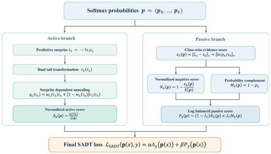
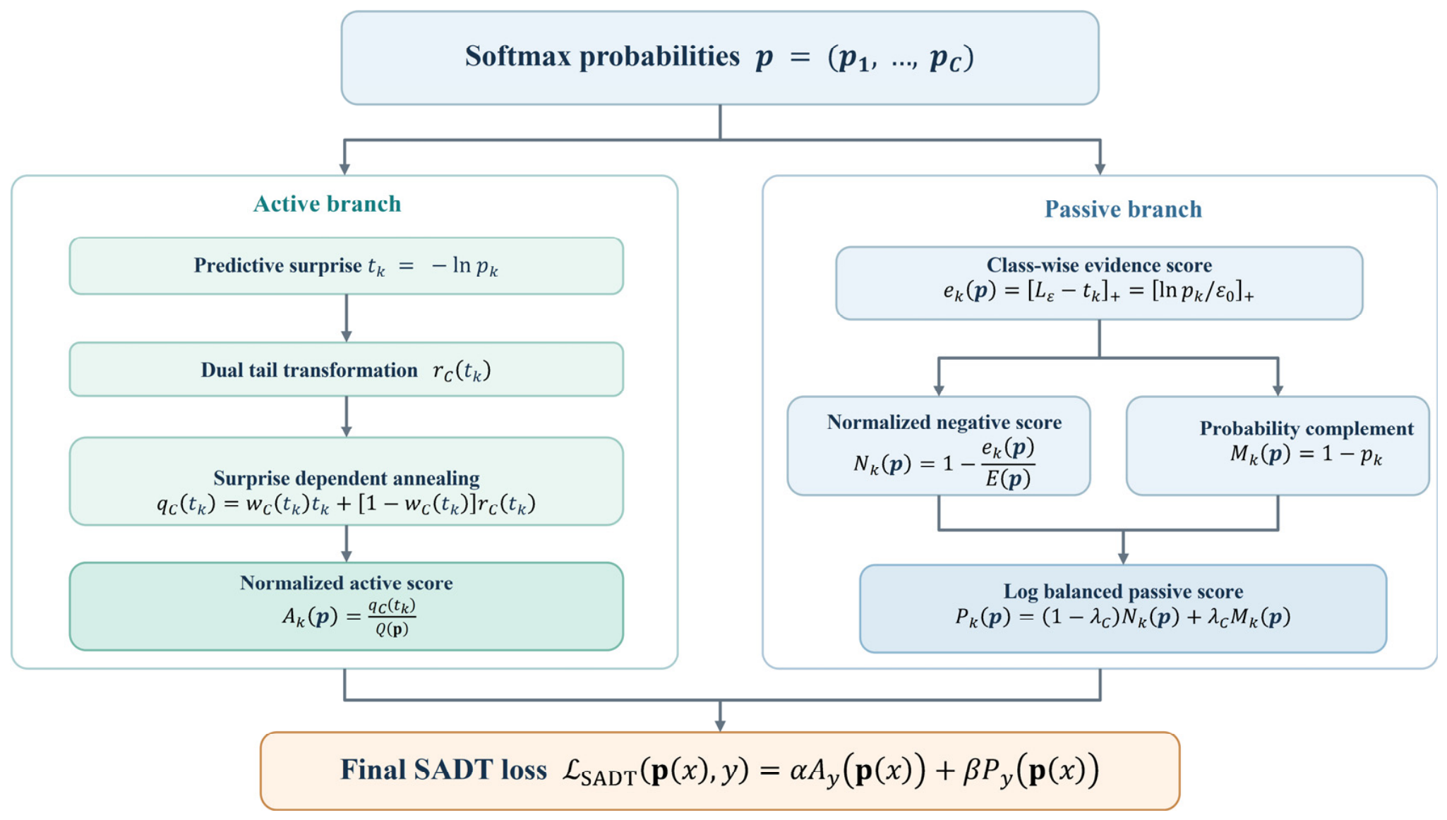
Here, , and η(x) denotes the corrupted and clean class posteriors, respectively, while ρx and ρx,k denote the instance-dependent corruption rate and the corresponding transition probabilities. This notation distinguishes posterior probabilities from label corruption parameters. denotes the noise transition probability. The overall framework of SADT is presented in Figure 1.
Figure 1.
Overall framework of the proposed SADT loss. The active branch regulates predictive surprise through dual-tail transformation and surprise-dependent annealing, while the passive branch combines normalized negative evidence and probability complement. Their weighted combination forms the final SADT objective with an exact constant class sum.
3.2. Surprise-Annealed Dual-Tail Loss
Existing robust losses, such as NCE + NNCE [16], improve noise tolerance by combining normalized active and negative losses. However, these methods do not explicitly distinguish loss responses across different predictive surprise regions. Since low confidence may indicate either an incorrect label or a difficult clean sample, uniformly suppressing low-confidence responses may weaken informative learning signals. To address this limitation, SADT introduces a dual-tail transformation combined with surprise-dependent annealing. Specifically, the dual-tail transformation preserves the original surprise when the predicted probability is at least 1/C, progressively compresses moderate surprise through an inverse hyperbolic sine branch, and bounds extreme surprise using an arctangent branch. Surprise-dependent annealing further adjusts the contribution of the original surprise and its transformed response, allowing smoother regulation across confidence regions. Unlike NCE + NNCE, the main distinction of SADT lies in this joint regulation mechanism, which is incorporated into a normalized active component and combined with a log-balanced passive component to maintain an exact constant class sum. The following sections detail its mathematical construction and theoretical properties.
3.2.1. Construction of Dual-Tail Transformation
We define the predictive surprise of class k as tk = −lnpk, which quantifies the disagreement between the model prediction and the corresponding candidate label. The chance-level surprise cC and two class-dependent constants, i.e., sC and dC, are defined as
Thus, tk ≤ cC if and only if pk ≥ 1/C. Based on this boundary, we construct a dual-tail transformation that preserves the original surprise in the relatively high confidence region, progressively compresses moderate surprise, and bounds extreme surprise:
Here, asinh(⋅) denotes the inverse hyperbolic sine function, and arctan(⋅) denotes the inverse tangent function. The two transition points correspond to pk = 1/C and pk = 1/C2, respectively. The first separates relatively high-confidence predictions from low-confidence ones, preserving the original surprise above the chance level. The second distinguishes moderate from extreme surprise, allowing the arc-tangent branch to further bound the loss response. Since both thresholds are determined by the class count, SADT can adjust its surprise regions across classification tasks without additional threshold tuning. According to Lemma 1, the dual-tail transformation in Equation (5) is continuously differentiable over t ∈ [0,∞).
Lemma 1.
For C ≥ 3, rC(t) is continuously differentiable, strictly increasing, and bounded over t ∈ [0,∞).
Proof.
At the first transition point t = cC, the left and right function values satisfy
The derivatives of these two branches are . At the second transition point t = 2cC, the function values are
Thus, the derivatives of the second and third branches are . Thus, both transition points preserve function values and first derivatives, ensuring that rC(t) is continuously differentiable over t ∈ [0,∞). For Equation (5), we derive its limit as t → +∞ as . Therefore, rC(t) is bounded. This completes the proof. □
3.2.2. Surprise Annealing and Normalized Active Score
Although the dual-tail transformation suppresses extreme low-confidence responses, it may also weaken informative gradients from hard clean samples. To address this issue, we introduce a surprisal-dependent annealing weight to smoothly balance the original surprisal and the bounded transformation. To avoid division by zero at t = 0, the annealing weight is explicitly defined as
Thus, the annealed surprise score is then constructed as
For 0 ≤ t ≤ cC, the annealing weight equals one, so the original surprise is preserved. For t > cC, the weight gradually decreases as t increases, allowing the bounded transformation to contribute increasingly to the loss response. In this way, the annealing mechanism progressively reduces the influence of extreme surprise without applying a discontinuous truncation. Moreover, to construct the active loss, we normalize the annealed scores across all candidate classes:
According to Lemma 2, we have Q(p) ≥ cC > 0 and 0 ≤ Ak(p) ≤ 1.
Lemma 2.
Positivity and normalization of the active score.
Proof.
Since , at least one class j⋆ satisfies . Therefore, we have
For the annealed score qC(t), when 0 ≤ t ≤ cC, we have qC’(t) = 1. When t > cC, we have for t > cC according to Lemma 1. Moreover, and at the first transition point. Thus, qC(t) is continuously differentiable at t = cC and t = 2cC. For the third branch of Equation (5), we derive its limit as t → +∞ according to Equation (13):
Consequently, we have
Here, rC,∞ is the upper bound of rC(t), which is presented in Lemma 1.
Therefore, because qC(t) is increasing and qC(cC) = cC, we have
Thus, the denominator is strictly positive for every interior softmax probability vector, and the normalized active score is well defined. Moreover, we obtain
This completes the proof. □
3.2.3. Log-Balanced Passive Score
In addition to the active score, we introduce a passive component to exploit complementary supervision and maintain a strictly constant cross-class loss sum. We define the total evidence score as
Here, is a class-wise evidence score and [u]+ = max{u,0}. Moreover, Lε = −lnε0 denotes the logarithmic truncation threshold with a fixed numerical probability floor ε0 = 10−8. The evidence ek(p) increases with the predicted probability and becomes zero when pk ≤ ε0. With a fixed probability floor, the strict positivity of E(p) is guaranteed under sufficient conditions where , aε:=Lε − lnC > 0 and , i.e.,
Then, we define the normalized negative score and probability complement score Mk(p) = 1 − pk. These two scores are combined to construct the log-balanced passive component as the convex combination:
where . Furthermore, the class sum satisfies
we have
Equation (20) shows that the class sum of Pk(p) remains constant at C − 1, independent of the predictive distribution. The normalized negative score incorporates logarithmic evidence from competing classes, while the probability complement score provides an additional passive learning signal. Their convex combination balances these two forms of complementary supervision without changing the constant class sum. Together with the normalized active component, this design ensures the exact constant class sum of the final SADT objective while complementing the surprise-based loss regulation.
3.2.4. Final Optimization Objective
Based on the normalized active score and log-balanced passive score in Equations (10) and (18), we define the final per-label objective as
Here, α, β ≥ 0 and α + β > 0 control the contributions of the active and passive components. Unlike NCE + NNCE, SADT constructs a surprisal-based active component and a class-dependent passive component to adaptively regulate loss responses across confidence regions while maintaining an exact constant class sum.
3.3. Theoretical Analysis
For the CCN task, the label corruption probability depends only on the true class yi and is independent of the input xi, i.e., . Specifically, the probability that a sample retains its correct label is while the probability that the true label y is flipped to an incorrect class is . Here, , and ρy denotes the overall noise rate of class y, and ρy,k denotes the transition probability from class y to class k. In NLL, CCN typically includes two representative forms, namely symmetric noise and asymmetric noise. Under symmetric noise, all classes share the same noise rate ρ, and the corrupted labels are uniformly distributed over the remaining C − 1 classes. In contrast, under asymmetric noise, the transition probabilities are non-uniform, and ρy,k varies across source and target classes. For the more general IDN, the corruption probability depends on both the input instance xi and the true label y. The CCN case is recovered from the general IDN form by setting ρx = ρy and ρx,k = ρy,k. Our objective is to reduce the discrepancy between noisy risk and clean risk solutions without explicitly estimating ρx. Throughout the theoretical analysis, ηk(x) and represent class posterior probabilities, whereas ρ denotes the corresponding label corruption parameters.
3.3.1. Properties of SADT
We prove that SADT is bounded and satisfies the exact prediction-independent class sum for p(x). According to Equation (21), the sum of SADT loss over all classes is
Furthermore, since 0 ≤ Ak(p), Pk(p) ≤ 1 and α, β ≥ 0, we have
Thus, SADT is bounded and has an exact constant class sum α + β(C − 1).
3.3.2. The Robustness of SADT Under Uniform Noise
According to Theorem 1, SADT exhibits strict noise tolerance under constant uniform symmetric label noise. When the noise rate satisfies 0 ≤ ρ < (C − 1)/C, the noisy risk is a positive affine transformation of the clean risk. Consequently, minimizing the noisy risk is equivalent to minimizing the clean risk, and SADT preserves exactly the set of global minimizers of the clean risk.
Theorem 1.
Under constant uniform symmetric label noise with corruption rate 0 ≤ ρ < (C − 1)/C, SADT preserves exactly the set of global minimizers of the clean population risk, i.e., .
Proof.
Under uniform symmetric noise, each correct label remains unchanged with probability 1 − ρ and is replaced by any other class with equal probability ρ/(C − 1). Hence,
In this case, the noisy expected loss is denoted as
Since the exact class sum of SADT is α + β(C − 1), we have
Thus, the noisy conditional risk can be transformed into
Here, bρ is independent of the trained DNN fθ. So, minimizing the noisy risk is equivalent to minimizing the clean risk. This completes the proof □.
3.3.3. The Robustness of SADT Under Nonuniform Noise
Under CCN and IDN, the corruption probabilities are not necessarily uniform. Therefore, the exact symmetric-noise risk decomposition does not directly apply. Theorem 2 shows that SADT preserves the clean Bayes classification decision under CCN and IDN when label corruption does not change the unique maximizing class of the posterior distribution. Unlike the exact risk minimizer preservation under uniform symmetric noise in Theorem 1, this result provides a conditional guarantee for classification decisions rather than an unconditional equivalence between clean and noisy risk minimizers. In particular, Equation (35) gives a sufficient condition based on the clean posterior margin, indicating that larger posterior margins permit greater perturbations without changing the optimal classification decision. To clarify the existence of an interior conditional risk minimizer, consider the restricted probability domain , where 0 < δ0 < 1/C. Since this domain is nonempty and compact and the SADT loss is continuous on it, the conditional risk attains its minimum over . Every feasible probability vector also lies in the interior of the original probability simplex. The following results are therefore stated for minimizers over this restricted domain.
Proposition 1.
Let η(x) denote the class posterior distribution. Let p* be a minimizer of the conditional SADT risk over :
Here, the predicted probabilities satisfy for ηi(x) > ηj(x). If the class posterior has a unique maximizer, then
Proof.
Assume pi > pj, since qC(t) is strictly increasing and the normalization denominator Q(p) is identical for all candidate classes. Then, Ai(p) < Aj(p). Likewise, we have ei(p) ≥ ej(p) and Ni(p) ≤ Nj(p). Furthermore, we have
Since , Pi(p) < Pj(p). Finally, we can obtain
Suppose ηi(x) > ηj(x), but . Construct another probability vector p’ by swapping pi and pj, leaving all other coordinates unchanged. We obtain
Equation (32) contradicts the optimality of p, resulting in . Furthermore, if the unique posterior maximizing class ties with another class at the maximum predicted probability u, transferring an infinitesimal probability mass from the latter to the former gives
Here, i denotes the class with the larger posterior probability. Since a tied maximum satisfies u ≥ 1/C > ε0, the relevant evidence terms are differentiable. The negative directional derivative contradicts optimality. Hence, the unique posterior maximizing class is also the unique predicted maximizing class. This completes the proof. □
Theorem 2.
Consider CCN or IDN scenarios. Let η(x) and denote the clean and corrupted class posterior distributions, respectively. Suppose that the two distributions share the same unique maximizing class:
Let
be a minimizer of the conditional noisy risk over , then SADT preserves the clean Bayes classification decision Then, a sufficient condition for Equation (34) is
where the clean posterior margin is defined as .
Proof.
According to Proposition 1, an attained interior minimizer of the conditional SADT risk preserves the ordering of the corresponding class posterior probabilities. For the corrupted posterior , the conditional noisy risk is
Moreover, under Equation (29), we have
For any class j ≠ y⋆(x), we have
and
Consequently,
Thus, y⋆(x) remains the unique maximizing class of the corrupted posterior. By Proposition 1, it is also the unique maximizing class of the optimal SADT prediction. This completes the proof. □
3.3.4. Distribution Level Risk Perturbation
For general CCN and IDN, we further establish an excess risk bound using the boundedness of SADT. Let denote the upper bound of the SADT loss, and define the expected total variation distance between the clean and corrupted class posteriors as
Theorem 3 provides an explicit risk perturbation bound under general label corruption. Unlike Theorem 2, it does not require posterior ordering preservation, but its tightness depends on the discrepancy between the clean and corrupted posteriors.
Theorem 3.
For any predictor fθ, the difference between clean and noisy risks satisfies
Let f⋆
and
minimize the clean and noisy risks, respectively. Then,
Proof.
According to Equation (21), we have . The bounded loss is
Taking the expectation over x yields Equation (41). Furthermore, by the optimality of ,
Since , this completes the proof. □
3.4. Optimization Analysis
Gradient at uniform prediction. We further analyze the optimization behavior of SADT at uniform prediction and in the extreme low-probability region. When pk = 1/C, we have tk = cC, Q(p) = CcC, and E(p) = Caε, where aε = Lε − cC > 0. Since qC’(cC) = 1, differentiating the normalized active and passive scores with respect to the Logits gives
where
Here, the derivatives of the normalization denominators Q(p) and E(p) with respect to the logits are obtained at uniform prediction. Since gC > 0, SADT maintains nonzero gradients at uniform prediction, preserving effective optimization signals near network initialization.
Gradient in the extreme tail. We consider the asymptotic regime where the predicted probability of the observed label approaches zero, i.e., py → 0 and ty = −lnpy → ∞, while the class count C, loss weights α, β, and numerical threshold ε0 remain fixed. The analysis assumes and α, β ≥ 0, with α + β > 0, as specified in Section 3.2. In this regime, the normalization terms remain positive and bounded. We define
and
The asymptotic derivative of the annealed surprise score satisfies
When py < ε0, the negative evidence is clipped, giving ey = 0 and ∂Ny/∂zy = 0. Consequently, differentiating the active score and probability complement yields
Thus, the gradient magnitude satisfies
For fixed C, these results show that SADT progressively suppresses the gradient contribution of extremely unlikely observed labels. In contrast, the target class Logit gradient of standard CE approaches −1 as py → 0. Therefore, SADT provides an explicit mechanism for reducing extreme noisy supervision while retaining a nonzero learning signal around uniform prediction.
Computational complexity. For a mini batch of size B and C-classes, SADT computes class-wise scores and normalization terms with time and temporary memory complexity. It requires no additional network, or extra forward pass.
4. Experimental Results
4.1. Dataset and Implementation Details
We evaluate the proposed SADT under both synthetic and real-world noisy sets. For synthetic noise, we conduct experiments on CIFAR-10/100 [33] under symmetric noise, asymmetric noise, and IDN [34] with different noise rates. Additionally, we evaluate SADT on Tiny ImageNet [35] under symmetric noise and asymmetric noise. Tiny ImageNet contains 200 classes and 120,000 images of size 64 × 64, including 100,000 training, 10,000 validation, and 10,000 test images. To further evaluate robustness to realistic annotation errors, we use CIFAR-10N and CIFAR-100N [36] with real-world noisy labels, where the Worst and Noisy subsets contain approximately 40.21% and 40.20% noisy labels, respectively. We additionally evaluate the method on two large-scale real-world noisy scenarios, including Clothing1M [37], WebVision [38], and the ILSVRC12 validation set. For WebVision, we follow the Mini WebVision protocol and use the first 50 classes of the Google image subset for training. The trained model is evaluated on the corresponding 50 classes from both the WebVision and ILSVRC12 validation sets. The latter provides an additional evaluation using independently collected images with the same class labels. The baselines include standard CE, SCE [18], GCE [17], NCE + RCE [19], NCE + AGCE [14,15], LC [21], NCE + NNCE [16], and OGC [23]. In addition, we compare the proposed SADT with NCE + VCE [24] under real-world noisy datasets. These baselines provide comparisons with both established and recent robust loss approaches.
For fair comparison, we follow the experimental protocol of [16,23,24] and retain the same network architectures and optimization schedules. For CIFAR-10, we train an 8-layer CNN for 120 epochs with a batch size of 128, an initial learning rate of 0.01, and a weight decay of 5 × 10⁻⁵. For CIFAR-100, we train ResNet-34 [39] for 200 epochs with an initial learning rate of 0.1 and a weight decay of 5 × 10⁻⁷. Both datasets use SGD with a momentum of 0.9, cosine annealing, random translation, and horizontal flipping. We set (α, β) = (5, 1) for CIFAR-10 and (α, β) = (10, 1) for CIFAR-100. For WebVision, we train ResNet-50 for 250 epochs with an initial learning rate of 0.4, a momentum of 0.9, a batch size of 512, StepLR (γ = 0.97), L1 regularization of 6 × 10⁻⁶, and (α, β) = (80, 2). For Clothing1M, we train an ImageNet-pretrained ResNet-50 for 10 epochs with a batch size of 32 and an initial learning rate of 10−3, the StepLR (γ = 0.1), weight decay of 10−3, and (α, β) = (5, 0.1). To improve the fairness of the experimental comparisons, NCE + NNCE is reproduced under the same training configurations as SADT on CIFAR-10 and CIFAR-100.
The parameters α and β control the relative contributions of the active and passive components. Their values are adjusted across datasets to account for differences in classification difficulty and training conditions. In SADT, all results are reported as means ± sample standard deviations over three seeds (123, 124, and 125). Last denotes final epoch accuracy. The results of NCE + NNCE on CIFAR-10/100 are obtained from our reproductions under unified experimental settings, while the remaining baseline results are taken from [16,24]. All experiments are conducted on two RTX 4090 GPUs and an A800 GPU with PyTorch 2.1.1 and CUDA 11.8.
4.2. Results on IDN Scenarios
Table 1 compares SADT with existing robust loss functions on CIFAR-10 and CIFAR-100 under different IDN settings. Compared with the reproduced NCE + NNCE baseline, SADT achieves higher final epoch accuracy in all six settings. Specifically, SADT improves accuracy by 0.18%, 0.95%, and 0.79% on CIFAR-10 under 20%, 40%, and 60% IDN, respectively. Corresponding improvements of 0.50%, 0.32%, and 0.85% are observed on CIFAR-100. These results indicate that SADT maintains competitive robustness across different IDN rates, although the improvements vary with the noise level and dataset.
Table 1.
Test accuracies (%) under CIFAR-10/100 with IDN. The best and second-best results are highlighted in bold and underlined, respectively. “*” indicates we re-run the algorithm.
4.3. Results on Symmetric and Asymmetric Noisy Scenarios
Table 2 and Table 3 compare SADT with existing robust loss functions on CIFAR-10 and CIFAR-100 under synthetic and real human annotation noise. Compared with the reproduced NCE + NNCE baseline, SADT achieves higher final epoch accuracy in all seven noisy CIFAR-10 settings, with notable gains of 2.64% and 2.25% under 80% symmetric noise and 40% asymmetric noise, respectively. On CIFAR-100, SADT outperforms the reproduced baseline in five of the seven noisy settings, including an improvement of 3.63% under 40% asymmetric noise. However, its accuracy decreases by 1.84% on CIFAR-100N, indicating that its advantages are less consistent in more challenging classification tasks.
Table 2.
Test accuracies (%) under CIFAR-10 with close-set noise and real-world noise. The best and second-best results are highlighted in bold and underlined, respectively. “*” indicates we re-run the algorithm.
Table 3.
Test accuracies (%) under CIFAR-100 with close-set noise and real-world noise. The best and second-best results are highlighted in bold and underlined, respectively. “*” indicates we re-run the algorithm.
To further assess robustness with more classes, we extend the evaluation to Tiny ImageNet, which contains 200 classes. As shown in Table 4, SADT achieves 42.84% final epoch accuracy under 50% symmetric noise, exceeding NCE + NNCE by 0.70%. Under the asymmetric noise setting, SADT achieves 53.12%, improving upon NCE + NNCE and CE by 0.65% and 1.86%, respectively. These results provide additional evidence of SADT’s applicability to more challenging multiclass classification tasks.
Table 4.
Test accuracies (%) on Tiny ImageNet under symmetric and asymmetric label noise. “*” indicates we re-run the algorithm.
4.4. Results on Real-World Noisy Scenarios
To further evaluate robustness under large-scale real-world noisy datasets, Table 5 compares different methods on Clothing1M, WebVision, and ILSVRC12. Compared with NCE + NNCE, SADT improves final epoch accuracy by 3.16% and 1.97% on WebVision and ILSVRC12, respectively, while showing a slight decrease of 0.22% on Clothing1M. Moreover, compared with NCE + VCE, it achieves gains of 1.60% and 1.12% on WebVision and ILSVRC12, respectively, with a minor decrease of 0.34% on Clothing1M. These results demonstrate competitive robustness across different real-world noisy scenarios, with particularly notable improvements on WebVision.
Table 5.
Test accuracies (%) under other real-world noisy scenarios. The best and second-best results are highlighted in bold and underlined, respectively. WebVision and ILSVRC12 evaluations use the same 50 classes, with models trained on WebVision.
4.5. Gradient Response on Difficult-Clean and Noisy Samples
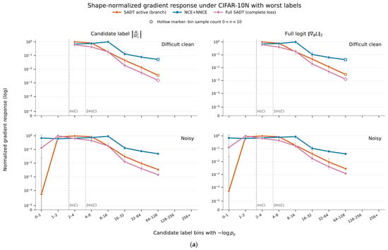
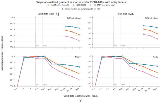
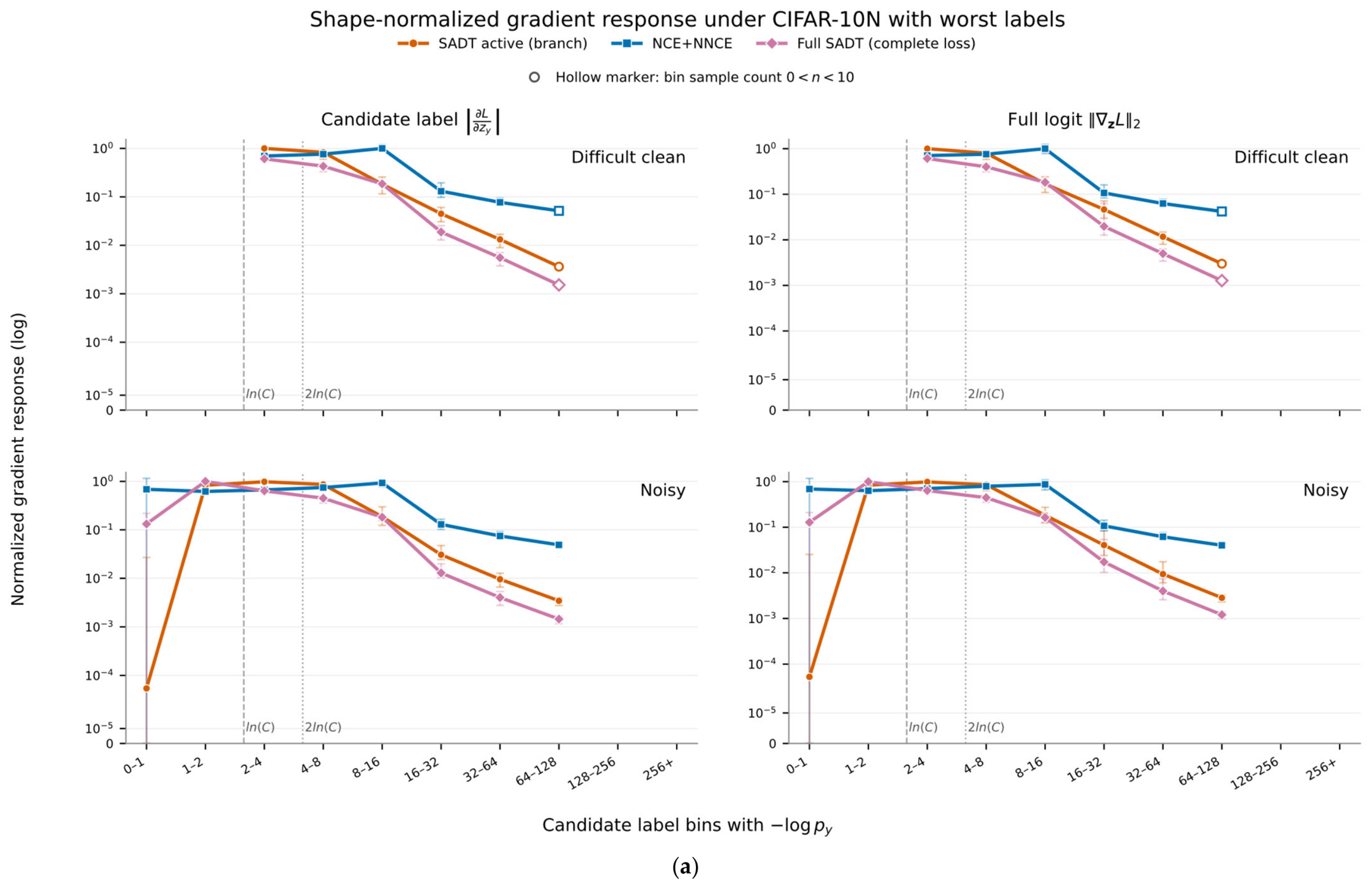
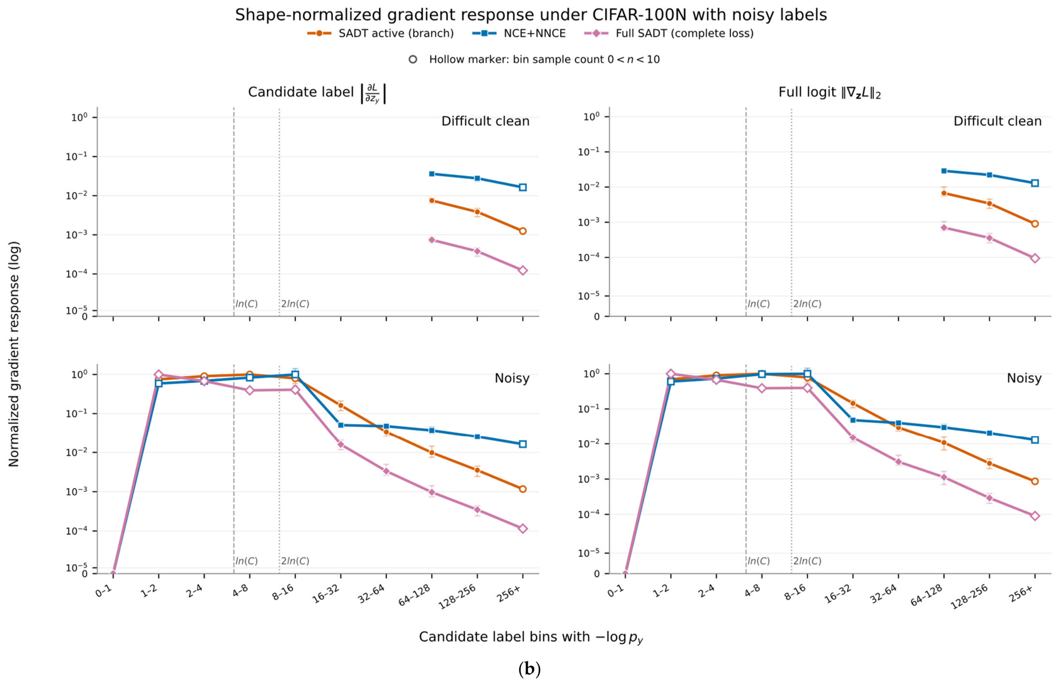
To analyze the gradient regulation mechanism of SADT, we compare its gradient responses with those of NCE + NNCE across different predictive surprise tk = −lnpk intervals using model checkpoints from the same training epoch. As shown in Figure 2, on CIFAR-10N, SADT exhibits more pronounced attenuation of both candidate-label gradients and full-logit gradient norms for high-surprise noisy samples, whereas NCE + NNCE maintains relatively larger gradient responses in the same regions. This indicates that SADT effectively reduces the influence of extremely unlikely labels on model optimization through its dual-tail transformation while retaining informative learning signals in moderate-surprise regions. However, similar gradient attenuation also occurs for some difficult clean samples, particularly on CIFAR-100N, suggesting that stronger tail suppression may weaken learning signals from hard samples. Overall, these results demonstrate that SADT regulates gradient responses according to predictive surprise while revealing a potential tradeoff between noise suppression and effective learning from difficult samples.
Figure 2.
Normalized gradient responses of SADT and NCE + NNCE across predictive surprise intervals on (a) CIFAR-10N with Worst labels and (b) CIFAR-100N with Noisy labels.
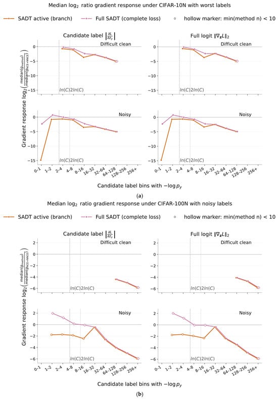
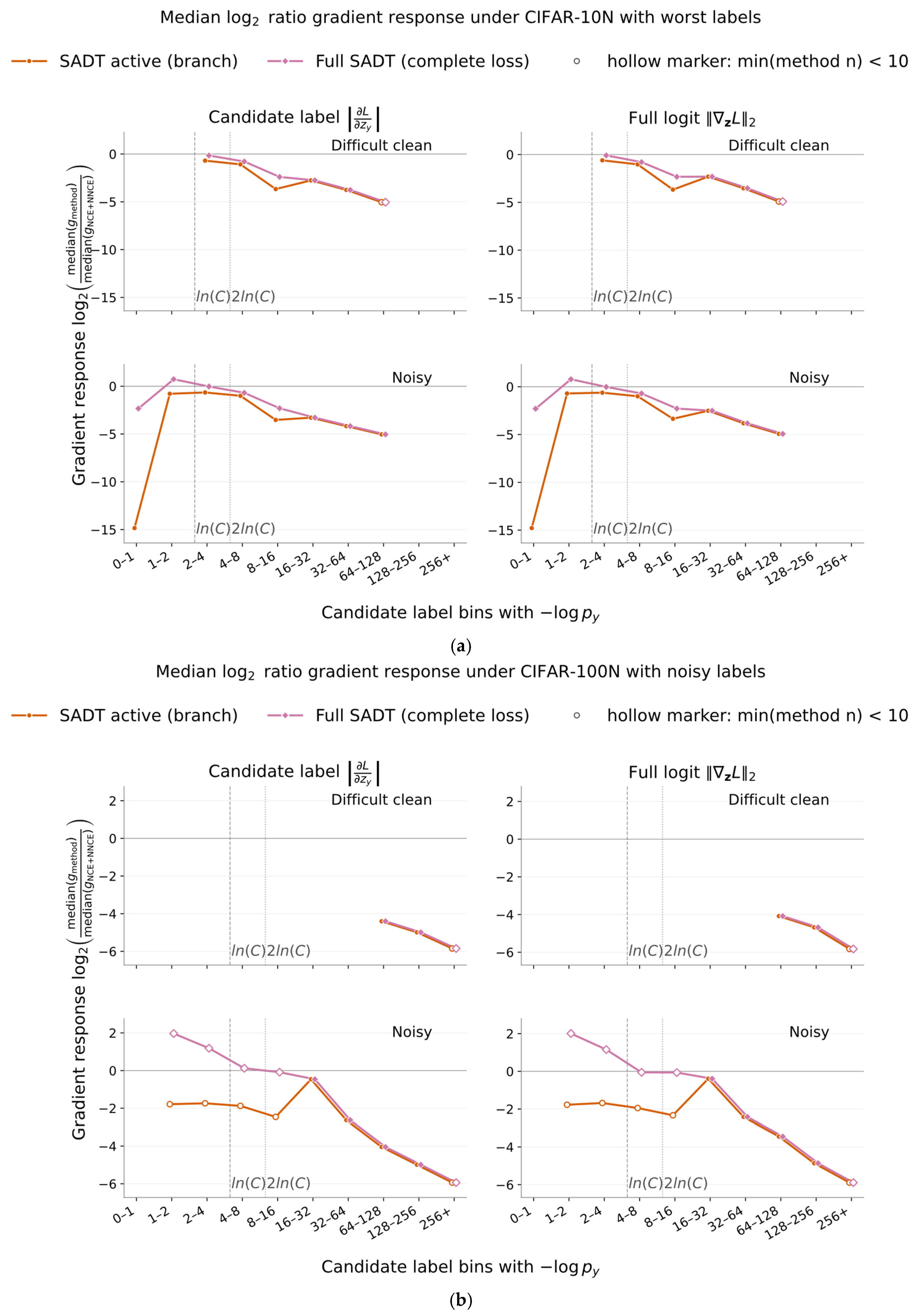
To further quantify the gradient regulation of SADT, Figure 3 presents the log2 ratios of median gradients between SADT and NCE + NNCE across predictive surprise intervals, where negative values indicate smaller gradients for SADT. As shown in Figure 3a, SADT exhibits stronger gradient attenuation in high surprise regions on CIFAR-10N, particularly for noisy samples. A similar trend appears on CIFAR-100N, although substantial attenuation also occurs for some difficult clean samples. These observations are consistent with the performance differences across noise settings. As shown in Table 1, Table 2 and Table 3, SADT achieves notable improvements under several severe noise conditions, including gains of 2.64% and 2.25% over NCE + NNCE on CIFAR-10 with 80% symmetric noise and 40% asymmetric noise, respectively. However, its advantages are less consistent on CIFAR-100, particularly under real human annotation noise. This may be attributed to the stronger gradient suppression of difficult clean samples, which can weaken informative learning signals as classification difficulty increases. Overall, these results highlight the tradeoff between suppressing noisy supervision and preserving effective learning from difficult clean samples, indicating that the robustness of SADT depends on both noise characteristics and classification difficulty.
Figure 3.
Relative gradient responses of SADT and NCE + NNCE across predictive surprise intervals on (a) CIFAR-10N with Worst labels and (b) CIFAR-100N with Noisy labels. The vertical axis represents the log2 ratio of gradient medians relative to NCE + NNCE, where negative values indicate stronger gradient attenuation by SADT.
4.6. Ablation Analysis
Table 6 evaluates the contributions of surprise annealing and the passive component under different noise settings. Removing the passive component substantially reduces accuracy on CIFAR-100, indicating its importance in more challenging classification tasks. However, it improves performance under 40% asymmetric noise on CIFAR-10. Similarly, removing surprise annealing slightly improves several CIFAR-10 results, whereas the full SADT generally performs better on CIFAR-100. These differences suggest that the benefits of the two components depend on noise characteristics and classification difficulty. Stronger suppression of low-confidence predictions may help reduce noisy supervision but can also weaken informative gradients from difficult clean samples. Therefore, the complete SADT aims to balance robustness and effective learning across different settings rather than maximize accuracy under every individual noise condition.
Table 6.
Ablation study under various noisy settings. “x/x” indicates the last/best accuracies.
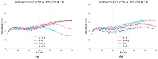
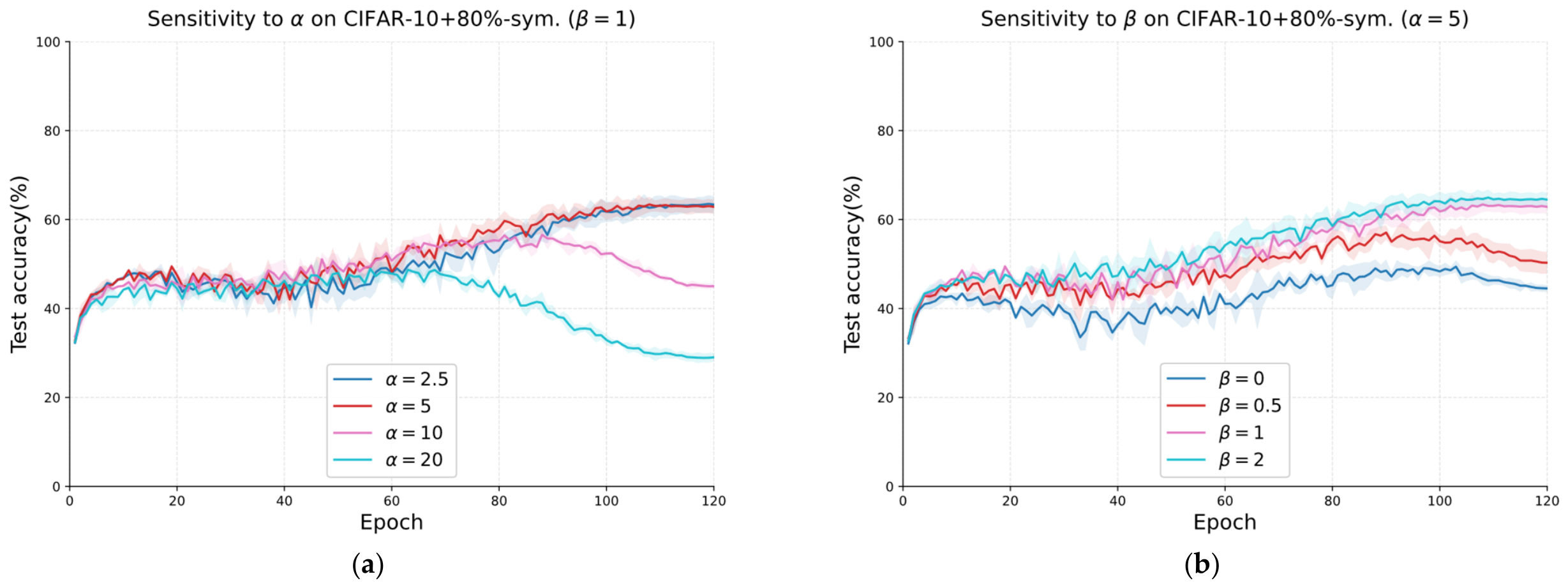
Hyperparameter analysis. We analyze the sensitivity of SADT to α and β on CIFAR-10 with 80% symmetric noise. We vary α ∈ {2.5, 5, 10, 20} while fixing β = 1, and vary β ∈ {0, 0.5, 1, 2} while fixing α = 5. All other training settings remain unchanged. Each configuration is evaluated using three seeds. As shown in Figure 4, the solid curves report the per-epoch mean accuracy, while the shaded regions denote sample standard deviation. Clearly, CIFAR-10 performs consistently well for α ∈ [2.5, 5] and β ∈ [1, 2], whereas excessively large α or small β causes pronounced late-stage degradation. Overall, the adopted settings (5, 1) lie in favorable regions and provide a reliable balance between accuracy and stability without extensive tuning.
Figure 4.
Parameter sensitivity analysis of SADT on CIFAR-10 under 80% symmetric noise. (a) Sensitivity to α with β = 1. (b) Sensitivity to β with α = 5. Solid curves represent the mean test accuracy over three random seeds, and shaded regions indicate sample standard deviations.
Computational cost. SADT requires O(BC) time and temporary memory complexity without additional networks or forward passes. Table 7 compares its practical training cost with CE and NCE + NNCE on Tiny ImageNet under identical conditions. SADT requires 80.84 s per epoch, compared with 80.79 and 80.78 s for CE and NCE + NNCE, respectively. All three methods exhibit approximately 7.13 GB of peak GPU memory consumption. These results indicate that SADT introduces negligible additional training overhead while maintaining comparable memory requirements.
Table 7.
Training cost comparison under Tiny-ImageNet with 40%-Asym.
4.7. Comparison with Existing Robust Loss Functions
Table 8 summarizes the main mechanisms, advantages, and limitations of representative robust loss functions. Existing methods primarily improve noise robustness through generalized loss design, normalization, asymmetric objectives, or gradient regulation. In contrast, SADT combines dual-tail transformation and surprise-dependent annealing to regulate loss responses across different confidence regions while maintaining an exact constant class sum through its active and passive components. However, this design involves additional loss computation operations and may weaken informative gradients from difficult clean samples, particularly in challenging classification tasks. These observations indicate that SADT provides a different approach to balancing noise suppression and effective learning, although its advantages are not consistent across all noise settings.
Table 8.
Comparison of representative robust loss functions.
Overall, SADT offers several benefits, including confidence-dependent loss regulation, an exact constant class sum, and straightforward integration into standard training pipelines without additional networks. Its dual-tail transformation and surprise-dependent annealing provide a flexible balance between noise suppression and effective learning, particularly under severe label noise. Nevertheless, strong suppression of high surprise samples may also weaken informative gradients from difficult clean samples, potentially limiting performance in tasks with more classes. Moreover, SADT requires additional loss computation operations compared with simpler objectives. These limitations suggest that further improvements should focus on balancing sample difficulty and noise suppression more effectively.
4.8. Integration with Existing LNL Methods
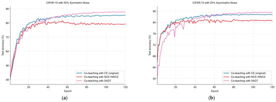
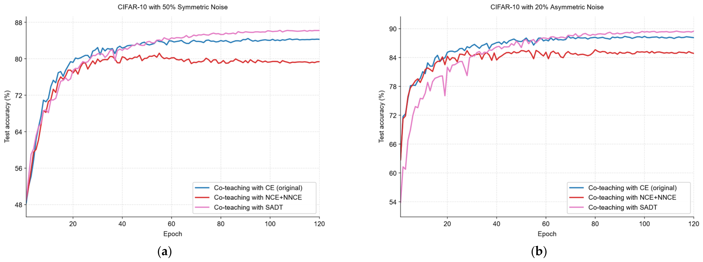
To evaluate SADT’s compatibility with existing noisy-label learning frameworks, we integrated it into Co-teaching [40], replacing CE with SADT or NCE + NNCE for sample loss evaluation while keeping all other settings unchanged. Figure 5 shows the accuracy curves on CIFAR-10 under symmetric and asymmetric noise. These results demonstrate that SADT is compatible with Co-teaching and consistently outperforms NCE + NNCE and CE in the evaluated settings.
Figure 5.
Test accuracy curves of Co-teaching with CE, NCE + NNCE, and SADT under different noise settings on CIFAR-10. (a) 50% symmetric noise. (b) 20% asymmetric noise.
5. Conclusions
In this work, we propose surprise-annealed dual-tail loss for NLL tasks. SADT constructs a continuous dual-tail transformation from predictive surprise, progressively suppressing extremely unlikely labels through inverse hyperbolic sine and arctangent branches while retaining informative learning signals through surprise-dependent annealing. By combining a normalized active score with a log-balanced passive score, SADT achieves an exact constant class sum. Theoretically, we established its boundedness and proved exact preservation of clean risk minimizers under constant uniform symmetric noise. For asymmetric and instance-dependent noise, we further derived posterior ordering-sufficient conditions and a total variation risk bound. Experimental results demonstrate competitive performance across various synthetic and real-world noisy settings, with notable improvements under severe noise conditions. However, gradient analysis also revealed that strong tail suppression may weaken learning signals from difficult clean samples, limiting performance on tasks with larger class counts. Future work will focus on adaptive loss regulation that jointly considers sample reliability and learning difficulty to further improve generalization under complex label noise.
Author Contributions
Q.Z.: Methodology, Software, Resources, Writing—original draft preparation, Visualization, Supervision, Project administration, Funding acquisition; Y.C.: software, Validation; Y.Y.: Validation; G.J.: Investigation, Supervision. All authors have read and agreed to the published version of the manuscript.
Funding
This study is funded by the Qing Lan Project of Jiangsu Province; the National Natural Science Foundation of China, grant number 62206114.
Data Availability Statement
The datasets such as CIFAR-10/100, CIFAR-10/100N, Clothing1M and WebVision employed in this paper are available at http://www.cs.toronto.edu/~kriz/cifar.html (accessed on 1 September 2026), https://github.com/UCSC-REAL/cifar-10-100n (accessed on 1 September 2026), https://github.com/Cysu/noisy_label (accessed on 1 September 2026), and https://data.vision.ee.ethz.ch/cvl/webvision/download.html (accessed on 1 September 2026). Our code is available at https://github.com/LanXiaoPang613/SADT (accessed on 1 September 2026).
Acknowledgments
The authors acknowledge the use of ChatGPT 5.6 instant (OpenAI) for improving the readability and language of the manuscript. The authors reviewed and edited all AI-assisted outputs and take full responsibility for the content of the manuscript.
Conflicts of Interest
The authors declare no conflicts of interest.
References
- Chen, Z.; Fan, Q.; Jiao, R.; Xue, B.; Huang, H.; Dai, Y.; Zhang, M. Multi-expert genetic programming based ensemble for long-tailed image classification. IEEE Trans. Evol. Comput. 2026. [Google Scholar] [CrossRef] [Scilit]
- Müller, P.; Braun, A.; Keuper, M. Examining the impact of optical aberrations to image classification and object detection models. IEEE Trans. Pattern Anal. Mach. Intell. 2025, 48, 2139–2153. [Google Scholar] [CrossRef] [Scilit] [PubMed]
- Zhang, Y.; Pang, J.; Zhu, Z.; Liu, Y. Evaluating LLM-contaminated crowdsourcing data without ground truth. Adv. Neural Inf. Process. Syst. (NeurIPS) 2025, 38, 68113–68151. [Google Scholar]
- Kiryu, K.; Miyamoto, M.; Nakamura, A. A Method of Constructing a Food Classification Image Dataset by Cleansing Web-Crawling Data. Int. J. Autom. Technol. 2025, 19, 608–617. [Google Scholar] [CrossRef] [Scilit]
- Ghosh, A.; Kumar, H.; Sastry, P.S. Robust loss functions under label noise for deep neural networks. Proc. AAAI Conf. Artif. Intell. 2017, 31, 1919–1925. [Google Scholar] [CrossRef] [Scilit]
- Zhang, Q.; Chen, Q. UCRT: A two-stage noisy label learning framework with uniform consistency selection and robust training. Appl. Intell. 2026, 56, 21. [Google Scholar] [CrossRef] [Scilit]
- Ghosh, A.; Manwani, N.; Sastry, P.S. Making risk minimization tolerant to label noise. Neurocomputing 2015, 160, 93–107. [Google Scholar] [CrossRef] [Scilit]
- Liang, J.; Li, Y.; Cui, J. Label Noise Correction via Fuzzy Learning Machine. Proc. AAAI Conf. Artif. Intell. 2025, 39, 18676–18683. [Google Scholar] [CrossRef] [Scilit]
- Shi, C.; Lu, L.; Zhao, M.; Hei, X.; Pun, C.-M.; Miao, Q. Learning hyperspectral noisy label with global and local hypergraph laplacian energy. Pattern Recognit. 2025, 165, 111606. [Google Scholar] [CrossRef] [Scilit]
- Fan, W.; Li, K. Combating Semantic Contamination in Learning with Label Noise. Proc. AAAI Conf. Artif. Intell. 2025, 39, 2870–2878. [Google Scholar] [CrossRef] [Scilit]
- Hou, S.; Xu, M.; Jiang, G.; Guo, Y.; Wang, W. Outlier-trimmed dual-interval smoothing loss for sample selection in learning with noisy labels. Neural Netw. 2025, 191, 107827. [Google Scholar] [CrossRef] [Scilit] [PubMed]
- Pan, W.; Wei, W.; Xie, W. Debiased Sample Selection for Learning with Noisy Labels. In Proceedings of the IEEE/CVF Conference on Computer Vision and Pattern Recognition (CVPR), Denver, CO, USA, 3–7 June 2026; pp. 32047–32057. [Google Scholar]
- Zhao, Y.; Xia, Q.; Sun, Y.; Wen, Z.; Ma, L.; Ying, S. Open set label noise learning with robust sample selection and margin-guided module. Knowl.-Based Syst. 2025, 321, 113670. [Google Scholar] [CrossRef] [Scilit]
- Zhou, X.; Liu, X.; Jiang, J.; Gao, X.; Ji, X. Asymmetric loss functions for learning with noisy labels. Proc. Int. Conf. Mach. Learn. 2021, 139, 12846–12856. [Google Scholar]
- Zhou, X.; Liu, X.; Zhai, D.; Jiang, J.; Ji, X. Asymmetric loss functions for noise-tolerant learning: Theory and applications. IEEE Trans. Pattern Anal. Mach. Intell. 2023, 45, 8094–8109. [Google Scholar] [CrossRef] [Scilit] [PubMed]
- Ye, X.; Li, X.; Dai, S.; Liu, T.; Sun, Y.; Tong, W. Active negative loss functions for learning with noisy labels. Adv. Neural Inf. Process. Syst. (NeurIPS) 2023, 36, 6917–6940. [Google Scholar] [CrossRef] [Scilit]
- Zhang, Z.; Sabuncu, M.R. Generalized cross entropy loss for training deep neural networks with noisy labels. Adv. Neural Inf. Process. Syst. (NeurIPS) 2018, 31, 8792–8802. [Google Scholar]
- Wang, Y.; Ma, X.; Chen, Z.; Luo, Y.; Yi, J.; Bailey, J. Symmetric cross entropy for robust learning with noisy labels. In Proceedings of the IEEE/CVF International Conference on Computer Vision, Seoul, Republic of Korea, 27 October–2 November 2019; pp. 322–330. [Google Scholar]
- Ma, X.; Huang, H.; Wang, Y.; Romano, S.; Erfani, S.; Bailey, J. Normalized loss functions for deep learning with noisy labels. Proc. Int. Conf. Mach. Learn. (ICML) 2020, 119, 6543–6553. [Google Scholar]
- Liu, Y.; Guo, H. Peer loss functions: Learning from noisy labels without knowing noise rates. Proc. Int. Conf. Mach. Learn. 2020, 119, 6226–6236. [Google Scholar]
- Wei, H.; Zhuang, H.; Xie, R.; Feng, L.; Niu, G.; An, B.; Li, Y. Mitigating memorization of noisy labels by clipping the model prediction. Proc. Int. Conf. Mach. Learn. 2023, 202, 36868–36886. [Google Scholar]
- Wang, J.; Liu, X.; Zhou, X.; Hu, G.; Zhai, D.; Jiang, J.; Ji, X. Joint Asymmetric Loss for Learning with Noisy Labels. In Proceedings of the IEEE/CVF International Conference on Computer Vision, Honolulu, HI, USA, 19–23 October 2025; pp. 1947–1956. [Google Scholar]
- Ye, X.; Wu, Y.; Zhang, W.; Li, X.; Chen, Y.; Jin, C. Optimized Gradient Clipping for Noisy Label Learning. Proc. AAAI Conf. Artif. Intell. 2025, 39, 9463–9471. [Google Scholar] [CrossRef] [Scilit]
- Wang, J.; Zhou, X.; Liu, X.; Hu, G.; Zhai, D.; Jiang, J.; Li, H. Variation-Bounded Loss for Noise-Tolerant Learning. Proc. AAAI Conf. Artif. Intell. 2026, 40, 26251–26259. [Google Scholar] [CrossRef] [Scilit]
- Li, J.; Socher, R.; Hoi, S.C.H. DivideMix: Learning with noisy labels as semi-supervised learning. In Proceedings of the International Conference on Learning Representations, Online, 26–30 April 2020. [Google Scholar]
- Li, F.; Li, K.; Tian, J.; Zhou, J. Regroup median loss for combating label noise. Proc. AAAI Conf. Artif. Intell. 2024, 38, 13474–13482. [Google Scholar] [CrossRef] [Scilit]
- Pan, W.; Wei, W.; Zhu, F.; Deng, Y. Enhanced Sample Selection with Confidence Tracking: Identifying Correctly Labeled Yet Hard-to-Learn Samples in Noisy Data. Proc. AAAI Conf. Artif. Intell. 2025, 39, 19795–19803. [Google Scholar] [CrossRef] [Scilit]
- Xu, Y.; Niu, X.; Yang, J.; Su, R.; Zhang, J.; Liu, S.; Drew, S. Revisiting Interpolation for Noisy Label Correction. Proc. AAAI Conf. Artif. Intell. 2025, 39, 21833–21841. [Google Scholar] [CrossRef] [Scilit]
- Sheng, M.; Sun, Z.; Zhou, T.; Shu, X.; Pan, J.; Yao, Y. CA2C: A Prior-Knowledge-Free Approach for Robust Label Noise Learning via Asymmetric Co-learning and Co-training. In Proceedings of the IEEE/CVF International Conference on Computer Vision, Honolulu, HI, USA, 19–23 October 2025; pp. 901–911. [Google Scholar]
- Zhang, W.; Cheng, D.; Lu, G.; Zhou, B.; Li, J.; Zhang, S. Efficient Adaptive Label Refinement for label noise learning. Neurocomputing 2025, 639, 130305. [Google Scholar] [CrossRef] [Scilit]
- Zhang, H.; Cisse, M.; Dauphin, Y.N.; Lopez-Paz, D. mixup: Beyond empirical risk minimization. In Proceedings of the International Conference on Learning Representations, Vancouver, BC, Canada, 30 April–3 May 2018. [Google Scholar]
- Zhang, Q.; Lee, F.; Wang, Y.; Miao, R.; Chen, L.; Chen, Q. An improved noise loss correction algorithm for learning from noisy labels. J. Vis. Commun. Image Represent. 2020, 72, 102930. [Google Scholar] [CrossRef] [Scilit]
- Krizhevsky, A. Learning Multiple Layers of Features from Tiny Images. 2009. Available online: https://cave.cs.toronto.edu/kriz/learning-features-2009-TR.pdf (accessed on 1 September 2026).
- Xia, X.; Liu, T.; Han, B.; Wang, N.; Gong, M.; Liu, H.; Niu, G.; Tao, D.; Sugiyama, M. Part-dependent label noise: Towards instance-dependent label noise. Adv. Neural Inf. Process. Syst. (NeurIPS) 2020, 33, 7597–7610. [Google Scholar]
- Wu, J.; Zhang, Q.; Xu, G. Tiny ImageNet Challenge; Technical Report; Stanford University: Stanford, CA, USA, 2017. [Google Scholar]
- Wei, J.; Zhu, Z.; Cheng, H.; Liu, T.; Niu, G.; Liu, Y. Learning with noisy labels revisited: A study using real-world human annotations. In Proceedings of the International Conference on Learning Representations (ICLR), Online, 25–29 April 2022. [Google Scholar]
- Xiao, T.; Xia, T.; Yang, Y.; Huang, C.; Wang, X. Learning from massive noisy labeled data for image classification. In Proceedings of the IEEE Conference on Computer Vision and Pattern Recognition (CVPR), Boston, MA, USA, 7–12 June 2015; pp. 2691–2699. [Google Scholar]
- Li, W.; Wang, L.; Li, W.; Agustsson, E.; Van Gool, L. Webvision database: Visual learning and understanding from web data. arXiv 2017, arXiv:1708.02862. [Google Scholar]
- He, K.; Zhang, X.; Ren, S.; Sun, J. Deep residual learning for image recognition. In Proceedings of the IEEE/CVF Conference on Computer Vision and Pattern Recognition (CVPR), Las Vegas, NV, USA, 27–30 June 2016; pp. 770–778. [Google Scholar] [CrossRef] [Scilit]
- Han, B.; Yao, Q.; Yu, X.; Niu, G.; Xu, M.; Hu, W.; Tsang, I.; Sugiyama, M. Co-teaching: Robust training of deep neural networks with extremely noisy labels. Adv. Neural Inf. Process. Syst. (NeurIPS) 2018, 31, 8536–8546. [Google Scholar]

Disclaimer/Publisher’s Note: The statements, opinions and data contained in all publications are solely those of the individual author(s) and contributor(s) and not of MDPI and/or the editor(s). MDPI and/or the editor(s) disclaim responsibility for any injury to people or property resulting from any ideas, methods, instructions or products referred to in the content. |
© 2026 by the authors. Licensee MDPI, Basel, Switzerland. This article is an open access article distributed under the terms and conditions of the Creative Commons Attribution (CC BY) license.