


Abstract
We study the entanglement between an electron and the photon it scatters, resolved in real space and time. Starting from nonrelativistic QED in Fermi’s oscillator representation, we write Fock’s coupled equations for the components with a fixed photon number in the configuration space of the photons, in the length gauge, where the photon is created around the atom with a nonlocal kernel. Truncated at one photon, the equations are solved numerically, without the rotating-wave approximation, for a one-dimensional model atom in a waveguide with a single transverse mode and an enhanced coupling, driven by a short off-resonant laser pulse, with the electron and the photon on real-space grids. The global electron–photon entanglement is largely transient. It peaks during the pulse and decreases when the polarized electron cloud returns to the core, leaving a state close to a product of the electron state and a superposition of the field vacuum with one scattered photon. Local entanglement, obtained from walkers sampled over both photon-number components, shows opposite patterns for the two particles. The electron entropy is smallest at the nucleus and maps the local strength of the dipole coupling, while the photon entropy is largest near the atom, where photons are created and absorbed, and smaller in the outgoing packets.
1. Introduction
The interaction of light with matter is usually described on one of two levels. In the semiclassical picture, the electrons are quantum particles, while the field obeys Maxwell’s equations with the mean electron current as its source. In quantum electrodynamics (QED) the field is quantized as well [1,2,3]. With self-consistent backreaction, the semiclassical picture accounts for absorption, stimulated emission, and coherent scattering, but it fails for processes in which the number of photons matters. An atom prepared in a pure excited state never decays because its mean dipole vanishes, a single photon does not give coincident counts at two separated detectors [4], and resonance fluorescence shows no antibunching [5]. In all these processes, the state of the electrons and the state of the field are entangled, and it is this electron–photon entanglement that we want to follow in real space and time.
The standard route to QED expands the transverse field in modes, each a harmonic oscillator. Numerical methods for atoms and molecules in cavities follow this route, either exactly in a truncated photon-number space or approximately, as in QED Hartree–Fock and coupled-cluster theory [6] and in diffusion Monte Carlo with the mode coordinate as an additional walker coordinate [7]. In these methods, the position of a photon is not a variable, and the cost grows with the number of modes rather than with the number of photons. Entanglement in real space requires a description in which the photon has a coordinate of its own.
Such a description goes back to Landau and Peierls [8], who wrote QED as a Schrödinger equation for a sequence of wave functions with photons in configuration space. Fock showed that these sequences are equivalent to second quantization [9] and formulated QED as coupled equations for the components with a fixed photon number [10]. When truncated at one photon, they give the Breit interaction and the natural linewidth. The real-space photon amplitude with a local probability density is the number, or Landau–Peierls, amplitude [11,12,13,14]. It differs from the energy amplitude, the positive-frequency Riemann–Silberstein field normalized to one quantum, by the nonlocal factor , which reflects the absence of localized photon states and enters the coupling of the photon to the charges.
Real-space photons coupled to emitters are standard in waveguide QED [15,16], mostly for two- or three-level emitters within the rotating-wave approximation (RWA). Atom–photon entanglement in real space has been obtained from the Wigner–Weisskopf amplitudes of two-level atoms with recoil [17,18], and numerical solutions exist for two-level atoms coupled to many cavity modes in the space of a single excitation [19,20]. The single-mode form of Fock’s equations, with the driving laser as the quantized mode and in the velocity gauge, has been solved for strong-field ionization [21], where the entanglement arises from the spread in the number of photons absorbed from the drive, which contains up to photons, and spontaneous emission is neglected as a correction of order . In the quantum optics of strong-field processes the coherent drive is split into a classical field and its quantum fluctuations, and all modes start from the vacuum. When the field couples only to the mean dipole, it ends in a product of coherent states, and nonclassical and entangled states of light are obtained by conditioning on high-harmonic generation or above-threshold ionization [22]. These treatments use field modes and do not resolve the photon in space. To our knowledge, the photon-number equations have not been solved for an electron on a real-space grid, including its continuum, with the photon in position space and without the RWA.
In this work, we use waves and walkers in a quantum Monte Carlo approach [23,24,25], but the conditional waves are slices of the exact numerical solution of the Schrödinger equation at the positions of the walkers. In the configuration-space form of QED, a walker carries an electron coordinate and, in the one-photon component, also a photon coordinate. Grouping the walkers by their positions, we define the entanglement locally, since the reduced density matrix of a spatial region is built from the conditional waves of the walkers located in it [26].
We first write Fock’s photon-number hierarchy in the configuration space of the photons, in the length gauge, starting from Fermi’s oscillator representation of the field; the photon is created around the atom with the kernel , and the truncation at one photon fixes how the polarization energy enters each component. Second, we solve the truncated equations without the RWA for an electron on a real-space grid coupled to a continuum of guide modes. Third, we apply the strip construction of local entanglement to both particles, with the walkers distributed in the configuration space of the electron–photon system. Section 2 contains the derivation and the waveguide model, and Section 3 the numerical method and the results for an atom driven by a short off-resonant laser pulse.
2. Nonrelativistic QED in the Configuration Space of Photons
2.1. Electrons and the Transverse Field
We consider electrons of charge and mass at the positions , bound to a nucleus of charge held fixed at . We split the electric field into its longitudinal and transverse parts, , with and . Gauss’s law, , fixes at every instant by the positions of the charges, and its energy is the Coulomb energy. After the infinite self-energies of the point charges are dropped, this energy becomes the potential
In the Coulomb gauge, , the vector potential is purely transverse, and . The Hamiltonian of the electrons and the field is [27]
where is the canonical momentum of electron . The minimal coupling in the first term gives the Lorentz force on the electrons and, through the same action, the transverse current as the source of the field. The photons are the quanta of the transverse dynamical field.
2.2. Dipole Approximation and the Length Gauge
We place the field in a periodic box of volume and expand it in a complete set of real, orthonormal, transverse mode functions , with , and . In free space, these are standing waves and times two polarization vectors perpendicular to . Their completeness relation defines the transverse delta function, with the Cartesian components labelled by the Greek indices ,
With the real amplitudes we write
Inserting these into the field energy, and using , we obtain a sum of oscillators of unit mass with the frequencies ,
where is the momentum conjugate to . This is Fermi’s form of the radiation field [3]. We quantize it in the Schrödinger representation, with one wave function of all electron coordinates and all field amplitudes, and . The free field Hamiltonian is
The constant , the zero-point energy of the field oscillators, is subtracted, and all energies are counted from the field vacuum, the state in which every oscillator is in its ground state. The eigenfunctions of each oscillator are the normalized Hermite functions with the energies above the vacuum, and is the number of photons in mode .
We write for the electron coordinates relative to the nucleus, and for the dipole of the neutral atom (). The electrons are bound within a few Bohr radii, while the wavelengths that couple to them are much longer. In the dipole approximation we replace by . For an atom of size the neglected electric-quadrupole and magnetic-dipole couplings are of relative order for the coupled wave numbers . The Hamiltonian becomes
Since is a linear function of the field amplitudes, the transformation to the length gauge [28] is in Fermi’s representation simply the multiplication of the wave function by a phase that depends on the electron and field coordinates:
The phase shifts the electron momenta by , which removes the vector potential from the kinetic energy, and it shifts each field momentum by . Expanding the field energy with the shifted momenta, we arrive at the length-gauge Hamiltonian
with
The field that couples to the dipole is the transverse displacement field , with the polarization ; outside the atom it coincides with the electric field [27,29]. The term quadratic in has disappeared, and in its place appears the transverse polarization energy , often called the dipole self-energy [30]. It is not added to the Hamiltonian. Writing the radiation energy of Equation (2) with gives
and is the part of the transverse field energy carried by the polarization of the atom. Together with the coupling it completes a square in each field oscillator, , which makes bounded from below; without it the length-gauge Hamiltonian has no ground state [30].
2.3. Components with Fixed Photon Number
The coupling in Equation (9) is linear in the field momenta. In the Schrödinger representation of the field, the momentum acts on the Hermite functions as
which follows from the recursion relations of the Hermite polynomials. Each action of the coupling therefore changes the number of photons by one. We expand in products of oscillator eigenfunctions and collect the terms with the total photon number . Following Fock [9] we write the coefficients of these terms as functions that are symmetric in the mode labels and antisymmetric in the electron coordinates; a product state with photons in mode enters with the coefficient . With this convention the normalization takes the form
and is the probability density of finding the electrons at together with photons in the modes . We introduce the field of one photon in mode at the nucleus,
which gives . Inserting the expansion into , using Equation (12) and projecting onto the oscillator states, we obtain the hierarchy
where means that the label is left out. The second term on the right is the absorption of one photon from the component with photons, the third term the emission of one photon from the component with photons. Equation (15) has the structure of Fock’s coupled equations, here in the length gauge. Creation and annihilation operators are not needed for it, as they are only a shorthand for Equation (12). The oscillator amplitudes appear only in the derivation and are absent from the result.
2.4. Photons in Real Space
For each photon we transform the mode label into a position and a Cartesian index ,
Since the form an orthonormal basis of the transverse fields, Equation (16) is a unitary map onto transverse functions of each photon coordinate, and the normalization (13) becomes the integral of over all electron and photon coordinates. The components are the number amplitudes of the photons, and is the joint probability density of the electrons and of photons in configuration space. The photon energy becomes the operator , where multiplies each plane wave by . The coupling constants combine into the kernel
which is real, even and transverse. is the field at the nucleus that belongs to one photon at ; read in the other direction, it is the shape with which a photon is created around the nucleus. Away from the origin has the form of a static dipole field, , and the factor steepens it to a tail . The emitted photon is born with a power-law tail around the atom, not at a point; this is where the photon localization problem enters the dynamics. Transforming Equation (15) photon by photon we obtain the hierarchy in real space:
In the absorption term the vector index of the absorbed photon is contracted with , in the emission term the new photon carries the index of . Up to the dipole approximation, Equation (18) is the Schrödinger equation of nonrelativistic QED in the configuration space of electrons and a variable number of transverse photons. Several of its features are needed below.
- (i)
- The vacuum. The bare field vacuum is the component without photons; it carries no photon coordinate and is not represented by photon walkers. Vacuum fluctuations of the free field do not appear because energies are counted from the vacuum. Spontaneous emission and the radiative level shifts are nevertheless contained in Equation (18), in the form in which they are attributed to the reaction of the atom to its own field [31].
- (ii)
- The source. The emission term is driven by the amplitude , by the transition dipole of the electrons, and not by the mean dipole , which vanishes for an eigenstate of the atom. This is the difference from the semiclassical equations with backreaction, in which an atom in an excited eigenstate does not radiate.
- (iii)
- Number and energy amplitudes. The absorption term contains , which is proportional to the energy amplitude of Białynicki-Birula and Sipe [11,12] at the nucleus. The atom absorbs according to the energy amplitude and not according to the number density at its position, in agreement with photodetection theory [32].
- (iv)
- Gauge dependence of the photon number. The transformation (8) displaces the field oscillators by an amount that depends on the electron coordinates. A state without photons in the length gauge contains a cloud of photons in the Coulomb gauge, and the converse holds for the dressed ground state. The photon number of a bound state is therefore not an observable on its own, while the total energy, the electron density and the field measured far from the atom are gauge independent.
- (v)
- What the photon coordinate means. The photon has no position operator with localized eigenstates [14], and the photon state vector is often said to have no position-space representation [20]. Equation (16) does not contradict this, since it is a unitary change in the labels of the one-photon states from modes to points, and is a probability density for the label . It is neither the probability that a point detector at responds nor the energy density of the field there; the energy amplitude is local in the field but is not a probability amplitude. Statements about the position of the photon refer to the number amplitude and are sharp only on scales larger than the wavelengths that make up the photon; for the scattered packets of Section 3 this scale is , against a packet width of
2.5. Truncation at One Photon and the Polarization Energy
We keep the components without and with one photon, and , and set . This is Fock’s truncation of his hierarchy [10], known from its later use in meson theory as the Tamm–Dancoff approximation [33,34]. For the electron-photon interaction, from Equation (18) we obtain two coupled equations for the vacuum component and for the one-photon component :
Without the RWA the number of excitations is not conserved, and what is truncated is the number of photons present at the same time, not the order in the coupling, and the coupled components contain the emission, reabsorption and re-emission of the photon to all orders. A direct projection of onto the two components would keep in both of them. For an atom without a photon, the first-order shift by and the second-order shift by one virtual photon each grow with the cutoff, but by the closure relation over the atomic states their leading growth cancels. In three dimensions the remainder still contains a term quadratic in the cutoff, which by the Thomas–Reiche–Kuhn sum rule is the same for all levels, a linear term, which is removed by mass renormalization, and Bethe’s logarithmic term [35]. In the component with one photon the process that would cancel leads to two photons, which have been removed by the truncation, and would remain there as an uncompensated shift in every atom that has emitted, growing with the cutoff. We therefore adopt a sector-dependent prescription and keep only in the component without a photon, where it is compensated within the retained components. Counterterms that depend on the Fock sector are standard in truncated Fock-space methods [36], and Dancoff [34], like Fock, dropped the self-energy from the truncated equations.
The prescription is an approximation motivated by the processes removed with the truncation, and we test it in Section 3 through the cutoff dependence of the entanglement induced by the pulse. A consequence of the prescription is that at large the potential of the waveguide model (Section 2.6) acts on the component without a photon only.
2.6. One-Dimensional Waveguide Model
From here on we use atomic units, and . The atom is placed in a waveguide with its axis along that carries a single dispersionless transverse mode, uniform over the cross-section at the atom and polarized along . The guide is closed into a ring of length , with the wavenumbers and the frequencies ; the mode carries no field and is left out. One electron moves along the polarization direction with the coordinate , the nucleus is fixed at , and the dipole is . The atomic Hamiltonian is the soft-core model
whose ground-state energy is , with the first excited state at ; the transition frequency is (, ) and the transition dipole . In the guide the photon amplitude reduces to , and we write . With , Equations (19) and (20) become
where multiplies by . The coupling kernel and the constant of the polarization energy are
Here is the field of one photon of mode at the atom. is real and even, with , a positive core at the atom and a negative tail , the one-dimensional counterpart of . The constant grows linearly with the largest wave number in the sum, while in the guide the remainder of the level shift (Section 2.5) grows only logarithmically, because the density of modes is constant in and . No mass counterterm is needed. For the decay of the first excited eigenstate of to its ground state , the golden rule, , gives with Equation (24) and emission in both directions the rate
and we fix the cross-section by choosing . With , , the coupling is much stronger than for an atom in free space. It corresponds rather to an engineered emitter in a strongly confining structure, and it makes the electron–photon correlations large enough to be resolved numerically.
The term couples the electron to the laser pulse, whose classical field is polarized along . Displacing the laser modes by their coherent amplitude [22] leaves the quantized field in its vacuum and adds to in Equations (15)–(20), where is the laser field at the atom. The photon number in the guide therefore counts only the scattered quanta, and a scattered photon of any frequency, including the harmonics of the laser, belongs to the one-photon component. Since the gauge transformation (8) commutes with , the pulse enters both components in the same way.
The emission and absorption terms in Equations (22) and (23) carry the same real kernel with opposite imaginary factors, and the total probability , with the component weights and , is conserved. The photon term is not a differential operator and has no local probability current. On the right-moving () and left-moving () parts of it reduces to , and the photon is transported rigidly at ; the two parts overlap only near the atom.
In the waveguide model the guide field is polarized along and varies only along , while the electron moves along and the nucleus is fixed, so the dipole approximation is exact. For a real atom the corrections are of relative order ; with this is for photons at and at the grid cutoff. The uniform transverse profile requires a guide wider than the atom, while Equation (25) with gives a.u.; we therefore regard as an effective coupling parameter. Recoil of the atom, a separate source of atom–photon entanglement [17], is excluded by the fixed nucleus.
Coupling ratios of this order are reached by superconducting artificial atoms coupled to open transmission lines, which have been taken into the nonperturbative ultrastrong regime [37], and waveguide QED provides the general framework for emitters coupled to one-dimensional continua [38]. Our value, , lies below the onset of the ultrastrong regime, for an emitter coupled to a continuum [37], in analogy with the threshold of cavity QED [39]. We keep the counter-rotating terms mainly for another reason. The laser is detuned from the first line by , which is not small compared with , and the photon cloud of the dressed ground state is created by the counter-rotating terms alone.
2.7. Electron–Photon Entanglement: Global and Local
The state is a pure state of the electron and the photon. The state space of the photon consists of the vacuum and the one-photon states at the positions , and the state of the system is . Its probability density is defined on two sheets of configurations, on the line of configurations without a photon and for configurations with one photon, with the total weight . The trace over the photon gives the reduced density matrix (RDM) of the electron,
and the trace over the electron gives the RDM of the photon, , with a vacuum block, a one-photon block and coherences between them,
Since the state is pure, the two RDMs have the same nonzero eigenvalues . We use the von Neumann entropy . All entropies refer to the partition between the electron and the transverse field of the length gauge, . Since the transformation (8) acts on the electron and the field together, the entropies depend on this choice of partition. Far from the atom coincides with the electric field, and an outgoing photon is described by the same field in both gauges, which does not make the entropies themselves independent of the partition.
When the electron state in the photon component is orthogonal to , for all , as it is in the ground state by parity, the coherences in Equation (27) vanish, and the entropy separates into a photon-number part and a part within the one-photon component,
where the last entropy is that of the normalized one-photon component alone.
For the local entanglement we follow the strip construction of Refs. [25,26]. We introduce an ensemble of M walkers, points in the configuration space of the electron and the photon sampled from the probability density of their joint state, given by the numerical solution. The conditional wave of a walker is the wave function of one particle with the coordinate of the other fixed at that of the walker. A walker without a photon () carries an electron coordinate and is distributed with , and a walker with a photon () carries the pair and is distributed with . The electron wave conditioned on walker is the slice of the state at the photon configuration of the walker,
where is the photon number density, and the photon state conditioned on walker is the slice at its electron coordinate,
which contains the vacuum amplitude next to the one-photon wave. A strip is a range of the coordinate of the particle whose RDM we want. An electron strip contains the walkers with in it, of them without a photon, and its RDM is the average of the projectors on the electron waves (29),
where denotes the walkers of the strip with a photon. A photon strip contains the walkers with in it, the walkers without a photon forming one additional domain, and its RDM is the average of the projectors on the photon states (30),
Its elements , and are the averages over the walkers of the strip of , and , each divided by , and have the structure of the global photon RDM (27). The local von Neumann entropy of a strip is
with or . Each strip RDM is an average of normalized projectors and is therefore positive, with unit trace. It describes the particle conditioned on its position in the strip, as after a weak measurement of the position followed by postselection [26], and its entropy measures the entanglement between the particle localized in the strip and the other particle. For a product state all conditional waves coincide and every strip entropy vanishes; the interaction makes the conditional waves of the walkers in a strip differ from one another, and the strip entropy grows with this diversity. This local entanglement of one particle with the whole of the other is not the entanglement between two regions of space. When all walkers belong to one strip, Equations (31) and (32) reproduce the global RDMs (26) and (27) for a large number of walkers. If the one-photon component is a product, with , all walkers with a photon carry the same electron wave, the RDM of an electron strip has two orthogonal blocks with the weights and , and its von Neumann entropy is the binary entropy ; the local entropy records how the photon number is mixed locally. When the electron state that goes with the photon depends on the photon position, the electron waves in Equation (31) differ from walker to walker, and the strip entropy acquires a spatial structure of its own.
3. Numerical Implementation and Results
Both coordinates are discretized on uniform periodic grids, the electron with points and , the photon with points in the box , which allows propagation up to a.u., and all derivatives are taken spectrally by fast Fourier transform. The photon grid spacing a.u. sets the largest coupled wavenumber, ( a.u., or eV). The atomic eigenstates are obtained by diagonalizing on the electron grid; they provide and the values and , from which Equation (25) with gives the cross-section . The coupling constants of Equation (24) are set on the photon grid, with the Nyquist mode uncoupled to keep real, and follows by one inverse FFT; its norm is .
The time evolution uses symmetric (Strang) splitting of the propagator over the time step . The kinetic energy of the electron and the photon energy are applied as phase factors in Fourier space, half a step before and half a step after the other terms, and the potential , the same in both components, is applied as a phase factor on the grid. The polarization energy acts only on and is applied in two half steps around the coupling step. The coupling terms are the only ones that are neither local on the grid nor diagonal in Fourier space; at each grid point they connect the amplitude with the whole photon wave . Keeping only these terms in Equations (22) and (23), and writing the amplitude of the photon wave along the normalized kernel as , we obtain
while the part of orthogonal to does not change. At each the coupling therefore acts only in the two-dimensional space of the state without a photon and the one-photon state of shape , where Equation (34) describes a rotation of the two amplitudes with the angular velocity . Its exact solution over the step is
where , and and on the right are the values before the step. The step is exact and unitary, conserves to round-off, and costs one projection and one update along per grid point. An absorbing mask over the outer a.u. of the electron grid acts on both components after each step.
The dressed ground state is obtained with the same steps in imaginary time, , where the phase factors become decay factors, the rotation (35) becomes the corresponding hyperbolic transformation, and the total norm is restored after each step. Starting from , , the relaxation converges to the lowest state of Equations (22) and (23) without the pulse, the atom together with the photon component bound to it. The relaxed state is then propagated with the pulse from . The pulse is Gaussian, centred at , with the peak field (peak intensity W/cm2), an intensity FWHM of fs and the carrier frequency ( nm, eV), off-resonant between the lines ( eV) and ( eV) and below the ionization energy of eV.
For the spatial profiles, walkers sample by the Metropolis algorithm. For the strip entropies we sample walkers independently from on the grids of both components, divide them into strips and form the RDMs (31) and (32) with the strict conditional waves (29) and (30), slices of the exact solution at the walker positions. On the grid the photon state (30) is the vector in the orthonormal basis of the vacuum and the grid states . Walkers in the same grid cell carry the same conditional wave, so the sums over the walkers are taken cell by cell with the number of walkers in each cell. The statistical error of the strip entropies decreases as ; at it is about in the central electron strips.
The propagation was checked in two ways. Halving the time step to changes the global entropy by less than at all times. Starting from the bare excited state without a pulse, the atom decays with the rate , against the golden-rule value of Equation (25).
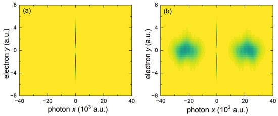
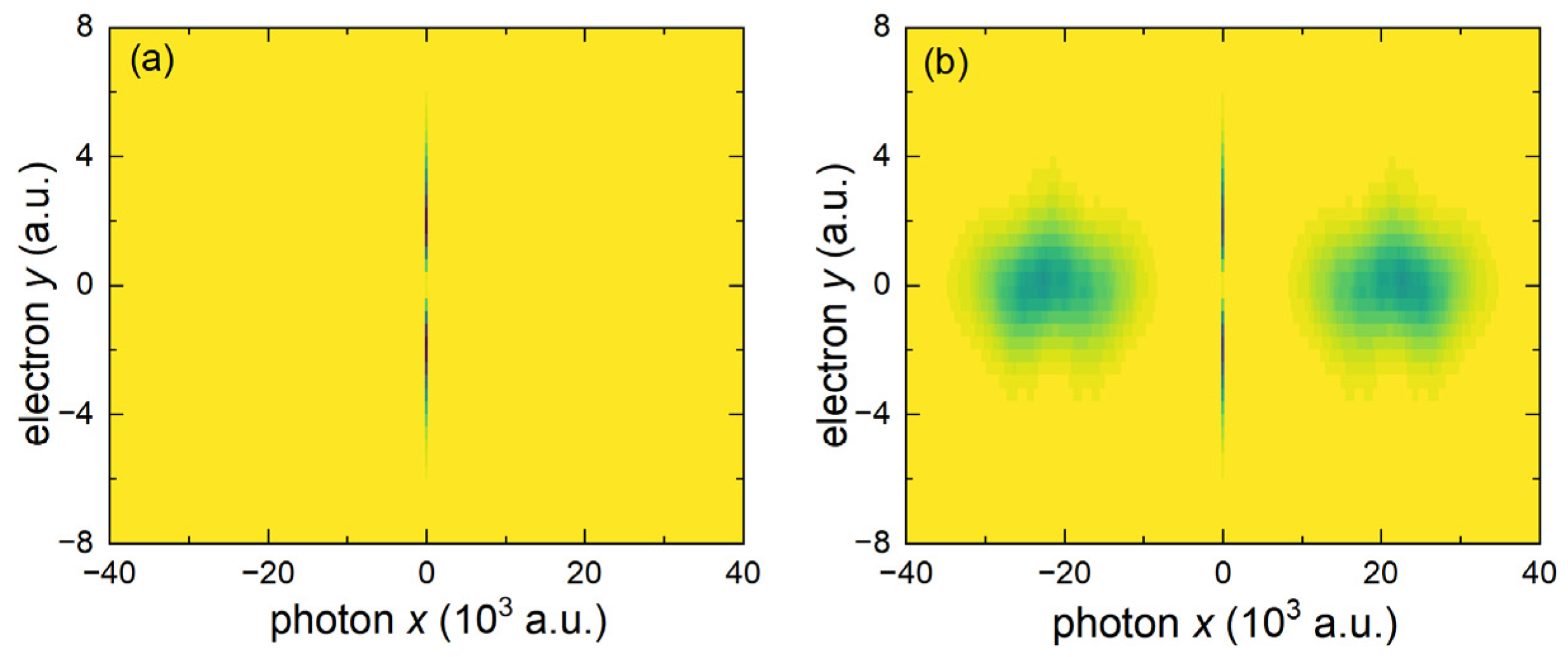
We now apply the method to the atom of Section 2.6 driven by the laser pulse. The propagation stops at the end of the pulse, , and the photon cutoff energy is a.u. ( eV) unless stated otherwise. We report von Neumann entropies throughout. The relaxation in imaginary time gives the dressed ground state with the one-photon weight . The electron state of the one-photon component is odd in , while is even, and the decomposition (28) applies. The photon-number part accounts for nearly the whole global entropy , and the entanglement within the one-photon component adds only . Figure 1a shows the joint probability density of the electron at and the (virtual) photon at . This component is not an emitted photon but the photon cloud of the dressed field vacuum, the part of the dressed ground state in which the electron and the field are correlated, and it carries no energy away. How large it appears depends on the field variable used to count photons (Section 2.4), while the dressed state itself, its energy and the field far from the atom do not. It forms a narrow column at , split into two lobes in with a node at , where the coupling of Equations (22) and (23) vanishes. The truncation at one photon suffices for this dressing, because the counter-rotating part of the coupling connects the atom without a photon directly with the one-photon component.
Figure 1.
Joint probability density of the electron at and the photon at in the one-photon component, on a common linear colour scale from yellow (zero) to dark blue (maximum), (a) at , before the pulse (ground state dressed by the field vacuum), and (b) at the end of the pulse. The weight of the one-photon component is in (a) and in (b). The column at is the vacuum field correlated with the electron; the two lobes in (b) are the two packets of the scattered photon moving along the guide.
Figure 1b shows the joint distribution at the end of the pulse. The scattered photon has separated into two packets that move along the guide with the speed of light in opposite directions. They are centred at , with a full width at half maximum of , of the order of times the duration of the pulse, while the column at the atom has returned close to its ground-state form and carries of . Within each packet the electron is distributed as in the component without a photon, and its distribution does not depend on the position of the photon.
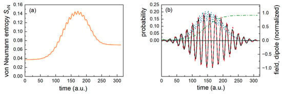
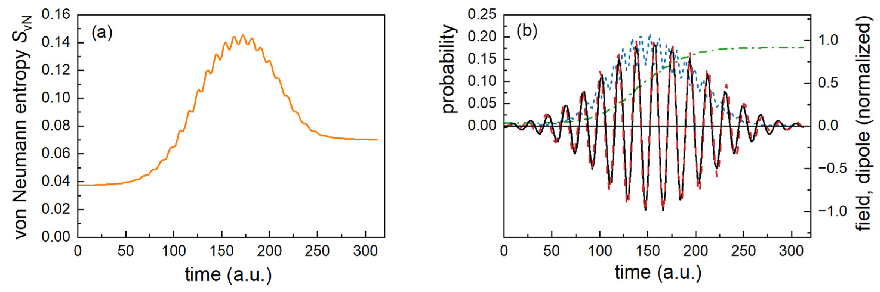
The global von Neumann entropy (Figure 2a) rises from to at , shortly after the maximum of the pulse, and falls to at the end. The change induced by the pulse, , which does not contain the gauge-dependent photon-number part of the dressed ground state, is at the maximum and at the end, although the photon weight stays at , so the entanglement between the electron and the photon is mostly transient. The entropy and the probability of the excited atom (Figure 2b) fall together after the maximum of the pulse, when the part of the electron cloud that the field has driven away from the nucleus returns to the core (recombination). Since the absorber removes less than of the probability, the returning part is the polarized bound cloud rather than ionized electrons, and the atom ends close to its dressed ground state whether a photon was scattered or not. Equation (28) shows why this removes most of the entanglement. If the electron states of the two components were orthogonal, as in the ground state, the photon-number part alone would give at the end. After the return to the core, however, the electron state of the one-photon component nearly coincides with that of the component without a photon. With the prescription of Section 2.5 the change in the entropy induced by the pulse converges for cutoffs two and three times larger, obtained with shorter boxes of the same number of points, while keeping the polarization energy also in the component with one photon makes it grow with the cutoff (Table 1).
Figure 2.
(a) Global von Neumann entropy of the electron–photon state. (b) One-photon weight (green, dash-dot) and probability of the excited atom without a photon, (blue, short dash), left axis; laser field (black, solid) and dipole moment of the dressed atom (red, long dash), each divided by its maximum absolute value, right axis.
Table 1.
Change in the global von Neumann entropy induced by the pulse, , at its maximum and at the end of the pulse, for three photon cutoff energies (atomic units), with the polarization energy only in the component without a photon (Section 2.5) and in both components.
Figure 2b shows the laser field and the dipole moment of the dressed atom, each normalized to its maximum, together with the populations. The dipole follows the field cycle by cycle, with a small phase lag, and returns to zero with the pulse. This is the response of an atom driven off-resonance, which is polarized by the field but not left in an excited state. Accordingly, the probability that the atom is excited while no photon is present, , follows the envelope with a ripple at twice the laser frequency, since it is quadratic in the field, reaches at the maximum of the pulse and falls to at the end. The one-photon weight grows during the pulse and saturates at , as the driven dipole scatters a photon into the guide with growing probability. Since 3% of remains in the photon cloud at the atom (Figure 1b), the mean number of photons emitted by the atom during the pulse is . If the number of scattered photons obeyed Poisson statistics, the probability of two scattered photons, which the truncation omits, would be about ; this is an estimate under that assumption, not a bound. At half the peak intensity, , the mean number of emitted photons is and the estimate falls to , while the entanglement induced by the pulse and the strip entropies keep the behaviour shown in Figure 2 and below. The change in the global entropy reaches during the pulse and falls to at the end, the electron strip at the nucleus has the entropy , and the photon strip at the atom has , against to in the packets. A two-photon component, with the probability estimated above, would add a third photon-number branch to the state. If the electron state that accompanies it were orthogonal to the others, it would raise the global entropy by at most about . After the pulse, however, the electron state is nearly the same with and without scattered photons, so we expect the entanglement at the end of the pulse to change by less than 0.06. At the reduced field this bound falls to , and the behaviour of the entropies is unchanged.
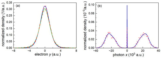
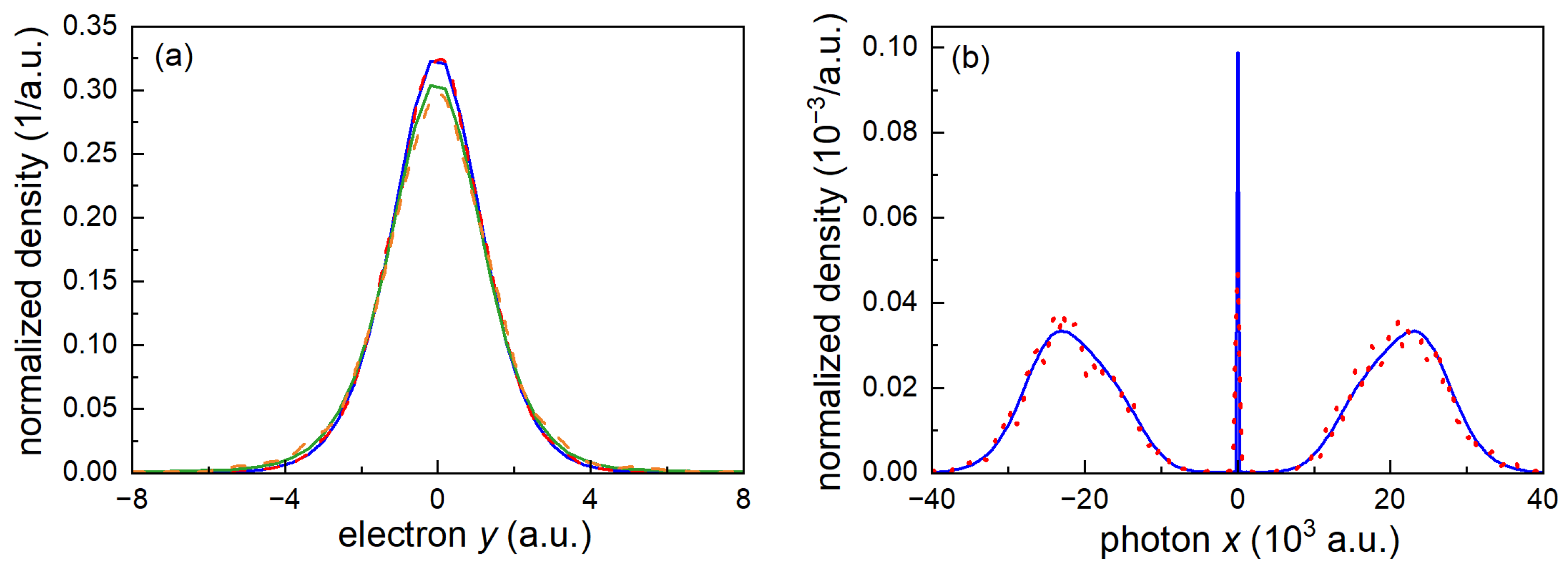
Figure 3 compares the spatial profiles of the electron and of the photon at the end of the pulse, obtained from the solution of Equations (22) and (23), with kernel density estimates (KDE) over the Metropolis walkers. The electron density with and without a photon, the electron density in the one-photon component and the photon profile of the packets are reproduced within the statistical noise. The two electron profiles nearly coincide (Figure 3a). The core of the photon distribution at the atom is narrower than the kernel and is not resolved by the estimate.
Figure 3.
Normalized spatial profiles at the end of the pulse, from the solution of Equations (22) and (23) (solid lines) and from kernel density estimates over the walkers (broken lines). (a) Electron density with and without a photon (blue solid; estimate over all walkers, red dashed) and in the one-photon component, (green solid; estimate over the walkers with a photon, orange dashed). (b) Photon number density (blue solid; estimate over the walkers with a photon, red dotted); the narrow peak at the atom is the photon cloud of the dressed vacuum. All profiles are normalized to one.
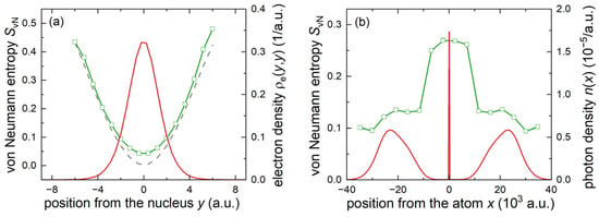
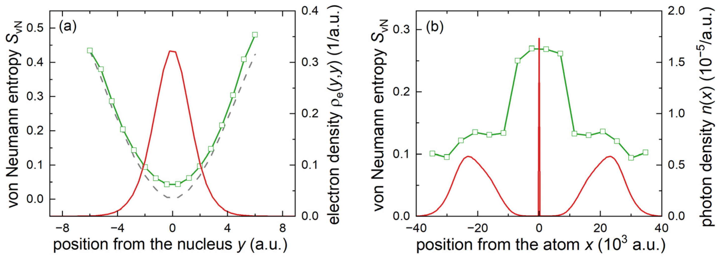
Figure 4 shows the local von Neumann entropies of the strips at the end of the pulse and in the dressed ground state. The two particles show opposite patterns. The electron entropy has its minimum at the nucleus () and grows with the distance from it, to at , while the photon entropy is largest near the atom, , where photons are created and absorbed (), and smaller in the outgoing packets ( to ). The cloud at the atom is one photon grid cell wide (Figure 3b), so the photon entropy there is an average over this cell, whereas the outgoing packets are resolved. With , and strips the strip that contains the atom has the entropy , and , and the packets stay between and ; the narrowest strips show larger values at the sparsely populated edges of the cloud. Both patterns originate in the dressed ground state, in which the photon is confined to the cloud at the atom (strip entropy ), and they follow from the form of the coupling. Equations (22) and (23) contain no potential that depends on the distance between the electron and the photon; their coordinates do not even refer to the same direction. The coupling converts the component without a photon into the one-photon component and back, with an amplitude that factorizes into the dipole lever arm of the electron and the field profile at the atom.
Figure 4.
Local von Neumann entropies of the strips. (a) Electron strips at the end of the pulse (green) and in the dressed ground state at (grey, dashed), as a function of the position measured from the nucleus; electron density (red, right axis). (b) Photon strips at the end of the pulse (green), as a function of the position along the guide, measured from the atom; photon number density (red, right axis). In the dressed ground state the photon is confined to the cloud at the atom, whose strip has the entropy , and the electron strips have their minimum at the nucleus (). The statistical error, estimated from six independent samples of walkers, is at most for the electron strips and for the photon strips.
To first order in the coupling, the photon state conditioned on the electron at , Equation (30), consists of the vacuum and a photon cloud at the atom whose amplitude is proportional to the electron position. Its one-photon part changes sign with ; electrons on the two sides of the nucleus come with photon clouds of opposite sign, and the RDM of a photon strip at the atom mixes these different states. A photon in an outgoing packet has left the region in which acts. Its shape was fixed at the time of emission, and after coherent scattering the electron state that goes with it does not depend on the position of the photon, as seen in Figure 1b and Figure 3a. The local entanglement of the photon is therefore concentrated where photons are created and absorbed, and that of the electron is concentrated where its dipole coupling is strong.
4. Conclusions
We have written the photon-number hierarchy of nonrelativistic QED in the configuration space of the photons, in the length gauge, starting from Fermi’s oscillator representation of the field. In this form, the photon has a coordinate of its own and is created around the atom with the nonlocal kernel , and the state of the electrons and the field is a sequence of wave functions in configuration spaces whose dimension changes with the photon number. Truncated at one photon, the equations call for a sector-dependent treatment of the polarization energy, which we keep only in the component without a photon; with this approximation, the entanglement induced by the pulse converges with the cutoff. We solved the equations without the rotating-wave approximation for a one-dimensional model atom in a waveguide with a single transverse mode, driven by a short off-resonant laser pulse, with the electron, including its continuum, and the photon on real-space grids. Avoiding the RWA has two advantages. The counter-rotating terms create the photon cloud of the dressed ground state and are not negligible for an off-resonant drive, and no transition frequency is needed to define a rotating frame, which allows the atom to keep all its bound states and its continuum.
During the pulse, the atom emits a photon into the guide with probability . The global electron–photon entanglement rises from its value in the dressed ground state to a maximum shortly after the peak of the pulse and then falls because the polarized electron cloud returns to the core, and the electron states that accompany the components with and without a photon become nearly the same. After the pulse, the state is close to a product of the electron state and a superposition of the field vacuum with one scattered photon. The local entanglement, obtained from walkers sampled over both photon-number components, shows opposite patterns for the two particles. The electron entropy is smallest at the nucleus and grows with the distance from it, as a map of the local strength of the dipole coupling, while the photon entropy is largest near the atom, where photons are created and absorbed, and small in the outgoing packets, whose shape was fixed at the time of emission. The entropies refer to the partition between the electron and the transverse field of the length gauge and are not gauge-invariant quantities. Far from the atom, this field coincides with the electric field, and we expect the transient character of the global entanglement and the small entanglement of the outgoing packets to survive a change in partition, while the values near the atom, including those of the dressed ground state, depend on it. The one-dimensional system considered here serves as a demonstration, while the equations of Section 2.1, Section 2.2, Section 2.3, Section 2.4 and Section 2.5 apply, in the dipole approximation, to many electrons in three dimensions.
With the basic equations and the solution method established and tested here, the primary next goal is to extend the number of atoms and photons to realistic values within time-dependent quantum Monte Carlo, in which the photons, like the electrons, are represented by walkers and guide waves, and the photon number becomes an additional variable of the walker; chains and lattices of atoms coupled to a common field are natural first systems, and arrays of artificial atoms in superconducting waveguides are a natural testbed for them [38]. Further extensions are two-dimensional geometries, in which the photon cloud acquires the full tail of , and the two-photon component, which already at the field used here raises the entanglement induced by the pulse. A dispersive guide requires only a different photon energy in the propagation, while absorbing and open structures call for the medium-assisted field of macroscopic QED [40], in which the Fock components can in principle be written in the same form, with the photon labels replaced by those of the excitations of the field and the medium. For few-level emitters, matrix-product-state methods already treat many photons in waveguide QED [16,38,41,42]; the configuration-space approach is aimed at emitters with real-space electronic structure, including the continuum, and at many electrons. Entanglement between an emitter and the photon it emits has been observed for a superconducting qubit and an itinerant microwave photon [43]. That experiment involves a two-level emitter and does not resolve the photon in space, unlike the model considered here.
Funding
This research is based upon work supported by the Bulgarian Ministry of Education and Science as a part of the National Roadmap for Research Infrastructure, grant DO1-102/25.06.2025 (ELI ER-IC BG), and by the National Science Fund, grant KП-06-H78/6.
Institutional Review Board Statement
Not applicable.
Informed Consent Statement
Not applicable.
Data Availability Statement
The data presented in this study are available on request from the author.
Conflicts of Interest
The author declares no conflicts of interest.
References
- Dirac, P.A.M. The quantum theory of the emission and absorption of radiation. Proc. R. Soc. Lond. A 1927, 114, 243–265. [Google Scholar] [CrossRef] [Scilit]
- Heisenberg, W.; Pauli, W. Zur Quantendynamik der Wellenfelder. Z. Phys. 1929, 56, 1–61. [Google Scholar] [CrossRef] [Scilit]
- Fermi, E. Quantum Theory of Radiation. Rev. Mod. Phys. 1932, 4, 87–132. [Google Scholar] [CrossRef] [Scilit]
- Grangier, P.; Roger, G.; Aspect, A. Experimental Evidence for a Photon Anticorrelation Effect on a Beam Splitter: A New Light on Single-Photon Interferences. Europhys. Lett. 1986, 1, 173–179. [Google Scholar] [CrossRef] [Scilit]
- Kimble, H.J.; Dagenais, M.; Mandel, L. Photon Antibunching in Resonance Fluorescence. Phys. Rev. Lett. 1977, 39, 691–695. [Google Scholar] [CrossRef] [Scilit]
- Haugland, T.S.; Ronca, E.; Kjønstad, E.F.; Rubio, A.; Koch, H. Coupled cluster theory for molecular polaritons: Changing ground and excited states. Phys. Rev. X 2020, 10, 041043. [Google Scholar] [CrossRef] [Scilit]
- Weight, B.M.; Tretiak, S.; Zhang, Y. Diffusion quantum Monte Carlo approach to the polaritonic ground state. Phys. Rev. A 2024, 109, 032804. [Google Scholar] [CrossRef] [Scilit]
- Landau, L.; Peierls, R. Quantenelektrodynamik im Konfigurationsraum. Z. Phys. 1930, 62, 188–200. [Google Scholar] [CrossRef] [Scilit]
- Fock, V. Konfigurationsraum und zweite Quantelung. Z. Phys. 1932, 75, 622–647. [Google Scholar] [CrossRef] [Scilit]
- Fock, V. Zur Quantenelektrodynamik. Phys. Z. Sowjetunion 1934, 6, 425–469, English Translation: On Quantum Electrodynamics. In V.A. Fock—Selected Works: Quantum Mechanics and Quantum Field Theory; Faddeev, L.D., Khalfin, L.A., Komarov, I.V., Eds.; Chapman & Hall/CRC: Boca Raton, FL, USA, 2004; pp. 331–368. [Google Scholar]
- Białynicki-Birula, I. Photon wave function. Prog. Opt. 1996, 36, 245–294. [Google Scholar] [CrossRef] [Scilit]
- Sipe, J.E. Photon wave functions. Phys. Rev. A 1995, 52, 1875–1883. [Google Scholar] [CrossRef] [Scilit] [PubMed]
- Smith, B.J.; Raymer, M.G. Photon wave functions, wave-packet quantization of light, and coherence theory. New J. Phys. 2007, 9, 414. [Google Scholar] [CrossRef] [Scilit]
- Keller, O. On the theory of spatial localization of photons. Phys. Rep. 2005, 411, 1–232. [Google Scholar] [CrossRef] [Scilit]
- Shen, J.-T.; Fan, S. Coherent Single Photon Transport in a One-Dimensional Waveguide Coupled with Superconducting Quantum Bits. Phys. Rev. Lett. 2005, 95, 213001. [Google Scholar] [CrossRef] [Scilit] [PubMed]
- Arranz Regidor, S.; Crowder, G.; Carmichael, H.; Hughes, S. Modeling quantum light-matter interactions in waveguide QED with retardation, nonlinear interactions, and a time-delayed feedback: Matrix product states versus a space-discretized waveguide model. Phys. Rev. Res. 2021, 3, 023030. [Google Scholar] [CrossRef] [Scilit]
- Chan, K.W.; Law, C.K.; Eberly, J.H. Localized Single-Photon Wave Functions in Free Space. Phys. Rev. Lett. 2002, 88, 100402. [Google Scholar] [CrossRef] [Scilit] [PubMed]
- Fedorov, M.V.; Efremov, M.A.; Kazakov, A.E.; Chan, K.W.; Law, C.K.; Eberly, J.H. Spontaneous emission of a photon: Wave-packet structures and atom-photon entanglement. Phys. Rev. A 2005, 72, 032110. [Google Scholar] [CrossRef] [Scilit]
- Bužek, V.; Drobný, G.; Kim, M.G.; Havukainen, M.; Knight, P.L. Numerical simulations of atomic decay in cavities and material media. Phys. Rev. A 1999, 60, 582–592. [Google Scholar] [CrossRef] [Scilit]
- Ligare, M.; Oliveri, R. The calculated photon: Visualization of a quantum field. Am. J. Phys. 2002, 70, 58–66. [Google Scholar] [CrossRef] [Scilit]
- Ivanov, I.A.; Kim, K.T. Entanglement in photo-ionization process. Sci. Rep. 2024, 14, 11378. [Google Scholar] [CrossRef] [Scilit] [PubMed]
- Stammer, P.; Rivera-Dean, J.; Maxwell, A.; Lamprou, T.; Ordóñez, A.; Ciappina, M.F.; Tzallas, P.; Lewenstein, M. Quantum electrodynamics of intense laser-matter interactions: A tool for quantum state engineering. PRX Quantum 2023, 4, 010201. [Google Scholar] [CrossRef] [Scilit]
- Christov, I.P. Time-dependent quantum Monte Carlo: Preparation of the ground state. New J. Phys. 2007, 9, 70. [Google Scholar] [CrossRef] [Scilit]
- Christov, I.P. Dynamic correlations with time-dependent quantum Monte Carlo. J. Chem. Phys. 2008, 128, 244106. [Google Scholar] [CrossRef] [Scilit] [PubMed]
- Christov, I.P. Entanglement islands in 1D and 2D lattices with defects. Entropy 2025, 27, 1093. [Google Scholar] [CrossRef] [Scilit] [PubMed]
- Christov, I.P. Statistics of Marginal Wave Functions as a Real-Space Diagnostic of Quantum Entanglement. ACS Omega 2026, 11, 48373–48383. [Google Scholar] [CrossRef] [Scilit] [PubMed]
- Cohen-Tannoudji, C.; Dupont-Roc, J.; Grynberg, G. Photons and Atoms: Introduction to Quantum Electrodynamics; Wiley: New York, NY, USA, 1989. [Google Scholar]
- Woolley, R.G. Molecular quantum electrodynamics. Proc. R. Soc. Lond. A 1971, 321, 557–572. [Google Scholar] [CrossRef] [Scilit]
- Craig, D.P.; Thirunamachandran, T. Molecular Quantum Electrodynamics: An Introduction to Radiation–Molecule Interactions; Academic Press: London, UK, 1984. [Google Scholar]
- Rokaj, V.; Welakuh, D.M.; Ruggenthaler, M.; Rubio, A. Light–matter interaction in the long-wavelength limit: No ground-state without dipole self-energy. J. Phys. B 2018, 51, 034005. [Google Scholar] [CrossRef] [Scilit]
- Dalibard, J.; Dupont-Roc, J.; Cohen-Tannoudji, C. Vacuum fluctuations and radiation reaction: Identification of their respective contributions. J. Phys. 1982, 43, 1617–1638. [Google Scholar] [CrossRef] [Scilit]
- Glauber, R.J. The Quantum Theory of Optical Coherence. Phys. Rev. 1963, 130, 2529–2539. [Google Scholar] [CrossRef] [Scilit]
- Tamm, I. Relativistic interaction of elementary particles. J. Phys. 1945, 9, 449–457. [Google Scholar]
- Dancoff, S.M. Non-Adiabatic Meson Theory of Nuclear Forces. Phys. Rev. 1950, 78, 382–385. [Google Scholar] [CrossRef] [Scilit]
- Bethe, H.A. The Electromagnetic Shift of Energy Levels. Phys. Rev. 1947, 72, 339–341. [Google Scholar] [CrossRef] [Scilit]
- Karmanov, V.A.; Mathiot, J.-F.; Smirnov, A.V. Systematic renormalization scheme in light-front dynamics with Fock space truncation. Phys. Rev. D 2008, 77, 085028. [Google Scholar] [CrossRef] [Scilit]
- Forn-Díaz, P.; García-Ripoll, J.J.; Peropadre, B.; Orgiazzi, J.-L.; Yurtalan, M.A.; Belyansky, R.; Wilson, C.M.; Lupascu, A. Ultrastrong coupling of a single artificial atom to an electromagnetic continuum in the nonperturbative regime. Nat. Phys. 2017, 13, 39–43. [Google Scholar] [CrossRef] [Scilit]
- Sheremet, A.S.; Petrov, M.I.; Iorsh, I.V.; Poshakinskiy, A.V.; Poddubny, A.N. Waveguide quantum electrodynamics: Collective radiance and photon-photon correlations. Rev. Mod. Phys. 2023, 95, 015002. [Google Scholar] [CrossRef] [Scilit]
- Forn-Díaz, P.; Lamata, L.; Rico, E.; Kono, J.; Solano, E. Ultrastrong coupling regimes of light-matter interaction. Rev. Mod. Phys. 2019, 91, 025005. [Google Scholar] [CrossRef] [Scilit]
- Scheel, S.; Buhmann, S.Y. Macroscopic quantum electrodynamics—Concepts and applications. Acta Phys. Slovaca 2008, 58, 675–809. [Google Scholar] [CrossRef] [Scilit]
- Pichler, H.; Zoller, P. Photonic Circuits with Time Delays and Quantum Feedback. Phys. Rev. Lett. 2016, 116, 093601. [Google Scholar] [CrossRef] [Scilit] [PubMed]
- Peropadre, B.; Zueco, D.; Porras, D.; García-Ripoll, J.J. Nonequilibrium and Nonperturbative Dynamics of Ultrastrong Coupling in Open Lines. Phys. Rev. Lett. 2013, 111, 243602. [Google Scholar] [CrossRef] [Scilit] [PubMed]
- Eichler, C.; Lang, C.; Fink, J.M.; Govenius, J.; Filipp, S.; Wallraff, A. Observation of Entanglement between Itinerant Microwave Photons and a Superconducting Qubit. Phys. Rev. Lett. 2012, 109, 240501. [Google Scholar] [CrossRef] [Scilit] [PubMed]

Disclaimer/Publisher’s Note: The statements, opinions and data contained in all publications are solely those of the individual author(s) and contributor(s) and not of MDPI and/or the editor(s). MDPI and/or the editor(s) disclaim responsibility for any injury to people or property resulting from any ideas, methods, instructions or products referred to in the content. |
© 2026 by the author. Licensee MDPI, Basel, Switzerland. This article is an open access article distributed under the terms and conditions of the Creative Commons Attribution (CC BY) license.