


Abstract
This study evaluates simulated single-round label acquisition for anonymised card-transaction fraud within a software-quality framework. A fixed chronological split, logistic regression and histogram gradient boosting, 30 random seeds, five review budgets, and 12 acquisition policies are used with an ideal label oracle. A 67-setting weight-simplex analysis examines the sensitivity and redundancy of the composite uncertainty, risk and threshold-proximity score. Logistic-regression baseline average precision is 0.5945; the highest mean acquisition AP is 0.6093 for entropy plus threshold proximity at a 5% budget, with unchanged recall and higher illustrative total cost. Histogram boosting is substantially more variable across seeds; its highest mean AP among the 12 core policies is 0.3698, compared with a baseline of 0.3140, and the paired seed interval includes zero. The composite score does not consistently dominate simpler policies or retain an optimal weight across budgets. Binary entropy is theoretically rank-equivalent to predictive ambiguity, rather than an independent information source. Retrospective monitoring applies Holm correction over 180 comparisons per classifier and reports KS effect magnitudes and PSI. All six temporal chunks trigger the specified effect-gated alarm, whereas none of 100 empirical same-source control repetitions per classifier does; this control does not establish prospective specificity. Costs are hypothetical relative penalties, SHAP examples are illustrative, and all empirical conclusions are restricted to a single-dataset proof of concept.
1. Introduction
E-commerce platforms increasingly rely on automated decision systems to screen transactions, monitor accounts, detect abusive behaviour, and protect customers from financial harm. Fraud detection is therefore a central component of digital commerce infrastructures. It is also a difficult machine learning problem: fraudulent events are rare, labels may be delayed or noisy, user and attacker behaviour evolves over time, and business costs are asymmetric. A false negative can lead to direct financial loss, while a false positive can block a legitimate customer, generate manual work, and reduce trust in the service.
Research on fraud detection has produced a large body of work on supervised classification, anomaly detection, deep learning, graph-based modelling, ensemble learning, and cost-sensitive evaluation [1]. These approaches are necessary, but they usually treat fraud detection as a model optimisation problem. In operational settings, however, a fraud detection model is embedded in a larger software and organisational workflow. Alerts are routed to analysts, explanations are consumed by human decision makers, thresholds are adjusted according to risk appetite, and models must be monitored, retrained, audited, and maintained. This means that predictive performance alone is not sufficient for judging the quality of the deployed service.
The problem becomes clearer when considering two alternative systems. A first system may achieve a slightly higher area under the receiver operating characteristic curve (ROC-AUC) but may produce too many low-quality alerts, explanations that analysts cannot act upon, unstable outputs under drift, and a feature pipeline that is difficult to maintain. A second system may have marginally lower model performance but provide calibrated risk scores, interpretable alert evidence, selective human review, and well-defined model update procedures. From a software quality and e-commerce service perspective, the second system may be preferable.
This paper proposes a broader quality-aware fraud-detection framework and evaluates a simulated single-round label-acquisition component on card transactions. The proposed approach brings together three complementary research traditions: machine learning for fraud detection, software quality evaluation for e-commerce systems, and human-centred artificial intelligence. It is motivated by the need to evaluate fraud detection as an AI-enabled decision service whose quality depends on interactions between data, models, explanations, human analysts, software pipelines, and business processes.
This empirical study instantiates selected framework components through a simulated, single-round label-acquisition experiment on anonymised card transactions. This setting connects the broader architecture to measurable predictive, review-yield, and cost outcomes.
The guiding research question is:
How can software quality attributes and human-in-the-loop mechanisms be integrated into machine learning-based fraud detection so that e-commerce systems become more accurate, explainable, maintainable, reliable, and operationally trustworthy?
The paper makes four contributions. First, it proposes a conceptual architecture for quality-aware fraud detection in e-commerce systems. Second, it maps ISO/IEC 25010-inspired software quality characteristics to fraud detection pipeline requirements and measurable indicators. Third, it defines a human-in-the-loop protocol that combines uncertainty-aware case selection, analyst feedback, explainable alerts, and single-round active label acquisition and model update. Fourth, it empirically evaluates selected predictive, review-efficiency, and cost dimensions of the broader quality-aware framework through a reproducible multi-budget and multi-seed experiment. The intended contribution is therefore not a claim that HITL always improves fraud detection or that all ISO/IEC 25010-inspired qualities are empirically measured in the present experiment, but a framework for determining when HITL improves a deployment-relevant quality dimension and when its operational cost is not justified.
The remainder of the paper is organised as follows. Section 2 reviews related work on fraud detection, software quality, explainable AI, and human-in-the-loop learning. Section 3 presents the proposed framework. Section 4 specifies the implemented procedures and evaluation criteria. Section 5 reports empirical results. Section 6 discusses implications, limitations, and future work. Section 7 concludes the paper.
2. Related Work
2.1. Machine Learning for Fraud Detection
Fraud detection has long been studied as a classification and anomaly detection problem in finance, telecommunications, insurance, and e-commerce [2,3]. Traditional approaches include logistic regression, decision trees, support vector machines, random forests, gradient boosting, neural networks, and hybrid ensemble models [4,5]. The predictive task is complicated by class imbalance: fraudulent transactions represent a small minority of all transactions, which makes standard accuracy misleading [6,7]. As a result, fraud detection studies typically use precision, recall, F1-score, ROC-AUC, precision–recall curves, cost-sensitive evaluation, or top-ranked alert measures [8,9,10].
Tree-based methods remain strong baselines for tabular transaction data because they handle heterogeneous features, nonlinear interactions, and variable importance estimation. Random forests [11] and gradient boosting systems such as XGBoost [12] are widely used in high-performing tabular classification pipelines. Prior work on realistic credit-card fraud modelling also highlights the importance of temporal validation, alert capacity, delayed feedback, and combinations of supervised and unsupervised learning [13,14,15]. Deep learning approaches can be useful when fraud signals are embedded in sequential, graph, behavioural, or multimodal data, although they often require a greater data volume and raise additional interpretability and maintenance concerns [16].
Recent work addresses operational requirements alongside predictive accuracy. Cao et al. propose iTA-LRN, combining transaction-sequence modelling with monitoring and incremental model updates [17]. Zhu et al. introduce DISCO, separating representation learning from conformal risk control of the false-negative rate under its statistical assumptions [18]. These approaches motivate distinguishing adaptation and risk control from aggregate discrimination. The present study instead isolates budgeted, single-round label acquisition with two tabular classifiers; it does not evaluate sequence modelling, incremental deployment or conformal risk guarantees.
The deployment of fraud detection systems introduces additional difficulties. Labels may arrive only after chargeback investigation or customer dispute resolution. Model training data may be affected by prior fraud rules and analyst decisions, creating feedback loops. Fraud strategies may change intentionally in response to detection mechanisms. Thus, a system that performs well on a static benchmark may degrade in production if it is not monitored and updated.
2.2. Software Quality in E-Commerce Systems
Software quality evaluation provides a systematic vocabulary for analysing whether a system satisfies explicit and implicit requirements. The ISO/IEC 25010:2011 product quality model comprises functional suitability, performance efficiency, compatibility, usability, reliability, security, maintainability, and portability [19]. That edition supplies the terminology used in the framework mapping. The 2023 edition defines a revised, nine-characteristic product quality model [20]; the two editions are therefore distinguished rather than treated as identical taxonomies. These characteristics are directly relevant to e-commerce because system failures can affect revenue, customer trust, regulatory compliance, and service continuity.
Previous work on e-commerce quality has examined web metrics, user-centred characteristics, service effectiveness, and quality models for complex information systems [21,22]. This line of work is important for AI-enabled fraud detection because fraud screening is not merely an analytical component. It is part of an e-commerce service that interacts with checkout, payments, customer service, risk operations, and business reporting.
When machine learning is introduced, quality characteristics require reinterpretation. Reliability includes not only uptime but also robustness to concept drift and calibration stability. Maintainability includes feature pipeline traceability, reproducible model training, monitoring coverage, and retraining effort. Usability includes whether human analysts can understand alert evidence and make timely decisions. Security includes both data protection and resilience to adversarial behaviour. These concerns are consistent with production ML quality work on testing, monitoring, data dependencies, and operational readiness [23,24].
2.3. Explainable and Human-Centred AI
Explainable artificial intelligence (XAI) methods aim to make model outputs more understandable to human users [25,26]. Local explanation techniques, such as LIME [27] and SHAP [28], are commonly used to identify features that influence individual predictions. In fraud detection, explanations can support analyst review by indicating suspicious transaction attributes, unusual account behaviour, or risk-contributing features.
However, the mere presence of an explanation does not guarantee improved decision quality. Explanations may be too complex, unstable, misleading, or unrelated to the analyst’s operational question. For this reason, explanation quality should be evaluated from both computational and human-centred perspectives, and in high-stakes domains there is an active debate over when interpretable models should be preferred to post hoc explanations [29,30]. Relevant properties include fidelity, stability, sparsity, actionability, consistency, and perceived usefulness.
Human-in-the-loop machine learning introduces human feedback into the model lifecycle [31,32]. In fraud detection, humans may confirm alerts, correct false positives, label uncertain cases, adjust thresholds, review high-value transactions, and identify emerging fraud patterns. In iterative settings, active learning can help select the most informative cases for review, reducing labelling effort while improving model updates [33]. From a software engineering perspective, human-in-the-loop ML also raises requirements for workflow design, traceability, monitoring, and accountability [34,35].
Recent human-centred XAI evaluation work distinguishes contextual explanation quality, human–AI interaction, and joint performance [36]. This distinction supports using computational attribution as a limited diagnostic and reserving claims about analyst usefulness for a user study. Together with the fraud-detection literature, it provides a basis for distinguishing model explanations from human-centred validation.
A systematic review and meta-analysis by Vaccaro et al. finds that human–AI combinations do not, on average, outperform the better of the human-only and AI-only alternatives, with substantial variation across settings [37]. This evidence motivates evaluating collaboration against appropriate standalone baselines. In the present ideal-oracle simulation, acquired labels allow a computational comparison with the model baseline but do not measure human–AI complementarity; that would require a controlled analyst study.
2.4. Research Gap
Existing studies often optimise fraud detection models according to predictive metrics, while software quality studies often evaluate e-commerce systems without detailed integration of machine learning lifecycle concerns. At the same time, XAI studies frequently assess explanations without embedding them in a full operational quality framework. The resulting gap is a lack of methods for evaluating fraud detection as an AI-enabled e-commerce service.
This paper addresses that gap by proposing a framework in which fraud detection performance, software quality, explainability, and human feedback are considered within a common evaluation structure. The present experiment operationalises selected predictive, review-efficiency, computational attribution-diagnostic, and cost dimensions of this structure. The aim is not to replace predictive evaluation but to enrich it with quality attributes that matter in real deployment.
3. Proposed Quality-Aware Framework
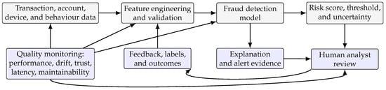
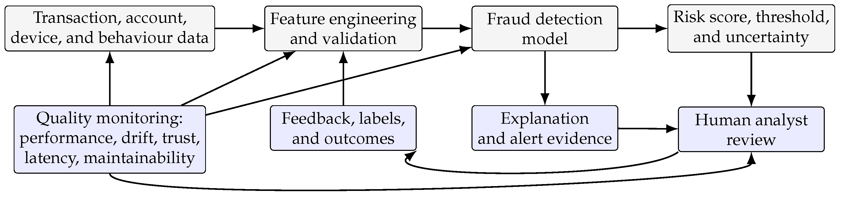
The proposed framework views fraud detection as a layered decision service. Figure 1 presents the conceptual architecture. It contains five interacting layers: data and feature management, predictive modelling, explanation and uncertainty estimation, human review and feedback, and quality monitoring.
Figure 1.
Conceptual architecture of the quality-aware human-in-the-loop fraud detection framework. Arrows indicate data, prediction, review, feedback and monitoring flows. Grey boxes represent the predictive pipeline; blue boxes represent explanation, human review, feedback and quality monitoring.
3.1. Design Principles
The framework is based on five design principles:
- Predictive performance is necessary but insufficient. A high-performing classifier may still be unsuitable if it produces excessive false positives, unstable alerts, or explanations that analysts cannot use.
- Quality attributes should be explicit. Reliability, usability, maintainability, security, and performance efficiency should be represented by measurable indicators in the fraud detection pipeline.
- Human attention should be allocated selectively. Analyst review should focus on uncertain, high-risk, high-value, novel, or strategically informative cases.
- Explanations should support action. Alert explanations should be evaluated by their ability to help analysts understand, validate, and document decisions.
- Feedback should drive continuous improvement. Analyst outcomes should feed labelling, retraining, drift analysis, threshold selection, and rule refinement.
3.2. Quality Characteristics and Fraud Detection Indicators
Table 1 maps selected software quality characteristics to fraud detection concerns and measurable indicators. The mapping adapts ISO/IEC 25010-inspired concepts to AI-enabled fraud detection services. The final column distinguishes measured outcomes from framework requirements. The indicative measures are candidate deployment measures, not a claim that every listed indicator was calculated. Table 1 is an ISO/IEC-inspired mapping, not a compliance assessment; the older and revised standards use different quality taxonomies.
Table 1.
Mapping between software quality characteristics and fraud detection indicators.
3.3. Quality-Aware Decision Flow
The proposed decision flow combines automated scoring with selective review. For each transaction , a model produces a fraud probability and an uncertainty score . In the conceptual decision rule, lower and upper action thresholds and define automatically accepted and automatically held regions, while defines the minimum uncertainty level that triggers review. A decision policy then determines whether the transaction should be accepted, rejected, or escalated for human review:
Here, and are conceptual decision-band thresholds, and is a conceptual threshold on the uncertainty score . They describe a general production policy for accept/reject/review routing. The empirical experiment uses a single deployed alert threshold for threshold selection and for the threshold-proximity component below; therefore, should not be confused with the conceptual pair . In production, the human review set can be further prioritised using expected financial value, customer segment, novelty, or disagreement between the model and existing business rules. In the reported experiment, however, review priority is operationalised only through the implemented uncertainty (U), risk (R), and threshold-proximity (T) components. This design allows the system to reserve analyst effort for cases where human judgement is likely to add value while keeping the empirical policy definition reproducible.
For the quality-aware policy, review priority is defined through a composite review score. Let denote the single operational alert threshold used in the empirical deployment simulation, and let B denote the number of cases that can be reviewed under a fixed analyst budget. In the experiment, is not fixed at 0.5 and does not represent the conceptual low/high threshold pair in the decision rule above. It is selected as the validation-score 99th percentile under a researcher-defined 1% alert-capacity scenario. This selects an operating threshold; it does not calibrate probabilities. For each candidate transaction , the model produces an uncalibrated predicted fraud score . The raw uncertainty component used both in the conceptual decision rule and in the implemented review score is defined as
so that transactions near the probabilistic classification boundary receive higher uncertainty values. This component captures model ambiguity around and is independent of the operational alert threshold. The raw risk and threshold-proximity components are defined as
Threshold proximity differs from uncertainty because it measures closeness to the deployed operating point , not closeness to 0.5. Under severe class imbalance and a fixed alert-rate policy, can be substantially different from 0.5; therefore and may rank different transactions. To make the components comparable before linear aggregation, each component is min–max normalised over the candidate review window:
Constant or numerically near-constant components are set to zero using the default NumPy isclose comparison; otherwise, the displayed min–max expression is used. The quality-aware review score is then
The review set contains the top B priorities, with smaller original CSV row IDs resolving ties. The reference weights are a transparent heuristic, not an estimate of financial severity or an optimised operating rule. The components are deterministic transformations of the same predicted score and do not constitute independent evidence. A systematic analysis evaluates all 66 triples in increments of 0.1 on the nonnegative unit simplex and the reference triple at every budget and seed. This analysis characterises sensitivity rather than tuning weights on the future hold-out. Pearson and Spearman correlations, selected-set overlap and the number of distinct selections complement predictive and cost comparisons.
3.4. Information-Theoretic Analysis
Let , with . Predictive entropy is . Numerical evaluation clips to . Because probabilities are not calibrated, measures uncertainty under the fitted predictive distribution; it is not an estimate of the true conditional entropy of fraud labels.
Proposition 1
(Binary rank equivalence). For , predictive entropy satisfies
The mapping is strictly increasing for , so entropy-only and uncertainty-only acquisition have identical rankings, including theoretical ties. Proof. and binary entropy is symmetric. Furthermore,
Clipping can merge numerical ties at extreme probabilities. Thus, entropy contributes an interpretable unit and nonlinear rescaling, not independent acquisition evidence. Composite entropy scores can change rankings because is nonlinear; such changes do not establish a new source of information.
Proposition 2
(Entropy allocation identity and bound). For a candidate window of N transactions with positive total entropy, a selected set A of B cases has mean-entropy enrichment and entropy-mass coverage . Therefore,
Selecting the top B entropies maximises at fixed B. Its coverage obeys . Proof. The identity follows by dividing selected and total sums by their counts. Replacing any selected entropy by a larger omitted entropy increases the selected sum. The mean of the largest B values is at least the overall mean, and each entropy is at most one bit, yielding both bounds. These are elementary consequences of binary entropy, not claims of novel general information theory [38,39].
Enrichment and entropy-mass coverage are algebraically linked diagnostics, not independent confirmations. Proposition 2 describes the analytical consequence of top-entropy selection; no empirical entropy-concentration percentage is claimed for the present experiment. Neither proposition implies more fraud labels, fewer false negatives or improved future AP. Proposition 1 concerns exact mathematical score functions; finite-precision evaluation and clipping are implementation details considered explicitly in the acquisition methods and numerical results.
Proposition 3
(Idealised noisy-label information). Suppose, for analysis only, that the true fraud probability is p and an analyst label independently flips the true binary label with probability . The information provided about that label is
Proof. The observed-label probability is , while uses the mutual-information identity. Perfect feedback () reveals bits about the selected label, whereas uninformative feedback () reveals zero. This model exposes the ideal-oracle assumption in the experiment. It is an analytical scenario, not an empirically estimated analyst error model. Label-specific information is distinct from information about model parameters or future transactions; learning benefit also depends on representativeness, redundancy, calibration, and update dynamics. Accordingly, the manuscript does not equate selected predictive entropy with expected model improvement.
4. Materials and Methods
4.1. Study Scope and Evaluation Criteria
This study evaluated simulated single-round label acquisition on one anonymised credit-card benchmark. The conceptual architecture defined deployment requirements; the experiment measured predictive discrimination, thresholded errors, review yield, hypothetical cost, computational attribution and retrospective distribution monitoring. P1 denoted a fitted baseline classifier. P2 added explanations without altering its predictions. P3 acquired selected review-window labels and fitted a new classifier once. No analysts participated.
The empirical questions were whether acquisition reduced future false positives at the validation-defined operating point (H1) and whether the composite score improved label yield over random or single-component selection at matched budgets (H2). Label yield was , with acquired fraud labels; enrichment was . Learning benefit was separately assessed through future average precision (AP). Here, PR-AUC was computed as AP, rather than trapezoidal integration. A high label yield did not imply improved future predictions or lower cost. Design propositions about analyst support (D1), monitoring (D2) and maintainability (D3) motivated the framework; D1 and D3 were not tested as human or organisational outcomes.
4.2. Dataset and Chronological Split
The public TensorFlow-hosted creditcard.csv contains 284,807 transactions and 492 fraud labels. Predictors are Time, Amount and V1–V28; Class is the outcome. Source and original row-ID bookkeeping columns were excluded from fitting. Missing values were absent. Data were stably sorted by Time and original CSV row ID, then divided at positional indices 170,884, 227,845 and 256,326. Equal-time ordering was therefore deterministic. The split was based on transaction counts, not fixed time intervals. Table 2 summarises the subsets.
Table 2.
Chronological evaluation subsets.
The few future fraud cases limited inference: one additional detected fraud changed recall by . The input SHA256 and exact split counts are provided with the Supplementary Files.
4.3. Classifiers and Recorded Software Environment
Logistic regression used a StandardScaler fitted only on the applicable training set, L2 regularisation with , the lbfgs solver, balanced class weights, a tolerance of and at most 1200 iterations. Histogram gradient boosting used unscaled inputs, a log loss, learning rate of 0.06, at most 180 iterations, 31 leaves, a minimum of 20 observations per leaf, 255 bins, no depth limit, no class weighting and zero L2 penalty. Automatic early stopping used a 0.1 internal validation fraction, loss scoring, 10 non-improving iterations and a tolerance of . Complete effective parameter dictionaries were archived. There was no imputation, feature selection, additional probability calibration, oversampling or undersampling. Upstream anonymisation of V1–V28 was not fitted here.
The executed environment was Python 3.13.16, NumPy 2.1.3, pandas 2.2.3, SciPy 1.16.3, scikit-learn 1.6.1, Matplotlib 3.10.0, SHAP 0.52.0 and numba 0.61.2 on Linux x86_64. Numerical thread pools were limited to one. The experiment used seeds . Initial fits used the listed seed; acquired-label fits used that seed plus 1000. Software versions and full parameters are supplied in machine-readable files and Supplementary Implementation Settings.
4.4. Operating Point and Acquisition Policies
The threshold was the linearly interpolated 99th percentile of baseline validation probabilities, , with alerts defined by . This selected an operating point and did not calibrate probabilities. The 1% target and budgets were researcher-defined capacity scenarios. Ties and temporal change may have altered realised alert rates.
Budgets were 0.25%, 0.5%, 1%, 2% and 5% of the review window, giving acquired labels. Baseline review probabilities determined every acquisition score. Raw , and were min–max scaled separately over the review window, with numerically constant components set to zero. Single-component policies used these scores; pairwise policies used equal-weight averages; used . They measured ambiguity, predicted fraud likelihood and operating-threshold proximity, respectively. Predictive ambiguity did not isolate epistemic uncertainty, and likelihood was not a transaction-specific financial loss.
Four entropy policies completed the 12-policy comparison. used probabilities clipped to and was not min–max scaled. and used weights 0.55/0.45 with scaled R and T; used 0.45/0.35/0.20. These definitions were fixed across both classifier families. Although U and H were rank-equivalent in exact arithmetic, clipped entropy and floating-point transformations could create or resolve ties differently. Deterministic sorting resolved ties within the computed score; it did not guarantee that two numerically different score functions produced identical tied sets.
Score-based selection used descending computed priority followed by ascending original row order. Random selection sampled without replacement using default_rng(seed), reinitialised at each budget and classifier. Thus, the same random sample was shared between classifier families at a fixed seed and budget, but samples across budgets were not guaranteed to be nested.
4.5. Single-Round Update and Outcome Measures
An ideal oracle revealed the stored labels of selected review transactions without noise, delay or analyst error. These observations were appended to the initial training set, and a fresh estimator was fitted. Logistic scaling and class weights were re-estimated. The 99th-percentile threshold was selected again on the original validation window, which preceded the acquired observations. This was an offline operating-point comparison, not a production simulation with continuously updated thresholds. Future labels did not influence fitting or acquisition.
Future evaluation reported precision, recall, F1, ROC-AUC, AP, alerts, FPs and FNs. Acquired-fraud counts, yield and enrichment were measured on the review window. The main illustrative cost was , in arbitrary common units. Label acquisition in the earlier review window and classification outcomes in the future window referred to distinct transactions; the total was not a return-on-investment estimate.
4.6. Seed Variability and Weight Sensitivity
The core experiment contained result rows: P1 and P2 plus 60 acquired-label conditions for each model–seed pair. Paired AP and cost differences were calculated against the same-seed baseline. Percentile intervals used 20,000 bootstrap resamples of the 30 paired differences with NumPy seed 20260827. Exploratory sign-flip summaries used 100,000 random sign vectors, the add-one Monte Carlo correction and seed 20261015. They were not corrected across acquisition configurations and were not treated as confirmatory evidence. Constant deterministic differences are reported as repeated-run constants, without inferential interpretation.
These summaries characterised algorithmic variation on a fixed hold-out, not population uncertainty. In particular, changing the seed of the deterministic logistic regression did not create 30 independent estimates of performance. Histogram boosting varied partly through its internal early-stopping validation split. The benchmark and future window remained the same in all runs.
The systematic sensitivity grid comprised 66 simplex triples with step 0.1 plus the reference triple, yielding weight-result rows. Identical selected sets reused one augmented fit within each model, seed and budget; all weight rows remained recorded. Pearson and Spearman correlations assessed different aspects of score dependence. Jaccard overlap compared each selected set with the reference weights at the same budget. Distinct-set counts quantified decision redundancy directly. The range of mean AP over weights was descriptive; no weight was selected as a deployable optimum using the hold-out.
4.7. Computational Attribution Diagnostics
Permutation importance used the logistic-regression seed-11 baseline, 6000 sampled future transactions, AP scoring, five repetitions and random state 42. It was a post hoc interpretation diagnostic and never selected fitting or monitoring features. For each baseline classifier at seed 11, local SHAP covered the five highest-score true-fraud alerts and five highest-score false-positive alerts. This small, outcome-conditioned extreme-case sample was illustrative rather than representative. Permutation SHAP attributed positive-class probabilities relative to 100 training-background observations sampled with random state 20260827; the explainer seed was 20261015, and its budget was evaluations per case for predictors.
No user study tested explanation usefulness. The attributions did not establish faster or more accurate human decisions, reduced workload, improved trust, causal fraud mechanisms, fidelity, stability or actionability. Anonymised V features also constrained semantic interpretation.
4.8. Monitoring and Empirical No Drift Control
Baseline seed-11 models scored the validation reference and six chronological future chunks. The first five chunks contained 4747 transactions each and the last 4746. Monitoring features were predefined as V1–V28 and Amount, plus the model score. Time remained a classifier predictor but was excluded from feature alarms because clock time shifted by construction. Future labels did not select monitoring features.
Each variable–chunk comparison recorded the two-sided asymptotic KS statistic D and p-value, and PSI using ten validation-quantile bins. Duplicate edges were removed, endpoint bins extended to infinity and proportions were floored at . The Supplemental Code specifies the degenerate-bin fallback. Holm correction was applied jointly to the p-values within each classifier. The main retrospective alarm required adjusted and , or PSI . Alternative D gates 0.02 and 0.10 characterised sensitivity. The PSI branch was an effect threshold, not a multiplicity-adjusted test. These gates were scenario choices rather than validated deployment thresholds.
For each classifier, 100 control repetitions independently sampled reference and six monitoring sets with replacement from the validation empirical distribution, matching the temporal sample sizes. Random seed 20261015 was reused for each classifier, so their feature-control draws were shared; they were not 200 independent operational experiments. Holm correction was repeated within each control family. Outputs recorded family-level significance-only alarms and combined effect-gated alarms. The control approximated an iid same-source null, not temporal dependence or production specificity. Large samples, tied or discrete scores, and serial dependence limited classical KS interpretations. Statistical marginal shifts did not establish changes in or predictive degradation. The six-chunk Holm family was retrospective; it did not define an online sequential false-alarm guarantee.
5. Results
The experiment yielded 120 acquisition-condition means, 3720 core result records, 20,100 weight-sensitivity records and 36,360 monitoring comparisons. Complete results are provided in the Supplementary Materials. The reference-weight sensitivity analysis agreed with the corresponding composite-policy results across all 300 model–seed–budget combinations.
5.1. Baseline Performance and Acquisition Outcomes
Table 3 reports baseline performance. The logistic-regression baseline had a mean AP of 0.5945, recall of 0.7727, 197 FPs and five FNs, with a cost of 1485 in the main hypothetical scenario. Histogram boosting had a mean AP of 0.3140, recall of 0.6182, 215.7 FPs and 8.4 FNs, with a cost of 1918.7. Baseline HGB’s AP varied from 0.0935 to 0.5890 across seeds (SD 0.1243); logistic regression’s baseline AP was constant. P2 added computational explanations and left P1 predictions unchanged.
Table 3.
Baseline means over 30 seeds on the fixed future window. P2 has identical predictions to P1.
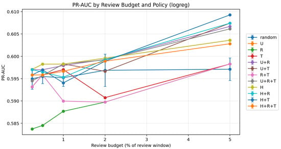
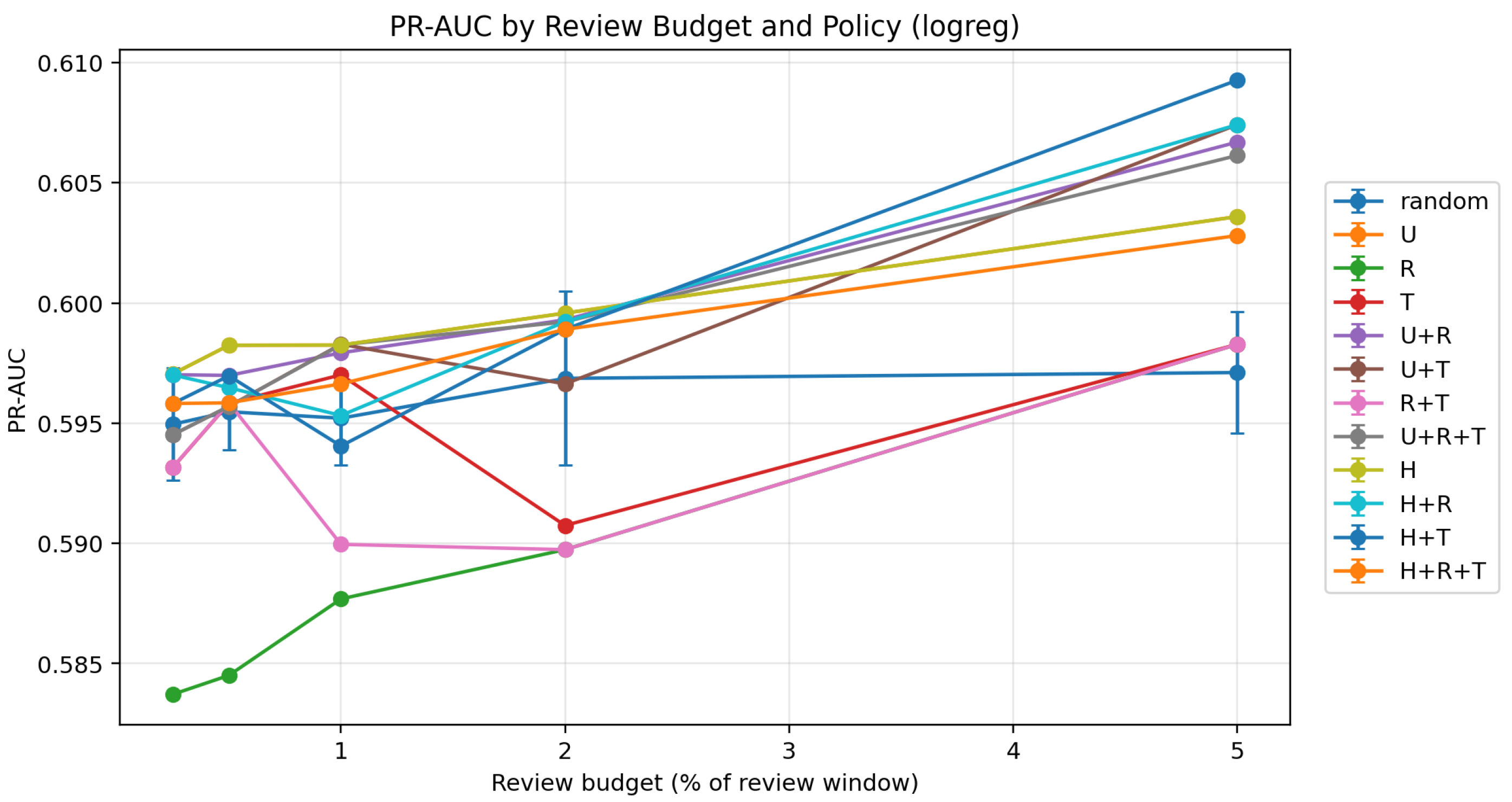
Selected acquisition settings are shown in Table 4; all conditions are in Supplementary Table S1. The highest LR mean AP is 0.6093 for at 5%, compared with 0.6067 for and 0.6061 for . LR recall remains 0.7727 across the core acquisition experiment. The best AP setting leaves FPs unchanged at 197 and raises hypothetical cost to 2909 because it acquires 1424 labels. Thus, its AP increase does not demonstrate fewer missed frauds or cost savings. At 5%, reduces FPs from 197 to 193, but the total cost is 2889.
Table 4.
Selected acquisition settings, means over 30 seeds. Budget is a percentage of the review window; E is fraud enrichment.
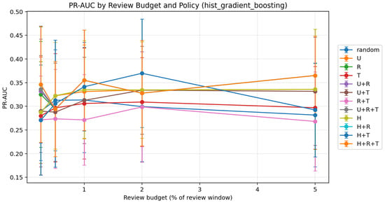
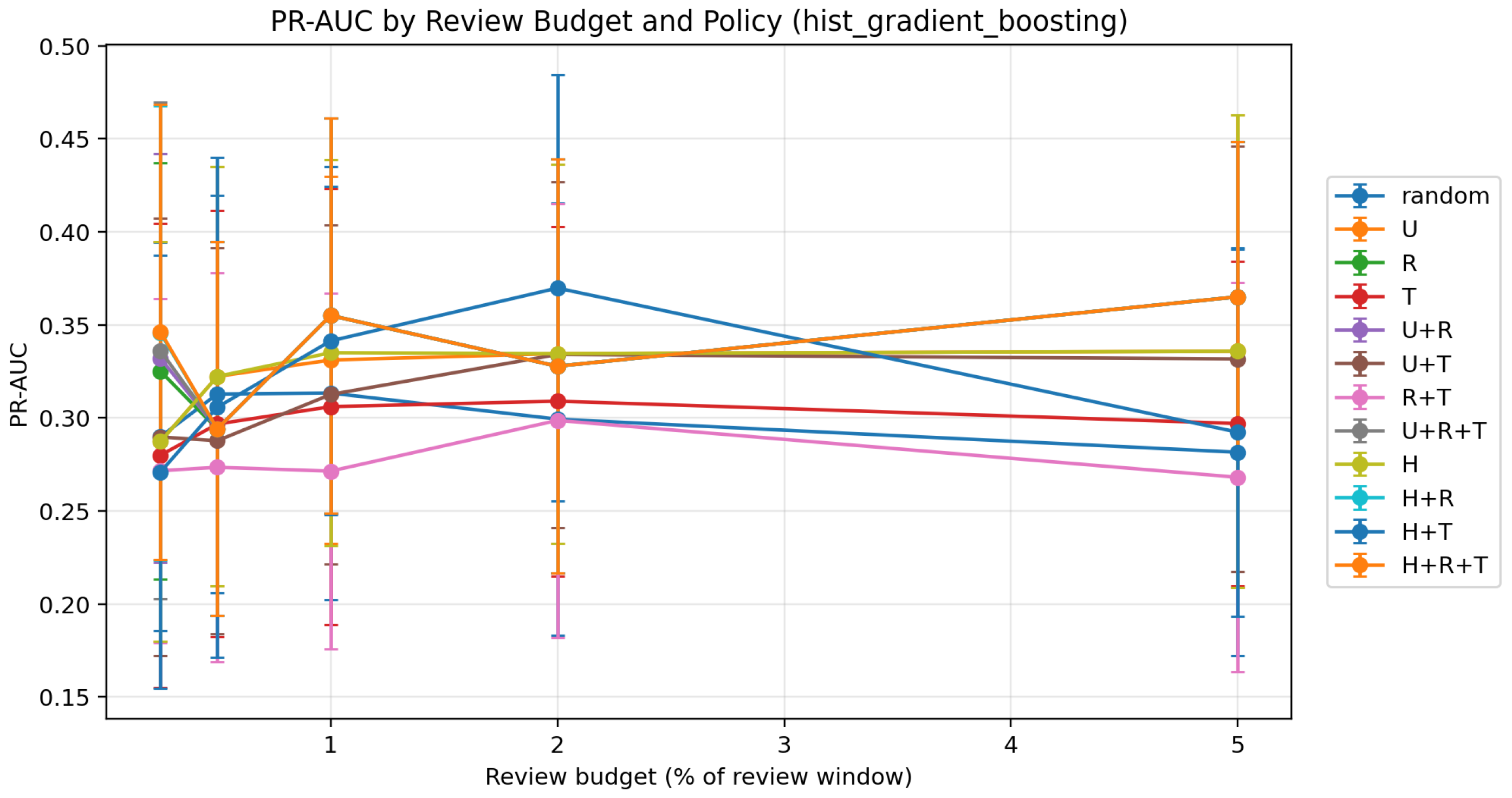
The highest mean acquisition AP among HGB core policies is 0.3698 for at 2%, with a recall of 0.6303, 211.3 FPs and cost 2438.8. At 5%, R, , , and have the same aggregate performance: AP 0.3651, recall 0.6621, 296.1 FPs and cost 3647.7. Increased review volume can therefore improve some discrimination summaries while increasing future false alerts and total scenario cost.
Figure 2.
Average precision by review budget for logistic regression. Bars show seed standard deviation; deterministic policies can have no visible dispersion.
Figure 3.
Average precision by review budget for histogram boosting. Bars show seed standard deviation. Seed variation reflects a fixed temporal split, not independent population samples.
5.2. Paired Variation and Interpretation of Entropy
For HGB at 2%, mean paired AP change was 0.0558, and the bootstrap seed interval was . For HGB at 5%, the change was 0.0511 with interval . These intervals include zero and do not establish a stable acquisition advantage. LR at 5% had a repeated deterministic AP change of 0.0147; repeating this value under different seed labels did not create an inferential interval. All paired summaries and exploratory Monte Carlo tests were exported without a confirmatory significance claim.
In exact arithmetic, pure entropy and ambiguity selection share a ranking by Proposition 1. The LR outputs agreed for U and H at all 150 seed–budget settings. HGB outputs agreed except at seed 231 and the 1% budget, where their AP differed by 0.1176 although acquired-fraud count and FNs agreed. A targeted numerical rerun reproduced that exception: two near-identical probabilities, 0.0012104162692916573 and 0.0012104162692916584, collapsed to an identical computed U priority, whereas H retained their order. One legitimate transaction was exchanged at the 284-case selection boundary. The resulting refits reproduced the AP of 0.403854 for U and 0.521445 for H. This was floating-point tie sensitivity, not additional information supplied by entropy or a violation of Proposition 1. The diagnostic rows and code are supplied. Composite entropy policies can legitimately differ because entropy is a nonlinear transformation and was combined with differently scaled R and T.
5.3. Weight Sensitivity and Component Redundancy
LR R–T Pearson correlation was 0.9784, and Spearman correlation was 0.999992, indicating almost identical global rank ordering. For HGB, mean R–T Pearson correlation was while mean Spearman correlation was 0.9318. These statistics measure different aspects of dependence: a small high-score tail can dominate a linear correlation even when most ranks move together. Their disagreement cautions against judging acquisition redundancy from one coefficient alone.
Table 5 summarises the weight simplex. For LR at 5%, mean AP ranges from 0.5983 to 0.6074 over the 67 weights; the reference score gives 0.6061. At 0.25%, the reference gives 0.5945 against a weight range of 0.5837–0.5982. It is therefore not optimal even within this exploratory grid. The number of distinct LR sets is 26–51 depending on budget, despite strong rank correlations. At 5%, mean Jaccard overlap with the reference is 0.891; at 0.25%, it is 0.304. Small-budget decisions can change substantially when globally similar scores are combined.
Table 5.
Weight sensitivity across 67 settings. AP range is the minimum and maximum of seed means over weights, not a range of individual runs. Column Sets gives the number of distinct selections per seed.
For HGB at 5%, weight-specific mean AP ranges from 0.2680 to 0.3651, and each seed produces 12–29 distinct selections. Mean overlap with the reference rises from 0.460 at 0.25% to 0.922 at 5%. At 2%, the grid’s highest mean AP is 0.3736, while the reference yields 0.3278. These comparisons demonstrate sensitivity and partial redundancy, not a generally justified optimum for the reference weights. A deployment would require an external validation set and a declared objective to choose weights.
5.4. Review Yield and Illustrative Attribution
Risk-only LR selection at 0.25% acquired 43 fraud labels among 71 reviewed cases, giving an enrichment of 325.45. Ambiguity and entropy at the same budget acquired no fraud labels but modestly increased future AP. HGB’s risk-only mean enrichment was 257.34 at that budget. Fraud yield and future learning benefit were thus distinct. The full composite did not consistently dominate risk-only acquisition in fraud yield or simpler policies in AP; H2 was not supported as a universal claim. H1 was configuration-dependent: some FP reductions occurred, but recall, AP, FPs and review expenditure must be read jointly.
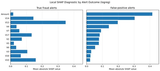
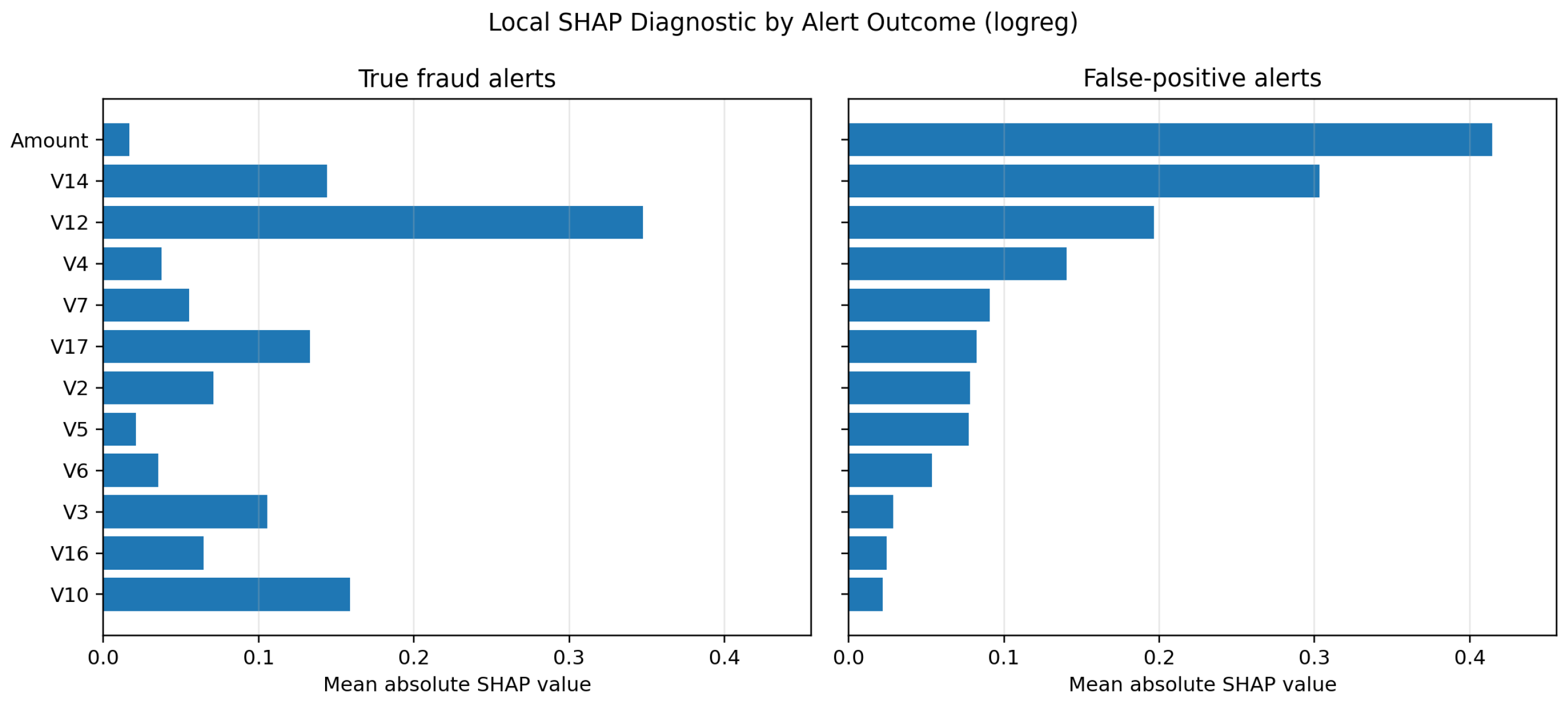
Permutation importance and the 20 local SHAP cases are computational illustrations. Figure 4 uses the LR baseline’s selected true-fraud and false-positive alerts. These observations do not measure human decision quality, explanation actionability or workload.
Figure 4.
Illustrative baseline LR SHAP magnitudes for five selected true-fraud alerts and five selected false-positive alerts. Extreme, outcome-conditioned cases are not a representative analyst evaluation.
5.5. Multiplicity-Controlled Monitoring and No Drift Controls
Table 6 summarises retrospective monitoring. Every temporal chunk triggered Holm-adjusted significance and the D = 0.05 combined alarm for both classifiers. Across monitored variables, maximum KS distance ranged from 0.0985 to 0.1449, while maximum PSI ranged from 0.0470 to 0.1258 and never reached 0.20. The D = 0.10 gate flagged five of six chunks; chunk 2 no longer triggered. Holm correction and effect gating therefore refined interpretation but did not remove the observed marginal shifts.
Table 6.
Fixed-family retrospective monitoring. Values are maxima over the 29 predefined features and the model score. Both classifiers have the same maxima, driven by shared feature distributions.
In 100 empirical iid same-source repetitions per classifier, significance-only alarms occurred in two repetitions (2%), while combined D = 0.05 or PSI alarms occurred in none. A zero count in 100 trials was not proof of zero false-alarm probability; the exact two-sided 95% binomial upper bound was approximately 3.62% under independent control repetitions. The feature resampling was shared across classifiers, so the two zero counts should not be pooled into 200 independent repetitions. Control frequencies described the specified empirical null only. The analysis established neither concept drift nor prospective early-warning lead, and no predictive-degradation lead-time claim is made.
6. Discussion
The completed experiment supports a limited conclusion: acquiring labels can alter ranking performance and review yield, but these outcomes need not coincide with recall improvements or lower hypothetical costs. LR remains the stronger baseline, and its modest AP gains occur with unchanged FN. HGB shows substantial seed variability, and the paired intervals for its selected AP improvements include zero. The full U/R/T policy has no general advantage over simpler scores. These mixed and negative findings are useful when assessing whether a proposed human-feedback component warrants further evaluation.
The simplex analysis tests whether the reference weights are robust across budgets and classifiers. Strong global rank correlations can coexist with different top-budget selections, especially at small budgets. Conversely, distinct weights often select the same cases. Reporting correlations, overlap and distinct-set counts together is more informative than interpreting weights as independent contributions. Selecting the best weight from these held-out comparisons would require a subsequent independent evaluation.
The information-theoretic propositions concern the fitted predictive distribution. Binary entropy expresses ambiguity in bits but adds no independent binary ranking signal. Numerical ties and clipping require explicit treatment when comparing implementations. Entropy mass coverage is a theoretical diagnostic; its empirical concentration is not evaluated in the reported experiment. Label-specific information also differs from information about model parameters or future losses. Uncalibrated probabilities, redundant cases and update dynamics prevent entropy from being equated with learning benefit.
Monitoring detects marginal distribution differences under a specified retrospective family of tests. The fixed feature family avoids future-label-based selection, and the empirical controls show that an effect gate can suppress alarms in a same-source scenario. Neither result establishes production specificity, conditional concept drift or guaranteed advance warning. Production ML additionally requires tested data dependencies, documented update triggers and monitoring governance [23,24,35,40].
6.1. Sensitivity to Cost Assumptions
The cost model is . Coefficients specify hypothetical relative penalties in common units, not salaries, fraud losses or euros. The main setting is a transparent scenario, not an empirically justified business estimate. For paired baseline and acquired-label predictions,
For , the break-even review price is
A negative value rules out a nonnegative break-even review price for that scenario. Table 7 compares the cost scenarios. This calculation omits customer lifetime value, transaction-specific recovery, implementation overhead and delayed investigation outcomes.
Table 7.
Scenario cost comparisons. All coefficients are hypothetical relative penalties. Best acquisition may include tied policies; full ties are exported.
Under the main scenario, P1 is cheaper than every acquisition condition for both classifiers. The cheapest LR acquisition is a tie among U, H and at 0.25%, costing 1546 versus P1’s 1485. Its two-FP reduction offsets ten units, below the 71-unit review charge; break-even is . The cheapest HGB acquisition is random review at 0.25%, costing 1994.8 versus 1918.7. Neither classifier therefore achieves a reduction in mean cost under the main scenario.
At higher FN penalties, HGB at 0.25% has the lowest mean scenario cost: 5116.7 for versus P1’s 5278.7, and 9000.0 for versus 9478.7. These conditional arithmetic comparisons are not demonstrated economic benefits. LR P1 remains cheaper than its acquisition alternatives in all four illustrated scenarios. Across the 144-point coefficient grid, P1 is among the within-family mean-cost minimisers in 114/144 LR settings and 78/144 HGB settings, including ties. Grid frequencies depend on arbitrary scenario spacing and are not probabilities of operational benefit.
6.2. Limitations and Threats to Validity
All empirical conclusions concern a single-dataset, fixed-split, ideal-oracle proof of concept. No independent dataset, real analyst team or prospective deployment was evaluated. Anonymised card data lack merchant, account, device and behavioural context needed to establish present-day e-commerce effectiveness. Thirty seeds describe algorithmic variation; they do not replace independent datasets, and deterministic repetitions do not increase the effective evidence base. Only 22 fraud events occur in the final hold-out, and sparse temporal chunks further limit predictive interpretation.
Single-round acquisition omits label delays, disagreements, noisy analyst feedback, queue capacity over time and adaptive adversaries. The threshold is reselected on a validation window preceding acquired labels, so the comparison is offline. The two classifiers are baselines rather than a comprehensive benchmark of fraud algorithms or imbalance remedies. The weight grid, budgets, cost ratios and drift thresholds are exploratory scenarios. The many comparisons and shared samples preclude confirmatory claims from unadjusted acquisition tests. The empirical no-drift control assumes iid draws from a single observed reference distribution and does not preserve serial dependence.
SHAP and permutation importance describe model behaviour only; explanation usefulness, stability, actionability, actual analyst performance and workload were not measured. Usability, security, trust and maintainability remain conceptual framework attributes, not demonstrated outcomes. No claim of realised cost savings or improved human decisions follows from the experiment.
6.3. Reproducibility and Practical Implications
The Colab notebook and Supplementary Results Document the data hash, software versions, effective estimator parameters, stable ordering, selection rules and per-run outcomes. Re-execution on a different platform can still produce floating-point differences, and the observed U/H exception illustrates why computed priorities and ties deserve explicit attention.
For practical adoption, teams should declare their objective, review capacity, realistic error penalties and monitoring response before selecting an acquisition policy. Independent data, realistic feedback and a controlled analyst study are needed to determine whether any predictive change is useful in operation. The framework identifies those evaluation requirements; the experiment validates only the stated computational components.
7. Conclusions
A completed 30-seed proof of concept compared simulated label acquisition through 12 policies and five budgets, with a 67-setting weight sensitivity analysis and controlled retrospective monitoring. LR’s AP rose from 0.5945 to at most 0.6093 in the reported core settings, while recall remained unchanged and main-scenario cost increased. HGB was substantially seed-sensitive; selected mean AP gains had paired intervals including zero. The composite weights were not generally optimal, and several policies were redundant at larger budgets.
Entropy supplied a diagnostic interpretation of binary ambiguity rather than an independent rank signal. Holm-adjusted, effect-gated monitoring identified marginal temporal shifts, while the same-source control produced no combined alarms in 100 repetitions per classifier; this was limited empirical evidence under the stated null, not a prospective specificity guarantee. Costs and SHAP attributions remained illustrative. Independent and human-centred validation is required before drawing conclusions about operational fraud loss, analyst performance or wider e-commerce deployment.
Supplementary Materials
The following supporting information can be downloaded at https://www.mdpi.com/article/10.3390/e28111211/s1, Table S1: Complete acquisition results; supplementary implementation settings; transaction dataset; raw results and diagnostics; executed and reproduction notebooks; reconstruction and validation scripts; SHA-256 manifests.
Author Contributions
Conceptualization, G.K. and S.K.; methodology, G.K.; validation, A.S.; writing—original draft preparation, S.T. and G.K.; writing—review and editing, S.K. and A.S. All authors have read and agreed to the published version of the manuscript.
Funding
This work was supported in part by the European Union through the Competitiveness Programme (ESPA 2021–2027) under the project easyHPC@eco.plastics.industry (MIS: 6001593).
Institutional Review Board Statement
Not applicable.
Informed Consent Statement
Not applicable.
Data Availability Statement
The dataset is available at https://storage.googleapis.com/download.tensorflow.org/data/creditcard.csv (accessed on 1 October 2026). The completed Colab notebook described in Appendix A is available at https://colab.research.google.com/drive/1w5n6S_78VHo-Xa6gLgZLv-FU7ef--cpt?usp=sharing (accessed on 1 October 2026). The Supplementary Archive supplies raw 30-seed results, weight sensitivity records, monitoring controls, package versions, effective parameters, dataset and output hashes, and scripts that rebuild the manuscript tables.
Acknowledgments
During manuscript revision, ChatGPT 5.6 assisted with language editing and proposed methodological clarifications. The authors retain responsibility for verifying the scientific content, references, code, outputs and interpretations.
Conflicts of Interest
The authors declare no conflicts of interest.
Abbreviations
The following abbreviations are used in this manuscript:
| AI | Artificial Intelligence |
| AUC | Area Under the Curve |
| FN | False Negative |
| FP | False Positive |
| HITL | Human-in-the-Loop |
| ML | Machine Learning |
| PR-AUC | Area Under the Precision–Recall Curve |
| ROC-AUC | Area Under the Receiver Operating Characteristic Curve |
| XAI | Explainable Artificial Intelligence |
Appendix A. Supplementary Implementation Settings
This appendix provides implementation details for the 30-seed experiment. The executable notebook is available at https://colab.research.google.com/drive/1w5n6S_78VHo-Xa6gLgZLv-FU7ef--cpt?usp=sharing (accessed on 1 October 2026).
Appendix A.1. Environment and Data
Recorded versions are Python 3.13.16, NumPy 2.1.3, pandas 2.2.3, SciPy 1.16.3, scikit-learn 1.6.1, Matplotlib 3.10.0, SHAP 0.52.0 and numba 0.61.2. The platform string was Linux-6.6.122+-x86_64-with-glibc2.39. Thread pools were limited to one. The input dataset SHA256 was 76274b691b16a6c49d3f159c883398e03ccd6d1ee12d9d8ee38f4b4b98551a89. Rows were ordered by Time followed by original CSV row ID. Zero-based half-open split ranges were , , and . Predictors excluded Class, source and the original row ID. Thresholds used the linear-interpolated 99th percentile; predictions used greater-than-or-equal comparison. Score priorities were sorted descending with ascending row ID for ties. Random sampling was without replacement, with a fresh default_rng(seed) for each budget and classifier.
Appendix A.2. Estimator and Numerical Settings
StandardScaler used centring, unit variance and copying. Logistic regression used C = 1, balanced classes, primal L2, intercept fitting, lbfgs, max_iter = 1200, tol = and warm_start = false. Histogram boosting used log_loss, learning_rate = 0.06, max_iter = 180, max_leaf_nodes = 31, min_samples_leaf = 20, max_bins = 255, no max_depth, L2 = 0, max_features = 1, class_weight = null, early_stopping = auto, validation_fraction = 0.1, scoring = loss, n_iter_no_change = 10, tol = and warm_start = false. All inputs were numerical; the recorded categorical_features setting was from_dtype. The complete dictionaries preserved remaining effective parameters. The seeds were multiples of 11 from 11 through 330; acquired-label models used seed+1000. Min–max scaling mapped near-constant arrays to zero with NumPy’s default isclose tolerance. Entropy clipped probability at . Permutation importance sampled 6000 future rows with seed 42 and used five repeats. SHAP had 100 training-background rows sampled with seed 20260827, permutation algorithm, seed 20261015 and max_evals = 61. Bootstrap intervals used 20,000 resamples and seed 20260827. The Monte Carlo sign-flip calculation used 100,000 vectors, seed 20261015, absolute signed means, comparison tolerance and the add-one correction. Constant differences produced no test value. Tests were exploratory and unadjusted across acquisition configurations.
Appendix A.3. Monitoring and Sensitivity Files
Monitoring used baseline seed 11, 29 predefined features and scores, six chronological chunks, asymptotic two-sided KS and Holm correction across all 180 comparisons per model. PSI bins used reference deciles, unique edges, infinite endpoints and a proportion floor; degenerate bins used pooled equally spaced edges, and identical constants returned zero. Combined alarms use an adjusted p of at most 0.01 and a D gate of 0.02, 0.05 or 0.10, or PSI of at least 0.20. The empirical control repeated 100 times with replacement from validation; sample sizes matched the temporal analysis, and seed 20261015 was restarted for each classifier. The weight grid contained 67 settings; identical selections shared fits within seed, model and budget. Raw records include selection hashes, Jaccard overlap and distinct-set counts. The cost grid used FN penalties of 20, 50, 100, 200, 500, and 1000; FP penalties of one, five, 10, 20; and review prices of zero, 0.5, one, two, five, and 10. This gave 144 hypothetical combinations. Paired costs and break-even review prices were calculated without refitting.
References
- Thivaios, S.; Kostopoulos, G.; Stefani, A.; Kotsiantis, S. A survey of machine learning and deep learning for financial fraud detection: Architectures, data modalities, and real-world deployment challenges. Algorithms 2026, 19, 354. [Google Scholar] [CrossRef] [Scilit]
- Bolton, R.J.; Hand, D.J. Statistical fraud detection: A review. Stat. Sci. 2002, 17, 235–255. [Google Scholar] [CrossRef] [Scilit]
- Ngai, E.W.T.; Hu, Y.; Wong, Y.H.; Chen, Y.; Sun, X. The application of data mining techniques in financial fraud detection: A classification framework and an academic review of literature. Decis. Support Syst. 2011, 50, 559–569. [Google Scholar] [CrossRef] [Scilit]
- Kotsiantis, S.B. Supervised machine learning: A review of classification techniques. Informatica 2007, 31, 249–268. [Google Scholar]
- Kotsiantis, S.B. Decision trees: A recent overview. Artif. Intell. Rev. 2013, 39, 261–283. [Google Scholar] [CrossRef] [Scilit]
- He, H.; Garcia, E.A. Learning from imbalanced data. IEEE Trans. Knowl. Data Eng. 2009, 21, 1263–1284. [Google Scholar] [CrossRef] [Scilit]
- Chawla, N.V.; Bowyer, K.W.; Hall, L.O.; Kegelmeyer, W.P. SMOTE: Synthetic minority over-sampling technique. J. Artif. Intell. Res. 2002, 16, 321–357. [Google Scholar] [CrossRef] [Scilit]
- Fawcett, T. An introduction to ROC analysis. Pattern Recognit. Lett. 2006, 27, 861–874. [Google Scholar] [CrossRef] [Scilit]
- Davis, J.; Goadrich, M. The relationship between precision-recall and ROC curves. In Proceedings of the 23rd International Conference on Machine Learning, Pittsburgh, PA, USA, 25–29 June 2006; pp. 233–240. [Google Scholar]
- Saito, T.; Rehmsmeier, M. The precision-recall plot is more informative than the ROC plot when evaluating binary classifiers on imbalanced datasets. PLoS ONE 2015, 10, e0118432. [Google Scholar] [CrossRef] [Scilit] [PubMed]
- Breiman, L. Random forests. Mach. Learn. 2001, 45, 5–32. [Google Scholar] [CrossRef] [Scilit]
- Chen, T.; Guestrin, C. XGBoost: A scalable tree boosting system. In Proceedings of the 22nd ACM SIGKDD International Conference on Knowledge Discovery and Data Mining, San Francisco, CA, USA, 13–17 August 2016; pp. 785–794. [Google Scholar]
- Dal Pozzolo, A.; Caelen, O.; Johnson, R.A.; Bontempi, G. Calibrating probability with undersampling for unbalanced classification. In Proceedings of the 2015 IEEE Symposium Series on Computational Intelligence, Cape Town, South Africa, 7–10 December 2015; pp. 159–166. [Google Scholar]
- Dal Pozzolo, A.; Boracchi, G.; Caelen, O.; Alippi, C.; Bontempi, G. Credit card fraud detection: A realistic modeling and a novel learning strategy. IEEE Trans. Neural Netw. Learn. Syst. 2018, 29, 3784–3797. [Google Scholar] [CrossRef] [Scilit] [PubMed]
- Carcillo, F.; Le Borgne, Y.-A.; Caelen, O.; Kessaci, Y.; Oblé, F.; Bontempi, G. Combining unsupervised and supervised learning in credit card fraud detection. Inf. Sci. 2021, 557, 317–331. [Google Scholar] [CrossRef] [Scilit]
- Chen, Y.; Zhao, C.; Xu, Y.; Nie, C.; Zhang, Y. Deep learning in financial fraud detection: Innovations, challenges, and applications. Data Sci. Manag. 2026, 9, 100162. [Google Scholar] [CrossRef] [Scilit]
- Cao, R.; Mao, M.; Wang, X.; Fang, X. Detecting credit card fraud from transaction data streams with incremental time-aware liquid recurrent network. Knowl.-Based Syst. 2026, 331, 114729. [Google Scholar] [CrossRef] [Scilit]
- Zhu, R.; Zhang, X.; Wang, T.; Liao, J.; Chung, S.-H.; Zhang, X. DISCO: Decoupling representation learning and risk control for reliable credit card fraud detection. Decis. Support Syst. 2026, 208, 114717. [Google Scholar] [CrossRef] [Scilit]
- ISO/IEC 25010; Systems and Software Engineering–Systems and Software Quality Requirements and Evaluation (SQuaRE)–System and Software Quality Models. International Organization for Standardization: Geneva, Switzerland, 2011.
- ISO/IEC 25010:2023; Systems and Software Engineering–Systems and Software Quality Requirements and Evaluation (SQuaRE)–Product Quality Model. International Organization for Standardization: Geneva, Switzerland, 2023.
- Stefani, A. Mining metrics for enhancing e-commerce systems user experience. Intell. Inf. Manag. 2022, 14, 25–51. [Google Scholar] [CrossRef]
- Stefani, A.; Vassiliadis, B. ISO25000-related metrics for evaluating the quality of complex information systems. J. Comput. Commun. 2023, 11, 18–43. [Google Scholar] [CrossRef]
- Breck, E.; Cai, S.; Nielsen, E.; Salib, M.; Sculley, D. The ML test score: A rubric for ML production readiness and technical debt reduction. In Proceedings of the 2017 IEEE International Conference on Big Data, Boston, MA, USA, 11–14 December 2017; pp. 1123–1132. [Google Scholar]
- Polyzotis, N.; Roy, S.; Whang, S.E.; Zinkevich, M. Data management challenges in production machine learning. In Proceedings of the 2017 ACM International Conference on Management of Data, Chicago, IL, USA, 14–19 May 2017; pp. 1723–1726. [Google Scholar] [CrossRef] [Scilit]
- Guidotti, R.; Monreale, A.; Ruggieri, S.; Turini, F.; Giannotti, F.; Pedreschi, D. A survey of methods for explaining black box models. ACM Comput. Surv. 2018, 51, 93. [Google Scholar] [CrossRef] [Scilit]
- Doshi-Velez, F.; Kim, B. Towards a rigorous science of interpretable machine learning. arXiv 2017, arXiv:1702.08608. [Google Scholar]
- Ribeiro, M.T.; Singh, S.; Guestrin, C. “Why should I trust you?”: Explaining the predictions of any classifier. In Proceedings of the 22nd ACM SIGKDD International Conference on Knowledge Discovery and Data Mining, San Francisco, CA, USA, 13–17 August 2016; pp. 1135–1144. [Google Scholar]
- Lundberg, S.M.; Lee, S.-I. A unified approach to interpreting model predictions. In Proceedings of the Advances in Neural Information Processing Systems, Long Beach, CA, USA, 4–9 December 2017; Volume 30. [Google Scholar]
- Rudin, C. Stop explaining black box machine learning models for high stakes decisions and use interpretable models instead. Nat. Mach. Intell. 2019, 1, 206–215. [Google Scholar] [CrossRef] [Scilit] [PubMed]
- Sperrle, F.; El-Assady, M.; Guo, G.; Borgo, R.; Chau, D.H.; Endert, A.; Keim, D. A survey of human-centered evaluations in human-centered machine learning. Comput. Graph. Forum 2021, 40, 543–568. [Google Scholar] [CrossRef] [Scilit]
- Wu, X.; Xiao, L.; Sun, Y.; Zhang, J.; Ma, T.; He, L. A survey of human-in-the-loop for machine learning. Future Gener. Comput. Syst. 2022, 135, 364–381. [Google Scholar] [CrossRef] [Scilit]
- Monarch, R.M. Human-in-the-Loop Machine Learning: Active Learning and Annotation for Human-Centered AI; Manning Publications: Shelter Island, NY, USA, 2021. [Google Scholar]
- Settles, B. Active learning literature survey. In Computer Sciences Technical Report 1648; University of Wisconsin–Madison: Madison, WI, USA, 2009. [Google Scholar]
- Amershi, S.; Begel, A.; Bird, C.; DeLine, R.; Gall, H.; Kamar, E.; Nagappan, N.; Nushi, B.; Zimmermann, T. Software engineering for machine learning: A case study. In Proceedings of the 41st International Conference on Software Engineering: Software Engineering in Practice, Montreal, QC, Canada, 25–31 May 2019; pp. 291–300. [Google Scholar]
- Sculley, D.; Holt, G.; Golovin, D.; Davydov, E.; Phillips, T.; Ebner, D.; Chaudhary, V.; Young, M.; Crespo, J.-F.; Dennison, D. Hidden technical debt in machine learning systems. In Proceedings of the Advances in Neural Information Processing Systems, Montreal, QC, Canada, 7–12 December 2015; Volume 28. [Google Scholar]
- Kim, J.; Maathuis, H.; Sent, D. Human-centered evaluation of explainable AI applications: A systematic review. Front. Artif. Intell. 2024, 7, 1456486. [Google Scholar] [CrossRef] [Scilit] [PubMed]
- Vaccaro, M.; Almaatouq, A.; Malone, T. When combinations of humans and AI are useful: A systematic review and meta-analysis. Nat. Hum. Behav. 2024, 8, 2293–2303. [Google Scholar] [CrossRef] [Scilit] [PubMed]
- Shannon, C.E. A mathematical theory of communication. Bell Syst. Tech. J. 1948, 27, 379–423, 623–656. [Google Scholar]
- Cover, T.M.; Thomas, J.A. Elements of Information Theory, 2nd ed.; John Wiley & Sons: Hoboken, NJ, USA, 2006. [Google Scholar]
- Mitchell, M.; Wu, S.; Zaldivar, A.; Barnes, P.; Vasserman, L.; Hutchinson, B.; Spitzer, E.; Raji, I.D.; Gebru, T. Model cards for model reporting. In Proceedings of the Conference on Fairness, Accountability, and Transparency, Atlanta, GA, USA, 29–31 January 2019; pp. 220–229. [Google Scholar]

Disclaimer/Publisher’s Note: The statements, opinions and data contained in all publications are solely those of the individual author(s) and contributor(s) and not of MDPI and/or the editor(s). MDPI and/or the editor(s) disclaim responsibility for any injury to people or property resulting from any ideas, methods, instructions or products referred to in the content. |
© 2026 by the authors. Licensee MDPI, Basel, Switzerland. This article is an open access article distributed under the terms and conditions of the Creative Commons Attribution (CC BY) license.