


Abstract
Accurate process variable forecasting is essential for monitoring, control, and optimization in complex industrial systems. Although existing spatiotemporal forecasting methods have achieved remarkable performance by modeling temporal dependencies and variable interactions, integrating engineering knowledge and data-derived dependencies into both historical encoding and future-target representations remains a modeling challenge. This paper proposes a graph-conditioned forecasting framework for industrial processes. Specifically, a dual-prior temporal–relational encoding aggregation module is developed to integrate an engineering-specified static graph with lagged conditional predictive relationships, enabling unified modeling of physical interactions and causality-informed relationships among process variables. A graph-conditioned query generation mechanism combines future temporal embeddings with variable embeddings augmented by averaged shortest-path-distance embeddings from the data-estimated graph to incorporate structural information into future forecasting queries, while a topology-aware query–state alignment decoder computes an adaptive residual gate to fuse structural priors with historical dynamic states to enhance forecasting representations. In addition, a flow-guided trajectory refinement strategy uses historical process context to refine the initial multivariate forecast trajectories. Compared with the best-performing baseline in each evaluated setting, the framework reduces MSE by approximately 15.4% and 4.9% on the sulfur recovery unit dataset for forecast horizons of 12 and 96 time steps, respectively. On the debutanizer column dataset, the corresponding reductions are approximately 1.9% and 3.0% for horizons of 8 and 12 time steps.
1. Introduction
With the rapid development of Industry 4.0, complex industrial processes are increasingly moving toward digitalized, fine-grained, and intelligent operation [1]. Process variables, which continuously reflect operating conditions, equipment status, and product quality, provide essential information for production scheduling, energy management, and safety assurance. Accurate forecasting of these variables is therefore a fundamental task for industrial artificial intelligence and plays a critical role in improving process reliability and operational efficiency. In a sulfur recovery unit (SRU), for example, anticipating changes in tail-gas and concentrations could help operators assess a developing deviation before a delayed analyzer reading becomes available.
Recent advances in sensor networks and the Industrial Internet of Things have enabled the continuous collection of large-scale multivariate time-series data from industrial plants. Such data contain rich dynamic information, but they also exhibit several characteristics that make forecasting highly challenging. First, industrial processes are governed by complex temporal evolution, where current states are strongly affected by historical operating conditions, delayed responses, and accumulated disturbances. Second, different variables are coupled through physical connections, material flows, energy transfer, and closed-loop control actions. Third, process dynamics may vary across operating regimes because of nonlinear reactions, external disturbances, controller interventions, and load fluctuations. These characteristics motivate the joint use of temporal modeling, inter-variable representations, and available process knowledge [2].
These forecasting requirements have motivated different representations of temporal and inter-variable information. Pathformer divides time series into patches at multiple scales and applies inter-patch and intra-patch attention to represent temporal dependencies [3], while iTransformer represents variables as tokens for attention-based interaction [4]. Graph-based forecasting provides another way to organize sensor relationships, as illustrated by HMTGCN, which combines engineering-informed sensor organization with learned relations for wind-power forecasting [5]. These approaches provide building blocks for learning from multivariate observations, while the source and computational role of industrial process knowledge remain a separate modeling consideration.
In industrial systems, incorporating process knowledge into forecasting connects data-driven models to several overlapping modeling approaches. Physics-informed machine learning is a broad paradigm that incorporates physical knowledge through training objectives, representations, or model design [6]. Physics-informed neural networks (PINNs) are one class of methods within this paradigm. A common formulation combines governing-equation residuals with observation-based losses [7]. Such formulations have also been investigated for systems with incomplete mechanistic descriptions [8]. Gray-box approaches combine prior system knowledge with parameters or model components identified from process data. For example, Schweidtmann et al. describe a broader gray-box category that also includes machine-learning models structured by process knowledge [9]. Closely related hybrid mechanistic and data-driven models explicitly combine mechanistic and learned components. Under the definition adopted by Shah et al., first-principles equations provide the model backbone, while data-driven components represent uncertain parameters or states; these hybrid models are regarded as a subset of gray-box models [10]. Terminology varies across the literature, and broader hybrid AI approaches also incorporate knowledge through tailored representations and architectures [11]. These approaches overlap and differ in how prior knowledge is incorporated, rather than forming mutually exclusive categories. Engineering-specified relationships can provide structural priors without explicitly enforcing governing equations. However, these priors alone do not determine which additional lagged conditional predictive relationships are supported by the observed data. This motivates complementing process knowledge with data-driven identification of such relationships.
Alongside engineering-specified relationships, temporal observations provide another source of relational information. Temporal causal discovery seeks to identify causal relationships from such observations under method-specific assumptions [12], while causality-aware forecasting incorporates causal or causally motivated information into predictive representations [13,14]. In observational industrial records, unmeasured variables, feedback control, and changing operating conditions complicate the interpretation of estimated relations. Temporal precedence or improved prediction alone therefore does not establish intervention-level causality [12]. Engineering knowledge and observation-estimated dependencies can consequently complement one another in forecasting, while retaining distinct sources, assumptions, and evidential meanings.
Despite these advances, integrating process knowledge, data-derived dependencies, and temporal dynamics into industrial forecasting remains challenging. First, attention and token-mixing mechanisms can learn inter-variable dependencies from observations, but such learning does not by itself ensure consistency with engineering-specified relationships. A central challenge is therefore to combine mechanistic structural priors, lagged conditional predictive relationships, and temporal features within a coherent historical representation. Second, future queries constructed from temporal position and variable embeddings do not explicitly encode a target’s position within the process graph. Moreover, although correlation-based graphs can describe statistical associations, their higher-order neighborhoods do not necessarily admit a directed process interpretation. Target representations must therefore incorporate relational structure alongside temporal and variable information. Third, enriching a target representation with relational information does not determine how its forecast depends on the observed process state. This dependence must be modeled through interactions with historical temporal and inter-variable information while preserving target-specific features. Finally, an initial multivariate forecast may retain context-dependent residual errors across its future trajectory. This motivates testing whether the available historical process context can guide a subsequent point-trajectory correction. Together, these challenges motivate a forecasting architecture that integrates historical information, encodes relational target structure, models target–state interactions, and refines multivariate forecast trajectories.
To address these modeling questions, we propose a process-knowledge-guided graph-conditioned forecasting framework. A process-specified graph represents selected engineering relationships and explicitly identified modeling assumptions, while a second graph represents conditional lagged predictive dependencies estimated from training observations. Temporal and relational branches combine these inputs into a historical state. Shortest-path distances in the estimated dependency graph then condition the variable component of future queries, and a gated residual decoder aligns these queries with the historical state. Thus, the supplied process graph influences decoding through the encoded state, while the estimated dependency graph also enters query construction directly. A second-stage flow-matching field, trained with the first-stage predictor frozen, refines trajectories initialized by its forecasts. Engineering knowledge supplies structural guidance, while the numerical prediction and refinement maps are learned from data; the model neither solves governing equations nor guarantees physical feasibility of its outputs. The main contributions of this paper are summarized as follows.
- A dual-prior temporal–relational encoder combines an engineering-specified structure with training-estimated conditional lagged dependencies. Temporal and graph-guided branches are fused into a future-oriented state derived from the historical observations.
- A graph-conditioned decoder query generation mechanism is proposed. By explicitly encoding graph-based structural distance into future forecasting queries, the decoder can construct topology-aware target representations instead of relying only on temporal positions or variable identities.
- A topology-aware query–state alignment decoder is designed to adaptively fuse structural priors and historical dynamic states. The proposed gating mechanism generates dedicated forecasting states for future targets, thereby enhancing the model’s ability to represent complex variable interactions in industrial systems.
- A forecast-initialized flow-matching strategy is proposed to refine the initial multivariate forecast trajectory using graph-conditioned historical context. By freezing the first-stage predictor and learning a separate correction field, the strategy separates relational forecast generation from trajectory refinement.
The remainder of this paper is organized as follows. Section 2 reviews multivariate and graph-based forecasting, physics-informed and hybrid modeling, and temporal causal discovery and causality-aware forecasting. Section 3 defines the forecasting task and relational priors. Section 4 presents the process-knowledge-guided graph-conditioned forecasting framework. Section 5 reports the experiments and analyses. Section 6 concludes the paper and discusses its limitations.
2. Related Work
2.1. Temporal and Inter-Variable Representation for Forecasting
Multivariate forecasting involves representing temporal patterns and interactions among variables. Autoformer and FEDformer combine series decomposition with auto-correlation and frequency-domain modeling, respectively [15,16]. Patch-based Transformers provide another temporal representation: PatchTST uses channel-independent encoding of temporal patches, while Pathformer introduces multiple patch sizes, intra- and inter-patch attention, and adaptive multi-scale pathways [3,17]. Beyond temporal representation, Crossformer models interactions across time segments and variables through two-stage attention, whereas iTransformer treats variates as tokens for attention-based interaction [4,18]. These designs motivate comparisons across different ways of organizing temporal and inter-variable information, while their suitability for an industrial process requires evaluation on its specific data.
Recurrent and state-space models constitute another important line of research for efficient long-horizon forecasting. Instead of relying on quadratic self-attention, SegRNN combines segment-level recurrence with parallel multi-step prediction [19]. In addition, ASTemCN integrates an attention-enhanced LSTM with a causal lower-triangular mask to capture target-series temporal volatility, and employs an attention-based ConvLSTM to trace time-varying topological correlations [20]. Recent Mamba-based models further improve forecasting efficiency through selective state-space modeling. S-Mamba extends the inverted Transformer paradigm to high-dimensional multivariate scenarios by replacing cross-variable self-attention with a lightweight bidirectional Mamba module, enabling near-linear modeling of global variate correlations [21]. Bi-Mamba+ further addresses the tendency of standard Mamba blocks to emphasize local information by introducing a complementary forget gate and a Spearman relation-adaptive decider, which adaptively switches between channel-independent and channel-mixing tokenization according to the strength of data coupling [22].
Convolutional forecasting models exploit local filters, hierarchical receptive fields, and multi-resolution representations to model temporal dynamics. SCINet introduces a tree-structured downsample–convolve–interact architecture, which enlarges the receptive field across multiple temporal resolutions, and an affine interaction mechanism mitigates information loss caused by downsampling and maintains lightweight complexity [23]. TimesNet reformulates one-dimensional time-series modeling as a two-dimensional representation learning problem. By identifying dominant periodicities through the fast Fourier transform and reshaping the sequence accordingly, it enables vision-style backbones to jointly extract intra-period local variations and inter-period long-term evolution patterns [24]. ModernTCN further revisits temporal convolution from a fully convolutional perspective and introduces a decoupled design with large-kernel depth-wise convolution for temporal dependencies and separate convolutional feed-forward modules for feature transformation and cross-variable correlation modeling [25].
MLP- and linear-based models have attracted increasing attention because of their structural simplicity and strong empirical performance. LTSF-Linear demonstrates that a decomposition-enhanced linear architecture can be highly competitive on standard long-term forecasting benchmarks, and provides both channel-independent and channel-mixing variants for multivariate modeling [26]. By sharing time-mixing modules across features and feature-mixing modules among time steps, TSMixer captures temporal patterns and cross-variate correlations with a parameter-efficient formulation [27]. TimeMixer constructs multi-resolution temporal representations through average-pooling-based downsampling, decomposes them into seasonal and trend components, and performs bottom-up and top-down mixing to exchange information across scales [28]. U-Mixer further employs a U-Net-style hierarchical architecture with lateral skip connections to reconcile fine-grained variations and macroscopic trends, and introduces a stationarity correction module to refine prediction trajectories through autocorrelation alignment [29].
In summary, existing LTSF studies have developed diverse temporal representation mechanisms, including attention, recurrence, state-space modeling, convolution, and MLP mixing. Nevertheless, most of them still learn inter-variable dependencies in Euclidean sequence space through implicit token mixing, variable attention, or channel interaction modules. These learned dependencies are flexible and often effective, but they are not explicitly constrained to follow the physical connections, causal directions, or control pathways that govern industrial processes.
2.2. Graph-Based Spatiotemporal Forecasting
In multivariate time-series scenarios such as traffic flow, weather forecasting, and wind power prediction, exploiting non-Euclidean topological relations among variables has become an effective strategy for improving forecasting performance. The central challenge is to jointly characterize spatial dependencies, which may be local or global, and temporal dynamics, which are often nonlinear and time-varying. Graph neural networks (GNNs) address this issue by updating node representations through topology-guided information propagation. According to the design of graph filters and message-passing operators, existing spatiotemporal forecasting methods can be broadly grouped into spectral GNNs, spatial GNNs, and hybrid graph models, which are commonly coupled with RNNs, CNNs, or attention mechanisms for temporal modeling.
Early graph-based time-series forecasting methods represent sensors as graph nodes and employ graph convolution over predefined topologies to capture spatial dependencies, while temporal dynamics are represented by temporal convolution [30] or attention mechanisms [31]. ST-MGCN enriches spatial semantics by introducing multiple heterogeneous graphs, including spatial proximity, functional similarity, and transportation connectivity, into a unified graph convolutional framework [32]. Later studies relax the dependence on manually defined topology by learning adaptive adjacency matrices from node embeddings, allowing latent spatial correlations to be captured beyond physical connectivity [33,34]. DGCRN further constructs step-wise dynamic graphs from current traffic states, temporal features, and recurrent hidden states through a hyper-network, and fuses the resulting dynamic graph with a predefined static road graph inside graph-convolutional recurrent units [35].
Beyond these representative architectures, subsequent studies can be roughly discussed from the perspectives of spectral graph modeling and spatial message-passing design. Spectral graph models enhance relation modeling by constructing graph filters or structural encodings in the graph frequency domain. MSGNN employs a magnetic signed Laplacian to represent positive and negative correlations as well as directed topology, encoding edge directions into complex phases and relation signs into Hermitian matrices [36]. Temporal Graph Gegenbauer Convolution (TGGC) constructs graph spectral filters using orthogonal Gegenbauer polynomials, enabling the model to fit heterogeneous graph signal densities and capture multi-scale spatial correlations [37]. STWave+ can be regarded as a hybrid spectral–spatial model because it combines localized graph attention over predefined physical layouts with structural positional embeddings derived from Laplacian eigenvectors, thereby balancing spectral priors and data-driven spatial flexibility while reducing the complexity of dense graph attention [38].
Spatial and hybrid graph models, in contrast, mainly construct neighborhoods or relation weights in the node domain and then perform message passing or attention-based aggregation. TSGAN uses dynamic time warping to quantify temporal-pattern similarity among cellular traffic nodes and constructs a sparse graph for graph attention-based forecasting [39]. TFSGFTN integrates Transformer-based sequence encoding, Fourier-domain modulation, and graph attention over a fully connected sensor graph for aeroengine health indicator prediction [40]. HMTGCN combines adaptive graph learning to capture fine-grained variable interdependencies within sensor clusters with coarse-grained graph convolution over engineering-prior topologies, providing a practical strategy when only limited physical knowledge is available [5]. SDGFNet fuses a prior static graph with input-dependent multi-scale dynamic graphs learned from wavelet-decomposed sequences, and employs attention-gated fusion to balance stable and evolving correlations [41]. STDN jointly learns dynamic node relationships, graph-Laplacian-based spatial embeddings, and temporal periodic embeddings, and then models the resulting representations through a GRU encoder and Transformer decoder [42]. Not all spatiotemporal forecasting models rely on explicit graph neural networks. M3-Net replaces road-network graph construction and message passing with node and time embeddings, adaptive spatial grouping, and channel-wise mixture-of-experts learning, thereby achieving graph-free spatiotemporal representation for traffic prediction [43].
These representative methods demonstrate the effectiveness of graph-based spatiotemporal modeling, but their learned relations are often correlation-oriented and may not directly correspond to physical mechanisms or causal effects.
2.3. Knowledge-Guided Process Modeling
Physics-informed machine learning has been implemented through relational representations as well as equation-based objectives. Liu et al. [44] construct a conditional Granger causality graph from training data and combine graph-based information with sparsity-regularized, sample-specific information in a two-stream soft sensor for penicillin fermentation. This approach incorporates relational guidance without imposing governing-equation residuals in the loss. However, a data-derived predictive-dependence graph should be distinguished from engineering-specified physical relationships. When partial governing equations are available, Velioglu et al. develop PINNs for dynamic processes with incomplete semi-explicit differential–algebraic models, combining observation and initial-condition errors with residuals of the available equations [8]. For linear chromatographic models, Chen et al. [45] incorporate order-of-magnitude analysis into the PINN loss to account for disparate scales in the modeled dynamics. Hybrid and gray-box models, whose terminology overlaps in the literature, retain mechanistic calculations while using data-driven components to supplement selected parts of the model. Kay et al. [46] augment Langmuir–Hinshelwood and power-law kinetic models with a neural network for water–gas shift and methanol synthesis. Wen et al. [47] combine Gaussian-process regression with a heat-balance model to predict conversion, temperature, and heat flow in sulfuric-acid-catalyzed esterification. At the flowsheet level, Winz et al. [48] replace computationally expensive submodels with surrogates while retaining the surrounding process equations, and propagate uncertainty through sensitivity analysis for Bayesian optimization. These approaches motivate distinguishing structural guidance from equation-based constraints and retained mechanistic calculations when incorporating process knowledge into forecasting.
2.4. Causality-Aware Prediction
Causality-aware forecasting incorporates estimated temporal and inter-variable dependencies into predictive models. Causal-TSF [49] combines hidden-confounder estimation with sampling-based debiasing to mitigate confounding effects in time series forecasting. ARCausal [50] combines transfer-entropy-based dependency analysis with vector-autoregressive estimation to construct a sparse causal mask for Transformer attention. These approaches incorporate causal information through confounder adjustment or dependency-guided attention masking. DANCE [51] combines delay estimation, consensus causal-structure exploration, and causality-aware attention for virtual sensing in a debutanizer process, highlighting the importance of accounting for delayed dependencies in industrial process modeling. Diff-MGR [14] combines dynamic causal graph attention and pattern reproduction with conditional diffusion for multivariate probabilistic forecasting.
2.5. Method Positioning and Scope
The reviewed approaches differ in where and how temporal information, variable relationships, and process knowledge enter prediction. The temporal forecasting models considered above learn variable interactions without an engineering-specified graph, while graph-based and causality-aware methods introduce relational information through different representation and prediction mechanisms. Knowledge-guided process models further incorporate engineering structure or mechanistic formulations. Within these reviewed designs, the coordinated use of engineering-specified relations and training-estimated lagged dependencies across historical encoding and future-target modeling remains a relevant modeling issue for industrial forecasting.
The proposed framework is positioned as knowledge-guided, data-driven forecasting, with relational structure informing both historical and future representations and historical context supporting subsequent trajectory refinement. Table 1 summarizes this positioning relative to the reviewed technical approaches.
Table 1.
Positioning of the proposed framework relative to representative modeling approaches reviewed in this section.
3. Problem Formulation
3.1. Multivariable Time Series Forecasting
Consider an industrial process monitored by C process variables. At time step t, the multivariate observation is denoted as . Given a historical window with look-back length L, the input sequence is defined as The objective of multivariate time-series forecasting is to estimate the future trajectory over a horizon of H.
Let denote an adjacency matrix that characterizes the spatial or relational dependency among process variables. The graph structure can be specified by prior process knowledge, derived from engineering rules, inferred from data, or obtained by combining multiple information sources. The graph-enhanced forecasting problem can then be formulated as
where is a forecasting model parameterized by , and is the forecast sequence. The model is trained by minimizing the discrepancy between the forecast and the ground truth:
where denotes a point-wise forecasting loss, such as the squared error or absolute error.
3.2. Graph Representations in Industrial Systems
Industrial systems involve heterogeneous dependencies among process variables. A single graph is usually insufficient to describe both stable mechanism-supported relations and operating-condition-dependent dynamic relations. In this work, two complementary graph representations are considered: a static mechanism graph and a causality-informed lagged relation graph . These graphs are constructed before forecasting-model training and are treated as external structural inputs rather than learned components of the proposed architecture.
The forecasting framework is agnostic to the specific procedure used to construct the causality-informed relation graph. When reliable process knowledge or an externally validated causal graph is available, the corresponding adjacency matrix can be supplied directly. Otherwise, the graph can be estimated from training observations using an existing conditional-dependence method, such as Gaussian conditional mutual information (CMI) or conditional Granger causality. In all cases, the graph is constructed independently of the forecasting model and is treated as an external structural prior.
3.2.1. Static Mechanism Graph Construction
The static mechanism graph is denoted by , where is the set of process variables, is the set of mechanism-related edges, and is its adjacency matrix. In industrial processes, can be constructed from piping and instrumentation diagrams, process flow diagrams, control-loop configurations, or expert knowledge. The static adjacency is defined as
3.2.2. Causality-Informed Relation Graph
Although the static mechanism graph provides interpretable prior knowledge, it is time-invariant and may not fully capture dynamic dependencies induced by changing operating conditions, disturbances, and delayed responses. To complement this limitation, a causality-informed relation graph is introduced and represents directed relationships inferred from historical process data over a specified time interval. Compared with pairwise correlation, causal analysis aims to identify directional influence among variables. In multivariate industrial systems, conditional directed dependence is particularly important because the dependency between two variables may be confounded or mediated by other process variables.
The causality-informed graph characterizes lagged conditional predictive relationships, namely whether the past of a candidate source variable provides additional information for predicting the current value of a target variable after accounting for the histories of the remaining observed variables. Let denote the p-lag history of candidate source , and let collect the corresponding lagged histories of all variables other than . Because , the conditioning set includes the history of target . For each ordered pair , the lagged conditional-dependence strength is defined generically as
where denotes a conditional directed-dependence estimator. The direction is induced by temporal ordering: the history of is used to explain the current value of . A larger indicates that the source history provides more information about the current target beyond that contained in the remaining observed histories. In this work, conditional Granger causality and Gaussian conditional mutual information are considered as two alternative estimators of this quantity.
For conditional Granger causality, a full ridge autoregression containing the lagged histories of all variables is compared with a restricted model in which all lagged terms of candidate source are removed. The score is
where and are the residual sums of squares of the restricted and full models, respectively. A positive score indicates that including the source history reduces the target regression error after conditioning on the other observed histories.
Alternatively, Gaussian conditional mutual information measures the conditional dependence between the source history and the current target. Its score is defined as
where , , and . Here, , , and denote the covariance matrices of the corresponding concatenated variables.
The causal interpretation of the graph relies on several assumptions. First, the data-generating process is assumed to be approximately stationary over the training interval. Second, the procedure focuses on lagged relationships and does not identify contemporaneous effects occurring within the same sampling interval. Third, the maximum lag p is assumed to cover the relevant dependency horizon at the adopted sampling frequency. Accordingly, the discovered edges should be interpreted as conditional lagged predictive, or Granger-causal, relationships rather than intervention-based causal effects. Based on the conditional Granger score and Gaussian conditional mutual information defined above, we construct a directed lagged conditional-dependence graph using Algorithm 1. The estimator is instantiated using either the conditional Granger estimator or the Gaussian conditional mutual-information estimator described in Equations (5) and (6), respectively. Nevertheless, Algorithm 1 can accommodate another conditional-dependence estimator as long as it produces a nonnegative score whose magnitude represents the strength of the conditional lagged relationship.
| Algorithm 1 Training-based construction of a lagged conditional-dependence graph |
|
The static mechanism graph and the dynamic causality-informed graph provide complementary relational priors. The former encodes stable physical and control-related knowledge, whereas the latter captures data-driven directional dependencies that may vary with operating conditions. The forecasting problem studied in this paper is therefore formulated as
3.3. Patch-Based Representation
To improve long-horizon modeling efficiency and preserve local temporal evolution, the original multivariate time series is transformed into a patch-based representation before being fed into the forecasting model. The historical sequence is divided into non-overlapping temporal patches:
The patch-based input tensor is then written as Similarly, the future sequence is represented as M target patches Let denote the patching operator with patch length S and the historical input and future target sequences are represented as patch tensors:
Based on this representation, the sequence-level forecasting model in (7) is implemented through a patch-level forecasting module:
where denotes the patch-level forecasting function and denotes the forecast future patches. The sequence-level forecast is recovered using the inverse reshaping operator , which restores the temporal sequence from the predicted patches:
4. Methodology
4.1. Framework Overview
As shown in Figure 1, the overall framework consists of four coupled components. First, a dual-prior temporal–relational encoder combines learned temporal features with an engineering-specified static graph and a graph of lagged conditional predictive relationships estimated from training observations before predictor training. These graphs provide structural guidance for relational aggregation without imposing first-principles differential equations as explicit constraints. Second, graph-conditioned future queries combine future temporal embeddings with variable embeddings augmented by dependency-graph distance information. Third, a topology-aware query–state alignment decoder calibrates these future target coordinates with historical representations to form target-specific forecasting states. The encoder projections, lag and fusion weights, query embeddings, decoder gates, and prediction head are learned during first-stage training. Finally, a flow-matching-based second-stage strategy learns a transport field from the forecasting prior to the target distribution, providing trajectory-level refinement without discarding the structural forecasting capability learned in the first stage. Table 2 summarizes the origin of the graph specification or learned parameters and learning procedures of the framework components, together with their design reuse and adaptation requirements for a new process.
Figure 1.
Overall architecture of the proposed mechanism-informed causality-aware spatiotemporal forecasting framework. Yellow and green arrows indicate the construction pathways for the static mechanism graph and the data-driven causal relation graph, respectively; gray arrows indicate information flow between modules.
Table 2.
Component sources, learning procedures, and requirements for reuse across processes.
4.2. Dual-Prior Temporal–Relational Encoding
Industrial process variables are coupled by heterogeneous relations. Some dependencies are stable because they are induced by material transfer, equipment connectivity, reaction constraints, or control loops; others are expressed as delayed conditional influence in historical observations. Treating these two sources as a single learned adjacency may obscure their different physical meanings and make the learned representation sensitive to noise or operating-regime variation. We therefore use a dual-prior representation to separate engineering-specified structural guidance from data-inferred lagged causality.
Let denote the encoded historical patch representation, where B is the batch size, N is the number of input patches, C is the number of variables, and D is the hidden dimension. The element represents the hidden state of variable in the n-th historical patch of the b-th sample.
4.2.1. Mechanism-Informed Static Graph
The static mechanism graph is specified using the process-knowledge categories summarized in Table 3. These mechanism-supported relations define the nonzero entries of and provide an interpretable prior topology for graph-guided forecasting.
Table 3.
Process-knowledge categories used to specify the static mechanism graph.
Let denote the static adjacency matrix, where represents the strength of the directed relation from source variable i to target variable j. To encode stable mechanism-supported interactions, static graph message passing aggregates information from the physical predecessors of each target variable:
where is a learnable projection matrix. If the j-th row of contains no incoming mechanism-supported edges, then for all i. This operation propagates information along mechanism-supported paths such as material transfer, feedforward control, feedback regulation, and reaction-related constraints. The static branch is then projected to the future patch horizon:
where is a learnable projection along the patch dimension.
4.2.2. Causality-Informed Temporal Relation Graph
To model lagged conditional predictive dependencies that may not be captured by instantaneous structural propagation, lagged causal message passing aggregates causal predecessors from previous patches. Given a maximum lag order K, the lag weights and lagged causal message are defined as
where are learnable lag logits, is a learnable projection matrix, and is set to zero when . The target variable therefore aggregates lagged messages from its causal source variables according to the causality-informed lagged relation graph. The lagged causal branch is also projected to the future patch horizon:
where is a learnable projection along the patch dimension. This design reflects the fact that causal effects in industrial processes are often delayed rather than instantaneous.
4.2.3. Temporal Attention
To capture temporal evolution along the patch dimension without mixing variables, the temporal branch extracts temporal dependencies by applying self-attention along the patch dimension for each variable. For variable , the query , key , and value matrices are constructed from its historical patch states:
where , , and are learnable projections. The temporal attention output is
In industrial chemical processes, the influence of historical information on future system dynamics generally decays with increasing temporal distance. Therefore, the latest attended temporal state is selected and expanded to the future horizon:
where is the last token of .
To provide the decoder with both historical dynamic information and graph-guided relational context for all future patches, the final graph-guided state is obtained by fusing temporal, static mechanism, and lagged causal branches:
where , , and are learnable branch coefficients. The resulting tensor , as a future-oriented historical state, preserves temporal dynamics from observed patches while embedding the mechanism and causal pathways through which industrial variables influence one another.
4.3. Graph-Conditioned Query Generation
In conventional sequence decoders, future queries are usually constructed from temporal positional embeddings or variable embeddings. Such queries specify when and which variable to predict, but they leave the future target structurally under-specified, which means that two variables with very different positions in the process topology may still be decoded from similarly formed tokens. To explicitly encode how variables are structurally related, a graph-conditioned decoder query is constructed by injecting graph-distance information into the variable query embedding, so that each future target is represented as a topology-aware latent coordinate before interacting with historical states.
Let denote the shortest-path distance from to on , which provides a compact description of how a variable is positioned relative to other variables. For each target , the three largest off-diagonal entries in row j are retained, while all other entries are discarded. Each retained edge is treated as having unit length, irrespective of its original weight. Self-distances are set to zero. Distances greater than or equal to , including unreachable pairs, are mapped to the shared index . For variable , its graph-distance context is defined as
where is a learnable distance embedding representation.
Let denote the learnable temporal embedding for future patches, and let denote the learnable variable embedding. The graph-conditioned variable embedding is then obtained by
where is a learnable scalar gate. This formulation keeps the original variable identity while adding a topology-dependent correction derived from graph distances. Finally, the decoder query for future patch m and variable is constructed as
Through this construction, the forecasting query is no longer determined only by temporal position and variable identity. It also carries structural information about the graph neighborhood and relative position of each variable in the industrial process topology.
4.4. Topology-Aware Query–State Alignment Decoder
The graph-conditioned query defines the structural coordinate of a future forecast target, while the encoded state provides process-dependent dynamic information extracted from historical observations. The future target coordinate must be calibrated by the historical state so that the final latent state reflects both where the variable is located in the process topology and how the process has evolved before the forecasting point. Therefore, a topology-aware query–state alignment decoder is introduced. For notational simplicity, the batch index b is omitted in the decoder equations.
The query and state representations are first projected into a shared alignment space:
where and are learnable projection matrices. An adaptive alignment coefficient is then computed as
where controls the element-wise alignment strength between the topology-aware future query and the encoded historical state. The encoded state is mapped into the forecasting-state space:
where is a learnable projection matrix.
The final forecasting state is obtained by residual query–state alignment:
where ⊙ denotes element-wise multiplication. The initial query preserves the structural identity of the future targets, whereas acts as a state-dependent reference derived from the observed trajectory. The coefficient specifies how far each latent dimension should move from the structural coordinate toward the historical reference. As a result, the decoder synthesizes a target-specific forecasting state by calibrating topology-aware future queries, rather than relying on generic positional queries or recurrent state transitions. The future patch value is finally generated by a prediction head:
where denotes the predicted segment of variable in the m-th future patch.
4.5. Flow-Guided Trajectory Refinement
Although the graph-conditioned forecasting module captures the dominant temporal–relational evolution, industrial trajectories remain affected by stochastic disturbances, unobserved operating variations, and nonlinear transient responses. A single-stage deterministic objective may force the same model parameters to learn both structural forecasting and distributional refinement, which can increase training variance across runs. To separate structural forecasting from subsequent trajectory correction, we introduce a forecast-initialized flow matching strategy with two training stages.
The first stage learns a structural forecasting model using the supervised objective in Equation (2). In the second stage, the trained patch-level forecasting module is kept fixed, and the initial source trajectory is provided by
where is the patch-level forecasting function with the parameters learned in the first stage. Unlike conventional generative flow matching, which usually transports samples from a simple noise distribution to the data distribution, the proposed formulation takes the deterministic first-stage forecast as the source state, and the second stage learns a conditional trajectory transport field that moves the source forecast toward the target trajectory for correcting its residual trajectory errors.
For each training pair , we construct a linear interpolation path and sample an interpolation time uniformly from :
where is the complete intermediate trajectory state, and parameterizes the transition between the source and target trajectories. Differentiating the interpolation path with respect to gives the target transport velocity
The conditional velocity field predicts a transport velocity, where denotes the learnable field parameters and is the graph-conditioned historical context produced by the forecasting backbone. The field is trained using the flow-matching loss
where denotes the empirical distribution of training input–target pairs, is the uniform distribution, and denotes the Euclidean norm after vectorizing the patch tensor. The source forecast remains fixed while the objective encourages the field to learn both the direction and magnitude of the correction across the future sequence.
During inference, the source forecast and historical context are obtained from the observed input. The learned field then defines an evolution of the forecast state :
This differential equation specifies the inference dynamics driven by the learned velocity field. The inference path is generated by integrating the field from the source forecast, approximated using R explicit updates with step size . Let denote the numerical state after r updates, initialized as . Following the midpoint time schedule , the update is
At each step, the velocity is recomputed from the current numerical state and the selected interpolation time. Accumulating these updates gives
During inference, the velocity field trained on the interpolation paths is integrated from the source forecast to generate the refinement trajectory. The final forecast is obtained by scaling the accumulated displacement from the source forecast:
where is the refined future patch tensor and controls the bounded refinement strength of the correction through .
5. Experiments
This section reports the experimental evaluation on a publicly available industrial sulfur recovery unit benchmark (SRU) dataset [52] and the debutanizer column (DC) dataset [53]. The experiments include comparison with representative forecasting baselines, component analysis, robustness evaluation, sensitivity analysis, and computational efficiency analysis.
5.1. Experimental Setup
The SRU dataset contains 7 time series variables, which include MEA gas flow, primary air, secondary air, SWS air, SWS gas, and tail-gas concentrations of and . These variables cover both manipulated operating variables and product-quality indicators, and are coupled through combustion, catalytic conversion, material transfer, and feedback control. The DC dataset contains seven routinely measured process variables and the bottom-product butane-content indicator. The variables describe top temperature and pressure, reflux flow, flow to the downstream process, sixth-tray temperature, and two bottom-temperature measurements.
An SRU forecast can help an operator assess how changes in gas feed and combustion-air flow may be followed by deviations in tail-gas composition. In a debutanizer column, anticipating changes in bottom-product butane content can similarly support the assessment of developing product-quality deviations. These examples motivate forecasting as a source of information for monitoring and operational decisions, which is formulated as a multivariate multi-step forecasting problem, and future process states are estimated from historical observations. The descriptive statistics are reported in Table 4.
Table 4.
Variable definitions and descriptive statistics on the released scales. IQR denotes the interquartile range.
Let L and H denote the lengths of the input window and forecast horizon, respectively. To evaluate model performance across different temporal scales, two representative forecasting configurations for each dataset are adopted, corresponding to short-horizon and long-horizon forecasting scenarios, as shown in Table 5. Neither public dataset provides explicit operating-regime labels; therefore, regime-specific forecasting performance was not separately assessed. Before splitting the dataset, data-integrity checks found no missing or non-finite values or duplicate rows in either dataset. No automated outlier detection or treatment was applied, and all observations were retained, as abrupt changes and extreme values may reflect physically meaningful process transients. The dataset is split in chronological order into training, validation, and test subsets with a ratio of 6:2:2. Within each split, stride-one sliding windows were constructed, giving training windows. To avoid information leakage, all data-dependent preprocessing steps are fitted exclusively on the training subset. Specifically, feature-wise z-score standardization is performed using StandardScaler, with the training-set means and standard deviations applied to the training, validation, and test subsets. The causality-informed graph is also inferred exclusively from the training subset. Unless otherwise specified, all competing methods use the same data partitions, preprocessing procedure, and forecasting protocols. Results are reported as the mean ± standard deviation over five independent runs.
Table 5.
Dataset characteristics and forecasting tasks. Split sizes count original time points before windowing. Training-window counts do not represent independent observations.
5.2. Baselines, Metrics, and Tuning
The compared methods include representative Transformer-based, patch-based, MLP-based, RNN-based, CNN-based, graph-based, and causality-aware forecasting models: Transformer, Informer, Autoformer, FEDformer, Crossformer, PatchTST, iTransformer, LightTS, MSGNet, NST-Transformer, SegRNN, Mamba, S_Mamba, TimesNet, ModernTCN, TimeMixer, TSMixer, WPMixer, DLinear, FreTS, MTGNN, GraphWaveNet, AGCRN, StemGNN, STDN, STWave, ARCausal, and Causal-TSF. To ensure fair comparisons, hyperparameters that were shared by the proposed model and the competing methods were optimized using the same two-stage procedure. Architectural hyperparameters were first selected through grid search, followed by Optuna-based optimization of the remaining applicable hyperparameters. Baseline-specific hyperparameters without direct counterparts in the proposed model were fixed to the recommended settings provided in their official implementations. Parameters were searched only when the corresponding components were present. The shared search dimensions and ranges are summarized in Table 6. Where patching was required, the input and target sequences were zero-padded to form complete patches, and the padded target positions were excluded from both loss computation and evaluation.
Table 6.
Hyperparameter search space and selected configurations of the proposed two-stage model. “Fixed” denotes a parameter that was not included in hyperparameter search. For the DC dataset, the hidden dimensions 128/256 correspond to input–forecast length pairs and , respectively. All other configurations are shared across the two forecasting tasks within each dataset.
Hyperparameter tuning began with an exhaustive grid search over the hidden dimension and number of attention heads, evaluating 12 candidate configurations. After fixing the selected architectural settings, Optuna was used to tune the dropout rate, patch length, learning rate, causal graph lag, maximum graph distance, and refinement scaling parameter. The Optuna search employed the tree-structured Parzen estimator and was limited to 50 trials per forecasting task.
For all methods, each candidate configuration was evaluated over five independent training runs, and selection was based on the mean validation MSE using the same chronological data split. Each run was trained for at most 100 epochs, with early stopping when the validation MSE did not improve for 30 consecutive epochs. The checkpoint with the lowest validation MSE within each run was retained. All experiments were collected under the same hardware environment and batch setting. The hardware configuration is summarized in Table 7.
Table 7.
Hardware configuration for runtime evaluation.
To comprehensively assess the accuracy and alignment of the predictive models, three widely adopted evaluation metrics are employed: Mean Squared Error (MSE), Mean Absolute Error (MAE), and Dynamic Time Warping (DTW) distance. MSE and MAE measure point-wise forecasting accuracy, whereas DTW evaluates trajectory-shape alignment under possible phase shifts or delayed responses. Let denote the ground-truth and forecast sequences. The metrics are defined as
where and denote the entries of and , respectively; flattens an array row by row, and W is a valid warping path between the resulting sequences.
Results are reported as mean ± standard deviation across independent runs. In the main comparison tables, MSE and MAE statistics are rounded to two decimal places, with nonzero values below 0.005 expressed in scientific notation with one significant figure. DTW means are rounded to one decimal place, while DTW standard deviations are rounded to one decimal place for values and to two decimal places otherwise. In the ablation tables, MSE and MAE values are reported to three decimal places to preserve small differences among variants, while DTW values and relative percentage changes are reported to one decimal place.
5.3. Process-Specific Relational Priors
5.3.1. Engineering-Graph Specification
The static mechanism graph is constructed as a selective representation of process knowledge among the available variables, where denotes an engineering-specified relationship from to . Edges are specified when a process-relevant relationship can be supported by the flowsheets, equipment descriptions, control logic, or physicochemical principles. The graph is not intended to exhaustively enumerate all physical dependencies and an omitted edge therefore does not imply the absence of a physical relationship. Figure 2 shows the engineering-specified static graph prior weights for the SRU and DC datasets. The corresponding dependency mechanisms are listed in Table 8 and Table 9, respectively.
Figure 2.
Engineering-specified static graph prior weights: (a) the sulfur recovery unit (SRU) and (b) the debutanizer column (DC).
Table 8.
Sources and process rationale for the engineering-specified SRU graph. Relation types are defined in Table 3.
Table 9.
Sources and process rationale for the engineering-specified DC graph. Relation types are defined in Table 3.
5.3.2. Causality-Informed Graph Specification
We constructed lagged conditional-dependence graphs for both the SRU and DC datasets following Algorithm 1. The SRU dataset contains seven process variables, whereas the debutanizer dataset contains eight variables. For each dataset, graph estimation was performed using only the chronologically ordered training partition. The variable-wise means and standard deviations were calculated from this partition and used to standardize the graph-estimation samples. Figure 3 presents the row-normalized graph weights estimated using Gaussian conditional mutual information with a maximum lag order of . Gaussian CMI uses sample covariance matrices regularized by adding before log-determinant evaluation.
Figure 3.
Lagged conditional-dependence graph weights: (a) the sulfur recovery unit (SRU) and (b) the debutanizer column (DC).
5.4. Comparison Results
The forecasting comparison covers two configurations for each of the SRU and DC datasets. The proposed model achieves the lowest mean MSE and DTW in all four tasks, together with the lowest mean MAE in three tasks and a tie at the reported precision in the remaining task. In addition, the lower variance suggests that the flow-guided refinement stage constrains the learning process toward more reproducible solutions, rather than relying on run-dependent latent correlations.
For the SRU dataset, Table 10 and Table 11 report results for and , respectively. The proposed model achieves the lowest errors across all three metrics in both configurations. Its MSE values of 0.22 and 0.58 correspond to approximate reductions of 15.4% and 4.9% relative to the best baseline MSEs of 0.26 and 0.61, respectively. The relative MSE improvement is therefore larger for the shorter-horizon configuration, while the longer-horizon configuration retains an advantage across all three metrics.
Table 10.
Forecasting performance comparison on the SRU dataset using a forecasting horizon of 12 with an input length of 48. The best result is bold and the second-best result is underlined.
Table 11.
Forecasting performance comparison on the SRU dataset using a forecasting horizon of 96 with an input length of 336. The best result is bold and the second-best result is underline.
For the DC dataset, Table 12 and Table 13 report results for and , respectively. The proposed model obtains MSE values of 0.51 and 0.64, improving on the best baseline values of 0.52 from MTGNN and 0.66 from SegRNN by approximately 1.9% and 3.0%, respectively. It also achieves the lowest mean DTW in both configurations. For MAE, it ties with SegRNN at 0.46 in the configuration at the reported precision and achieves the lowest value of 0.53 in the configuration. Thus, the improvements extend to DC, although the relative MSE gains are smaller than those observed on SRU.
Table 12.
Forecasting performance comparison on the DC dataset using a forecasting horizon of 8 with an input length of 12. Results are reported as mean ± standard deviation. The best result is bold and the second-best result is underlined.
Table 13.
Forecasting performance comparison on the DC dataset using a forecasting horizon of 12 with an input length of 48. Results are reported as mean ± standard deviation. The best result is bold and the second-best result is underlined.
Figure 4 provides a qualitative comparison of the forecast trajectories. For the operating variables, all competitive models can capture the dominant steady-state levels, but visible deviations appear around abrupt step changes and transient peaks. The proposed model follows the sharp transitions of more closely than the less stable trajectories, and it avoids the pronounced overshoot observed for some baselines around large operating shifts in . For the two tail-gas quality variables ( and ), the forecasting task is more challenging because the trajectories contain intermittent spikes and abrupt changes. The proposed forecast remains close to the operating band for most time indices and tracks several local excursions without producing persistent bias.
Figure 4.
Forecasting performance for selected variables in the SRU 48-to-12 multivariate forecasting task. All variables are shown on the standardized scale (z-scores). The red shading indicates the 20th–80th percentile range of the proposed model’s overlapping forecasts at each sample position. (a) . (b) . (c) . (d) .
5.5. Uncertainty Analysis Under Temporal Dependence
5.5.1. Window Overlap and Temporal Dependence
Under the 60%/20%/20% split used in the final experiments, the SRU and DC training partitions contain 6048 and 1436 time observations, respectively. The corresponding numbers of stride-one training windows depend on the input and prediction lengths, as reported in Table 5. However, the nominal window counts substantially overstate the number of independent samples: neighboring windows are largely shifted views of the same process trajectory. This dependence motivates an uncertainty analysis that accounts for the temporal structure of the evaluation errors.
The proposed model is compared with the strongest non-proposed baseline on SRU with and DC with . Forecast origins are spaced one prediction horizon apart, yielding 17 and 35 evaluation origins, respectively, with non-overlapping target intervals. Using a paired circular block bootstrap with a block length of 8 and 2000 resamples, the same origin blocks are resampled for both models, preserving their matched evaluation and the local temporal structure of the errors.
Figure 5 reports the resulting MSE distributions and paired differences, defined as . The proposed model achieves a lower mean MSE on both tasks under horizon-separated evaluation. The paired distributions are centered below zero, and their 95% block-bootstrap intervals exclude zero with the specified block length of 8. These results support an advantage over the selected baseline on both tasks under this dependence-aware evaluation procedure. The stride-one results are therefore interpreted as descriptive benchmark estimates, while the paired block-bootstrap analysis assesses uncertainty in the model differences.
Figure 5.
Dependence-aware uncertainty analysis for the SRU 336–96 and DC 48–12 forecasting tasks. (a) Circular block-bootstrap distributions of the absolute MSE for SegRNN and the proposed method. (b) Distributions of the paired MSE difference, defined as . White circles denote point estimates, and vertical error bars denote the unadjusted 95% percentile confidence intervals. The vertical dashed line in panel (a) separates the SRU and DC results. The horizontal dashed line in panel (b) marks , indicating equal MSE for the two methods.
5.5.2. Sampling Stability of the Estimated Dependency Graph
Because the causal prior and the high-capacity forecasting model are constructed from the same training sequence, the estimated graph may otherwise reflect a particular realization of the temporally dependent process. We therefore evaluate graph stability directly on the raw training sequence rather than treating the highly overlapping forecasting windows as independent observations.
Specifically, we generate 1000 moving-block bootstrap samples from the SRU training sequence using a block length of 96. Sampling contiguous blocks preserves local temporal dependence, while lagged regression rows are constructed only within individual blocks to avoid artificial dependencies across concatenation boundaries. For every bootstrap sample, the conditional Granger and Gaussian-CMI graphs are re-estimated. For each target variable, we record how frequently each source is included among its three strongest incoming relationships. The graph estimated from the complete training sequence serves as the reference.
Figure 6 shows that the dominant incoming relationships are consistently recovered under temporally dependent resampling. In particular, most reference top-three edges associated with , , , and have high selection frequencies, and the principal patterns are similar for conditional Granger and Gaussian CMI. Across the bootstrap samples, the estimated weighted graphs show substantial similarity to their full-training-set references, with a mean weighted Jaccard similarity of approximately 0.79 for both estimators, supporting graph stability under temporally dependent resampling. The stability is not uniform across all relationships. Several competing incoming edges, particularly those associated with , have moderate selection frequencies, indicating that their relative rankings are sensitive to the sampled temporal regions.
Figure 6.
Sampling stability of the SRU causal graph. Rows denote target variables and columns denote source variables. Each cell reports the frequency with which a source was selected among the three strongest incoming relationships of the corresponding target. Underlined entries denote the top-three edges obtained from the complete training sequence.
The block-resampling results indicate reproducibility of several dominant incoming relationships within the observed SRU training trajectory, while other edge rankings remain sample-sensitive. Moreover, the graph is fixed after training-set estimation and is not jointly updated by the forecasting network, which limits the model’s ability to alter the prior solely to fit the training targets. Nevertheless, this experiment establishes sampling stability within the observed SRU trajectory, not invariance across genuinely unseen operating regimes. We therefore interpret the graph as a stable training-derived predictive prior rather than definitive evidence of structural causality.
5.6. Ablation Analysis
5.6.1. Contributions of Model Components
To isolate the contribution of each architectural component, we perform component-wise ablation by removing or replacing individual modules under the same training and evaluation protocol.
Table 14 investigates the impact of temporal encoding, static-graph encoding, and causal-graph encoding variants, highlighting the role of relational information in the proposed framework.
Table 14.
Ablation comparison of dual-prior temporal–relational aggregation.
Removing either the static graph branch or dependency-graph branch further increases the MSE, indicating that both components contribute positively to model performance, albeit to different extents. These comparisons demonstrate that the two graph priors provide complementary information. Specifically, the static mechanism graph supplies stable process-topology constraints, whereas the causality-informed graph captures lagged directional dependencies that cannot be fully inferred from the static process layout alone. The larger performance degradation observed when removing the causal graph branch suggests that delayed causal propagation plays a particularly important role in SRU forecasting. The relational-only variant, which removes temporal attention while retaining both graph branches, exhibits the largest degradation among all removal settings. This result indicates that the graph priors should not be regarded as a substitute for temporal modeling; rather, they serve as structured relational complements that enhance temporal representations. The replacement variants further support this conclusion.
Replacing the proposed static–dynamic graph aggregation with variable attention, or augmenting graph attention with an additional variable-attention module, results in MSE values of 0.239 and 0.227, respectively, both worse than that of the full model. Figure 7 provides insight into why the explicit relational branches outperform generic variable attention. As shown in Figure 7a, the variables in the SRU dataset vary relatively slowly within each temporal patch and exhibit limited periodicity. Consequently, many variables share highly similar local temporal patterns. Under such conditions, the variable-attention map in Figure 7b behaves similarly to an averaging mechanism, assigning nearly uniform attention weights across variables. As a result, variable attention fails to effectively distinguish the relative importance of different process variables.
Figure 7.
Interpretability analysis of attention weights and graph priors. (a) Normalized variable values in the first and last input patches. (b) Variable attention. (c) Temporal patch attention.
The remaining replacement variants, including prior-biased attention, KL-constrained attention, learned-graph attention, and QK-enhanced attention, also consistently underperform the proposed explicit message-passing formulation. These results suggest that, in industrial process forecasting, directly propagating information along mechanism-supported and causality-supported edges is more effective than incorporating graph information merely as an attention bias or regularization target. Furthermore, because the dynamic characteristics of process variables vary substantially, graph-learning approaches are more susceptible to overfitting, which can ultimately degrade forecasting performance.
Table 15 analyzes the influence of decoder query construction. Removing either component of the query degrades performance, and the results confirm that forecasting targets require both temporal-horizon identity and variable identity. More importantly, the replacement settings show that the improvement does not arise from adding arbitrary positional features. A random query produces the same MSE as the one-component query variants, while Laplacian encoding and degree encoding yield MSE values of 0.234 and 0.252, respectively. The proposed graph-conditioned query remains superior to these alternatives because it uses graph-distance context to encode the relative structural position of each variable in the industrial dependency topology. This result directly supports the claim that structural information should be injected not only into historical encoding, but also into the future query tokens that define what the decoder is asked to forecast.
Table 15.
Performance comparison of graph-conditioned query generation.
Table 16 evaluates the contribution of the topology-aware query–state alignment decoder and implies that both the graph-conditioned query and the encoded historical state are necessary, but neither is sufficient alone. A query-only head increases MSE from 0.224 to 0.314, a 40.2% increase, which indicates that structural target coordinates cannot replace the observed process state. Conversely, a state-only head increases MSE to 0.253, showing that historical relational states still need topology-aware future queries to specify the forecasting target. The full query–state alignment decoder therefore acts as a calibrated fusion mechanism rather than a simple forecasting head.
Table 16.
Performance comparison of query–state alignment decoder.
The replacement variants further demonstrate the importance of the proposed gated residual rewriting form. An MLP-based head, direct concatenation of query and state, cross-attention, and reversing the state-query order all underperform the full decoder. These results suggest that the decoder should not simply attend from future queries to historical states. Instead, it should explicitly rewrite each future target by controlling how far the latent state moves from the structural query prior toward the historical relational reference, as formulated in Equation (28).
5.6.2. Disentangling Graph-Prior and Architecture Contributions
To examine whether the forecasting improvement primarily stems from the handcrafted mechanism graph rather than the proposed architecture, we conduct an additional ablation study, as shown in Figure 8. This experiment differs from the module-wise ablations reported in Section 5.6.1, which evaluate the contribution of individual architectural components. Here, we instead isolate the contributions of the two graph sources by independently removing the static mechanism graph from its historical aggregation branch or the data-driven dynamic graph from its historical branch and graph-conditioned future-query construction. All other architectural components and training settings remain unchanged. The results show that both graphs improve upon the graph-free configuration, with the dynamic graph providing the more substantial contribution. Moreover, the static graph remains beneficial when the dynamic graph is present, and their combination achieves the best overall performance. These observations suggest that the engineering prior encoded by the static graph partially overlaps with, but is not redundant to, the relational information learned by the dynamic graph. Together, the graph-level ablation in Figure 8 and the architecture-level ablations in Section 5.6.1 provide complementary evidence for the contributions of the forecasting architecture, data-driven relational modeling, and engineering prior knowledge to the observed performance gains.
Figure 8.
Independent and complementary contributions of the static mechanism graph and the data-driven dynamic graph. Gray, orange, blue, and green denote configurations with neither graph, only the static graph, only the dynamic graph, and both graphs, respectively. Dots show the MSE values from five independent runs. Diamonds and colored horizontal lines indicate the mean MSE. Vertical error bars denote standard deviation around the mean.
5.7. Robustness Analysis
We evaluate graph robustness from two complementary perspectives. First, test-time structural perturbations are applied to the engineering mechanism graph to simulate incomplete, spurious, and directionally incorrect engineering knowledge. Second, graph-weight perturbations and alternative data-driven graph constructions are examined to evaluate uncertainty in the learned relational prior.
5.7.1. Sensitivity to Mechanism-Graph Misspecification
To examine whether incomplete or incorrect engineering knowledge can adversely affect forecasting, we conducted a Stage I variant on the SRU task.
Four perturbation operations are considered. Edge deletion removes k original edges sampled uniformly without replacement. Edge addition inserts k edges sampled uniformly without replacement from the original non-self nonedges, assigning unit weights. Direction reversal selects k original edges whose reverse directions are absent, removes the selected directions, and inserts the reverse directions. Edge rewiring independently removes k original edges and adds k original nonedges, preserving the total edge count without preserving node degrees. For a nominal perturbation level, the number of graph operations was with and nominal severity r. Perturbation levels r from 5% to 55% were examined using independently sampled graph realizations at each level, and these equivalent settings are merged in Figure 9.
Figure 9.
Sensitivity to static mechanism-graph misspecification on the SRU task. The upper column labels give operation counts k; the lower labels give nominal rates.
Figure 9 shows that edge deletion and rewiring show the clearest severity-dependent effects, while direction reversal has a weaker adverse impact. Spurious edge addition yields smaller and less monotonic changes, indicating that the location and type of an alteration matter in addition to the nominal perturbation rate. These results suggest that removing or relocating mechanism-supported information-propagation paths is more disruptive than adding a limited number of connections.
Overall, the static-only predictor is tolerant to moderate imperfections in engineering knowledge, but is not insensitive to mechanism graph quality, whose provenance and reliability should be assessed before deployment.
5.7.2. Robustness to Data-Driven Graph Uncertainty
We evaluate robustness using five retrained stochastic runs for each graph variant. Figure 10 evaluates the robustness of the proposed relational modeling strategy under graph perturbation and graph construction variants.
Figure 10.
Robustness evaluation under graph perturbation and graph construction variants. (a) MSE. (b) MAE. (c) DTW. Dots denote five independent runs, while diamonds and error bars indicate the mean and 95% confidence interval. P0.1–P0.7 denote graph perturbation variants, where Gaussian noise with standard deviations of 0.1, 0.3, 0.5, and 0.7 is added to the graph priors, respectively. C1–C8 denote graph construction variants, including zero-graph message passing (C1), fully connected graph priors (C2), random graph priors (C3), Pearson-correlation-based graph construction (C4), mutual-information-based causal graph construction (C5), Granger-causality-based graph construction (C6), conditioned mutual information (C7) and conditioned Granger causality-based graph construction (C8), and flow-matching-enhanced conditioned mutual information and conditioned Granger causality-based graph construction.
For P0.1–P0.7, elementwise Gaussian noise is independently added to both the binary engineering graph and the normalized dependency graph, followed by clipping to . Under additive graph perturbations with varying levels of Gaussian noise, the mean MSE remains within a relatively narrow range. This indicates that the model does not collapse when moderate noise is injected into the graph prior. However, these perturbed graphs are consistently worse than the best conditionally inferred graphs, showing that the quality of relational structure still matters.
The graph construction variants reveal a clearer pattern. The zero-graph setting C1 confirms that removing meaningful relational propagation weakens forecasting. Fully connected and random graph priors (C2 and C3) improve over C1, but they remain inferior to conditionally inferred causal graphs. This result suggests that, for the SRU task, broad inter-variable message passing can partially improve forecasting even when the graph has no physical semantics. However, the random graph has higher run-to-run variation than the best causal graph. Thus, unstructured connectivity may provide a generic smoothing or information-sharing effect, but it does not provide a reliable relational prior.
Pearson-correlation-based graph (C4) is limited because it measures synchronous linear co-variation and therefore cannot distinguish delayed directional propagation from common operating-regime effects. Lagged mutual information (C5) incorporates temporal precedence through lagged mutual information, but it remains a marginal dependency measure: it evaluates whether a source history is informative about a target, without conditioning on the histories of the remaining process variables. In a closed-loop industrial process, such marginal dependence can be inflated by shared upstream drivers, indirect paths, and controller-induced co-variation. These results suggest that incorporating lag information alone is insufficient to obtain the most effective graph prior among the constructions evaluated in this experiment. Although Unconditional Granger causality (C6) does not condition on all other variables, it measures directional predictive gain by testing whether the source history reduces the forecast error beyond the target’s own past. This criterion is more aligned with forecasting than marginal dependence, explaining why C6 approaches the conditional causal variants. Nevertheless, conditioned mutual information (C7) and conditioned Granger causality (C8) remain the strongest Stage-I graph choices, and the improved forecasting results suggest that conditioning on the other observed histories can provide more useful relational priors for this SRU task, yielding cleaner graph priors for both relational aggregation and graph-conditioned decoding.
The Stage II variants further demonstrate the stabilizing effect of flow-guided refinement. C7 (Stage II) achieves the lowest MSE and reduces the MSE standard deviation. C8 (Stage II) also reduces the standard deviation of metrics relative to C8. Although Stage II does not improve every metric simultaneously, it markedly narrows the run-to-run variation, which is consistent with the purpose of the flow-matching module: it refines the deterministic forecast trajectory and mitigates the impact of run-to-run variability.
5.8. Horizon and Hyperparameter Analysis
Figure 11 illustrates the evolution of forecasting error with increasing forecast horizons. As expected, forecasting errors generally increase as the horizon extends, reflecting the growing difficulty of SRU forecasting when forecasts are required further into the future. In contrast, the proposed method demonstrates a substantially slower error growth trend compared with the baseline methods. The relatively moderate increase in error suggests that error propagation is effectively mitigated, enabling more reliable and stable long-term forecasting performance.
Figure 11.
Forecasting error variation across different forecast horizons. (a) MSE. (b) MAE. (c) DTW. Each scatter point denotes one independent run, and the lines connect the mean error values across forecast horizons.
Figure 12 further analyzes two graph-construction hyperparameters: the lag used to estimate causal relations and the maximum graph distance used in the graph-conditioned query. For the lag setting, both conditioned mutual information- and conditioned Granger causality-based graph construction obtain their best MSE at lag 3. Increasing the lag to 12 or 48 generally increases the error, which indicates that the most useful causal signals for the short-term forecasting task are relatively short-lag dependencies, which is consistent with the control and reaction delays expected in the process. The maximum graph-distance analysis shows that overly local structural encoding is insufficient, while very large distance ranges provide limited additional benefit. For conditioned Granger causality-based graph construction, the best MSE is obtained at maximum distance 3, whereas the best MAE and DTW are obtained at distance 4. For conditioned mutual information-based graph construction, the best values are obtained at distance 5. Thus, the graph-conditioned query benefits from multi-hop structural context, but the effective range remains moderate. This supports the design choice of clipping graph distances: it preserves higher-order relational information without allowing distant or weakly interpretable graph positions to dominate the decoder query.
Figure 12.
Forecasting error variation under different graph construction settings. (a) MSE under different graph lags. (b) MSE under different maximum graph distances. (c) MAE under different graph lags. (d) MAE under different maximum graph distances. (e) DTW under different graph lags. (f) DTW under different maximum graph distances. The lines connect the mean error values across five independent runs, and the error bars denote the standard deviation.
5.9. Model Efficiency
Figure 13 summarizes the trade-off among forecast accuracy, inference time, and model size on the short-term forecasting task. The proposed model occupies the lowest-error region, and the average inference time is 6.01 ms per batch with a model size of 22.1 MB. Compared with the strongest lightweight recurrent baseline SegRNN, the proposed model trades additional computation for a 15.4% reduction in MSE. Compared with PatchTST, the proposed model achieves lower MSE with a comparable parameter scale, although its inference time is moderately higher. Figure 13 indicates that the proposed method provides a favorable accuracy–efficiency balance, and although it is not the fastest model, it achieves the best accuracy with a moderate parameter footprint and substantially lower runtime than the slow graph-based baselines.
Figure 13.
Accuracy–efficiency trade-off of forecasting models on the SRU dataset.
6. Conclusions
Accurate forecasting in industrial processes requires more than fitting temporal patterns from sensor data because process variables are linked by material flows, feedback control loops, and operating-regime-dependent delayed effects. Motivated by this structure, this study examined multistep industrial process forecasting with an engineering-specified static graph and lagged conditional predictive relationships estimated from observations. The framework uses separate relational branches for historical features, graph-distance context for future-target queries, a query–state alignment decoder, and a second-stage point-trajectory correction. Experiments on the sulfur recovery unit and debutanizer column datasets show the lowest mean MSE and DTW among the compared methods across all four evaluated tasks. These results support the use of complementary engineering and data-derived relations in historical encoding and future-target modeling.
Potential applications include early warning of tail-gas composition deviations in sulfur recovery units and product-quality deviations in debutanizer columns, providing operators with additional information for process monitoring and operational decisions. Applying the framework to a new plant requires process-specific engineering-graph specification, dependency-graph estimation from historical observations, and model retraining. The present offline forecasting results motivate these applications, while their effectiveness in online plant operation remains to be validated.
However, the causal graphs are estimated offline under the assumption that the dominant operating mechanisms remain sufficiently stable during testing. Performance on high-dimensional plants and under substantial operating-condition changes therefore requires further investigation. Future work will examine larger industrial systems, regime-dependent forecasting performance, and graph adaptation under changing operating conditions.
Author Contributions
Conceptualization, Y.Z. and Q.X.; methodology, Y.Z.; software, Y.Z.; validation, Y.Z.; formal analysis, Y.Z.; investigation, Y.Z.; resources, F.Y.; data curation, Q.X.; writing—original draft preparation, Y.Z.; writing—review and editing, Y.Z., Q.X. and F.Y.; visualization, Y.Z. and Q.X.; supervision, F.Y.; project administration, F.Y. All authors have read and agreed to the published version of the manuscript.
Funding
This research received no external funding.
Data Availability Statement
The data used in this study are publicly available. The code used for this study is available from the corresponding author upon reasonable request.
Conflicts of Interest
The authors declare no conflicts of interest.
References
- Kashpruk, N.; Piskor-Ignatowicz, C.; Baranowski, J. Time series prediction in Industry 4.0: A comprehensive review and prospects for future advancements. Appl. Sci. 2023, 13, 12374. [Google Scholar] [CrossRef] [Scilit]
- Lawrence, N.P.; Damarla, S.K.; Kim, J.W.; Tulsyan, A.; Amjad, F.; Wang, K.; Chachuat, B.; Lee, J.M.; Huang, B.; Gopaluni, R.B. Machine learning for industrial sensing and control: A survey and practical perspective. Control Eng. Pract. 2024, 145, 105841. [Google Scholar] [CrossRef] [Scilit]
- Chen, P.; Zhang, Y.; Cheng, Y.; Shu, Y.; Wang, Y.; Wen, Q.; Yang, B.; Guo, C. Pathformer: Multi-scale transformers with adaptive pathways for time series forecasting. In Proceedings of the 12th International Conference on Learning Representations, Vienna, Austria, 7–11 May 2024. [Google Scholar]
- Liu, Y.; Hu, T.; Zhang, H.; Wu, H.; Wang, S.; Ma, L.; Long, M. iTransformer: Inverted transformers are effective for time series forecasting. In Proceedings of the 12th International Conference on Learning Representations, Vienna, Austria, 7–11 May 2024. [Google Scholar]
- Yang, L.; Tsung, F.; Wang, K.; Zhou, J. Wind power forecasting based on a spatial–temporal graph convolution network with limited engineering knowledge. IEEE Trans. Instrum. Meas. 2024, 73, 1–13. [Google Scholar] [CrossRef] [Scilit]
- Wu, Y.; Sicard, B.; Gadsden, S.A. Physics-informed machine learning: A comprehensive review on applications in anomaly detection and condition monitoring. Expert Syst. Appl. 2024, 255, 124678. [Google Scholar] [CrossRef] [Scilit]
- Raissi, M.; Perdikaris, P.; Karniadakis, G.E. Physics-informed neural networks: A deep learning framework for solving forward and inverse problems involving nonlinear partial differential equations. J. Comput. Phys. 2019, 378, 686–707. [Google Scholar] [CrossRef] [Scilit]
- Velioglu, M.; Zhai, S.; Rupprecht, S.; Mitsos, A.; Jupke, A.; Dahmen, M. Physics-informed neural networks for dynamic process operations with limited physical knowledge and data. Comput. Chem. Eng. 2025, 192, 108899. [Google Scholar] [CrossRef] [Scilit]
- Schweidtmann, A.M.; Zhang, D.; von Stosch, M. A review and perspective on hybrid modeling methodologies. Digit. Chem. Eng. 2024, 10, 100136. [Google Scholar] [CrossRef] [Scilit]
- Shah, P.; Pahari, S.; Bhavsar, R.; Kwon, J.S.-I. Hybrid modeling of first-principles and machine learning: A step-by-step tutorial review for practical implementation. Comput. Chem. Eng. 2025, 194, 108926. [Google Scholar] [CrossRef] [Scilit]
- Chakraborty, A.; Taskiran, N.P.; Kottooru, R.; Mann, V.; Venkatasubramanian, V. Building hybrid AI models in chemical engineering: A tutorial review. Comput. Chem. Eng. 2025, 201, 109236. [Google Scholar] [CrossRef] [Scilit]
- Gong, C.; Zhang, C.; Yao, D.; Bi, J.; Li, W.; Xu, Y. Causal discovery from temporal data: An overview and new perspectives. ACM Comput. Surv. 2025, 57, 100. [Google Scholar] [CrossRef] [Scilit]
- Shao, Z.; Zhang, Y.; Yang, S.; Zhao, W. Reveling internal-external causality for short-term wind power prediction: A temporal causal attention network. IEEE Trans. Ind. Inform. 2024, 20, 13077–13089. [Google Scholar] [CrossRef] [Scilit]
- Zhao, T.; Song, G.; Li, X.; Cui, L.; Zhang, C. Diff-MGR: Dynamic causal graph attention and pattern reproduction guided diffusion model for multivariate time series probabilistic forecasting. Inf. Sci. 2024, 675, 120742. [Google Scholar] [CrossRef] [Scilit]
- Wu, H.; Xu, J.; Wang, J.; Long, M. Autoformer: Decomposition transformers with auto-correlation for long-term series forecasting. In Proceedings of the 35th Conference on Neural Information Processing Systems, Virtually, 6–14 December 2021; pp. 22419–22430. [Google Scholar]
- Zhou, T.; Ma, Z.; Wen, Q.; Wang, X.; Sun, L.; Jin, R. FEDformer: Frequency enhanced decomposed transformer for long-term series forecasting. In Proceedings of the 39th International Conference on Machine Learning, Baltimore, MD, USA, 17–23 July 2022; pp. 27268–27286. [Google Scholar]
- Nie, Y.; Nguyen, N.H.; Sinthong, P.; Kalagnanam, J. A time series is worth 64 words: Long-term forecasting with transformers. In Proceedings of the 11th International Conference on Learning Representations, Kigali, Rwanda, 1–5 May 2023. [Google Scholar]
- Zhang, Y.; Yan, J. Crossformer: Transformer utilizing cross-dimension dependency for multivariate time series forecasting. In Proceedings of the 11th International Conference on Learning Representations, Kigali, Rwanda, 1–5 May 2023. [Google Scholar]
- Lin, S.; Lin, W.; Wu, W.; Zhao, F.; Mo, R.; Zhang, H. SegRNN: Segment recurrent neural network for long-term time-series forecasting. IEEE Internet Things J. 2026, 13, 9861–9871. [Google Scholar] [CrossRef] [Scilit]
- Sun, S.; Dong, Y.; Jiang, H.; Wang, S. A novel multistep ahead PM2.5 forecasting approach using spatial-temporal attention network. IEEE Trans. Ind. Inform. 2024, 20, 9761–9770. [Google Scholar] [CrossRef] [Scilit]
- Wang, Z.; Kong, F.; Feng, S.; Wang, M.; Yang, X.; Zhao, H.; Wang, D.; Zhang, Y. Is Mamba effective for time series forecasting? Neurocomputing 2025, 619, 129178. [Google Scholar] [CrossRef] [Scilit]
- Liang, A.; Jiang, X.; Sun, Y.; Shi, X.; Li, K. Bi-Mamba+: Bidirectional Mamba for time series forecasting. arXiv 2024, arXiv:2404.15772. [Google Scholar]
- Liu, M.; Zeng, A.; Chen, M.; Xu, Z.; Lai, Q.; Ma, L.; Xu, Q. SCINet: Time series modeling and forecasting with sample convolution and interaction. In Proceedings of the 36th International Conference on Neural Information Processing Systems, New Orleans, LA, USA, 28 November–9 December 2022. [Google Scholar]
- Wu, H.; Hu, T.; Liu, Y.; Zhou, H.; Wang, J.; Long, M. TimesNet: Temporal 2D-variation modeling for general time series analysis. In Proceedings of the 11th International Conference on Learning Representations, Kigali, Rwanda, 1–5 May 2023. [Google Scholar]
- Luo, D.; Wang, X. ModernTCN: A modern pure convolution structure for general time series analysis. In Proceedings of the Twelfth International Conference on Learning Representations, Vienna, Austria, 7–11 May 2024. [Google Scholar]
- Zeng, A.; Chen, M.; Zhang, L.; Xu, Q. Are transformers effective for time series forecasting? In Proceedings of the Thirty-Seventh AAAI Conference on Artificial Intelligence, Washington, DC, USA, 7–14 February 2023. [Google Scholar]
- Ekambaram, V.; Jati, A.; Nguyen, N.; Sinthong, P.; Kalagnanam, J. TSMixer: Lightweight MLP-Mixer model for multivariate time series forecasting. In Proceedings of the 29th ACM SIGKDD Conference on Knowledge Discovery and Data Mining, Long Beach, CA, USA, 6–10 August 2023; pp. 459–469. [Google Scholar]
- Wang, S.; Wu, H.; Shi, X.; Hu, T.; Luo, H.; Ma, L.; Zhang, J.Y.; Zhou, J. TimeMixer: Decomposable multiscale mixing for time series forecasting. In Proceedings of the 12th International Conference on Learning Representations, Vienna, Austria, 7–11 May 2024. [Google Scholar]
- Ma, X.; Li, X.; Fang, L.; Zhao, T.; Zhang, C. U-Mixer: An Unet-Mixer architecture with stationarity correction for time series forecasting. In Proceedings of the Thirty-Eighth AAAI Conference on Artificial Intelligence, Vancouver, Canada, 20–27 February 2024. [Google Scholar]
- Yu, B.; Yin, H.; Zhu, Z. Spatio-temporal graph convolutional networks: A deep learning framework for traffic forecasting. In Proceedings of the 27th International Joint Conference on Artificial Intelligence, Stockholm, Sweden, 13–19 July 2018; pp. 3634–3640. [Google Scholar]
- Guo, S.; Lin, Y.; Feng, N.; Song, C.; Wan, H. Attention based spatial-temporal graph convolutional networks for traffic flow forecasting. In Proceedings of the Thirty-Third AAAI Conference on Artificial Intelligence, Honolulu, HI, USA, 27 January–1 February 2019. [Google Scholar]
- Geng, X.; Li, Y.; Wang, L.; Zhang, L.; Yang, Q.; Ye, J.; Liu, Y. Spatiotemporal multi-graph convolution network for ride-hailing demand forecasting. In Proceedings of the Thirty-Third AAAI Conference on Artificial Intelligence, Honolulu, HI, USA, 27 January–1 February 2019. [Google Scholar]
- Wu, Z.; Pan, S.; Long, G.; Jiang, J.; Zhang, C. Graph WaveNet for deep spatial-temporal graph modeling. In Proceedings of the 28th International Joint Conference on Artificial Intelligence, Macao, China, 10–16 August 2019; pp. 1907–1913. [Google Scholar]
- Bai, L.; Yao, L.; Li, C.; Wang, X.; Wang, C. Adaptive graph convolutional recurrent network for traffic forecasting. In Proceedings of the 34th International Conference on Neural Information Processing Systems, Virtually, 6–12 December 2020. [Google Scholar]
- Li, F.; Feng, J.; Yan, H.; Jin, G.; Yang, F.; Sun, F.; Jin, D.; Li, Y. Dynamic graph convolutional recurrent network for traffic prediction: Benchmark and solution. ACM Trans. Knowl. Discov. Data 2023, 17, 1–21. [Google Scholar] [CrossRef] [Scilit]
- He, Y.; Perlmutter, M.; Reinert, G.; Cucuringu, M. MSGNN: A spectral graph neural network based on a novel magnetic signed Laplacian. In Proceedings of the First Learning on Graphs Conference, Virtually, 9–12 December 2022. [Google Scholar]
- Jin, M.; Shi, G.; Li, Y.-F.; Xiong, B.; Zhou, T.; Salim, F.D.; Zhao, L.; Wu, L.; Wen, Q.; Pan, S. Towards expressive spectral-temporal graph neural networks for time series forecasting. IEEE Trans. Pattern Anal. Mach. Intell. 2025, 47, 4926–4939. [Google Scholar] [CrossRef] [Scilit] [PubMed]
- Fang, Y.; Qin, Y.; Luo, H.; Zhao, F.; Zheng, K. STWave+: A multi-scale efficient spectral graph attention network with long-term trends for disentangled traffic flow forecasting. IEEE Trans. Knowl. Data Eng. 2024, 36, 2671–2685. [Google Scholar] [CrossRef] [Scilit]
- Wang, Z.; Hu, J.; Min, G.; Zhao, Z.; Chang, Z.; Wang, Z. Spatial-temporal cellular traffic prediction for 5G and beyond: A graph neural networks-based approach. IEEE Trans. Ind. Inform. 2023, 19, 5722–5731. [Google Scholar] [CrossRef] [Scilit]
- Cui, W.; Wang, R.; Sun, T.; Zhan, K. Designing a digital twin approach using time–frequency-space modulation graph Fourier transform network for aeroengine health indicators. IEEE Trans. Instrum. Meas. 2025, 74, 1–15. [Google Scholar] [CrossRef] [Scilit]
- Wang, S.; Zhang, X.; Li, Q.; Cao, J.; Tan, Z. SDGF: Fusing static and multi-scale dynamic correlations for multivariate time series forecasting. In Proceedings of the 2026 IEEE International Conference on Acoustics, Speech and Signal Processing (ICASSP), Barcelona, Spain, 4–8 May 2026; pp. 4756–4760. [Google Scholar]
- Cao, L.; Wang, B.; Jiang, G.; Yu, Y.; Dong, J. Spatiotemporal-aware trend-seasonality decomposition network for traffic flow forecasting. In Proceedings of the Thirty-Ninth AAAI Conference on Artificial Intelligence, Philadelphia, PA, USA, 25 February–4 March 2025. [Google Scholar]
- Jin, G.; Lai, S.; Hao, X.; Zhang, J.; Zhang, M. M3-Net: A cost-effective graph-free MLP-based model for traffic prediction. In Proceedings of the 34th ACM International Conference on Information and Knowledge Management, Seoul, Republic of Korea, 10–14 November 2025; pp. 4847–4851. [Google Scholar]
- Liu, Y.; Jia, M.; Xu, D.; Yang, T.; Yao, Y. Physics-guided graph learning soft sensor for chemical processes. Chemom. Intell. Lab. Syst. 2024, 249, 105131. [Google Scholar] [CrossRef] [Scilit]
- Chen, Y.-C.; Yao, S.-J.; Lin, D.-Q. Integrating order-of-magnitude analysis to physics-informed neural networks for linear chromatographic models. Ind. Eng. Chem. Res. 2025, 64, 3168–3182. [Google Scholar] [CrossRef] [Scilit]
- Kay, H.; Vega-Ramon, F.; Gallen, R.; Stitt, E.H.; Zhang, D. Developing a hybrid modeling framework for enhanced prediction in chemical reaction kinetics. Ind. Eng. Chem. Res. 2025, 64, 16027–16038. [Google Scholar] [CrossRef] [Scilit]
- Wen, X.; Bai, W.; Zhang, D. Machine-learning-based kinetic-free hybrid gray-box model to predict sulfuric-acid-catalyzed esterification reaction. J. Phys. Chem. B 2024, 128, 4770–4782. [Google Scholar] [CrossRef] [Scilit] [PubMed]
- Winz, J.; Fromme, F.; Engell, S. Bayesian optimization of gray-box process models using a modified upper confidence bound acquisition function. Comput. Chem. Eng. 2025, 194, 108976. [Google Scholar] [CrossRef] [Scilit]
- Gong, Q.; Pan, Y.; Lai, H.; Qiu, R.; Yin, J. Causal-TSF: A causal intervention approach to mitigate confounding bias in time series forecasting. IEEE Trans. Knowl. Data Eng. 2025, 37, 3205–3219. [Google Scholar] [CrossRef] [Scilit]
- Zhou, C.; Wang, Z.; Huang, Y.; Tao, D.; Zhao, C. Causal mask in transformer via transfer entropy estimation from vector autoregressive learning for multivariate time series forecasting. Int. J. Neural Syst. 2026, 36, 2650019. [Google Scholar] [CrossRef] [Scilit] [PubMed]
- Ni, Y.; Jiang, C.; Yang, J. Delay-aware neural causal exploration for interpretable virtual sensing. Eng. Appl. Artif. Intell. 2026, 181, 115772. [Google Scholar] [CrossRef] [Scilit]
- Fortuna, L.; Rizzo, A.; Sinatra, M.; Xibilia, M.G. Soft analyzers for a sulfur recovery unit. Control Eng. Pract. 2003, 11, 1491–1500. [Google Scholar] [CrossRef] [Scilit]
- Fortuna, L.; Graziani, S.; Rizzo, A.; Xibilia, M.G. Soft Sensors for Monitoring and Control of Industrial Processes; Springer: London, UK, 2007. [Google Scholar]
- Fortuna, L.; Graziani, S.; Xibilia, M.G. Soft sensors for product quality monitoring in debutanizer distillation columns. Control Eng. Pract. 2005, 13, 499–508. [Google Scholar] [CrossRef] [Scilit]
- Luyben, W.L. Distillation Design and Control Using Aspen Simulation, 2nd ed.; Wiley: Hoboken, NJ, USA, 2013. [Google Scholar]
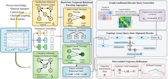
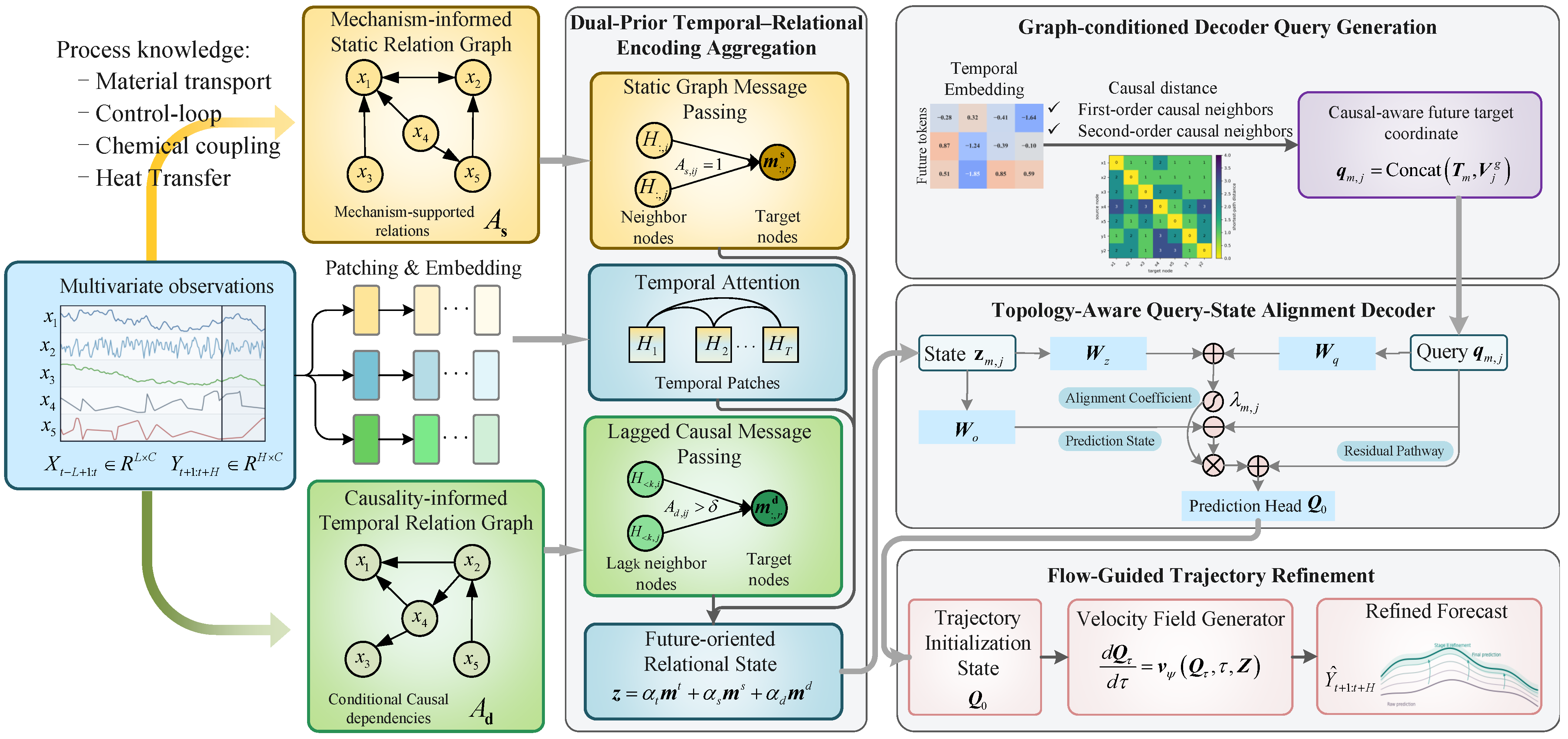
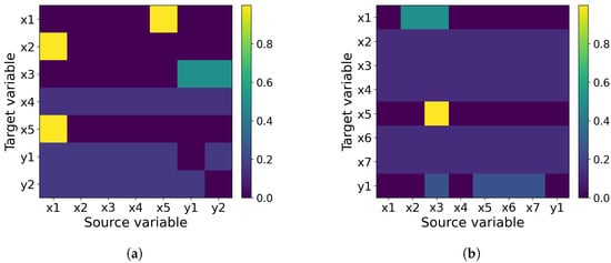
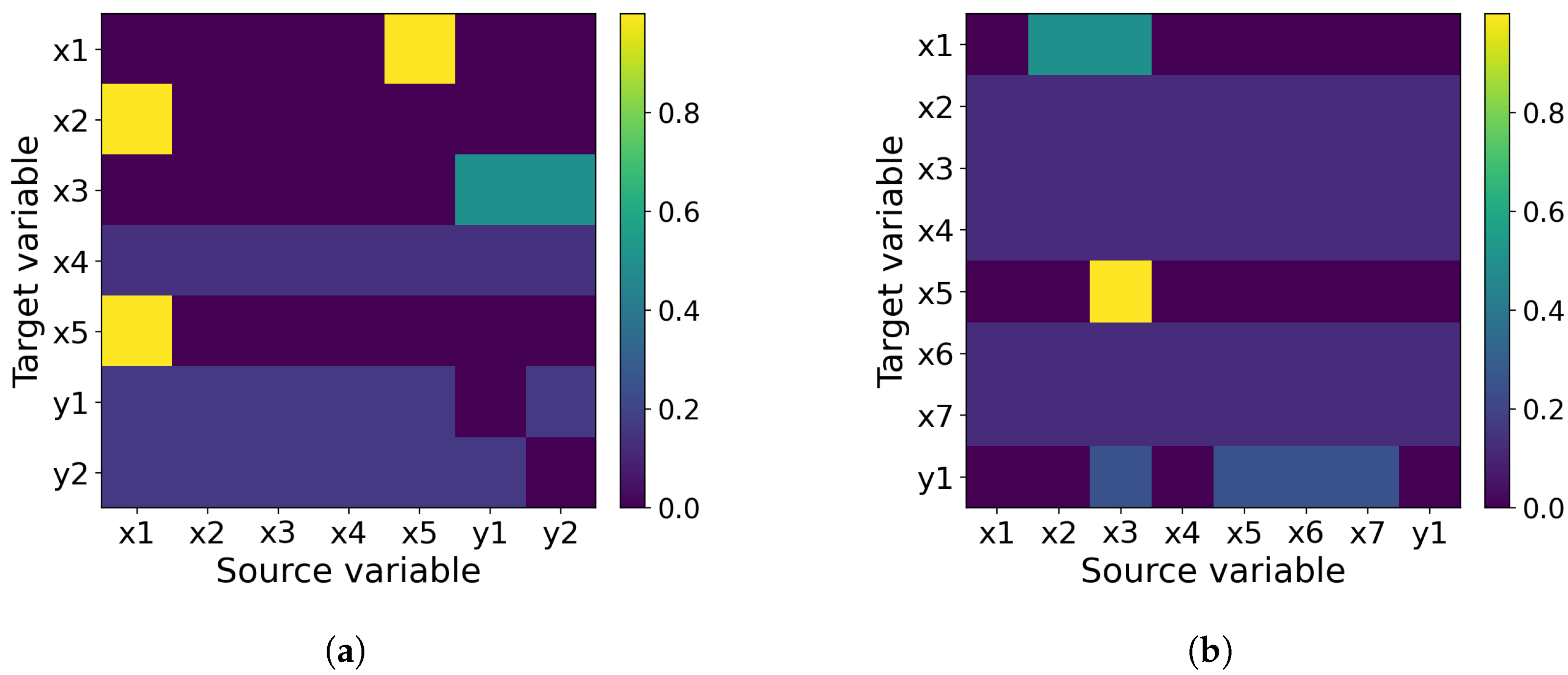
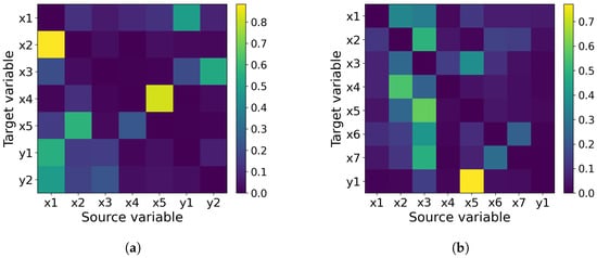
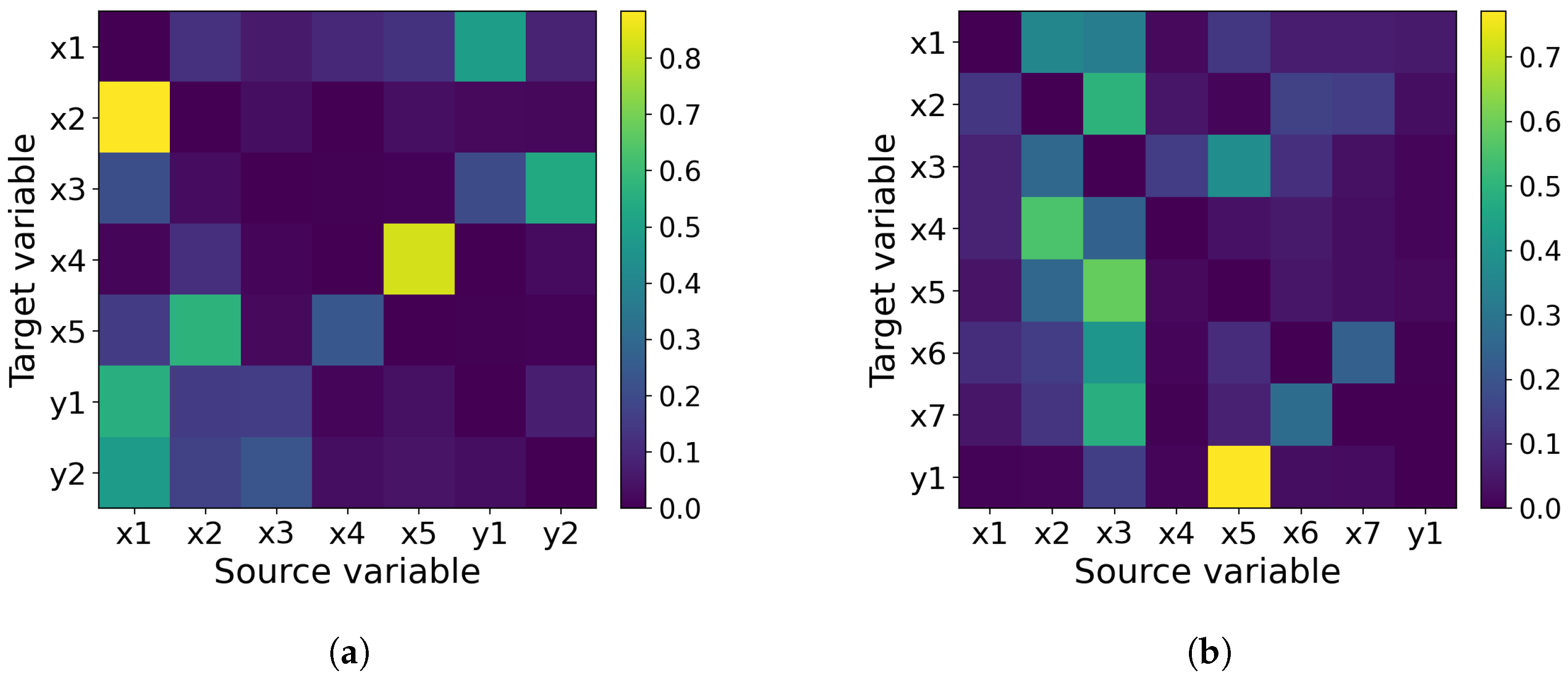
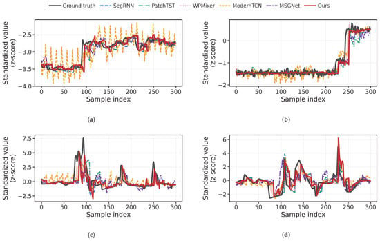
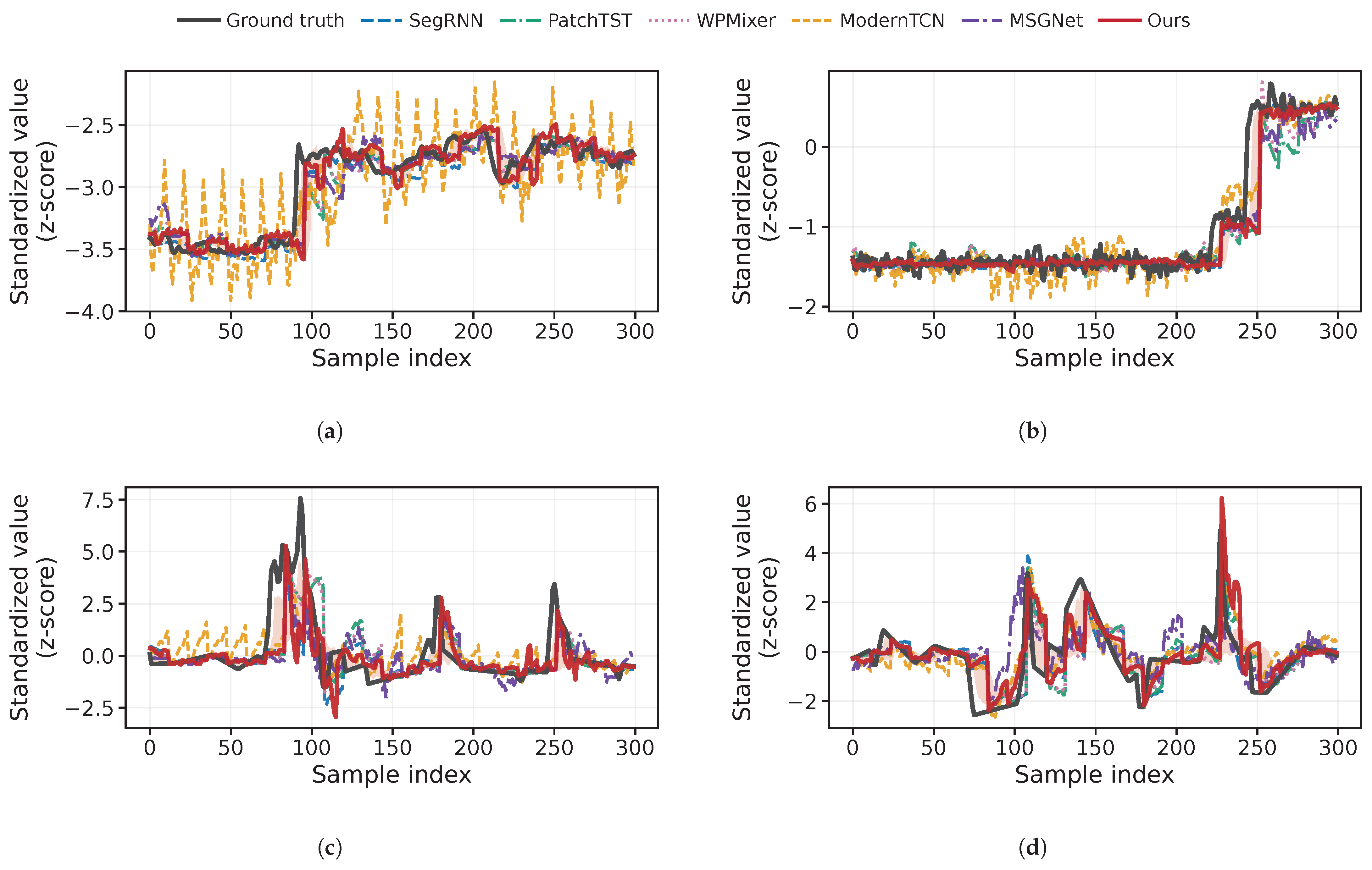
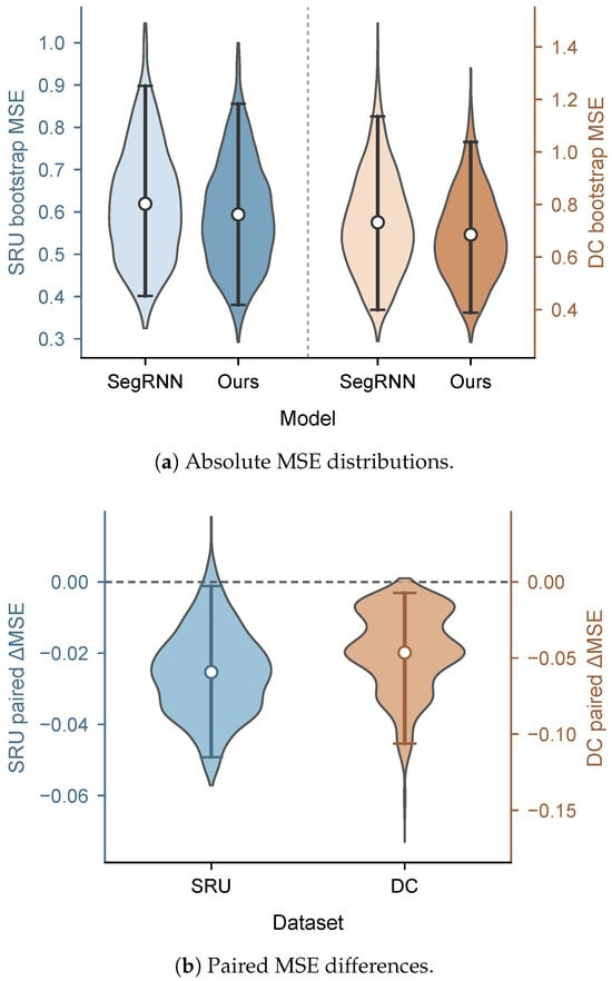
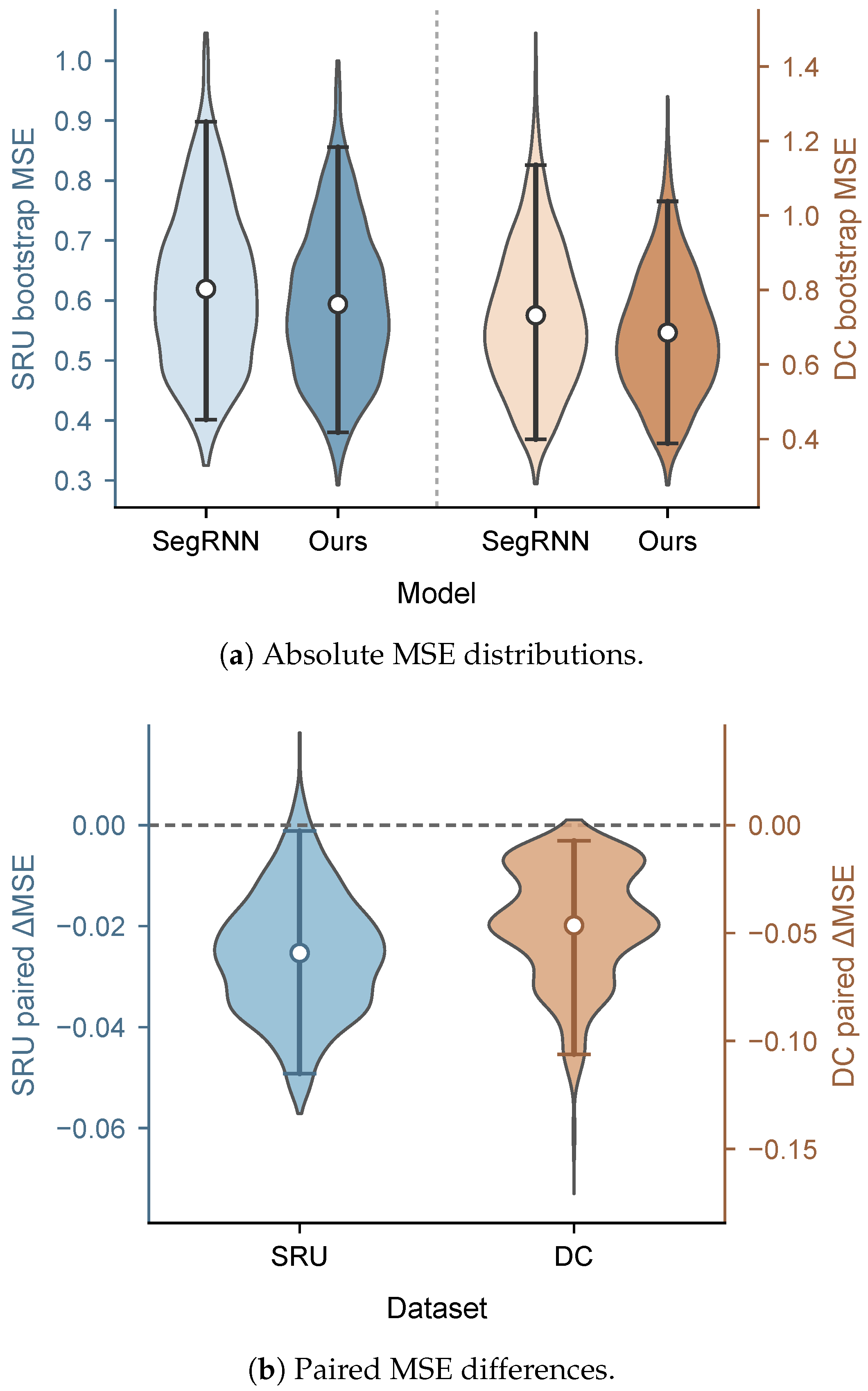
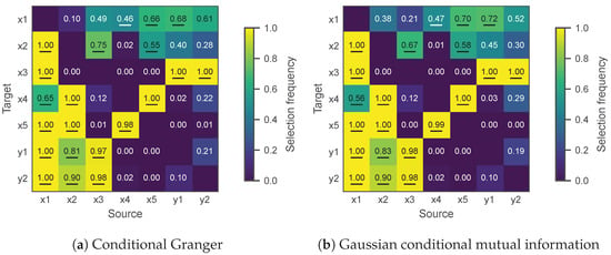
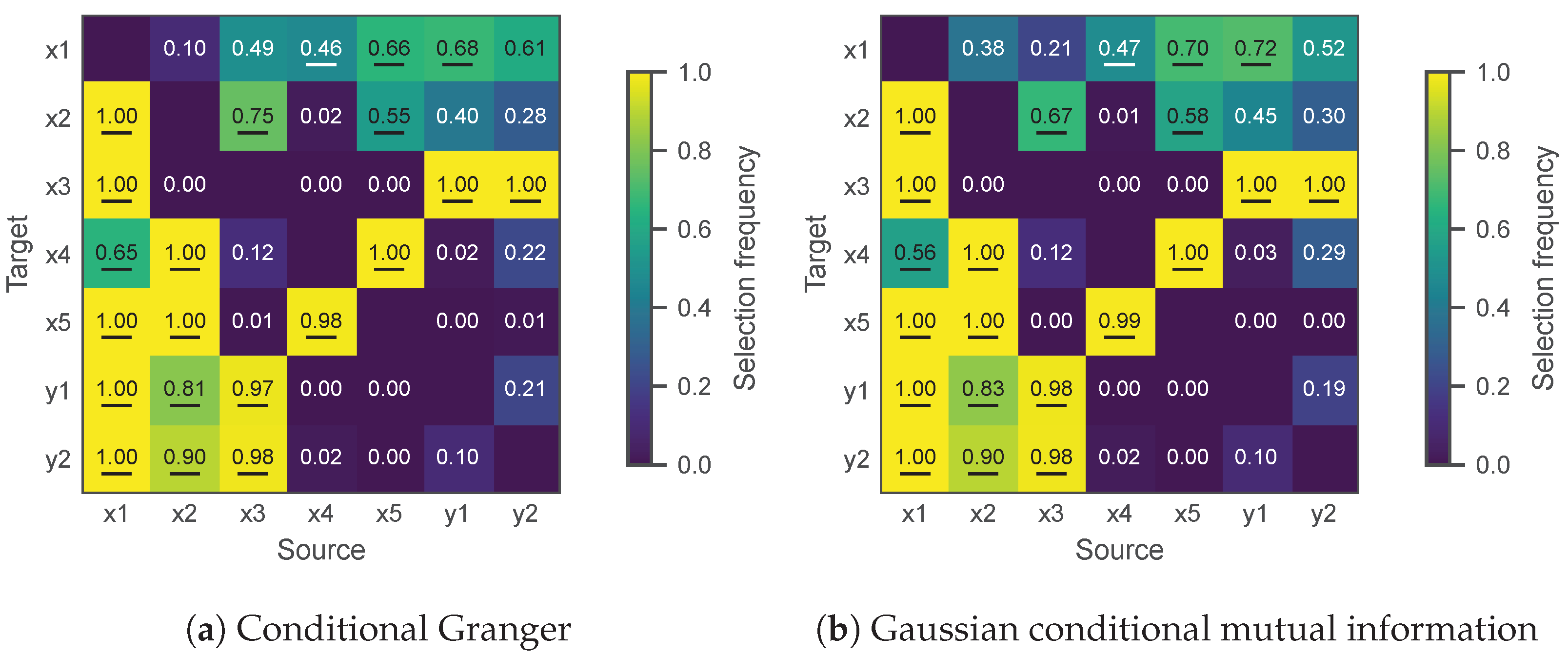
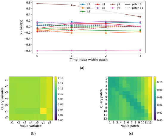
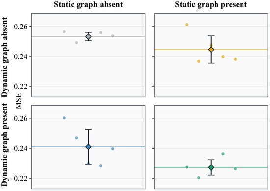
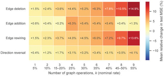
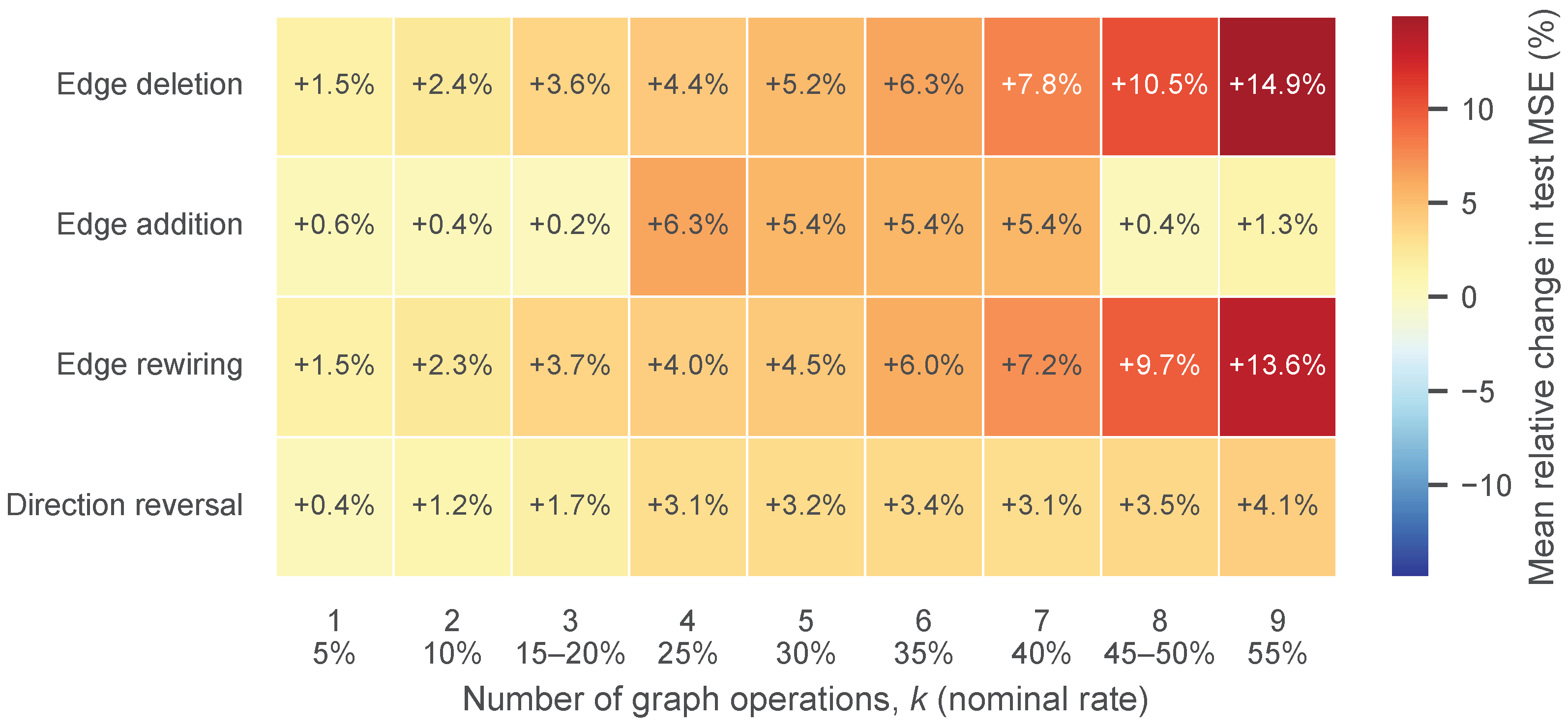
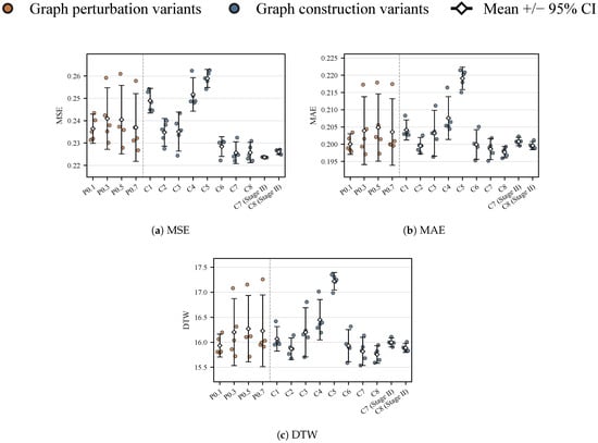
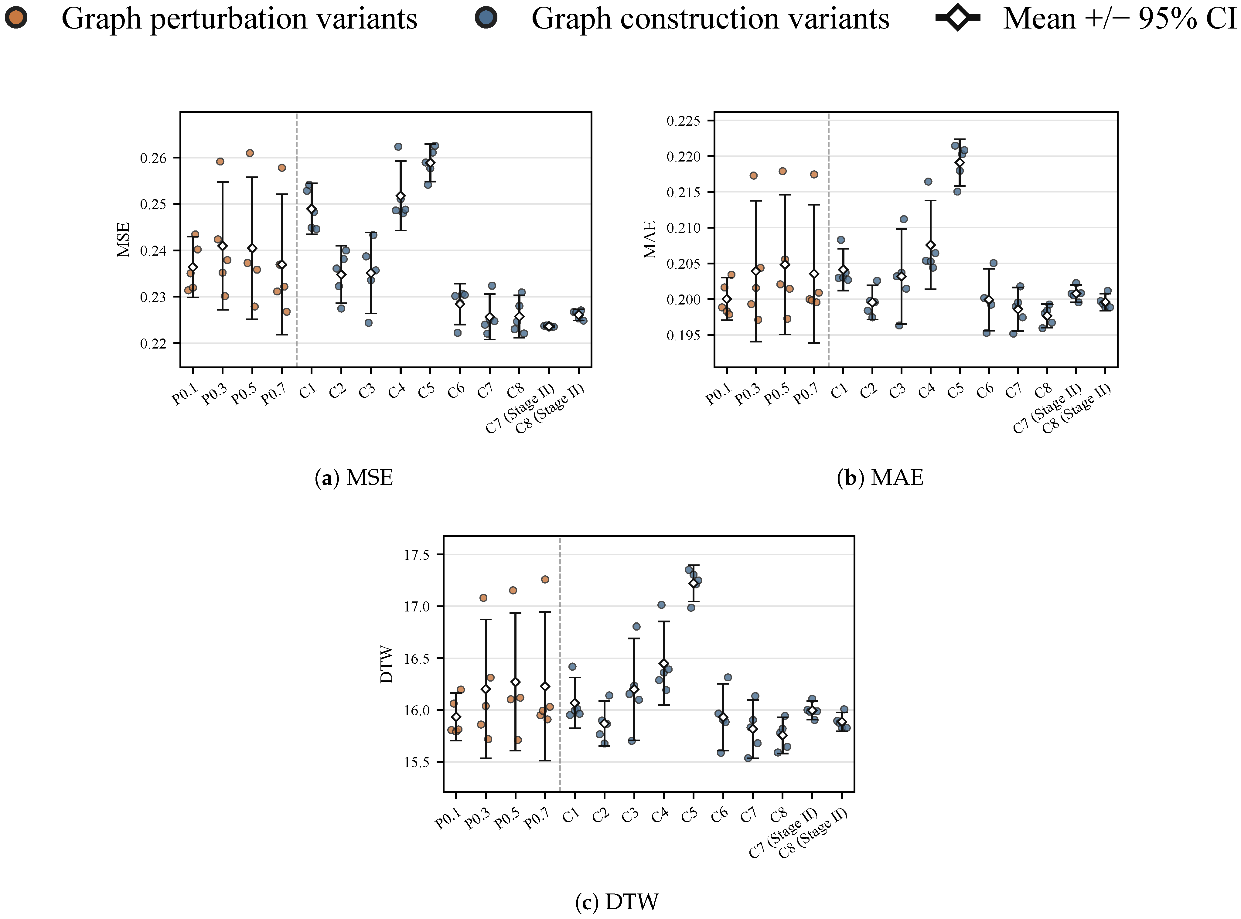
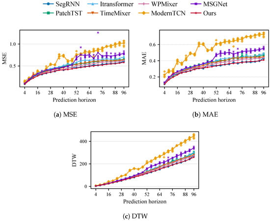
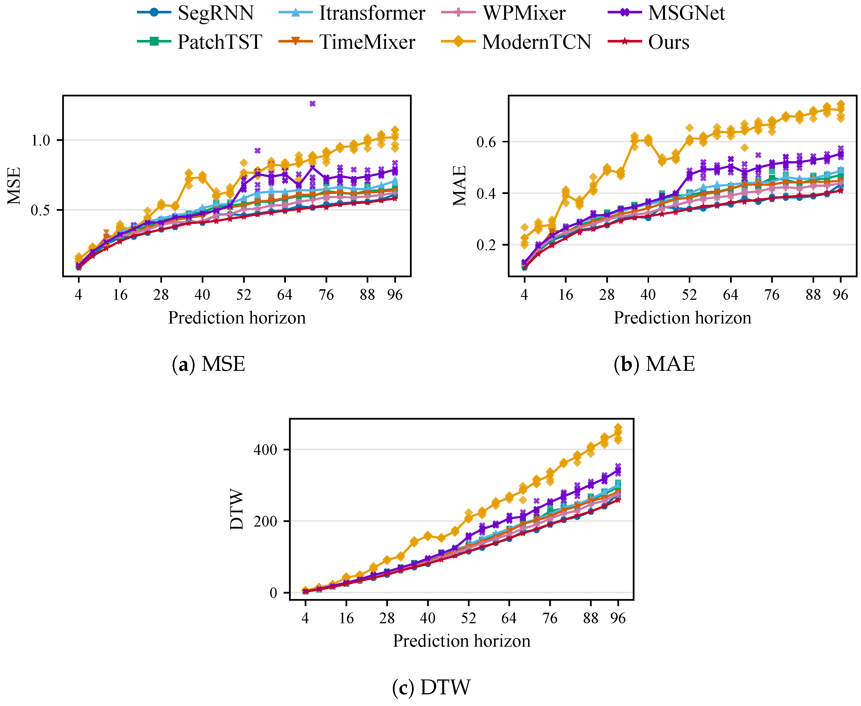
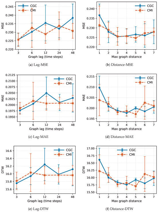
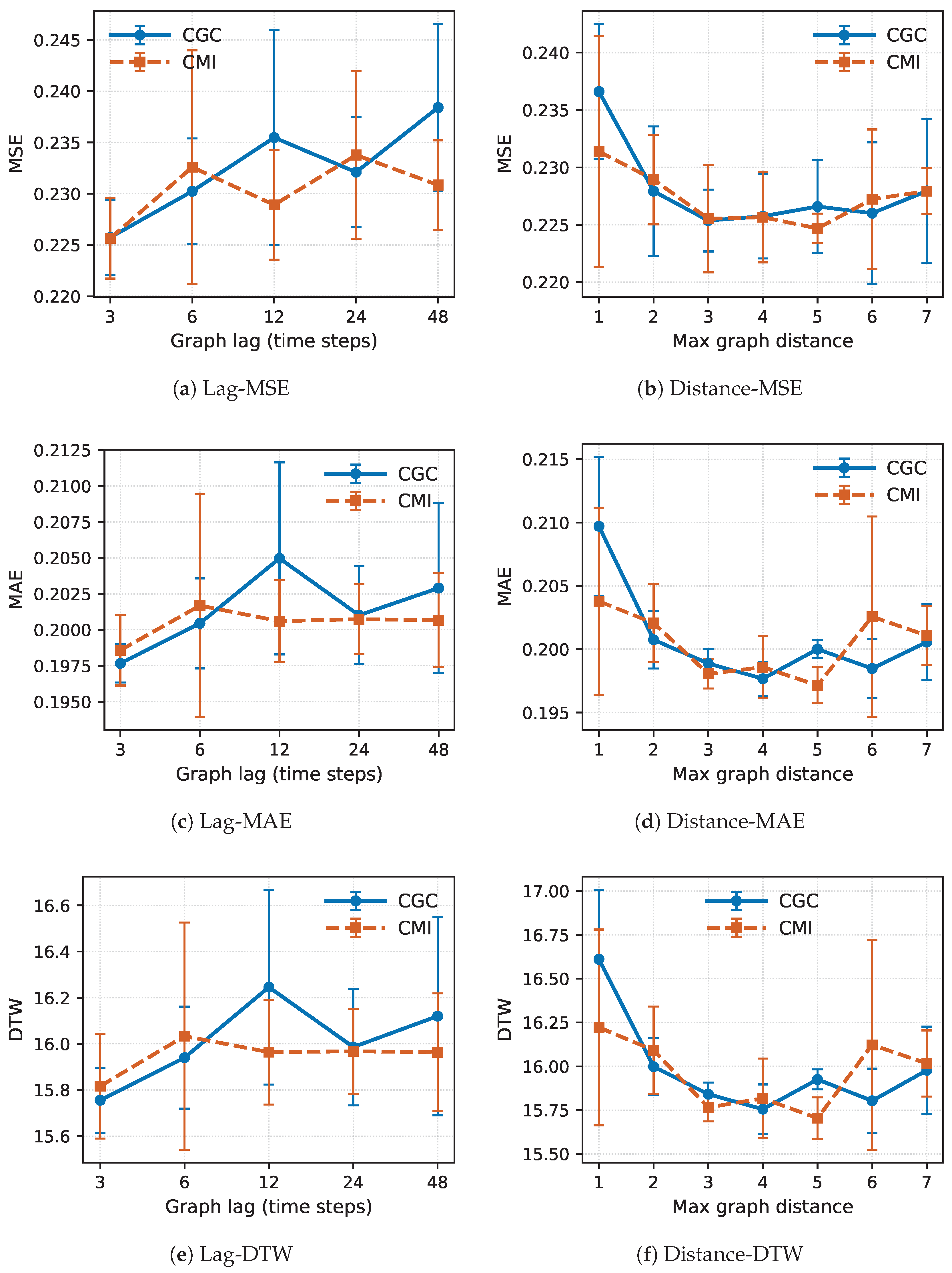
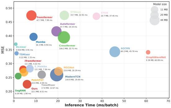
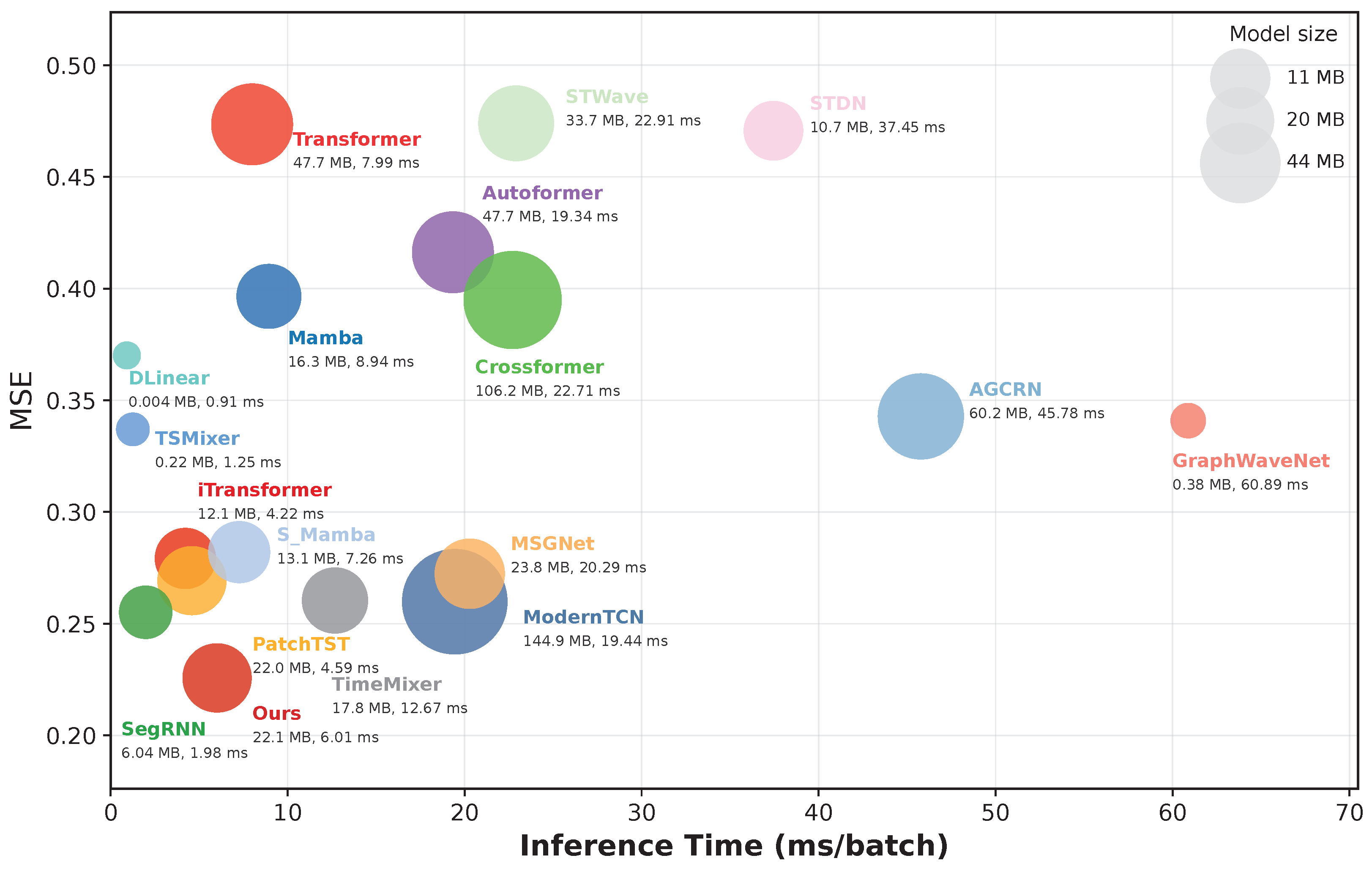

Disclaimer/Publisher’s Note: The statements, opinions and data contained in all publications are solely those of the individual author(s) and contributor(s) and not of MDPI and/or the editor(s). MDPI and/or the editor(s) disclaim responsibility for any injury to people or property resulting from any ideas, methods, instructions or products referred to in the content. |
© 2026 by the authors. Licensee MDPI, Basel, Switzerland. This article is an open access article distributed under the terms and conditions of the Creative Commons Attribution (CC BY) license.