


Abstract
Household food-waste surveys describe reported practices and attitudes but do not measure respondent-level wasted-food mass or composition. This study used a deliberately simple online questionnaire to examine digital engagement through a two-layer, benchmark-anchored framework. Among 386 respondents, 193 acknowledged household food waste: 49 ever-users of food-waste-related applications, 109 interested never-users, and 35 non-interested never-users. The observational layer examined associations with reported ever use and stated future interest through adjusted logistic regression. A separate, explicitly conditional modeling layer combined a published edible-food-waste mass benchmark, 12 external category shares and impact coefficients, and question B3 identifying the food category wasted most frequently. Reported ever use was associated with a fresh-produce B3 response (adjusted OR = 8.29; 95% CI: 2.95–23.29); the future-interest model showed limited cross-validated discrimination (AUC = 0.606). At the illustrative scenario setting τ = 2, modeled economic and carbon intensities were 2.85% and 3.24% lower for ever-users than for non-interested never-users. Excluding rare B3 responses attenuated the economic and carbon contrasts by 40.6% and 47.1%, respectively; the basic bootstrap carbon interval included zero. These conditional contrasts reflect the selected frequency-to-composition assumption and common mass benchmark, not observed changes in food-waste mass or demonstrated benefits from application use. The framework provides a transparent, reproducible exploratory bridge between questionnaire profiles and published environmental parameters.
1. Introduction
Household food waste has become a central sustainability concern because it combines social, economic, and environmental losses within the same downstream phenomenon [1,2]. The most recent global assessment estimated that approximately 1.05 billion tons of food were wasted in 2022 across households, food service, and retail, with households accounting for about 60% of that total and an average of 79 kg per person per year [3]. These figures place household practices at the heart of efforts to achieve Sustainable Development Goal 12.3. The problem is especially consequential because food discarded at the consumption stage has already embodied upstream investments in land, water, energy, labor, and other resources used throughout the food supply chain, together with the associated environmental burdens. Food loss and waste is therefore increasingly understood not merely as a disposal issue, but as the outcome of inefficiencies and resource losses occurring across the food supply chain [1].
Household food waste is also compositionally heterogeneous. Evidence from both survey-based and direct-measurement studies shows that individual food categories contribute differently to total household food waste. Perishable items such as fresh fruit and vegetables, together with bakery products, meals, and dairy products, often represent important fractions, although their relative importance varies across study settings and measurement designs [4,5]. This heterogeneity matters because kilograms of wasted food are not economically or environmentally equivalent. Food categories differ substantially in monetary value and carbon-footprint coefficients, so identical masses of different foods can generate different economic losses and climate burdens. Recent Italian evidence has shown that the economic and environmental consequences of household food waste vary strongly by food category, with some categories contributing disproportionately to monetary value and environmental impacts despite not being the largest contributors by mass [6].
A major challenge, however, is how household food waste is measured. Questionnaires remain widely used and are valuable for capturing perceptions, routines, and food-related behaviors, but their suitability for quantifying household food-waste mass is limited [7]. Italian evidence shows that questionnaire-based estimates can substantially underestimate quantities when compared with diary-based records and, where available, waste-sorting analysis [7,8]. Research comparing self-reported food waste with physically measured avoidable food waste has also found only weak correspondence between the two and has shown that variables associated with self-reported waste do not necessarily coincide with those associated with measured waste [9]. Waste-composition studies further demonstrate the value of direct measurement for quantifying household food-waste flows, although the level of category detail depends on the sorting scheme adopted [10]. The methodological implication is important: survey data are valuable for characterizing perceptions and behavioral profiles, but they should not be converted uncritically into respondent-level kilograms of food waste.
The behavioral literature likewise shows that household food waste is multidimensional rather than the outcome of a single attitude or practice. Integrative and systematic reviews describe a complex set of behavioral, personal, product-related, societal, and contextual factors, including planning and shopping routines, storage, preparation, consumption practices, social norms, and household constraints [2,11]. Empirical studies have examined planning and shopping routines, mostly using self-reported food-waste outcomes [12,13], date-label understanding [14], and broader household, contextual, and behavioral characteristics using objectively measured avoidable food waste [15]. Findings are not fully consistent across studies, partly because apparent determinants may change when the outcome is measured directly rather than self-reported [9].
Simultaneously, digital tools intended to prevent, manage, or redistribute food waste have proliferated. These include surplus-rescue and redistribution platforms, household inventory and expiry-management systems, shopping and meal-planning tools, and other consumer-facing digital interventions [16,17]. Recent empirical research has begun to differentiate distinct stages and outcomes of digital engagement. Cassia and Magno [18] compared users and non-users of an anti-food-waste app to examine motivations underlying adoption and continuance intentions; Mathisen and Johansen [17] directly measured food waste before and after the use of two food-waste-related apps in a small crossover pilot; Michelini et al. [19] examined psychosocial determinants of food-sharing app use and its association with post-consumption food-waste behavior. These studies indicate that digital engagement and intervention effectiveness cannot be represented by a single outcome. European evaluation frameworks distinguish outreach and behavioral outcomes from directly measured food-waste reduction and emphasize that intervention claims should be matched to the type and quality of evidence available [16,20].
Reported ever use, stated future interest, adoption intention, continued use, behavioral outcomes, and demonstrated waste reduction should therefore be considered distinct dimensions of digital engagement and intervention assessment. More recent studies have examined how Too Good To Go users interpret app-displayed avoided-CO2eq claims [21] and how economic and sustainability motivations influence engagement with surplus-rescue platforms [22].
The available literature provides complementary evidence on household food-waste measurement through questionnaires, diaries, and waste-composition analyses [7,8,9,10], as well as on the behavioral and contextual determinants of household food-waste practices [2,11,12,13,14,15]. Research on digital tools has examined app-use experiences and measured outcomes in pilot interventions [17], motivations underlying app adoption and engagement [18,22], food-sharing behaviors and potential rebound effects [19], and users’ perceptions of app-displayed carbon information [21]. European guidance has further addressed consumer food-waste prevention strategies and intervention-evaluation frameworks [16,20]; category-specific assessments have quantified economic and environmental burdens associated with household food waste [6]. To our knowledge, and within the literature reviewed for the present study, no directly overlapping analysis simultaneously distinguishes ever-users, interested never-users, and non-interested never-users of food-waste-related digital tools, links those engagement groups to the food categories reported as most frequently wasted, and translates the resulting profiles into category-sensitive economic and carbon scenarios while keeping total waste mass anchored to an external measurement benchmark rather than inferring it from questionnaire responses.
To address this methodological challenge, the present study develops a two-layer analytical framework connecting observed survey evidence with benchmark-anchored economic and carbon-impact scenarios. The first layer examines the sociodemographic and food-waste characteristics associated with reported ever use of food-waste-related applications and, separately, the factors associated with future interest among never-users. The second layer combines an externally measured edible household food-waste benchmark with the food categories respondents identified as most frequently wasted to generate composition-sensitive economic and carbon impact scenarios without estimating individual waste mass from expenditure, perceptions, or behavioral drivers. The methodological contribution is the explicit accounting of these assumptions and the strict separation from observed behavioral associations.
The study addresses three research questions: (1) Which sociodemographic characteristics and reported food-waste profiles are associated with previous experience of food-waste-related applications? (2) Which factors are associated with future interest among respondents who have never used these applications? (3) How do the observed B3 response profiles translate into benchmark-anchored economic and carbon-impact scenarios, and how sensitive are the resulting group contrasts to sampling variability and modeling assumptions? By separating measurement from modeling while connecting digital engagement to category-specific impact implications, the study seeks to contribute to household food-waste research and to the rigorous evaluation of digital food-waste interventions.
2. Materials and Methods
2.1. Study Design, Questionnaire, and Analytical Groups
A cross-sectional online survey was conducted using Google Forms between 13 December 2024 and 24 March 2025. The final dataset comprised 386 respondents and constituted the master dataset from which all analytical populations were derived. Participants were recruited through social networks using a non-probability sampling approach, without formal eligibility restrictions. The distribution of recruitment channels, geographical coverage, and technical duplicate-response checks was not systematically documented. For analytical purposes, the questionnaire items were organized into four thematic domains (A–D), covering sociodemographic characteristics, household food-waste practices, digital engagement, and additional app-related information. Their content, routing, and analytical use are summarized in Supplementary Table S1.
Section A collected sociodemographic information, including age, gender, household composition, educational attainment, and employment status. Section B investigated household food-waste perceptions and practices. Question B1 asked respondents whether they believed that food was wasted in their household, without providing a preliminary definition of food waste or distinguishing between edible and inedible fractions.
Respondents answering B1 = “Yes” were subsequently asked about weekly expenditure on food and beverages (B2), the food category they wasted most frequently (B3), and five perceived food-waste drivers (B4): products reaching their expiry date, excessively large portions, inadequate storage, insufficient planning, and promotions leading to over-purchasing. Question B3 was a mandatory single-response item with five predefined categories: bread and cereals, fresh fruit, fresh vegetables, meat and fish, and dairy products. An additional “Other” option allowed free-text responses. The original B3 responses, including respondent-generated entries, were retained for the subsequent analytical mapping. No standardized recall period or direct measurement of discarded-food quantities was associated with this question.
Section C addressed digital engagement with food-waste-related applications. Question C1 asked whether respondents had ever used such applications, while C2 assessed future interest among those reporting no previous use. Among interested never-users (C1 = “No”, C2 = “Yes”), question C3 collected five-point importance ratings for application features related to food-stock monitoring and expiry-date notifications, recipe suggestions, storage and portion advice, environmental-impact information, and discounted surplus-food offers. Section D collected additional descriptive information on applications previously tried, attractive functions, and perceived food-waste reductions. The C3 ratings and Section D responses were retained for descriptive purposes and were not included as predictors in the primary adjusted regression models or as inputs to the benchmark-anchored impact scenarios. Reported reductions in food waste were interpreted as respondents’ perceptions and were not treated as objectively measured outcomes.
The app-related analytical population comprised the 193 respondents answering B1 = “Yes”, representing 50.0% of the complete survey sample. Three mutually exclusive digital-engagement groups were defined according to C1 and C2: ever-users (U; n = 49), interested never-users (I; n = 109), and non-interested never-users (N; n = 35). Thus, 49 respondents reported previous app-use experience, whereas 144 reported never having used these applications, of whom 109 expressed future interest. Question C1 identified whether an application had ever been used, without establishing the timing, frequency, or continuity of use. Because the analytical population was selected according to respondents’ self-perception of household food waste, group comparisons were conditional on B1 = “Yes”. The proportion of ever-users within this group therefore cannot be interpreted as app-use prevalence in the complete survey sample or the wider population. The self-perception-based selection may also influence the observed associations.
The questionnaire routing, analytical populations, and two-layer framework are summarized in Figure 1. Panel A illustrates the definition of the three digital-engagement groups and the sample sizes used in the analyses; Panel B distinguishes the observed digital-engagement analyses from the benchmark-anchored economic and carbon impact model.
Figure 1.
Survey flow and two-layer analytical framework. Panel (A) shows the questionnaire routing and analytical populations, including the 193 respondents reporting household food waste and the three digital-engagement groups: ever-users (U), interested never-users (I), and non-interested never-users (N). Panel (B) distinguishes the observed digital-engagement analyses (Layer A) from the benchmark-anchored economic and carbon-impact scenarios (Layer B). Regression estimates were not used as inputs to the impact model.
For the benchmark-anchored modeling layer, household food waste was operationally defined as food, or edible parts of food, originally intended for human consumption and discarded within the household. This included edible leftovers, excess prepared food, expired products, and food that spoiled before consumption. Unavoidable inedible fractions, such as bones, shells, and pits, were outside the scope of the external edible-food-waste benchmark. This analytical definition was distinct from the general wording of B1, allowing for possible differences in how respondents interpreted household food waste. The impact model used the B3 responses and a common external mass benchmark to construct conditional food-category compositions without estimating respondent-specific total waste quantities from the questionnaire.
Before analysis, the working dataset was audited against the original Google Forms export. The previously extracted model inputs were compared row by row with the original responses for B2, B3, and all five B4 items, and no discrepancies were identified. Missing values were not imputed, and analyses involving incomplete variables used the available observations for each specification. One respondent selecting “Prefer not to answer” for gender was retained in the descriptive analyses but excluded from the adjusted gender-coded regressions, yielding sample sizes of 192 for the ever-use model and 143 for the future-interest model. Complete responses to all five B4 items were available for 167 respondents; these items were examined separately, using the observations available for each analysis. All 193 respondents in the app-related branch were retained for the benchmark-anchored impact model because its inputs did not require complete B4 information. Missing-data mechanisms were not empirically established, and no assumption of missing completely at random was made.
2.2. Variable Coding and Observed Digital-Engagement Analysis
Age was analyzed as a continuous variable and expressed per ten-year increase in the regression models. Gender was coded as female versus male. Household composition was collapsed into one-person, two-person, and three-or-more-person households, with the latter used as the reference category. Educational attainment was dichotomized as university degree or higher versus lower educational attainment.
Weekly expenditure on food and beverages (B2) was recorded in four household-level categories: <EUR 50, EUR 50–90, EUR 90–120, and >EUR 120. In the ever-use model, expenditure was treated as a categorical predictor, with EUR 50–90 as the reference category, allowing separate estimates across expenditure bands. In the future-interest model, an ordinal specification was adopted to limit the number of parameters, given the smaller non-interested group (n = 35). Household size was included separately in both models; expenditure referred to total household spending.
Raw B3 responses were retained for the benchmark-anchored impact model. For the observed ever-use regression analysis, sparse categories were avoided by defining a parsimonious binary variable distinguishing respondents reporting fresh fruit or vegetables as the food category they wasted most frequently from those reporting all other categories. This variable is referred to hereafter as the fresh-produce B3 profile. For descriptive purposes, B3 responses were also grouped into four broad categories: bread/cereals, vegetables, fruit, and other foods. The bread/cereals category included the “bread and cereals” response and the two pasta responses; all remaining responses other than vegetables and fruit were classified as other foods. This four-category grouping was used exclusively for descriptive comparisons and Figure 2 and was not included in either regression model or the benchmark-anchored impact model. Question B3 recorded the category reported as most frequently wasted, without measuring discarded quantities; its translation into modeled composition shares was based on the assumptions described in Section 2.3.
Figure 2.
Distribution of the most frequently wasted food categories (B3) across digital-engagement groups. Bars show the percentage of respondents reporting bread/cereals, vegetables, fruit or other foods. The overall four-category distribution and the binary fresh-produce comparison differed across groups (both p < 0.001). Percentages refer to reported food categories.
The five B4 items were initially assessed as potential components of a composite behavioral scale. Internal consistency was evaluated using Cronbach’s alpha. Because the assessment did not support a sufficiently coherent unidimensional construct, the items were retained as separate perceived food-waste drivers, and no combined behavioral index was calculated.
Descriptive comparisons across the three digital-engagement groups were conducted using the Kruskal–Wallis test for age and chi-square tests for categorical variables. The single “Prefer not to answer” response was excluded from the gender comparison. Age was summarized using mean and standard deviation and median and interquartile range, whereas categorical variables were summarized using counts and percentages. The complete variable coding scheme, analytical populations, and model-specific sample sizes are summarized in Supplementary Table S2. Sparse contingency-table cells can compromise asymptotic chi-square approximations, particularly for household size, expenditure, and the four-category B3 profile. Expected cell frequencies were examined and supplemented with Monte Carlo permutation tests, as detailed in Supplementary Table S17. These tests assess sample associations, not population representativeness.
Two binary logistic regression models were fitted. The first examined factors associated with reported ever use among respondents in the app-related branch. After exclusion of the single gender non-response, the adjusted ever-use model included 192 respondents. The final model included age, gender, household size, educational attainment, weekly food expenditure, and the fresh-produce B3 profile. The ever-use model included 49 events for nine predictor coefficients (approximately 5.4 events per coefficient), requiring caution about precision and stability. The fresh-produce odds ratio describes an association with a reported waste category, not an effect of application use. Sensitivity analyses incorporating student status and penalization are reported in Supplementary Tables S12 and S19.
The second model examined future interest only among never-users. After exclusion of the gender non-response, the adjusted future-interest model included 143 respondents. Predictors were age, gender, household size, educational attainment, and weekly food expenditure. Reported ever use and future interest were modeled separately because they represent different stages of digital engagement and were not assumed to be interchangeable outcomes.
Adjusted associations were expressed as odds ratios (ORs) with 95% confidence intervals. For multi-level predictors, global contribution to model fit was additionally assessed using likelihood-ratio tests. In the future-interest model, the smaller outcome class comprised 35 non-interested respondents; this model was intended to describe associations rather than predict realized adoption. Treating household food-expenditure classes as ordinal imposed a constant log-odds increment across unequal and partly open-ended expenditure bands, and the corresponding coefficient was interpreted cautiously.
The five B4 drivers were examined individually in separate adjusted models for each outcome. Because five driver-specific tests were conducted for each outcome, p-values were adjusted using Holm’s sequential procedure.
Candidate model specifications were compared using likelihood-ratio tests, Akaike’s information criterion, Bayesian information criterion, and parsimony. Sensitivity specifications, including a quadratic age term and student status, were examined but were not retained in the final models. Multicollinearity was assessed using variance inflation factors. Model discrimination was summarized using the area under the receiver operating characteristic curve (AUC), whereas overall probabilistic performance was evaluated using the Brier score. Internal validation was conducted through repeated stratified five-fold cross-validation with 50 repetitions. For the future-interest model, the primary 50-repetition evaluation used the fixed predictor specification described above.
An intercept-only comparator was fitted on the same training partitions and evaluated on identical validation folds. Predictive performance was summarized using means and standard deviations across the 250 held-out folds.
A complementary 20-repetition stratified five-fold cross-validation (seed 12345) was conducted using the same fixed future-interest model specification and fold-wise intercept-only comparator (Supplementary Table S12).
Potentially influential observations were examined using Cook’s distance, and sensitivity analyses were performed after excluding observations with Cook’s distance greater than 4/n. Model specifications were selected using the full analytical dataset and held fixed during cross-validation, without repeating model selection within the training folds. Consequently, the reported performance estimates do not account for model-selection uncertainty. The penalized models used the original predictor encoding without additional standardization, with C = 1 and the liblinear solver (Supplementary Tables S12 and S19). The regularization parameter was fixed for this sensitivity analysis without a separate hyperparameter-optimization procedure.
Unless otherwise specified, two-sided p-values below 0.05 were interpreted as statistically significant. All statistical associations were interpreted as cross-sectional and non-causal.
2.3. Benchmark-Anchored Impact Model
The second analytical layer translated the observed B3 response profiles into composition-sensitive economic and carbon-impact scenarios. The model combined four elements: (1) an externally measured edible household food-waste benchmark; (2) an external baseline composition across food categories; (3) the food category reported as most frequently wasted (B3); and (4) category-specific economic and carbon-footprint coefficients. The common external benchmark established the total modeled waste mass; B3 informed the conditional redistribution of that mass across food categories. Weekly food expenditure (B2), perceived food-waste drivers (B4), and digital-engagement group membership were not used to determine modeled individual compositions or total waste quantities; group membership was used only to aggregate the resulting scenarios. The main model components and assumptions are summarized in Table 1; the external category parameters are reported in Supplementary Table S3. With the B3 responses and model parameters held fixed, the resulting group means are deterministic summaries of the observed response profiles and do not provide independent empirical confirmation of the group differences.
Table 1.
Key components, parameters, and assumptions of the benchmark-anchored impact model.
The total edible food-waste benchmark was set at:
based on the Italian diary study by Giordano et al. [8]. The diary-based reference was derived from an Italian investigation conducted in May–June 2017 among 388 households, covering avoidable and possibly avoidable edible household food waste. The same study provided the baseline composition of food waste across 12 categories: vegetables, fruit, meat, cereals, baked products, dairy products, drinks, desserts, legumes, fish, eggs, and other foods. The published category masses were converted into normalized baseline shares sj such that:
Each raw B3 response was linked to the external 12-category system through a mapping matrix Hij. Direct responses were mapped to the corresponding category, whereas composite responses could activate more than one category. For example, “bread and cereals” was mapped to cereals and baked products, while “meat and fish” was mapped to meat and fish. When a response was too ambiguous to support a defensible category-specific emphasis, no personalization was applied and the respondent retained the external baseline composition. The complete primary mapping, alternative mapping rules, and their rationale are reported in Supplementary Table S5. Under the normalization in Equation (3), increasing the weight of an activated category proportionally reduces the shares assigned to the remaining categories. For example, at τ = 2, the modeled vegetable share increases from 0.2563 to 0.4080; the meat share decreases from 0.0651 to 0.0518 (Supplementary Table S6). For composite B3 responses, the same multiplier is applied to each mapped category.
A category-emphasis parameter τ controlled the strength of the B3-based modification of the external baseline composition. The primary illustrative scenario was set at τ = 2, corresponding to a twofold increase in the pre-normalization weight of the activated category or categories. Following normalization, the resulting shares depend on their baseline proportions and do not necessarily double. The value τ = 1 preserves the external reference composition, while τ = 1.25, 1.50 and 1.75 represent weaker category emphasis and τ = 3 and 5 represent stronger adjustments. These values were selected to examine the sensitivity of the modeled results to different degrees of category emphasis, without assuming an empirically established relationship between reported disposal frequency and wasted-food mass. Group-level results across the complete scenario range are reported in Supplementary Table S8, while Supplementary Tables S6 and S6a provide illustrative calculations for individual B3 response profiles. The respondent-conditioned modeled category shares were calculated as:
where Hij = 1 if external category j was activated by the B3 mapping of respondent i, and Hij = 0 otherwise. The index l denotes the summation over all external food-waste categories. By construction:
The core scenario set used for the main comparative analysis was:
The modeled allocation of the common waste-mass benchmark to category j under respondent i’s B3-conditioned scenario was calculated as:
Consequently,
for every respondent-conditioned scenario. Thus, B3 modified the modeled distribution of the common external benchmark across food categories while preserving its total mass. The resulting category masses represent conditional scenario allocations.
2.4. Economic and Carbon Impact Indicators
Category-specific economic coefficients Pj, expressed in EUR kg−1, were reconstructed from the category-level economic assessment of Italian household food waste reported by Antonelli et al. [6]. For each food category, Pj was obtained as the ratio between the published annual monetary value of wasted food and the corresponding annual wasted-food quantity. The monetary values used by Antonelli et al. [6] were based on the average of median food prices across the selected Italian provinces. The resulting category-specific coefficients used in the present model are reported in Supplementary Table S3. The coefficients for eggs (22.030 EUR/kg) and fish (3.896 EUR/kg) were verified against the published monetary values and food-waste quantities. In Antonelli et al. [6], the egg price was derived from the Milan observations and applied to the other provinces; the fish category included fresh and processed products, such as canned tuna and frozen fish fingers, as documented in Supplementary Table S1 of Antonelli et al. [6]. These characteristics of the original price data and product classification are relevant to the interpretation of the category-specific coefficients.
The source monetary and waste-mass inputs used to calculate the coefficients, together with their units, are provided in Supplementary Table S15.
Category-specific carbon-footprint coefficients CFj, expressed in kg CO2eq kg−1 food, were reconstructed from the mean category-level carbon burdens reported by Antonelli et al. [6]. For each category, the published mean weekly carbon burden was divided by the corresponding weekly wasted-food mass. Antonelli et al. [6] derived the underlying food-item carbon-footprint data from the SU-EATABLE LIFE database developed by Petersson et al. [23]. The SU-EATABLE LIFE database harmonizes life-cycle-based carbon-footprint estimates across food commodities and supply-chain stages. Its system boundaries exclude post-market processes such as household cooking and waste disposal. Accordingly, the CFj coefficients used here represent the embodied carbon burden associated with producing and supplying food that is subsequently wasted. The coefficient set is fixed across respondents and is not independently validated for this sample or survey period. A common multiplier on all CF values is only a scale check. Independently varying category-specific coefficients is evaluated in Supplementary Table S16 using explicitly hypothetical ±20% and ±50% ranges.
For each respondent (i), economic intensity was calculated as:
where EIi is expressed in EUR kg−1 of wasted food.
Carbon intensity was calculated as:
where CIi is expressed in kg CO2eq kg−1 of wasted food.
Because pij sums to one, EIi and CIi represent composition-weighted average economic and carbon intensities for the modeled wasted-food profile of respondent (i). These intensity indicators were treated as the primary comparative outcomes because they capture composition-driven differences independently of the common total-mass benchmark q0.
The corresponding benchmark-scaled economic loss was calculated as:
and the benchmark-scaled greenhouse-gas burden as:
where ELi is expressed in EUR person−1 week−1, and GHGi in kg CO2eq person−1 week−1.
Group-level indicators were calculated by averaging the modeled economic and carbon intensities (EIi and CIi), and the corresponding benchmark-scaled outputs (ELi and GHGi) within the three digital-engagement groups: ever-users (U), interested never-users (I), and non-interested never-users (N). Pairwise comparisons were performed for U–I, U–N, and I–N. Absolute contrasts were calculated as the difference between group means, with the second group used as the reference for relative percentage differences:
where and denote the group means for the metric under comparison. Negative values therefore indicate a lower modeled intensity in the first group relative to the second.
2.5. Model Validation and Uncertainty Analysis
Model validation and uncertainty analysis addressed mathematical consistency, sampling variability, structural uncertainty in the B3-to-category mapping, and sensitivity to external model parameters. The procedures and corresponding settings are summarized in Supplementary Table S4. Mathematical consistency checks verified the internal coherence of the model; the uncertainty and sensitivity analyses examined the stability of its conditional results under alternative sampling realizations and modeling assumptions. Empirical validation against directly measured household food-waste composition was not undertaken.
Mathematical consistency was first verified for every respondent and every value of Respondent-specific category shares were required to sum to one, and the corresponding modeled category masses were required to sum to the common benchmark (q0). Baseline invariance was also verified: at , all respondents were required to have identical economic and carbon intensities, irrespective of B3 response or digital-engagement group. These checks ensured that any differences observed for arose exclusively from the modeled composition adjustment.
Sampling uncertainty was evaluated using 10,000 non-parametric bootstrap replicates, with replacement resampling performed separately within the ever-user (U), interested never-user (I), and non-interested never-user (N) groups to preserve their original sample sizes. For each replicate and value of τ, group mean economic and carbon intensities and the U–I, U–N, and I–N contrasts were recalculated from the resampled B3 profiles. The bootstrap analysis for the primary scenario (τ = 2) used NumPy’s PCG64 pseudorandom number generator with seed 4620418. Percentile-based 95% confidence intervals and directional bootstrap frequencies were calculated. These intervals were exploratory and unadjusted for multiple pairwise comparisons; directional frequencies described the proportions of resamples exhibiting a specified contrast sign.
An additional analysis of the U–N contrasts at τ = 2 used 20,000 stratified bootstrap replicates to compare percentile, bias-corrected and accelerated (BCa), and basic confidence intervals. The calculations were reconstructed from the published B3 group frequencies, primary mapping rules, and category coefficients, as documented in Supplementary Table S20.
Structural model uncertainty was evaluated separately by varying the B3-to-category mapping rules. Nine ambiguous or composite B3 response types had more than one defensible mapping, as detailed in Supplementary Table S5. Exhaustive combination of the alternative rules generated 1728 distinct mapping configurations. Each configuration was evaluated at , and , yielding 5184 complete structural configurations. The 1 scenario was excluded because the modeled composition is invariant to the B3 mapping when no category emphasis is applied. The external baseline composition, category coefficients, and multiplicative adjustment rule in Equation (3) were held fixed across these configurations.
For each structural configuration, the U–N contrasts in economic and carbon intensity and the ordering of the three group means were recalculated. Structural robustness was summarized as the frequency with which the direction of the U–N contrast and the observed group ordering were preserved across the predefined model space. These frequencies describe robustness to alternative defensible modeling assumptions. The U–N endpoint contrast was emphasized after inspection of its relative stability; it should therefore be read as an exploratory focus. The extreme contrasts and corresponding mapping configurations identified through the full-factorial analysis are reported in Supplementary Table S11.
Sensitivity to category-specific economic and carbon-footprint coefficients was examined through independent multiplicative perturbations of the twelve economic coefficients and the twelve carbon coefficients. Two hypothetical ranges were considered, Uniform (0.8, 1.2) and Uniform (0.5, 1.5), with 50,000 draws per range and a fixed random seed (2702026). These analyses assessed the direction and magnitude of the U–N contrasts under heterogeneous coefficient changes. The perturbation ranges were defined as exploratory stress tests (Supplementary Table S16).
Scale sensitivity was examined independently from sampling and structural uncertainty. First, the external food-waste benchmark (q0) was increased by 20%, following the approximate diary under-recording discussed by Giordano et al. [8] on the basis of an earlier pilot study.
Second, economic-coefficient sensitivity was assessed by applying a common price multiplier ranging from 0.931 to 1.121 to all Pj values, based on the territorial variation in median-price monetary values reported by Antonelli et al. [6]. The multiplier was applied uniformly to the twelve economic coefficients (Pj).
Third, an exploratory carbon-scale sensitivity analysis was performed using a common multiplier of 0.616, corresponding to the ratio between the published median and mean total carbon footprints reported by Antonelli et al. [6]. This aggregate ratio was applied uniformly to the 12 carbon-footprint coefficients to examine the effect of a proportional change in the overall carbon-impact scale while preserving the relative relationships among category coefficients.
By construction, increasing q0 proportionally changes the benchmark-scaled economic losses (EL) and greenhouse-gas burdens (GHG) without affecting the corresponding intensities (EI and CI). Similarly, applying a positive common multiplier to all economic or carbon coefficients proportionally rescales the respective intensity and benchmark-scaled indicators. These adjustments preserve relative group contrasts and group ordering within each indicator.
2.6. Software
Data preparation, descriptive and regression analyses, mathematical consistency checks, cross-validation, bootstrap resampling, structural mapping enumeration, sensitivity analyses, and calculation of the benchmark-anchored impact scenarios were performed in Python 3.13.5. The principal analytical libraries were pandas 2.2.3, NumPy 2.3.5, SciPy 1.17.0, statsmodels 0.14.6, scikit-learn 1.8.0, and Matplotlib 3.10.8. Survey-based analyses used the observed respondent data without population weighting; the benchmark-anchored impact model additionally incorporated external food-waste and impact parameters. The Supplementary Materials provide the equations, external parameters, B3 response frequencies, mapping rules, and worked calculations needed to reproduce the benchmark-anchored impact scenarios and group-level bootstrap comparisons. The corresponding Python implementation and the computational procedure for the bootstrap analyses are provided in the Supplementary Material. Reproduction of the observational regression analyses requires respondent-level covariates and outcomes, subject to the data-access conditions described in the Data Availability Statement.
3. Results
3.1. Sample Structure and Digital Engagement
Of the 386 survey respondents, 193 (50.0%) reported household food waste and entered the app-related branch of the questionnaire. Among these respondents, 49 (25.4%) reported having previously used food-waste-related applications and were classified as ever-users (U). The remaining 144 respondents had never used such applications. Among these never-users, 109 (75.7%) expressed interest in trying them in the future and were classified as interested never-users (I), whereas 35 (24.3%) reported no such interest and were classified as non-interested never-users (N). Comparisons between the two B1 branches were restricted to the demographic information available for all respondents.
In the complete survey sample, respondents answering B1 = “Yes” were younger on average than those answering B1 = “No” (40.32 versus 45.32 years; Mann–Whitney p = 0.0010). University-level education was also more frequent among respondents reporting household food waste (162/193 versus 139/193; χ2 p = 0.0147). These differences indicate that the two B1 response groups differed in their demographic composition. Additional descriptive counts are provided in Supplementary Table S13.
The three digital-engagement groups differed in age, educational attainment, weekly food expenditure, and reported B3 profiles (Table 2). Ever-users were the youngest group, with a median age of 27 years, compared with 44 years among interested never-users and 42 years among non-interested never-users (Kruskal–Wallis H = 18.11, p < 0.001). No statistically significant group differences were detected for gender or household size at the conventional 0.05 threshold.
Table 2.
Characteristics of respondents by digital-engagement group.
Complete responses to all five B4 items were available for 167 respondents (86.5%), with similar completeness across ever-users (85.7%), interested never-users (86.2%), and non-interested never-users (88.6%; p = 0.923). Among ever-users, 47 of 49 respondents (95.9%) reported having tried Too Good To Go, either alone or together with another application. Regarding perceived food-waste reduction, 5 ever-users (10.2%) reported a substantial reduction attributed to app use, 32 (65.3%) reported a limited reduction, and 12 (24.5%) reported no reduction.
3.2. Observed Food-Waste Profiles and Perceived Waste Drivers
B3 response profiles differed markedly across the three digital-engagement groups (Figure 2). Fresh fruit or vegetables were reported as the most frequently wasted food category by 79.6% of ever-users, compared with 41.3% of interested never-users and 28.6% of non-interested never-users (p < 0.001). Conversely, bread and cereals were reported by 16.3% of ever-users, compared with 46.8% of interested never-users and 54.3% of non-interested never-users. The overall four-category B3 distribution differed across groups (p < 0.001), as did the binary fresh-produce B3 profile (p < 0.001).
The original B3 response frequencies are reported in Supplementary Table S7. Because the four-category comparison included one expected cell frequency below five, the asymptotic result was supplemented with a 5000-permutation Monte Carlo test (p ≈ 0.0002), confirming the evidence of differences across groups. The corresponding sparse-cell diagnostics and permutation tests for weekly expenditure and household size are reported in Supplementary Table S17.
The five B4 items showed limited internal consistency (Cronbach’s α = 0.566) and were examined separately. In the adjusted ever-use analyses, the lowest unadjusted p-values were observed for products reaching their expiry date (OR = 0.75; p = 0.058) and promotions leading to over-purchasing (OR = 1.31; p = 0.116). Their Holm-adjusted p-values were 0.288 and 0.463, respectively. None of the five perceived waste drivers showed a statistically significant adjusted association with either reported ever use or future interest after Holm correction. Complete results are presented in Supplementary Table S14.
3.3. Factors Associated with Reported Ever Use of Food-Waste-Related Applications
The adjusted ever-use model included 192 respondents, of whom 49 reported previous experience with food-waste-related applications. Reported ever use was inversely associated with age: for each ten-year increase, the odds of reporting previous app use were 42.5% lower (adjusted OR = 0.575, 95% confidence interval 0.411–0.805; p = 0.001). Respondents with a university degree or higher also had lower adjusted odds of reported ever use than those with lower educational attainment (adjusted OR = 0.245, 95% confidence interval 0.083–0.726; p = 0.011). Weekly food expenditure contributed significantly to model fit at the global level (likelihood-ratio p = 0.010), although the category-specific pattern was non-monotonic.
Relative to respondents spending EUR 50–90 per week, those spending more than EUR 120 had higher adjusted odds of reported ever use (adjusted OR = 5.57, 95% confidence interval 1.48–21.02; p = 0.011); the other expenditure categories were not individually associated with reported ever use. The largest observe adjusted association was found for the fresh-produce B3 profile. Respondents reporting fresh fruit or vegetables as the food category they wasted most frequently had substantially higher adjusted odds of reported ever use than respondents reporting other food categories as most frequently wasted (adjusted OR = 8.29, 95% confidence interval 2.95–23.29; p < 0.001). Gender and household size were not significantly associated with reported ever use in the adjusted model (Table 3).
Table 3.
Adjusted associations with reported ever use of food-waste-related applications.
The model showed an apparent AUC of 0.830 and a Brier score of 0.136. Repeated stratified five-fold cross-validation yielded a lower mean AUC of 0.774 and a mean Brier score of 0.159, indicating some reduction in predictive performance under internal resampling. Centered variance inflation factors were below 3.3, providing no indication of problematic multicollinearity. The direction of the principal associations was also preserved in the influence sensitivity analysis.
Sensitivity analyses examined the influence of student status and coefficient penalization on the adjusted estimates. After including student status, the odds ratio for university education changed from 0.245 to 0.256, while student status itself was not significantly associated with reported ever use (OR = 2.27; Wald p = 0.127; likelihood-ratio p = 0.125). Under L2 penalization, the odds ratios for university education, the fresh-produce B3 profile, and expenditure above EUR 120 decreased to 0.410, 5.002, and 2.899, respectively. These analyses preserved the directions of the principal associations while indicating some sensitivity in their magnitude (Supplementary Tables S12 and S19).
3.4. Factors Associated with Future Interest Among Never-Users
The adjusted future-interest model included 143 never-users, of whom 108 expressed interest in trying food-waste-related applications in the future. Female respondents had higher adjusted odds of future interest than male respondents (adjusted OR = 2.77, 95% confidence interval 1.20–6.41; p = 0.017). Respondents with a university degree or higher also had higher adjusted odds of future interest than those with lower educational attainment (adjusted OR = 3.78, 95% confidence interval 1.31–10.94; p = 0.014). Age was not significantly associated with future interest (OR = 1.29, 95% confidence interval 0.93–1.79; p = 0.134). No significant association was observed for household size (global likelihood-ratio; p = 0.784) or weekly food expenditure, which was modeled as an ordinal one-category increase (OR = 0.74, 95% confidence interval 0.44–1.26; p = 0.273) (Table 4).
Table 4.
Adjusted associations with future interest among never-users.
The future-interest model showed an apparent AUC of 0.676 and a Brier score of 0.165. Across 50 repetitions of stratified five-fold cross-validation, the fixed Table 4 specification yielded a mean AUC of 0.606 (SD = 0.111) and a mean Brier score of 0.18396 (SD = 0.02284). On the same validation folds, the intercept-only comparator yielded a mean Brier score of 0.18490 (SD = 0.00216), with a mean paired difference of −0.00094 (SD = 0.02269). This small difference indicates limited improvement in out-of-sample probability accuracy. A complementary 20-repetition analysis produced similar results, with a mean AUC of 0.603 (SD = 0.114) and Brier scores of 0.18488 and 0.18490 for the adjusted and intercept-only models, respectively (Supplementary Table S12). The reported standard deviations describe variability across validation folds. Predictor selection preceded cross-validation and was not repeated within the training partitions. Sensitivity analyses examined the stability of the educational-attainment association. After adjustment for student status, the odds ratio for university education changed from 3.783 to 3.798; the corresponding L2-penalized estimate was 2.519. The direction of the association remained positive across these specifications, although penalization attenuated its magnitude (Supplementary Tables S12 and S19). Figure 3 provides a graphical comparison of the adjusted associations identified by the two digital-engagement models.
Figure 3.
Adjusted odds ratios (ORs) and 95% confidence intervals from the multivariable logistic regression models for (a) reported ever use of food-waste-related applications and (b) future interest among never-users. Points represent adjusted ORs and horizontal lines represent 95% confidence intervals. The dashed vertical line indicates the null value (OR = 1). Odds ratios are displayed on a logarithmic scale.
3.5. Benchmark-Anchored Economic and Carbon Impact Scenarios
At τ = 1, the unchanged external reference composition yielded identical economic and carbon intensities across the three digital-engagement groups, corresponding to 5.113 EUR/kg and 2.352 kg CO2eq/kg, respectively (Table 5). Applying the common edible food-waste benchmark of 0.5299 kg/person/week, these intensities corresponded to a benchmark-scaled economic loss of 2.709 EUR/person/week and a greenhouse-gas burden of 1.246 kg CO2eq/person/week. Under the primary illustrative scenario at τ = 2, the corresponding sample-wide modeled values were 2.555 EUR/person/week and 1.149 kg CO2eq/person/week. Compared with τ = 1, these lower values reflect the redistribution of the reference food-waste composition according to the categories reported as most frequently wasted in B3. The category-weighting and normalization procedure modifies the relative contributions of foods with different economic values and carbon footprints while preserving the common waste-mass benchmark and the category-specific impact coefficients. The resulting variation illustrates how the assumed composition of household food waste influences the estimated economic and environmental burdens.
Table 5.
Modeled economic and carbon intensities across the four core category-emphasis scenarios.
At τ = 2, modeled economic intensities were 4.751, 4.831, and 4.891 EUR/kg for ever-users (U), interested never-users (I), and non-interested never-users (N), respectively. The corresponding carbon intensities were 2.131, 2.173, and 2.202 kg CO2eq/kg. Relative to group N, the modeled profile of ever-users showed a 2.85% lower economic intensity and a 3.24% lower carbon intensity.
Across the core scenarios, higher τ values yielded lower modeled economic and carbon intensities for all three groups and larger between-group contrasts (Table 5 and Figure 4). The U–N carbon-intensity contrast reached −5.73% at τ = 3 and −9.36% at τ = 5. Under the weaker-emphasis scenarios at τ = 1.25, 1.50, and 1.75, the corresponding contrasts were −0.90%, −1.74%, and −2.51%, while the economic-intensity contrasts were −0.81%, −1.55%, and −2.23% (Supplementary Table S8). The overall pattern reflects the interaction between the imposed category weighting, the distribution of reported food-waste categories, and the external reference coefficients.
Figure 4.
Modeled economic intensity (a) and carbon intensity (b) for ever-users (U), interested never-users (I), and non-interested never-users (N) across the four core category-emphasis scenarios (τ = 1, 2, 3, and 5). The τ = 1 scenario represents the unchanged external reference composition, while increasing τ modifies the modeled category shares according to the reported B3 responses. The intermediate scenarios (τ = 1.25, 1.50, and 1.75) are reported in Supplementary Table S8.
3.6. Sampling and Model Uncertainty
At τ = 2, the U–N economic- and carbon-intensity contrasts reflected differences in the modeled composition of the twelve food categories (Supplementary Table S9). Expressing the category contributions relative to the common benchmark intensities at τ = 1 (5.113 EUR/kg and 2.352 kg CO2eq/kg) provides further insight into the influence of proportional redistribution. Vegetables and fruit accounted for modeled shares that were 5.34 and 2.82 percentage points higher, respectively, among ever-users. Their carbon-footprint coefficients, both below the reference intensity, yielded centered contributions of −0.0777 and −0.0439 kg CO2eq/kg. These negative contributions were partly offset by positive centered contributions from baked products (+0.0480 kg CO2eq/kg) and cereals (+0.0289 kg CO2eq/kg). Although their modeled shares were lower among ever-users, both categories had carbon-footprint coefficients below the reference intensity, resulting in positive contributions under the reference-centered formulation. The combined redistribution across all twelve categories produced a net carbon-intensity difference of −0.0713 kg CO2eq/kg and an economic-intensity difference of −0.1394 EUR/kg.
The leave-one-out analysis yielded U–N carbon-intensity differences ranging from −0.0911 to −0.0455 kg CO2eq/kg. Greater attenuation emerged after excluding the 10 original B3 response labels occurring four or fewer times in the complete analytical sample (Supplementary Table S10). This exclusion affected thirteen responses: one ever-user, seven interested never-users, and five non-interested never-users. At τ = 2, the U–N carbon-intensity contrast decreased in magnitude from −0.0713 to −0.0377 kg CO2eq/kg (47.1%), while the economic-intensity contrast changed from −0.1394 to −0.0828 EUR/kg (40.6%). Both influence analyses preserved the negative direction of the U–N point estimates, although their magnitude was sensitive to sparsely represented B3 responses.
At τ = 2, the stratified bootstrap yielded a U–N economic-intensity difference of −0.1394 EUR/kg (95% percentile interval: −0.2504 to −0.0335) and a carbon-intensity difference of −0.0713 kg CO2eq/kg (−0.1488 to −0.0001; Table 6). A complementary analysis using 20,000 bootstrap replicates produced a BCa interval of −0.1550 to −0.0069 kg CO2eq/kg and a basic interval of −0.1419 to +0.0038 kg CO2eq/kg for the carbon contrast (Supplementary Table S20). The upper limits of these intervals illustrate the sensitivity of the carbon-intensity comparison to the interval estimation method, with the basic interval extending slightly above zero.
Table 6.
Exploratory bootstrap pairwise contrasts under the primary category-emphasis scenario ().
The U–I and I–N comparisons were less conclusive, with some pairwise bootstrap intervals including zero. The complete U < I < N carbon-intensity ordering occurred in 73.91% of bootstrap replications. Taken together, the influence and bootstrap analyses show greater consistency in the direction of the exploratory U–N point estimates than in their magnitude and statistical uncertainty. These findings characterize the behavior of the benchmark-anchored scenarios within the investigated sample and the specified modeling assumptions.
Structural uncertainty analysis provided a complementary assessment of robustness to alternative B3-to-category mapping assumptions. For each of the personalized scenarios (), all 1728 predefined mapping configurations were evaluated, yielding 5184 complete structural configurations. Across this model space, the U–N contrast remained negative for both economic and carbon intensity, and the observed-sample ordering U < I < N was preserved across the enumerated mapping configurations. The stability observed across the mapping configurations reflects the external baseline composition and coefficient values adopted in the model. Sensitivity to variations in individual category coefficients was assessed separately in Supplementary Table S16. The scenario configurations have no defensible probability weights; frequencies across the grid are not probabilities of real-world effectiveness.
Figure 5 summarizes the distribution of the U–N relative differences across the alternative mapping configurations. The full minimum-to-maximum ranges remained below zero for both indicators, indicating that the direction of the U–N contrast was not dependent on any single defensible B3 mapping specification. At τ = 2, the economic-intensity contrast ranged from −0.2089 to −0.1121 EUR/kg (−4.19% to −2.31%), while the carbon-intensity contrast ranged from −0.1147 to −0.0619 kg CO2eq/kg (−5.07% to −2.84%). The corresponding extrema for τ = 3 and τ = 5, together with the mapping configurations producing each result, are reported in Supplementary Table S11. All evaluated ranges remained negative for both indicators.
Figure 5.
Structural uncertainty in the ever-user versus non-interested never-user (U–N) contrast. Points represent the median U–N relative difference across 1728 alternative B3 mapping configurations at each personalized scenario (τ = 2, 3, and 5), while whiskers indicate the corresponding minimum-to-maximum ranges. Negative values indicate lower modeled intensity for ever-users relative to non-interested never-users. All ranges remained below zero for economic intensity (a) and carbon intensity (b). Numerical extrema and corresponding mapping configurations are reported in Supplementary Table S11.
Sensitivity to independent variation in category-specific economic and carbon coefficients was assessed at τ = 2 (Supplementary Table S16). Under the hypothetical ±20% perturbation range, the U–N contrasts remained negative in all 50,000 simulated coefficient configurations for both indicators. Under the wider ±50% range, negative contrasts were observed in 97.9% of configurations for economic intensity and 99.9% for carbon intensity. The corresponding 2.5th–97.5th percentile ranges were from −0.2749 to −0.0037 EUR/kg and from −0.1184 to −0.0244 kg CO2eq/kg, respectively. These results indicate substantial directional stability across the examined coefficient perturbations, with greater sensitivity in the economic-intensity contrast under the wider range. The perturbation bounds were hypothetical and were not interpreted as empirically calibrated uncertainty distributions. The common-scale sensitivity analyses produced proportional changes in the corresponding modeled indicators. Increasing the external mass benchmark affected the benchmark-scaled economic losses and greenhouse-gas burdens, while common economic and carbon multipliers rescaled their respective intensity and benchmark-scaled outputs. As expected from the multiplicative structure of the model, these adjustments preserved group ordering and relative percentage contrasts. Unlike the independent coefficient perturbations, common-scale adjustments could not alter the direction of the modeled group differences.
4. Discussion
4.1. Principal Findings
The present study identified distinct patterns of digital engagement among respondents acknowledging household food waste. Reported previous use of food-waste-related applications was associated with younger age and reporting fresh produce as the most frequently wasted food category; future interest among never-users showed different sociodemographic associations. The benchmark-anchored analysis connected these observed profiles to conditional economic and carbon-intensity scenarios. At τ = 2, the modeled U–N differences were −2.85% and −3.24%, respectively, under a common external waste-mass benchmark. Both contrasts remained negative across the examined alternative B3 mapping configurations. However, excluding sparsely represented B3 responses attenuated their magnitude, and the basic bootstrap interval for the carbon-intensity contrast included zero. These findings indicate that the direction of the modeled differences was relatively stable across the specified structural assumptions, while their magnitude and statistical uncertainty remained sensitive to analytical choices. The results characterize reported digital engagement and conditional impact profiles within the investigated sample, without providing evidence of an actual reduction in household food-waste quantities attributable to application use.
4.2. Digital Engagement and Household Food-Waste Profiles
The strong age gradient in reported ever use can be interpreted in light of research examining younger consumers as a heterogeneous population in food-waste prevention. Studies on Italian youth have highlighted the combined influence of planning, purchasing, consumption, and awareness-related practices on household food waste [24]. In the present sample, younger respondents were more likely to report previous experience with food-waste-related applications. This association may reflect differences in digital familiarity, consumer practices, or engagement with food-waste prevention, although the questionnaire did not directly investigate these potential mechanisms.
Educational attainment showed contrasting associations across the two digital-engagement outcomes. University education was associated with lower adjusted odds of reported ever use (OR = 0.245) but higher adjusted odds of future interest among never-users (OR = 3.783). These estimates concern different analytical populations: the ever-use model compared 49 ever-users with 143 never-users, and the future-interest model compared 108 interested with 35 non-interested never-users. The descriptive distribution was consistent with this distinction, with university qualifications reported by 77.6% of ever-users, 89.9% of interested never-users, and 74.3% of non-interested never-users (Table 2). Female gender was also positively associated with future interest. However, the limited cross-validated discrimination of the future-interest model suggests that the included characteristics provide only limited information for distinguishing interested from non-interested never-users. Practical barriers, application design, local availability, perceived usefulness, and economic motivations represent possible additional influences that warrant investigation.
A particularly relevant finding was the association between reported ever use and the fresh-produce B3 profile. Nearly four in five ever-users identified fruit or vegetables as the food category they wasted most frequently, compared with substantially smaller proportions among never-users. The adjusted odds ratio decreased from 8.29 to 5.00 under L2 penalization (Supplementary Table S19), indicating sensitivity in the estimated magnitude of the association despite its consistent positive direction. This result is compatible with the integrated perspective proposed by Roodhuyzen et al. [11] in which consumer food waste emerges from interdependent practices involving planning, purchasing, storage, preparation, and use. From this perspective, digital engagement may relate to specific practical problems and food categories, reflecting the heterogeneity of household food-waste practices.
The type of application reported by respondents provides further context. Among the 49 ever-users, 47 had tried Too Good To Go, indicating that reported previous app-use experience was predominantly linked to a surplus-rescue platform. This pattern may reflect overlapping motivations, including concern about food waste, interest in discounted surplus products, and familiarity with digital purchasing channels. Surplus-rescue purchases may also influence the assortment and quantity of food entering the household. The adjusted association between reported ever use and weekly food expenditure above EUR 120 was based on eight ever-users in this category and had a wide confidence interval (OR = 5.57; 95% CI: 1.48–21.02). Among respondents continuing to use surplus-rescue platforms, app-related purchases could contribute to household expenditure. However, the questionnaire did not establish whether previous app use was ongoing during the period covered by the expenditure question.
Purchasing discounted surplus products in addition to planned household purchases may increase the amount of food available for consumption and potentially contribute to subsequent waste, representing a possible rebound mechanism [19]. Conversely, existing food-waste practices or concern about food waste may influence the decision to try such applications. The cross-sectional data do not establish the temporal ordering of app use, purchasing behavior, and reported food-waste profiles. These potential mechanisms therefore remain hypotheses for future research.
None of the five perceived food-waste drivers measured through B4 showed an adjusted association with reported ever use or future interest that remained statistically significant after Holm correction. This finding should be considered alongside previous research. Toma et al. [14] reported an association between understanding date labels and lower-waste behavior, whereas the present questionnaire assessed the perceived contribution of products reaching their expiry date to household waste. These measures capture different constructs, as knowledge of date-label terminology is distinct from perceiving expiry as a cause of waste. Similarly, the adjusted association involving promotions and over-purchasing did not remain statistically significant after multiplicity correction, and previous findings suggest that relationships between promotional purchasing and household food-waste quantities may be complex [25]. Given the conceptual differences among the five B4 items and their limited internal consistency, their separate analysis was appropriate. The present results leave open the possibility that these perceived drivers are associated with aspects of food-waste behavior not captured by the two digital-engagement outcomes.
4.3. Methodological Contribution and Interpretation of the Impact Scenarios
The methodological contribution of the framework lies in connecting reported food-waste profiles with category-specific economic and carbon-impact coefficients while maintaining a common external waste-mass benchmark. Diary-based studies provide the quantitative information needed to define the reference mass and composition [7,8]; the questionnaire identifies the food categories respondents report wasting most frequently. The category-emphasis rule connects these sources through an explicit modeling assumption: the category reported as most frequently wasted is used to modify the external reference composition without changing the total modeled waste mass. The resulting compositions therefore represent conditional scenarios, with economic and carbon-intensity differences determined by the redistribution of category shares and the corresponding external coefficients [6]. The worked examples in Supplementary Table S6 illustrate how normalization modifies both emphasized and non-emphasized categories.
The modeled U–N contrasts remained negative across the alternative mapping configurations evaluated at τ = 2, 3, and 5, although their magnitude depended on the category-emphasis assumptions and reference coefficients. At τ = 1, the unchanged external composition yielded identical intensities across groups. An important distinction also concerns the fresh-produce variable used in the logistic regression, which combines fruit and vegetables, whereas the impact model assigns these categories different economic and carbon coefficients. The association between the combined fresh-produce response and reported ever use therefore represents a different analytical result from the category-specific contributions to the modeled intensity contrasts.
The coefficient-sensitivity analyses further illustrated the conditional robustness of these results. Independent ±20% category-coefficient perturbations preserved the negative U–N contrast in all 50,000 simulated draws for both indicators. Under the wider ±50% scenario, negative contrasts occurred in 97.9% of economic draws and 99.9% of carbon draws (Supplementary Table S16). The full-factorial B3 mapping analysis also identified the configurations associated with the weakest and strongest U–N contrasts (Supplementary Table S11). Inference remains conditional on the chosen reference composition and mapping mechanism. These analyses demonstrate the stability of the modeled differences within the examined parameter space, without establishing the empirical validity of the assumed relationship between disposal frequency and wasted-food mass.
The separation of sampling uncertainty, structural mapping uncertainty, coefficient sensitivity, and common-scale adjustments is another methodological strength. Bootstrap resampling evaluates the variability of group contrasts under resampling of the observed B3 profiles. Structural mapping analyses examine their dependence on alternative B3-to-category rules; independent coefficient perturbations assess sensitivity to category-specific economic and carbon-footprint parameters. Common positive scaling factors, by contrast, preserve relative differences and group ordering by construction. Distinguishing these sources of uncertainty clarifies which findings are sensitive to modeling choices and which properties follow directly from the mathematical structure of the framework.
4.4. Implications for Digital Interventions and Food-Waste Prevention
The survey collected descriptive preferences regarding application features but did not experimentally evaluate their influence on app engagement or household food-waste reduction. The observed digital-engagement profiles may inform the design of future intervention studies examining how application characteristics, user preferences, and practical barriers influence initial use and sustained engagement. The effectiveness of specific features or targeting strategies would need to be established through subsequent empirical evaluation.
The predominance of previous experience with a surplus-rescue platform among ever-users also suggests that different digital tools should be evaluated as distinct intervention types. Rescue apps, household inventory tools, date-label reminders, meal-planning systems, and gamified educational applications target different mechanisms and should not be combined under a single assumption of “app effectiveness.” The present results indicate that interest and use are distinct outcomes; the same distinction should be maintained when evaluating reach, adoption, engagement, and actual waste reduction. Since 47 of the 49 ever-users reported having tried Too Good To Go, the observed associations primarily characterize previous engagement with a surplus-rescue purchasing platform within this sample. Results should not be generalized to inventory management or meal-planning applications, for which the survey provides little direct evidence.
This interpretation aligns with the growing emphasis on rigorous intervention evaluation. The Joint Research Centre framework for consumer food-waste prevention and the European Consumer Food Waste Forum compendium both stress the need to match intervention claims to the quality of the available evidence and to distinguish awareness, behavioral, and waste-reduction outcomes [16,20]. The Food Waste Index Report 2024 likewise emphasizes consistent measurement as a prerequisite for credible progress toward waste reduction [3].
Accordingly, digital interventions should not be evaluated only through downloads, registrations, stated interest, or self-reported awareness. Where the aim is to demonstrate actual prevention, adoption data should be linked to direct or repeated measures of food waste, ideally through diaries, waste-composition analysis, purchase records, or other validated methods. Hungarian evidence illustrates how a national prevention program can be paired with harmonized physical measurement and subsequent replication over time [5,26].
4.5. Strengths and Limitations
The principal strength of the study is its two-layer design, which connects observed digital-engagement profiles with conditional economic and carbon-impact scenarios. Further strengths include the respondent-level data audit, transparent routing and coding, mathematical consistency checks, stratified bootstrap analysis and systematic examination of alternative B3 mappings. The concise questionnaire imposed a limited response burden while providing information on digital engagement and reported food-waste profiles. These features support the transparency and reproducibility of the analytical framework, within the constraints of the available survey information.
The online sample was recruited through social networks and was not designed to be nationally representative. Participation was open without formal eligibility restrictions, while geographical coverage, the complete distribution of recruitment channels, and technical duplicate-screening procedures were not systematically documented. The analytical population was further restricted to respondents acknowledging household food waste at B1. Because this classification relied on self-perception, differences in food-waste awareness may have influenced participation in the app-related questionnaire branch and the resulting analytical comparisons.
The cross-sectional design does not establish temporal relationships between reported food-waste practices, purchasing behavior, and digital engagement. Question C1 recorded previous experience with food-waste-related applications without measuring the timing, frequency, or continuity of use. Furthermore, 47 of the 49 ever-users had tried Too Good To Go, limiting the transferability of the observed associations to other types of digital food-waste interventions.
Question B3 identified the food category respondents reported wasting most frequently, without a standardized recall period or measurements of discarded mass. Respondents may also have differed in whether they classified fruit peels, cores, vegetable trimmings, and other preparation residues as food waste. Such differences could affect the reported fresh-produce profiles and their correspondence with the external edible-food-waste benchmark. The survey period, from December 2024 to March 2025, may also have influenced the reported categories, limiting their interpretation as representative of year-round household food-waste patterns. Moreover, the external diary-based benchmark was derived from an Italian investigation conducted in May–June 2017. Differences in populations, measurement methods, and collection periods may affect the transferability of the reference mass and composition to the present sample.
The benchmark-anchored results remain conditional on the external reference composition, category coefficients, and assumed relationship between B3 responses and modeled food-waste shares. Influence analyses and alternative mapping configurations demonstrated sensitivity to sparsely represented responses and structural assumptions. Although the U–N contrasts remained negative across the examined mapping configurations, excluding rare B3 responses attenuated their magnitude, and the basic bootstrap interval for the carbon-intensity contrast included zero. The independent coefficient perturbations also examined hypothetical ±20% and ±50% ranges without empirically calibrated uncertainty distributions. These analyses characterize the stability of the specified scenarios but cannot establish the empirical validity of the frequency-to-mass assumption.
Finally, the limited numbers of observations in some outcome categories and several wide confidence intervals constrain the precision of the adjusted regression estimates. The future-interest model showed limited cross-validated discrimination and only a negligible improvement in Brier score relative to the intercept-only comparator. Moreover, predictor specifications were selected before cross-validation using the full analytical dataset, so the reported performance estimates do not account for uncertainty arising from model selection. These limitations restrict the generalizability of the statistical associations and emphasize the need for independent evaluation in larger and more diverse samples.
4.6. Future Research
The next step should be longitudinal or quasi-experimental research that measures household food waste before and after app adoption using validated direct or diary-based methods. Such studies should distinguish between app categories and should record exposure intensity, frequency of use, and duration. Linking app telemetry with purchase records, household inventories, and direct waste measurements would allow researchers to test whether digital engagement changes total waste mass, composition, or both.
Future longitudinal studies could examine how stated interest develops into initial app experience and, subsequently, sustained engagement. Such investigations should also distinguish occasional experimentation from regular use and evaluate these transitions in more diverse and representative samples. Finally, the benchmark-anchored framework could be extended to additional environmental indicators and to probabilistic category coefficients, provided that the distinction between observed survey information and modeled scenario assumptions remains explicit. Validation should specifically compare B3 responses identifying the most frequently wasted category with weighed category-by-category diary masses and calibrate any frequency-to-mass rule against paired observations; category-specific uncertainty distributions should then be estimated from appropriate external evidence.
5. Conclusions
Among the 193 respondents who acknowledged household food waste, respondents reporting previous use of food-waste-related applications were younger and more frequently identified fruit or vegetables as the food category they wasted most often. Fresh produce was reported by 79.6% of ever-users, compared with 41.3% of interested never-users and 28.6% of non-interested never-users. The adjusted association between a fresh-produce B3 response and reported ever use was substantial (OR = 8.29; 95% CI: 2.95–23.29). Among never-users, female gender and university education were associated with stated future interest, although the model showed limited cross-validated discrimination (AUC = 0.606) and negligible improvement over an intercept-only comparator in Brier-score validation. Given that 47 of the 49 ever-users reported having tried Too Good To Go, these findings primarily characterize previous experience with a surplus-rescue platform within a non-representative sample.
At the illustrative category-emphasis scenario τ = 2, the benchmark-anchored analysis yielded modeled U–N differences of −2.85% in economic intensity and −3.24% in carbon intensity. These differences arose from the B3-informed redistribution of category shares under a common external food-waste mass benchmark. Excluding sparsely represented B3 responses attenuated the economic and carbon contrasts by 40.6% and 47.1%, respectively. The point estimates remained negative in the leave-one-out and rare-response analyses, although their magnitude varied appreciably. The basic bootstrap confidence interval for the carbon contrast included zero, while the percentile and BCa intervals had upper bounds slightly below zero (Supplementary Table S20). The direction of the modeled contrasts was therefore more consistent than their magnitude and statistical uncertainty across the examined sensitivity analyses.
The study contributes a transparent and reproducible framework linking observed digital-engagement profiles with externally derived economic and carbon-impact parameters. Its interpretation remains conditional on the assumed relationship between the food category reported as most frequently wasted and the modeled composition of household food waste. The cross-sectional survey did not measure discarded-food quantities, category-specific masses, or the continuity of app use, and the results cannot establish food-waste prevention or causal environmental benefits attributable to app use. Future investigations combining direct or diary-based waste measurements, more diverse digital applications and appropriately sampled households could assess the practical relevance and transferability of the proposed framework.
Supplementary Materials
The following supporting information can be downloaded at: https://www.mdpi.com/article/10.3390/foods15224168/s1, including external category parameters derived from previously published studies [6,8,23], Table S1: Questionnaire sections, routing, and analytical use; Table S2: Variable coding, analytical samples, and model use; Table S3: External category parameters used in the benchmark-anchored impact model; Table S4: Model validation, sampling uncertainty, structural uncertainty, and scale-sensitivity settings; Table S5: Primary and alternative B3-to-category mapping rules used to construct Hij; Table S6: Worked, fully reproducible scenario calculations using only the rounded reference parameters of Table S3; Table S6a: Weak-to-strong emphasis for three common illustrative B3 labels (using Table S3 rounded reference inputs); Table S7: Raw B3 response categories by digital-engagement group; Table S8: Modeled economic and carbon intensities by engagement group across τ scenarios; Table S9: Uncentered category-level decomposition of the U–N conditional economic- and carbon-intensity contrasts at τ = 2; Table S9 (continued): Reference-centered category contributions to the U–N economic- and carbon-intensity contrasts at τ = 2; Table S10: Observation-level impact influence and rare-B3 sensitivity, τ=2; Table S10 (continued): Original B3 response labels excluded from the rare-response sensitivity analysis (pooled frequency ≤ 4); Table S11: Extreme U–N contrasts across full-factorial B3 mapping configurations; Table S12: Additional inferential and predictive sensitivity checks reconstructed from individual responses; Table S13: B1 self-perceived food waste: demographic differences in the complete sample; Table S14: B4 perceived waste drivers: adjusted logistic associations (separate tests; original response scales 1–5); Table S15: Numerators, denominators and units used for twelve external category coefficients; Table S16: Independent category-specific coefficient stress tests at τ=2 (50,000 Monte Carlo draws); Table S17: Sparse-cell diagnostic and permutation tests for group differences; Table S18: Italian-language questionnaire item headings and English translations; Table S19: Penalized logistic sensitivity and bootstrap results; Table S20: Sensitivity of the τ = 2 U–N modeled intensity contrasts to bootstrap interval estimation methods (20,000 stratified resamples); Code S1: Python implementation of the benchmark-anchored impact calculations.
Author Contributions
Conceptualization, G.D.F. and G.P.; methodology, G.D.F. and G.P.; software, G.M.; validation, G.D.F., G.P., and G.M.; formal analysis, A.L., G.D.F., and G.M.; investigation, G.M. and A.L.; resources, G.D.F. and G.P.; data curation, G.D.F., G.M., and A.L.; writing—original draft preparation, G.D.F.; writing—review and editing, G.D.F., G.M., and G.P.; visualization, G.D.F. and G.M.; supervision, G.D.F. and G.P.; project administration, G.D.F. and G.P. All authors have read and agreed to the published version of the manuscript.
Funding
This research received no external funding.
Institutional Review Board Statement
Prior Ethics Committee approval was not sought for this voluntary, anonymous, non-interventional survey of household food-waste behaviors. The study involved no clinical interventions, patients, biological specimens, medical devices or biomedical data. On the basis of the Italian Ministry of Health Decree of 26 January 2023, Article 1, paragraph 2 (Official Gazette No. 31, 7 February 2023), the study was considered outside the categories assigned to the exclusive competence of Italian Territorial Ethics Committees.
Informed Consent Statement
The questionnaire provided information on the research purpose and the voluntary and anonymous nature of participation. Participants were free to discontinue the questionnaire before submitting their responses. No separate signed consent form was collected; voluntary completion and submission constituted agreement to participate. After anonymous submission, individual withdrawal of records could not be implemented without identifying information.
Data Availability Statement
Anonymized respondent-level data supporting the findings may be obtained from the corresponding author upon reasonable request, subject to applicable privacy and participant-consent requirements. The Supplementary Materials provide category-mapping rules, coefficients and their source inputs, summary results, model specifications and random seeds for reproducibility. Any sharing of record-level data will exclude direct identifiers and potentially identifying metadata, including response timestamps.
Acknowledgments
The authors acknowledge all participants who voluntarily contributed to the survey. During the preparation of this manuscript, the authors used ChatGPT-6 (OpenAI) to support language editing, stylistic refinement, and improvement of the clarity and structure of selected sections of the manuscript. The authors reviewed and edited all generated content and take full responsibility for the final content of the publication.
Conflicts of Interest
The authors declare no conflicts of interest.
Abbreviations
The following abbreviations are used in this manuscript:
| AUC | Area under the receiver operating characteristic curve |
| CI | Carbon intensity |
| EI | Economic intensity |
| EL | Economic loss |
| GHG | Greenhouse gas |
| I | Interested never-users |
| IQR | Interquartile range |
| N | Non-interested never-users |
| OR | Odds ratio |
| SD | Standard deviation |
| U | Ever-users |
References
- Ishangulyyev, R.; Kim, S.; Lee, S. Understanding Food Loss and Waste—Why Are We Losing and Wasting Food? Foods 2019, 8, 297. [Google Scholar] [CrossRef] [Scilit] [PubMed]
- Schanes, K.; Dobernig, K.; Gözet, B. Food Waste Matters—A Systematic Review of Household Food Waste Practices and Their Policy Implications. J. Clean. Prod. 2018, 182, 978–991. [Google Scholar] [CrossRef] [Scilit]
- United Nations Environment Programme. Food Waste Index Report 2024; UNEP: Nairobi, Kenya, 2024. [Google Scholar]
- Jörissen, J.; Priefer, C.; Bräutigam, K.-R. Food Waste Generation at Household Level: Results of a Survey among Employees of Two European Research Centers in Italy and Germany. Sustainability 2015, 7, 2695–2715. [Google Scholar] [CrossRef] [Scilit]
- Kasza, G.; Dorkó, A.; Kunszabó, A.; Szakos, D. Quantification of Household Food Waste in Hungary: A Replication Study Using the FUSIONS Methodology. Sustainability 2020, 12, 3069. [Google Scholar] [CrossRef] [Scilit]
- Antonelli, M.; Giordano, C.; Chiriacò, M.V.; Casari, S.; Cadel, E.; Chen, P.-J.; Magnani, A.; Pizzileo, G.; Falasconi, L.; Alboni, F.; et al. Assessing the Monetary Value and Environmental Impact of Household Food Waste in Italy. Sustainability 2024, 16, 10614. [Google Scholar] [CrossRef] [Scilit]
- Giordano, C.; Piras, S.; Boschini, M.; Falasconi, L. Are Questionnaires a Reliable Method to Measure Food Waste? A Pilot Study on Italian Households. Br. Food J. 2018, 120, 2885–2897. [Google Scholar] [CrossRef] [Scilit]
- Giordano, C.; Alboni, F.; Falasconi, L. Quantities, Determinants, and Awareness of Households’ Food Waste in Italy: A Comparison between Diary and Questionnaires Quantities. Sustainability 2019, 11, 3381. [Google Scholar] [CrossRef] [Scilit]
- Elimelech, E.; Ert, E.; Ayalon, O. Exploring the Drivers behind Self-Reported and Measured Food Wastage. Sustainability 2019, 11, 5677. [Google Scholar] [CrossRef] [Scilit]
- Van Der Werf, P.; Seabrook, J.A.; Gilliland, J.A. The Quantity of Food Waste in the Garbage Stream of Southern Ontario, Canada Households. PLoS ONE 2018, 13, e0198470. [Google Scholar] [CrossRef] [Scilit] [PubMed]
- Roodhuyzen, D.M.A.; Luning, P.A.; Fogliano, V.; Steenbekkers, L.P.A. Putting Together the Puzzle of Consumer Food Waste: Towards an Integral Perspective. Trends Food Sci. Technol. 2017, 68, 37–50. [Google Scholar] [CrossRef] [Scilit]
- Stefan, V.; Van Herpen, E.; Tudoran, A.A.; Lähteenmäki, L. Avoiding Food Waste by Romanian Consumers: The Importance of Planning and Shopping Routines. Food Qual. Prefer. 2013, 28, 375–381. [Google Scholar] [CrossRef] [Scilit]
- Stancu, V.; Haugaard, P.; Lähteenmäki, L. Determinants of Consumer Food Waste Behavior: Two Routes to Food Waste. Appetite 2016, 96, 7–17. [Google Scholar] [CrossRef] [Scilit] [PubMed]
- Toma, L.; Costa Font, M.; Thompson, B. Impact of Consumers’ Understanding of Date Labelling on Food Waste Behavior. Oper. Res. Int. J. 2020, 20, 543–560. [Google Scholar] [CrossRef] [Scilit]
- Grainger, M.J.; Aramyan, L.; Piras, S.; Quested, T.E.; Righi, S.; Setti, M.; Vittuari, M.; Stewart, G.B. Model Selection and Averaging in the Assessment of the Drivers of Household Food Waste to Reduce the Probability of False Positives. PLoS ONE 2018, 13, e0192075. [Google Scholar] [CrossRef] [Scilit] [PubMed]
- Candeal, T.; Brüggemann, N.; Bruns, H.; Casonato, C.; Diercxsens, C.; Garcia, H.L.; Gil, J.M.; Haglund, Y.; Kaptan, G.; Kasza, G.; et al. Tools, Best Practices and Recommendations to Reduce Consumer Food Waste—A Compendium; EUR 31572 EN, JRC133004; Publications Office of the European Union: Luxembourg, 2023; Available online: https://publications.jrc.ec.europa.eu/repository/handle/JRC133004 (accessed on 23 September 2026).
- Mathisen, T.F.; Johansen, F.R. The Impact of Smartphone Apps Designed to Reduce Food Waste on Improving Healthy Eating, Financial Expenses and Personal Food Waste: Crossover Pilot Intervention Trial Studying Students’ User Experiences. JMIR Form. Res. 2022, 6, e38520. [Google Scholar] [CrossRef] [Scilit] [PubMed]
- Cassia, F.; Magno, F. The Value of Self-Determination Theory in Marketing Studies: Insights from the Application of PLS-SEM and NCA to Anti-Food Waste Apps. J. Bus. Res. 2024, 172, 114454. [Google Scholar] [CrossRef] [Scilit]
- Michelini, L.; Rinallo, E.; Scopelliti, M.; Pisoni, A. Reducing Food Waste Through Sharing Platforms: Unveiling the Rebound Effect. Bus. Strategy Environ. 2026, 35, 6982–6997. [Google Scholar] [CrossRef] [Scilit]
- García-Herrero, L.; Casonato, C.; Caldeira, C.; De Laurentiis, V.; Bruns, H.; Sala, S. Scoping Consumer Food Waste: An Evaluation Framework of Prevention Interventions; EUR 31582 EN, JRC128763; Publications Office of the European Union: Luxembourg, 2023. [Google Scholar]
- Lawson, B.T.; Coulentianos, M.; Vrain, E.; Mitchell, V. CO2e (best) avoided? How people experience CO2e avoided on the Too Good To Go app. Big Data Soc. 2025, 12, 1–15. [Google Scholar] [CrossRef] [Scilit]
- Macca, L.S.; Rizzo, C.; Baima, G.; Musová, Z. Understanding the motivations behind consumers’ adoption of food waste-reducing platforms: An investigation of economic and sustainable influences. Rev. Manag. Sci. 2026, 20, 4349–4373. [Google Scholar] [CrossRef] [Scilit]
- Petersson, T.; Secondi, L.; Magnani, A.; Antonelli, M.; Dembska, K.; Valentini, R.; Varotto, A.; Castaldi, S. A Multilevel Carbon and Water Footprint Dataset of Food Commodities. Sci. Data 2021, 8, 127. [Google Scholar] [CrossRef] [Scilit] [PubMed]
- Principato, L.; Secondi, L.; Pratesi, C.A. Reducing Food Waste: An Investigation on the Behavior of Italian Youths. Br. Food J. 2015, 117, 731–748. [Google Scholar] [CrossRef] [Scilit]
- Giordano, C.; Alboni, F.; Cicatiello, C.; Falasconi, L. Do Discounted Food Products End up in the Bin? An Investigation into the Link between Deal-prone Shopping Behavior and Quantities of Household Food Waste. Int. J. Consum. Stud. 2019, 43, 199–209. [Google Scholar] [CrossRef] [Scilit]
- Szakos, D.; Szabó-Bódi, B.; Kasza, G. Consumer Awareness Campaign to Reduce Household Food Waste Based on Structural Equation Behavior Modeling in Hungary. Environ. Sci. Pollut. Res. 2021, 28, 24580–24589. [Google Scholar] [CrossRef] [Scilit] [PubMed]
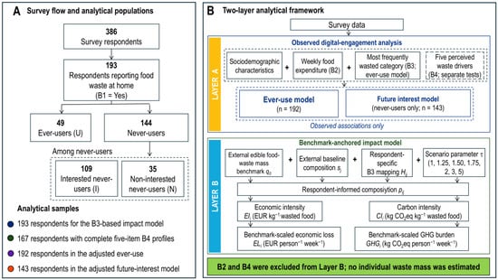
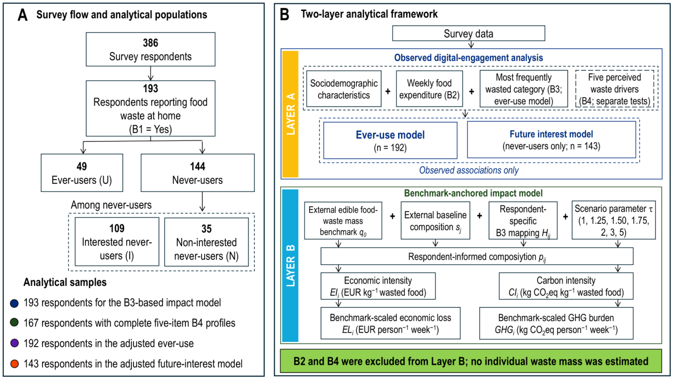
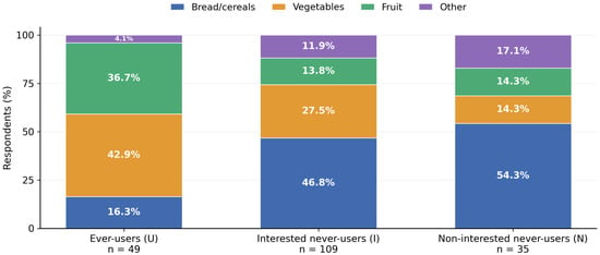
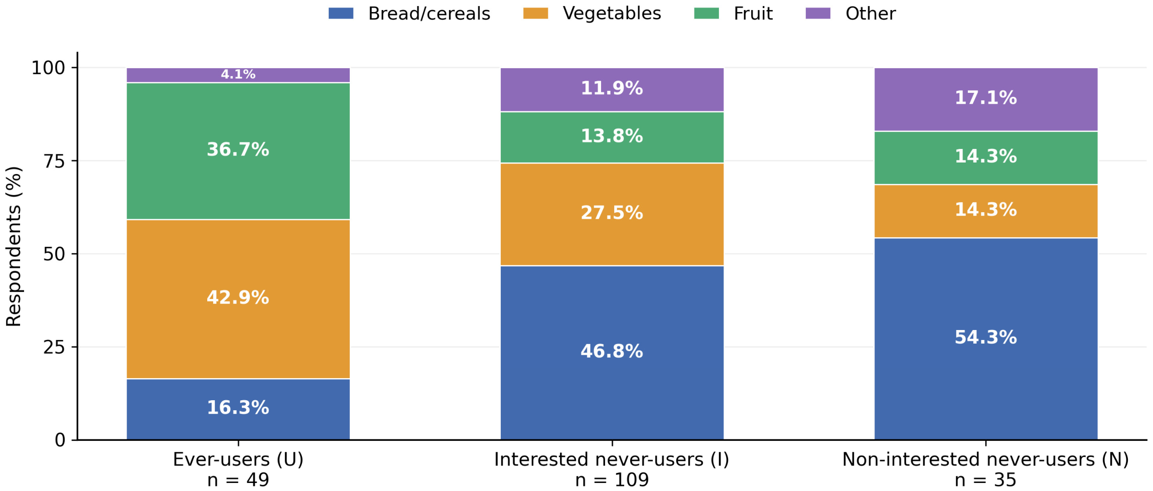
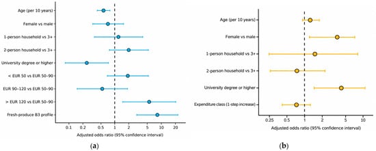
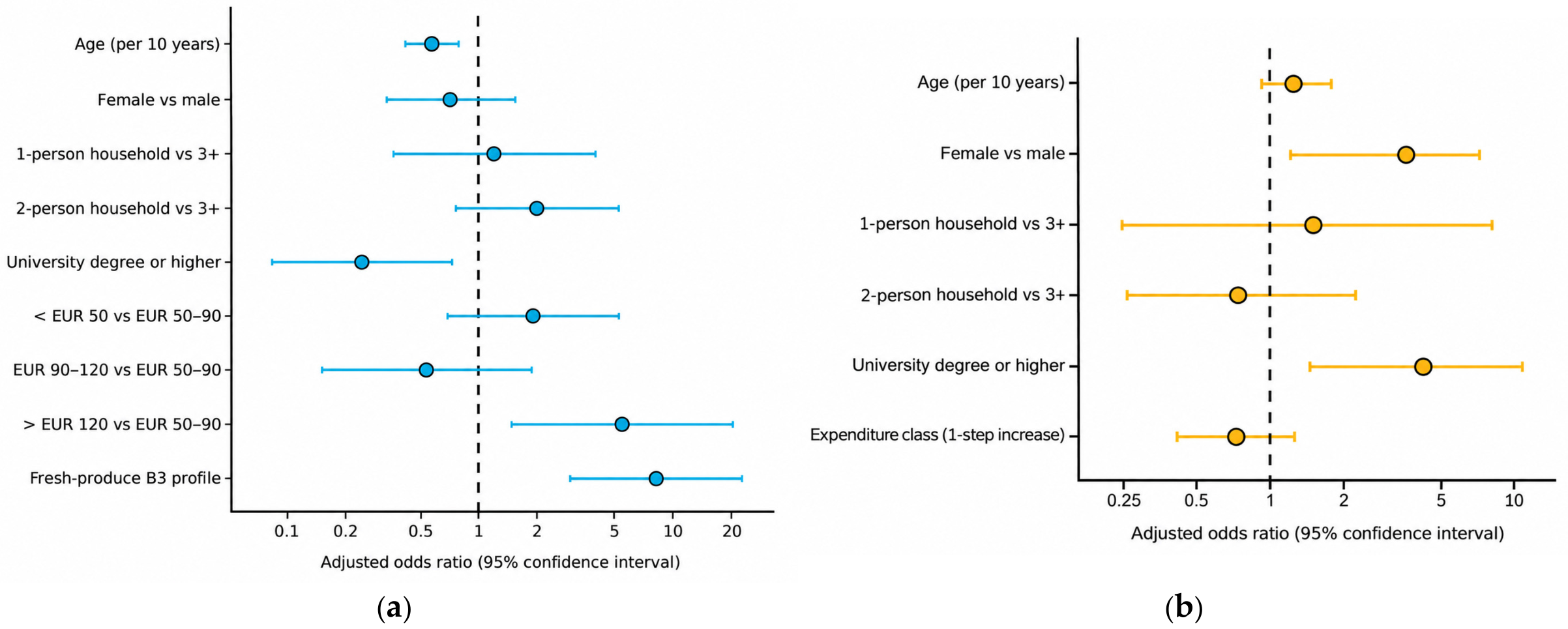
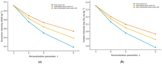
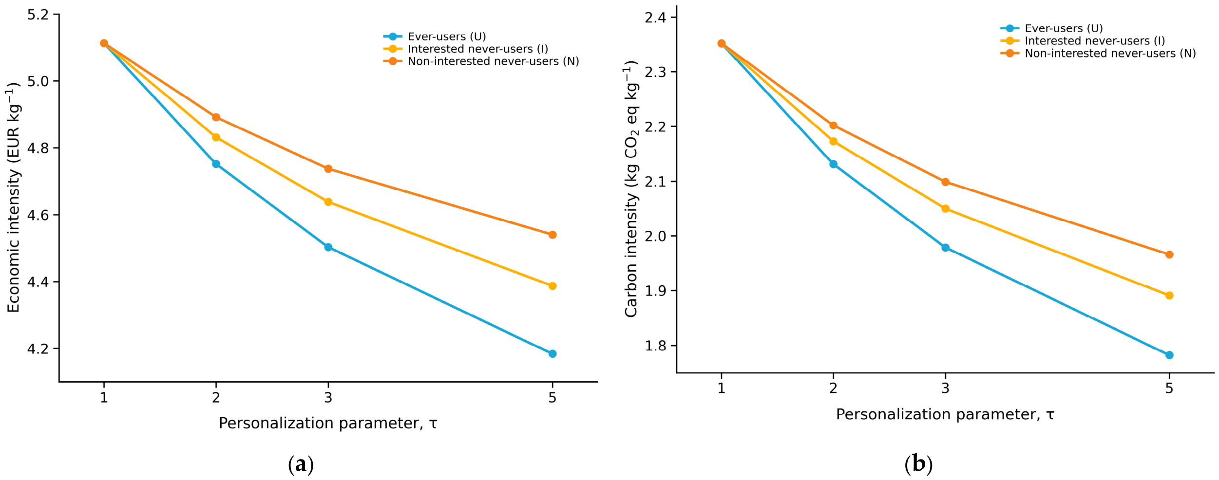
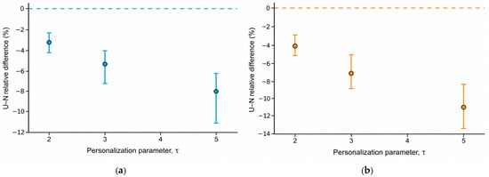
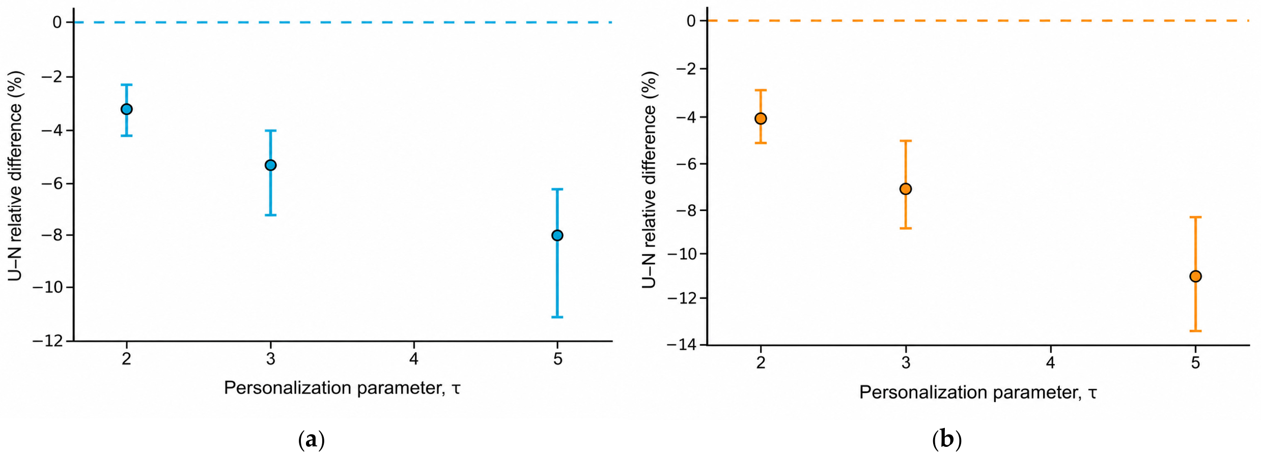

Disclaimer/Publisher’s Note: The statements, opinions and data contained in all publications are solely those of the individual author(s) and contributor(s) and not of MDPI and/or the editor(s). MDPI and/or the editor(s) disclaim responsibility for any injury to people or property resulting from any ideas, methods, instructions or products referred to in the content. |
© 2026 by the authors. Licensee MDPI, Basel, Switzerland. This article is an open access article distributed under the terms and conditions of the Creative Commons Attribution (CC BY) license.