


Abstract
Water quality monitoring is important for protecting aquatic life and supporting informed water quality assessment and environmental decision support. However, many existing systems mainly focus on data collection and threshold-based alerts, without connecting prediction, diagnosis, and intelligent assessment within a unified workflow. This paper proposes an integrated smart aquatic monitoring system using Southeast Texas (SETX) water quality data, advanced machine learning models, large language models (LLMs), and an agentic n8n workflow. Firstly, SETX water quality data are extracted, cleaned, and converted into a structured CSV format. Important water features such as pH, dissolved oxygen, temperature, conductivity, and total dissolved solids are used to train and evaluate four different machine learning models, including Transformer, Quantum Neural Network (QNN), XGBoost, and Random Forest. The ML model is then deployed to a backend system for use inside the n8n automation workflow. For simulation, a Python script is designed to emulate an IoT water quality sensor by reading dataset records, converting valid records into JSON objects, and sending them to an agentic n8n webhook. The n8n workflow receives the sensor data and forwards it to the deployed model to predict surface water quality status. Across three simulations with three different datasets, the ML models demonstrate strong performance in classifying safe and unsafe water conditions. On the SETX dataset, Random Forest achieved the best performance, with 99.97% accuracy and a 99.95% macro F1-score. XGBoost also performed strongly, achieving 99.91% accuracy and a 99.86% macro F1-score. The Transformer model achieved 95.98% accuracy and a 94.00% macro F1-score, while the QNN model achieved 94.78% accuracy and a 92.24% macro F1-score. These results demonstrate that the processed SETX dataset supports reliable water quality prediction and can be integrated into the proposed n8n-based intelligent monitoring workflow. The prediction results are subsequently analyzed by an LLM-based diagnosis agent to generate an LLM-based water quality assessment, risk classification, and assessment summary that explain the prediction and highlight the most influential water quality parameters. The proposed system demonstrates a practical framework for combining sensor simulation, predictive modeling, LLM-based decision support, and agentic workflow automation for intelligent water quality assessment and smart environmental monitoring.
1. Introduction
Dead aquatic organisms and floating debris are usually gathered on the surface of rivers and canals. If these are not removed in time, then they decompose in the water and may reduce oxygen levels and result in higher aquatic life mortality [1]. At the same time, water quality metrics such as pH, dissolved oxygen, turbidity, conductivity, and temperature can fluctuate [2,3], and without proper monitoring, water quality conditions may deteriorate before they are detected [4]. Previous work has focused on these issues separately; however, few studies have integrated intelligent water quality monitoring, machine learning (ML)-based prediction, explainable LLM, and automated workflow orchestration within a single framework.
The main objective of this research is to develop and evaluate an intelligent water quality assessment and decision support framework for SETX surface water monitoring as shown in Figure 1. This study first transforms unstructured SETX water quality PDF reports into a structured dataset suitable for ML analysis. Then, four ML models, including Random Forest, XGBoost, Transformer, and QNN are trained and compared for the classification of surface water as safe or unsafe. This study also uses SHAP analysis to explain the important prediction features and connects the model output with an n8n-based automated workflow for AI-assisted water quality assessment and decision-support summary.
Figure 1.
Intelligent SETX water quality assessment using an n8n workflow.
2. Background and Literature Review
Recent work in intelligent monitoring, robotics-assisted environmental systems, and adaptive sensing shows a clear shift toward integrated, AI-driven environmental frameworks. Advances in bio-inspired robotic mechanisms [5], cable-driven capture systems [6], and occlusion-aware manipulation [7] demonstrate how autonomous platforms are becoming more resilient in uncertain conditions. Real-time sensing continues to improve through distributed imaging accelerators [8] and scale-adaptive detection models [9]. In environmental applications, satellite-based monitoring of sea-ice and iceberg dynamics [10,11] and dynamic watershed-scale water quality diagnosis [12] highlight the growing role of AI in large-scale ecological assessment. Advances in adaptive and event-triggered control [13] further reinforce this movement toward intelligent, autonomous environmental management. Together, these studies help situate the proposed ML–LLM–workflow framework within current trends in intelligent environmental monitoring, explainable AI, and AI-assisted decision support. Table 1 presents a summary of the key studies reviewed in this work. The proposed system integrates IoT sensor data into an agentic n8n workflow, where a transformer model predicts water quality status and large language models generate AI-assisted water quality assessments and decision-support summaries, advancing beyond conventional alerting toward intelligent water quality assessment.
Table 1.
Comparison of existing studies and the proposed work.
3. Research Questions and Hypotheses
Based on Figure 2, this section presents four research questions (RQs) and their corresponding hypotheses.
Figure 2.
Overview of the research questions, hypotheses, workflow, contributions, and expected impacts of the proposed intelligent water quality assessment framework.
RQ1. How can unstructured water quality datasets [32] be converted into structured CSV datasets through a PDF-to-CSV simulation framework to support automated ML-based analysis?
Hypothesis 1.
A Python-based developed software tool can transform unstructured water quality records into structured datasets suitable for ML analysis.
RQ2. What AI-driven workflow framework can be developed to automate water quality assessment and decision support?
Hypothesis 2.
An agentic n8n workflow can automate the execution of ML inference, data processing, and LLM-based water quality assessment by passing outputs sequentially between workflow nodes.
RQ3. Which water quality parameters have the greatest influence on predicting safe and unsafe water conditions?
Hypothesis 3.
Dissolved oxygen, percent saturation, pH, and total dissolved solids will have the greatest influence on water quality classification.
RQ4. Can LLM-generated water quality assessments improve the interpretability of ML predictions for decision support?
Hypothesis 4.
LLM-based reasoning will improve the interpretability of prediction outputs by converting raw sensor measurements and ML predictions into clear water quality assessments and decision-support summaries.
4. Key Contributions
The key contributions are as follows:
- 1.
- The first contribution of this research is the development of a software tool that reads the SETX water quality dataset and prepares it for advanced ML. The PDF dataset from the SETX repository contains missing values, extra columns, invalid data, and different water quality parameters that need to be cleaned and organized before model training. This software tool extracts the required features, such as pH, dissolved oxygen, temperature, conductivity, and total dissolved solids, and converts the data into a structured format suitable for ML models. This allows ML models such as Transformer, QNN, Random Forest, and XGBoost to learn from clean and meaningful water quality data. This contribution is important because accurate predictions depend strongly on the quality of the prepared dataset.
- 2.
- The second contribution is the development of an automated workflow using the agentic n8n platform. After the ML model predicts the water quality, n8n executes the workflow step by step. Each n8n node performs a specific task, such as receiving sensor data, sending the data to the trained model, collecting the prediction result, forwarding the result to the LLM-based assessment node, generating an AI-assisted water quality assessment, determining the risk level, preparing a decision-support summary, and logging the workflow results. This contribution is important because it connects ML prediction with automated workflow execution, enabling the system to provide intelligent water quality assessment and decision support.
- 3.
- The third contribution of this research is the identification of the most important water quality parameters influencing the classification of water as safe or unsafe. This involves analyzing the role of features such as dissolved oxygen, pH, total dissolved solids, segment, percent saturation, temperature, and conductivity in the prediction process. These parameters are important because they directly affect aquatic life and indicate changes in water conditions. By identifying the most influential features, the system becomes more explainable and helps users understand why the model classifies water as safe or unsafe. SHAP analysis is used to determine which water quality features contribute most to the prediction.
- 4.
- The fourth contribution of this research is the use of LLM-based water quality assessment to make ML outputs easier for users to understand and interpret. Instead of presenting raw sensor values or a simple safe/unsafe prediction, the system sends the model prediction and water quality data to an LLM. The LLM explains the predicted water quality condition in clear language, provides an AI-assisted assessment, identifies the corresponding risk level, and generates a decision-support summary. This helps users quickly understand the reason behind the prediction and supports informed decision-making.
In order to conduct the SETX water quality assessment, the official guidelines of the Texas Surface Water Quality Standards (TSWQSs) of the Texas Commission on Environmental Quality (TCEQ), listed below, were followed.
5. Regulatory and Environmental Context
Water quality in the Sabine Pass and Lower Neches River region is influenced by tides, rainfall, storms, and seasonal temperature variations. Because live meteorological observations were not included, temporal variables such as month, day, and hour were incorporated to capture environmental variability affecting dissolved oxygen, salinity, turbidity, and bacterial concentrations.
Target labels were developed using selected criteria inspired by the Texas Surface Water Quality Standards (TSWQSs) established by the Texas Commission on Environmental Quality (TCEQ) [33,34]. Because this study focuses on surface water systems rather than drinking water sources, EPA and WHO drinking water standards were not considered.
The Lower Neches River is divided into two classified segments with different environmental characteristics and regulatory requirements. Segment 0601 represents the tidal region, whereas Segment 0602 represents the freshwater region. Consequently, the segment identifier was included as an input feature so that location-specific criteria could be incorporated into the classification process. Table 2 summarizes the principal criteria considered in this study.
Table 2.
Segment-specific water quality criteria for the Lower Neches River [33].
State reports have identified several environmental concerns in the Lower Neches River, including bacterial contamination, legacy pollutants, and harmful chemicals that may affect aquatic ecosystems [34]. Accordingly, the target feature was generated using selected TSWQs-inspired criteria related to dissolved oxygen, pH, temperature, and total dissolved solids, while temporal and location-specific variables were incorporated to support the classification of safe and unsafe surface water conditions.
6. Proposed Methodology and Approach
The proposed methodology is illustrated in Algorithm 1. The overall workflow is described in the following subsections.
| Algorithm 1 Data extraction, model training, and agentic n8n-based water quality assessment workflow |
|
6.1. Rationale for ML Model Selection
Four ML models are selected. Random Forest is selected as a strong baseline model because it performs well on tabular datasets, effectively captures nonlinear feature interactions, and is generally robust to noisy data. XGBoost is selected because of its strong performance on structured datasets and its ability to handle class imbalance through sample weighting. The Transformer is selected to evaluate whether an attention-based model can effectively learn temporal, station-specific, and physicochemical patterns from the processed SETX records. The QNN is selected as a hybrid quantum–classical model to investigate whether quantum layers can effectively learn water quality patterns and to compare its performance with classical and deep learning models. Together, these four models provide a comprehensive comparison of practical and emerging ML approaches using the same preprocessing, validation, and evaluation framework.
6.2. Data Acquisition and Initial Extraction
The raw data extraction began with the 94 monthly surface water quality PDF reports downloaded from the SETX/Sabine River Authority data repository using a custom lightweight Python script. The original PDF reports contain unstructured water quality data such as paragraphs, figures, tables, charts, and repeated headers. A second automated Python script is developed using the pdfplumber module and custom regular expressions to extract the required water quality data from the tables. This Python script identifies the sampling tables and merges them into a single CSV file, as shown in Figure 3, where each row in the dataset contains the sampling data at a given station and sampling time.
Figure 3.
Development of a software tool for generating a structured SETX water quality dataset.
First, the parser identifies the station header rows and extracts metadata such as sampling date and time, TCEQ station ID, station code, report period, source file, and segment. This metadata is then attached to all associated depth measurements for that station profile. The extraction logic differentiates between valid continuation depth rows and non-measurement text, explicitly filtering out lines produced by chart axes, repeated table headers, USGS flow tables, and other non-observation artifacts.
Missing and non-result values such as NR and NM were kept as empty cells and recorded in the review_flags column for later manual checking. Numeric values, such as temperatures outside the expected physical range, were flagged. Rows missing required physicochemical variables such as pH, dissolved oxygen, conductivity, total dissolved solids, and percent saturation were treated as invalid data and discarded. This approach kept the final extracted dataset close to the original reported measurements.
After the initial extraction, we preprocessed the raw sensor data for ML through the following steps:
- Type Standardization: We converted text-based detection limits (e.g., “<0.1”) into numerical values to ensure that all sensor readings were mathematically compatible.
- Handling Missing Data: We removed columns with high rates of missing values, such as bacteria counts, Secchi depth, and salinity, to improve dataset quality.
- Removing Metadata: We removed administrative fields (e.g., file names, exact timestamps, report_period, source_file, and review_flags) so that the models focused only on the relevant physical measurements.
- Temporal Engineering: We extracted a numerical “month” feature from the date values to capture seasonal variations in the river, while the original date format was discarded.
- Error Filtering: We removed physically invalid sensor readings, such as impossible depth values, to ensure reasonable measurement ranges.
- Mathematical Balancing: We applied a logarithmic transformation (log1p) to the conductivity and TDS columns to reduce right skewness, compress extreme outliers, and improve the data distribution, as shown in Figure 4.Figure 4. Log transformation applied to conductivity and TDS.
6.3. Data Cleaning and Feature Selection
After extracting the water quality data from the PDF reports, the original dataset contained 16,955 rows and 20 columns. During the data-cleaning process, we removed 775 incomplete rows, leaving 16,180 rows and retaining 95.4% of the original data. This indicates that most of the extracted observations were preserved after filtering. To create the ML-ready dataset, we also reduced the number of columns from 20 to 11. The nine removed columns included sparse measurements and non-predictive metadata, while two new temporal features (month and year) were derived from the date field. The final dataset consisted of 16,180 rows and 11 features. Table 3 summarizes the data-cleaning and feature-preparation steps.
Table 3.
Summary of data cleaning and feature preparation.
The feature-selection process is based on data quality, environmental relevance, and model explainability. The selection is guided by the following criteria: (1) Columns with high rates of missing values or limited predictive usefulness are removed, including sparse bacteria-related fields, Secchi depth, file names, timestamps, and review flags. (2) Features directly related to the TSWQs-guided safe/unsafe surface water labels are retained, including pH, dissolved oxygen, temperature, conductivity, total dissolved solids, and percent saturation. (3) Temporal and location-related features representing seasonal and spatial variations in the SETX monitoring region are retained, including month, year, segment, and station ID. Table 4 summarizes the final input features used for surface water status classification. After data cleaning and feature selection, all four ML models are trained, SHAP analysis is performed, and the resulting feature-importance analysis was used to identify the variables that contributed most to the predictions. Therefore, feature selection was not based solely on model accuracy but also considered data quality, regulatory relevance, and model explainability.
Table 4.
Final input features used for surface water status classification.
Regulation-Guided Target Label Generation
In the final dataset, the target column represents the regulation-guided surface water status rather than drinking-water potability. Each record is evaluated using physicochemical criteria derived from the TSWQSs. These rules established threshold limits for pH, dissolved oxygen, temperature, and total dissolved solids (TDS), as shown in Table 5. Because environmental baselines differ by water type, the labeling logic applied different threshold conditions for freshwater and tidal river segments. Samples satisfying all applicable thresholds are labeled as safe (Class 0), whereas those violating one or more criteria were labeled as unsafe (Class 1). This binary rule-based label served as the target variable for all machine learning models used in this study.
Table 5.
Considered rule-based criteria used for water status labeling, inspired by TSWQs guidelines.
Table 6 shows the class distribution in the dataset, where 78.23% of the samples are labeled as safe and 21.77% as unsafe. To ensure that this class imbalance did not bias model evaluation, we applied StratifiedKFold across all data splits so that the 78:22 class ratio was approximately preserved in the training, validation, and test sets. In addition, Random Forest and XGBoost are trained using balanced class weighting to reduce majority-class bias during learning. Finally, we report accuracy, macro F1-score, and the Matthews Correlation Coefficient (MCC), as these metrics provide a balanced evaluation of model performance, particularly for the minority “unsafe” class.
Table 6.
Class distribution of the final ML-ready dataset.
To avoid data leakage, the scaler and encoder were fitted only on the training data. The validation and test sets are transformed using the fitted scaler and encoder obtained from the training data and were not used during the fitting process.
6.4. Class Imbalance and Unsafe-Class Performance
Because the dataset is imbalanced (78.2% safe and 21.8% unsafe), model performance was evaluated based on the detection of unsafe samples. Table 7 reports the per-class recall, unsafe-class F1-score, and MCC, and Figure 5 shows the corresponding confusion matrices on the held-out test set (3236 samples: 2531 safe and 705 unsafe). The best-performing value in each evaluation metric is shown in bold.
Table 7.
Per-class recall and MCC on the test set, emphasizing minority (unsafe) detection.
Figure 5.
Confusion matrices for the four models on the held-out SETX test set. (a) Random Forest. (b) XGBoost. (c) Transformer. (d) QNN.
These results show that, despite the class imbalance, all four ML models achieved high unsafe-class recall, with the tree-based models in particular missing very few unsafe samples. The strong MCC values (0.9991 for Random Forest and 0.9973 for XGBoost) confirm that the observed performance is not simply an artifact of majority-class dominance, since MCC is only high when both classes are classified accurately.
6.5. Docker Environment
To host the n8n workflow on the local machine, we used Docker. We pulled the n8n image and ran it inside a Docker container. The container publishes port 5678, so the n8n editor is reachable at http://localhost:5678/, where we built our workflow. Docker also allows the container to send HTTP requests to services running outside the Docker environment. In our setup, we hosted the ML model on the local system and ran a second Python script that mimics a water quality IoT sensor. Both services are accessible from the n8n nodes running inside the container.
6.6. Sensor Data Simulation and n8n Workflow Execution: Webhook Node as a Trigger
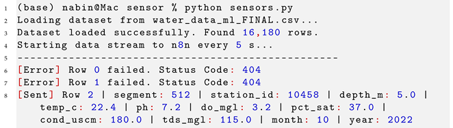
To emulate a real-time water quality monitoring system and IoT sensor, we developed a Python script (sensor.py). The script reads the test dataset record by record to validate and remove incomplete and out of range sensor entries. The workflow starts with a Webhook node, which receives the simulated water-quality sensor data directly in JSON format and forwards it to the backend machine-learning model for prediction. A delay of 5 s between consecutive requests was introduced to simulate continuous sensor measurements. Listing 1 presents an example of the sensor simulator output in terminal.
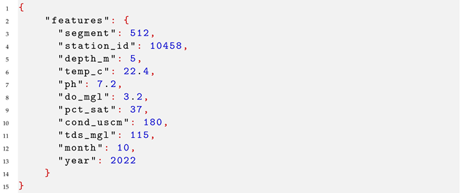
The webhook node receive data in JSON format as in Listing 2 and transmitted to the next node which performs machine-learning-based prediction.
| Listing 1. Each valid record is converted into JSON format and transmitted to the n8n workflow. |
 |
| Listing 2. Water quality record transmitted to the n8n webhook. |
 |
6.7. Backend Services for SETX Water Quality Safe and Unsafe Predictions Using Transformer, QNN, XGBoost, and Random Forest
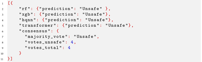
All water-quality features received by the Webhook node in JSON format are passed to an HTTP Request node, which sends each record to the backend service for prediction. The backend hosts four pretrained models, namely Random Forest, XGBoost, Transformer [35], and QNN [36], and applies all four models to each incoming record to predict the surface-water status. Each model independently classifies the status as Safe or Unsafe. After inference, the backend returns the individual model predictions and consensus result in JSON format to the n8n workflow, as shown in Listing 3. The response is then parsed automatically and forwarded, together with the original sensor record, to the subsequent LLM-based water-quality assessment node.
| Listing 3. Model prediction results. |
 |
6.8. Proposed Agentic n8n Workflow for SETX Water Quality Assessment
The proposed system is implemented on the n8n: AI Workflow Automation Platform that combines several automated steps (Table 8). The workflow (Figure 6) starts with a Webhook node, which triggered after receiving data record from a simulated Python script based IoT water quality sensor and passes them to the HTTP node for prediction as discussed in Section 6.6 and Section 6.7. This n8n webhook node serves as the data-ingestion component of the workflow.
Table 8.
Node-to-node data flow in the proposed workflow.
Figure 6.
n8n workflow for AI-assisted SETX water quality assessment and decision support.
First node in the workflow Figure 6 is Webhook trigger (lightning-bolt icon) from where workflow begins. Solid arrows shows the sequential data flow between nodes. The dashed lines labeled “Model” denote the attachment of the underlying OpenAI chat model to each LLM agent node. The red asterisk (*) on the “Chat Model” indicates a required model connection. The workflow ends with three open branches. These nodes can be extended to add further features, such as supervisor alerts and human-in-the-loop review, toward a fully autonomous water monitoring system.
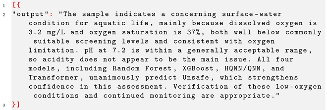
After getting model prediction as shown in Listing 3 then it is passed along with the sensor data readings (record) to LLM1 Assessment, which analyzes the model output and water quality features to generate an AI-assisted water quality assessment as shown in the Listing 4.
| Listing 4. LLM1 Assessment response. |
 |
Next, LLM1 assessment is pass to LLM2 Decision Support Node to determine the corresponding risk level and generate a decision-support summary as shown in the Listing 5.
| Listing 5. LLM2 Decision Support response. |
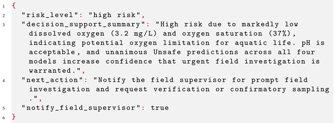 |
Finally, the workflow follows the appropriate branch based on the predicted risk level, generating the corresponding decision-support summary for subsequent review and decision making.
LLM Output Validation and Reliability
The proposed framework incorporates two LLM agents as interpretation and decision-support components rather than autonomous decision-making systems.
LLM1 generates an AI-assisted water quality assessment by interpreting the predicted water quality status. The assessment identifies the key water quality parameters contributing to the prediction, explains why they indicate either safe or unsafe conditions, and summarizes their potential ecological impacts on aquatic life. This process transforms numerical ML outputs into an interpretable assessment that assists domain experts in understanding the predicted water quality condition.
The AI-assisted assessment generated by LLM1 (Open AI GPT model) is then forwarded to the second LLM2. Using the assessment from LLM1, LLM2 determines the corresponding water risk level and generates a concise decision-support summary. The ML models remain the primary source of the safe or unsafe prediction, while the two LLM agents enhance the interpretability of the prediction and provide contextual decision support without replacing the underlying machine learning models or the predefined regulatory criteria.
This two-stage LLM architecture improves the interpretability of the prediction workflow by combining quantitative machine learning predictions with qualitative natural language explanations. Consequently, domain experts can more easily understand the factors influencing the prediction, evaluate the associated environmental risks, and support timely decision making for surface water quality monitoring. Table 9 summarizes the corresponding workflow actions.
Table 9.
Risk classification criteria and corresponding workflow actions.
7. Simulation Results and Discussion Using the SETX Dataset
The flowchart of the proposed framework is shown in Figure 7. The system classifies the surface water quality status using four machine learning models: Random Forest, XGBoost, Transformer, and QNN. All models were evaluated on the processed SETX dataset using safe/unsafe water quality labels inspired by the TSWQs framework. The final dataset contained 16,180 observations with 11 input features.
Figure 7.
Flowchart of the proposed water quality assessment framework.
7.1. Dataset Description
All four ML models evaluated in this experiment are trained using the same SETX dataset described in Section 6.2. The final dataset contained 16,180 samples with 11 input features, including seven numerical features (depth, temperature, pH, dissolved oxygen, percent saturation, conductivity, and total dissolved solids), two categorical features (segment and station ID), and two temporal features (month and year). The class distribution consisted of 12,657 safe samples (78.23%) and 3523 unsafe samples (21.77%).
The dataset is divided into 80% for model development and 20% for the held-out test set using stratified sampling to preserve the safe/unsafe class distribution in both subsets. A fixed random seed (random_state=42) was used to ensure reproducibility. Samples containing missing required measurements had already been removed during the data cleaning stage (Section 6.2). During pre-processing, numerical features are scaled and categorical features RE ordinally encoded. These pre-processing steps were fitted only on the training data and then applied to the held-out test data to prevent information leakage.
7.2. XGBoost
XGBoost is a gradient-boosting algorithm that sequentially constructs decision trees, with each new tree learning to correct the errors made by the previous trees. The model used 200 trees with a maximum tree depth of 6 and a learning rate of 0.1. To address the class imbalance, the scale_pos_weight parameter was set to approximately 3.59, corresponding to the ratio of safe to unsafe samples. Row and column subsampling (both set to 0.8) were also used to reduce overfitting. The model was trained using the binary:logistic objective function with log-loss as the evaluation metric.
On the held-out test set, XGBoost achieved an accuracy of 99.91%, a macro F1-score of 99.86%, and a ROC–AUC of 1.0000. For the unsafe class, the model achieved a precision of 99.86%, a recall of 99.72%, and an MCC of 0.9973. These results indicate that XGBoost learned the TSWQS-based rule-derived labels with very high accuracy. According to the model’s feature importance analysis, dissolved oxygen, pH, and total dissolved solids were the most influential features, which is consistent with the parameters used to generate the TSWQS-based labels.
7.3. Random Forest
Random Forest is an ensemble learning algorithm that constructs multiple decision trees using random subsets of the training data and combines their predictions through majority voting. The model used 200 decision trees with no maximum depth restriction, and each split considered a random subset of the available features (max_features=sqrt). To address class imbalance, the class_weight parameter was set to balanced, giving greater importance to the minority unsafe class. A fixed random seed of 42 was used throughout training.
On the held-out test set, the Random Forest model achieved the strongest overall performance, with an accuracy of 99.97%, a macro F1-score of 99.95%, and a ROC–AUC of 1.0000. For the unsafe class, it achieved 100% precision and 99.86% recall, misclassifying only one of the 705 unsafe samples in the test set. The model also achieved the highest MCC (0.9991) among all four evaluated models. The feature importance analysis identified dissolved oxygen, percent saturation, and pH as the most influential variables, which is consistent with the physicochemical parameters used to generate the TSWQS-based labels.
7.4. Transformer Model
The Transformer model applies the attention mechanism, originally developed for natural language processing, to structured tabular data. This architecture can learn relationships among input features rather than processing each feature independently.
The model used an embedding dimension of 32, four attention heads, and two Transformer encoder layers, with a feed-forward hidden dimension of 16 and a dropout rate of 0.1. The two categorical features (segment and station ID) together with the two temporal features (month and year) were represented as categorical variables and converted into learned embeddings, resulting in four embedded inputs. A CLS token is used to aggregate the learned feature representations before the final binary classification layer. The model was trained for 15 epochs using the Adam optimizer (learning rate = 0.001), a batch size of 128, and the BCEWithLogitsLoss loss function.
On the held-out test set, the Transformer achieved an accuracy of 95.98%, a macro F1-score of 94.00%, and a ROC–AUC of 0.9909. For the unsafe class, the model achieved a recall of 88.37%, indicating that it correctly identified most unsafe samples but misclassified more unsafe samples than the two tree-based models. This behavior is commonly observed for deep learning models applied to structured tabular datasets, where larger training datasets are often required to match the performance of gradient-boosting and Random Forest models.
7.5. QNN
The QNN combines a small classical neural network with a quantum circuit. The model is implemented using PennyLane (Version 2.10) and PyTorch (Version 2.8.0) on the default.qubit simulator. First, a classical layer compressed the input features—the seven numerical features together with the two categorical and two temporal features (represented as four embedded categorical inputs)—into four latent values. These four values were then encoded into a four-qubit quantum circuit using AngleEmbedding, followed by two StronglyEntanglingLayers, which formed the trainable quantum component. The circuit outputs are obtained using Pauli-Z expectation values, and a final classical layer generated the binary classification output.
Because quantum circuit simulation is computationally expensive, the final QNN model was trained using a stratified subset of 1500 samples for 10 epochs with the Adam optimizer (learning rate = 0.01) and a batch size of 64. The trained model is subsequently evaluated using the complete held-out test set. On the test set, the QNN achieved an accuracy of 94.78%, a macro F1-score of 92.24%, and a ROC–AUC of 0.9773. For the unsafe-water class, the model achieved a recall of 86.24%. Although the QNN is trained using only a small subset of the available training data and employed only four qubits, the results demonstrate that hybrid quantum neural networks have promising potential for water quality classification.
7.6. Comparative Analysis
Table 10 compares the performance of the four ML models on the held-out test set. The two tree-based models, Random Forest and XGBoost, achieved the strongest overall performance, with near-perfect results across all evaluation metrics and only a small number of misclassified unsafe-water samples. The Transformer and QNN also demonstrated strong predictive performance but produced slightly lower scores, primarily because they misclassified a larger number of unsafe-water samples. Because the TSWQS-based labels were generated directly from threshold rules applied to the same physicochemical water quality parameters used as model inputs, it is expected that sufficiently expressive machine learning models can closely approximate these decision boundaries. This observation is discussed further in the validation and data leakage analysis presented in Section 6.2.
Table 10.
Comparison of model performance on the SETX surface water quality classification task (80/20 stratified split using TSWQS-based labels).
7.7. Cross-Validation Results
Five-fold stratified cross-validation was performed on the 80% development set before the final evaluation on the held-out test set, as summarized in Table 11. This evaluation was conducted to assess model stability and reduce dependence on a single training–test split. Across the five folds, the Random Forest and XGBoost models demonstrated the most consistent performance, with mean MCC values greater than 0.996. The Transformer and QNN also achieved strong cross-validation performance, with mean ROC–AUC values of 0.9888 and 0.9858, respectively.
Table 11.
Five-fold stratified cross-validation results on the 80% development set.
8. Split-Based Analysis
8.1. Evaluation Protocol for the 80/20 Split
In the primary experiment, the four ML models are trained and evaluated using an 80/20 training–test split of the final SETX dataset. The training files, X_train.csv and y_train.csv, contained 12,944 samples, whereas the held-out test files, X_test.csv and y_test.csv, contained 3236 samples. Five-fold stratified cross-validation was performed only on the training portion of the dataset. The held-out test set remained completely separate and is used exclusively for the final model evaluation. This evaluation protocol minimized the risk of data leakage; however, it assessed model performance under only a single training–test split ratio.
8.2. Dataset Used for Split Analysis
The split-ratio analysis used the same final SETX dataset as the primary experiment. The target labels are reconstructed by combining y_train.csv and y_test.csv. No additional samples or features were introduced, and no existing samples are removed. The TSWQS-based safe/unsafe labels are generated before feature scaling and encoding. Subsequently, the log1p transformation is applied to the right-skewed conductivity and total dissolved solids (TDS) features before model training. For every training–test split, feature scalers and categorical encoders are fitted using only the training data to prevent data leakage.
8.3. Additional Training–Test Split Ratios
To further evaluate model robustness and generalizability, the original experiment was repeated using three additional training–test split ratios: 90/10, 70/30, and 60/40. The 90/10 split allocated a larger proportion of the data for model training, the 70/30 split provided a balanced trade-off between training and evaluation, and the 60/40 split reduced the amount of training data to assess whether the models could maintain good generalization with fewer training samples.
For each split ratio, stratified sampling with random_state=42 is used to preserve the safe/unsafe class distribution in both the training and test sets. Five-fold stratified cross-validation is then performed using only the training portion of the data. After cross-validation, each model was retrained using the complete training subset and evaluated once on the corresponding held-out test set. Because of the computational cost associated with quantum circuit simulation, the QNN was trained using a stratified subset of 2000 samples from the training data while maintaining the original class distribution.
8.4. Results Across Split Ratios
Table 12 summarizes the held-out test performance of the four ML models using three additional training–test split ratios.
Table 12.
Held-out test results for the four ML models across different training–test split ratios.
The results demonstrate that the Random Forest and XGBoost models remained highly stable across all training–test split ratios. Both models achieved ROC–AUC values of approximately 1.0000, while their MCC values remained above 0.995, indicating that the tree-based models were largely insensitive to variations in the amount of training data.
The Transformer also exhibited stable performance across the different split ratios. Its ROC–AUC ranged from 0.9891 to 0.9932, while the MCC ranged from 0.8801 to 0.8988. These results indicate that the Transformer consistently learned the TSWQS-based safe/unsafe classification patterns despite changes in the proportion of training data.
The QNN exhibited greater variability across the different split ratios. It performed well under the 70/30 and 60/40 splits, achieving ROC–AUC values of 0.9860 and 0.9810, respectively. However, its performance under the 90/10 split was substantially lower, with an accuracy of 0.7824, a ROC–AUC of 0.5000, and an MCC of 0.0000. These results indicate that the model converged to a majority-class prediction during the final evaluation, even though the cross-validation folds obtained during training produced strong validation ROC–AUC values.
Overall, the split-ratio analysis leads to three main observations. First, the Random Forest and XGBoost models are the most robust across all evaluated training–test splits, maintaining consistently high predictive performance. Second, the Transformer also demonstrated stable performance, although its accuracy and MCC are slightly lower than those of the tree-based models. Third, the QNN is the most sensitive to changes in the training–test split, performing well under the 70/30 and 60/40 configurations but exhibiting optimization collapse during the final evaluation under the 90/10 split.
8.5. Ablation and Hyperparameter Sensitivity Analyses
To further evaluate model robustness, an ablation study is conducted to investigate how each model responded to changes in its primary hyperparameters. For every simulation, the same SETX dataset and the TSWQS-based safe/unsafe labels are used, and the ROC–AUC was recorded as the evaluation metric. The investigated hyperparameters included the number of trees and maximum tree depth for the Random Forest model; maximum tree depth, learning rate, and number of estimators for XGBoost; the number of attention heads, encoder layers, and dropout rate for the Transformer; and the number of qubits and quantum layers for the QNN. The results are summarized in Table 13, Table 14, Table 15 and Table 16.
Table 13.
Random Forest ablation: ROC–AUC across tree count and maximum depth.
Table 14.
XGBoost ablation: ROC–AUC across maximum depth, learning rate, and number of estimators.
Table 15.
Transformer ablation: ROC–AUC across the number of attention heads, encoder layers, and dropout rate.
Table 16.
QNN ablation: ROC–AUC across the number of qubits and quantum layers.
The results show that the Random Forest and XGBoost models remained highly consistent across all evaluated hyperparameter settings, with ROC–AUC values close to 1.000. These results should be interpreted in the context of the TSWQS-based rule-derived labels. Because the safe/unsafe labels are generated using threshold-based rules applied to physicochemical water quality parameters, tree-based models can effectively learn these threshold boundaries. Consequently, the ablation results primarily demonstrate the stability of the models for this rule-based classification task rather than independent validation of regulatory compliance.
In contrast, the Transformer and QNN models are more sensitive to architectural changes. The Transformer achieved its best performance using four attention heads and two encoder layers, producing a ROC–AUC of 0.9880. The QNN improved from a ROC–AUC of 0.9231 with two qubits to 0.9750 with four qubits, while increasing the number of quantum layers from two to three did not produce further improvement. Overall, the results indicate that none of the evaluated models depend critically on a single hyperparameter configuration, demonstrating stable performance across a reasonable range of model settings.
8.6. Noise Sensitivity Analysis
To further evaluate model robustness, synthetic sensor-like noise is added to all continuous water quality variables, including depth, temperature, pH, dissolved oxygen, percent saturation, conductivity, and total dissolved solids (TDS). Categorical and temporal variables, including segment, station ID, month, and year, were not modified. The safe/unsafe target label is also kept unchanged. Noise levels of 0%, 1%, 3%, 5%, and 10% were evaluated using the same training–test split for each experiment.
Table 17 summarizes the performance of the four models under increasing levels of synthetic sensor noise. As expected, model performance gradually decreased as the noise level increased. Random Forest and XGBoost demonstrated excellent baseline performance and remained highly robust under moderate noise conditions. At the 10% noise level, XGBoost maintained an accuracy of 95.24%, a ROC–AUC of 0.9875, and an MCC of 0.8605. Similarly, the Random Forest model maintained an accuracy of 94.31% and a ROC–AUC of 0.9845. The Transformer demonstrated the strongest robustness under noisy input, achieving the best overall performance at the 10% noise level, with an accuracy of 96.20%, a ROC–AUC of 0.9902, and an MCC of 0.8905. Although the QNN is more sensitive to increasing noise levels, it still maintained a ROC–AUC of 0.9304 at the 10% noise level. Overall, these results demonstrate that the Random Forest, XGBoost, and Transformer models remain robust under moderate sensor-like input disturbances, supporting their suitability for practical water quality monitoring applications.
Table 17.
Noise sensitivity results.
8.7. Deployment Cost and Scalability
Runtime performance is evaluated to determine whether the proposed ML models are suitable for deployment within the proposed n8n-based decision-support workflow. Among the four models, Random Forest and XGBoost exhibited the lowest computational cost because they can be executed efficiently on standard CPU hardware while requiring relatively small model sizes. These characteristics make them well suited for real-time surface water quality assessment within the proposed workflow.
The Transformer and QNN models require greater computational resources than the tree-based models. The Transformer employs deep neural network layers and feature embeddings, whereas the QNN relies on quantum circuit simulation, which is computationally more expensive when executed on conventional CPU hardware. Consequently, although these models provide valuable benchmarks for comparative analysis and future research, they are currently less practical than Random Forest and XGBoost for real-time deployment in operational monitoring systems.
8.8. SHAP Analysis
After training and evaluating the four ML models, SHAP (SHapley Additive exPlanations) analysis is performed to identify the features that each model relied upon when making predictions. This analysis is important because high predictive accuracy alone does not guarantee that a model has learned meaningful physicochemical relationships. The TSWQS-based water quality labels used in this study are primarily determined by dissolved oxygen, pH, temperature, and total dissolved solids (TDS). Therefore, SHAP analysis enables us to determine whether each model follows these regulatory criteria directly or instead relies on correlated features as proxy variables. SHAP values were computed using the held-out test set so that the resulting explanations reflect model behavior on previously unseen data.
8.8.1. Random Forest
The Random Forest SHAP results shown in Figure 8 provide a clear feature ranking, with dissolved oxygen (do_mgl) identified as the most influential feature. It has a mean value of approximately 0.22, which is more than twice that of pH. Other important features include pH, percent saturation, TDS, and conductivity (cond_uscm), whereas variables such as station_id and other administrative features contribute substantially less to the model predictions. This feature ranking is consistent with the Texas Surface Water Quality Standards (TSWQS), which are primarily based on these physicochemical water quality parameters.
Figure 8.
(a) SHAP global feature importance for the Random Forest model. (b) SHAP summary.
The SHAP beeswarm plot in Figure 8b illustrates the direction of each feature’s contribution to the model predictions. Low dissolved oxygen values (blue points) shift predictions toward the unsafe water class, which is consistent with established aquatic environmental principles. The pH feature exhibits a bipolar pattern, where both low and high pH values increase the likelihood of predicting the unsafe class, reflecting the acceptable regulatory pH range defined by the TSWQS. Similarly, higher TDS values shift predictions toward the unsafe class, indicating their influence on water quality classification.
8.8.2. XGBoost
XGBoost produced results similar to those of the Random Forest model, with higher raw SHAP magnitudes because the XGBoost outputs are expressed as log-odds rather than probabilities. In Figure 9a, dissolved oxygen has the highest mean value of 3.56, followed by pH (2.43) and TDS (1.74). Percent saturation, segment, temperature, and conductivity form a clear secondary group, whereas the temporal features (month and year) and depth have the lowest SHAP values. The beeswarm plot in Figure 9b further confirms the physically meaningful relationships, where low dissolved oxygen shifts the prediction toward the unsafe class. The bipolar effect of pH is also evident, and high TDS values shift predictions toward the unsafe class. The relatively low SHAP values for the temporal and station-related features indicate that the model does not rely heavily on the sampling calendar or station identity for prediction.
Figure 9.
(a) SHAP global feature importance for XGBoost. (b) SHAP summary.
8.8.3. QNN
The feature ranking for the QNN is shown in Figure 10a, where dissolved oxygen is identified as the most important feature by a wide margin, with a mean value of 0.14. Dissolved oxygen strongly dominates the feature ranking, with an importance value more than three times greater than those of the next most influential features, pH and segment (both approximately 0.04), followed by TDS, percent saturation, and the remaining variables.
Figure 10.
(a) SHAP global feature importance for QNN. (b) SHAP summary.
The beeswarm plot in Figure 10b shows patterns similar to those observed for the tree-based models. Low dissolved oxygen shifts predictions toward the unsafe class, and high TDS values produce the same effect. The bipolar effect of pH is also visible but is less pronounced than that observed for the Random Forest and XGBoost models. The model compresses all 11 input features into four latent values before they enter the four-qubit circuit, forcing the network to be selective about which information is retained. Using four latent channels, the model preserves the strongest direct signals, such as dissolved oxygen and pH, while allowing weaker or highly correlated features to contribute less. This architectural bottleneck effectively acts as an implicit feature selection mechanism.
8.8.4. Transformer
The Transformer SHAP analysis differs from those of the other three models. In the initial Transformer model, which achieved a test accuracy of 95.98%, the SHAP analysis shown in Figure 11a ranked month as the most influential feature, followed by dissolved oxygen and pH. Although dissolved oxygen and pH remained among the three most important features, the month variable appeared as the single most influential predictor. The beeswarm plot in Figure 11b shows a consistent pattern, with month contributing the largest SHAP values.
Figure 11.
(a) SHAP global feature importance for the Transformer model. (b) SHAP summary.
These results suggest that the Transformer uses month as a seasonal proxy for the same hypoxia-related patterns that the other models learn directly from dissolved oxygen. Months associated with low summer dissolved oxygen concentrations are closely correlated with unsafe water samples in the SETX dataset, making month a strong predictor even though it is not a direct physicochemical water quality parameter.
To determine whether this SHAP result was caused by limited model capacity or insufficient training, the Transformer was retrained using a higher-capacity architecture and a longer training schedule. Specifically, d_model was increased from 32 to 64, the number of encoder layers was increased from 2 to 3, the dropout rate was increased from 0.1 to 0.2, cosine learning-rate decay was adopted, and early stopping based on the validation MCC was applied. The revised model achieved a higher test accuracy of 96.88%, an improved MCC of 0.91, and a higher unsafe-water recall (90.9% versus 88.4%). However, the SHAP analysis of the improved model produced nearly identical feature rankings, with month remaining the most influential feature, followed by dissolved oxygen and pH. These results indicate that, in addition to physicochemical measurements, the Transformer captures seasonal context through the month feature. In this dataset, month likely reflects seasonal variations in temperature, dissolved oxygen, rainfall, runoff, and river conditions. Therefore, the Transformer SHAP results suggest that the model learns meaningful seasonal context in addition to direct physicochemical water quality characteristics.
To further evaluate the robustness and generalizability of the proposed framework, simulations 2 and 3 were conducted using additional water quality datasets collected from different sources and environmental conditions.
8.9. Simulation 2: External Dataset
8.9.1. Dataset Description
This experiment used a large-scale water quality dataset containing 1,048,575 samples and 24 features. The dataset includes numerous physicochemical water quality parameters, including pH, iron, nitrate, chloride, lead, zinc, turbidity, fluoride, chlorine, manganese, and color. These parameters directly influence aquatic ecosystem health and the survival of aquatic organisms. Because the dataset contains common water quality indicators as well as heavy metal concentrations, it is well suited for water safety classification in environmental monitoring applications. Before model training, the dataset was preprocessed to handle missing values and prepare the features for machine learning.
8.9.2. ML Model 1: Transformer-Based Water Quality Classifier
A Transformer-based classification model was trained and evaluated using this dataset. The model employed an optimal decision threshold of 0.39, determined through threshold tuning to improve classification performance for both classes. Using this threshold, the model achieved an overall accuracy of 86.71% on a test set containing 20,000 samples.
8.9.3. ML Model 2: QNN
The QNN model was implemented using the PyTorch framework and trained on a subset of 10,000 samples from the same dataset. The model was initialized with 17 normalized input features and trained on a CPU for 200 epochs. The training loss was monitored every 20 epochs to evaluate convergence. The loss decreased from 0.7570 at Epoch 20 to 0.4463 at Epoch 200, demonstrating that the QNN successfully learned meaningful patterns from the water quality data. The model achieved an overall accuracy of 82.95% on a test set containing 2000 samples.
8.9.4. ML Model 3: Random Forest Classifier
A Random Forest classifier was trained using the same dataset. The model consisted of 300 decision trees with a maximum tree depth of 20, and each split considered a random subset of the available features. During preprocessing, missing numerical values were replaced with median values, whereas missing categorical values (color, source, and month) were replaced with the most frequent category. After training on 734,001 samples and evaluating on a test set of 157,287 samples, the model achieved an accuracy of 87.04% and a ROC–AUC of 92.16%. SHAP analysis identified manganese, pH, turbidity, and chloride as the most influential features for prediction.
8.9.5. ML Model 4: XGBoost Classifier
The XGBoost model was configured with 400 trees, a maximum tree depth of 6, and a learning rate of 0.05. To reduce overfitting, both row and column subsampling rates were set to 0.8. To address class imbalance, the scale_pos_weight parameter was set to approximately 3.36, corresponding to the ratio of safe to unsafe samples in the training data. Using the same test set of 157,287 samples, the model achieved an accuracy of 87.02% and a ROC–AUC of 91.78%, producing performance comparable to that of the Random Forest model. SHAP analysis showed that manganese, color, pH, turbidity, and chloride were the most influential features.
8.9.6. Comparative Analysis
Table 18 compares the performance of the four machine learning models evaluated in simulation 2.
Table 18.
Performance comparison of the four machine learning models evaluated in simulation 2.
The results indicate that the Random Forest model achieved the highest overall accuracy (87.04%), closely followed by XGBoost (87.02%) and the Transformer model (86.71%). Although the QNN achieved a lower accuracy of 82.95%, it demonstrated competitive performance despite being trained on only 10,000 samples because of computational limitations, whereas the other models were trained using substantially larger datasets. Overall, the results demonstrate that the proposed machine learning framework can effectively classify safe and unsafe water conditions using multi-parameter water quality measurements, providing a solid foundation for integration into the proposed n8n-based intelligent monitoring framework.
8.10. Simulation 3: External Dataset
8.10.1. Dataset Description
Experiment 3 used a water quality dataset consisting of chemical and biological parameters. The dataset contains 7999 samples and 21 features, including aluminium, arsenic, barium, cadmium, chloramine, chromium, copper, fluoride, bacteria, viruses, lead, nitrates, nitrites, mercury, perchlorate, radium, selenium, silver, and uranium. Unlike the SETX dataset, this dataset does not include general water quality parameters such as pH, dissolved oxygen (DO), or turbidity. Therefore, this experiment focused on contaminant-based water safety classification rather than comprehensive surface water quality assessment.
8.10.2. ML Model 1: Random Forest Classifier
A Random Forest classifier was trained and evaluated using this dataset. A test set of 2834 samples was used for model evaluation. The Random Forest model achieved an accuracy of 97.38%, with precision, recall, and F1-score values of 0.97, demonstrating excellent classification performance. However, its performance was slightly lower than that of the Transformer model, which achieved the highest accuracy of 97.49%.
8.10.3. ML Model 2: XGBoost Classifier
The XGBoost model achieved an accuracy of 96.15% on this dataset and demonstrated strong classification performance, with an F1-score of 0.96. However, it achieved a lower recall of 93% for Class 0 (unsafe water) compared with the Random Forest model, which achieved a recall of 96%. This indicates that XGBoost misclassified slightly more unsafe water samples as safe than the Random Forest model.
8.10.4. ML Model 3: Transformer
The Transformer model achieved the highest accuracy of 97.49%, demonstrating strong classification performance across both classes, with a macro F1-score of 0.97 and a weighted F1-score of 0.97. For Class 0 (unsafe water), the model achieved a recall of 96%, while for Class 1 (safe water), it achieved a recall of 99%. Overall, the Transformer slightly outperformed the Random Forest and XGBoost models on this dataset.
8.10.5. ML Model 4: QNN
Finally, the QNN model was trained and evaluated using this dataset, achieving an accuracy of 93.68%. The model demonstrated stable classification performance across both classes, with an F1-score of 0.94. It achieved a recall of 93% for Class 0 (unsafe water) and 95% for Class 1 (safe water). Although the QNN performed well, its overall accuracy was lower than those of the Transformer, Random Forest, and XGBoost models in this experiment.
8.10.6. Comparative Analysis
All four models demonstrated strong performance on this dataset, indicating that contaminant-based water safety classification is a highly learnable task for machine learning models. Table 19 compares the performance of the four models.
Table 19.
Performance comparison of the four machine learning models evaluated in Experiment 3.
Table 19 shows that the Transformer model achieved the highest accuracy of 97.49%, slightly outperforming the Random Forest model, which achieved an accuracy of 97.38%. XGBoost also demonstrated strong performance, achieving an accuracy of 96.15%. Although the QNN model achieved a lower accuracy of 93.68%, it still demonstrated competitive performance for contaminant-based water safety classification.
9. Application of the Proposed System in Maritime Robots for Education, Training, and Community Engagement
The proposed framework has considerable potential for applications in maritime robotics, education, training, and community engagement. By integrating IoT sensing, machine learning, large language models, computer vision, and low-code workflow automation, the framework provides a unified platform for intelligent aquatic monitoring and environmental assessment.
In future deployments, the framework can be integrated into autonomous surface vehicles (ASVs), remotely operated vehicles (ROVs), and hybrid aquatic robotic systems. Onboard cameras and computer vision algorithms can be used to detect floating debris, plastic waste, and fish mortality events, while IoT sensors continuously collect water quality measurements, including pH, dissolved oxygen, turbidity, conductivity, temperature, ammonia, and total dissolved solids. These measurements can then be transmitted through the proposed workflow for automated processing and analysis.
The ML backend, consisting of Random Forest, XGBoost, Transformer, and QNN models, can generate water quality predictions that are subsequently processed by LLM-1 and LLM-2 to produce AI-assisted water quality assessments, risk classifications, and decision-support summaries. Consequently, the framework can support environmental monitoring, waterway maintenance, post-disaster assessment, and aquatic ecosystem management while reducing the risks associated with manual inspection.
The proposed framework also provides a valuable platform for education, training, and community engagement by enabling students, educators, and researchers to gain practical experience in IoT sensing, computer vision, machine learning, large language models, maritime robotics, and workflow automation. Figure 12 illustrates representative educational and community applications of the proposed framework [37,38,39].
Figure 12.
Application of the proposed AI-assisted surface water quality assessment framework in education, training, and community engagement.
Altogether, these results demonstrate the potential of combining computer vision, IoT sensing, machine learning, large language models, and workflow automation within a unified intelligent framework. Future work will focus on full-scale robotic deployment and the integration of live sensor data streams into the proposed system.
10. Limitations
10.1. Deployment Challenges and System Constraints
Although the proposed framework demonstrated strong performance under simulation, several limitations should be considered. First, the n8n workflow was evaluated using simulated sensor inputs generated from the SETX dataset rather than live IoT sensors deployed in the field. A Python script was developed to validate individual records by checking for missing values. Valid records were converted into JSON payloads and transmitted to the n8n webhook to simulate IoT sensor communication. Consequently, long-term sensor reliability, network failures, continuous field operation, hardware-related issues, and real-world IoT deployments were beyond the scope of this study.
Second, the latency and reliability of the n8n workflow were not evaluated under real deployment conditions. The proposed workflow successfully integrated sensor simulation, machine learning prediction, AI-assisted water quality assessment using LLM1, and risk assessment with decision-support summary generation using LLM2. However, operational characteristics such as end-to-end latency, throughput, scalability, downtime, retry mechanisms, and failure recovery remain to be evaluated using live IoT sensors and continuous workflow execution. Therefore, the proposed system should be regarded as a validated simulation framework and workflow prototype. Future work will evaluate the framework using real IoT sensors, continuous n8n workflow execution, network interruptions, and long-term operational monitoring.
Another limitation is that several components of this study are evaluated through simulation and prototype implementation rather than full-scale field deployment. The SETX data extraction, preprocessing, ML training, model evaluation, SHAP analysis, sensor data simulation, n8n workflow execution, AI-assisted water quality assessment, risk classification, and decision-support summary generation were implemented and validated in this study. However, live IoT sensor hardware, continuous field deployment, autonomous robotic platforms, and long-term outdoor operation were not included in the experimental evaluation. These components remain important directions for future research.
Finally, the primary SETX experiment is based on a regional surface water monitoring program. Although three datasets were used in this study, Simulations 2 and 3 were conducted to evaluate the robustness of the proposed ML framework across different datasets rather than to perform direct geographic validation of the SETX model. The SETX dataset consists of 94 monthly PDF reports collected over multiple years but remains geographically limited to the Southeast Texas and Sabine River Authority monitoring region. Consequently, the developed SETX model should be regarded as a regional surface water quality classifier based on the TSWQs rather than a universally applicable model. The results obtained using the large-scale dataset in Experiment 2 and the contaminant-based dataset in Experiment 3 demonstrate that the proposed methodology has the potential to generalize to broader water quality classification problems. Nevertheless, additional validation across multiple watersheds, monitoring stations, climatic conditions, and seasonal variations is needed to evaluate the robustness and generalizability of the proposed framework.
10.2. Security and Data Integrity Considerations
The proposed n8n workflow was deployed within a Docker environment and evaluated as a simulation. However, real-world deployment would require additional security and data integrity measures. First, the n8n webhook should not be publicly accessible without authentication. API keys, signed webhook URLs, or token-based authentication should be implemented to ensure that only authorized IoT devices or trusted backend services can submit water quality data to the proposed framework.
Second, sensor data should be protected during both transmission and storage. Secure communication protocols such as HTTPS should be used to transmit sensor payloads across networks. In addition, timestamps, station identifiers, and audit logs should be maintained when storing records in databases or other persistent storage systems to ensure data traceability. These records are essential because corrupted, incomplete, or tampered sensor measurements could lead to incorrect machine learning predictions and inaccurate risk assessments.
Third, the outputs generated by the large language models should be considered decision-support information rather than final operational or regulatory decisions. The workflow should maintain logs of the original sensor data, machine learning predictions, the AI-assisted water quality assessment generated by LLM1, the risk level and decision-support summary generated by LLM2, and all workflow execution records. These logs enable auditing, troubleshooting, and performance evaluation if incomplete data, abnormal sensor readings, or unexpected workflow behavior occur.
In this study, the outputs generated by the LLMs are used solely to improve the interpretability of machine learning predictions and provide contextual decision support. They were not treated as independent regulatory decisions or automatic physical control commands. Any operational response should be reviewed and approved by qualified personnel based on the measured sensor values, the machine learning predictions, and applicable regulatory guidelines. Future real-world deployments should further incorporate webhook authentication, input validation, role-based access control, encrypted data storage, and comprehensive audit logging to reduce the risks of unauthorized access, data tampering, and loss of operational records.
11. Conclusions
In this study, an AI-assisted framework for surface water quality assessment and decision support is developed and evaluated using three water quality datasets. The primary focus of this paper is the SETX dataset, which is used in the first experiment to develop and validate the proposed framework. The second experiment used a large-scale dataset containing more than one million records to train four machine learning models, while the third experiment used a dataset of 7999 samples to further evaluate model performance. Therefore, three different datasets were used across the three simulations to demonstrate the applicability and robustness of the proposed framework.
Using the SETX dataset, important water quality records are extracted from PDF reports, preprocessed, and transformed into a structured CSV format suitable for machine learning. Four ML models, namely Transformer, QNN, Random Forest, and XGBoost, are trained and evaluated using TSWQS-guided water quality status labels. The simulation results demonstrated that the proposed preprocessing framework enabled reliable classification of surface water quality conditions. Feature importance analysis further indicated that dissolved oxygen, percent saturation, pH, and total dissolved solids were among the most influential parameters for predicting water quality status.
The trained ML models are subsequently integrated into an automated n8n workflow to enable AI-assisted water quality assessment and decision support. A Python script simulated an IoT water quality sensor by reading records from the SETX dataset, converting them into JSON format, and transmitting them to an n8n webhook. The n8n workflow submitted the sensor data to the deployed machine learning models, collected the prediction results, and forwarded them to LLM1, which generated an AI-assisted water quality assessment. The resulting assessment is then passed to LLM2, which assigned a water risk level and generated a decision-support summary to support interpretation of the machine learning predictions. This workflow demonstrates how ML, large language models, and low-code automation can be integrated into a unified framework for intelligent surface water quality monitoring and decision support.
Among the evaluated models, Random Forest achieved the best performance, with an accuracy of 99.97% and a macro F1-score of 99.95%. XGBoost also demonstrated excellent performance, achieving an accuracy of 99.91% and a macro F1-score of 99.86%. The Transformer achieved an accuracy of 95.98% and a macro F1-score of 94.00%, while the QNN achieved an accuracy of 94.78% and a macro F1-score of 92.24%. These results demonstrate that the proposed framework can accurately classify TSWQS-guided surface water quality status while providing interpretable AI-assisted assessments and risk-based decision support.
Declaration of Generative AI and AI-Assisted Technologies in the Writing Process
During the preparation of this work, the authors (mainly the first author) used “ChatGPT 4.0” to refine grammar, and improve stylistic clarity. After using this tool, the authors (first authored) reviewed and edited the content as needed and take full responsibility for the final publication. The first author obtained supplementary assistance with coding tasks associated with this study. I, Nabin Bhandari, confirm that I have not uploaded the manuscript under review to any third-party platform and have not used generative AI tools to produce this manuscript.
Author Contributions
Conceptualization, N.B.; Methodology, N.B. and W.S.; Software, N.B.; Validation, N.B.; Formal analysis, N.B.; Investigation, N.B.; Data curation, N.B.; Writing—original draft, N.B.; Writing—review & editing, N.B., M.M.R., M.S. and C.J.; Visualization, N.B.; Supervision, M.M.R.; Funding acquisition, M.M.R. All authors have read and agreed to the published version of the manuscript.
Funding
Funding for this work has been supported by Dr. Rana’s startup grant at Lamar University.
Data Availability Statement
The primary water-quality dataset used in this study is available from the Southeast Texas Regional Advisory Council (SETRAC) at https://sratx.org/water-quality/water-quality-monitoring/ (accessed on 12 March 2026).
Acknowledgments
The authors would like to thank all collaborators and supporting institutions for their contributions to this research. We also acknowledge the assistance provided during data collection, analysis, and manuscript preparation. The constructive feedback and guidance from colleagues greatly strengthened the quality of this work.
Conflicts of Interest
The authors declare no conflicts of interest. Any opinions, findings, and conclusions or recommendations expressed in this paper are those of the authors and do not necessarily reflect the views of the DOE or Lamar University.
References
- Woods Hole Oceanographic Institution. Oxygen Dead Zones. 2026. Available online: https://www.whoi.edu/ocean-learning-hub/ocean-topics/how-the-ocean-works/ocean-chemistry/oxygen-dead-zones-hypoxia/ (accessed on 24 March 2026).
- Alabama Aquaculture Best Management Practice: Fish Mortality Management (BMP No. 13); Technical report; Auburn University and USDA Natural Resources Conservation Service: Auburn, AL, USA, 2002.
- Sallenave, R. Understanding and Preventing Fish Kills in Your Pond; New Mexico State University Cooperative Extension Service, Guide W-105; New Mexico State University: Las Cruces, NM, USA, 2019. [Google Scholar]
- Ayon, M.F.I.; Nahar, S.; Rahman, A.; Arif, M.T.; Hasib, A.; Akib, A.S.M.A.S. An IoT-Enabled Smart Aquarium System for Real-Time Water Quality Monitoring and Automated Feeding. arXiv 2026, arXiv:2601.08484. [Google Scholar] [CrossRef] [Scilit]
- Shi, Y.; Hou, X.; Na, Z.; Zhou, J.; Yu, N.; Liu, S.; Xin, L.; Gao, G.; Liu, Y. Bio-inspired Attachment Mechanism of Dynastes Hercules: Vertical Climbing for On-Orbit Assembly Legged Robots. J. Bionic Eng. 2023, 21, 137–148. [Google Scholar] [CrossRef] [Scilit]
- Liu, R.; Fan, Y.; Huang, Y.; Guo, H.; Zhao, C.; Su, M. Design and Workspace Analysis of a Cable-Driven Space Capture Robot for Noncooperative Targets. Proc. Inst. Mech. Eng. Part G J. Aerosp. Eng. 2024, 238, 1406–1418. [Google Scholar] [CrossRef] [Scilit]
- Li, L.; Cherouat, A.; Snoussi, H.; Wang, T. Grasping with Occlusion-Aware Ally Method in Complex Scenes. IEEE Trans. Autom. Sci. Eng. 2025, 22, 5944–5954. [Google Scholar] [CrossRef] [Scilit]
- Zhao, D.; Mao, W.; Chen, P.; Hu, Y.; Liang, H.; Dang, Y.; Liang, H.; Guo, X. A Distributed and Parallel Accelerator Design for 3-D Acoustic Imaging on FPGA-Based Systems. IEEE Trans.-Comput.-Aided Des. Integr. Circuits Syst. 2024, 43, 1401–1414. [Google Scholar] [CrossRef] [Scilit]
- Zhang, H.; Zhong, Q.; Liu, J.; Chen, R.; Wang, Z. SAFARI-net: Scale-Adaptive Frequency-Aware Refinement Infrastructure for Infrared Small Target Detection. Opt. Laser Technol. 2026, 199, 115049. [Google Scholar] [CrossRef] [Scilit]
- Huang, B.Q.; Li, X. Wave Attenuation by Sea Ice in the Arctic Marginal Ice Zone Observed by Spaceborne SAR. Geophys. Res. Lett. 2023, 50, e2023GL105059. [Google Scholar] [CrossRef] [Scilit]
- Wang, C.; Li, X.; Shi, L.; Li, H.; Mouche, A.; Chapron, B. Sentinel-1 Wave Mode SAR Monitoring of Icebergs Around Antarctica. Remote Sens. Environ. 2026, 332, 115094. [Google Scholar] [CrossRef] [Scilit]
- Zhao, Y.; Sun, H.; Ding, J.; Pang, J.; Ren, N.; Yang, S. Optimizing Collaborative Management Decision-Making in Large Watersheds Through Seasonal Dynamic Water Quality Diagnosis. J. Clean. Prod. 2026, 544, 147698. [Google Scholar] [CrossRef] [Scilit]
- Wang, B.; Sun, J.; Peng, B.; Cui, X.; Cheng, L.; Zheng, X. Optimal Event-Triggered Neural Learning Tracking Control for Pneumatic Muscle Antagonistic Joint with Asymmetric Constraints. IEEE Trans. Ind. Electron. 2025, 72, 14677–14687. [Google Scholar] [CrossRef] [Scilit]
- Sabarinathan, S.; Chandraman, M.; Prasanth, S.; Riyaz Ahamed, I.B.; Praveen, S.V.; Yuvaraj, K. Internet of Things Enhanced Maritime Robot for Ocean Waste Cleanup. J. Electron. Inform. 2024, 6, 270–277. [Google Scholar] [CrossRef] [Scilit]
- Chang, H.C.; Hsu, Y.L.; Hung, S.S.; Ou, G.R.; Wu, J.R.; Hsu, C. Autonomous Water Quality Monitoring and Water Surface Cleaning for Unmanned Surface Vehicle. Sensors 2021, 21, 1102. [Google Scholar] [CrossRef] [Scilit] [PubMed]
- Nauert, F.; Kampmann, P. Inspection and maintenance of industrial infrastructure with autonomous underwater robots. Front. Robot. AI 2023, 10, 1240276. [Google Scholar] [CrossRef] [Scilit] [PubMed]
- Shete, R.P.; Bongale, A.M.; Dharrao, D. IoT-enabled effective real-time water quality monitoring method for aquaculture. MethodsX 2024, 13, 102906. [Google Scholar] [CrossRef] [Scilit] [PubMed]
- Pratiwy, F.M. Internet of Things-Enabled Water Quality Monitoring: Technologies, Applications, and Future Perspectives. GPH-Int. J. Appl. Sci. 2026, 9, 88–97. [Google Scholar] [CrossRef]
- Ramya, S.; Srinath, S.; Tuppad, P. Data driven multi-stage transformer based framework for intelligent water quality monitoring. Sci. Rep. 2025, 15, 41680. [Google Scholar] [CrossRef] [Scilit] [PubMed]
- Huan, J.; Zhang, C.; Xu, X.; Qian, Y.; Zhang, H.; Fan, Y.; Hu, Q.; Mao, Y.; Zhao, X. River water quality forecasting: A novel LSTM-Transformer approach enhanced by multi-source data. Environ. Monit. Assess. 2025, 197, 1040. [Google Scholar] [CrossRef] [Scilit] [PubMed]
- Li, D.; Ji, X.; Liu, L. An accurate forecasting model for key water quality factors based on Transformer with multi-scale attention mechanism. Environ. Model. Softw. 2025, 191, 106491. [Google Scholar] [CrossRef] [Scilit]
- Xu, B.; Li, Z.; Yang, Y.; Wu, G.; Wang, C.; Tang, X.; Li, Y.; Wu, Z.; Su, Q.; Shi, X.; et al. Evaluating and Advancing Large Language Models for Water Knowledge Tasks in Engineering and Research. Environ. Sci. Technol. Lett. 2025, 12, 289–296. [Google Scholar] [CrossRef] [Scilit]
- Xu, S.; Wang, X.; Bi, X. Enhancing large language models by integrating domain knowledge based data-driven small models for anomaly diagnosis and trouble shooting in wastewater treatment plants. J. Environ. Chem. Eng. 2025, 13, 117379. [Google Scholar] [CrossRef] [Scilit]
- Arslan, M.; Munawar, S. Large language models for sustainable water management: A review. Sustain. Cities Soc. Adv. 2026, 2, 100044. [Google Scholar] [CrossRef] [Scilit]
- Legito, L.; Fitriyani, F.; Firmansyah, F. Implementation of N8N Platform for IoT Sensor Monitoring: Real-time Analysis in Smart Farming. Int. J. Softw. Eng. Comput. Sci. 2025, 5, 1199–1210. [Google Scholar] [CrossRef] [Scilit]
- n8n. Real-Time IoT Anomaly Detection with MQTT, GPT-4o-mini AI and Multi-Channel Alerts. n8n Workflow Templates. 2025. Available online: https://n8n.io/workflows/10759-real-time-iot-anomaly-detection-with-mqtt-gpt-4o-mini-ai-and-multi-channel-alerts/ (accessed on 3 January 2026).
- Venkiteela, P. n8n—An Open-Source Workflow Automation Platform for Enterprise Integration and AI -Driven Orchestration. Int. J. Comput. Appl. 2025, 187, 1–11. [Google Scholar] [CrossRef] [Scilit]
- Guo, H.; Luo, J.; Luo, F.; Yang, X.; Jing, X.; Cui, H. IWMS-LLM: An intelligent water resources management system based on large language models. J. Hydroinform. 2025, 27, 1685–1702. [Google Scholar] [CrossRef] [Scilit]
- Rothfarb, S.; Friday, M.; Wang, X.; Zaghi, A.; Li, B. Multi-agent large language model frameworks: Unlocking new possibilities for optimizing wastewater treatment operation. Environ. Res. 2025, 275, 121401. [Google Scholar] [CrossRef] [Scilit] [PubMed]
- Mounce, S.; Mounce, R.; Boxall, J. AI-Augmented Water Quality Event Response: The Role of Generative Models for Decision Support. Water 2025, 17, 3260. [Google Scholar] [CrossRef] [Scilit]
- Islam, M.A.; Roy, S.C.; Utsho, M.F.U.; Naznin, L.; Sarkar, R.; Sarkar, R.R. An IoT-enabled intelligent water quality monitoring system for tourist safety using machine learning. Discov. Electron. 2025, 2, 28. [Google Scholar] [CrossRef] [Scilit]
- Sabine River Authority of Texas. Water Quality Monitoring. 2026. Available online: https://sratx.org/water-quality/water-quality-monitoring/ (accessed on 8 March 2026).
- Texas Commission on Environmental Quality. Texas Surface Water Quality Standards. 2024. Available online: https://www.tceq.texas.gov/waterquality/standards (accessed on 4 April 2026).
- Texas Commission on Environmental Quality. Draft 2026 Texas Integrated Report for Clean Water Act Sections 305(b) and 303(d). 2024. Available online: https://www.tceq.texas.gov/waterquality/assessment (accessed on 4 April 2026).
- Vaswani, A.; Shazeer, N.; Parmar, N.; Uszkoreit, J.; Jones, L.; Gomez, A.N.; Kaiser, Ł.; Polosukhin, I. Attention is all you need. In Advances in Neural Information Processing Systems; Curran Associates, Inc.: Red Hook, NY, USA, 2017; Volume 30. [Google Scholar]
- Kwak, Y.; Yun, W.J.; Jung, S.; Kim, J. Quantum neural networks: Concepts, applications, and challenges. In Proceedings of the International Conference on Ubiquitous and Future Networks; IEEE: Piscataway, NJ, USA, 2021; pp. 413–416. [Google Scholar]
- Dewey, J. Experience and education. In The Educational Forum; Taylor & Francis Group: Abingdon, UK, 1986; Volume 50, pp. 241–252. [Google Scholar]
- Richardson, V. (Ed.) Constructivist Teacher Education: Building a World of New Understandings; Falmer Press: London, UK, 1997. [Google Scholar]
- Vygotsky, L. Mind in Society: The Development of Higher Psychological Process; Harvard University Press: Cambridge, MA, USA, 1978. [Google Scholar]


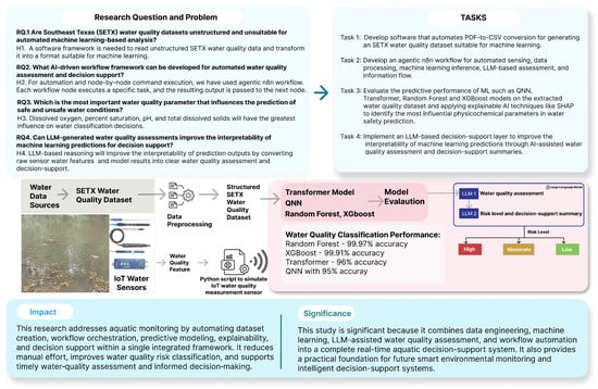
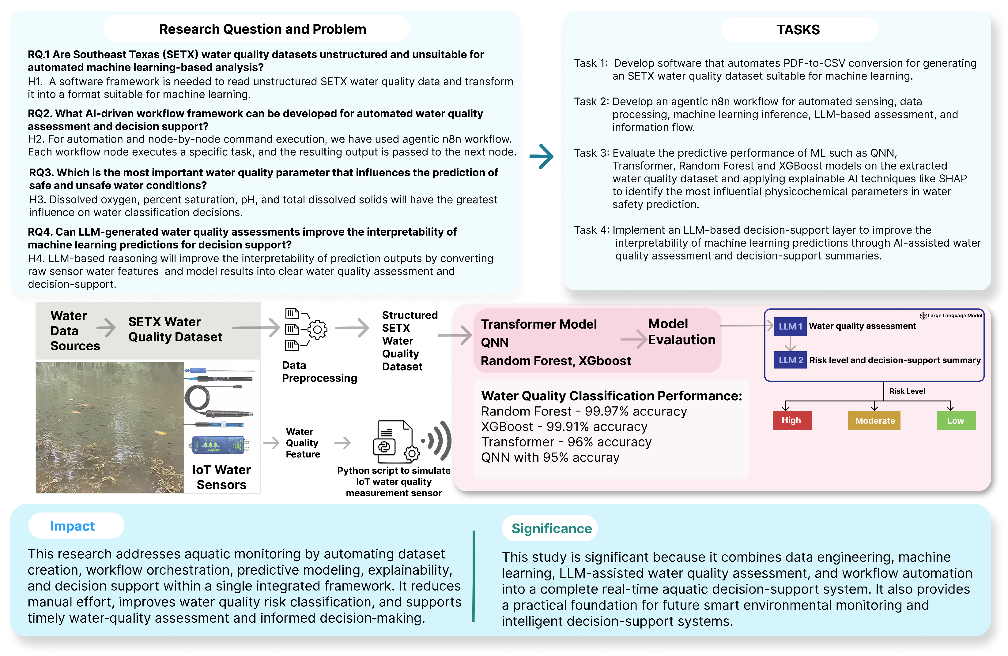
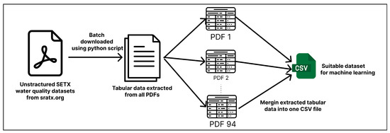
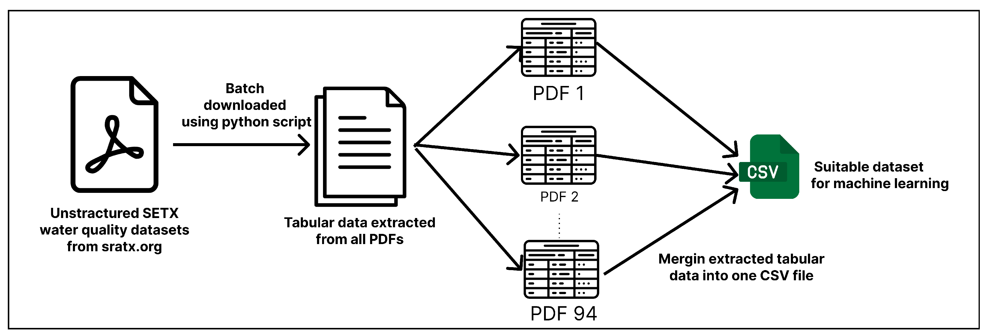
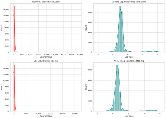
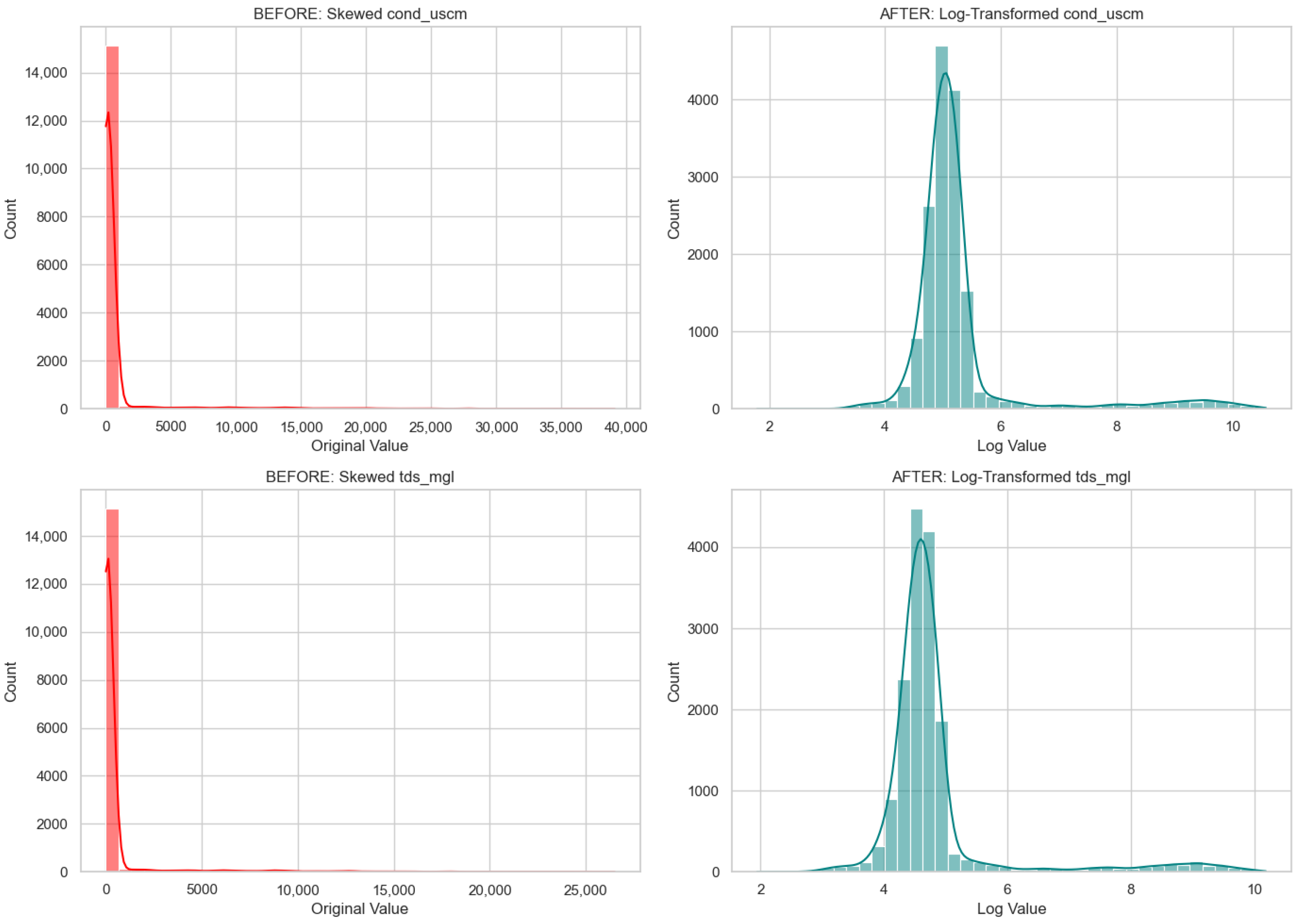
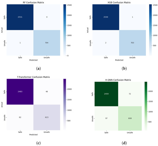
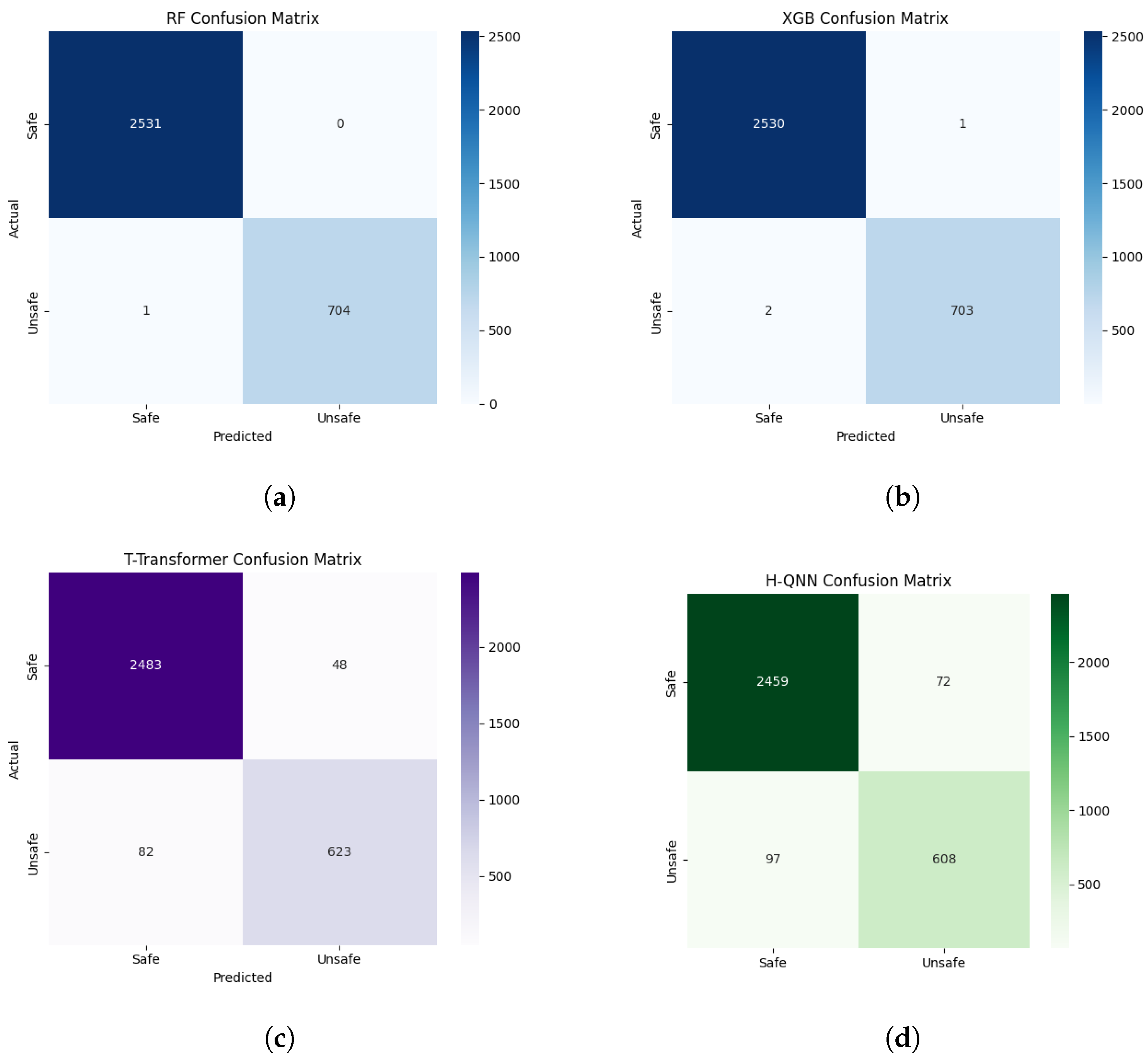
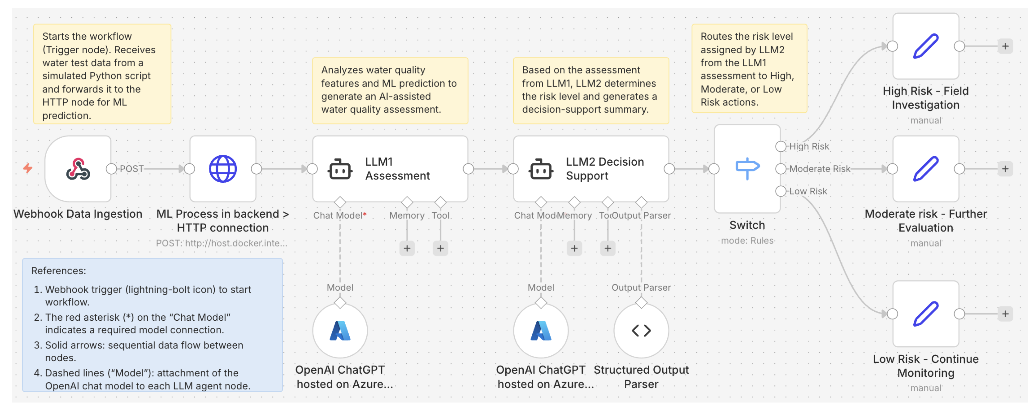
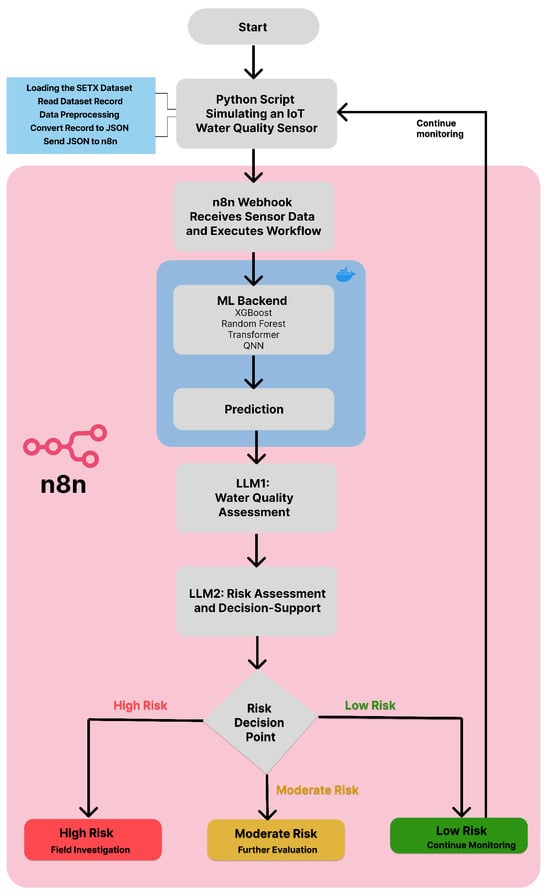
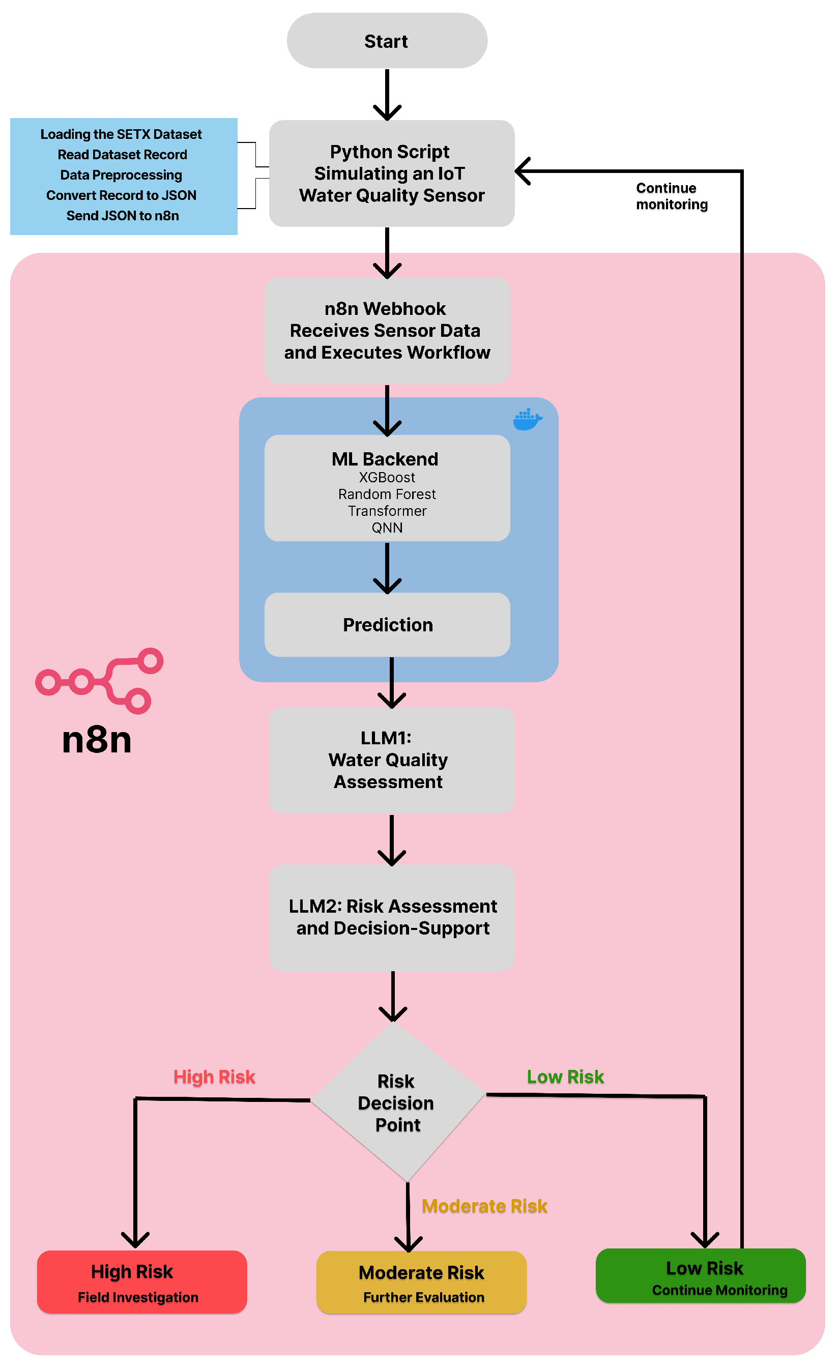
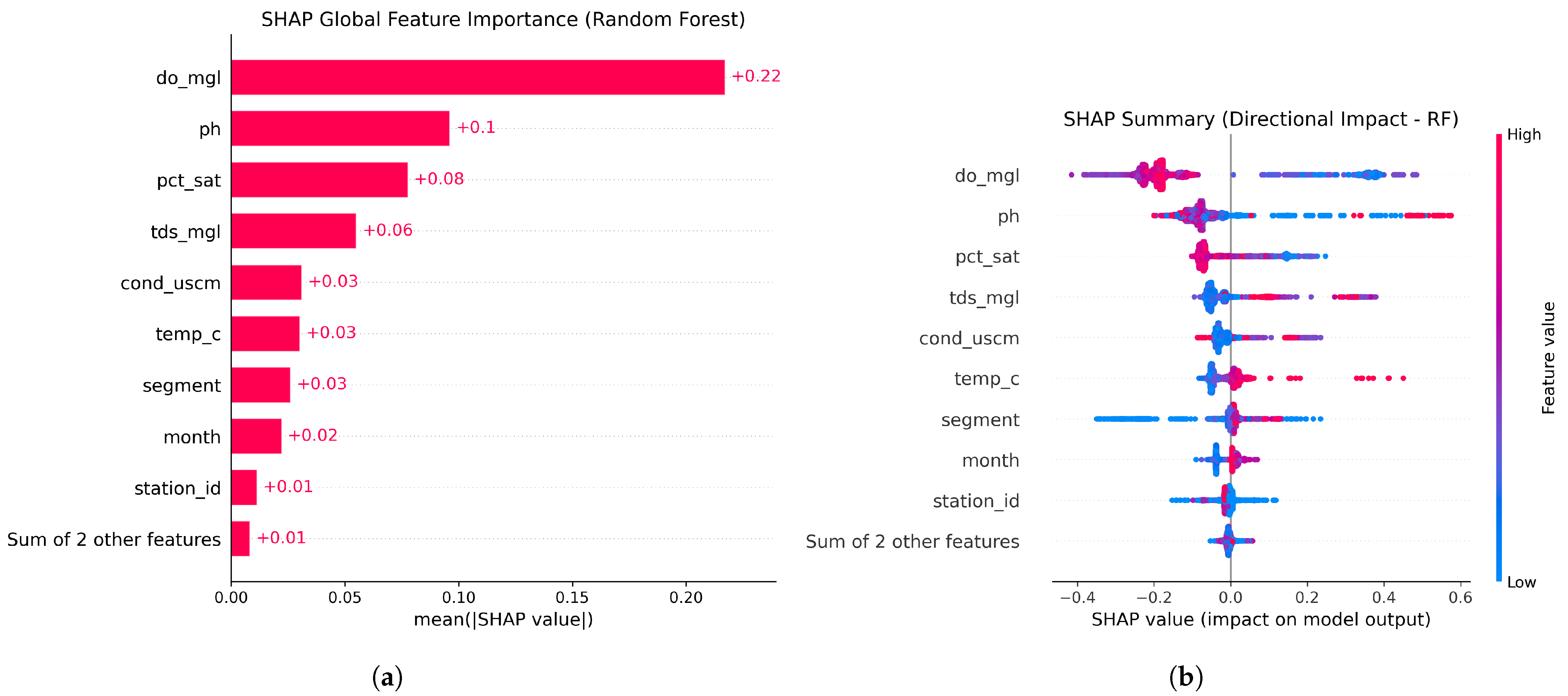
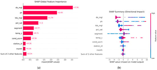
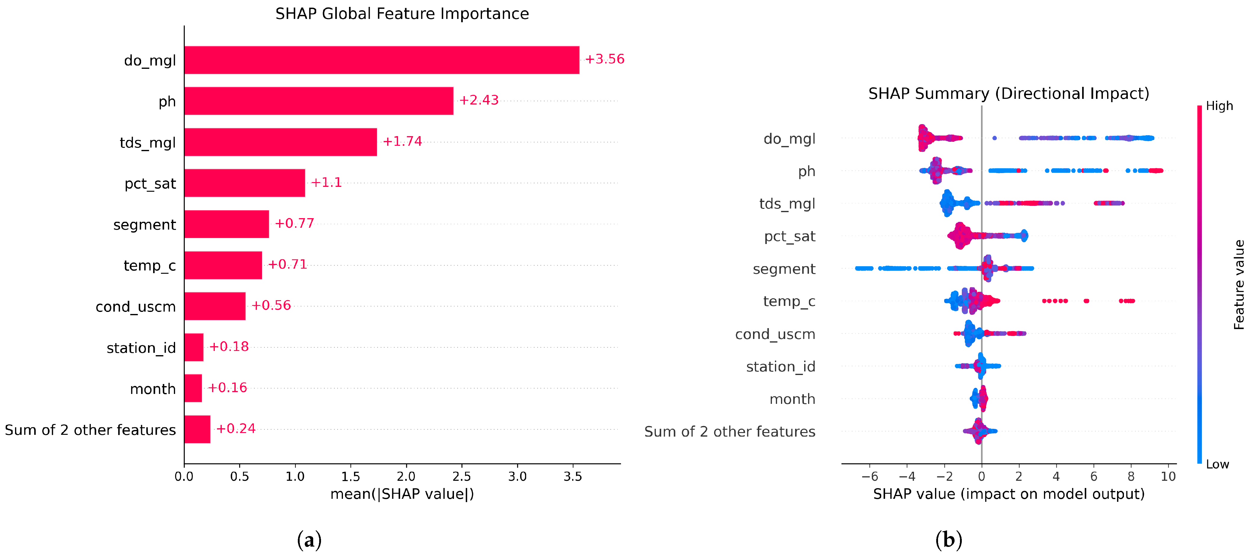
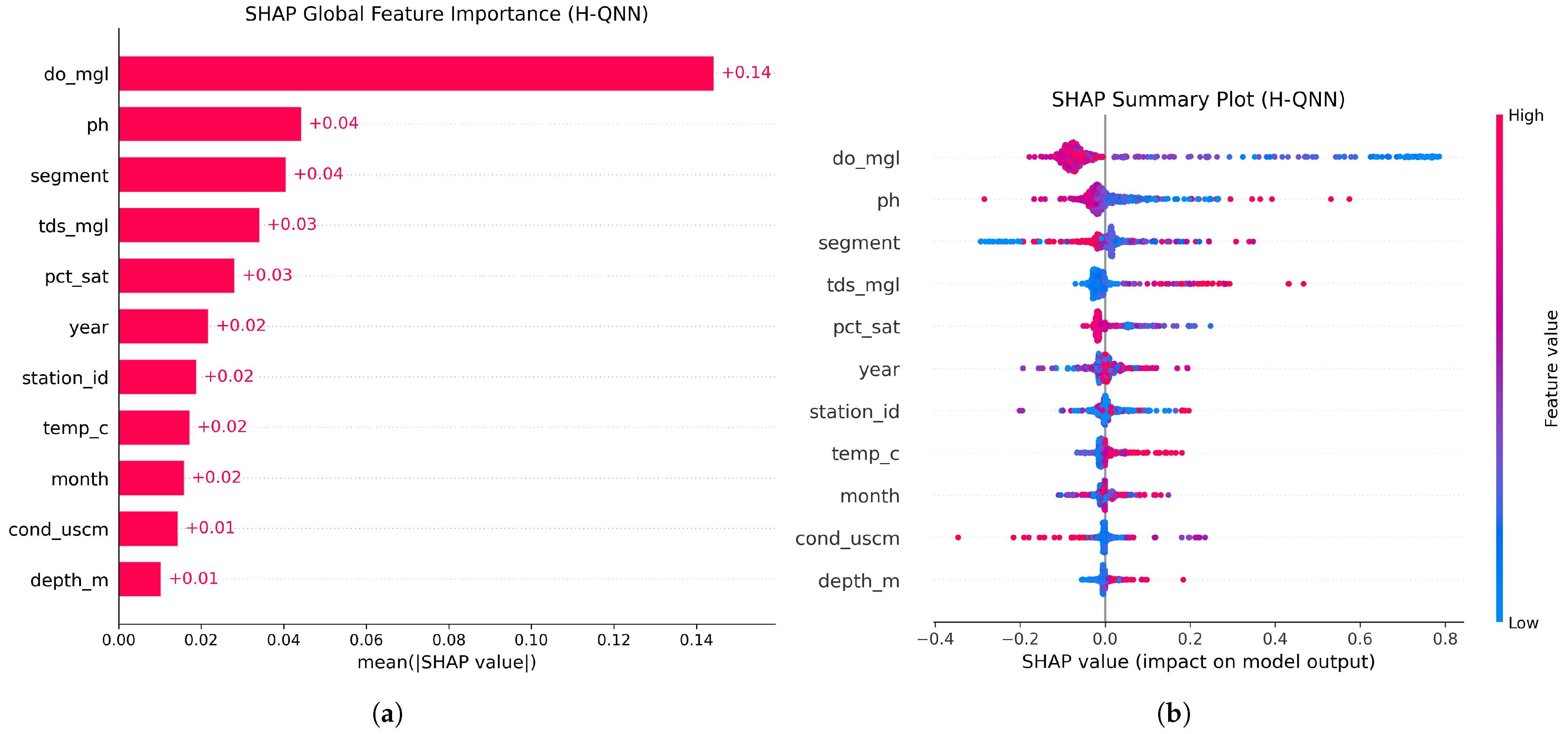
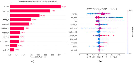
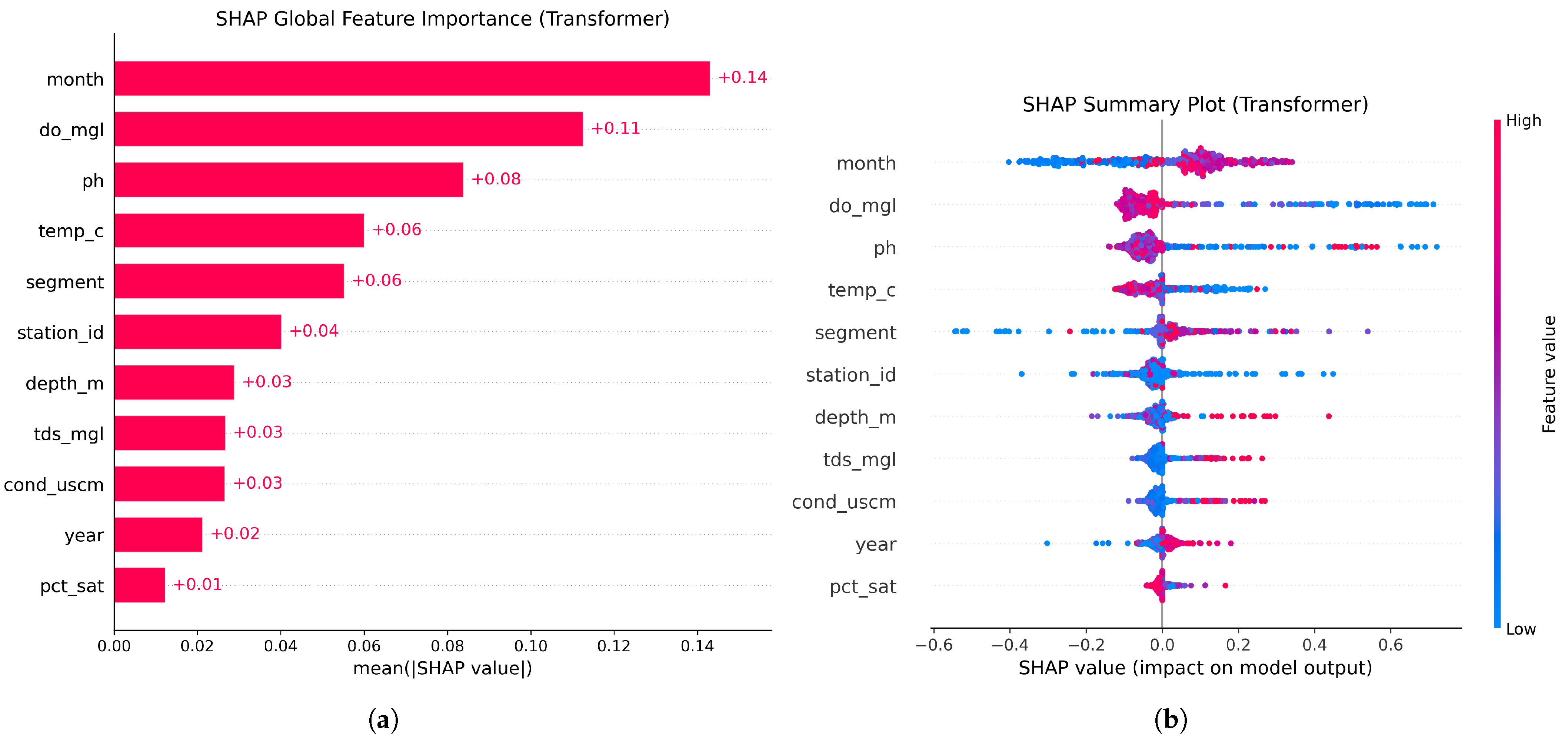
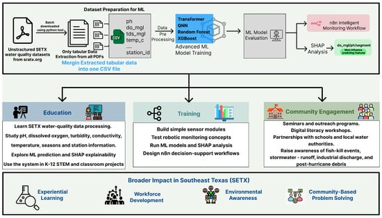
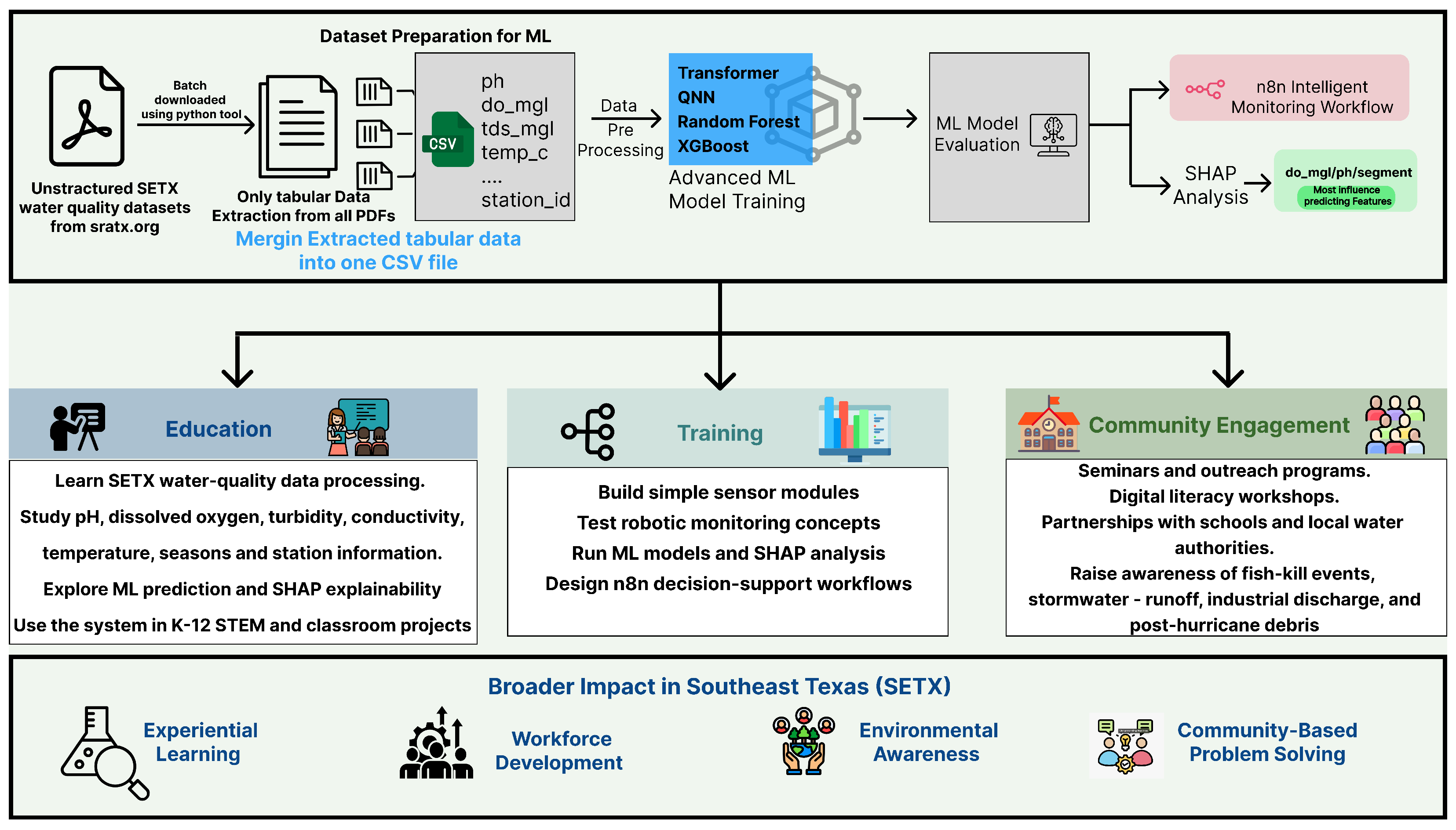

Disclaimer/Publisher’s Note: The statements, opinions and data contained in all publications are solely those of the individual author(s) and contributor(s) and not of MDPI and/or the editor(s). MDPI and/or the editor(s) disclaim responsibility for any injury to people or property resulting from any ideas, methods, instructions or products referred to in the content. |
© 2026 by the authors. Licensee MDPI, Basel, Switzerland. This article is an open access article distributed under the terms and conditions of the Creative Commons Attribution (CC BY) license.