Strong Convergence of a Unified Family of Shrinking Double Inertial Iterative Frameworks with Application to Air Quality Prediction

Abstract

In this paper, we propose a shrinking double inertial framework for approximating common fixed points of a countable family of quasi-nonexpansive mappings in Hilbert spaces. The framework combines a shrinking projection technique with a double inertial extrapolation mechanism, and strong convergence of the generated sequence is established under suitable assumptions. The shrinking strategy ensures strong convergence to a common fixed point, whereas the double inertial terms introduce additional extrapolation flexibility into the iterative process. To illustrate the theoretical results, a numerical example in an infinite-dimensional function space is presented using quasi-nonexpansive mappings. Motivated by variational inequality problems involving monotone and Lipschitz continuous operators, two further shrinking double inertial algorithms are developed using projected gradient and extragradient-type constructions. The proposed algorithms are then incorporated into Extreme Learning Machine models for air quality prediction. Experiments are conducted for five target pollutants, namely, NOx(GT), NMHC(GT), C₆H₆(GT), CO(GT), and NO₂(GT), using target-specific MRMR-selected feature sets. Predictive performance is evaluated using RMSE, MAE, and $R^2$. The numerical results show that the proposed algorithms achieve competitive predictive performance across the five targets. The projected gradient and extragradient frameworks exhibit complementary behavior depending on the target variable and problem structure, suggesting that different variational mapping constructions may be suitable for different prediction tasks. These findings demonstrate the theoretical flexibility and practical applicability of the proposed frameworks to fixed-point problems, variational inequalities, and constrained machine learning models.

1. Introduction

Throughout this paper, let $\mathcal{H}$ be a real Hilbert space endowed with the inner product $⟨·,·⟩$ and induced norm $\parallel ·\parallel$, and let C be a nonempty, closed, and convex subset of $\mathcal{H}$. A mapping $T:C\to C$ is called nonexpansive if

$$\parallel Tx-Ty\parallel \le \parallel x-y\parallel \mathrm{for}\mathrm{all}x,y\in C$$

and quasi-nonexpansive if the fixed-point set $F\left(T\right):=\{x\in C:Tx=x\}$ is nonempty and

$$\parallel Tx-p\parallel \le \parallel x-p\parallel \mathrm{for}\mathrm{all}x\in C\mathrm{and}p\in F\left(T\right).$$

The problem of finding a fixed point of such mappings—and, more generally, a common fixed point of a finite or countable family $\left\{T_i\right\}$—arises naturally in convex feasibility problems, variational inequalities, equilibrium problems, monotone inclusions, image reconstruction, and signal recovery [1,2].

The most elementary scheme for fixed-point approximation is the Mann iteration [3]:

$$x_{k+1}=(1-{\alpha }_k)x_k+{\alpha }_{k}T{x}_k,{\alpha }_k\in [0,1].$$

(1)

To enlarge the class of admissible iterations, Ref. [4] introduced the celebrated two-step iteration:

$$\left\{\begin{array}{cc}\hfill y_k& =(1-{\beta }_k)x_k+{\beta }_{k}T{x}_k,\hfill \\ \hfill x_{k+1}& =(1-{\alpha }_k)x_k+{\alpha }_{k}T{y}_k,\hfill \end{array}\right.$$

(2)

with ${\alpha }_k,{\beta }_k\in [0,1]$. The Ishikawa iteration reduces to Mann’s scheme when ${\beta }_k=0$, and the additional intermediate step $y_k$ has proven crucial for establishing convergence over broader classes of mappings, including strict pseudocontractions [5] and asymptotically nonexpansive mappings [6]. Subsequent multi-step generalizations include Noor’s three-step iteration [7], the S-iteration of [8], and the SP-iteration [9].

A well-known obstacle for both (1) and (2) is that they generally produce only weak convergence in infinite-dimensional Hilbert spaces [10], which is insufficient for many applications where strong convergence is essential. Several remedies have been proposed: the Halpern iteration [11], the CQ (hybrid) method of [12], and the shrinking projection method of [13]. The latter scheme, designed for a family $\left\{T_k\right\}$ of nonexpansive mappings, is defined by

$$\left\{\begin{array}{cc}\hfill y_k& ={\alpha }_k{x}_k+(1-{\alpha }_k)T_k{x}_k,\hfill \\ \hfill C_{k+1}& =\{z\in C_k:\parallel y_k-z\parallel \le \parallel x_k-z\parallel \},\hfill \\ \hfill x_{k+1}& =P_{C_{k+1}}{x}_0,\hfill \end{array}\right.$$

(3)

where $C_1=C$ and $P_C$ denotes the metric projection onto a closed convex set C. Under the NST-condition between $\left\{T_k\right\}$ and a target mapping T [14], the sequence $\left\{x_k\right\}$ converges strongly to $P_{F\left(T\right)}{x}_0$. The shrinking projection method has since become a cornerstone of strong-convergence theory and has been extended to firmly nonexpansive mappings [14], quasi-nonexpansive mappings, and Banach-space settings.

The natural next step is to integrate the Ishikawa-type two-step structure with the shrinking framework, particularly to approximate a common fixed point of two mappings simultaneously. This was carried out recently by [15], who proposed a unified scheme combining the Ishikawa iteration, the hybrid (shrinking) projection, and the mean-valued iteration. For two quasi-nonexpansive mean-demiclosed mappings S and T, the essential form reads

$$\left\{\begin{array}{cc}\hfill w_k& ={\lambda }_k{x}_k+(1-{\lambda }_k)S{x}_k,\hfill \\ \hfill z_k& ={\nu }_k{w}_k+(1-{\nu }_k)T{w}_k,\hfill \\ \hfill C_{k+1}& =\{h\in C_k:\parallel z_k-h\parallel \le \parallel x_k-h\parallel \},\hfill \\ \hfill x_{k+1}& =P_{C_{k+1}}{x}_0,\hfill \end{array}\right.$$

(4)

with ${\lambda }_k,{\nu }_k\in [0,1]$. Iteration (4) converges strongly to $P_{F\left(S\right)\cap F\left(T\right)}{x}_0$ without continuity or commutativity assumptions on S and T, unifying the strong-convergence advantage of shrinking projection with the flexibility of two-step iteration over two distinct mappings.

Parallel to the developments above, inertial extrapolation has emerged as a powerful technique for accelerating iterative methods. Originating with Polyak’s heavy-ball method for smooth optimization [16],

$$x_{k+1}=x_k-{\lambda }_k\nabla f\left(x_k\right)+{\theta }_k(x_k-x_{k-1}),$$

(5)

the inertial term ${\theta }_k(x_k-x_{k-1})$ was adapted to monotone inclusions by [17] through the inertial proximal point algorithm. For fixed-point iterations, Mainge [18] introduced the inertial Mann iteration:

$$\left\{\begin{array}{cc}\hfill y_k& =x_k+{\theta }_k(x_k-x_{k-1}),\hfill \\ \hfill x_{k+1}& =(1-{\alpha }_k)y_k+{\alpha }_{k}T{y}_k.\hfill \end{array}\right.$$

(6)

Inertial extrapolation has since been incorporated into virtually every major iterative framework, including the Krasnosel’skiĭ–Mann iteration [19], forward–backward splitting [20], and the shrinking projection method [21], consistently yielding faster convergence in both theory and numerical practice.

More recently, double inertial (or two-step inertial) extrapolation has emerged as a further refinement, in which two consecutive momentum terms are used:

$${\nabla }_k={\theta }_k(x_k-x_{k-1})+{\delta }_k(x_{k-1}-x_{k-2}),y_k=x_k+{\nabla }_k.$$

(7)

This construction, analogous in spirit to higher-order multistep methods in numerical analysis, exploits the deeper memory of the iterate trajectory and has been shown to outperform single-inertial variants on various test problems [22].

Despite the substantial progress along each of the four directions outlined above—two-step iteration, shrinking projection, two-mapping common-fixed-point schemes, and inertial acceleration—to the best of our knowledge, no existing algorithm simultaneously combines all of these features. In particular, the integration of double inertial extrapolation into a shrinking two-step Mann scheme for families $\left\{T_{1,k}\right\}$ and $\left\{T_{2,k}\right\}$ of nonexpansive (or quasi-nonexpansive) mappings satisfying the NST_w-condition has not been investigated. Such a combination is both natural and desirable: shrinking projection delivers strong convergence; the two-step structure enables flexible handling of two (or more) mappings; and double inertial extrapolation provides acceleration beyond what single-inertial schemes can achieve.

Motivated by these observations, our main contributions are summarized as follows:

• We establish a strong convergence theorem (Theorem 1) for the SDITMA iteration to the common fixed point of a countable family of quasi-nonexpansive mappings.
• We provide explicit and mild conditions on the inertial parameters $\left\{{\theta }_k\right\},\left\{{\delta }_k\right\}$ and on the relaxation parameters $\left\{{\alpha }_k\right\},\left\{{\beta }_k\right\}$ ensuring convergence.
• We compare the proposed scheme numerically against representative algorithms in the literature, including (4), demonstrating the practical advantages of double inertial extrapolation in the shrinking two-step setting.
• We further develop variational inequality-based extensions of the proposed framework and apply them to Extreme Learning Machine models for air quality prediction. Numerical results on five benchmark pollutants demonstrate that different variational mapping strategies exhibit complementary predictive strengths, highlighting the flexibility of the proposed framework for both optimization and data-driven learning applications.

2. Preliminaries

Let $\mathcal{H}$ be a real Hilbert space endowed with an inner product $⟨.,.⟩$ and the induced norm $\parallel .\parallel$.

Definition 1.

A mapping $A:\mathcal{H}\to \mathcal{H}$ is said to be

1. $monotone$ if, for each $a,b\in \mathcal{H}$,

$$⟨Aa-Ab,a-b⟩\ge 0;$$

2. $maximal$ monotone if it is monotone and its graph

$$G\left(A\right):=\left\{\right(a,Aa):a\in \mathcal{H}\}$$

is not a proper subset of one of any other monotone mapping;

3. L-$Lipschitzcontinuous$ if there is a constant $L>0$ such that

$$\parallel Aa-Ab\parallel \le L\parallel a-b\parallel \mathit{for}\mathit{all}a,b\in \mathcal{H};$$

4. $firmlynonexpansive$ if

$${\parallel Aa-Ab\parallel }^2\le {\parallel a-b\parallel }^2-{\parallel (I-A)a-(I-A)b\parallel }^2\mathit{for}\mathit{all}a,b\in \mathcal{H},$$

or equivalently,

$$⟨Aa-Ab,a-b⟩\ge {\parallel Aa-Ab\parallel }^2\mathit{for}\mathit{all}a,b\in \mathcal{H};$$

5. α-cocoercive or α-$inversestronglymonotone$ if $\alpha A$ is firmly nonexpansive when $\alpha >0$.

Let $\mathcal{C}$ be a nonempty closed convex subset of $\mathcal{H}$ and $A:\mathcal{H}\to \mathcal{H}$. The variational inequality problem (VIP) can be formulated as the problem of finding a point $a^{*}\in \mathcal{C}$ such that

$$⟨A{a}^{*},a-a^{*}⟩\ge 0,\forall a\in \mathcal{C}.$$

(8)

The set of solutions of VIP (8) is denoted by $VI(\mathcal{C},A)$. The classical variational inequality was first introduced by Hartman and Stampacchia [23] in 1966 in Euclidean spaces.

Let $\mathcal{H}$ be a Hilbert space and let C be a subset of $\mathcal{H}$. Let $\left\{T_k\right\}$ and $\tau$ be two families of mappings of C into itself such that F($\tau$), ${\cap }_{k=1}^{\infty }F\left(T_k\right)$ are nonempty sets, where $F\left(T_k\right)$ is the set of all fixed points of $T_k$ and $F\left(\tau \right)$ is the set of all common fixed points of $\tau$. $\left\{T_k\right\}$ is said to satisfy the $NS{T}_w$-condition with respect to $\tau$ if, for each bounded sequence $\left\{a_k\right\}$ in C, there exists a subsequence $\left\{a_{k_j}\right\}$ of $\left\{a_k\right\}$ such that

$$\begin{array}{c}\hfill \underset{k\to \infty }{\lim }\parallel a_k-T_k{a}_k\parallel =0.\Rightarrow \underset{k\to \infty }{\lim }\parallel a_{k_j}-T{a}_{k_j}\parallel =0,\forall T\in \tau .\end{array}$$

It is obvious that if $\left\{T_k\right\}$ satisfies the $NST$-condition with respect to $\tau$, then $\left\{T_k\right\}$ satisfies the $NS{T}_w$-condition with respect to $\tau$. The state of $NS{T}_w$-condition was proposed in [24]. The following lemma is taken from Cholamjiak [24].

Lemma 1

([24]). Let $\mathcal{C}$ be a nonempty closed convex subset of a real Hilbert $\mathcal{H}$ and let $A:\mathcal{H}\to \mathcal{H}$ be a monotone and L-Lipschitz continuous mapping. For $\lambda >0$, define $T:=P_{\mathcal{C}}(I-\lambda A)$. Then, $I-T$ is demiclosed at 0.

Lemma 2

([24]). Let $\mathcal{C}$ be a nonempty closed convex subset of a real Hilbert $\mathcal{H}$ and let $A:\mathcal{H}\to \mathcal{H}$ be a monotone and L-Lipschitz continuous mapping. For $\lambda \in (0,{\displaystyle \frac{1}{L}}]$, define $T:=P_{\mathcal{C}}(I-\lambda A{P}_{\mathcal{C}}(I-\lambda A))$. Then, $I-T$ is demiclosed at 0.

Lemma 3

([24]). Let $\mathcal{C}$ be a nonempty closed convex subset of $\mathcal{H}$ and let $A:\mathcal{H}\to \mathcal{H}$ be a monotone and L-Lipschitz continuous mapping. Let $\left\{{\lambda }^k\right\}$ be a bounded sequence in $(0,\infty )$ such that ${\displaystyle \underset{k\to \infty }{\lim \inf }{\lambda }^k>0}$ and $\lambda \in {\omega }_w\left({\lambda }^k\right)$, where ${\omega }_w\left({\lambda }^k\right)$ is the set of all cluster point of ${\lambda }^k$. Then, the family of mappings $\left\{T^k\right\}$ satisfies the $NS{T}_w$-condition, where $T^k:=P_{\mathcal{C}}(I-{\lambda }^{k}A)$ with $\tau =\{T:=P_{\mathcal{C}}(I-\lambda A):\lambda \in {\omega }_w\left({\lambda }^k\right)\}$.

Lemma 4

([24]). Let $\mathcal{C}$ be a nonempty closed convex subset of $\mathcal{H}$ and let $A:\mathcal{H}\to \mathcal{H}$ be a monotone and L-Lipschitz continuous mapping. Let $\left\{{\lambda }^k\right\}$ be a sequence in $(0,\infty )$ such that $0<c\le {\lambda }^k\le d<{\displaystyle \frac{1}{L}}$ and $\lambda \in {\omega }_w\left({\lambda }^k\right)$, where ${\omega }_w\left({\lambda }^k\right)$ is the set of all cluster points of ${\lambda }^k$. Then, the family of mappings $\left\{T^k\right\}$ satisfies the $NS{T}_w$-condition, where $T^k:=P_{\mathcal{C}}(I-{\lambda }^{k}A{P}_{\mathcal{C}}(I-{\lambda }^{k}A))$ with $\tau =\{T:=P_C(I-\lambda A{P}_{\mathcal{C}}(I-\lambda A):\lambda \in {\omega }_w\left({\lambda }^k\right)\}$.

We note that if $\lambda \in (0,{\displaystyle \frac{1}{L}}]$ and $0<c\le {\lambda }^k\le d<{\displaystyle \frac{1}{L}}$, then the mappings $P_{\mathcal{C}}(I-\lambda A)$, $P_{\mathcal{C}}\left(I-\lambda A{P}_{\mathcal{C}}(I-\lambda A)\right)$, $P_{\mathcal{C}}(I-{\lambda }^{k}A)$, $P_{\mathcal{C}}\left(I-{\lambda }^{k}A{P}_{\mathcal{C}}(I-{\lambda }^{k}A)\right)$ are quasi-nonexpansive; see [24].

Lemma 5

(Opial [25]). Let $\mathcal{H}$ be a Hilbert space and let $\left\{x_k\right\}$ be a sequence in $\mathcal{H}$. Suppose that there exists a nonempty subset $\Gamma \subset \mathcal{H}$ satisfying the following conditions:

$\left(i\right)$ for every $p\in \Gamma$ the limit $\underset{k\to +\infty }{\lim }\parallel x_k-p\parallel$ exists;

$\left(ii\right)$ Every weak-cluster point of the sequence $\left\{x_k\right\}$ belongs to Γ.

Then, there exists $x^{*}\in \Gamma$ such that the sequence $\left\{x_k\right\}$ weakly converges to $x^{*}$.

Lemma 6

([26]). Let $T:\mathcal{C}\to \mathcal{C}$ be a nonexpansive mapping on a closed and convex subset $\mathcal{C}$ of a Hilbert space $\mathcal{H}$. If T has a fixed point, then $I-T$ is demiclosed, that is, whenever a sequence $\left\{u_k\right\}$ in $\mathcal{C}$ weakly converges to $u\in \mathcal{C}$ and the sequence $\{u_k-T{u}_k\}$ strongly converges to y, it follows that $u-Tu=y$.

Lemma 7

([24]). Let C be a nonempty closed convex subset of $\mathcal{H}$ and let $A:\mathcal{H}\to \mathcal{H}$ be an α-inverse-strongly monotone. Then,

$\left(i\right)$ A is ${\displaystyle \frac{1}{\alpha }}$-Lipschitz continuous and monotone;

$\left(ii\right)$ if $\lambda \in (0,2\alpha ]$, then $(I-\lambda A)$ is nonexpansive.

Lemma 8

([17]). Let $\left\{{\gamma }_k\right\},\left\{{\delta }_k\right\},$ and $\left\{{\alpha }_k\right\}$ be the sequences in $[0,+\infty )$ such that

$$\begin{array}{c}\hfill {\gamma }_{k+1}\le {\gamma }_k+{\alpha }_k({\gamma }_k-{\gamma }_{k-1})+{\delta }_k\mathit{for}\mathit{all}k\ge 1,\end{array}$$

${\sum }_{k=1}^{\infty }{\delta }_k<+\infty$, and there exists a real number α with $0\le {\alpha }_k\le \alpha <1$ for all $k\ge 1$. Then, the following are

$\mathit{valid}:{\sum }_{k\ge 1}{[{\gamma }_k-{\gamma }_{k-1}]}_{+}<+\infty$, where ${\left[t\right]}_{+}=\max \{t,0\}$;

$\left(ii\right)$ There exists ${\gamma }^{*}\in [0,+\infty )$ such that ${\lim }_{k\to +\infty }{\gamma }_k={\gamma }^{*}$.

Lemma 9

([27]). Let $C\subset \mathcal{H}$ be a nonempty, closed, and convex subset of a real Hilbert space $\mathcal{H}$. For any $x,y,z\in \mathcal{H}$ and $a\in \mathbb{R}$, the set

$$\left\{{v\in C:\parallel y-v\parallel }^2\le {\parallel x-v\parallel }^2+⟨z,v⟩+a\right\}$$

is convex and closed.

Lemma 10

([12]). Let $C\subset \mathcal{H}$ be a nonempty, closed, and convex subset of a real Hilbert space $\mathcal{H}$, and let $P_C:\mathcal{H}\to C$ denote the metric projection from $\mathcal{H}$ onto C. Then, for all $x\in \mathcal{H}$ and $y\in C$, the following inequality holds:

$$\parallel y-P_C{x\parallel }^2+\parallel x-P_C{x\parallel }^2\le {\parallel x-y\parallel }^2.$$

3. Convergence Analysis

The proposed algorithm is developed by integrating a double inertial extrapolation strategy with the Ishikawa-type iterative framework and the shrinking projection method to achieve strong convergence in Hilbert spaces for two families of quasi-nonexpansive mappings. The incorporation of double inertial terms is intended to accelerate the iterative process by utilizing information from previous iterations, while the Ishikawa structure enhances the flexibility of the iterative scheme. Furthermore, the shrinking projection mechanism guarantees feasibility and establishes strong convergence of the generated sequence toward the desired solution set. Let $\mathcal{H}$ be a real Hilbert space and let $\mathcal{C}$ be a nonempty closed convex subset of $\mathcal{H}$. Assume that ${\left\{T_{i,k}\right\}}_{i=1}^2$ and $\tau$ are families of quasi-nonexpansive mappings from H into itself. The complete computational procedure of the proposed method is presented in Algorithm 1.

Algorithm 1 Shrinking Double Inertial Two-steps Mann Algorithm (SDITMA)

Initialization: Let $x_{-1},x_0,x_1\in \mathcal{H}$ be arbitrary, ${\theta }_k,{\delta }_k\in (-\infty ,\infty ),{\alpha }_k,{\beta }_k\in (0,1)$ for all $k\ge 1$. Set ${\mathcal{C}}_1=\mathcal{C}$, Step 1. For $k=1$, compute $$y_k=x_k+{\nabla }_k,$$ where ${\nabla }_k={\theta }_k(x_k-x_{k-1})+{\delta }_k(x_{k-1}-x_{k-2}).$ Step 2. Compute $$z_k=(1-{\alpha }_k)y_k+{\alpha }_k{T}_{1,k}{y}_k.$$ Step 3. Compute $$t_k=(1-{\beta }_k)z_k+{\beta }_k{T}_{2,k}{z}_k.$$ Step 4. Compute $${\mathcal{C}}_{k+1}=\{u\in {\mathcal{C}}_k:\parallel t_k{-u\parallel }^2\le \parallel x_k{-u\parallel }^2+2⟨{\nabla }_k,x_k-u⟩+\parallel {\nabla }_k{\parallel }^2\}.$$ Step 5. Compute $$x_{k+1}=P_{{\mathcal{C}}_{k+1}}{x}_0.$$ Then, update $k:=k+1$ and return to Step 1.

Theorem 1.

Let $\mathcal{H}$ be a real Hilbert space. Let ${\left\{T_{i,k}\right\}}_{i=1}^2$ and τ be family of quasi-nonexpansive such that $\left\{T_{i,k}\right\}$ satisfies the $NS{T}_w$-condition with respect to τ for all $i=1,2$. Suppose that F(τ), ${\cap }_{k=1}^{\infty }{\cap }_{i=1}^2$ F($T_{i,k}$) are nonempty sets. Let $\left\{x_k\right\}$ be defined by Algorithm 1. Assume that the following conditions are satisfied:

(i)

${\lim }_{k\to \infty }$$|{\theta }_k|$$\parallel x_k-x_{k-1}\parallel =0$;

(ii)

${\lim }_{k\to \infty }$$|{\delta }_k|$$\parallel x_{k-1}-x_{k-2}\parallel =0$;

(iii)

$0<{\text{lim inf}}_{k\to \infty }{\alpha }_k\le {\text{lim sup}}_{k\to \infty }{\alpha }_k<1$ and $0<{\text{lim inf}}_{k\to \infty }{\beta }_k\le {\text{lim sup}}_{k\to \infty }{\beta }_k<1$;

(iv)

$I-T$ is demiclosed at 0 for all $T\in \tau$.

Then, $\left\{x_k\right\}$ converges strong to a point in F(τ).

Proof. 

We split the proof into five steps.

• Step 1. Show that $P_{{\mathcal{C}}_{k+1}}{x}_0$ is well-defined for each $x_0\in \mathcal{H}$.

From the definition of ${\mathcal{C}}_{k+1}$, from Lemma 9, ${\mathcal{C}}_{k+1}$ is closed and convex for each $k\ge 1$. For each $k\in \mathbb{N}$, let $q\in {\cap }_{k=1}^{\infty }{\cap }_{i=1}^{2}F\left(T_{i,k}\right)$. Since $T_1,k$ and $T_2,k$ are quasi-nonexpansive, this implies that

$$\begin{array}{cc}\hfill \parallel t_k{-q\parallel }^2& \le (1-{\beta }_k)\parallel z_k{-q\parallel }^2+{\beta }_k\parallel T_{2,k}{z}_k{-q\parallel }^2-(1-{\beta }_k){\beta }_k{\parallel z_k-T_{2,k}{z}_k\parallel }^2\hfill \\ \hfill & \le \parallel z_k{-q\parallel }^2-(1-{\beta }_k){\beta }_k{\parallel z_k-T_{2,k}{z}_k\parallel }^2\hfill \\ \hfill & =(1-{\alpha }_k)\parallel y_k{-q\parallel }^2+{\alpha }_k\parallel T_{1,k}{y}_k{-q\parallel }^2-(1-{\alpha }_k){\alpha }_k{\parallel y_k-T_{1,k}{y}_k\parallel }^2\hfill \\ \hfill & -(1-{\beta }_k){\beta }_k{\parallel z_k-T_{2,k}{z}_k\parallel }^2\hfill \\ \hfill & \le \parallel y_k{-q\parallel }^2-(1-{\alpha }_k){\alpha }_k\parallel y_k-T_{1,k}{y}_k{\parallel }^2-(1-{\beta }_k){\beta }_k{\parallel z_k-T_{2,k}{z}_k\parallel }^2\hfill \\ \hfill & =\parallel x_k+{\nabla }_k{-q\parallel }^2-(1-{\alpha }_k){\alpha }_k\parallel y_k-T_{1,k}{y}_k{\parallel }^2-(1-{\beta }_k){\beta }_k{\parallel z_k-T_{2,k}{z}_k\parallel }^2\hfill \\ \hfill & =\parallel x_k{-q\parallel }^2+2⟨{\nabla }_k,x_k-q⟩+\parallel {\nabla }_k{\parallel }^2-(1-{\alpha }_k){\alpha }_k{\parallel y_k-T_{1,k}{y}_k\parallel }^2\hfill \\ \hfill & -(1-{\beta }_k){\beta }_k{\parallel z_k-T_{2,k}{z}_k\parallel }^2\hfill \\ \hfill & \le \parallel x_k{-q\parallel }^2+2⟨{\nabla }_k,x_k-q⟩+{\parallel {\nabla }_k\parallel }^2.\hfill \end{array}$$

(9)

Therefore, we have $q\in {\mathcal{C}}_{k+1}$; thus, ${\cap }_{k=1}^{\infty }{\cap }_{i=1}^{2}F\left(T_{i,k}\right)\subset {\mathcal{C}}_{n+1}$. Therefore, $P_{{\mathcal{C}}_{k+1}}{x}_0$ is well defined.

• Step 2: Prove that ${\displaystyle \underset{n\to \infty }{\lim }\parallel x_n-x_0\parallel }$ exists. Since ${\cap }_{k=1}^{\infty }{\cap }_{i=1}^{2}F\left(T_{i,k}\right)$ is a nonempty, closed, and convex subset of $\mathcal{H}$, there exists a unique point $p^{*}\in {\cap }_{k=1}^{\infty }{\cap }_{i=1}^{2}F\left(T_{i,k}\right)$ such that $p*=P_{{\cap }_{k=1}^{\infty }{\cap }_{i=1}^{2}F\left(T_{i,k}\right)}{x}_0$. From the fact that $x_k=P_{{\mathcal{C}}_k}{x}_0$ and $x_{k+1}\in {\mathcal{C}}_{k+1}\subset {\mathcal{C}}_k$ for all $k\in \mathbb{N}$, it follows that

  $$\parallel x_k-x_0\parallel \le \parallel x_{k+1}-x_0\parallel ,\forall k\ge 0.$$

  On the other hand, since ${\cap }_{k=1}^{\infty }{\cap }_{i=1}^{2}F\left(T_{i,k}\right)\subset {\mathcal{C}}_k$ for all $k\ge 0$, we obtain

  $$\parallel x_k-x_0\parallel \le \parallel p^{*}-x_0\parallel ,\forall k\ge 0.$$

  Hence, the sequence $\left\{x_k\right\}$ is nondecreasing and bounded. Therefore, ${\displaystyle \underset{k\to \infty }{\lim }\parallel x_k-x_0\parallel }$ exists.
• Step 3: Show that $x_k\to q^{*}\in \mathcal{C}$ as $k\to \infty$. For $m>k$, by the definition of ${\mathcal{C}}_k$, we see that $x_m=P_{{\mathcal{C}}_m}{x}_0\in {\mathcal{C}}_m\subset {\mathcal{C}}_n$. From Lemma 10, we have

  $$\parallel x_m-x_k{\parallel }^2\le \parallel x_m-x_0{\parallel }^2-{\parallel x_k-x_0\parallel }^2.$$

From Step 2, we obtain that $\left\{x_k\right\}$ is a Cauchy sequence. Hence, there exists $q^{*}\in \mathcal{H}$ such that $x_k\to q^{*}$ as $k\to \infty$. In particular, we have

$$\begin{array}{c}\hfill \underset{k\to \infty }{\lim }\parallel x_{k+1}-x_k\parallel =0.\end{array}$$

(10)

• Step 4: Show that $q^{*}\in F\left(\tau \right)$. From $x_{k+1}\in \mathcal{C}$, we have

  $$\begin{array}{c}\hfill \parallel t_k-x_{k+1}\parallel \le \sqrt{\parallel x_k-x_{k+1}{\parallel }^2+2⟨{\nabla }_k,x_k-x_{k+1}⟩+{\parallel {\nabla }_k\parallel }^2}.\end{array}$$

  (11)

  From (10) and conditions (i), (ii), we obtain

  $$\begin{array}{c}\hfill \parallel t_k-x_{k+1}\parallel \to 0.\end{array}$$

  This implies that

  $$\begin{array}{c}\hfill \parallel t_k-x_k\parallel \le \parallel t_k-x_{k+1}\parallel +\parallel x_{k+1}-x_k\parallel \to 0.\end{array}$$

  (12)

  From (9), we have

  $$\begin{array}{c}\hfill (1-{\alpha }_k){\alpha }_k\parallel y_k-T_{1,k}{y}_k{\parallel }^2+(1-{\beta }_k){\beta }_k\parallel z_k-T_{2,k}{z}_k{\parallel }^2\le \parallel x_k{-q\parallel }^2-{\parallel t_k-q\parallel }^2\\ \hfill +2⟨{\nabla }_k,x_k-u⟩+{\parallel {\nabla }_k\parallel }^2\\ \hfill \le \parallel x_k{-q\parallel }^2-{\parallel t_k-q\parallel }^2\\ \hfill +2\parallel {\nabla }_k\parallel \parallel x_k-u\parallel +\parallel {\nabla }_k{\parallel }^2\end{array}$$

  (13)

  and from the above Assumptions (i)-(iii) and (12) we have

  $$\underset{k\to \infty }{\lim }\parallel y_k-T_{1,k}{y}_k{\parallel }^2=\underset{k\to \infty }{\lim }{\parallel z_k-T_{2,k}{z}_k\parallel }^2=0.$$

  Combining this with the definition of $\left\{z_k\right\}$ and $\left\{t_k\right\}$, we have

  $$\begin{array}{c}\hfill \underset{k\to \infty }{\lim }\parallel t_k-z_k\parallel =\underset{k\to \infty }{\lim }{\beta }_k\parallel z_k-T_{2,k}{z}_k\parallel =0\end{array}$$

  (14)

  and

  $$\begin{array}{c}\hfill \underset{k\to \infty }{\lim }\parallel z_k-y_k\parallel =\underset{k\to \infty }{\lim }{\alpha }_k\parallel y_k-T_{1,k}{y}_k\parallel =0.\end{array}$$

  (15)

  From Step 3, (12), (14), and (15) we also have $y_k\to q^{*}$ and $z_k\to q^{*}$. Since $\left\{T_{1,k}\right\}$ and $\left\{T_{2,k}\right\}$ satisfy the $NS{T}_w$-condition with respect to $\tau$, there exists a subsequence $\left\{y_{k_j}\right\}$ of $\left\{y_k\right\}$ such that

  $$\begin{array}{c}\hfill \underset{j\to \infty }{\lim }\parallel y_{k_j}-\mathit{T}{y}_{k_j}\parallel =0,\mathrm{for}\mathrm{all}\mathit{T}\in \tau .\end{array}$$

  (16)

  By assumption (iv), $I-\mathit{T}$ is demiclosed at zero for all $\mathit{T}\in \tau$, and using (16) and again from Step 3, $q^{*}\in F\left(\tau \right)$. Therefore, $\left\{x_k\right\}$ converges strongly to $q^{*}\in F\left(\tau \right)$. This completes the proof.    □

We next present a numerical example in a function space to illustrate the applicability and convergence behavior of the proposed shrinking double inertial iterative frameworks. Let $\mathcal{H}=L^2\left([-1,0]\right)$ be the real Hilbert space of all square-integrable real-valued functions on $[-1,0]$. The inner product on $\mathcal{H}$ is defined by

$$⟨x,y⟩={\int }_{-1}^{0}x\left(t\right)y\left(t\right)dt,x,y\in L^2\left([-1,0]\right),$$

and the induced norm is given by

$$\parallel x\parallel ={\left({\int }_{-1}^0{\left|x\left(t\right)\right|}^{2}dt\right)}^{1/2}.$$

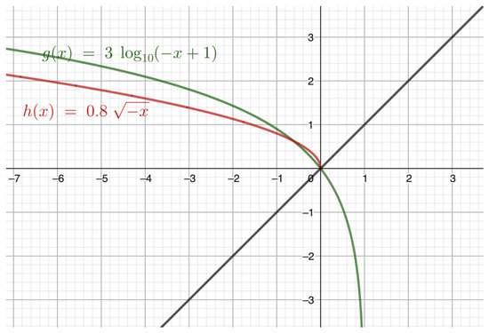
Let $\mathcal{C}$ be a nonempty closed convex subset of $L^2\left([-1,0]\right)$. In this numerical experiment, the mappings $T_{1,k}\left(x\left(t\right)\right)=3\log (-x\left(t\right)+1)$ and $T_{2,k}\left(x\left(t\right)\right)=0.8\sqrt{-x\left(t\right)}$ are defined on $\mathcal{C}$ and generated from the functions illustrated in Figure 1. Both mappings are quasi-nonexpansive but not nonexpansive, and they share the common fixed point

$$x\left(t\right)=0,t\in [-1,0],$$

that is,

$$F\left(T_1\right)\cap F\left(T_2\right)=\left\{0\right\}.$$

Figure 1. Illustration of the quasi-nonexpansive mappings $T_1$ and $T_2$ used in the numerical experiment. Both mappings share the common fixed point $x=0$, while neither mapping is nonexpansive.

To demonstrate the convergence behavior of the proposed Shrinking Double Inertial Two-step Mann Algorithm (SDITMA), we consider three different sets of initial functions in the Hilbert space $L^2\left([-1,0]\right)$. Throughout this experiment, the algorithmic parameters are fixed as ${\alpha }_k=0.5$, ${\beta }_k=0.5$,

$$\begin{array}{c}\hfill {\theta }_k=\left\{\begin{array}{c}{\displaystyle \frac{1}{k\parallel x_k-x_{k-1}\parallel }},\mathrm{if}k>N,\hfill \\ -10,\mathrm{otherwise},\hfill \end{array}\right.\end{array}$$

and

$$\begin{array}{c}\hfill {\delta }_k=\left\{\begin{array}{c}{\displaystyle \frac{1}{k\parallel x_{k-1}-x_{k-2}\parallel }},\mathrm{if}k>N,\hfill \\ -10,\mathrm{otherwise}.\hfill \end{array}\right.\end{array}$$

The following initial functions are employed:

Case 1: $x_{-1}\left(t\right)=\sqrt{-t}$, $x_0\left(t\right)=t^2+t$, $x_1\left(t\right)=t-1$.

Case 2: $x_{-1}\left(t\right)=t$, $x_0\left(t\right)=t^2$, $x_1\left(t\right)=\sqrt{-t}$.

Case 3: $x_{-1}\left(t\right)=e^{-t}$, $x_0\left(t\right)=0.5+t$, $x_1\left(t\right)=0.2+t^2$.

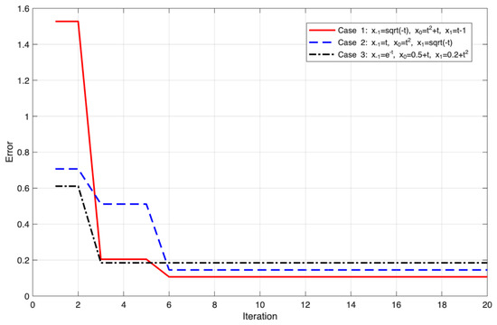
Figure 2 presents the evolution of the approximation error generated by the proposed algorithm for the three different initializations. It can be observed that the iterative sequence converges rapidly toward the common fixed point in all cases, indicating that the convergence behavior is robust with respect to the choice of initial functions. Furthermore, the error decreases significantly during the first few iterations and stabilizes afterward, providing numerical evidence supporting the strong convergence results established in the theoretical analysis.

Figure 2. Convergence behavior of the proposed SDITMA algorithm for three different initial function sets. The approximation error decreases rapidly and approaches a stable value within a few iterations, demonstrating the robustness of the algorithm with respect to different initializations.

Motivated by Lemma 3, we define the iterative mappings by $T_{1,k}=T_{2,k}:=P_{\mathcal{C}}(I-{\lambda }^{k}A)$, where $\left\{{\lambda }^k\right\}$ is a bounded positive sequence satisfying $\lim {\inf }_{k\to \infty }{\lambda }^k>0$. This construction allows the proposed shrinking double inertial Ishikawa-type algorithm to be applied to a monotone and Lipschitz continuous operator A in a Hilbert space.

4. Application in Extreme Learning Machine (ELM) to Air Quality Prediction

To evaluate the practical applicability and robustness of the proposed optimization algorithm, experiments were conducted using the Air Quality dataset obtained from the UCI Machine Learning Repository [28]. This dataset contains multivariate environmental measurements collected from air quality monitoring sensors, including pollutant concentrations and meteorological variables. The dataset is widely recognized as a benchmark dataset for regression and prediction tasks in environmental intelligence systems. The dataset was originally introduced by Vito et al. and is publicly available through the UCI Machine Learning Repository [28]. Recent studies have demonstrated that machine learning techniques, including deep learning, ensemble learning, and hybrid optimization methods, have substantially improved the accuracy of air quality prediction by effectively modeling nonlinear relationships among environmental variables [29,30].

Prior to model development, a comprehensive preprocessing procedure was performed to improve data quality and ensure the reliability of the subsequent learning process. Invalid sensor readings represented by the value $-200$ were treated as missing observations according to the dataset documentation. These missing values were subsequently handled using the K-Nearest Neighbor (KNN) imputation method with $k=5$. In addition, irrelevant columns were removed, duplicate observations were checked, and temporal variables were converted into datetime format to facilitate temporal analysis. The overview of dataset after preprocessing was shown in Table 1.

Table 1. Overview of dataset after preprocessing.

Variable	Data Type	Missing	Mean	Std	Min	Max
Date	datetime	0	–	–	–	–
Time	object	0	–	–	–	–
CO(GT)	float	0	2.087	1.417	0.100	11.900
PT08.S1(CO)	float	0	1100.180	214.700	647.250	2039.750
NMHC(GT)	float	0	229.631	147.334	7.000	1189.000
PT08.S2(NMHC)	float	0	941.299	265.676	383.250	2214.000
NOx(GT)	float	0	234.040	205.655	2.000	1479.000
PT08.S3(NOx)	float	0	832.875	254.017	322.000	2682.750
NO2(GT)	float	0	108.870	47.107	2.000	339.700
PT08.S4(NO2)	float	0	1456.681	341.948	551.000	2775.000
PT08.S5(O3)	float	0	1025.619	394.893	221.000	2522.750
T	float	0	18.376	8.715	−1.900	44.600
RH	float	0	49.166	17.083	9.175	88.725
AH	float	0	1.025	0.397	0.185	2.231

After preprocessing, the cleaned dataset was utilized to construct the Extreme Learning Machine (ELM) framework [31,32]. The proposed algorithm was then incorporated into the optimization stage of the ELM model in order to improve the estimation of output weights and enhance predictive performance. The integration of the proposed mathematical optimization mechanism with ELM enables efficient learning while maintaining strong generalization capability for air quality prediction tasks.

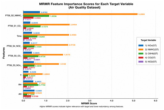
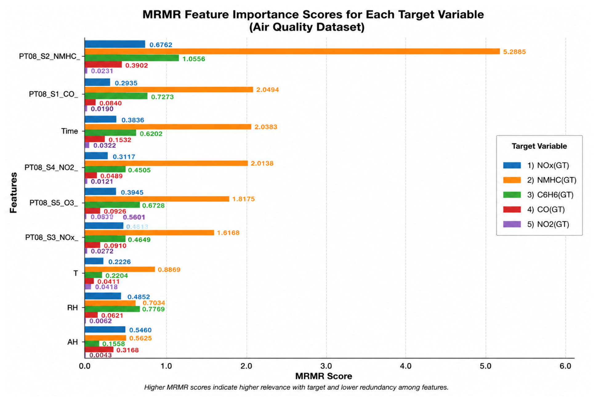
To investigate the relative contribution of environmental and sensor-based variables to air pollutant prediction, feature importance analysis was performed using the Minimum Redundancy Maximum Relevance (MRMR) algorithm implemented in the Regression Learner application of MATLAB R2025a. The MRMR method was employed to identify the most informative predictors while simultaneously minimizing redundancy among features. This analysis provides insight into the dominant variables influencing each target pollutant and supports the construction of a more efficient and generalized Extreme Learning Machine (ELM) framework. Figure 3 presents the comparative MRMR feature importance scores for multiple target variables in the Air Quality dataset.

Figure 3. Comparative visualization of MRMR-based feature importance scores across five air pollutant prediction targets in the Air Quality dataset, highlighting the relative contribution of sensor-based and meteorological variables.

To evaluate the effectiveness of the proposed ELM-based prediction framework under different feature configurations, multiple experimental cases were designed based on the MRMR feature selection results. The experiments considered both compact feature subsets consisting of the highest-ranked variables and full feature subsets containing all MRMR-selected variables. Recent studies have shown that feature selection remains an important preprocessing step for improving prediction performance, reducing redundancy, and enhancing model interpretability in environmental applications [33,34]. This strategy enables the investigation of the trade-off between model complexity and predictive performance across different air pollutant prediction tasks. Table 2 summarizes the experimental cases and feature selection settings used for each target variable.

Table 2. Experimental cases and feature selection strategies for each target variable.

Target Variable	Case	Feature Selection Strategy	Number of Features
NOx(GT)	Case 1	Top-5 MRMR-selected features	5
	Case 2	All MRMR-selected features	9
NMHC(GT)	Case 1	All MRMR-selected features	9
C6H6(GT)	Case 1	All MRMR-selected features	9
CO(GT)	Case 1	Top-5 MRMR-selected features	5
	Case 2	All MRMR-selected features	9
NO2(GT)	Case 1	Top-6 MRMR-selected features	6
	Case 2	All MRMR-selected features	9

To evaluate the predictive capability of the proposed iterative frameworks, Extreme Learning Machine (ELM) was employed as the regression model for air quality prediction. ELM is a single hidden-layer feedforward neural network characterized by fast learning speed and strong generalization performance. Unlike conventional neural networks, the input weights and hidden-layer biases are randomly assigned, while the output weights are analytically determined using optimization procedures. Recent developments have further extended ELM through regularization, metaheuristic optimization, and hybrid learning frameworks to improve prediction accuracy and robustness [35]. Due to its computational efficiency and reduced training complexity, ELM has become a practical approach for handling nonlinear prediction problems involving environmental and air quality datasets. In this study, the proposed iterative algorithms were incorporated into the ELM learning process to enhance the optimization of output parameters and improve predictive performance. The output of the single hidden-layer feedforward neural network (SLFN) for the i-th input sample is expressed as

$${\widehat{y}}_i={\displaystyle \sum _{j=1}^M}{w}_j\mathcal{A}(⟨a_j,x_i⟩+b_j),$$

(17)

where $\mathcal{A}(·)$ denotes the activation function, $a_j$ represents the input weight vector connecting the input layer to the j-th hidden node, $b_j$ is the bias of the j-th hidden node, and $w_j$ denotes the output weight associated with the corresponding hidden node.

The hidden layer output matrix $H\in {\mathbb{R}}^{N\times M}$ is constructed as The hidden layer output matrix $\mathcal{H}\in {\mathbb{R}}^{N\times M}$ is constructed as follows:

$$H=\left[\begin{array}{ccc}\mathcal{A}(⟨a_1,x_1⟩+b_1)& \dots & \mathcal{A}(⟨a_M,x_1⟩+b_M)\\ ⋮& \ddots & ⋮\\ \mathcal{A}(⟨a_1,x_N⟩+b_1)& \dots & \mathcal{A}(⟨a_M,x_N⟩+b_M)\end{array}\right].$$

Given the target vector $Y={[y_1,y_2,\dots ,y_N]}^T$, the output weight vector $w={[w_1,w_2,\dots ,w_M]}^T$ is obtained by solving $Hw=Y$.

Conventionally, the solution can be obtained using the Moore–Penrose pseudoinverse. However, for large-scale prediction problems, direct computation may become computationally expensive and may suffer from numerical instability. Instead of introducing an explicit regularization term, the learning process can be reformulated as a constrained least-squares optimization problem over a closed convex set $\mathcal{C}$:

$$\underset{w\in \mathcal{C}}{\min }{\displaystyle \frac{1}{2}}{\parallel Hw-Y\parallel }_2^2$$

(18)

where $\mathcal{C}\subseteq {\mathbb{R}}^M$ denotes a nonempty closed convex constraint set imposed on the output weights. The constraint set is introduced to ensure feasibility and improve the stability of the obtained solution while preserving desirable geometric properties in Hilbert spaces. For the ELM optimization problem, the iterative variable is identified with the output-weight vector, i.e.,

$$x_k=w_k.$$

Accordingly, the operator in the variational inequality formulation is defined by

$$A\left(w_k\right)=H^{\top }(H{w}_k-Y),$$

where H denotes the hidden-layer output matrix and Y is the target vector. Consequently, each iteration of Algorithms 2 and 3 updates the ELM output weights until convergence. The SDITMA framework is suitable for ELM training because estimating the output weights reduces to a convex least-squares problem, which can be formulated as a variational inequality involving the monotone and Lipschitz continuous operator. This structure is directly compatible with the projected gradient and extragradient constructions developed in the proposed framework. Moreover, the use of inertial extrapolation provides flexibility in navigating ill-conditioned or highly correlated feature spaces, which frequently arise in hidden-layer representations.

Algorithm 2 Shrinking Double Inertial Two-steps Projected Gradient Algorithm

Initialization: Let $x_{-1},x_0,x_1\in \mathcal{H}$ be arbitrary. Let $\left\{{\lambda }^k\right\}\subset (0,\infty )$ be bounded with $0<c\le {\lambda }^k\le d<{\displaystyle \frac{1}{L}}$, and let ${\theta }_k,{\delta }_k\in \mathbb{R}$ and ${\alpha }_k,{\beta }_k\in (0,1)$ for all $k\ge 1$. Set ${\mathcal{C}}_1=\mathcal{C}$,     Step 1. Compute the double inertial extrapolation $$y_k=x_k+{\nabla }_k,$$ where $${\nabla }_k={\theta }_k(x_k-x_{k-1})+{\delta }_k(x_{k-1}-x_{k-2}).$$     Step 2. Compute the first Ishikawa-type step $$z_k=(1-{\alpha }_k)y_k+{\alpha }_k{P}_{\mathcal{C}}(I-{\lambda }^{k}A)y_k.$$     Step 3. Compute the second Ishikawa-type step $$t_k=(1-{\beta }_k)z_k+{\beta }_k{P}_{\mathcal{C}}(I-{\lambda }^{k}A)z_k.$$     Step 4. Define the shrinking projection set $${\mathcal{C}}_{k+1}=\left\{u\in {\mathcal{C}}_k:\parallel t_k{-u\parallel }^2\le \parallel x_k{-u\parallel }^2+2⟨{\nabla }_k,x_k-u⟩+{\parallel {\nabla }_k\parallel }^2\right\}.$$     Step 5. Compute $$x_{k+1}=P_{{\mathcal{C}}_{k+1}}{x}_0.$$     Update $k:=k+1$ and return to Step 1.     Motivated by Lemma 4, we define the iterative mappings by $$T_{1,k}=T_{2,k}:=P_{\mathcal{C}}\left(I-{\lambda }^{k}A{P}_{\mathcal{C}}(I-{\lambda }^{k}A)\right),$$ where $\left\{{\lambda }^k\right\}\subset (0,\infty )$ satisfies $0<c\le {\lambda }^k\le d<{\displaystyle \frac{1}{L}}$. This construction incorporates a projected-gradient correction mechanism into the shrinking double inertial two-step framework and enables the proposed method to be applied to monotone and L-Lipschitz continuous operators in Hilbert spaces while preserving strong convergence properties.

Algorithm 3 Shrinking Double Inertial Two-steps Extragradient Algorithm

Initialization: Let $x_{-1},x_0,x_1\in \mathcal{H}$ be arbitrary. Let $0<c\le {\lambda }^k\le d<{\displaystyle \frac{1}{L}}$, and let ${\theta }_k,{\delta }_k\in \mathbb{R}$, ${\alpha }_k,{\beta }_k\in (0,1)$, for all $k\ge 1$. Set ${\mathcal{C}}_1=\mathcal{C}$.     Step 1. Compute the double inertial extrapolation $$y_k=x_k+{\nabla }_k,$$ where $${\nabla }_k={\theta }_k(x_k-x_{k-1})+{\delta }_k(x_{k-1}-x_{k-2}).$$     Step 2. Compute the first projected-gradient step $$z_k=(1-{\alpha }_k)y_k+{\alpha }_k{P}_{\mathcal{C}}\left(I-{\lambda }^{k}A{P}_{\mathcal{C}}(I-{\lambda }^{k}A)\right)y_k.$$     Step 3. Compute the second projected-gradient step $$t_k=(1-{\beta }_k)z_k+{\beta }_k{P}_{\mathcal{C}}\left(I-{\lambda }^{k}A{P}_{\mathcal{C}}(I-{\lambda }^{k}A)\right)z_k.$$     Step 4. Define the shrinking projection set $${\mathcal{C}}_{k+1}=\left\{u\in {\mathcal{C}}_k:\parallel t_k{-u\parallel }^2\le \parallel x_k{-u\parallel }^2+2⟨{\nabla }_k,x_k-u⟩+{\parallel {\nabla }_k\parallel }^2\right\}.$$     Step 5. Compute $$x_{k+1}=P_{{\mathcal{C}}_{k+1}}{x}_0.$$     Update $$k:=k+1$$ and return to Step 1.

To evaluate the regression performance of the predictive models, several commonly used metrics were employed, including the root mean square error (RMSE), mean absolute error (MAE) and coefficient of determination ($R^2$). These metrics provide complementary information regarding prediction accuracy and model generalization capability.

The RMSE is defined as

$$RMSE=\sqrt{{\displaystyle \frac{1}{N}}\sum _{i=1}^N{(y_i-{\widehat{y}}_i)}^2},$$

(19)

the MAE is computed by

$$MAE={\displaystyle \frac{1}{N}}{\displaystyle \sum _{i=1}^N}|y_i-{\widehat{y}}_i|,$$

(20)

and the coefficient of determination is given by

$$R^2=1-{\displaystyle \frac{{\sum }_{i=1}^N{(y_i-{\widehat{y}}_i)}^2}{{\sum }_{i=1}^N{(y_i-\overline{y})}^2}}.$$

(21)

Here, $y_i$, ${\widehat{y}}_i$, and $\overline{y}$ denote the observed value, predicted value, and mean observed value, respectively.

For all experiments, the proposed shrinking double inertial frameworks were combined with the ELM model under identical training and testing protocols to ensure a fair comparison. The parameters of the ELM model, including the number of hidden neurons, activation function, learning rate, and maximum number of iterations, were fixed throughout each experiment unless otherwise stated. The algorithm-specific parameters were selected empirically to achieve stable convergence and satisfactory predictive performance.

More specifically, the parameter settings used for the three proposed algorithms are summarized as follows:

Algorithm (3) (We note that Algorithm (3) refers to the algorithm presented in Equation (3)): ${\alpha }_k=0.9$ and ${\lambda }_k={\displaystyle \frac{0.999}{max\left(eig(A^T\ast A)\right)}}$

Algorithm 2, Algorithm 3: ${\alpha }_k=0.9$, ${\beta }_k=0.9$, ${\lambda }_k={\displaystyle \frac{0.999}{max\left(eig(A^T\ast A)\right)}}$

$$\begin{array}{c}\hfill {\theta }_k=\left\{\begin{array}{c}{\displaystyle \frac{1}{k\parallel x_k-x_{k-1}\parallel }},\mathrm{if}k>N,\hfill \\ 0.5,\mathrm{otherwise},\hfill \end{array}\right.\end{array}$$

and

$$\begin{array}{c}\hfill {\delta }_k=\left\{\begin{array}{c}{\displaystyle \frac{1}{k\parallel x_{k-1}-x_{k-2}\parallel }},\mathrm{if}k>N,\hfill \\ -0.1,\mathrm{otherwise}.\hfill \end{array}\right.\end{array}$$

In this example, $C=1$ denotes the unit ball: $C=\{x\in \mathcal{H}:\parallel x{\parallel }_2\le 1\}$.

To comprehensively evaluate the effectiveness of the proposed shrinking double inertial frameworks, experiments were conducted on five air quality target variables, namely, NOx(GT), NMHC(GT), C₆H₆(GT), CO(GT), and NO₂(GT). As summarized in Table 2, different feature selection strategies were considered for each target variable, including MRMR-selected subsets and the complete feature set. For each experimental case, the proposed algorithms were integrated with the Extreme Learning Machine (ELM) and evaluated under different constraint settings. Model performance was assessed using five-fold cross-validation and an independent test set based on RMSE, MAE, and the coefficient of determination ($R^2$). The complete dataset was randomly divided into two subsets using a hold-out strategy. Specifically, 90% of the observations were used for model development, while the remaining 10% were reserved as an independent test set. The training subset was further evaluated using five-fold cross-validation. In each fold, four subsets were used for training and one subset for validation. After cross-validation, the final model was retrained using the entire 90% training dataset and evaluated on the independent test set. To ensure reproducibility, all experiments were conducted using a fixed random seed (rng(42) in MATLAB ), which controlled both the data partitioning and the random initialization of the ELM parameters. Before model training, all predictor variables were standardized using Z-score normalization. The mean and standard deviation were computed exclusively from the training dataset and subsequently applied to the validation and independent test datasets to avoid information leakage. Similarly, the target variable was standardized during model training and transformed back to its original scale before performance evaluation. The ELM model consisted of a single hidden layer containing 100 hidden neurons. The rectified linear unit (ReLU) activation function was adopted for all experiments, and is defined by

$$g\left(z\right)=\max (0,z).$$

The hidden-layer parameters were randomly initialized and remained fixed throughout the learning process, whereas the output weights were updated using the proposed optimization algorithms. The maximum number of training epochs was fixed at 1000 for all experiments. The learning rate was set to 0.01, while the mini-batch size was 64. The comparative results for the five target variables are presented in the following tables.

The prediction performance under $C=\mathcal{H}$ and $C=1$ was identical because the projection operator was inactive throughout the iterations. Therefore, only the representative results under $C=\mathcal{H}$ are presented.

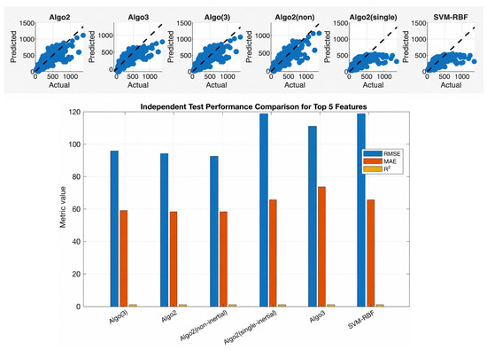
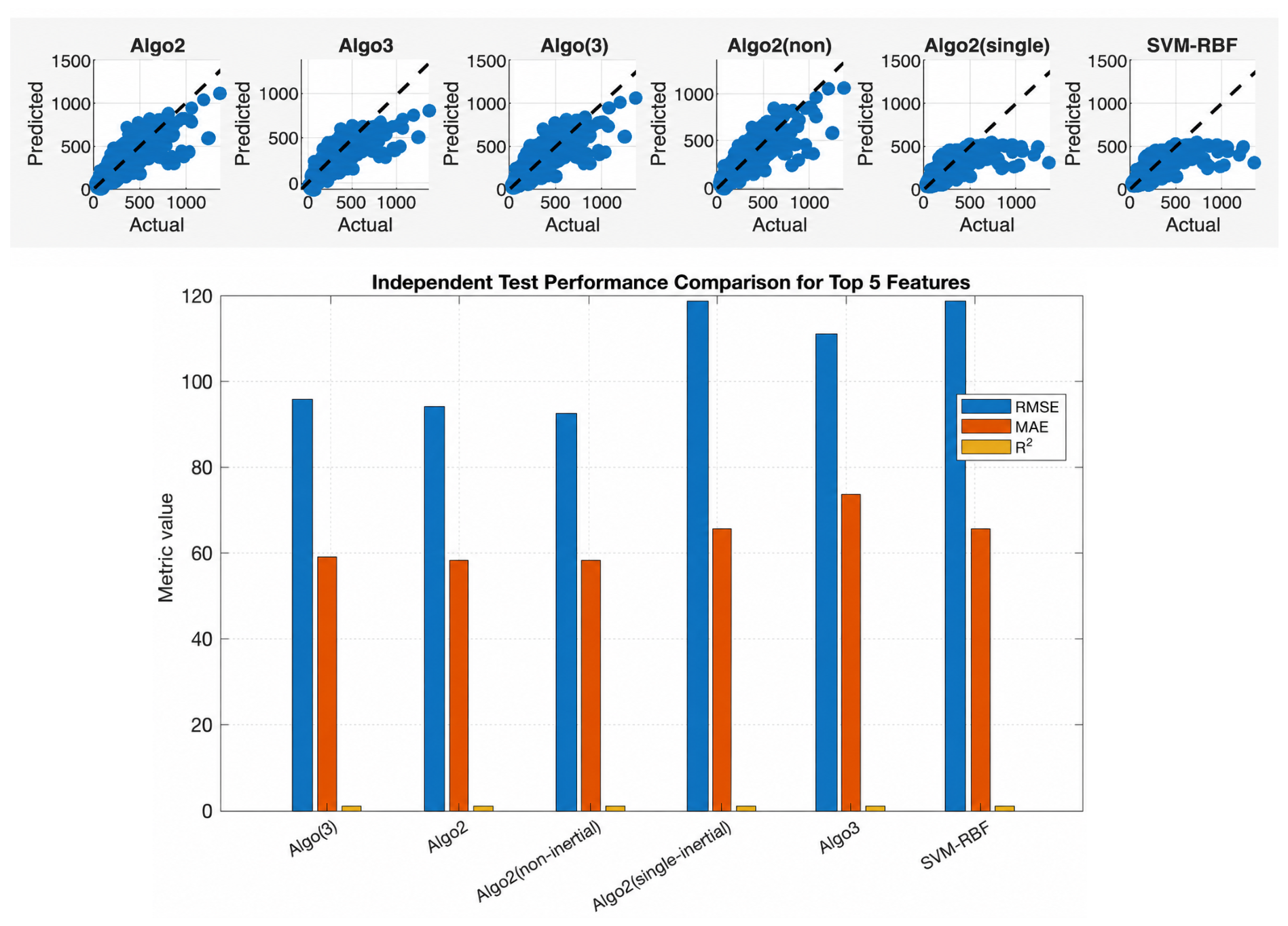
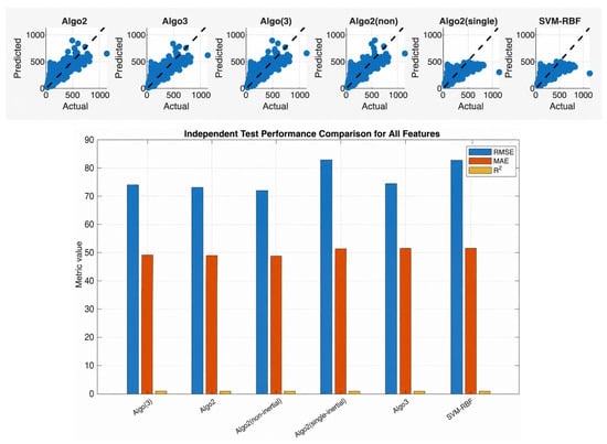
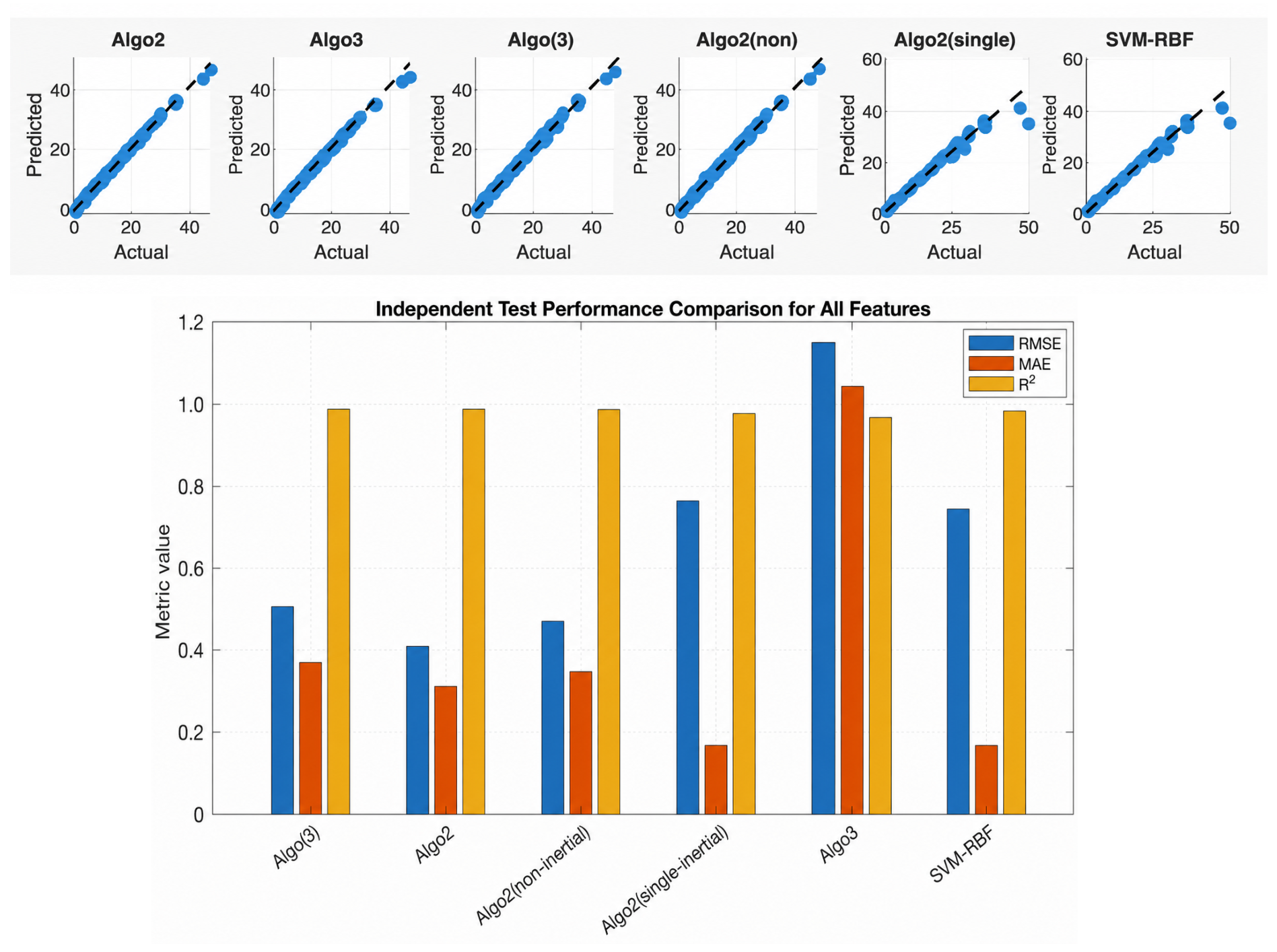
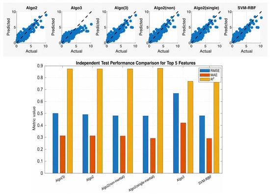
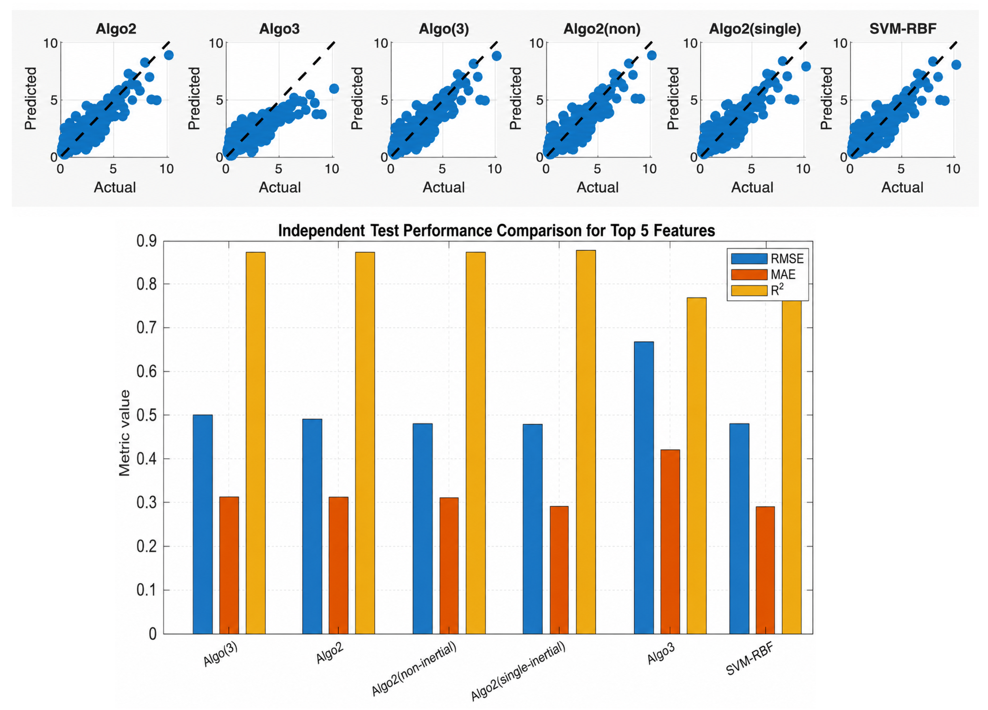
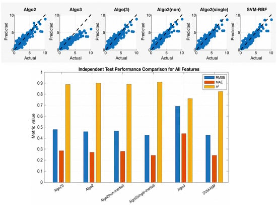
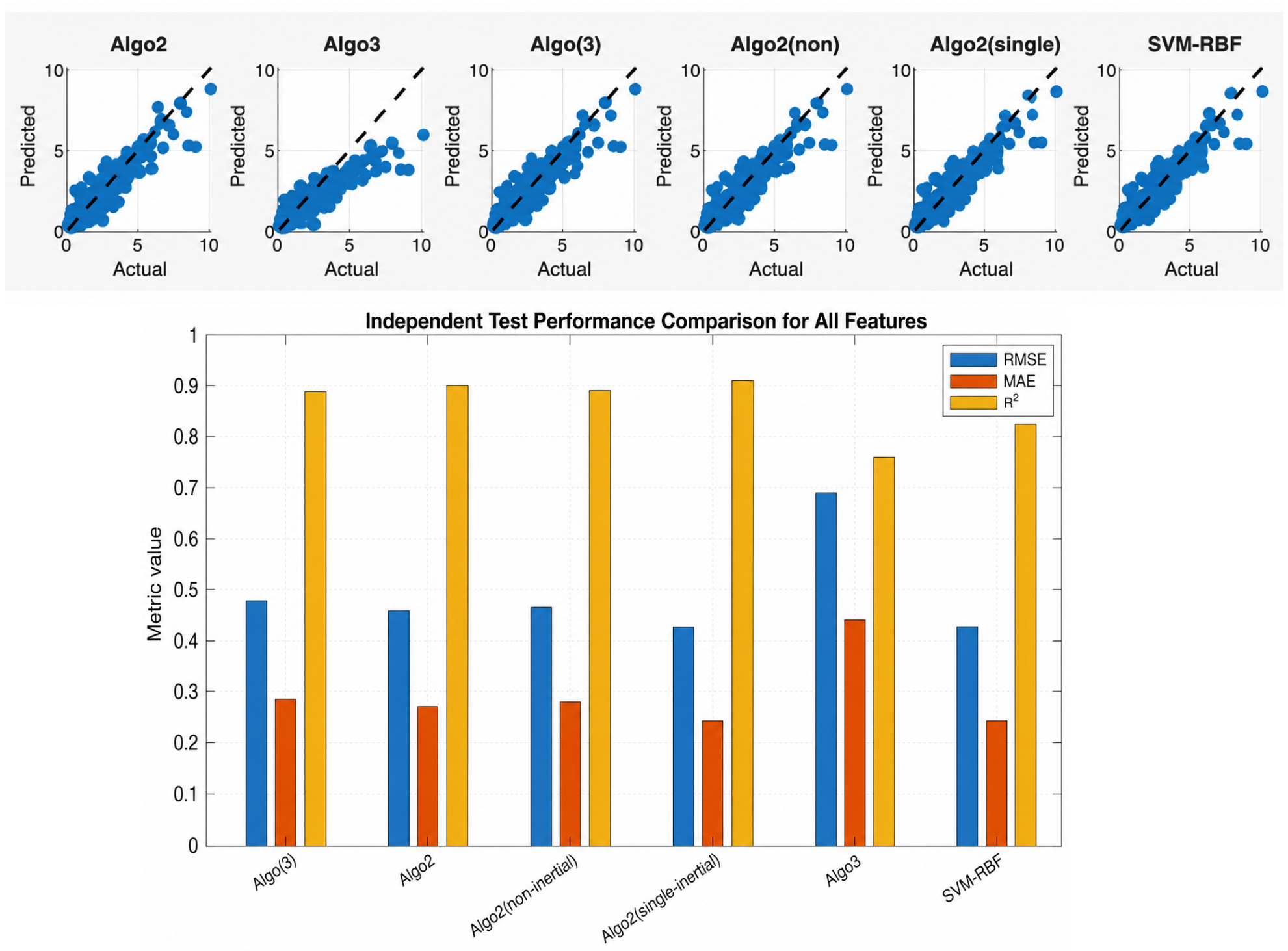
From Table 3 and Figure 4 and Figure 5, Algo 2 (non-inertial) consistently achieved the best cross-validation performance under both feature configurations. For the Top 5 feature set, it also produced the best test performance across all evaluation metrics. Under the All Features setting, the proposed double-inertial Algo 2 achieved a slightly lower test RMSE and higher test $R^2$, while the non-inertial variant attained the lowest test MAE.

Table 3. Performance comparison for NOx(GT) prediction using ELM with ReLU activation. Cross-validation results are reported as mean ± standard deviation. The numerical results under $C=\mathcal{H}$ and $C=1$ were identical.

Feature Set	Constraint	Algorithm	CV RMSE	CV MAE	CV ${\mathit{R}}^2$	Test RMSE	Test MAE	Test ${\mathit{R}}^2$
Top 5	$C=\mathcal{H}$ and $C=1$ (identical)	Algo 2	$90.547\pm 2.159$	$59.199\pm 0.574$	$0.80671\pm 0.00830$	94.270	58.533	0.78136
		Algo 3	$98.740\pm 7.149$	$65.202\pm 6.024$	$0.76968\pm 0.02920$	111.640	74.006	0.69339
		Algo (3)	$91.564\pm 2.030$	$59.737\pm 0.945$	$0.80237\pm 0.00729$	95.964	58.970	0.77344
		Algo 2 (non-inertial)	$88.686\pm 2.145$	$58.549\pm 0.859$	$0.81447\pm 0.01062$	$92.904$	$58.403$	$0.78766$
		Algo 2 (single-inertial)	$125.510\pm 4.859$	$71.835\pm 2.333$	$0.62869\pm 0.02047$	119.120	65.526	0.65091
		SVM-RBF	$126.440\pm 5.353$	$72.102\pm 2.559$	$0.62329\pm 0.02134$	119.310	65.592	0.64977
All Features	$C=\mathcal{H}$ and $C=1$ (identical)	Algo 2	$71.060\pm 4.355$	$45.181\pm 1.015$	$0.88063\pm 0.01462$	$71.808$	45.745	$0.87314$
		Algo 3	$72.448\pm 4.130$	$46.851\pm 2.480$	$0.87603\pm 0.01355$	105.230	68.466	0.72756
		Algo (3)	$72.299\pm 3.990$	$46.156\pm 1.311$	$0.87648\pm 0.01387$	73.907	45.929	0.86562
		Algo 2 (non-inertial)	$69.261\pm 4.055$	$44.885\pm 1.331$	$0.88663\pm 0.01318$	71.884	$45.214$	0.87287
		Algo 2 (single-inertial)	$131.770\pm 5.681$	$71.655\pm 2.936$	$0.59079\pm 0.02408$	124.400	64.672	0.61928
		SVM-RBF	$132.490\pm 5.048$	$71.957\pm 2.686$	$0.58637\pm 0.02017$	123.630	64.332	0.62395

Figure 4. Predictionperformance of NOx(GT) using the Top-5 MRMR-selected features with ReLU activation under $C=\mathcal{H}$, showing predictive accuracy and test performance (RMSE, MAE, and $R^2$).

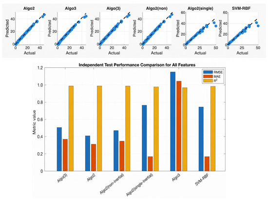
Figure 5. Prediction performance of NOx(GT) using all MRMR-selected features with ReLU activation under $C=\mathcal{H}$, showing actual-versus-predicted relationships and test performance (RMSE, MAE, and $R^2$).

The prediction performance under $C=\mathcal{H}$ and $C=1$ was identical because the projection operator was inactive throughout the iterations. Therefore, only the representative results under $C=\mathcal{H}$ are presented.

The results in Table 4 and Figure 6 indicate that Algo 2 (non-inertial) consistently achieved the best overall performance, yielding the lowest cross-validation RMSE, the highest cross-validation $R^2$, and the best test performance in terms of RMSE, MAE, and $R^2$. Although the proposed double-inertial Algo 2 obtained the lowest cross-validation MAE, its overall performance was slightly inferior to the non-inertial variant.

Table 4. Performance comparison for NMHC(GT) prediction using ELM with ReLU activation. Cross-validation results are reported as mean ± standard deviation. The numerical results under $C=\mathcal{H}$ and $C=1$ were identical.

Feature Set	Constraint	Algorithm	CV RMSE	CV MAE	CV ${\mathit{R}}^2$	Test RMSE	Test MAE	Test ${\mathit{R}}^2$
All Features	$C=\mathcal{H}$ and $C=1$ (identical)	Algo 2	$72.502\pm 1.954$	$49.503\pm 0.852$	$0.76017\pm 0.00588$	73.427	48.700	0.72393
		Algo 3	$78.129\pm 7.983$	$54.512\pm 7.095$	$0.71945\pm 0.05690$	74.511	51.147	0.71572
		Algo (3)	$73.882\pm 2.576$	$49.852\pm 1.326$	$0.75098\pm 0.00884$	74.007	49.134	0.71955
		Algo 2 (non-inertial)	$71.736\pm 1.254$	$49.737\pm 1.063$	$0.76515\pm 0.00473$	$72.228$	$48.613$	$0.73287$
		Algo 2 (single-inertial)	$89.567\pm 3.969$	$57.041\pm 2.076$	$0.63407\pm 0.01795$	83.070	51.336	0.64666
		SVM-RBF	$89.969\pm 4.307$	$57.196\pm 2.145$	$0.63079\pm 0.02025$	82.818	51.278	0.64880

Figure 6. Prediction performance of NMHC(GT) using all MRMR-selected features with ReLU activation under $C=\mathcal{H}$, showing actual-versus-predicted relationships and test performance (RMSE, MAE, and $R^2$).

The prediction performance under $C=\mathcal{H}$ and $C=1$ was identical because the projection operator was inactive throughout the iterations. Therefore, only the representative results under $C=\mathcal{H}$ are presented.

The results presented in Table 5 and Figure 7 demonstrate that the proposed Algo 2 (double-inertial) achieved the best overall performance, yielding the lowest cross-validation RMSE, the highest cross-validation $R^2$, and the best test performance in terms of RMSE, MAE, and $R^2$. Although the non-inertial variant obtained the lowest cross-validation MAE, its overall predictive performance was slightly inferior to the proposed method.

Table 5. Performance comparison for C₆H₆(GT) prediction using ELM with ReLU activation. Cross-validation results are reported as mean ± standard deviation. The numerical results under $C=\mathcal{H}$ and $C=1$ were identical.

Feature Set	Constraint	Algorithm	CV RMSE	CV MAE	CV ${\mathit{R}}^2$	Test RMSE	Test MAE	Test ${\mathit{R}}^2$
All Features	$C=\mathcal{H}$ and $C=1$ (identical)	Algo 2	$0.44607\pm 0.06175$	$0.31709\pm 0.03846$	$0.99636\pm 0.00093$	$0.40986$	$0.31208$	$0.99672$
		Algo 3	$1.31570\pm 0.93441$	$0.89158\pm 0.57959$	$0.95623\pm 0.05825$	1.16220	1.04430	0.97362
		Algo (3)	$0.55987\pm 0.05559$	$0.38488\pm 0.02930$	$0.99431\pm 0.00110$	0.51379	0.36912	0.99484
		Algo 2 (non-inertial)	$0.44978\pm 0.06730$	$0.31525\pm 0.01885$	$0.99631\pm 0.00109$	0.47218	0.34904	0.99565
		Algo 2 (single-inertial)	$0.98466\pm 0.23846$	$0.21312\pm 0.01805$	$0.98179\pm 0.00889$	0.76573	0.17486	0.98855
		SVM-RBF	$1.00700\pm 0.26096$	$0.21765\pm 0.02127$	$0.98086\pm 0.01016$	0.74911	0.17199	0.98904

Figure 7. Prediction performance of C₆H₆(GT) using all MRMR-selected features with ReLU activation under $C=\mathcal{H}$, showing prediction accuracy and test metrics (RMSE, MAE, and $R^2$).

The prediction performance under $C=\mathcal{H}$ and $C=1$ was identical because the projection operator was inactive throughout the iterations. Therefore, only the representative results under $C=\mathcal{H}$ are presented.

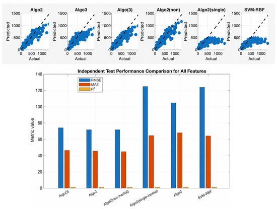
The numerical results in Table 6 and Figure 8 and Figure 9 indicate that SVM-RBF achieved the best cross-validation performance under both the Top 5 and All Features settings. However, Algo 2 (single-inertial) consistently produced the best test performance, yielding the lowest test RMSE and MAE together with the highest test $R^2$. The proposed double-inertial and non-inertial variants remained competitive but did not surpass the single-inertial variant on the independent test set. These findings indicate that the single-inertial framework provides the strongest generalization performance for CO(GT) prediction among the evaluated methods.

Table 6. Performance comparison for CO(GT) prediction using ELM with Tanh activation. Cross-validation results are reported as mean ± standard deviation. The numerical results under $C=\mathcal{H}$ and $C=1$ were identical.

Feature Set	Constraint	Algorithm	CV RMSE	CV MAE	CV ${\mathit{R}}^2$	Test RMSE	Test MAE	Test ${\mathit{R}}^2$
Top 5	$C=\mathcal{H}$ and $C=1$ (identical)	Algo 2	$0.47913\pm 0.04481$	$0.31270\pm 0.03214$	$0.88472\pm 0.02270$	0.49325	0.30920	0.87971
		Algo 3	$0.74326\pm 0.21011$	$0.48773\pm 0.12638$	$0.70588\pm 0.16788$	0.67388	0.42224	0.77547
		Algo (3)	$0.46229\pm 0.01182$	$0.30334\pm 0.00392$	$0.89333\pm 0.00690$	0.49850	0.31150	0.87713
		Algo 2 (non-inertial)	$0.45292\pm 0.01495$	$0.29806\pm 0.00311$	$0.89756\pm 0.00816$	0.48437	0.30928	0.88400
		Algo 2 (single-inertial)	$0.44217\pm 0.01108$	$0.28020\pm 0.00484$	$0.90242\pm 0.00611$	0.47968	0.29248	0.88623
		SVM-RBF	$0.44113\pm 0.01044$	$0.27976\pm 0.00456$	$0.90289\pm 0.00579$	0.48264	0.29423	0.88482
All Features	$C=\mathcal{H}$ and $C=1$ (identical)	Algo 2	$0.43124\pm 0.01536$	$0.27310\pm 0.00212$	$0.90713\pm 0.00768$	0.45718	0.27077	0.89665
		Algo 3	$0.55281\pm 0.10085$	$0.35446\pm 0.06910$	$0.84346\pm 0.05448$	0.68959	0.44041	0.76488
		Algo (3)	$0.43504\pm 0.01512$	$0.27636\pm 0.00230$	$0.90548\pm 0.00778$	0.47791	0.28252	0.88707
		Algo 2 (non-inertial)	$0.42213\pm 0.01361$	$0.27035\pm 0.00410$	$0.91103\pm 0.00667$	0.46556	0.28101	0.89283
		Algo 2 (single-inertial)	$0.40103\pm 0.00968$	$0.24163\pm 0.00236$	$0.91974\pm 0.00483$	0.42927	0.24222	0.90889
		SVM-RBF	$0.40002\pm 0.01072$	$0.24119\pm 0.00231$	$0.92014\pm 0.00525$	0.43011	0.24248	0.90853

Figure 8. Prediction performance of CO(GT) using the Top-5 MRMR-selected features with Tanh activation under $C=\mathcal{H}$, showing prediction accuracy and test metrics (RMSE, MAE, and $R^2$).

Figure 9. Prediction performance of CO(GT) using all MRMR-selected features with Tanh activation under $C=\mathcal{H}$, showing prediction accuracy and test metrics (RMSE, MAE, and $R^2$).

The prediction performance under $C=\mathcal{H}$ and $C=1$ was identical because the projection operator was inactive throughout the iterations. Therefore, only the representative results under $C=\mathcal{H}$ are presented.

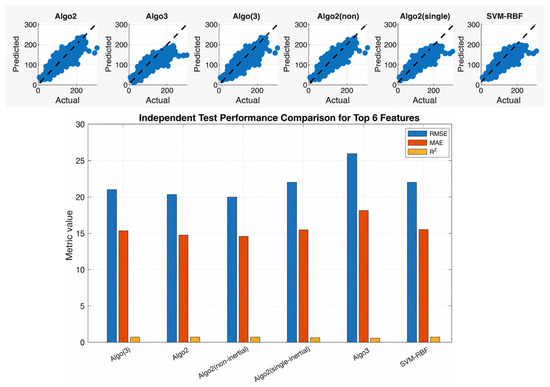
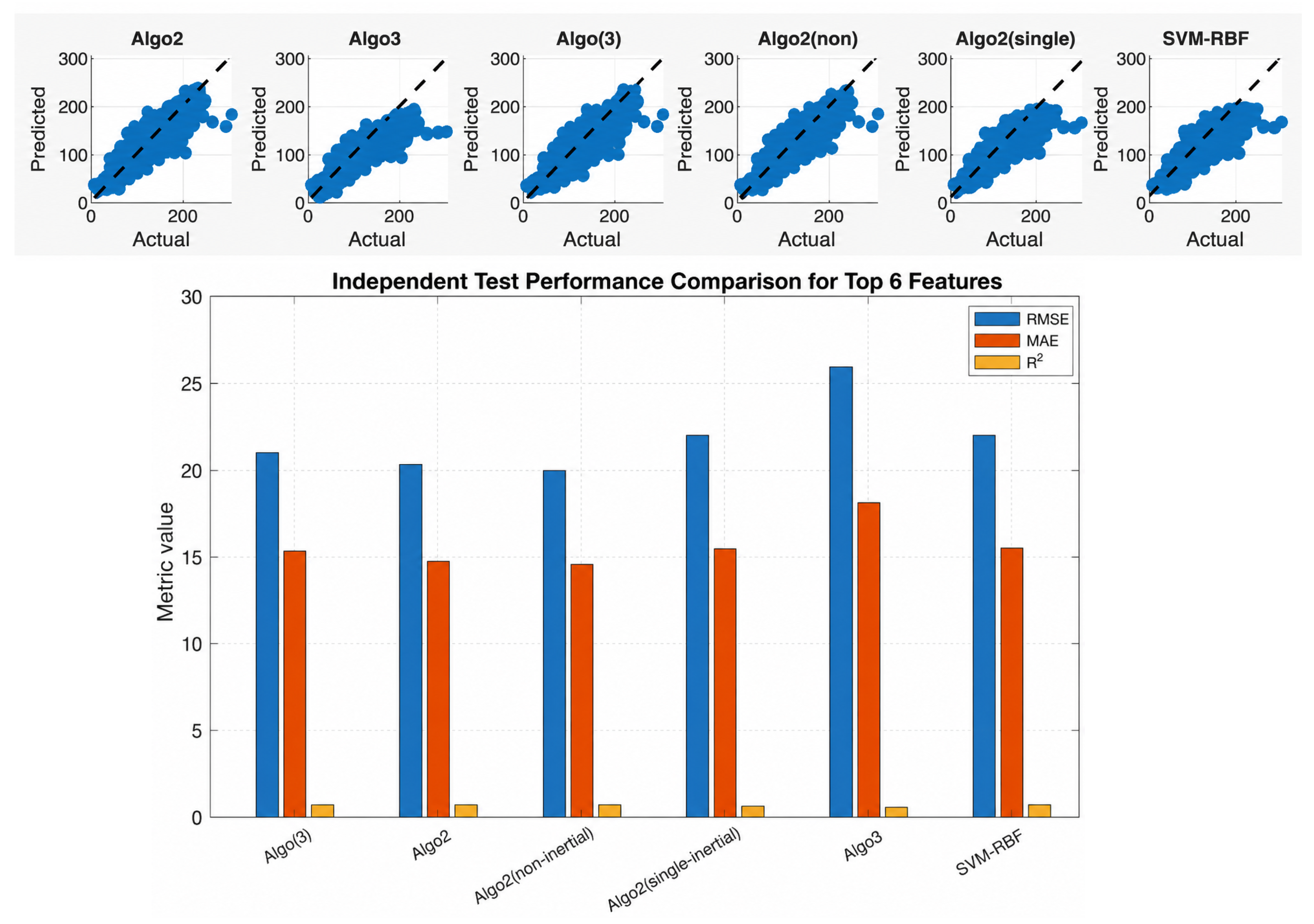
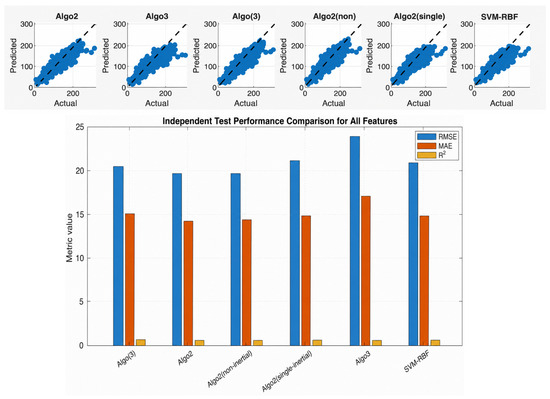
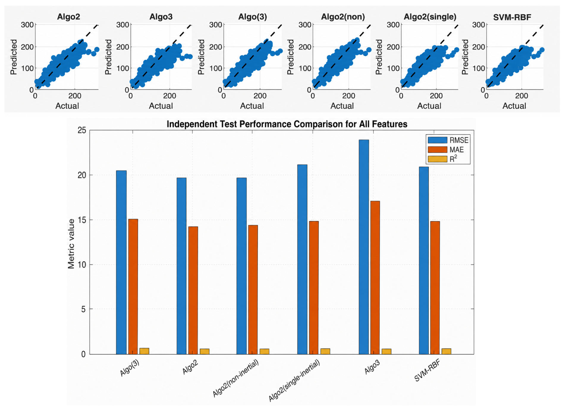
The numerical results in Table 7 and Figure 10 and Figure 11 indicate that Algo 2 (non-inertial) achieved the best cross-validation performance under both the Top 6 and All Features settings. For the Top 6 feature set, it also produced the best test performance across all evaluation metrics. Under the All Features configuration, the proposed Algo 2 (double-inertial) achieved a marginally lower test RMSE, the lowest test MAE, and the highest test $R^2$, although its performance was very close to that of the non-inertial variant. Overall, both the double-inertial and non-inertial algorithms outperformed Algo 3, Algo (3), the single-inertial variant, and the SVM-RBF baseline for NO₂(GT) prediction.

Table 7. Performance comparison for NO₂(GT) prediction using ELM with Tanh activation. Cross-validation results are reported as mean ± standard deviation. The numerical results under $C=\mathcal{H}$ and $C=1$ were identical.

Feature Set	Constraint	Algorithm	CV RMSE	CV MAE	CV ${\mathit{R}}^2$	Test RMSE	Test MAE	Test ${\mathit{R}}^2$
Top 6	$C=\mathcal{H}$ and $C=1$ (identical)	Algo 2	$21.445\pm 0.687$	$15.569\pm 0.465$	$0.79174\pm 0.01351$	20.423	14.766	0.81682
		Algo 3	$23.718\pm 2.568$	$17.282\pm 1.920$	$0.74281\pm 0.05707$	26.117	18.201	0.70044
		Algo (3)	$21.981\pm 0.914$	$16.005\pm 0.768$	$0.78113\pm 0.01742$	21.070	15.333	0.80502
		Algo 2 (non-inertial)	$21.164\pm 0.674$	$15.421\pm 0.516$	$0.79718\pm 0.01281$	$19.997$	$14.537$	$0.82437$
		Algo 2 (single-inertial)	$23.290\pm 0.556$	$16.417\pm 0.392$	$0.75455\pm 0.00907$	22.194	15.559	0.78368
		SVM-RBF	$23.334\pm 0.581$	$16.408\pm 0.391$	$0.75363\pm 0.00915$	22.164	15.602	0.78425
All Features	$C=\mathcal{H}$ and $C=1$ (identical)	Algo 2	$20.374\pm 0.644$	$14.676\pm 0.544$	$0.81204\pm 0.01189$	$19.647$	$14.259$	$0.83048$
		Algo 3	$22.668\pm 1.748$	$16.465\pm 1.471$	$0.76659\pm 0.03383$	24.182	17.172	0.74318
		Algo (3)	$20.715\pm 0.504$	$14.921\pm 0.380$	$0.80573\pm 0.00985$	20.455	15.021	0.81624
		Algo 2 (non-inertial)	$20.339\pm 0.276$	$14.678\pm 0.234$	$0.81278\pm 0.00589$	19.650	14.367	0.83043
		Algo 2 (single-inertial)	$22.518\pm 0.590$	$15.598\pm 0.415$	$0.77056\pm 0.00836$	21.171	14.792	0.80316
		SVM-RBF	$22.597\pm 0.583$	$15.618\pm 0.410$	$0.76894\pm 0.00864$	21.134	14.785	0.80384

Figure 10. Prediction performance of NO₂(GT) using the Top-6 MRMR-selected features with Tanh activation under $C=\mathcal{H}$, showing prediction accuracy and test metrics (RMSE, MAE, and $R^2$).

Figure 11. Prediction performance of NO₂(GT) using all MRMR-selected features with Tanh activation under $C=\mathcal{H}$, showing prediction accuracy and test metrics (RMSE, MAE, and $R^2$).

5. Discussion

The main contribution of this work is the development of a shrinking double inertial framework for solving common fixed point problems associated with a countable family of quasi-nonexpansive mappings. The proposed framework combines two complementary mechanisms. First, the shrinking projection strategy guarantees strong convergence of the generated sequence to a common fixed point. Second, the double inertial extrapolation incorporates information from multiple previous iterates, providing additional flexibility in the iterative process while preserving strong convergence.

The numerical example in an infinite-dimensional function space verifies the theoretical convergence analysis. In particular, the proposed framework remains applicable to quasi-nonexpansive mappings that are not necessarily nonexpansive, demonstrating a broader scope than many existing fixed-point methods. The convergence trajectories further indicate that the iterates approach the common fixed point reliably from different initializations, confirming the robustness of the proposed algorithms. Under the assumptions stated in the convergence theorems, including monotonicity and Lipschitz continuity of the operator and the prescribed conditions on the control parameters, the generated sequence $\left\{w_k\right\}$ converges strongly to a solution of the corresponding variational inequality. In the ELM setting, this means that the sequence of output-weight estimates converges in norm to a feasible least-squares solution. This theoretical result provides stability of the iterative training procedure and rules out divergence of the weight sequence under the stated assumptions. However, the convergence guarantee concerns optimization stability and does not by itself guarantee superior test-set generalization.

Building upon the fixed-point framework, Algorithms 2 and 3 were extended to solve variational inequality problems involving monotone and Lipschitz continuous operators. These formulations naturally integrate with the optimization of Extreme Learning Machines (ELMs), where the proposed algorithms are employed to estimate the output weights for air quality prediction.

The experimental results demonstrate that the most suitable inertial strategy depends on the prediction target rather than a single algorithm consistently outperforming all others. For NOx(GT), NMHC(GT), and NO₂(GT), the non-inertial variant of Algorithm 2 generally achieved the best cross-validation performance, and in most cases the best overall prediction accuracy. For C₆H₆(GT), the proposed double-inertial Algorithm 2 produced the best predictive performance, indicating that the additional inertial extrapolation can improve generalization for certain regression tasks. In contrast, for CO(GT) the single-inertial variant yielded the best test performance, although the SVM-RBF baseline achieved the highest cross-validation accuracy. These observations indicate that the effectiveness of the inertial mechanism is problem-dependent and is closely related to the characteristics of the target variable and the underlying data distribution.

Another important observation is that using all selected features generally improved predictive performance compared with reduced feature subsets, particularly for NOx(GT) and NO₂(GT). Moreover, the numerical results obtained under the unconstrained setting $C=\mathcal{H}$ and the unit-ball constraint $C=1$ were identical throughout all experiments. This occurs because the computed output-weight vector satisfies $\parallel \beta \parallel <1$ during the entire optimization process; consequently, the projection onto the unit ball remains inactive, that is,

$$P_C\left(\beta \right)=\beta ,$$

at every iteration. Therefore, both constraint settings generate identical iterative sequences and consequently produce identical prediction performance.

Overall, the experimental results suggest that the proposed shrinking double-inertial framework should be viewed as a flexible optimization family rather than a single universally superior algorithm. The double-inertial, single-inertial, and non-inertial variants exhibit complementary strengths across different pollutants; in particular, the proposed double-inertial strategy demonstrates an advantage for C₆H₆(GT) prediction, whereas the non-inertial and single-inertial variants provide superior performance for several other prediction tasks. This flexibility enables practitioners to select the most appropriate optimization strategy according to the characteristics of the target problem while retaining the same theoretical convergence guarantees established in this work.

Future work will consider extending the proposed framework to stochastic and adaptive inertial schemes, variable inertial parameter selection, nonconvex optimization, and large-scale deep learning architectures for environmental monitoring and healthcare prediction.

6. Conclusions

This paper proposes a shrinking double inertial framework for approximating common fixed points of a countable family of quasi-nonexpansive mappings in Hilbert spaces. By combining shrinking projection techniques with double inertial extrapolation, strong convergence of the generated sequence is established under suitable assumptions. A numerical example in an infinite-dimensional function space verifies the theoretical convergence results and demonstrates that the proposed framework remains applicable to quasi-nonexpansive mappings that are not necessarily nonexpansive.

Building upon the fixed-point framework, two variational inequality-based extensions are developed through projected gradient and extragradient constructions, enabling the proposed algorithms to solve optimization problems arising in machine learning. These methods are successfully applied to Extreme Learning Machines for predicting five air quality indicators: NOx(GT), NMHC(GT), C₆H₆(GT), CO(GT), and NO₂(GT). The experimental results show that no single inertial strategy consistently outperformed all others across every prediction target; instead, the double-inertial, single-inertial, and non-inertial variants exhibited complementary strengths depending on the characteristics of the pollutant and the underlying data distribution. In particular, the proposed double-inertial framework achieved the best predictive performance for C₆H₆(GT), whereas the non-inertial and single-inertial variants provided superior performance for several other prediction tasks.

Overall, the proposed framework provides a flexible family of optimization algorithms with rigorous convergence guarantees and competitive predictive performance across diverse air quality prediction problems. The theoretical developments together with the experimental results demonstrate that the proposed methodologies constitute an effective bridge between modern fixed-point theory, variational inequality methods, and data-driven machine learning applications.

Future work will consider adaptive inertial parameter selection, stochastic and nonconvex extensions, distributed and large-scale optimization, and applications to deep learning architectures for environmental monitoring and healthcare prediction.

References

- Bauschke, H.H.; Combettes, P.L. Convex Analysis and Monotone Operator Theory in Hilbert Spaces, 2nd ed.; Springer: Cham, Switzerland, 2017. [Google Scholar] [CrossRef] [Scilit]
- Combettes, P.L. The convex feasibility problem in image recovery. In Advances in Imaging and Electron Physics; Elsevier: Amsterdam, The Netherlands, 1996; Volume 95, pp. 155–270. [Google Scholar]
- Mann, W.R. Mean value methods in iteration. Proc. Am. Math. Soc. 1953, 4, 506–510. [Google Scholar] [CrossRef] [Scilit]
- Ishikawa, S. Fixed points by a new iteration method. Proc. Am. Math. Soc. 1974, 44, 147–150. [Google Scholar] [CrossRef]
- Marino, G.; Xu, H.K. Weak and strong convergence theorems for strict pseudo-contractions in Hilbert spaces. J. Math. Anal. Appl. 2007, 329, 336–346. [Google Scholar] [CrossRef] [Scilit]
- Schu, J. Iterative construction of fixed points of asymptotically nonexpansive mappings. J. Math. Anal. Appl. 1991, 158, 407–413. [Google Scholar] [CrossRef] [Scilit]
- Noor, M.A. New approximation schemes for general variational inequalities. J. Math. Anal. Appl. 2000, 251, 217–229. [Google Scholar] [CrossRef] [Scilit]
- Agarwal, R.P.; O’Regan, D.; Sahu, D.R. Iterative construction of fixed points of nearly asymptotically nonexpansive mappings. J. Nonlinear Convex Anal. 2007, 8, 61–79. Available online: http://www.ybook.co.jp/online-p/JNCA/vol8/jncav8n1p61.pdf?utm (accessed on 1 April 2026).
- Phuengrattana, W.; Suantai, S. On the rate of convergence of Mann, Ishikawa, Noor and SP-iterations for continuous functions on an arbitrary interval. J. Comput. Appl. Math. 2011, 235, 3006–3014. [Google Scholar] [CrossRef] [Scilit]
- Genel, A.; Lindenstrauss, J. An example concerning fixed points. Isr. J. Math. 1975, 22, 81–86. [Google Scholar] [CrossRef] [Scilit]
- Halpern, B. Fixed points of nonexpanding maps. Bull. Am. Math. Soc. 1967, 73, 957–961. [Google Scholar] [CrossRef] [Scilit]
- Nakajo, K.; Takahashi, W. Strong convergence theorems for nonexpansive mappings and nonexpansive semigroups. J. Math. Anal. Appl. 2003, 279, 372–379. [Google Scholar] [CrossRef] [Scilit]
- Takahashi, W.; Takeuchi, Y.; Kubota, R. Strong convergence theorems by hybrid methods for families of nonexpansive mappings in Hilbert spaces. J. Math. Anal. Appl. 2008, 341, 276–286. [Google Scholar] [CrossRef] [Scilit]
- Aoyama, K.; Kohsaka, F.; Takahashi, W. Shrinking projection methods for firmly nonexpansive mappings. Nonlinear Anal. Theory Methods Appl. 2009, 71, e1626–e1632. [Google Scholar] [CrossRef] [Scilit]
- Kondo, A. Strong convergence to common fixed points using Ishikawa and hybrid methods for mean-demiclosed mappings in Hilbert spaces. Math. Model. Anal. 2023, 28, 285–307. [Google Scholar] [CrossRef] [Scilit]
- Polyak, B.T. Some methods of speeding up the convergence of iteration methods. USSR Comput. Math. Math. Phys. 1964, 4, 1–17. [Google Scholar] [CrossRef] [Scilit]
- Alvarez, F.; Attouch, H. An inertial proximal method for maximal monotone operators via discretization of a nonlinear oscillator with damping. Set-Valued Anal. 2001, 9, 3–11. [Google Scholar] [CrossRef] [Scilit]
- Maingé, P.-E. Convergence theorems for inertial KM-type algorithms. J. Comput. Appl. Math. 2008, 219, 223–236. [Google Scholar] [CrossRef] [Scilit]
- Boţ, R.I.; Csetnek, E.R.; Hendrich, C. Inertial Douglas–Rachford splitting for monotone inclusion problems. Appl. Math. Comput. 2015, 256, 472–487. [Google Scholar] [CrossRef] [Scilit]
- Lorenz, D.A.; Pock, T. An inertial forward-backward algorithm for monotone inclusions. J. Math. Imaging Vis. 2015, 51, 311–325. [Google Scholar] [CrossRef] [Scilit]
- Dong, Q.L.; Yuan, H.B.; Cho, Y.J.; Rassias, T.M. Modified inertial Mann algorithm and inertial CQ-algorithm for nonexpansive mappings. Optim. Lett. 2018, 12, 87–102. [Google Scholar] [CrossRef] [Scilit]
- Iyiola, O.S.; Shehu, Y. New convergence results for inertial Krasnoselskii–Mann iterations in Hilbert spaces with applications. Results Math. 2022, 76, 75. [Google Scholar] [CrossRef] [Scilit]
- Hartman, P.; Stampacchia, G. On some non-linear elliptic differential-functional equations. Acta Math. 1966, 115, 271–310. [Google Scholar] [CrossRef] [Scilit]
- Cholamjiak, W. Fixed Point Optimization Algorithms and Their Applications; Morgan Kaufmann: Amsterdam, The Netherlands, 2024; ISBN 978-0-443-33586-0. Available online: https://shop.elsevier.com/books/fixed-point-optimization-algorithms-and-their-applications/cholamjiak/978-0-443-33586-0 (accessed on 1 December 2025).
- Opial, Z. Weak Convergence of the sequence of successive approximations for nonexpansive mappings. Bull. Am. Math. Soc. 1967, 73, 591–597. [Google Scholar] [CrossRef] [Scilit]
- Goebel, K. Topics in Metric Fixed Point Theory; Cambridge Studies in Advanced Mathematics; Cambridge University Press: Cambridge, UK, 1990; Volume 28. [Google Scholar]
- Kim, T.H.; Xu, H.K. Strong convergence of modified Mann iterations with asymptotically nonexpansive mappings and semigroups. Nonlinear Anal. Theory Methods Appl. 2006, 64, 1140–1152. [Google Scholar] [CrossRef] [Scilit]
- Vito, S. Air Quality; Dataset; UCI Machine Learning Repository: Irvine, CA, USA, 2008. [Google Scholar] [CrossRef]
- Heydari, A.; Majidi Nezhad, M.; Astiaso Garcia, D.; Keynia, F.; De Santoli, L. Air pollution forecasting application based on deep learning model and optimization algorithm. Clean Technol. Environ. Policy 2022, 24, 607–621. [Google Scholar] [CrossRef] [Scilit]
- Zaini, N.A.; Ean, L.W.; Ahmed, A.N.; Malek, M.A. A systematic literature review of deep learning neural network for time series air quality forecasting. Environ. Sci. Pollut. Res. 2022, 29, 4958–4990. [Google Scholar] [CrossRef] [Scilit]
- Huang, G.-B.; Zhu, Q.-Y.; Siew, C.-K. Extreme learning machine: A new learning scheme of feedforward neural networks. In Proceedings of the 2004 IEEE International Joint Conference on Neural Networks (IJCNN 2004), Budapest, Hungary, 25–29 July 2004; Volume 2, pp. 985–990. [Google Scholar] [CrossRef] [Scilit]
- Huang, G.-B.; Zhu, Q.-Y.; Siew, C.-K. Extreme learning machine: Theory and applications. Neurocomputing 2006, 70, 489–501. [Google Scholar] [CrossRef] [Scilit]
- Sukson, P.; Cholamjiak, W.; Eiamniran, N.; Khwanmuang, M. Towards robust risk-based screening of early-stage diabetes: Machine learning models with union features selection and external validation. Diabetology 2025, 7, 2. [Google Scholar] [CrossRef] [Scilit]
- Waratamrongpatai, W.; Naravejsakul, K.; Cholamjiak, W.; Udomluck, P. Machine learning-based prediction and risk factor analysis of osteoporosis. J. Decis. Mak. Healthc. 2025, 2, 210–223. [Google Scholar] [CrossRef] [Scilit]
- Suantai, S.; Janngam, K. Double-inertial bilevel optimization for hybrid deep learning: Accelerating chest X-ray classification. Aims Math. 2026, 11, 20502–20534. [Google Scholar] [CrossRef] [Scilit]
Disclaimer/Publisher’s Note: The statements, opinions and data contained in all publications are solely those of the individual author(s) and contributor(s) and not of MDPI and/or the editor(s). MDPI and/or the editor(s) disclaim responsibility for any injury to people or property resulting from any ideas, methods, instructions or products referred to in the content. |
© 2026 by the authors. Licensee MDPI, Basel, Switzerland. This article is an open access article distributed under the terms and conditions of the Creative Commons Attribution (CC BY) license.