Investigating the Effects of SPH Numerical Parameters for Dam-Break Flood Prediction

Abstract

Researchers regularly perform numerical simulations to study dam-break flooding and predict hydraulic quantities such as Water Surface Elevation (WSE). Mesh-based models, such as HEC-RAS, commonly solve Shallow Water Equations discretized on a computational mesh. As an emerging mesh-free approach for flood prediction, Smoothed Particle Hydrodynamics (SPH) typically involves solving unsteady incompressible Euler flow equations and requires the evaluation of numerical parameters controlling particle resolution, smoothing, dissipation, and time integration. This study examines how the time-stepping scheme, smoothing length, kernel function, interparticle distance, and artificial viscosity coefficient affect WSE predictions in SPH dam-break simulations. The analysis is based on three-dimensional SPH simulations of the Cleveland Dam failure in North Vancouver using DualSPHysics with Light Detection and Ranging (LiDAR)-derived topography. Sensitivity analysis is performed using variance-based Sobol’ indices to quantify the relative influences of numerical parameters on the WSE predictions. The findings reveal that the time-stepping scheme has the largest influence, with percentage differences of 0.87% and 0.63% in the average and maximum WSEs, respectively. The interparticle distance shows a minimal impact on accuracy beyond the optimal resolution of 298,188 particles, while the artificial viscosity coefficient has a negligible impact within the tested range of 0.2 to 0.3. This study suggests appropriate values for SPH numerical parameters for dam-break flooding.

1. Introduction

Dams are crucial national infrastructure, offering benefits such as flood control, water storage, irrigation, and hydroelectric power generation. Despite significant efforts to enhance dam resilience, failures still occur due to factors such as severe flooding, seismic activity, or ice buildup. These dam-break events are often catastrophic, potentially resulting in extensive loss of life, property damage, and environmental issues [1].

Recent terrain-mapping technologies can support dam-break risk mitigation by improving the topographic data used for flood prediction. LiDAR is a type of remote sensing technology that enables the generation of precise and dense elevation data, which is ideal for flood prediction purposes [2]. An accurate representation of terrain is needed for high-fidelity flood simulations, as dam-break propagation is strongly influenced by the topography [3]. In real-world cases, experimental and field observations are often limited, while LiDAR data provide dense and detailed elevation information, enabling the construction of realistic computational domains [4]. Therefore, combining LiDAR-derived topography with predictive numerical methods enables high-fidelity dam-break flow simulations over complex terrain [5].

Among numerical methods, grid-based approaches—such as the volume of fluid (VOF), marker-and-cell (MAC), and level set methods—are commonly used to model dam-break flows [1,6]. Conventional 2D models, such as the Hydrologic Engineering Center’s River Analysis System (HEC-RAS), rely on depth-averaged Shallow Water Equations (SWEs) solved through grid-based numerical methods [7,8,9,10,11]. Several numerical studies have also evaluated dam-break model accuracy using simplified 2D benchmark cases and CFD numerical setups; for example, Magdalena and Pebriansyah [12] solved shallow-water dam-break flows using SWEs over wet–dry beds with obstacles and reported model performance in terms of RMSE, while Ferdowsi et al. [13] used an SWE model to evaluate dam-break water level predictions for asymmetric reservoir setups.

However, these grid-based methods often face significant limitations in terms of the accurate modeling of complex flow features, particularly in scenarios involving intricate topographies and unsteady flow conditions. For instance, while Brufau et al. [6] and Kleefsman et al. [14] demonstrated the applicability of SWE and VOF models for simulating shallow water flows, respectively, they acknowledged the challenges in accurately tracking evolving free surfaces. Marsooli and Wu [15] further highlighted these difficulties when modeling dam-break flows over irregular beds, emphasizing the need for approaches that can better capture large free-surface deformation over complex topography without relying on a fixed mesh. This underscores the importance of exploring alternative methods, such as mesh-free approaches, which may offer improved accuracy when simulating real-world dam-break scenarios [16].

Over the past four decades, numerical modelers have made significant efforts to develop and apply mesh-free approaches as alternatives to traditional grid-based numerical methods [17,18,19,20]. Among these, Smoothed Particle Hydrodynamics (SPH) has emerged as one of the most effective methods. Introduced by Lucy [21] and Gingold and Monaghan [22], SPH was originally designed for astrophysical simulations. The SPH method is a mesh-free particle-based approach, where the fluid is represented as a collection of discrete particles that move according to the solutions of the governing equations. Monaghan [19] employed the SPH method for the first time to tackle free surface flow challenges. Over the past 20 years, this approach has been expanded to various applications in science and engineering, including the analysis of free surface flows [18,23,24,25,26] and dam-break events [27,28,29,30,31].

DualSPHysics is an open-source code based on the SPH method, which is widely used by numerical modelers for free-surface flow simulations [32,33]. It implements particle-based formulations of the governing equations and provides numerical options for kernel functions, smoothing-length specification, artificial viscosity, boundary treatment, and time integration. It allows for analysis of the effects of selected SPH numerical parameters on dam-break flows [34,35].

The effects of numerical parameters on the SPH method for real-world scenarios remain relatively unexplored, particularly for large-scale 3D simulations of dam-break scenarios using LiDAR data. Previous studies have conducted parametric analyses of the numerical parameters in 2D classical dam-break scenarios using SPH-based methods such as DualSPHysics [36,37]. However, according to major journal databases, the open literature has not reported any extension to real-world 3D simulations to date, leaving a gap in the quantitative assessment of how SPH numerical parameters affect WSE predictions in such contexts. Numerical modelers conducting SPH-based dam-break flood simulations need suitable ranges of numerical parameters when the method is applied to three-dimensional flows over complex LiDAR-derived terrain, and addressing this issue can support the more consistent use of SPH for practical dam-break flood assessment. Therefore, this study aims to investigate the effects of five numerical parameters—the number of particles, smoothing length, time-stepping schemes, artificial viscosity coefficient, and kernel functions—on WSE. It compares the WSE responses under different numerical settings, quantifies parameter importance and interaction effects using Sobol’ indices, and verifies the selected numerical setup against reference dam-break simulations. In particular, the DualSPHysics code, derived from the SPH method, is employed to simulate the Cleveland Dam failure in North Vancouver, integrating a detailed topographic map derived from LiDAR data.

In this study, the unsteady incompressible Euler flow equations, their SPH discretization, and the numerical schemes implemented in DualSPHysics are first established. A real-world dam-break case is then defined, using the LiDAR-derived topography of the Cleveland Dam and Capilano River to provide the computational domain and baseline numerical setup. Based on this setup, the effects of selected numerical parameters on WSE are examined through a parametric study, followed by a sensitivity analysis to quantify the dominant parameter effects and interactions. Based on these analyses, the recommended numerical parameter values are used to define the selected numerical setup. This setup is then applied to simulate the three-dimensional dam-break flow and analyze the resulting flood propagation and WSE patterns. Its validity is further assessed through comparison with a calibrated HEC-RAS model, as well as testing on a classical two-dimensional dam-break benchmark and a three-dimensional bend-channel dam-break test case. The last section discusses the selected numerical setup in relation to previous studies.

2. Mathematical Models and Case Study

This section presents the governing equations, kernel approximation, boundary treatment, and time-integration schemes used in the SPH simulations. The selected numerical parameters are then identified and examined through a parametric study. Then, the Cleveland Dam case study is introduced, and the LiDAR-derived computational domain is defined.

2.1. SPH Discretization

Within a mesh-free framework, the flow of an incompressible fluid with negligible viscous forces is governed by the conservation equations of mass and momentum:

$${\displaystyle \frac{d\rho }{dt}}=-\rho \nabla .v,$$

(1)

$${\displaystyle \frac{dv}{dt}}=-{\displaystyle \frac{1}{\rho }}\nabla P+g,$$

(2)

where ρ refers to the fluid density, t is the time, v indicates the velocity, P is the pressure, and g is the gravitational acceleration.

The weakly compressible formulation enforces the incompressibility constraint in SPH simulations. In this formulation, the governing equations are complemented by an artificial equation of state, $P=P\left(\rho \right)$, that links pressure to density. Among the available equations of state, the following is one of the most widely employed [19]:

$$P(\rho )={\displaystyle \frac{c_0^2{\rho }_0}{\gamma }}\left[{\left({\displaystyle \frac{\rho }{{\rho }_0}}\right)}^{\gamma }-1\right],$$

(3)

where ρ refers to the fluid density, ${\rho }_0=1000 \mathrm{k}\mathrm{g}/{\mathrm{m}}^3$, $\gamma =7$ is a constant, and $c_0=c\left({\rho }_0\right)=\sqrt{\partial P/\partial \rho }|{\rho }_0$, which is the speed of sound at the reference density. To ensure accuracy, the speed of sound is constrained to be at least ten times greater than the maximum fluid velocity. This restriction limits density fluctuations to within 1%, thereby closely approximating an incompressible flow regime without significant deviations.

The SPH method approximates a continuum by representing it as a collection of discrete particles. In fluid dynamics, the Euler equations are discretized and solved individually for each particle using the physical properties of nearby particles. This function relies on a parameter known as the smoothing length, typically denoted by h. At every time step, the physical properties of each particle are updated, and their positions are adjusted accordingly based on the new values [35].

The interpolation function—commonly referred to as the kernel function (W), can adopt various forms, with cubic and quintic kernels being the most frequently utilized [1,35,36]. Regardless of its specific form, the kernel function is constructed to approximate a given function F(r) defined at a position r′ using the integral representation

$$F(r)=\int F(r^{\prime })W(r-r^{\prime },h)d{r}^{\prime }.$$

(4)

The smoothing kernel is expected to be positive, compactly supported, normalized, monotonically decreasing, and differentiable [38,39]. The function F can be represented in a discrete, non-continuous form using a set of particles. At a specific particle (α), the function is approximated through a summation involving all neighboring particles within its compact support region, as defined by the smoothing length h [40,41]:

$$F\left(r_a\right)=\sum _{b}F\left(r_b\right)W\left(r_a-r_b,h\right)∆V_b,$$

(5)

where the subscripts represent individual particles, and V_b corresponds to the volume of a neighboring particle (b).

These kernels are expressed as functions of the non-dimensional distance between particles (q), defined as q = r/h, where r represents the distance between two particles a and b, and h (the smoothing length) determines the region of influence around particle a. In the present study, the Cubic Spline [42] and Wendland Quintic Spline [43] kernels are adopted, as defined in Equations (6) and (7):

$$W\left(r,h\right)={\alpha }_D\{\begin{array}{c}1-{\displaystyle \frac{3}{2}}{q}^2+{\displaystyle \frac{3}{4}}{q}^3 0\le q\le 1\\ {\displaystyle \frac{1}{4}}{\left(2-q\right)}^3 1\le q\le 2 \\ 0 q\ge 2\end{array},$$

(6)

where the normalization factor α_D is equal to 10/7πh² and 1/πh³ in 2D and 3D, respectively.

$$W\left(r,h\right)={\alpha }_D\left(1-{\displaystyle \frac{q}{2}}\right)4\left(2q+1\right)\hspace{1em}\hspace{1em}0\le q\le 2,$$

(7)

where α_D is equal to 7/64πh² and 21/16πh³ in 2D and 3D, respectively.

The kernel formulations define the admissible range of the dimensionless parameter q, which constrains the values considered in the subsequent analysis. Stating this range provides the necessary reference for interpreting the effect of smoothing-length variation on the numerical results.

The SPH method models fluids as weakly compressible, with the governing Euler equations being solved in this framework [44]. The conservation Equations (1) and (2) are reformulated into particle-based expressions using kernel functions. To compute the acceleration of a particle $a$ resulting from interactions with neighboring particles $b$, the following momentum equation introduced by Monaghan [38] is applied:

$${\displaystyle \frac{d{v}_a}{dt}}=-\sum _b{m}_b({\displaystyle \frac{P_b}{{\rho }_b^2}}+{\displaystyle \frac{P_a}{{\rho }_a^2}}+{\prod }_{ab}){\nabla }_a{W}_{ab}+g,$$

(8)

$${\prod }_{ab}=\{\begin{array}{c}{\displaystyle \frac{-\alpha \overline{c_{ab}}{\mu }_{ab}+\beta {{\mu }_{ab}}^2}{{\rho }_{ab}}} \hspace{1em}\hspace{1em}\hspace{1em}{v}_{ab}.r_{ab}<0\\ 0 \hspace{1em}\hspace{1em}\hspace{1em}{v}_{ab}.r_{ab}>0\end{array},$$

(9)

$${\mu }_{ab}=h{v}_{ab}\cdot {\displaystyle \frac{r_{ab}}{(r_{ab}^2+{\eta }^2)}},$$

(10)

where $v_a$ is the velocity of particle a, ${\prod }_{ab}$ is the viscosity term according to the artificial viscosity given by Monaghan [38], and $r_{ab}$ = $r_a-r_b$ and $v_{ab}$ = $v_a-v_b$, which denote the relative particle position and velocity, respectively. Furthermore, $\overline{c_{ab}}=0.5 \left(c_a+c_b\right)$ is the mean speed of sound, ${\eta }^2=0.01h^2$, $\beta$ is 0, and α is the artificial viscosity coefficient, which requires adjustment to ensure appropriate dissipation.

The continuity equation is solved by directly calculating the density through its differential form, rather than employing a summation over particle contributions. This approach leads to the following discretized expression for the continuity equation [38]:

$${\displaystyle \frac{d{\rho }_a}{dt}}=\sum _b{m}_b{v}_{ab}.{\nabla }_a{W}_{ab},$$

(11)

where ${\rho }_a$ is the density of particle a and ${\nabla }_a{W}_{ab}=\partial W_{ab}/\partial r_a$.

In the present study, the modified Dynamic Boundary Condition (mDBC) is employed [45]. The mDBC is an advancement of the Dynamic Boundary Condition (DBC), originally introduced in [46] and further studied in [47,48]. The DBC represents boundaries using particles that satisfy the continuity equation, such as fluid particles. Interactions between fluid and boundary particles generate a repulsive force due to a local increase in density, which in turn increases the pressure and acceleration of incoming fluid particles [47].

The mDBC improves upon the DBC by introducing ghost nodes and refining the computation of boundary particle properties [45]. The boundary particles in mDBC are arranged similarly to those in the DBC, with an additional boundary interface located half a particle spacing from the layer of boundary particles closest to the fluid. For each boundary particle, a ghost node is projected into the fluid region across the boundary interface. Fluid properties at ghost nodes are determined using a first-order consistent SPH spatial interpolation of the surrounding fluid particles [49].

The density of boundary particles is computed using the properties of ghost nodes and a linear extrapolation method [45], while the density and its gradient at ghost nodes are evaluated by solving a linear system of equations, as proposed in [49]. Once the density and gradient at ghost nodes are obtained, the boundary particle density is determined through linear extrapolation using the computed ghost node properties and their positions relative to the boundary particles [45].

2.2. Time-Stepping Schemes

In the present study, two different explicit time integration schemes—namely, Verlet and Symplectic Position Verlet schemes—are utilized. The equations for the density, position, and velocity of particle a can be expressed as follows [50]:

$${\displaystyle \frac{d{v}_a}{dt}}=F_a;{\displaystyle \frac{d{\rho }_a}{dt}}=R_a;{\displaystyle \frac{d{r}_a}{dt}}=v_a,$$

(12)

where F_a is the acceleration term acting on particle a and $R_a$ denotes the rate of change of the density.

These equations are solved over time using either the Symplectic method or Verlet-based scheme. The Verlet scheme employs a second-order accurate time integrator and avoids multiple calculation steps within a single iteration interval. In the Weakly Compressible Smoothed Particle Hydrodynamics (WCSPH) framework, the relevant variables are computed as follows:

$$v_a^{n+1}=v_a^{n-1}+2\Delta t{F}_a^n,$$

(13a)

$$r_a^{n+1}=r_a^n+∆t{v}_a^n+0.5{∆t}^2{F}_a^n,$$

(13b)

$${\rho }_a^{n+1}={\rho }_a^{n-1}+2\Delta t{R}_a^n,$$

(13c)

where $\Delta t$ is the discrete time step size, and the superscripts n − 1, $n$, and n + 1 indicate the previous, current, and subsequent time steps, respectively.

The decoupling of density and velocity equations due to integration over a staggered time interval can result in divergence of the computed values. To address this issue, an intermediate adjustment step is periodically introduced after a recommended number of time iterations (typically around 40 [35]), according to

$$v_a^{n+1}=v_a^n+∆t{F}_a^n,$$

(14a)

$$r_a^{n+1}=r_a^n+∆t{v}_a^n+0.5{∆t}^2{F}_a^n,$$

(14b)

$${\rho }_a^{n+1}={\rho }_a^n+∆t{R}_a^n,$$

(14c)

The Symplectic scheme is also second-order accurate in time [51]. The formulation of the Symplectic scheme without viscosity is expressed as follows:

$$r_a^{n+{\displaystyle \raisebox{1ex}{$1$}\!\left/ \!\raisebox{-1ex}{$2$}\right.}}=r_a^n+{\displaystyle \frac{∆t}{2}}{v}_a^n,$$

(15)

$$v_a^{n+1}=v_a^n+∆t{F}_a^{n+{\displaystyle \raisebox{1ex}{$1$}\!\left/ \!\raisebox{-1ex}{$2$}\right.}},$$

(16)

$$r_a^{n+1}=r_a^{n+{\displaystyle \raisebox{1ex}{$1$}\!\left/ \!\raisebox{-1ex}{$2$}\right.}}+{\displaystyle \frac{∆t}{2}}{v}_a^{n+1},$$

(17)

where the superscript n + 1/2 denotes quantities evaluated at the intermediate half-time step.

In DualSPHysics, when accounting for density evolution, the velocity at the n + 1/2 step becomes essential. To address this, a velocity Verlet half-step method is utilized to calculate the velocity required to determine the progression of acceleration and density, represented by $F(r_{n+{\displaystyle \raisebox{1ex}{$1$}\!\left/ \!\raisebox{-1ex}{$2$}\right.}})$ and $R(r_{n+{\displaystyle \raisebox{1ex}{$1$}\!\left/ \!\raisebox{-1ex}{$2$}\right.}})$, respectively. The formulation used is as follows:

$$r_a^{n+{\displaystyle \raisebox{1ex}{$1$}\!\left/ \!\raisebox{-1ex}{$2$}\right.}}=r_a^n+\frac{∆t}{2}{v}_a^n,$$

(18a)

$$v_a^{n+{\displaystyle \raisebox{1ex}{$1$}\!\left/ \!\raisebox{-1ex}{$2$}\right.}}=v_a^n+\frac{∆t}{2}{F}_a^n,$$

(18b)

$$v_a^{n+1}=v_a^n+∆t{F}_a^{n+{\displaystyle \raisebox{1ex}{$1$}\!\left/ \!\raisebox{-1ex}{$2$}\right.}},$$

(18c)

$$r_a^{n+1}=r_a^n+∆t{\displaystyle \frac{\left(v_a^{n+1}+v_a^n\right)}{2}},$$

(18d)

The evolution of density is computed in accordance with the half-time steps of the Symplectic Position Verlet integrator, as follows [52]:

$${\rho }_a^{n+{\displaystyle \raisebox{1ex}{$1$}\!\left/ \!\raisebox{-1ex}{$2$}\right.}}={\rho }_a^n+{\displaystyle \frac{∆t}{2}}{R}_a^n,$$

(19)

The Verlet-based formulation advances velocity, position, and density using quantities evaluated at integer time steps, which limits intermediate evaluations and reduces computational cost. In contrast, the Symplectic formulation employs half-step updates and intermediate force evaluations, resulting in tighter temporal coupling between state variables. Consequently, the Symplectic scheme offers improved accuracy in time integration at the expense of increased computational effort.

2.3. Case Study

This section defines the computational domain, LiDAR-derived topography, and the initial numerical setup, thus establishing the reference simulation used in Section 3 to study the effects of selected numerical parameters on WSE.

The case study is the Cleveland Dam, a 91 m-high concrete structure located at the head of the Capilano River in North Vancouver, British Columbia, Canada. The dam, completed in 1954, retains the Capilano Reservoir, a significant water source for the Metro Vancouver area [53,54]. The Cleveland Dam has experienced several failures of its drum gate mechanism over the years, resulting in uncontrolled water releases into the Capilano River. The most recent and severe failure occurred on October 1, 2020, when the drum gate opened unexpectedly during maintenance, releasing a large volume of water. This incident caused the death of one individual, with another presumed drowned, and trapped several visitors in the Capilano River Regional Park [54]. The Capilano River, situated in a mountainous region, flows through a narrow valley, making it a suitable case for assessing dam-break flood behavior. The WSE is evaluated at 80 m downstream from the dam, a critical floodplain location with potential population exposure [31].

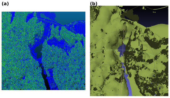
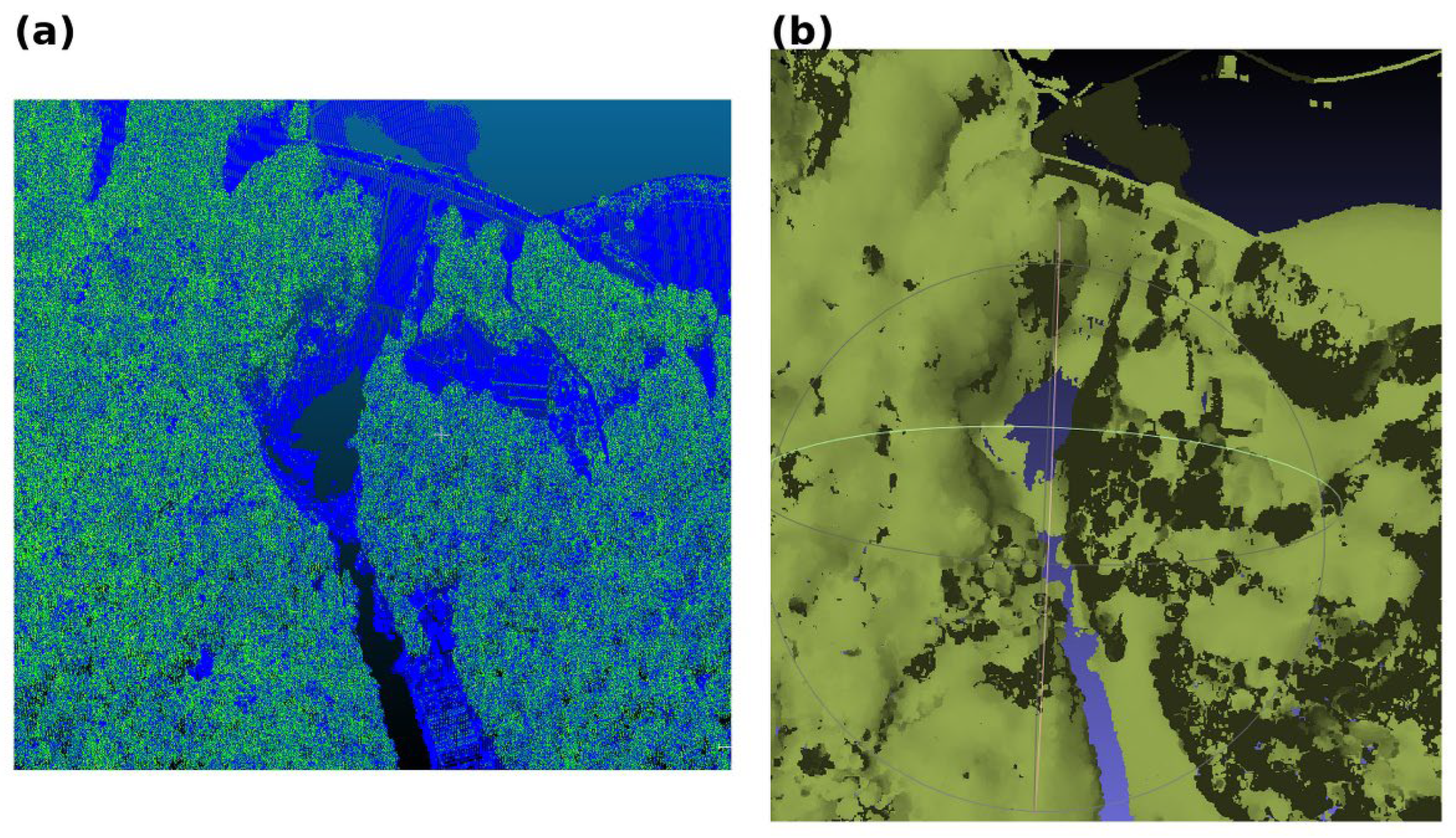
The LiDAR data obtained for Cleveland Dam and Capilano River in North Vancouver was originally provided in LASer (LAS) file format with a resolution of 1 m and 46,569,718 points, as shown in Figure 1a. The LAS format [55] is used to exchange and store LiDAR point cloud information. The LAS file was converted to STL format, which is compatible with DualSPHysics code.

For this purpose, the LAS file was first converted to the Polygon (PLY) file format as an intermediary step, due to the absence of a direct converter from LAS to STL; the resulting point cloud in PLY format is shown in Figure 1b. Subsequently, the PLY file was converted to STL format using the Ball Pivoting Algorithm (BPA)—a method used to generate a triangle mesh from a given point cloud. At its core, BPA determines triangles using a ball with a specified radius that touches three points without enclosing others [56]. By specifying a one-meter ball radius, the BPA preserved a consistent 1 m resolution in the conversion process. The LiDAR-derived computational domain used in this study is provided in the Supplementary Materials.

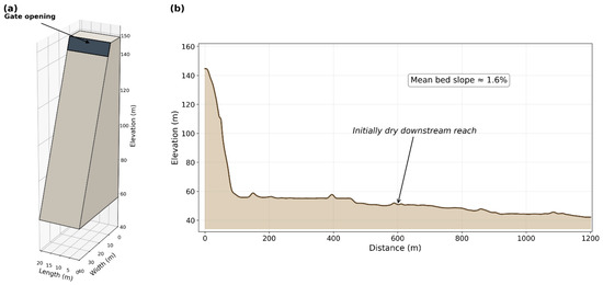
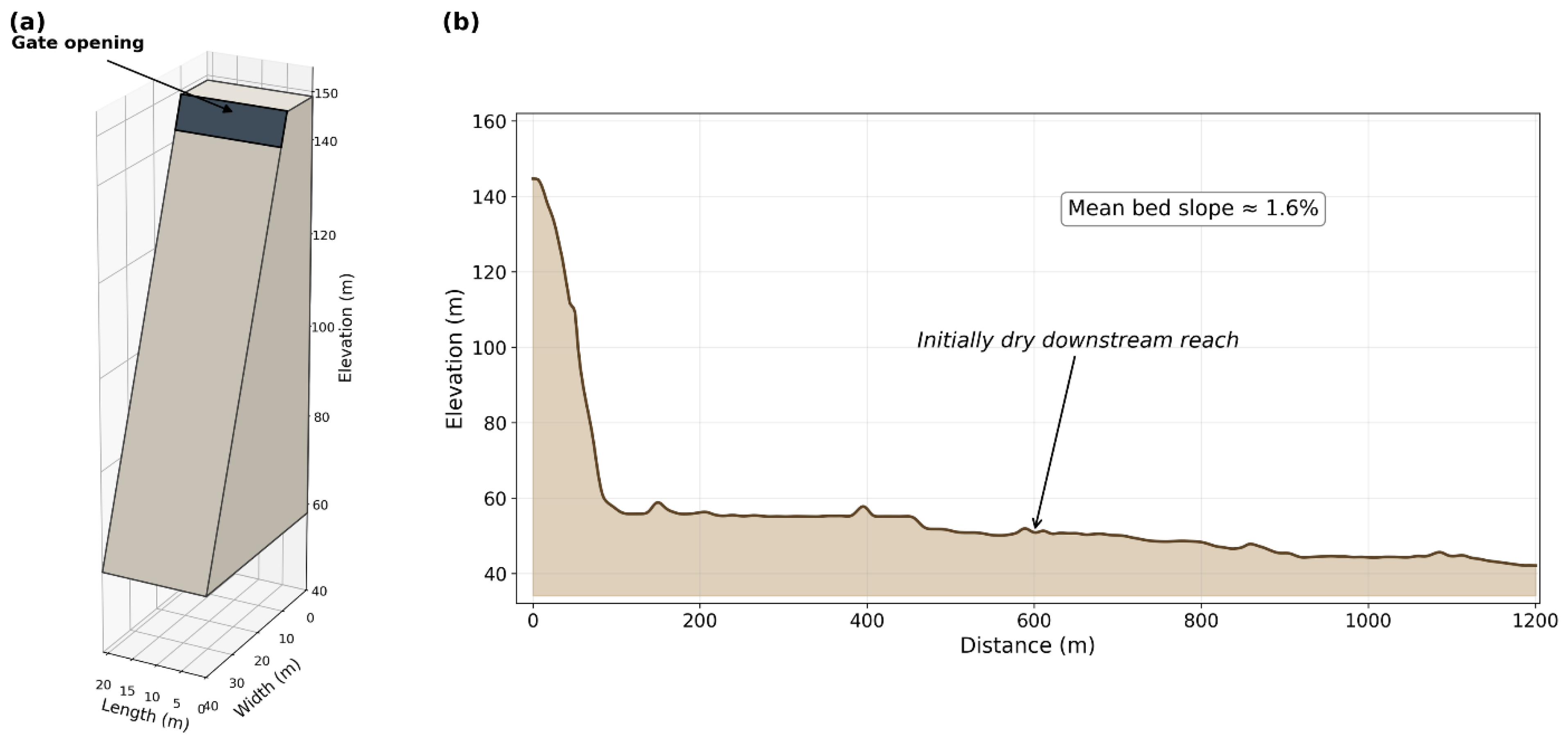
The geometry and dimensions of the dam, together with the position of the gate opening through which the release occurs, are shown in Figure 2a. The dam is 91 m high, while the gate opening—which controls discharge from the reservoir—measures 21 m by 7 m. Figure 2b presents the bed elevations along the river centerline, from the reservoir upstream to the downstream limit of the computational domain; the downstream reach is initially dry, corresponding to a zero water level, such that the flood wave released from the reservoir propagates over an initially dry bed.

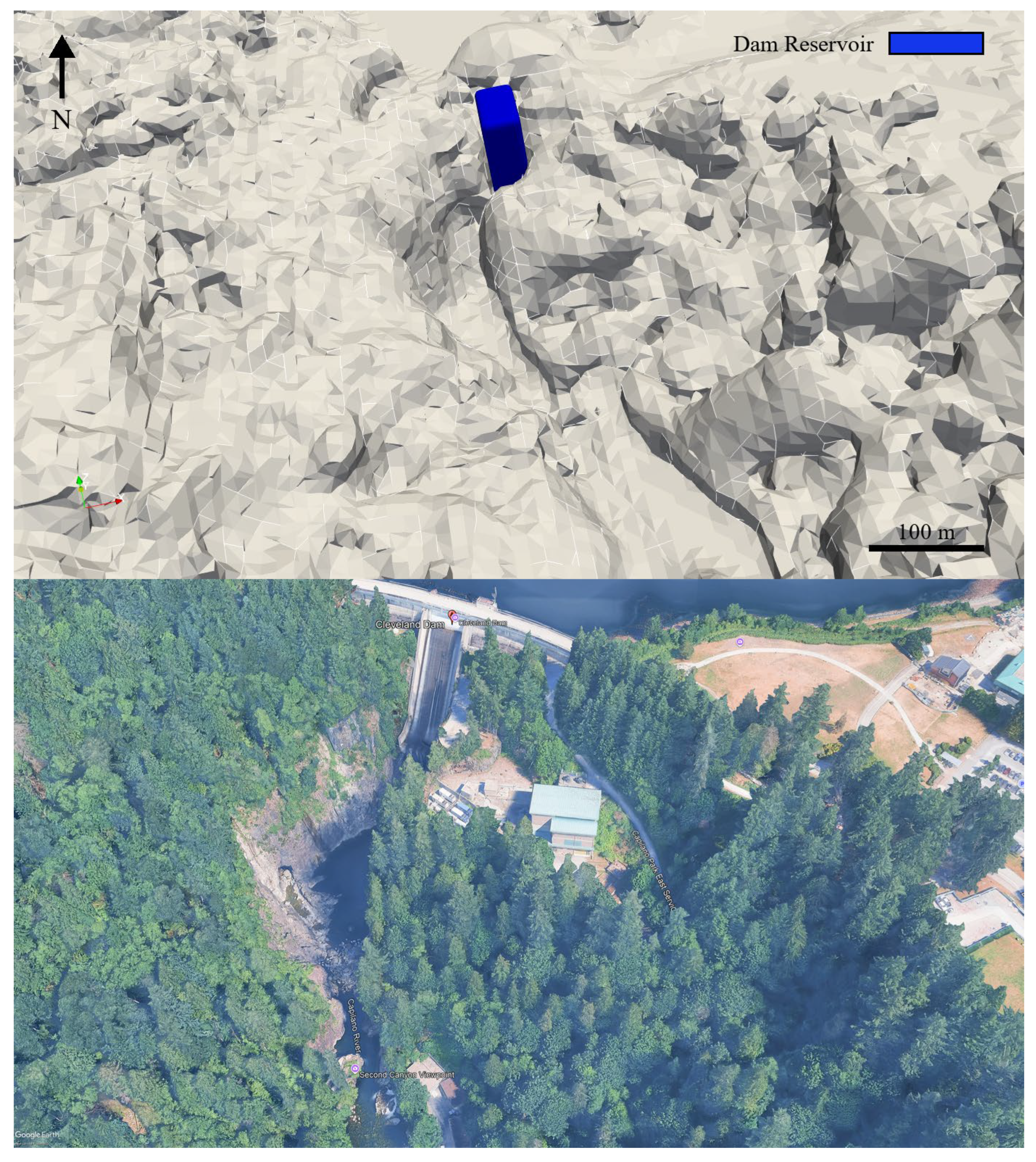
Figure 3 shows the computational domain of the chosen area surrounding the dam. The blue area represents the portion of the reservoir included in the SPH model, maintaining flow in the river for approximately 50 s, exceeding the 30 s period analyzed in this study. The figure also includes a real-world image of the same area obtained from Google Earth Pro [57], providing a visual comparison with the actual topography. The computational domain encompasses an area of 1200 m by 700 m.

The interparticle distance is analogous to the grid size in Eulerian models, with the initial particle interspacing r determining the Number of Particles (NoP) and particle arrangement within the computational domain at t = 0. For the reference simulation, the Wendland kernel was employed as the smoothing kernel. The r value was set to 2 m, resulting in a total NoP of 298,188 in the simulation. To mitigate numerical instabilities and prevent particle interpenetration, artificial viscosity was applied with a value of 0.25. Additionally, the mDBC was implemented to handle boundary interactions.

Temporal integration of the simulation was carried out using a Symplectic time-stepping algorithm with a CFL number of 0.2. Automatic smoothing length adjustment was implemented, where the smoothing length was adjusted based on the particle spacing and the local density of neighboring particles. This approach allows the smoothing length to be dynamically adapted with respect to changes in particle distribution and density, eliminating the need for manually predefined values [58]. The fluid properties were also defined with a density of 1000 kg/m³. The baseline configuration setup used for the simulations is provided in the Supplementary Materials.

The simulations were conducted using a workstation equipped with an NVIDIA RTX A2000 GPU with 12 GB of VRAM, supported by an Intel Core i9-13900H CPU and 32 GB of RAM. The GPU’s computational capabilities enabled efficient execution of the SPH simulations, while the CPU and RAM provided adequate resources for data management and pre/post-processing tasks. The total runtime of the simulation was 12 min.

3. Effects of SPH Numerical Parameters on WSE

This section evaluates how the selected SPH numerical parameters affect WSE predictions for the Cleveland Dam case. First, the WSE response under different numerical setups was compared through a parametric study, and recommends suitable ranges for the subsequent analysis. The individual and interaction effects of these parameters were then quantified, and the selected numerical setup was applied for a 3D dam-break simulation over the LiDAR-derived domain.

3.1. Parametric Study

First, the effects of the interparticle distance, smoothing length, time stepping schemes, artificial viscosity coefficient, and kernel function on the percentage difference in the average WSE and the highest WSE between selected models were assessed.

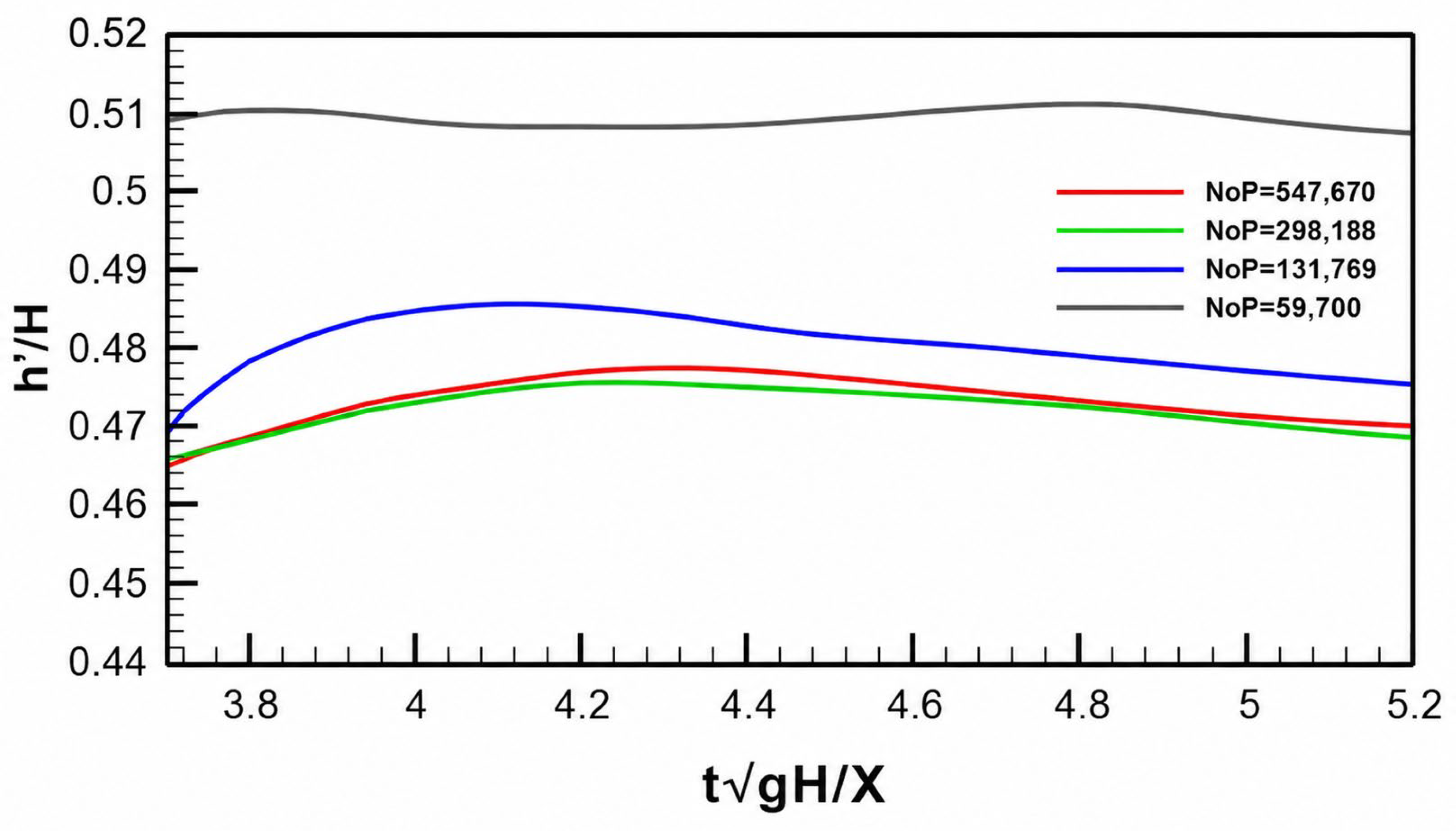
Four values of resolution or NoP are considered: 1.5 m (NoP = 547,670), 2 m (NoP = 298,188), 3 m (NoP = 131,769), and 4.5 m (NoP = 59,700). Finer resolutions result in higher particle counts and longer runtimes; specifically, simulations with r = 1.5 m required 25 min, while those with r = 2 m, r = 3 m, and r = 4.5 m took 12, 5, and 4 min, respectively.

The WSE, denoted as h’, was evaluated at a fixed point located 80 m downstream from the dam (X = 80 m), at the centerline of the channel, across various time steps. Figure 4 compares the dimensionless WSE expressed as h′/H, where H is the dam’s initial WSE, and dimensionless time for the four models. As the NoP increases, the wave profiles converge toward a unique wave profile across simulations; for example, the percentage difference in the average WSE between the models with r = 1.5 m and r = 2 m was only 0.048%, while the percentage difference in the highest WSE was 0.177%.

Based on Figure 4, r = 2 m (NoP = 298,188) was identified as the optimal resolution; in particular, the model with this resolution provides near-identical wave profiles to those obtained with the finest resolution (r = 1.5 m) while requiring less than half the runtime. Conversely, models with larger r values (r = 3 m and r = 4.5 m) showed deviations in WSE, demonstrating the trade-off between computational efficiency and result precision. Increasing the NoP beyond 298,188 particles offers limited improvements, making this setup recommended for further parametric studies.

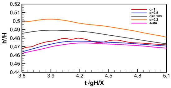
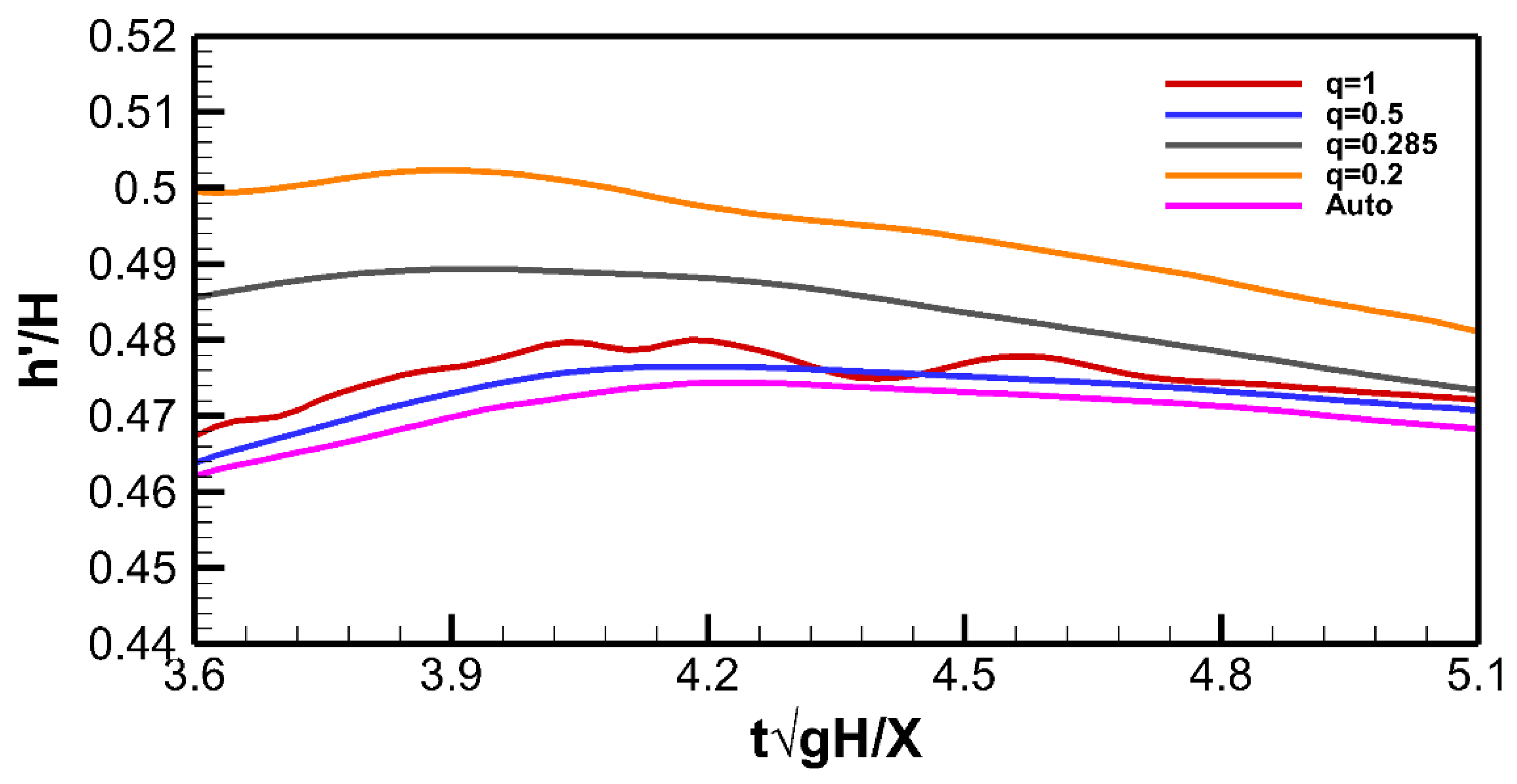
The effect of the smoothing length (h) was examined through the dimensionless ratio q = r/h, which controls the relative size of the support domain and defines the interaction region in the numerical approximation. According to Equations (6) and (7), q can theoretically range between 0 and 2. However, the choice of q must ensure sufficient particle interactions while avoiding excessive smoothing. In this study, six different q values were analyzed: q = 2, q = 1, q = 0.5, q = 0.285, q = 0.2, and q = 0.1.

Table 1. Smoothing lengths (h) and corresponding q values.

Smoothing Length	q = r/h
1	2
2	1
4	0.500
7	0.285
10	0.200
20	0.100

summarizes the smoothing lengths corresponding to these q values, with r = 2 m used in all simulations. Figure 5 shows the relationship between the dimensionless WSE and dimensionless time for different smoothing lengths and q values.

The computational runtime for all smoothing lengths was nearly identical, making accuracy the primary criterion for selecting h. When q = 2 (h = 1) or q = 0.1 (h = 20), no flow movement is observed after the dam breaks. These extreme values of q are unsuitable for the simulation, as they fail to capture the dynamics of the flow. Specifically, when q = 2, the support domain is too small, resulting in insufficient particle interactions; in contrast, for q = 0.1, the support domain is excessively large, leading to over-smoothing and the loss of local details.

Overall, the best range for the q value was found to be between 0.5 and 1; in particular, the percentage difference in the average WSE between the models with q = 0.5 and q = 1 was 0.46%, while the percentage difference in the highest WSE was 0.35%. Thus, both setups produce nearly identical results, making them suitable for future simulations. Conversely, q values outside this range (e.g., q = 0.285 or q = 0.2) resulted in noticeable deviations in the wave profile.

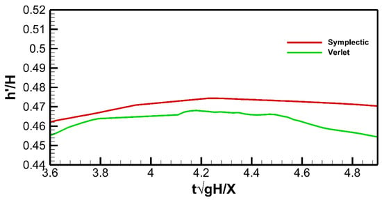
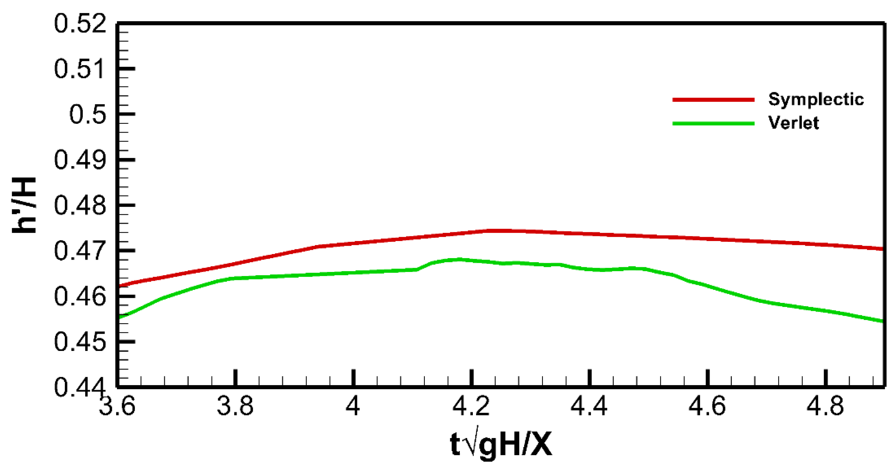
The effects of two time-stepping schemes—Symplectic and Verlet—were also evaluated. Figure 6 compares the two schemes by plotting the dimensionless WSE against dimensionless time. The percentage differences in the average and highest WSEs quantify the influence of a given scheme on the simulation results.

The differences in the wave profiles produced by the two schemes were greater than those observed for other parameters: the percentage difference in the average WSE between the two schemes was 0.87%, while the percentage difference in the highest WSE was 0.63%. The computational runtime differed slightly between the two schemes, with the Verlet-based scheme requiring 9 min and the Symplectic scheme requiring 12 min to complete the simulation. Both simulations were conducted on the workstation described in Section 2.3, and GPU-based parallel execution in DualSPHysics was used in both cases. Although the Verlet-based scheme reduced the runtime by approximately 25% in this case, this gain remains moderate relative to the total simulation time. Given this moderate gain, the Symplectic scheme was adopted for the subsequent simulations. The Verlet-based scheme would have been used if the runtime reduction exceeded 50% while the WSE differences remained limited.

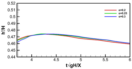
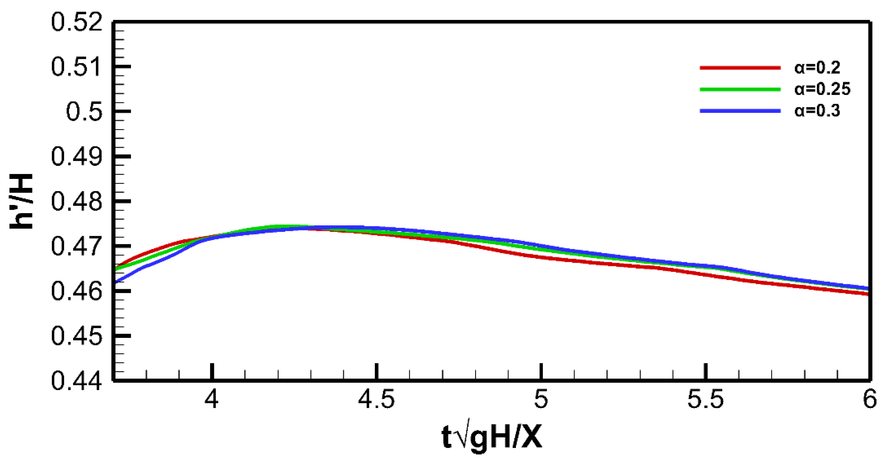
In this study, the effects of three different artificial viscosity coefficient values (0.2, 0.25, and 0.3) were analyzed. Figure 7 presents the dimensionless WSE as a function of dimensionless time. All three values produced similar wave profiles; for example, the percentage difference in the average WSE between α = 0.2 and α = 0.3 was 0.046%, while the percentage difference in the highest WSE was 0.022%. These small differences suggest that the range from α = 0.2 to α = 0.3 is recommended for achieving accurate results.

Additional simulations conducted for α values outside this range led to results that were significantly different from those obtained with α = 0.2 to α = 0.3; for example, at α = 0.1, the wave profile exhibited unphysical oscillations, while at α = 0.4, excessive damping was observed, resulting in a flattened wave profile. These deviations indicate that α values outside the range of 0.2 to 0.3 fail to accurately capture the dynamics of the dam-break flow.

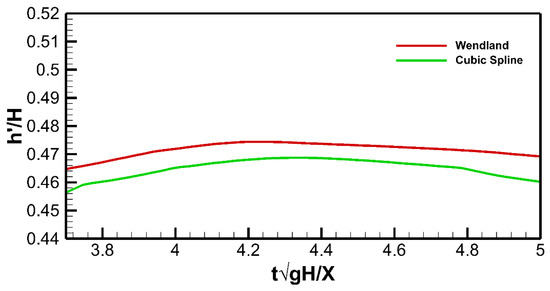
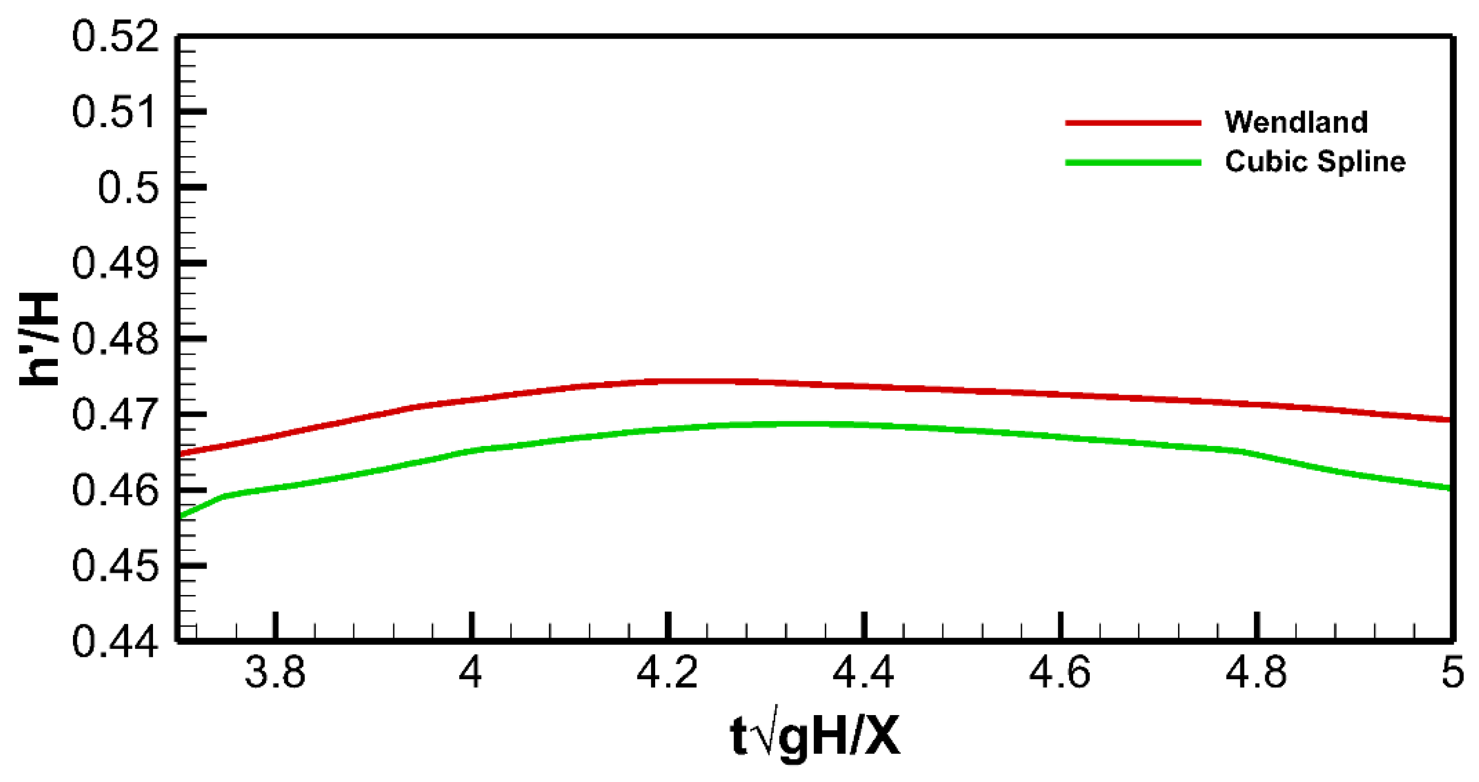
The cubic spline kernel and the Wendland kernel were examined to assess their influence on the dam-break flow simulation. Figure 8 compares the dimensionless WSE against dimensionless time for these two kernel functions. As for the other parameters, the kernel function’s influence on the simulation results was quantified by calculating the percentage differences between the average and highest WSE.

Both kernel functions produced similar wave profiles, with only minor differences observed; specifically, the percentage difference in the average WSE between the two kernel functions was 0.2%, while the percentage difference in the highest WSE was 0.56%. Thus, both the cubic spline and Wendland kernels are effective in capturing the dynamics of the dam-break flow. Furthermore, the computational runtime for both kernel functions was nearly identical. Based on these results, both the cubic spline and Wendland kernels are recommended for SPH simulations of dam-break flows. The recommended numerical parameter values and ranges obtained from the parametric study are summarized in

Table 2. Recommended SPH numerical parameter values and ranges for dam-break simulations.

Parameter	Recommended Value or Range	Justification
Interparticle distance	r = 2 m	Near-identical WSE profiles are obtained compared with r = 1.5 m, with less than half the runtime.
Smoothing-length ratio	0.5 ≤ q ≤ 1	Similar WSE profiles are obtained within this range, while values outside the range produce noticeable deviations or loss of flow resolution.
Time-stepping scheme	Symplectic	Improved time-integration accuracy is provided, while the runtime reduction obtained with the Verlet-based scheme remains moderate.
Artificial viscosity coefficient	0.2 ≤ α ≤ 0.3	Similar WSE profiles are obtained within this range, while lower or higher values produce oscillations or excessive damping.
Kernel function	Cubic spline or Wendland	Comparable WSE responses and nearly identical computational runtimes are obtained with both kernels.

.

3.2. Sensitivity Analysis of Numerical Parameters

To extend the parametric study beyond single-parameter comparisons, a sensitivity analysis was conducted to quantify the effects of three numerical parameters on the predicted maximum WSE. This analysis allows for quantitative assessment of the relative importance of parameters and their interaction effects. A surrogate-based framework enabled the computation of sensitivity indices.

The polynomial order and the regression strategy for the Polynomial Chaos Expansion (PCE) surrogate model were selected based on the leave-one-out (LOO) cross-validation error. Among the tested combinations, a second-order PCE with the Least Angle Regression (LARS) approach yielded the minimum LOO error. The resulting PCE surrogate was subsequently employed to compute first- and second-order Sobol’ sensitivity indices. In this analysis, NoP and the time-stepping scheme were fixed based on the preceding parametric assessment. In particular, NoP was fixed at 298,188 particles because this resolution produced near-identical WSE profiles to those obtained with 547,670 particles while requiring less than half the runtime, and further refinement provided only limited improvement. Furthermore, the Symplectic scheme was selected because its half-step updates and intermediate force evaluations provide tighter temporal coupling and improved accuracy in time integration, whereas the Verlet-based scheme was found to reduce the runtime by only approximately 25%. Therefore, the sensitivity analysis focused on the smoothing length, kernel function, and artificial viscosity coefficient.

The sensitivity analysis used the same parameter ranges as the parametric study, with 50 samples generated for each case, and WSE used as the model output. This analysis was conducted for representative dam heights of 80 m, 90 m, and 100 m.

Table 3. First-order Sobol’ indices for H = 80, 90, and 100 m.

Parameter	Sobol’ Index (H = 80 m)	Sobol’ Index (H = 90 m)	Sobol’ Index (H = 100 m)
h	0.681	0.676	0.700
Kernel	0.149	0.180	0.171
α	0.045	0.035	0.039

reports the first-order Sobol’ indices for the selected numerical parameters, quantifying their individual contributions to the variance of the predicted WSE for the three cases. The results indicate that the smoothing length is the dominant parameter, while the kernel function exhibits a moderate influence. In contrast, the artificial viscosity coefficient contributes only marginally within the investigated range.

Table 4. Second-order Sobol’ indices for H = 80, 90, and 100 m.

Parameter Interaction	Sobol’ Index (H = 80 m)	Sobol’ Index (H = 90 m)	Sobol’ Index (H = 100 m)
h–Kernel	0.123	0.102	0.088
α–Kernel	0.000	0.005	0.000
α–h	0.000	0.000	0.000

presents the second-order Sobol’ indices. The interaction between the smoothing length and the kernel function represents the most significant interdependence in all cases. The remaining interactions are negligible, indicating limited coupled effects between the artificial viscosity coefficient and the other parameters.

3.3. Numerical Simulation

Next, the numerical parameters recommended in Section 3.1 were applied to study the three-dimensional dam-break flow at the Cleveland Dam. The results are presented for the temporal evolution of the dam-break flow, the spatial distribution of WSE, and water surface profiles at different cross-sections.

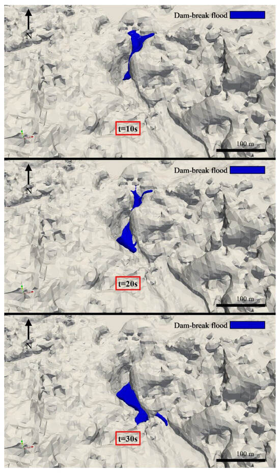
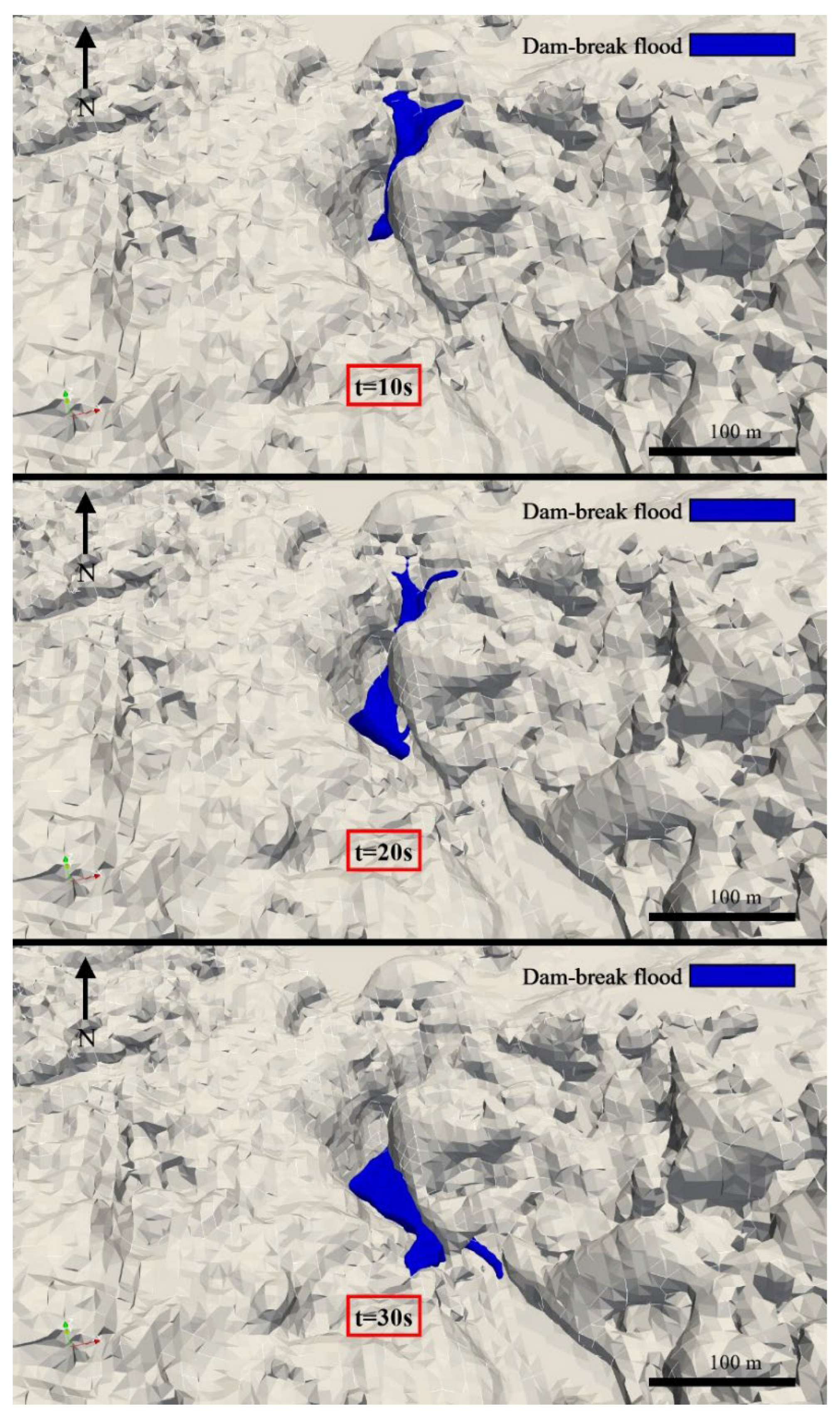
The results of the 3D dam-break simulation are presented in Figure 9, illustrating the flow evolution at three distinct dimensionless time instances, t = 0.17, t = 0.33, and t = 0.50, corresponding to t = 10 s, t = 20 s, and t = 30 s, respectively. The total released flood volume during the dam-break event was approximately 12,500 m³. The water column collapses due to gravitational forces, propagating along the dry horizontal bed; as the flow progresses downstream, the Capilano River’s curved terrain influences the flood behavior.

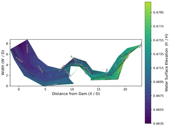
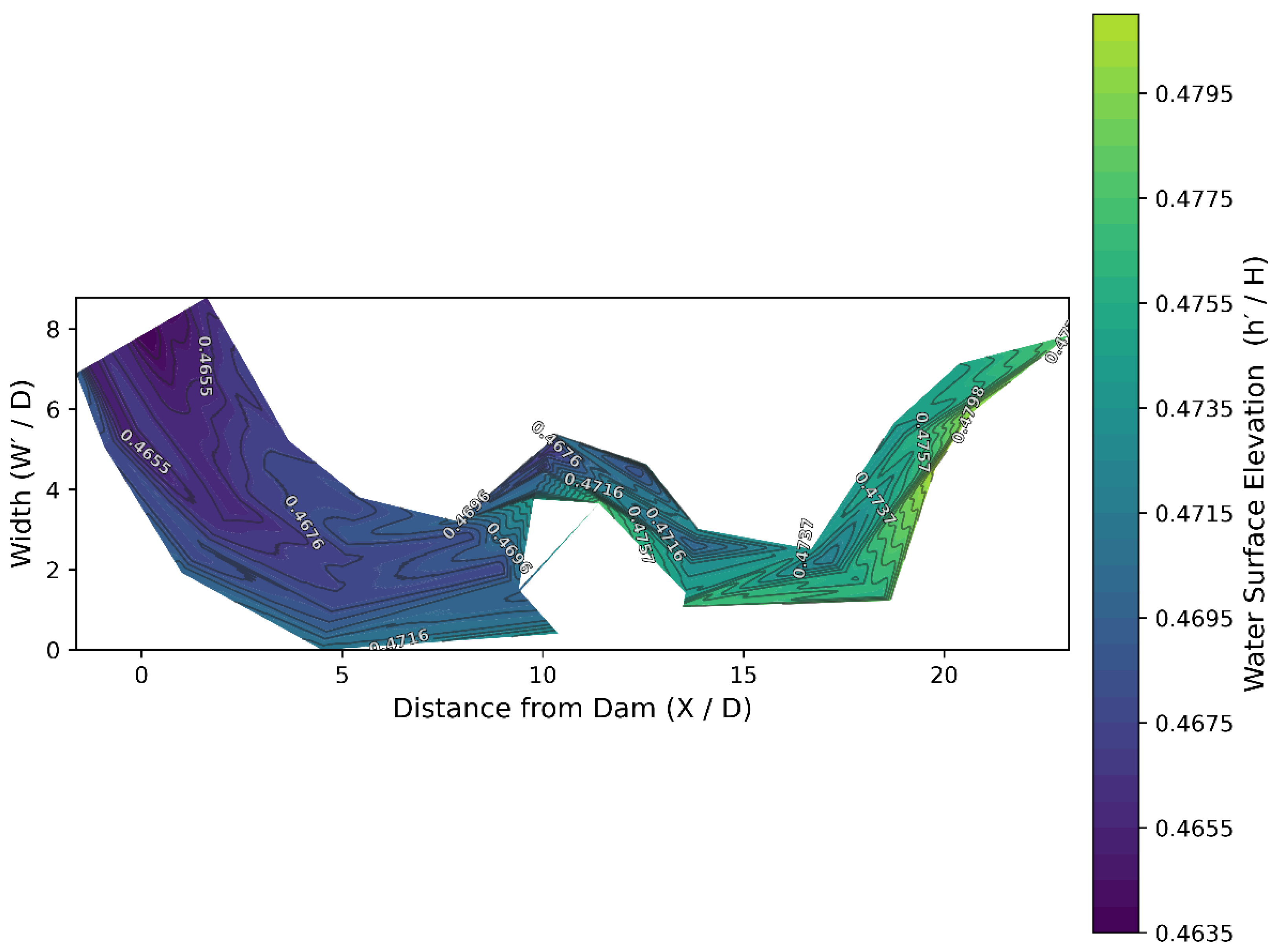
Figure 10 illustrates the isosurface map of the WSE at t = 0.5. The horizontal axis represents the dimensionless length of the river (defined as X/D, where X is the distance from the dam and D is the hydraulic depth, defined as cross-sectional flow area divided by water surface width evaluated at the reference Section 80 m downstream of the dam). The dam is located at X/D = 0 on the left side of the figure, and the flow direction is from left to right, with the downstream end at X/D = 21.92. The vertical axis indicates the dimensionless width of the cross-section (defined as $W^{\prime }/D$, where $W^{\prime }$ is the width at each specific location). The WSE after the dam-break, h′/H, is normalized by the initial WSE.

The map was constructed from 12 cross-sections spanning from 6.85 to 21.92 at a uniform spacing of 1.37, with values between sections linearly interpolated along the flow direction. The contour patterns highlight variations in WSE, especially near the upper and lower edges of the figure (representing the left and right riverbanks, respectively), and toward the right side of the plot (corresponding to the downstream region). At X/D = 21.92, the water surface flattens. The rapid elevation fluctuations diminish, suggesting a more uniform WSE as the flood wave advances.

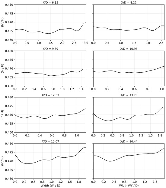
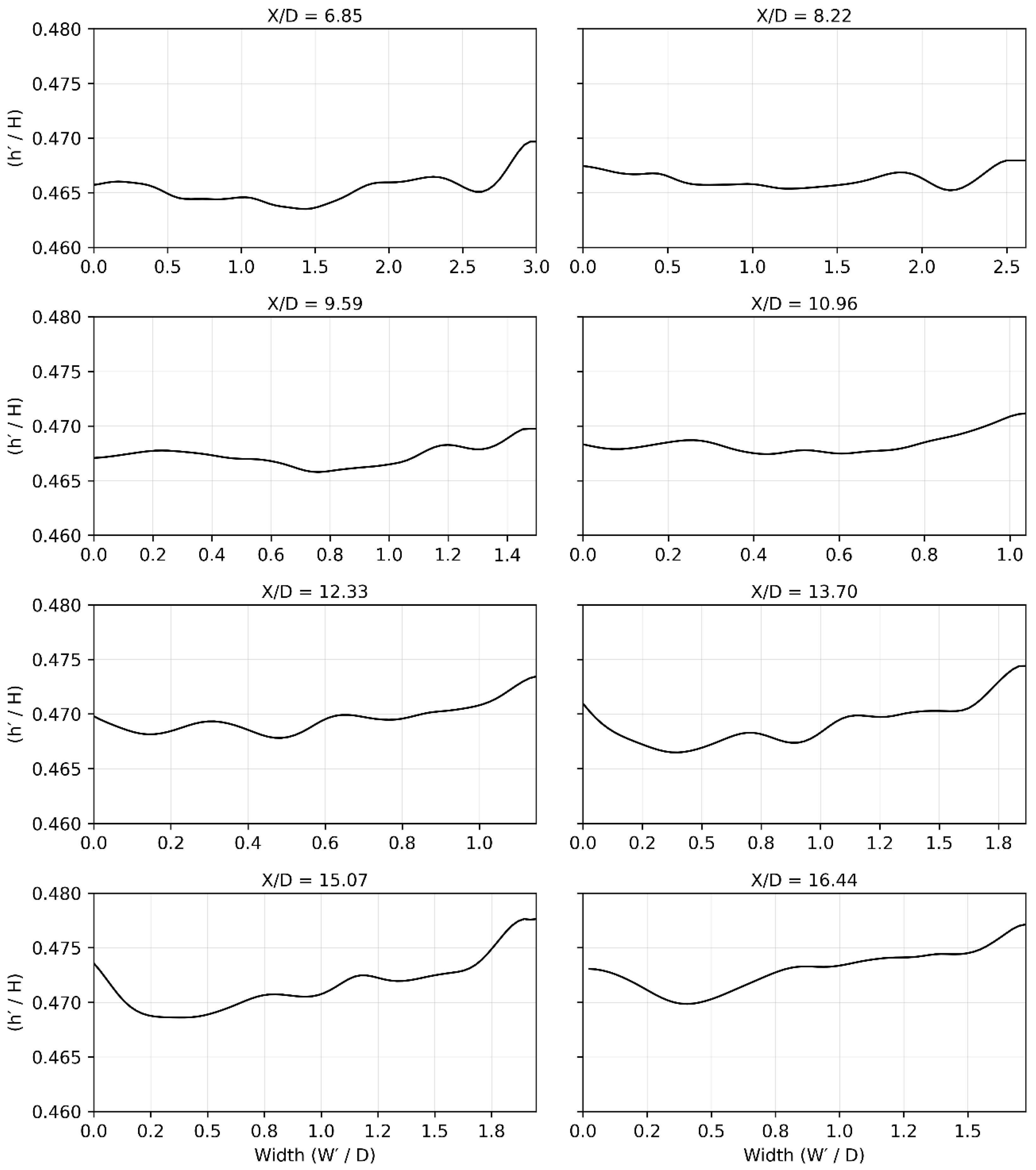
Figure 11 depicts the water surface profiles across 8 distinct cross-sections of the river at t = 0.5. The vertical axis corresponds to the dimensionless WSE (h′/H), while the horizontal axis indicates the dimensionless width of the cross-section ($W^{\prime }/D$), as described for Figure 10. The maximum value of the horizontal axis varies among the plots because each cross-section has a different river width. Each cross-section is annotated with a corresponding X value; for example, an annotation of X/D = 16.44 indicates that the respective cross-section is located 60 m downstream from the dam. The WSE evolution profiles at different cross-sections along the river at t = 0.5 reveal the spatial distribution of water levels across the width of the river. The variations in h′/H across the sections represent the large free-surface deformation of the dam-break flow over the irregular riverbed. In these profiles, the left side of each plot (W′/D = 0) corresponds to the right bank of the river, and the right side corresponds to the left bank. It was assumed that the initial condition represents a dry bed, meaning the WSE before flooding is 0.

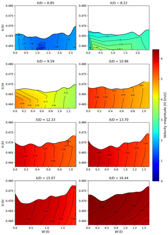
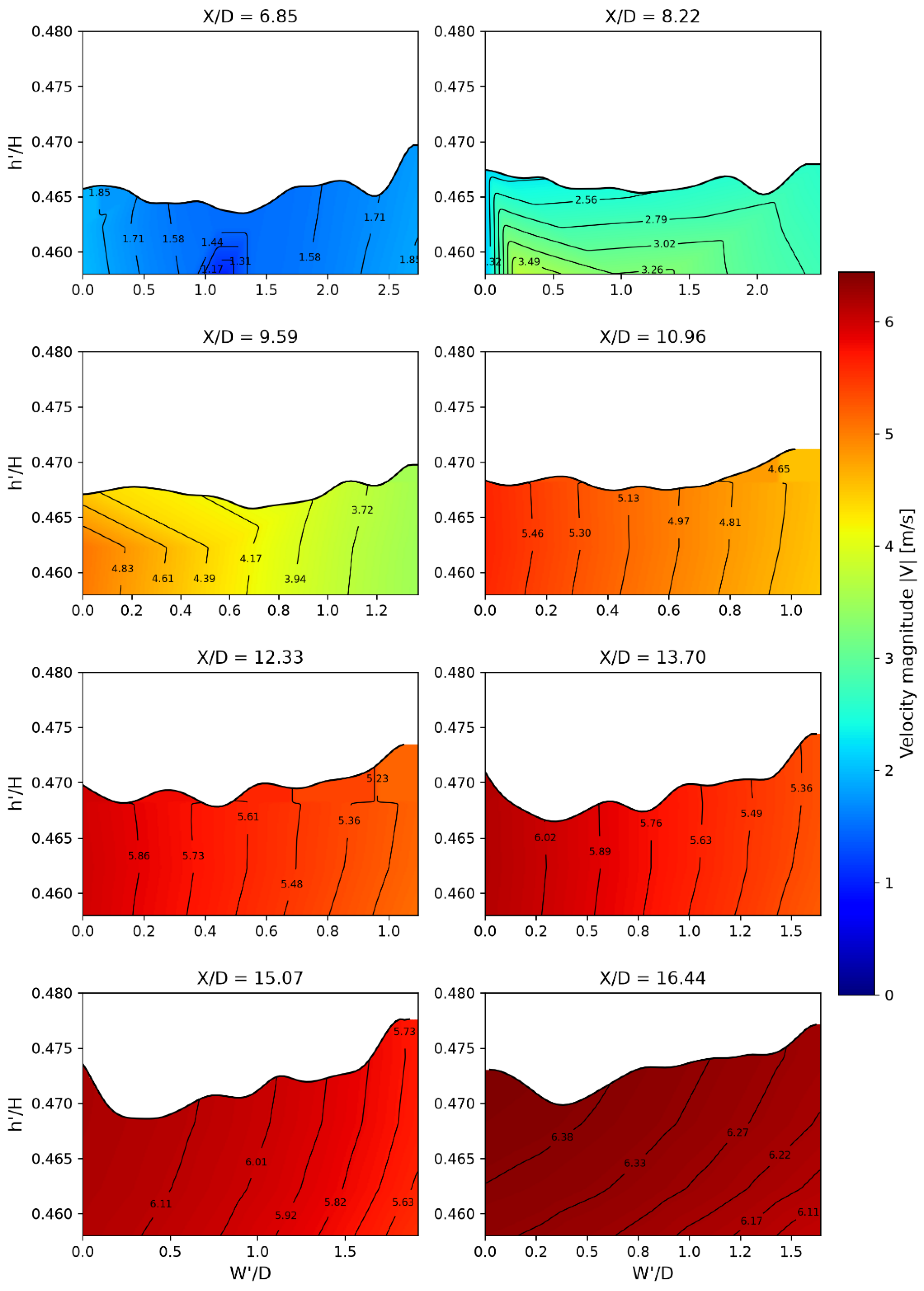
Figure 12 presents the velocity field distribution contours across 8 distinct cross-sections of the river at t = 0.5. The vertical axis corresponds to the dimensionless WSE (h′/H) and the horizontal axis indicates the dimensionless width of the cross-section (W′/D), as described above, with each cross-section annotated by its corresponding X/D value. Within each cross-section, the velocity magnitude was found to be largest near W′/D = 0 (i.e., along the right bank of the river) and decreases toward the left bank, reflecting the influence of the curved terrain of the Capilano River on the flow distribution across its width.

Table 5. Summary of the velocity magnitudes at the 8 cross-sections of the river at t = 0.5.

X/D	X (m)	V_Min (m/s)	V_Mean (m/s)	V_Max (m/s)
6.85	25	0.852	1.63	2.00
8.22	30	2.02	2.94	4.02
9.59	35	3.50	4.15	5.06
10.96	40	4.47	5.05	5.62
12.33	45	5.09	5.57	5.99
13.70	50	5.21	5.70	6.15
15.07	55	5.50	5.95	6.20
16.44	60	6.02	6.29	6.44

summarizes the minimum, mean, and maximum velocity magnitudes at the 8 cross-sections at t = 0.5. The mean velocity magnitude increased steadily in the downstream direction, from X/D = 6.85 to X/D = 16.44. This trend occurs because, at t = 0.5, the flood wave front had advanced into the downstream reach, while the flow in the upstream sections had already decelerated as the reservoir emptied.

The spatial patterns observed in Figure 9, Figure 10, Figure 11 and Figure 12 highlight the three-dimensional nature of dam-break flood propagation. The results indicate a non-uniform distribution of WSE across successive cross-sections, with more pronounced variations near the riverbanks. These patterns reflect the combined influence of complex topography and flow expansion on the evolving flood wave.

4. Verification of the Parameter Ranges

4.1. Verification Against a Two-Dimensional Shallow Water Model

To further assess the quality of the numerical results obtained from the three-dimensional SPH simulations, a comparative analysis was carried out with the same test case using a two-dimensional HEC-RAS model based on the SWEs [11]. This model was solved under unsteady flow conditions, with flow resistance represented by Manning’s roughness coefficient. This comparison allowed for examination of the consistency of the predicted WSEs obtained from the SPH framework with those produced with a widely used depth-averaged approach.

The HEC-RAS computational domain was defined using the same LiDAR-derived topography used in the SPH model. The roughness coefficient was calibrated specifically for the main channel using observed water depth data from the Cable Pool gauge station located in the Capilano River. Manning’s roughness coefficients range from 0.020 to 0.060 and were tested iteratively, consistent with previous HEC-RAS roughness calibration studies [59,60]. For each tested value, the simulated water depth response was compared with the observed data, and the coefficient providing the closest agreement was selected. This calibration was performed under transient conditions to account for the rapid variations in flow depth and velocity associated with the dam-break process [61,62]. Following this procedure, a final Manning’s roughness coefficient of n = 0.037 was obtained and used for the subsequent comparison.

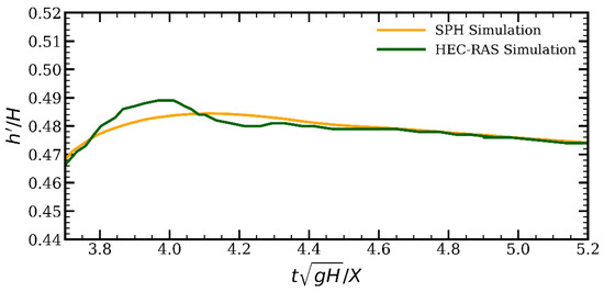
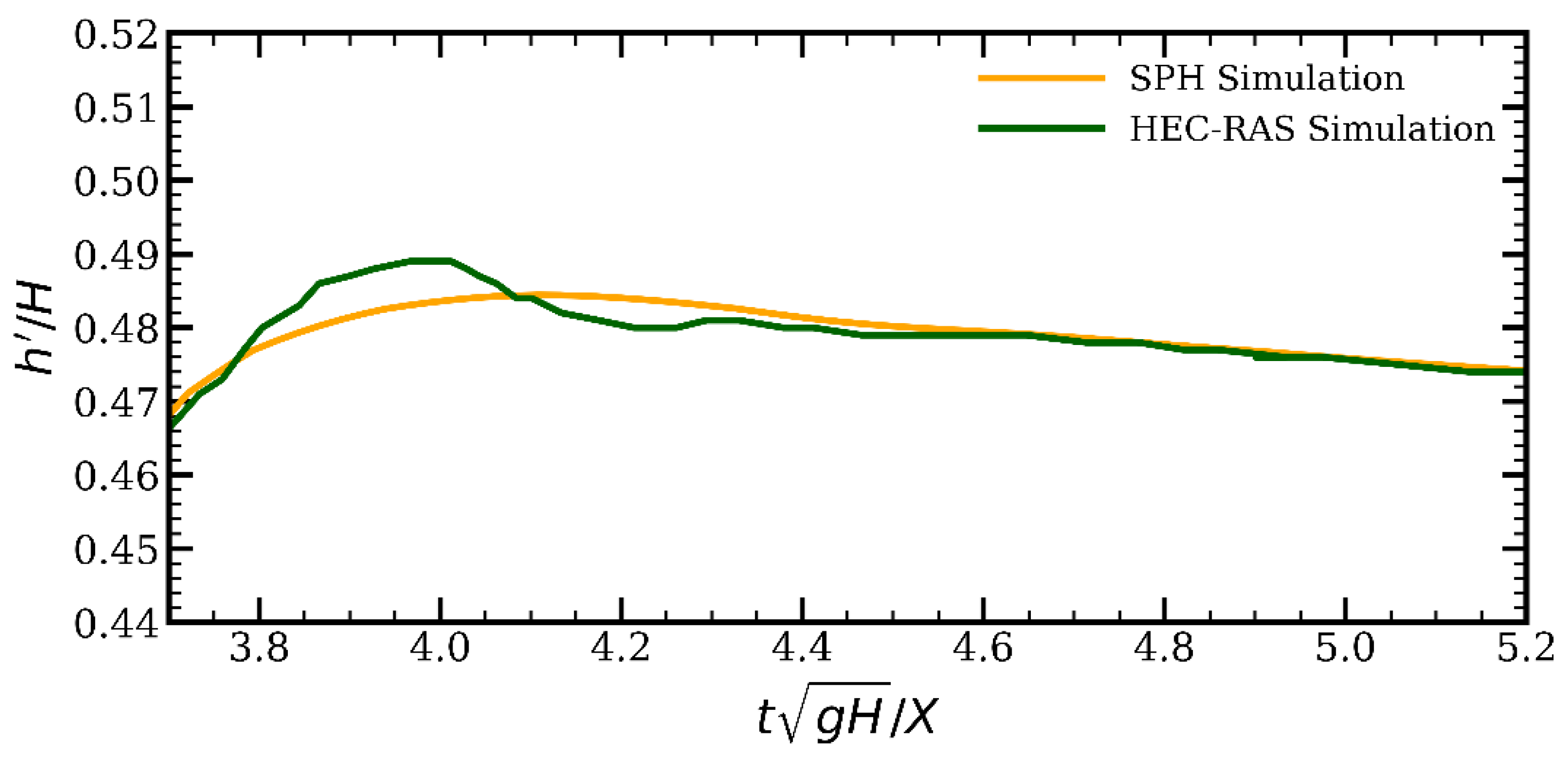
After calibration, the WSE predicted using the HEC-RAS model was extracted at 80 m downstream from the dam and compared with the corresponding results obtained from the SPH simulations. The agreement between the two models was evaluated using the Ratio of the Root Mean Square Error to the Standard Deviation (RSR).

Figure 13 presents the comparison between the WSE predicted using the SPH model and the corresponding results obtained from the HEC-RAS simulation. The agreement between the two models is quantified using the RSR, with a value of 0.331, indicating a close correspondence between the predicted water surface profiles. According to the performance criteria proposed by Moriasi et al. [63,64], an RSR value lower than 0.5 denotes very good agreement, confirming that the SPH model accurately reproduces the WSE predicted by the depth-averaged reference model at 80 m downstream from the dam.

4.2. Verification Against a 2D Classical Dam-Break Test Case

A 2D dam-break test case was used to verify that the numerical parameter ranges and modeling choices identified in Section 3.1 lead to consistent results when applied to an independent dam-break benchmark. The 2D dam-break setup is widely used in the literature as a reference problem, due to its controlled conditions and the availability of experimental measurements [36,65,66].

The validation test case corresponded to a two-dimensional classical dam-break experiment conducted in the Civil Engineering Hydraulics Laboratory of Çukurova University, Turkey [67]. The experimental setup was arranged in a rectangular channel with internal dimensions of 8.90 m in length, 0.30 m in width, and 0.35 m in height. A vertical dam was positioned 4.65 m from the channel entrance, creating an upstream reservoir. The initial water depth in this reservoir was taken as 0.25 m, while the downstream region was kept dry.

For the numerical model, the Wendland kernel was implemented together with a Symplectic time-stepping scheme. The artificial viscosity coefficient, α, was set to 0.25, consistent with the range identified in the parametric analysis, where values between 0.2 and 0.3 were found to produce convergent wave profiles. The ratio between particle spacing and the smoothing length, q, was set to 0.5, following the findings in Section 3.1.

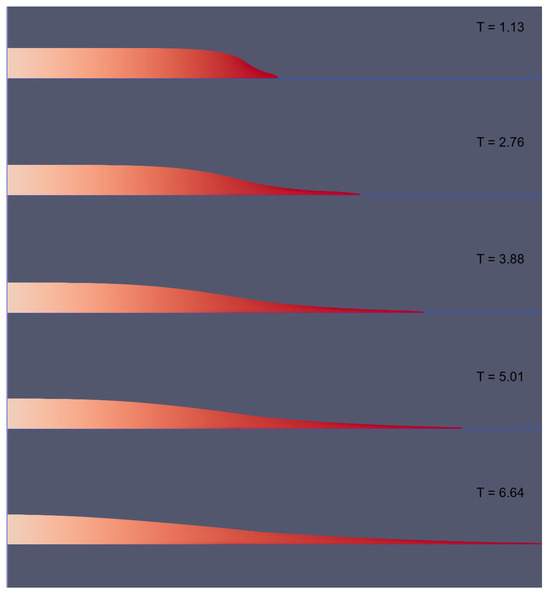
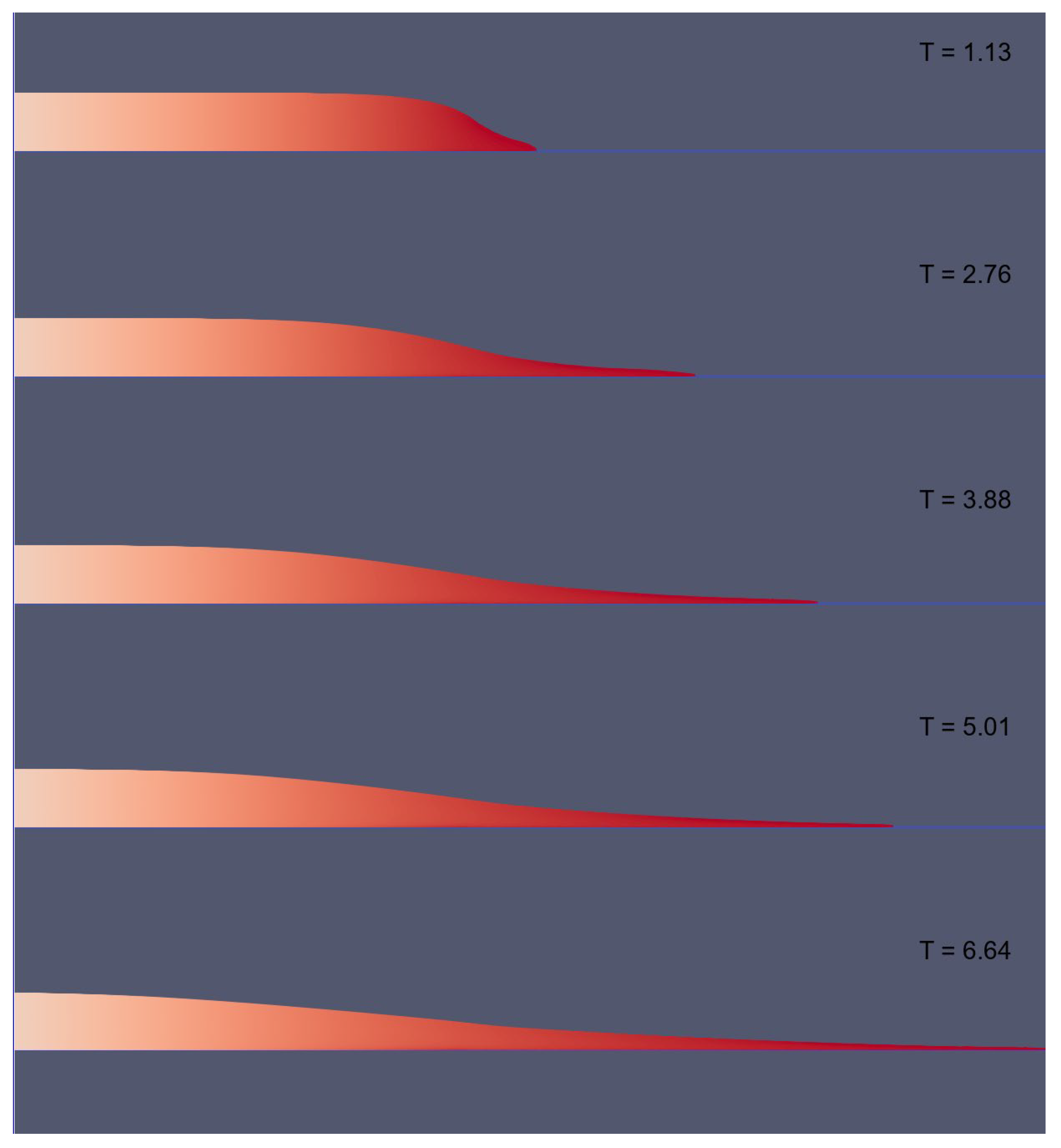
Figure 14 illustrates the free-surface evolution obtained from the SPH model at five distinct instants during the dam-break process. To enable a consistent comparison with the experimental data, the physical time, t, was normalized using the characteristic scaling ${(g/H_v)}^{0.5}$, where H_v is the initial water depth in the reservoir. The resulting dimensionless time is denoted by $T$, and the five snapshots shown in the figure correspond to T = 1.13, 2.76, 3.8, 5.01, and 6.64. These images are used to represent the temporal progression of the dam-break wave as it propagates along the channel.

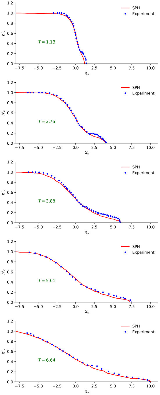
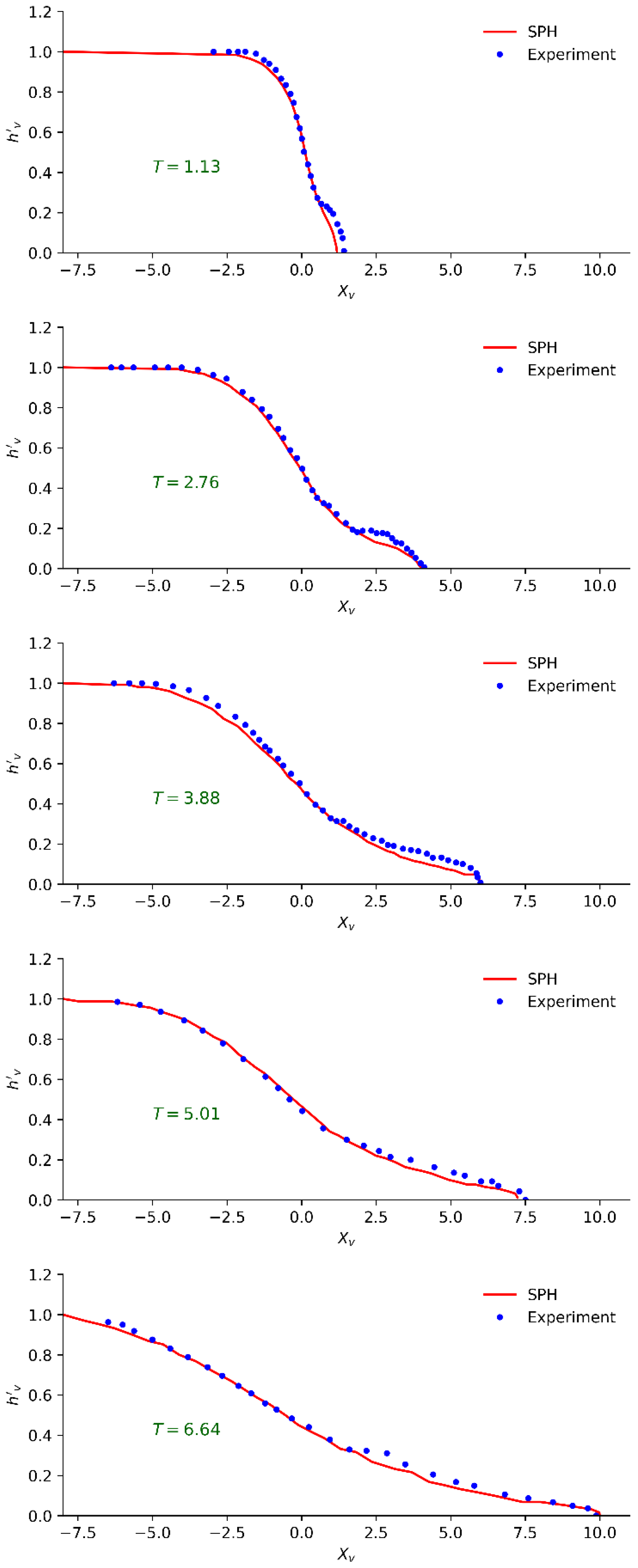
Figure 15 presents the comparison between the computed free-surface profiles obtained with the SPH model and the corresponding experimental measurements at the same dimensionless times T. Both the horizontal length and the flow depth were normalized by the initial water depth H_v, yielding the dimensionless variables X_v and h’_v, respectively. The numerical assessment of the model performance is provided in

Table 6. Dimensionless statistical measures evaluating the agreement between the SPH results and the experimental free-surface profiles for different T values.

T	R2	RMSE	MAE	MBE
1.13	0.983	0.039	0.030	0.028
2.76	0.994	0.024	0.020	0.020
3.88	0.990	0.033	0.029	0.029
5.01	0.995	0.021	0.016	0.008
6.64	0.993	0.023	0.018	0.017

, where the statistical measures are reported for each value of T. Since these measures were computed from the dimensionless depth h′v, the reported RMSE, MAE, and MBE values are dimensionless.

The discrepancies reported in Table 6 are consistent with the RMSE range of 0.01–0.10 reported by Magdalena and Pebriansyah [12] and the R² values of up to approximately 0.96 obtained by Ferdowsi et al. [13] for classical dam-break simulations, indicating an acceptable level of agreement.

4.3. Verification Against a 3D Dam-Break Test Case Through a 45° Bend Channel

To extend the previous 2D verification (Section 4.2) to a more complex setup, a 3D dam-break test case involving a bend channel—thus combining the effects of flow turning and three-dimensional propagation—was considered. Validation was conducted using a well-established dam-break benchmark developed within the CADAM (Concerted Action on Dam-Break Modeling) program, which provides experimental data for model verification [68]. This benchmark was derived from controlled dam-break experiments conducted in the Civil Engineering Department Laboratory of the Université catholique de Louvain, Belgium, in which a reservoir was connected to a straight channel followed by a 45° bend, and is included in the CADAM program for dam-break model verification [68,69]. The configuration was designed to reproduce the effect of an abrupt change in flow direction, a condition under which one-dimensional approaches may fail to predict the maximum water level and the wave arrival time [69]. The engineering relevance of this configuration is associated with flood propagation through curved natural rivers and engineered channels, where flow turning produces non-uniform water depth and velocity distributions across the section. A comparable effect is observed in the Cleveland Dam case, where the curved terrain of the Capilano River produces non-uniform WSE and velocity distributions across the river, while lower velocities are obtained in the upstream sections at t = 0.5 as the reservoir empties. The two configurations also share the same physical structure; namely, a reservoir released onto an initially dry downstream reach. The benchmark was therefore used to assess the recommended SPH setup under controlled three-dimensional flow-turning conditions, with gauge G4 (located within the bend) providing direct verification that the recommended parameter ranges reproduce the flow behavior in a curved reach.

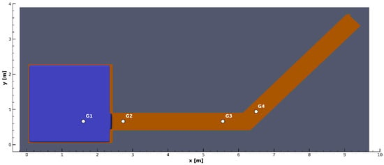
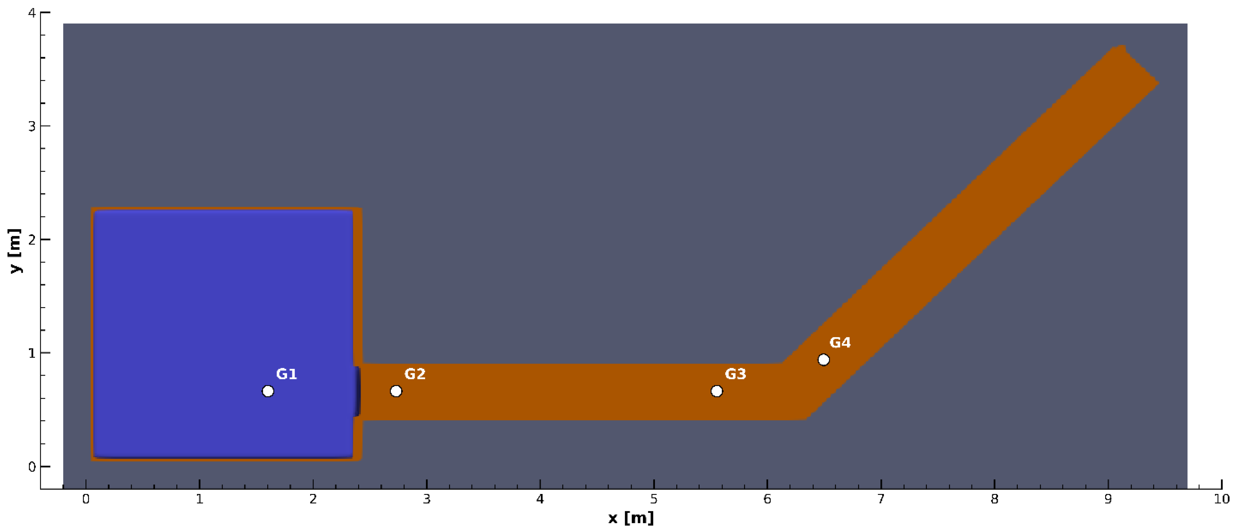
In addition to the numerical parameters obtained in the present study, an additional simulation was performed using basic values of numerical parameters that are physically consistent, in order to evaluate the influence of parameter selection. Furthermore, the water depths were compared to the SPH numerical results reported by Kao and Chang [16]. The computational domain and measurement locations are illustrated in Figure 16. The computational domain consisted of a square reservoir connected to a horizontal channel followed by a 45° bend, with the geometric dimensions defined in the figure. The initial water depth in the reservoir was 0.25 m, while the downstream channel was initially dry. Four gauges (G1–G4) were positioned along the flow path, with G1 located inside the reservoir, G2 and G3 along the straight channel, and G4 within the bend section, allowing for evaluation of flow propagation and water depth evolution throughout the domain. The recommended numerical setup comprised a Wendland kernel, a Symplectic time-stepping scheme, an artificial viscosity coefficient of 0.25, and a particle spacing to smoothing length ratio (q) of 0.5, with a total number of particles of approximately 300,000.

In contrast, the basic setup was defined by modifying four numerical parameters outside the ranges recommended in Section 3. Specifically, a Verlet time-stepping scheme was employed, the artificial viscosity coefficient was increased to α = 0.4, the particle spacing to smoothing length ratio was set to q = 0.285, and the total number of particles was reduced to approximately 200,000. Additionally, the results corresponding to the best-performing parameters in the research of Kao and Chang [16] were selected for comparison in the present study.

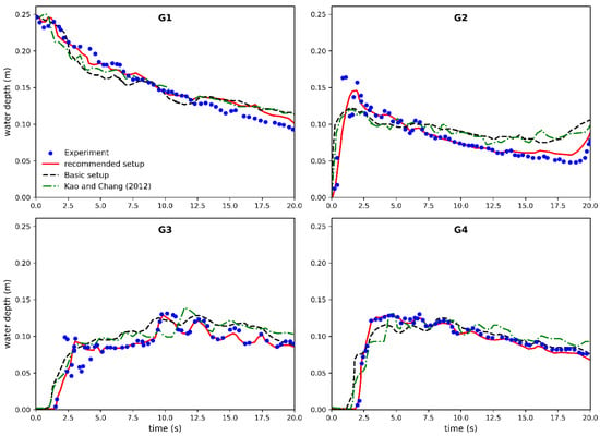
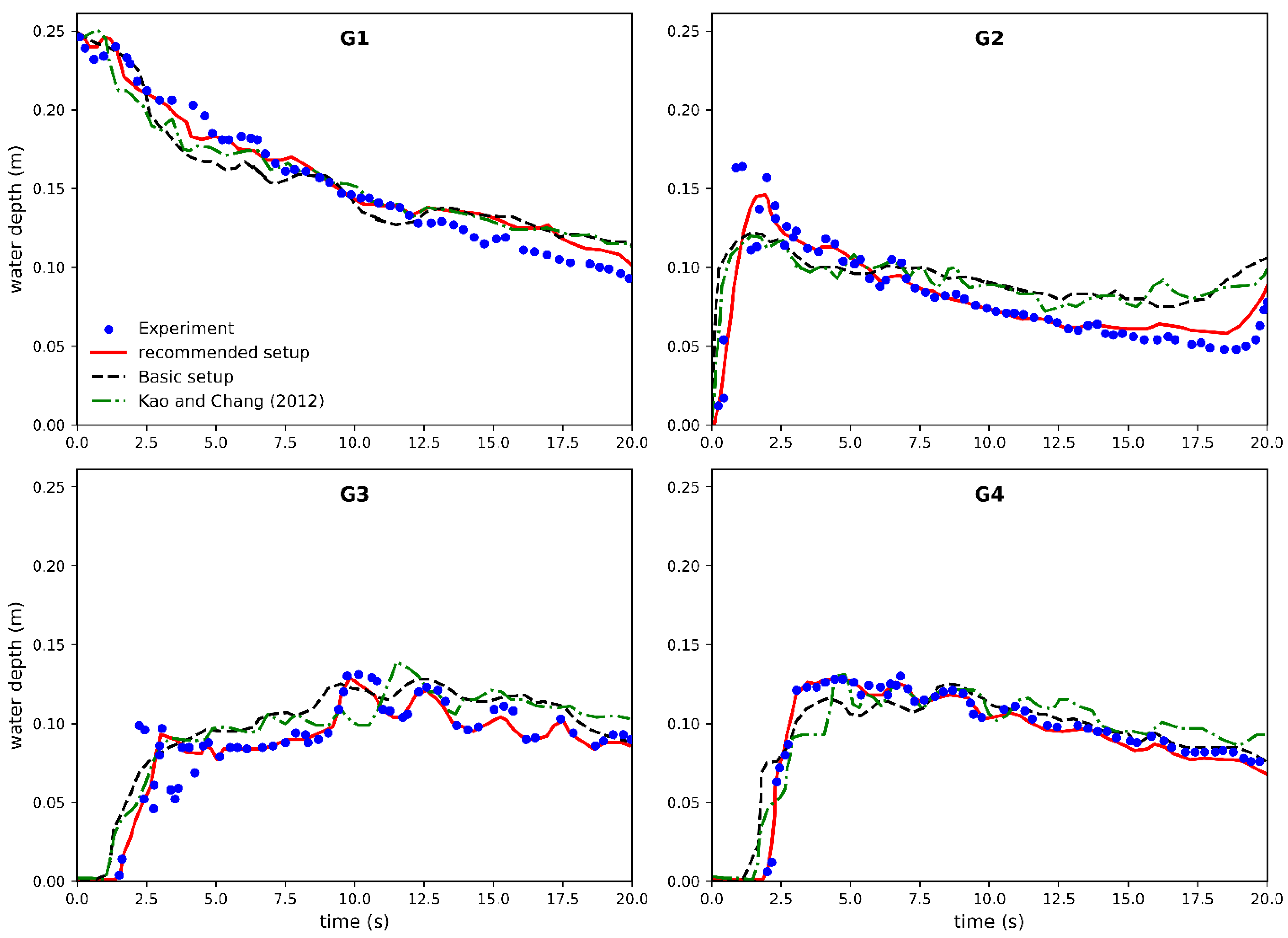
The comparison between the simulated and experimental water depths at the four gauges over a total simulation time of 20 s under the recommended setup, the basic setup, and the results from Kao and Chang [16] is presented in Figure 17. At early times (t < 2.5), the recommended setup showed closer agreement with the experimental water depth response than the basic setup and the results of Kao and Chang [16]. It also better reproduced the oscillatory behaviors observed at G3 after t = 10 s and at G4 after t = 7.5 s.

To quantify the agreement, a relative $L_2$ metric was employed, defined as

$$L_2=\sqrt{{\displaystyle \frac{1}{N}}{\displaystyle \sum _{i=1}^N}{\left({\displaystyle \frac{{h^{\prime }}_{i\left(SPH\right)}-{h^{\prime }}_{i\left(Exp\right)}}{{h^{\prime }}_{i\left(Exp\right)}}}\right)}^2},$$

(20)

where ${h^{\prime }}_{i \left(SPH\right)}$ and ${h^{\prime }}_{i \left(Exp\right)}$ represent the simulated and experimental water depths, respectively. The computed values for each gauge are summarized in

Table 7. $L_2$ errors between the simulated and experimental water depths for different setups.

Measurement Gauge	${\mathit{L}}_2$_Recommended Setup	${\mathit{L}}_2$_Basic Setup	${\mathit{L}}_2$_Kao and Chang [16]
G1	0.052	0.086	0.077
G2	0.175	0.497	0.347
G3	0.148	0.171	0.155
G4	0.111	0.269	0.154

. For the recommended setup, at G1—corresponding to the region where the flow varies smoothly—a low value of 0.052 was obtained. At G2 and G3—which correspond to the region of rapid flow transition immediately downstream of the gate and along the straight channel—larger errors of 0.175 and 0.148 were obtained, respectively. At G4—located in the bend section—the error decreased to 0.111, showing that the model maintained a consistent prediction after the flow entered the curved region. According to Kao and Chang (2012), error values below 0.2 indicate good agreement with experimental data [16].

5. Discussion

In this study, a parametric analysis was carried out to evaluate the influence of five numerical parameters on SPH simulations of dam-break flows. The results demonstrated that decreasing r leads to convergence of wave profiles, with minimal differences observed for r ≤ 2 m. Further refinement beyond this resolution provided negligible improvements in accuracy while increasing the computational cost. The optimal particle spacing reported for a previous 2D SPH dam-break benchmark corresponded to r/H ≈ 0.017, which is close to the value obtained in the present study (r/H ≈ 0.021) [36].

When q was set between 0.5 and 1, the results were closer to a unified wave profile. Similar observations are reported in [36], where the value of q is identified as 0.7. This falls within the range of 0.5 to 1 identified in this study. Moreover, the optimal value of q = 0.9 reported by Korzani et al. [37] is consistent with the range of 0.5 to 1 identified in the present study. In addition, their reported instability at q = 1.12 supports the conclusion that values outside this range may reduce the reliability of SPH simulations.

The computational runtime was nearly the same for all tested α values. Based on the results of this study, and consistent with two independent references [36,65], α values between 0.2 and 0.3 can be recommended for SPH simulations of dam-break flows. Zeng et al. [36] demonstrated that α = 0.19 provided the best results for dam-break flows, which is close to the lower end of the range identified in this study; however, they tested only a limited set of values, with the next tested value being α = 0.4, which introduced excessive damping. It is possible that, if they had tested additional values within the range of 0.2 to 0.3, they may have reported results consistent with those presented here.

The limited influence of α on the predicted WSE is not restricted to the Cleveland Dam configuration. The first-order Sobol’ index of α remained between 0.035 and 0.045 for the three dam heights considered (Table 3), and its second-order interactions with the other parameters were all close to zero (Table 4), which indicates that the small contribution of α to the variance of the WSE is preserved as the scale of the problem changes. This behavior is expected for dam-break flows, in which the free-surface response is governed primarily by gravity, inertia, and the bed topography, such that the small numerical dissipation introduced within the range of α = 0.2 to 0.3 does not appreciably alter the wave profile. The influence of α is therefore expected to remain limited for dam-break scenarios with comparable flow characteristics, whereas it may become more significant for flows in which viscous dissipation plays a larger role or for α values outside the tested range, where unphysical oscillations or excessive damping occur, as detailed in Section 3.1.

Previous dam-break benchmark and CFD studies have reported RMSE values of approximately 0.01–0.10 and R² values up to about 0.96 [12,13]. In the present SPH verification, the RMSE values (Table 6) remained consistently below 0.04 for all dimensionless times considered, while the corresponding R² values exceeded 0.98 for all examined times. The present model’s accuracy was within—and, in several cases, above—the range of values reported in comparable dam-break studies.

The L2 errors in Table 7 show that the recommended setup achieved the closest agreement with the experimental data for the 3D bend-channel test case. Lower errors were observed across all gauges, indicating that the selected numerical parameter ranges improve the consistency of the predicted water depths. Beyond the gauge-by-gauge comparison, this result demonstrates that the recommended numerical parameter ranges remain suitable for a case involving flow turning and three-dimensional propagation, where local water depth variations are more difficult to reproduce.

6. Conclusions

This study investigated the effects of selected SPH numerical parameters on WSE predictions for dam-break flood simulation over a LiDAR-derived computational domain. The unsteady incompressible Euler flow equations, SPH discretization, boundary treatment, and time-integration schemes were first presented to define the numerical framework and identify the parameters examined in the study. The initial numerical setup for the Cleveland Dam was then established, and the effects of the interparticle distance, smoothing length, time-stepping scheme, artificial viscosity coefficient, and kernel function were evaluated through a parametric study. The results revealed that a particle spacing of 2 m, corresponding to 298,188 particles, provides a suitable resolution for the present case, while the smoothing length ratio q should remain within the range of 0.5 to 1. The Symplectic scheme was adopted for the following simulations, based on its numerical properties. The artificial viscosity coefficient showed limited influence within the range of 0.2 to 0.3, and the cubic spline and Wendland kernels were found to produce comparable WSE responses.

The sensitivity analysis further demonstrated that the smoothing length is the dominant source of variability in WSE, followed by the kernel function, while the artificial viscosity coefficient has only a limited influence within the tested range. Based on the identified parameter ranges, a recommended setup was applied to the three-dimensional Cleveland Dam simulation to examine flood propagation and assess the resulting WSE patterns over the LiDAR-derived computational domain. The verification results supported the selected parameter ranges, as the SPH results showed close agreement with the calibrated HEC-RAS model at 80 m downstream. Furthermore, testing on a 2D dam-break benchmark yielded low RMSE values and high R² values, while the recommended setup achieved lower L2 errors in a 3D bend-channel test case when compared to the basic setup. These findings collectively indicate that the recommended SPH parameter ranges can improve the consistency of WSE predictions in dam-break flood simulations.

In future work, particular attention should be given to calibration of the smoothing length, as it exhibited the strongest influence on the simulation results in the present study. A systematic investigation of smoothing length selection may improve the robustness and reliability of SPH simulations across different flow conditions. Further studies could consider alternative evaluation metrics, such as discharge rates, to provide better insight into flood dynamics beyond WSE. Additionally, the presented verification could be extended to documented dam-break events at hydraulic structures with comparable configurations, which would further strengthen the practical applicability of the recommended parameter ranges to engineering practice.

References

- Xu, X.; Jiang, Y.-L.; Yu, P. SPH simulations of 3D dam-break flow against various forms of the obstacle: Toward an optimal design. Ocean Eng. 2021, 229, 108978. [Google Scholar] [CrossRef] [Scilit]
- Flood, M. Laser altimetry: From science to commerical lidar mapping. Photogramm. Eng. Remote Sens. 2001, 67, 1209–1218. [Google Scholar]
- Peramuna, P.; Neluwala, N.; Wijesundara, K.; DeSilva, S.; Venkatesan, S.; Dissanayake, P. Review on model development techniques for dam break flood wave propagation. Wiley Interdiscip. Rev. Water 2024, 11, e1688. [Google Scholar]
- Bales, J.D.; Wagner, C.R.; Tighe, K.C.; Terziotti, S. LiDAR-Derived Flood-Inundation Maps for Real-Time Flood-Mapping Applications, Tar River Basin, North Carolina; Geological Survey (US): Reston, VA, USA, 2007.
- Maranzoni, A.; Tomirotti, M. Three-dimensional numerical modelling of real-field dam-break flows: Review and recent advances. Water 2023, 15, 3130. [Google Scholar] [CrossRef] [Scilit]
- Brufau, P.; Vázquez-Cendón, M.E.; García-Navarro, P. A numerical model for the flooding and drying of irregular domains. Int. J. Numer. Methods Fluids 2002, 39, 247–275. [Google Scholar] [CrossRef] [Scilit]
- Teng, J.; Jakeman, A.J.; Vaze, J.; Croke, B.F.; Dutta, D.; Kim, S. Flood inundation modelling: A review of methods, recent advances and uncertainty analysis. Environ. Model. Softw. 2017, 90, 201–216. [Google Scholar] [CrossRef] [Scilit]
- Bates, P.D. Flood inundation prediction. Annu. Rev. Fluid Mech. 2022, 54, 287–315. [Google Scholar] [CrossRef] [Scilit]
- Toro, E.F.; Garcia-Navarro, P. Godunov-type methods for free-surface shallow flows: A review. J. Hydraul. Res. 2007, 45, 736–751. [Google Scholar] [CrossRef] [Scilit]
- Castro-Orgaz, O.; Hager, W.H. Shallow Water Hydraulics; Springer: Berlin/Heidelberg, Germany, 2019. [Google Scholar]
- Brunner, G.W. HEC-RAS Hydraulic Reference Manual, Version 5.0; US Army Corps of Engineers, Hydrologic Engineering Center: Davis, CA, USA, 2016.
- Magdalena, I.; Pebriansyah, M.F.E. Numerical treatment of finite difference method for solving dam break model on a wet-dry bed with an obstacle. Results Eng. 2022, 14, 100382. [Google Scholar] [CrossRef] [Scilit]
- Ferdowsi, A.; Nemati, M.; Farzin, S. Development of dam-break model considering real case studies with asymmetric reservoirs. Comput. Eng. Phys. Model. 2021, 4, 39–63. [Google Scholar]
- Kleefsman, K.; Fekken, G.; Veldman, A.; Iwanowski, B.; Buchner, B. A volume-of-fluid based simulation method for wave impact problems. J. Comput. Phys. 2005, 206, 363–393. [Google Scholar] [CrossRef] [Scilit]
- Marsooli, R.; Wu, W. 3-D finite-volume model of dam-break flow over uneven beds based on VOF method. Adv. Water Resour. 2014, 70, 104–117. [Google Scholar] [CrossRef] [Scilit]
- Kao, H.-M.; Chang, T.-J. Numerical modeling of dambreak-induced flood and inundation using smoothed particle hydrodynamics. J. Hydrol. 2012, 448, 232–244. [Google Scholar] [CrossRef] [Scilit]
- Xu, X.; Ouyang, J.; Jiang, T.; Li, Q. Numerical analysis of the impact of two droplets with a liquid film using an incompressible SPH method. J. Eng. Math. 2014, 85, 35–53. [Google Scholar]
- Fürstenau, J.-P.; Weißenfels, C.; Wriggers, P. Free surface tension in incompressible smoothed particle hydrodynamcis (ISPH). Comput. Mech. 2020, 65, 487–502. [Google Scholar]
- Monaghan, J.J. Simulating free surface flows with SPH. J. Comput. Phys. 1994, 110, 399–406. [Google Scholar] [CrossRef] [Scilit]
- Marrone, S.; Antuono, M.; Colagrossi, A.; Colicchio, G.; Le Touzé, D.; Graziani, G. δ-SPH model for simulating violent impact flows. Comput. Methods Appl. Mech. Eng. 2011, 200, 1526–1542. [Google Scholar] [CrossRef] [Scilit]
- Lucy, L.B. A numerical approach to the testing of the fission hypothesis. Astron. J. 1977, 82, 1013–1024. [Google Scholar] [CrossRef] [Scilit]
- Gingold, R.A.; Monaghan, J.J. Smoothed particle hydrodynamics: Theory and application to non-spherical stars. Mon. Not. R. Astron. Soc. 1977, 181, 375–389. [Google Scholar] [CrossRef] [Scilit]
- Wang, L.; Xu, F.; Yang, Y. SPH scheme for simulating the water entry of an elastomer. Ocean Eng. 2019, 178, 233–245. [Google Scholar] [CrossRef] [Scilit]
- Yang, Q.; Xu, F.; Yang, Y.; Wang, J. Two-phase SPH model based on an improved Riemann solver for water entry problems. Ocean Eng. 2020, 199, 107039. [Google Scholar] [CrossRef] [Scilit]
- Lin, Y.; Liu, G.; Wang, G. A particle-based free surface detection method and its application to the surface tension effects simulation in smoothed particle hydrodynamics (SPH). J. Comput. Phys. 2019, 383, 196–206. [Google Scholar] [CrossRef] [Scilit]
- Artkeli Farahani, M.; Morency, F. Urban Flood Mapping Using SPH Method and Precipitation Data Based on LiDAR Data. In Proceedings of the 16th World Congress on Computational Mechanics and 4th Pan American Congress on Computational Mechanics (WCCM-PANACM), Vancouver, BC, Canada, 21–26 July 2024. [Google Scholar]
- Xu, J.; Zhang, Y.; Ma, Q.; Zhang, J.; Hu, Q.; Zhan, Y. Dam-Break Hazard Assessment with CFD Computational Fluid Dynamics Modeling: The Tianchi Dam Case Study. Water 2025, 17, 108. [Google Scholar] [CrossRef] [Scilit]
- Bo, H.; Zhang, F.; Zhang, L.; Zhang, X.; Yin, L. The Effect of Dam Break Speed on Flood Evolution in a Downstream Reservoir of a Cascade Reservoir System. Water 2024, 16, 2993. [Google Scholar] [CrossRef] [Scilit]
- Zhang, J.; Wang, B.; Li, H.; Zhang, F.; Wu, W.; Hu, Z.; Deng, C. Progressive Dam-failure assessment by smooth particle hydrodynamics (SPH) method. Water 2023, 15, 3869. [Google Scholar] [CrossRef] [Scilit]
- Artkeli Farahani, M.; Morency, F. Mapping of an Urban Flood Caused by a Dam Break Using SPH Method Based on LiDAR Data. In Proceedings of the Canadian Society for Mechanical Engineering International Congress and 31st Annual Conference of the Computational Fluid Dynamics Society of Canada (CSME/CFD2024), Toronto, ON, Canada, 26–29 May 2024. [Google Scholar]
- Farahani, M.A.; Morency, F. Effects of numerical and physical parameters on SPH models using LiDAR-based dam-break flood simulations. In Proceedings of the Communication lors de la Conférence: CSME-CFDSC-CSR 2025 International Congress, Montreal, QC, Canada, 25–28 May 2025. [Google Scholar]
- Crespo, A.J.; Domínguez, J.M.; Rogers, B.D.; Gómez-Gesteira, M.; Longshaw, S.; Canelas, R.; Vacondio, R.; Barreiro, A.; García-Feal, O. DualSPHysics: Open-source parallel CFD solver based on Smoothed Particle Hydrodynamics (SPH). Comput. Phys. Commun. 2015, 187, 204–216. [Google Scholar] [CrossRef] [Scilit]
- Domínguez, J.M.; Fourtakas, G.; Altomare, C.; Canelas, R.B.; Tafuni, A.; García-Feal, O.; Martínez-Estévez, I.; Mokos, A.; Vacondio, R.; Crespo, A.J. DualSPHysics: From fluid dynamics to multiphysics problems. Comput. Part. Mech. 2022, 9, 867–895. [Google Scholar] [CrossRef] [Scilit]
- DualSPHysics Website. Available online: https://dual.sphysics.org/ (accessed on 22 July 2026).
- Crespo, A.J.C. DualSPHysics Wiki. 2023. Available online: https://github.com/DualSPHysics/DualSPHysics/wiki/3.-SPH-formulation (accessed on 22 July 2026).
- Zeng, J.; Shen, J.; Liu, H. A Parametric Study of Dam Break Flow Feature over a Dry Bed Using SPH Modeling. In Proceedings of the 10th International Conference on Asian and Pacific Coasts (APAC 2019), Hanoi, Vietnam, 25–28 September 2019. [Google Scholar]
- Korzani, M.G.; Galindo-Torres, S.A.; Scheuermann, A.; Williams, D.J. Parametric study on smoothed particle hydrodynamics for accurate determination of drag coefficient for a circular cylinder. Water Sci. Eng. 2017, 10, 143–153. [Google Scholar] [CrossRef] [Scilit]
- Monaghan, J.J. Smoothed particle hydrodynamics. Annu. Rev. Astron. Astrophys. 1992, 30, 543–574. [Google Scholar] [CrossRef]
- Liu, G.-R.; Liu, M.B. Smoothed Particle Hydrodynamics: A Meshfree Particle Method; World Scientific: Singapore, 2003. [Google Scholar]
- Monaghan, J.J. Smoothed Particle Hydrodynamics. Rep. Prog. Phys. 2005, 68, 1703. [Google Scholar] [CrossRef] [Scilit]
- Violeau, D. Fluid Mechanics and the SPH Method: Theory and Applications; Oxford University Press: Oxford, UK, 2012. [Google Scholar]
- Monaghan, J.J.; Lattanzio, J.C. A refined particle method for astrophysical problems. Astron. Astrophys. 1985, 149, 135–143. [Google Scholar]
- Wendland, H. Piecewise polynomial, positive definite and compactly supported radial functions of minimal degree. Adv. Comput. Math. 1995, 4, 389–396. [Google Scholar] [CrossRef] [Scilit]
- Gomez-Gesteira, M.; Rogers, B.D.; Dalrymple, R.A.; Crespo, A.J. State-of-the-art of classical SPH for free-surface flows. J. Hydraul. Res. 2010, 48, 6–27. [Google Scholar] [CrossRef] [Scilit]
- English, A.; Domínguez, J.; Vacondio, R.; Crespo, A.; Stansby, P.; Lind, S.; Chiapponi, L.; Gómez-Gesteira, M. Modified dynamic boundary conditions (mDBC) for general-purpose smoothed particle hydrodynamics (SPH): Application to tank sloshing, dam break and fish pass problems. Comput. Part. Mech. 2022, 9, 911–925. [Google Scholar] [CrossRef] [Scilit]
- Dalrymple, R.A.; Knio, O. SPH modelling of water waves. In Coastal Dynamics’01; American Society of Civil Engineers: Reston, VA, USA; pp. 779–787.
- Cabrera Crespo, A.J.; Gómez Gesteira, R.; Dalrymple, R.A. Boundary conditions generated by dynamic particles in SPH methods. Comput. Mater. Contin. 2007, 5, 173–184. [Google Scholar]
- Domínguez, J.; Fourtakas, G.; Cercós-Pita, J.; Vacondio, R.; Rogers, B.D.; Crespo, A. Evaluation of reliability and efficiency of different boundary conditions in a SPH code. In Proceedings of the 10th International SPHERIC Workshop, Parma, Italy, 16–18 June 2015. [Google Scholar]
- Liu, M.; Liu, G.-R. Restoring particle consistency in smoothed particle hydrodynamics. Appl. Numer. Math. 2006, 56, 19–36. [Google Scholar] [CrossRef] [Scilit]
- Monaghan, J. On the problem of penetration in particle methods. J. Comput. Phys. 1989, 82, 1–15. [Google Scholar] [CrossRef] [Scilit]
- Leimkuhler, B.J.; Reich, S.; Skeel, R.D. Integration methods for molecular dynamics. In Mathematical Approaches to Biomolecular Structure and Dynamics; Springer: Berlin/Heidelberg, Germany, 1996; pp. 161–185. [Google Scholar]
- Parshikov, A.N.; Medin, S.A.; Loukashenko, I.I.; Milekhin, V.A. Improvements in SPH method by means of interparticle contact algorithm and analysis of perforation tests at moderate projectile velocities. Int. J. Impact Eng. 2000, 24, 779–796. [Google Scholar] [CrossRef] [Scilit]
- Corporation of the District of North Vancouver. Available online: https://www.dnv.org/programs-and-services/upper-capilano (accessed on 22 July 2026).
- Dunphy, M. Available online: https://www.straight.com/news/three-workers-fired-in-aftermath-of-cleveland-dam-incident-that-resulted-in-one-dead-one (accessed on 22 July 2026).
- GIS Website. Available online: https://desktop.arcgis.com/en/arcmap/latest/manage-data/las-dataset/what-is-a-las-dataset-.htm (accessed on 22 July 2026).
- Bernardini, F.; Mittleman, J.; Rushmeier, H.; Silva, C.; Taubin, G. The ball-pivoting algorithm for surface reconstruction. IEEE Trans. Vis. Comput. Graph. 1999, 5, 349–359. [Google Scholar] [CrossRef] [Scilit]
- Google LLC. Google Earth Pro, Version 7.3.6: Cleveland Dam and the Surrounding Capilano River Valley, North Vancouver, BC, Canada. Available online: https://www.google.com/earth/about/versions/ (accessed on 15 December 2024).
- Price, D.J.; Monaghan, J.J. Smoothed Particle Magnetohydrodynamics—II. Variational principles and variable smoothing-length terms. Mon. Not. R. Astron. Soc. 2004, 348, 139–152. [Google Scholar] [CrossRef] [Scilit]
- Ardıçlıoğlu, M.; Kuriqi, A. Calibration of channel roughness in intermittent rivers using HEC-RAS model: Case of Sarimsakli creek, Turkey. SN Appl. Sci. 2019, 1, 1080. [Google Scholar] [CrossRef] [Scilit]
- Dhote, P.R.; Bansal, J.K.; Garg, V.; Thakur, P.K.; Agarwal, A. A framework for generating rating curves in Mahanadi River using hydrodynamic model and radar altimetry data. Hydrol. Sci. J. 2025, 70, 390–405. [Google Scholar] [CrossRef] [Scilit]
- Attari, M.; Hosseini, S.M. A simple innovative method for calibration of Manning’s roughness coefficient in rivers using a similarity concept. J. Hydrol. 2019, 575, 810–823. [Google Scholar] [CrossRef] [Scilit]
- Bessar, M.A.; Matte, P.; Anctil, F. Uncertainty analysis of a 1d river hydraulic model with adaptive calibration. Water 2020, 12, 561. [Google Scholar] [CrossRef] [Scilit]
- Moriasi, D.N.; Arnold, J.G.; Van Liew, M.W.; Bingner, R.L.; Harmel, R.D.; Veith, T.L. Model evaluation guidelines for systematic quantification of accuracy in watershed simulations. Trans. ASABE 2007, 50, 885–900. [Google Scholar] [CrossRef] [Scilit]
- Moriasi, D.N.; Gitau, M.W.; Pai, N.; Daggupati, P. Hydrologic and water quality models: Performance measures and evaluation criteria. Trans. ASABE 2015, 58, 1763–1785. [Google Scholar] [CrossRef] [Scilit]
- Fraga Filho, C.A.D. Smoothed Particle Hydrodynamics; Springer: Berlin/Heidelberg, Germany, 2019. [Google Scholar]
- Dal, K.; Evangelista, S.; Yilmaz, A.; Kocaman, S. Validation of dam-break problem over dry bed using SPH. Int. J. Adv. Eng. Res. Sci. 2017, 4, 237350. [Google Scholar] [CrossRef] [Scilit]
- Kocaman, S. Experimental and Theoretical Investigation of Dam-Break Problem; University of Cukurova Adana: Adana, Turkey, 2007. [Google Scholar]
- Morris, M. Concerted Action on Dambreak Modelling – CADAM; Project Report; HR Wallingford Ltd.: Wallingford, UK, 2000. [Google Scholar]
- Frazao, S.S.; Zech, Y. Effects of a sharp bend on dam-break flow. In Proceedings of the 28th Congress of IAHR, Graz, Austria, 22–27 August 1999; pp. 1–20. [Google Scholar]
Disclaimer/Publisher’s Note: The statements, opinions and data contained in all publications are solely those of the individual author(s) and contributor(s) and not of MDPI and/or the editor(s). MDPI and/or the editor(s) disclaim responsibility for any injury to people or property resulting from any ideas, methods, instructions or products referred to in the content. |
© 2026 by the authors. Licensee MDPI, Basel, Switzerland. This article is an open access article distributed under the terms and conditions of the Creative Commons Attribution (CC BY) license.