


Highlights
What are the main findings?
- Seasonal vegetation dynamics differed between urban and natural habitats and were associated with the peak of wild boar urban presence.
- Landscape connectivity (streams) and fragmentation, rather than vegetation indices, explained spatial variation in urban green area use.
What are the implications of the main findings?
- Urban wild boar presence appears to arise from multi-scale processes, where temporal resource dynamics and spatial structure interact. Combining remote sensing with landscape metrics may improve predictions of when incursions occur and where they are more likely.
- Management should prioritise highly connected urban areas and reduce resource attractiveness in key entry points.
Abstract
Urbanisation is reshaping ecosystems and increasing human–wildlife interactions. Wild boar (Sus scrofa), a highly adaptable species, is increasingly common in European cities, where it exploits natural and anthropogenic resources, often leading to conflict. Predicting when and where wild boars enter urban areas remains challenging, particularly using scalable tools such as remote sensing. Here, we show that temporal and spatial drivers of urban presence are decoupled in Barcelona over a 14-year period. Seasonal vegetation dynamics influenced the timing of urban incursions, with peaks in spring and late summer associated with changes in vegetation moisture and likely reinforced by increased energetic demands during reproduction and early lactation. However, remotely sensed vegetation indices captured these dynamics only partially, limiting their predictive power when used alone. Spatial variation in urban green area use was primarily explained by landscape structure, with proximity to streams and habitat fragmentation contributing similarly. Green areas near natural corridors were concentrated higher and had more variable presence, while heterogeneous landscapes likely facilitated repeated use by increasing access to foraging and refuge. Integrating remote sensing with landscape metrics can improve the anticipation and management of human–wildlife conflicts.
1. Introduction
Human-driven environmental changes affect ecosystems across the globe [1]. Among these changes, urbanisation stands out as a dominant trend. Urban areas currently account for approximately 3% of the total land area of Earth, and yet they contain about half of the world’s human population [2], a figure expected to peak in the 2080s [3]. This expansion alters land use and disrupts ecological processes, leading to biotic and genetic homogenisation [4,5,6,7]. Altogether, urban settlements expand into natural areas, reducing the habitat availability for wildlife [8], which must adapt their life cycles to the new scenario, relocate, or disappear [9].
Despite its ecological impacts, urbanisation has also created novel opportunities for highly adaptable and generalist species [10,11,12]. In Europe, for instance, wild boars (Sus scrofa) and medium-sized carnivores such as red foxes (Vulpes vulpes) and Eurasian badgers (Meles meles) successfully exploit these urban habitats [8,13]. Synurbic wildlife may not reside permanently in cities but benefit from the refuge and resources in urbanised areas, particularly those close to peri-urban natural habitats or green spaces [8,13,14].
Wild boar has become a leading example of urban wildlife adaptation [15,16,17]. This mammal is characterised by the highest reproductive rate among ungulates and a broad ecological, demographic, and behavioural flexibility [18,19]. These traits, coupled with broad environmental and socio-economic changes, such as rural abandonment, shifts in crop types, milder winters, and declining predator and hunting pressures, have supported its expansion into urban habitats [20,21,22]. Wild boars have increasingly established synurbic populations across European cities, where they behave as urban exploiters [15,16,23,24,25,26,27]. This has heightened the reciprocal habituation with humans, leading to increased interactions and conflicts [15,28,29,30], including traffic accidents, aggressions, damage to green areas and infrastructure, and increased zoonotic disease risk [31,32,33,34,35,36].
In urban environments, synurbic wild boars exploit anthropogenic food sources such as garbage, pet food, or intentional feeding by humans [16,29]. They also actively seek urban green areas and areas of high vegetation productivity throughout the year [17,33,37,38], which can offer shelter, food, and water [15]. Nevertheless, they may remain ecologically tied to forested habitats and show a strong preference for natural food resources and landscapes [23,39,40,41,42]. Seasonal events, such as spring and summer farrowing or summer droughts (particularly intense in Mediterranean climates), trigger wild boar use of urban areas in search of food and water [16,24,43,44]. The spatial behaviour and daily activities of wild boars in urban environments are shaped by human disturbances, landscape structure, and the distribution of resources [17,24,33,38,42,45,46].
In Barcelona, the wild boar population inhabiting Collserola Natural Park (CNP) has increased tenfold over the last 20 years [44]. The CNP is largely isolated from other natural areas due to intense infrastructure pressure on its periphery [43,47], and the CNP wild boars maintain reduced genetic flow with neighbouring populations [26]. Therefore, during the summer natural resource scarcity period, wild boar presence increases in urban landscapes [16,24]. To manage this growing challenge, local authorities have been allocating increasing amounts of public resources to different strategies [48,49,50,51]. These include reducing the attractiveness of the city, limiting anthropogenic food resources, conducting vegetation clearings in the urban-forest ecotone, reducing population numbers, and raising public awareness [52]. Despite these efforts, effectively anticipating wild boar presence and managing conflicts in such complex and dynamic urban contexts remains challenging.
Statistical models have been developed to predict wild boar presence and human–wildlife conflicts (HWCs) across rural and peri-urban landscapes [24,34,46,53,54]. These models typically incorporate environmental factors such as proximity to natural habitats, landscape structure, and resource distribution. However, the role of primary production in predicting wild boar occurrence has only been limitedly investigated in rural or agricultural contexts, but not in urban and peri-urban settings [41,55].
Satellite remote sensing (SRS) is a cost-effective, long-term monitoring tool that can provide consistent data on vegetation dynamics [56]. Vegetation indices (VIs) derived from spectral reflectance data include the normalised difference vegetation index (NDVI), enhanced vegetation index (EVI), normalised difference water index (NDWI), and global vegetation moisture index (GVMI), which reflect primary production, vegetation health, and water content in both vegetation and soil [57,58,59,60,61]. These indices are widely applied in agriculture and conservation to infer ecological processes and habitat conditions [56,62,63]. However, the use of vegetation indices for predicting urban wildlife conflict remains limited, with few studies focusing on large mammals in urban environments [37]. Thus, a significant gap remains in integrating remotely sensed vegetation indices (RS-VIs) with predictive models for addressing wild boar-related conflicts in complex urban contexts. The present study evaluates the relationship between wild boar occurrence in Barcelona and multiple RS-VIs across both natural and urban green areas. Additionally, given the need for fine-scale ecological understanding [17], the study also identifies the urban green area characteristics best predicting wild boar presence. We hypothesised that RS-VIs could serve as a cost-effective and scalable tool to anticipate conflict hotspots and inform adaptive management for improved planning and resource allocation. Finally, we predicted that due to continuous irrigation, RS-VI values in urban parks would be higher than those of the CNP during the summer scarcity period, which would help explain the occurrence of wild boar presence in urban settings.
2. Materials and Methods
2.1. Study Area and Plot Selection
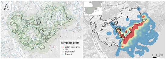
The study area included the CNP and 32 urban parks and green areas (hereafter “green areas”) located in the Barcelona districts bordering the Collserola massif (Figure 1). This massif covers approximately 11,100 ha, including the 8295 hectares of the CNP [64]. The relief is gentle and asymmetrical, with ridges facing inland, long and gently sloping, and short and steep slopes facing the sea.
Figure 1.
(Left): Map of the study area showing the sampling points for remotely sensed vegetation indices (RS-VIs) in Collserola Natural Park (CNP; green dots) and in Barcelona urban green areas (red dots). The urban green areas located within a 1 km buffer from the CNP boundary (green shading) were included in the PLSR analysis. (Right): Kernel density map of wild boar-related incidences in Barcelona, supporting the selection of urban green areas within the buffer zone as focal areas for analysis. Colours represent relative kernel density values, ranging from low (blue) to high (red) concentrations of wild boar presences.
Collserola has a typical Mediterranean climate, with an average annual temperature of 14 °C. Winters are generally mild, with temperatures typically above 5 °C, while summers are hot and dry, with an average temperature of 21 °C. Spring and autumn are transition seasons characterised by concentrated and irregular rainfall. These two seasons constitute the two wet periods, with an average rainfall of 83.1 mm in October and 60.4 mm in May, followed by intense summer drought in July (10.6 mm). Despite these generalities, there are significant local climatic variations, influenced by the topography, the thermoregulatory effect of the sea, altitudinal variations, the sun exposure on the slopes, and the vegetation cover, among others [65].
The landscape consists of a complex, dynamic mosaic of natural habitats, with meadows, grasslands, scrublands, and croplands, predominated by Mediterranean forests. The most abundant forest type is a mixed woodland of Holm oaks (Quercus ilex) with an upper canopy of Aleppo pine (Pinus halepensis) and interspersed Quercus × cerrioides. The Holm oak woodland is a dense and humid forest further characterised by a tall shrub stratum (1.5–3 m) and a whole host of creeping and climbing plants that sometimes make the wood impenetrable. Secondary pine forests, dominated by Aleppo pine with smaller numbers of stone pine (Pinus pinea), normally occupy abandoned farmland. In this habitat, oaks are also found among the pines, which also have an undergrowth consisting of plants from open environments, like cistus (Cistus spp.), rosemary (Rosmarinus officinalis) and gorse (Ulex parviflorus) [64].
We selected the urban green areas that met two criteria: (1) previously reported wild boar presence, and/or (2) the existence of irrigation systems to maintain green spaces and vegetation during the dry summer months. These green areas differ in vegetation, size, and proximity to the CNP.
We selected one sampling plot in each urban green area with a minimum width of 30 m to minimise interference from paths, concrete, and bare soil. In the CNP, we selected 1492 sampling plots representing nine land cover types from the 41 categories in the ICGC (Institut Cartogràfic i Geològic de Catalunya) land cover dataset, focusing on natural and agricultural areas. Pine and oak forests were excluded since EVI and NDVI are not reliable indicators of leaf photosynthetic rates or drought events in evergreen Mediterranean forests [66,67]. We defined each sampling location as a 30 m-side pixel (corresponding to 900 m2) matching the native spatial resolution of the Landsat surface reflectance product. Spatial geoprocessing was conducted in QGIS 3.10.0 [68].
2.2. Wild Boar Presence
Wild boar presence refers to at least one alive, wounded, or dead wild boar in the city of Barcelona [24]. These were reported by citizens to the local police of Barcelona, who registered the location, date, and time of each event. Therefore, they represent observed and reported urban presence events, rather than a complete measure of habitat-use intensity. To avoid pseudo-replication, we processed these data, retaining only one presence if multiple events occurred within a 500 m buffer in a two-hour timeframe, following Castillo-Contreras et al. [24]. From 2010 to 2024, we registered a total of 8321 refined presences.
2.3. Satellite Images and Extraction of Vegetation Indices
To characterise the vegetation dynamics, we obtained surface reflectance Landsat imagery through Google Earth Engine [69]. We selected images based on their availability and temporal coverage of the study area, covering the period from 2010 to 2024. The datasets, accessible under the LANDSAT/LT05/C02/T1_L2, LANDSAT/LE07/C02/T1_L2, and LANDSAT/LC08/C02/T1_L2 collections, provide atmospherically corrected surface reflectance products standardised under the Collection 2 framework [70,71,72]. The Collection 2 framework ensures high geometric accuracy, radiometric calibration, and consistent preprocessing across different Landsat missions, facilitating reliable multi-temporal and cross-sensor comparisons.
We filtered the imagery to match the extent of our study area using a custom shapefile. The images were clipped to this region and exported as multispectral images with a spatial resolution of 30 m. These geoprocessing steps were automated through a custom Earth Engine script. Only images with minimal cloud cover were considered, and further cloud masking steps were performed during subsequent preprocessing stages. Further imagery processing was conducted in R statistical software version 4.3.1 [73]. We used the “terra” package [74] over a polygon shapefile delimiting the sampling plots to combine the different spectral bands from the images and generate vegetation indices. These included NDVI [57], EVI2 [75] (Enhanced Vegetation Index 2, equivalent to EVI from modern sensors), NDWI [58], and GVMI [59,60,76]. EVI2 and NDVI are commonly used proxies of vegetation greenness and productivity [57,75], while NDWI and GVMI are more closely related to vegetation and canopy water content [58,59,60].
The most well-known VI, the NDVI, was used as a quality-control filter to remove anomalous reflectance values. Because all plots had been pre-selected as vegetated areas, we applied the widely accepted NDVI range of NDVI > 0.1 and NDVI < 1, consistent with established interpretations of NDVI values for vegetated areas [70,77]. Observations falling outside this range were interpreted as non-physical artefacts caused by sensor or atmospheric issues, such as cloud contamination, shadows, or striping errors typical of Landsat 7 ETM+ SLC-off data, rather than representing actual surface conditions. After correlation analysis confirming high correlation between EVI2 and NDVI, we selected EVI2 for further analyses because it is less sensitive to soil and atmospheric noise, and NDVI saturates in evergreen vegetation [78,79].
To obtain monthly VI values for each urban green area while minimising sensitivity to outliers, we first calculated the median. For the CNP, we explored EVI2 phenology across different land uses and aggregated them into four broader categories: arable land, permanent crops (olives and vineyards), scrubland, and meadows and pastures. For each of these new combined land-use categories, we also calculated the median VI values. Then, for both the urban green areas and CNP, we aggregated the data by averaging the monthly medians across individual green areas or land-use categories. This resulted in a single VI value per month for urban green areas and the CNP, which was subsequently used to construct harmonised and consistent regular time series (TS). We used linear interpolation between adjacent values as a gap-filling method to estimate missing VI data (two observations in the CNP and four observations in the urban green areas).
2.4. Statistical Analyses
All statistical analyses were conducted in R statistical software 4.3.1 [73].
2.4.1. Analysis of Long-Term Temporal Trends
To evaluate the long-term temporal trends and dynamics in both presence and VI in the urban green areas and CNP, we followed the protocol proposed by Verbesselt et al. [80] using the “bfast” analysis. BFAST, which stands for “Breaks For Additive Season and Trend”, detects and characterises “breakpoints” or structural changes in the time series (TS) by iteratively decomposing it into three different components: trend, seasonal, and remainder [80].
The analysis followed an iterative procedure, beginning with seasonal trend decomposition using the LOESS method (STL) [81]. STL subtracted the trend from the observed values, resulting in a detrended TS that represents seasonality alone (St). This detrended TS was then averaged to obtain a representative seasonal component. The remainder component (or noise) captured residual variation not explained by trend or seasonality. Afterwards, BFAST applied the ordinary least squares residuals-based moving sum test (OLS-MOSUM), which identified significant shifts or “breakpoints” in the trend component. Breakpoints were determined iteratively, minimising the Bayesian information criterion (BIC) and optimising their position through reduction of the residual sum of squares (RSS). This process was repeated until both the number and placement of breakpoints were stable.
BFAST transformed the TS into a piecewise linear regression model in which the maximum number of regressions was influenced by the parameter “h”. This parameter defines the minimum segment size between potential breaks in the trend model, expressed as a fraction of the total sample size [80]. By setting the minimum segment size, h determines the potential number of breaks [80,82]. For our analysis, each TS included 168 observations (14 years at a monthly frequency). We set the significant trend periods at h = 1/8 following the recommendations of Watts et al. [82] which corresponded to a minimum segment size of 21 observations (21 months), allowing for the detection of up to seven breakpoints.
After extracting the temporal and seasonal trends from the BFAST models, we investigated whether the long-term trends of VIs from the urban green areas, CNP, and wild boar presence were correlated. We obtained the predicted monthly values of the trend component (i.e., the piecewise model) from the BFAST models, and then conducted Kendall correlation analysis, since they are well-suited for handling ties. Additionally, to test whether the VI trends statistically predicted the presence trend, we fitted a set of linear models. We used the predicted number of presences as the response variable and the predicted VI of the CNP and urban green areas as the predictors. To account for autocorrelation, we applied Newey–West standard errors to adjust the inference [83].
2.4.2. Evaluation of the Relationship Between Seasonal Trends
To evaluate the relationship between VI seasonal variation and wild boar presence, we fitted generalised additive mixed models (GAMMs) using the “mgcv” package [84,85]. We fitted these seasonal models separately for the urban green areas and the CNP. The models included month as a cyclic smoothing function to account for seasonal patterns [86]. The maximum of knots was below the number of months to prevent model overfitting [86]. We included year as a random term to account for interannual variability. We used the Gaussian family with an identity link function for the VI, and Poisson family with log link for wild boar presence, or a negative binomial distribution if the model showed overdispersion. Subsequently, we assessed model fit using standard residual diagnostics following Zuur et al. [87] and Wood [85]. We conducted Levene’s test for homogeneity of variance [88] and tests for temporal autocorrelation (e.g., Durbin–Watson) using the “mgcViz” and “DHARMa” packages to validate the wild boar urban presence GAMM [89,90].
We then extracted the predicted values and standardised residuals. Predicted values represented within-year cyclic seasonal variation adjusted for interannual variability, whereas the residuals no longer contained the seasonal cycle, reflecting the unexplained variation. After exploring the residual distribution, we conducted Kendall correlation tests between the standardised residuals of the set of GAMMs. This analysis aimed to identify whether short-term anomalies (e.g., sudden droughts, unseasonal green-ups) in vegetation indices were linked to unexpected increases or decreases in wild boar presence. We repeated the correlations between the predicted values to compare the general seasonal co-fluctuation of vegetation indices and wild boar presence.
To quantify the relationship between monthly vegetation in the urban green areas and CNP and the presence of wild boar in urban areas, we fitted a set of generalised linear mixed models (GLMMs) using the glmmTMB package [91]. Monthly wild boar incidences were modelled as negative binomial counts with a log link to account for overdispersion. All models included year as a random intercept to account for interannual variability, and month as linear, quadratic, and cubic terms to represent seasonal dynamics identified in the preliminary GAMM exploration. The RS-VIs (EVI2, NDWI, GVMI) were included as predictors separately for the urban green areas (subscript p) and Collserola (subscript c). To improve interpretability and reduce collinearity, each index was centred before modelling. Since several indices were strongly correlated within habitat type, we compared a structured set of candidate models, including: (i) seasonality only, (ii) single-index models for each habitat, (iii) combined habitat models (e.g., GVMIc + GVMIp), (iv) a PCA-based model, using the first principal component from each habitat, (v) a Δ-model using differences between the urban green areas and the CNP (e.g., ΔEVI2 = EVI2p − EVI2c), (vi) a full model including all indices, and (vii) zero-inflated versions of the key models to account for potential excess zeros. The models were compared using AIC and AICc, and the model with the lowest AICc was selected as the best-supported model. Model assumptions were evaluated using DHARMa simulation-based diagnostics [90]. We assessed multicollinearity using variance inflation factors (VIFs), and model explanatory power was quantified using Nakagawa’s marginal and conditional R2 [92]. Partial effect plots were produced using the ggeffects package [93].
2.4.3. Evaluation of the Relationship Between Wild Boar Presence and Urban Green Area Characteristics
Finally, to identify local predictors for wild boar presence in the urban area of Barcelona, we evaluated the relationship between the number of presences during the peak period (May to October, n = 6189) and the values of the VIs and landscape metrics of each green area. Because most presences (5752/8321, 69.13%) occurred within a 1-km buffer from the CNP perimeter (Figure 1), we selected only those green areas located within this range (n = 14).
For each selected green area, we computed the mean VI values during this period and then calculated the total number of presences and derived environmental and urban landscape metrics within a 300 m buffer from the green area perimeter. We obtained environmental variables and urban landscape metrics reflecting landscape fragmentation using QGIS 3.10.0 [94]. These metrics included street length, street density, number of intersections, intersection density, Euclidean distance to the closest stream, and the total area of the urban green area plus its buffer. Because all urban green areas analysed in this section were located within a similar range from the CNP (the source population) [24], we excluded this variable from the analysis. For the landscape ecology analysis, we utilised the ICGC (Institut Cartogràfic i Geològic de Catalunya) land cover dataset, which comprises 41 categories. Using the LecoS plugin in QGIS [95], we calculated the number of patches, patch density, edge length, edge density, patch cohesion index, and landscape division for each specific land use. To simplify interpretation, we processed these outputs to compute the total patch number, total patch density, total edge length, total edge density, mean patch cohesion index (mpci), and mean landscape division (mld).
We then followed the protocol for data exploration proposed by Zuur et al. [87]. Before analysis, we log-transformed all the variables using the base-10 logarithm (log10) to reduce skewness and residual patterns. For the variables containing zero values (e.g., number of presences), we added a constant value of +1. For the variables with negative values, such as GVMI, we subtracted the minimum observed value and added 1 before applying the logarithm to ensure that all values were positive. We excluded NDVI because this variable was redundant with EVI2 (τ = 0.98, p < 0.001, Kendall correlation). We did not include fragmentation variables corrected by the urban green area extension, as we did not detect any relationship with the number of presences.
We then applied a partial least squares regression approach (PLSR) to explore the relationship between the number of presences, urban green area characteristics, and urban fragmentation metrics. This statistical approach is robust to multicollinearity among predictors but can explain complex phenomena that combine different predictors, proving especially useful for determining relevant variables and their magnitudes of influence [96,97]. The transformed number of presences within a 300 m buffer of the park was considered the response PLSR Y component, while the year, the distance to the closest stream, the total area of the park and its buffer, street length, number of intersections, total number of patches, total edge length, mpci, mld, GVMI, NDWI, and EVI2 were considered the explanatory PLSR component. The PLSR analysis was conducted using the “plspm” 0.51 version package [98].
3. Results
3.1. Long-Term Temporal Trends
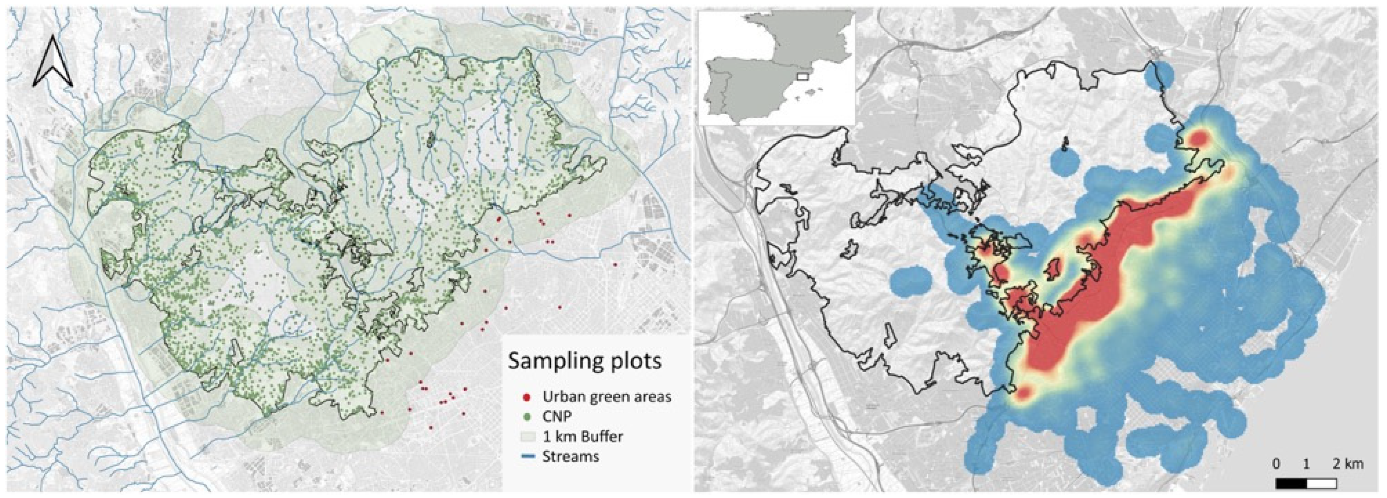
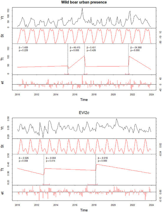
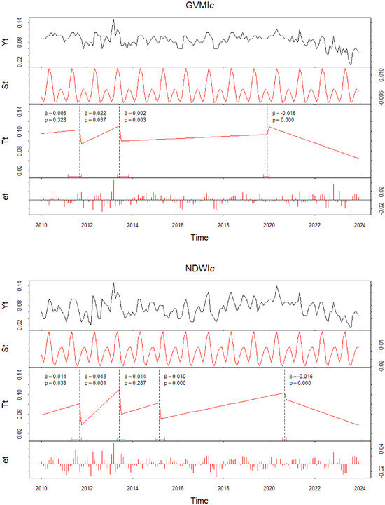
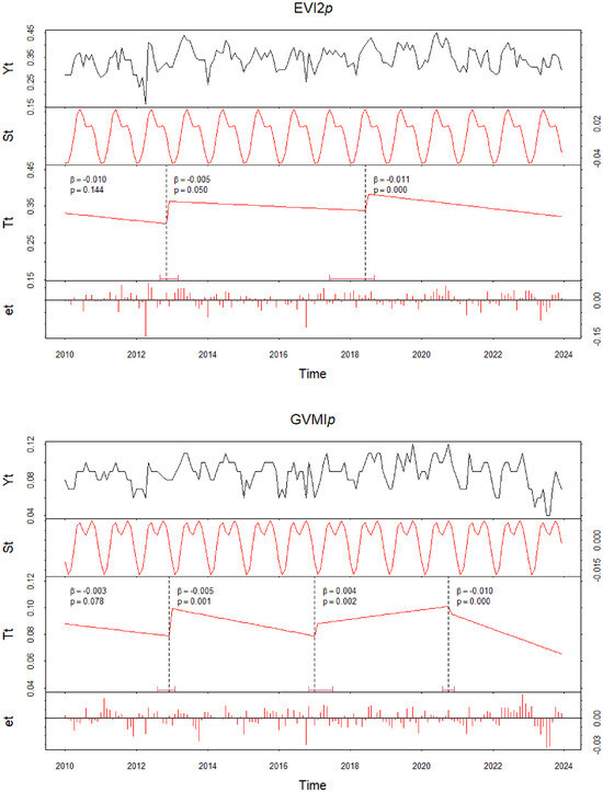
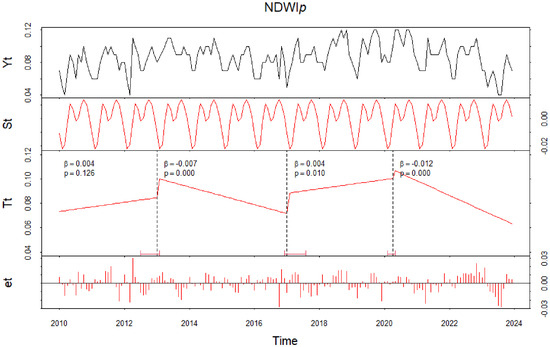
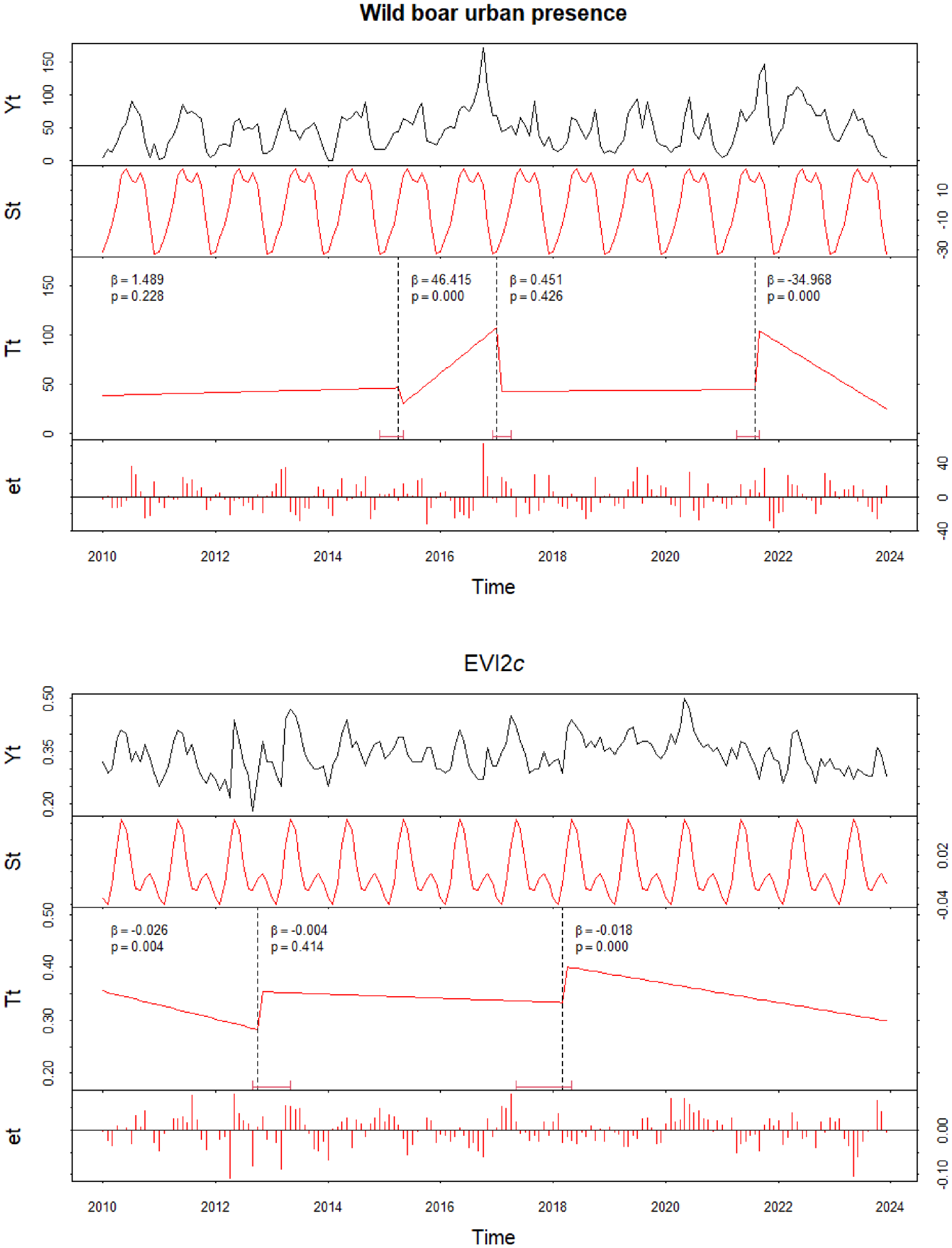
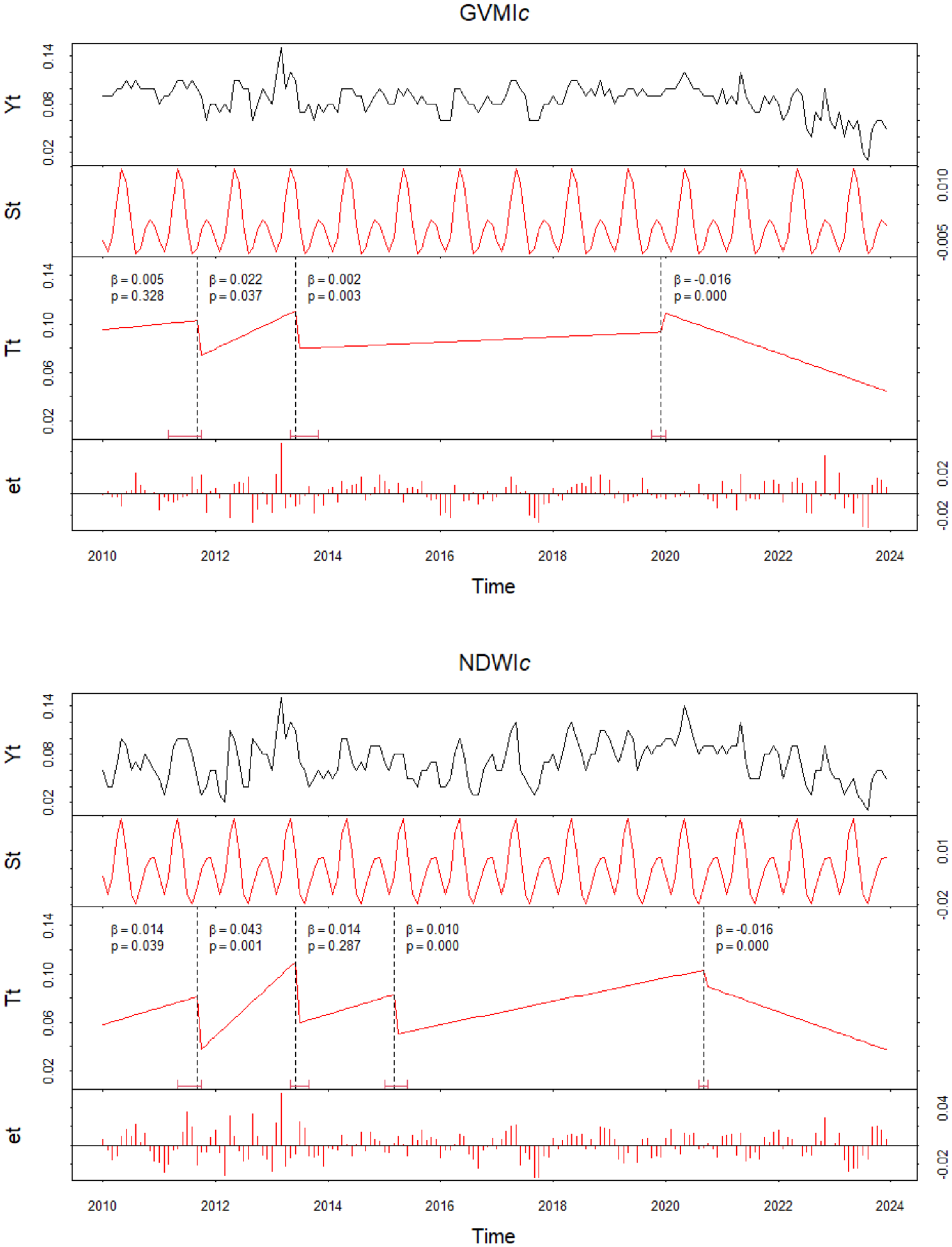
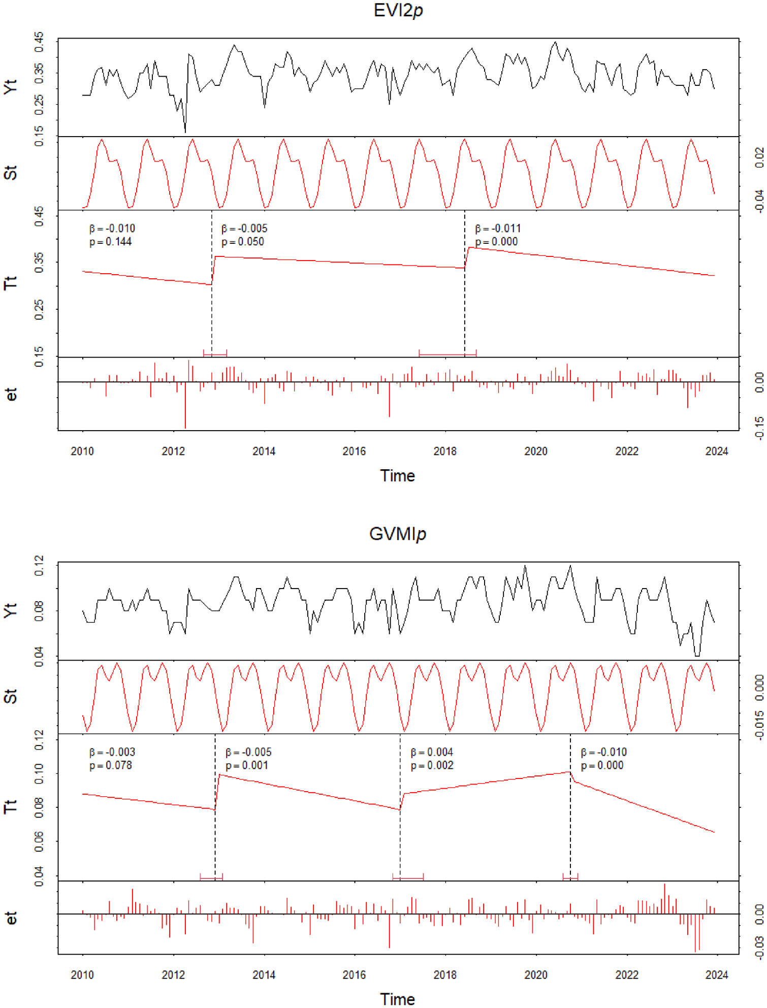
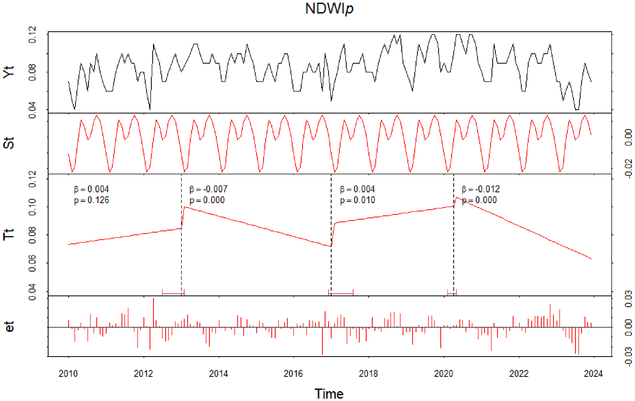
We obtained a decomposition of both TS, the original presences, and VI data into seasonal (St), trend (Tt), and remainder (et) components (Figure 2).
Figure 2.
Decomposition of TS (Yt) using the BFAST method for wild boar urban presence and the vegetation indices in the CNP (EVI2c, GVMIc and NDWIc) and urban green areas (EVI2p, GVMIp and NDWIp) between 2010 and 2023. BFAST separates each series into seasonal (St), trend (Tt), and remainder (et) components. Slope coefficients (β) and associated p-values are shown for each segmented trend.
The BFAST decomposition of wild boar urban presence in the urban green areas of Barcelona from 2010 to 2024 (Figure 2) identified a seasonal component (St) with consistent annual cycles and a distinct bimodal pattern, marked by peaks in spring and late summer and troughs in winter and midsummer. The long-term trend component (Tt) comprised four segments, each separated by statistically detected breakpoints (breakpoint dates in Table 1): an initial gradual, non-significant increase from 2010 to approximately April 2015 (β = 1.489, p = 0.228); a subsequent steep and highly significant rise between April 2015 and January 2017 (β = 46.415, p < 0.001), corresponding to the rapid escalation of incursions; a period of near-stabilisation or minimal increase from January 2017 to August 2021 (β = 0.451, p = 0.426); and a sharp, highly significant decline from August 2021 onwards (β = –34.968, p < 0.001), indicating a substantial reduction in urban presence.
Table 1.
Results from the BFAST trend component of urban wild boar presence and the vegetation indices of both urban green areas (EVI2p, GVMIp and NDWIp) and the CNP (EVI2c, GVMIc, and NDWIc).
For the CNP VI, we identified three breakpoints in the GVMI trend, two in the EVI2, and four in the NDWI (Table 1, Figure 2). On the other hand, for the urban green area VI, we identified two breakpoints in the EVI2 trend, and three in the GVMI and NDWI trends (Table 1, Figure 2). Table 1 presents the dates of abrupt changes, along with their magnitude and direction. It also includes the regression parameters of the piecewise model, depicting the values at the break date (intercept) and the recovery rate (slope).
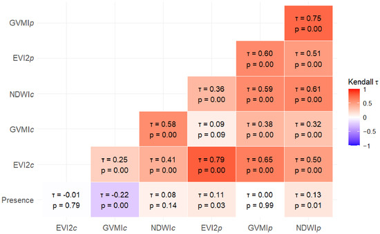
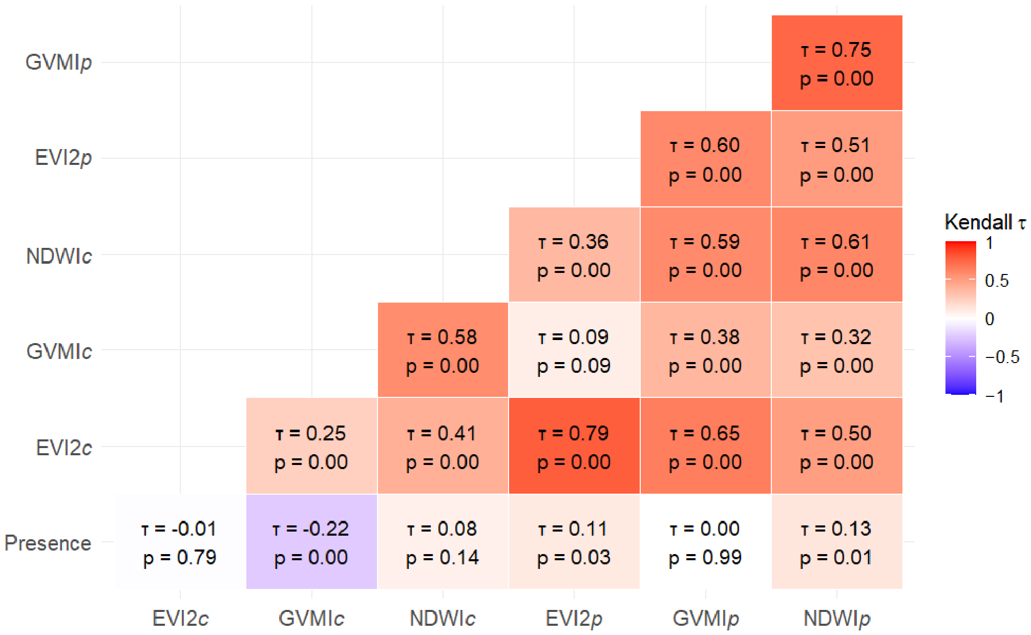
We detected significant correlations in the long-term trends of all vegetation indices for the urban green areas and the CNP, suggesting coherent long-term dynamics in vegetation greenness, moisture content, and water-related status (Figure 3). In contrast, the long-term trend in wild boar urban presence was only weak, largely non-significantly associated with the vegetation trend components. The strongest (albeit still weak) relationship was a significant negative correlation with vegetation moisture in the CNP (presence vs. GVMIc: τ = −0.22, p < 0.001). The presence of wild boar in urban areas was also weakly associated with long-term trends in urban green area EVI2 and NDWI (τ = 0.11, p = 0.03; and τ = 0.13, p = 0.01, respectively). However, none of these trends significantly predicted presence trends linearly (Table S1).
Figure 3.
Kendall correlation matrix of long-term trend components from BFAST for wild boar urban presence and RS-VIs from urban green areas (EVI2p, GVMIp, and NDWIp) and the CNP (EVI2c, GVMIc, and NDWIc). Colour intensity reflects correlation strength based on Kendall’s tau coefficient (τ): dark red indicates strong positive correlations, and dark blue, strong negative correlations. Statistical significance is based on p-values.
3.2. Relationship Among Seasonal Trends
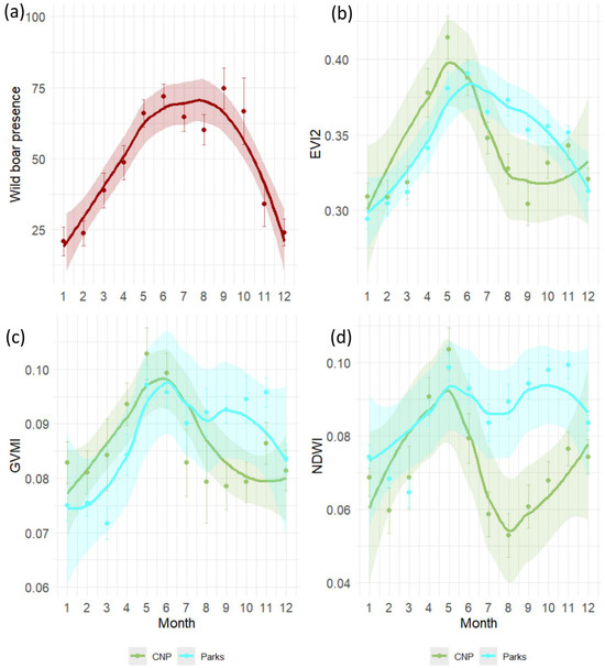
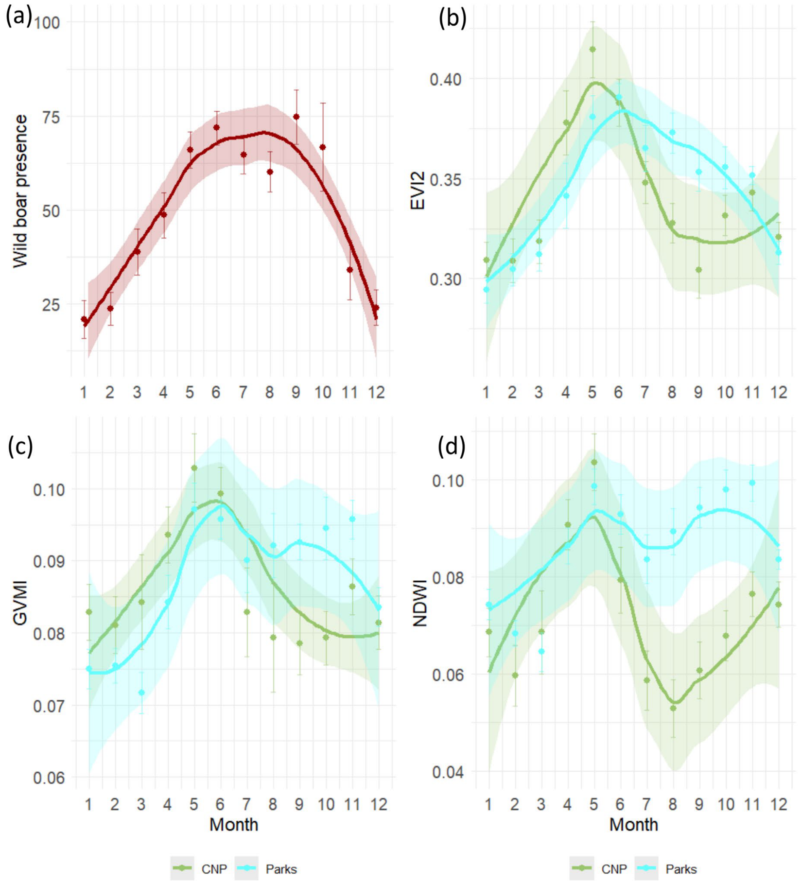
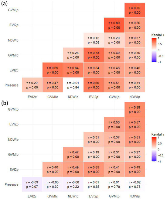
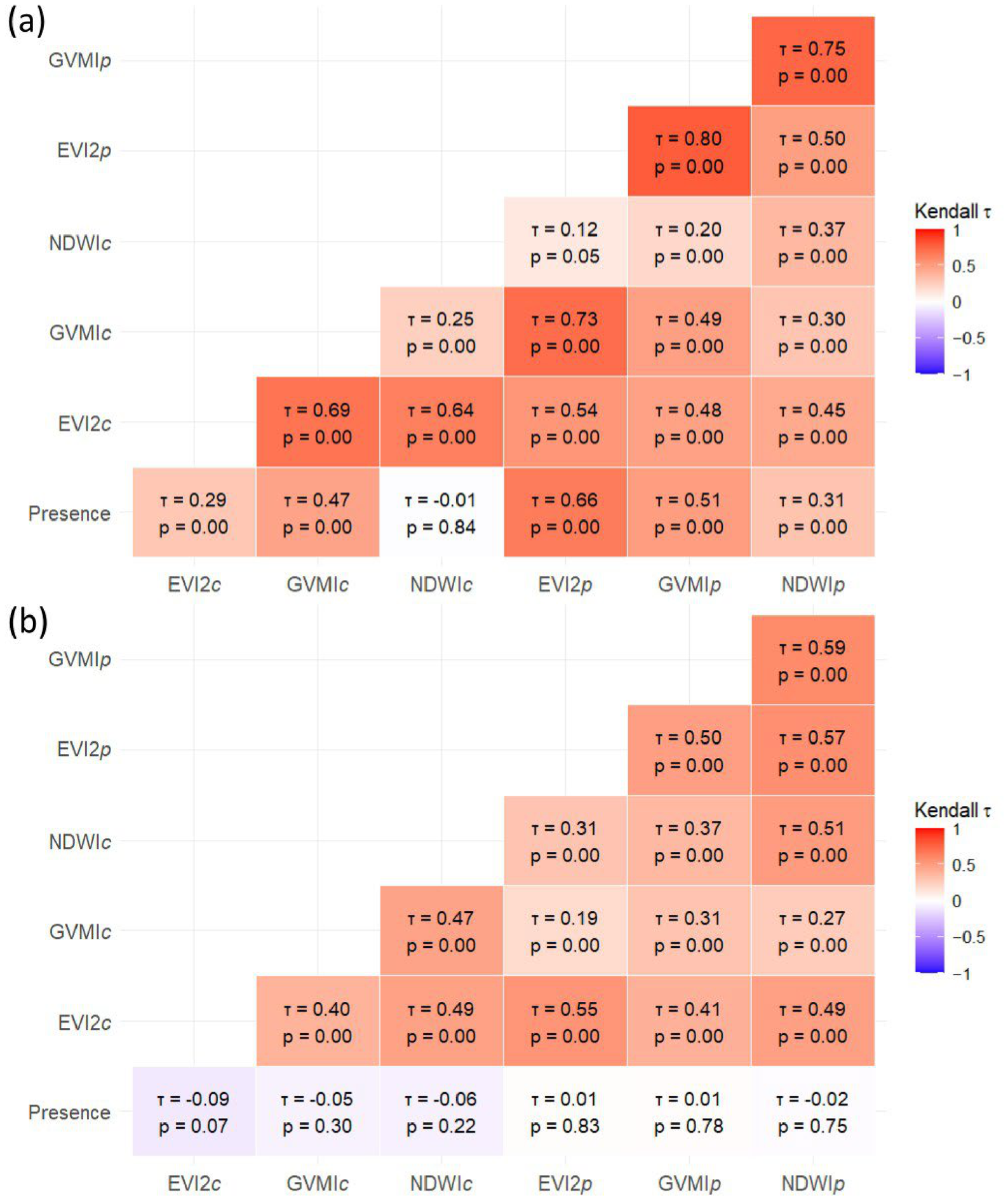
The GAMMs (Figure 4) revealed marked seasonal patterns in both the presence of wild boar in urban areas and all the RS-VIs. The results from the Kendall correlations between the standardised residuals and the predicted values of the models are represented in Figure 5. The specifications and goodness-of-fit of the GAMM models are presented in Table S2. On average, the models demonstrated moderate to good explanatory power, with a mean pseudo-R2 of 0.36. However, seasonal variation in VI differed among indices and habitats: seasonality explained a higher proportion of the variance of EVI2 and NDWI in both the urban green areas and CNP (pseudo-R2 ≈ 0.32–0.39; pseudo-R2 ≈ 0.40–0.43, respectively), whereas GVMI seasonality was stronger in the urban green areas (pseudo-R2 = 0.32) than in the CNP (pseudo-R2 = 0.14).
Figure 4.
Seasonal trends from generalised additive mixed models (GAMMs) for (a) wild boar urban presence and (b–d) vegetation indices (EVI2, GVMI, NDWI). Blue lines represent urban green areas and green lines represent the CNP. Solid lines with shaded bands represent the LOESS-smoothed model predictions (with 95% confidence intervals). Points and error bars show monthly means ± standard errors of the raw observed values, providing a direct view of the underlying data variability.
Figure 5.
Kendall correlation matrices between the (a) predicted values and (b) standardised residuals from the GAMMs. Subscript “p” indicates RS-VIs from urban green areas (EVI2p, GVMIp and NDWIp), whereas subscript “c” indicates RS-VIs from the CNP (EVI2c, GVMIc and NDWIc). Colour intensity reflects correlation strength based on Kendall’s tau coefficient (τ): dark red indicates strong positive correlations, and dark blue, strong negative correlations. Statistical significance is based on p-values.
The predicted values from the presence model were highly and positively associated with the urban green area EVI2 (τ = 0.66, p = 0.00) and moderately associated with the urban green area and CNP GVMI (τ = 0.51, p = 0.00; τ = 0.47, p = 0.00, respectively; Figure 5a). On the other hand, the standardised residuals of the presence model did not show significant correlations with any of the standardised residuals of the RS-VI GAMMs (Figure 5b).
Among all candidate GLMMs, the most parsimonious model with the lowest AICc value and the highest Akaike weight was the zero-inflated negative binomial model including GVMI for both habitats (Table 2). Both GVMI predictors (for the urban green areas and the CNP) were retained in the best model and were statistically significant (Table S3). The GVMI in the urban green areas was positively associated (β ≈ 24.1, p < 0.01) with urban wild boar presence, whereas the GVMI in the CNP was negatively associated (β ≈ −26.2, p < 0.05). The seasonal effects remained important, with a significant linear month term and a marginal quadratic effect, indicating non-linear seasonal variation in wild boar urban presence. The zero-inflation component was significant (p < 0.00), supporting the inclusion of a zero-inflated structure. The model achieved a high marginal R2 (~0.71) and conditional R2 (~0.93), indicating strong explanatory power after accounting for interannual variability.
Table 2.
Model selection and performance of candidate generalised linear mixed models (GLMMs) explaining wild boar urban presence.
3.3. Relationship Between Wild Boar Presence and Urban Green Area Features
The results from the PLSR model are shown in Table 3. Only the first latent component (t1) was significant (Q2 > 0.0975), explaining 22% of the variance in the log-transformed number of presences. The most influential predictors for constructing t1, based on their relative importance (derived from squared raw weights), were the log-transformed number of patches, total edge length, and the distance to the closest stream. These were also the variables with the highest loads and strongest correlations (logpatch: 0.88; logedge: 0.78; logdist_str: −0.61), evidencing their strong association with t1. On the other hand, the effect of the VIs and the remaining landscape metrics was negligible (Table 3). We also detected that the green areas located closer to streams had both higher mean presence and greater interannual variability in wild boar presence, whereas the green areas farther from these corridors consistently recorded fewer incursions (Figure S2).
Table 3.
Predictor weights of the partial least squares regression (PLSR) model explaining the number of wild boar presences within a 300-m buffer of the urban green areas located within a 1-km buffer of Collserola Natural Park (CNP).
4. Discussion
In this study, we explored whether remotely sensed vegetation indices (RS-VIs) and urban landscape characteristics could explain the temporal and spatial patterns of wild boar presence in an urban Mediterranean setting. The predictive value of the RS-VIs depended on the temporal scale analysed, being more informative at the annual scale.
4.1. Temporal Trends
The breakpoints in the VI temporal evolution at interannual scale could be expected, because most terrestrial biomes follow a non-linear trend related to greening and browning cycles [99]. The negative relationship between wild boar presence and GVMI in the CNP suggests that urban incursions were more frequent under drier environmental conditions. However, vegetation moisture alone did not explain the full temporal variability in urban presence. This indicates that RS-VIs primarily captured the broad seasonal conditions rather than the complete set of ecological processes driving urban incursions. Drought reduces soil moisture and forage availability, constraining rooting and promoting the use of anthropogenic food and water sources [24,43,44,100]. While vegetation dynamics provided a broad environmental seasonal context, they did not account for interannual and spatial variation in wild boar urban presence.
At the annual scale, the higher VI values in urban green areas than in the CNP during the scarcity period (Figure 4) correspond to a sharp decline under summer Mediterranean drought in the CNP [101], balanced by irrigation in the urban green areas [102]. The higher presence of wild boars in urban areas coinciding with the higher difference in VIs between the CNP and the urban green areas is probably explained by wild boar selecting moist soils for rooting during dry periods [24,43]. The association between urban presence and EVI2 in urban green areas further indicates that wild boars tracked vegetation productivity and greenness, likely reflecting increased availability of forage or cover [24].
Although GVMI emerged as the most informative RS-VI in the GLMMs, the seasonal GAMM fitted to GVMI in the CNP explained only a limited proportion of its temporal variability. This suggests that vegetation moisture does not follow a smooth seasonal pattern in the CNP but is influenced by short-term fluctuations such as rainfall pulses or soil heterogeneity [43,101]. Accordingly, the negative GVMIc effect detected in the GLMM should be interpreted as part of broader seasonal conditions rather than as a direct predictor of urban presence. The absence of correlations between model residuals further indicates that wild boar presence and vegetation indices vary similarly across seasons, but do not respond in parallel to short-term changes. Together, these results suggest that vegetation dynamics, as assessed by EVI2 and GVMI, represent a significant, but partial, driver of urban wild boar presence.
The seasonal increase in wild boar presence in urban areas when vegetation and moisture conditions in the CNP were still improving suggests that incursions are not driven solely by drought, but also by life-history processes [46,103,104]. In Mediterranean populations, farrowing occurs from late winter to spring, with lactation extending into early summer [105,106,107]. During this period, the energetic demands of wild boar females increase markedly due to milk production and the rapid growth of piglets [108,109]. These energetic constraints may promote exploratory movements and the exploitation of resource-rich anthropogenic environments, especially when natural forage is spatially limited or patchily distributed [37,44,46]. Under these conditions, irrigated urban green areas may temporarily provide higher profitable refuge and feeding opportunities than natural environments, even though the dry season is not completely established [24,44]. The subsequent decline in presence from late summer to autumn may reflect the end of lactation and improved natural foraging conditions associated with autumn rainfall and mast production [101], which likely draw individuals back toward natural habitats [39].
4.2. Urban Green Area Features
While seasonal dynamics explain when wild boars are more likely to enter the urban matrix, these processes do not determine how space is used within the city. Because PLSR analysis was based on a relatively small number of urban green areas, it should be interpreted as an exploratory summary of the main spatial gradients associated with wild boar presence rather than as a strong predictive model. Proximity to watercourses and landscape fragmentation have already been identified as key spatial predictors of wild boar occurrence in urban settings [24]. We refined these findings in two ways. First, by modelling aggregated presence within urban green areas, we captured variation in the intensity of habitat use rather than the occurrence probability alone. Second, by explicitly quantifying landscape configuration and integrating RS-VIs, we examined the main spatial gradients associated with habitat use. Similar to previous studies, our results suggest that natural corridors and landscape configuration are among the strongest landscape correlates of wild boar presence at the local scale. However, in contrast to the strong dominance of connectivity reported by Castillo-Contreras et al. [24], we detected a similar contribution of connectivity and fragmentation in explaining variation in wild boar presence across parks. Vegetation productivity and moisture within parks, however, had little influence on spatial patterns. This suggests that wild boar use of urban habitats is driven by the interaction between movement pathways and the spatial arrangement of resources and refuge, rather than by the primary production of urban vegetation patches [24,33,46].
The higher wild boar presence in the green areas closer to streams matches their role as natural corridors linking the CNP with the urban matrix [24]. This spatial pattern indicates that connectivity regulates the entry of individuals into the urban matrix, while neighbouring green spaces facilitate stepwise movement across the city [37,110]. The higher interannual variation in wild boar presence observed in highly connected urban green areas likely reflected fluctuations in the number of individuals entering the city, driven by changes in population size and dispersal [46]. Once within the city, local habitat structure may influence the intensity with which urban green areas are used [42]. Management interventions such as fencing or restricting anthropogenic food can reduce accessibility and habitat attractiveness [52], while human disturbance and lethal control have been shown to modify habitat selection through the creation of a “landscape of fear” [49,51,111,112,113]. Together, these processes may contribute to variation in urban habitat use through avoidance or displacement responses [37,45,114].
Wild boar urban presence was also higher in those urban green areas embedded in more heterogeneous landscapes (Figure S1). This is consistent with the hypothesis that these environments provide a closer juxtaposition of resources and refuge, factors previously associated with movement and habitat use in urban environments [24,33,115]. Such configurations can promote efficient foraging while maintaining access to cover, reducing movement costs and favouring repeated use [37,42]. This interpretation is consistent with previous findings showing increased displacement where resources are dispersed [45], but reduced home ranges where they are predictable and concentrated [27]. In contrast, wild boars tend to avoid less fragmented areas dominated by homogeneous urban land uses and densely built-up areas (Figure S1) [17]. The absence of fragmentation effects in studies using alternative metrics, such as “effective mesh size” [27,116], further suggests that its influence depends on how resources and risk are arranged within the urban matrix [24,33,46].
Several limitations should be considered when interpreting these patterns. First, pine and holm oak forests were excluded from the CNP vegetation analysis because evergreen Mediterranean forests show limited seasonal variation in NDVI- and EVI-type indices [66,67]. Consequently, the CNP RS-VI signal primarily reflects open and semi-open habitats and may not fully represent all habitats used by wild boar. Second, the CNP vegetation conditions were characterised using park-wide RS-VIs, which captured broad seasonal dynamics but not local variation near potential urban entry points. Future studies integrating spatially explicit vegetation metrics and animal movement data could clarify the influence of specific sectors of the CNP on urban incursions. Finally, anthropogenic food sources were not explicitly quantified [24,33,44], and the use of citizen-reported incidents may bias observations towards areas with greater human presence or conflict perception [28,29,33,117]. Behavioural adaptations such as increased nocturnality may further reduce detectability [44,118,119]. Nevertheless, the consistent effects of connectivity and landscape structure across parks suggest that the main spatial patterns identified are robust to these sources of uncertainty.
5. Conclusions
Wild boar presence in urban settings likely emerges from the interaction of processes operating at different scales: seasonal resource dynamics influence when incursions occur, and landscape connectivity and configuration constrain where animals access and use space within the urban landscape. RS-VIs captured Mediterranean vegetation dynamic differences between urban versus natural habitats, which influence the timing of urban presence. However, RS-VIs only partially represent these processes, limiting their predictive power. From a management perspective, our results highlight the importance of targeting highly connected areas that facilitate entry into the city. From a management perspective, our results suggest that parks near corridors may be suitable locations for pilot interventions aimed at reducing seasonal attractiveness, such as adjusting irrigation regimes or testing xerophytic plantings [52]. Our findings also highlight the need to further develop remote sensing approaches in urban systems, particularly through the integration of high-resolution movement data to better capture fine-scale habitat use.
Supplementary Materials
The following supporting information can be downloaded at: https://www.mdpi.com/article/10.3390/rs18132119/s1, Figure S1: Land cover composition within a 300 m buffer surrounding each selected urban green area; Figure S2: Conditional boxplots showing variation in wild boar urban presence across individual urban green areas located within 1 km of the CNP boundary; Table S1: Results from the linear regression of the long-term trends (BFAST trend component) of wild boar urban presence and vegetation indices of both urban green areas and the CNP, with Newey–West standard errors; Table S2: Summary of the generalised additive mixed models (GAMMs) fitted for seasonal patterns of vegetation indices and urban wild boar presence, including model specifications and pseudo-R2 as an indicator of goodness of fit; Table S3: Summary of the best generalised linear mixed model (GLMM); Table S4: Structural, compositional, and management characteristics of urban green areas included in this study.
Author Contributions
Conceptualisation, E.S., J.R.L.-O. and M.E.-G.; methodology, E.S., M.I.-Á., I.T.-B. and M.E.-G.; validation, J.R.L.-O., G.M., E.S. and M.I.-Á.; formal analysis, S.T., M.I.-Á. and M.E.-G.; resources, S.L. and J.R.L.-O.; data curation, A.C., S.T., M.I.-Á. and M.E.-G.; writing—original draft preparation, M.E.-G.; writing—review and editing, all co-authors; supervision, E.S.; project administration, S.L. and J.R.L.-O. All authors have read and agreed to the published version of the manuscript.
Funding
This work was developed within the framework of the contracts 13/051, 15/0174, 16/0243, and 18/0243-00PR-01 with the Ajuntament de Barcelona. This study benefited from the Research Grant PID2020-115046GB-I00 “Ecología, salud pública y gestión del jabalí urbano”, funded by the Spanish Ministerio de Ciencia e Innovación. María Escobar-González received support from the MICIU-UAB through an FPU grant (FPU19/04651).
Data Availability Statement
The datasets presented in this study are openly available in the CORA Repository (Universitat Autònoma de Barcelona) at: https://dataverse.csuc.cat/dataset.xhtml?persistentId=doi:10.34810/DATA3273 (accessed on 10 June 2026).
Acknowledgments
The authors thank the Ajuntament de Barcelona, especially Carme Maté, for providing access to the urban wild boar presence data collected by the local police service. During the preparation of this manuscript, the authors used ChatGPT (OpenAI, GPT-5.3) to generate R code for statistical analyses to assist with language refinement. The authors reviewed and edited all outputs and take full responsibility for the content of this publication.
Conflicts of Interest
The authors declare no conflicts of interest.
Abbreviations
The following abbreviations are used in this manuscript:
| CNP | Collserola Natural Park |
| EVI2 | Enhanced Vegetation Index 2 |
| GVMI | Global Vegetation Moisture Index |
| NDWI | Normalised Difference Water Index |
| RS-VI | Remotely Sensed Vegetation Indices |
| TS | Time Series |
References
- Goudie, A. The Human Impact on the Natural Environment, 4th ed.; MIT Press: Cambridge, MA, USA, 1994. [Google Scholar]
- Millennium Ecosystem Assessment. Ecosystems and Human Well-Being: Current State and Trends: Findings of the Condition and Trends Working Group; Biodiversity Synthesis; Island Press: Washington, DC, USA, 2005. [Google Scholar]
- World Urbanization Prospects. The 2018 Revision. Available online: https://www.un.org/development/desa/pd/sites/www.un.org.development.desa.pd/files/files/documents/2020/Jan/un_2018_wup_report.pdf (accessed on 15 March 2024).
- McKinney, M.L. Urbanization as a Major Cause of Biotic Homogenization. Biol. Conserv. 2006, 127, 247–260. [Google Scholar] [CrossRef]
- Kowarik, I. Novel Urban Ecosystems, Biodiversity, and Conservation. Environ. Pollut. 2011, 159, 1974–1983. [Google Scholar] [CrossRef] [PubMed]
- Aronson, M.F.J.; La Sorte, F.A.; Nilon, C.H.; Katti, M.; Goddard, M.A.; Lepczyk, C.A.; Warren, P.S.; Williams, N.S.G.; Cilliers, S.; Clarkson, B.; et al. A Global Analysis of the Impacts of Urbanization on Bird and Plant Diversity Reveals Key Anthropogenic Drivers. Proc. R. Soc. B Biol. Sci. 2014, 281, 20133330. [Google Scholar] [CrossRef] [PubMed]
- Johnson, M.T.J.; Munshi-South, J. Evolution of Life in Urban Environments. Science 2017, 358, eaam8327. [Google Scholar] [CrossRef] [PubMed]
- Bateman, P.W.; Fleming, P.A. Big City Life: Carnivores in Urban Environments. J. Zool. 2012, 287, 1–23. [Google Scholar] [CrossRef]
- Humphrey, J.E.; Haslem, A.; Bennett, A.F. Avoid, Adapt or Exploit: Re-Visiting Bird Responses to Urbanization Using a Novel Landscape Approach. Glob. Ecol. Conserv. 2023, 48, e02735. [Google Scholar] [CrossRef]
- DeStefano, S.; DeGraaf, R.M. Exploring the Ecology of Suburban Wildlife. Front. Ecol. Environ. 2003, 1, 95–101. [Google Scholar] [CrossRef]
- Ditchkoff, S.S.; Saalfeld, S.T.; Gibson, C.J. Animal Behavior in Urban Ecosystems: Modifications Due to Human-Induced Stress. Urban Ecosyst. 2006, 9, 5–12. [Google Scholar] [CrossRef]
- Soulsbury, C.D.; White, P.C.L. Human–Wildlife Interactions in Urban Areas: A Review of Conflicts, Benefits and Opportunities. Wildl. Res. 2016, 42, 541–553. [Google Scholar] [CrossRef]
- Kleemann, J.; Struve, B.; Spyra, M. Conflicts in Urban Peripheries in Europe. Land Use Policy 2023, 133, 106849. [Google Scholar] [CrossRef]
- Hosaka, T.; Numata, S. Spatiotemporal Dynamics of Urban Green Spaces and Human–Wildlife Conflicts in Tokyo. Sci. Rep. 2016, 6, 30911. [Google Scholar] [CrossRef] [PubMed]
- Licoppe, A.; Prévot, C.; Heymans, M.; Bovy, C.; Casaer, J.; Cahill, S. Wild Boar/Feral Pig in (Peri-)Urban Areas; International Union of Game Biologists: Brussels, Belgium, 2013. [Google Scholar]
- Castillo-Contreras, R.; Mentaberre, G.; Fernandez Aguilar, X.; Conejero, C.; Colom-Cadena, A.; Ráez-Bravo, A.; González-Crespo, C.; Espunyes, J.; Lavín, S.; López-Olvera, J.R. Wild Boar in the City: Phenotypic Responses to Urbanisation. Sci. Total Environ. 2021, 773, 145593. [Google Scholar] [CrossRef] [PubMed]
- Marin, C.; Couderchet, L.; Le Campion, G.; Werno, J. Wildlife and the City. Modelling Wild Boar Use of Urban Nature: Empirical Contribution, Methodological Proposal: Bordeaux (France) as an Example. Urban Ecosyst. 2024, 27, 1291–1312. [Google Scholar] [CrossRef]
- Rosell, C.; Carretero, M.A.; Bassols, E. Seguimiento de La Evolución Demográfica Del Jabalí (Sus scrofa) y Efectos Del Incremento de Presión Cinegética En El Parque Natural de La Zona Volcánica de La Garrotxa. Galemys Span. J. Mammal. 1998, 10, 59–74. [Google Scholar]
- Fonseca, C.; Da Silva, A.A.; Alves, J.; Vingada, J.; Soares, A.M.V.M. Reproductive Performance of Wild Boar Females in Portugal. Eur. J. Wildl. Res. 2011, 57, 363–371. [Google Scholar] [CrossRef]
- Massei, G.; Kindberg, J.; Licoppe, A.; Gačić, D.; Šprem, N.; Kamler, J.; Baubet, E.; Hohmann, U.; Monaco, A.; Ozoliņš, J.; et al. Wild Boar Populations up, Numbers of Hunters down? A Review of Trends and Implications for Europe. Pest Manag. Sci. 2015, 71, 492–500. [Google Scholar] [CrossRef] [PubMed]
- Vetter, S.G.; Puskas, Z.; Bieber, C.; Ruf, T. How Climate Change and Wildlife Management Affect Population Structure in Wild Boars. Sci. Rep. 2020, 10, 7298. [Google Scholar] [CrossRef] [PubMed]
- Carpio, A.J.; Apollonio, M.; Acevedo, P. Wild Ungulate Overabundance in Europe: Contexts, Causes, Monitoring and Management Recommendations. Mammal Rev. 2021, 51, 95–108. [Google Scholar] [CrossRef]
- Stillfried, M.; Fickel, J.; Börner, K.; Wittstatt, U.; Heddergott, M.; Ortmann, S.; Kramer-Schadt, S.; Frantz, A.C. Do Cities Represent Sources, Sinks or Isolated Islands for Urban Wild Boar Population Structure? J. Appl. Ecol. 2017, 54, 272–281. [Google Scholar] [CrossRef]
- Castillo-Contreras, R.; Carvalho, J.; Serrano, E.; Mentaberre, G.; Fernández-Aguilar, X.; Colom, A.; González-Crespo, C.; Lavín, S.; López-Olvera, J.R. Urban Wild Boars Prefer Fragmented Areas with Food Resources near Natural Corridors. Sci. Total Environ. 2018, 615, 282–288. [Google Scholar] [CrossRef] [PubMed]
- Sütő, D.; Heltai, M.; Katona, K. Quality and Use of Habitat Patches by Wild Boar (Sus scrofa) along an Urban Gradient. Biol. Futur. 2020, 71, 69–80. [Google Scholar] [CrossRef] [PubMed]
- Hagemann, J.; Conejero, C.; Stillfried, M.; Mentaberre, G.; Castillo-Contreras, R.; Fickel, J.; López-Olvera, J.R. Genetic Population Structure Defines Wild Boar as an Urban Exploiter Species in Barcelona, Spain. Sci. Total Environ. 2022, 833, 155126. [Google Scholar] [CrossRef] [PubMed]
- Marin, C.; Werno, J.; Le Campion, G.; Couderchet, L. Navigating Discreetly: Spatial Ecology of Urban Wild Boar in Bordeaux City’s Landscape of Fear, France. Sci. Total Environ. 2024, 954, 176436. [Google Scholar] [CrossRef] [PubMed]
- Conejero, C.; Castillo-Contreras, R.; González-Crespo, C.; Serrano, E.; Mentaberre, G.; Lavín, S.; López-Olvera, J.R. Past Experiences Drive Citizen Perception of Wild Boar in Urban Areas. Mamm. Biol. 2019, 96, 68–72. [Google Scholar] [CrossRef]
- Conejero, C.; González-Crespo, C.; Fatjó, J.; Castillo-Contreras, R.; Serrano, E.; Lavín, S.; Mentaberre, G.; López-Olvera, J.R. Between Conflict and Reciprocal Habituation: Human-Wild Boar Coexistence in Urban Areas. Sci. Total Environ. 2024, 936, 173258. [Google Scholar] [CrossRef] [PubMed]
- Ikeda, T.; Takahashi, H.; Igota, H.; Matsuura, Y.; Azumaya, M.; Yoshida, T.; Kaji, K. Effects of Culling Intensity on Diel and Seasonal Activity Patterns of Sika Deer (Cervus nippon). Sci. Rep. 2019, 9, 17205. [Google Scholar] [CrossRef] [PubMed]
- Ruiz-Fons, F. A Review of the Current Status of Relevant Zoonotic Pathogens in Wild Swine (Sus scrofa) Populations: Changes Modulating the Risk of Transmission to Humans. Transbound. Emerg. Dis. 2017, 64, 68–88. [Google Scholar] [CrossRef] [PubMed]
- Castillo-Contreras, R.; Marín, M.; López-Olvera, J.R.; Ayats, T.; Fernandez Aguilar, X.; Lavín, S.; Mentaberre, G.; Cerdà-Cuéllar, M. Zoonotic Campylobacter spp. and Salmonella spp. Carried by Wild Boars in a Metropolitan Area: Occurrence, Antimicrobial Susceptibility and Public Health Relevance. Sci. Total Environ. 2022, 822, 153444. [Google Scholar] [CrossRef] [PubMed]
- González-Crespo, C.; Martínez-López, B.; Conejero, C.; Castillo-Contreras, R.; Serrano, E.; López-Martín, J.M.; Lavín, S.; López-Olvera, J.R. Predicting Human-Wildlife Interaction in Urban Environments through Agent-Based Models. Landsc. Urban Plan. 2023, 240, 104878. [Google Scholar] [CrossRef]
- González-Crespo, C.; Martínez-López, B.; Conejero, C.; Castillo-Contreras, R.; Serrano, E.; López-Martín, J.M.; Lavín, S.; López-Olvera, J.R. Assessing the Epidemiological Risk at the Human-Wild Boar Interface through a One Health Approach Using an Agent-Based Model in Barcelona, Spain. One Health 2023, 17, 100598. [Google Scholar] [CrossRef] [PubMed]
- Mayer, J.J.; Garabedian, J.E.; Kilgo, J.C. Human Fatalities Resulting from Wild Pig Attacks Worldwide: 2000–2019. Hum.-Wildl. Interact. 2023, 17, 3–20. [Google Scholar] [CrossRef]
- McKee, S.C.; Psiropoulos, J.L.; Mayer, J.J. Frequency and Vehicle Damage Costs of Wild Pig-Vehicle Collisions in the United States, 2015–2022. Eur. J. Wildl. Res. 2024, 70, 44. [Google Scholar] [CrossRef]
- Stillfried, M.; Gras, P.; Börner, K.; Göritz, F.; Painer, J.; Röllig, K.; Wenzler, M.; Hofer, H.; Ortmann, S.; Kramer-Schadt, S. Secrets of Success in a Landscape of Fear: Urban Wild Boar Adjust Risk Perception and Tolerate Disturbance. Front. Ecol. Evol. 2017, 5, 157. [Google Scholar] [CrossRef]
- Csókás, A.; Schally, G.; Szabó, L.; Csányi, S.; Kovács, F.; Heltai, M. Space Use of Wild Boar (Sus scrofa) in Budapest: Are They Resident or Transient City Dwellers? Biol. Futur. 2020, 71, 39–51. [Google Scholar] [CrossRef] [PubMed]
- Stillfried, M.; Gras, P.; Busch, M.; Börner, K.; Kramer-Schadt, S.; Ortmann, S. Wild inside: Urban Wild Boar Select Natural, Not Anthropogenic Food Resources. PLoS ONE 2017, 12, e0175127. [Google Scholar] [CrossRef] [PubMed]
- Wevers, J.; Fattebert, J.; Casaer, J.; Artois, T.; Beenaerts, N. Trading Fear for Food in the Anthropocene: How Ungulates Cope with Human Disturbance in a Multi-Use, Suburban Ecosystem. Sci. Total Environ. 2020, 741, 140369. [Google Scholar] [CrossRef] [PubMed]
- Karami, P.; Tavakoli, S. Identification and Analysis of Areas Prone to Conflict with Wild Boar (Sus scrofa) in the Vineyards of Malayer County, Western Iran. Ecol. Model. 2022, 471, 110039. [Google Scholar] [CrossRef]
- Ciach, M.; Tetkowski, P.; Fedyń, I. Local-Scale Habitat Configuration Makes a Niche for Wildlife Encroaching into an Urban Landscape: Grubbing Sites of Wild Boar Sus scrofa in a City Matrix. Urban Ecosyst. 2023, 26, 629–639. [Google Scholar] [CrossRef]
- Cahill, S.; Llimona, F.; Gràcia, J. Spacing and Nocturnal Activity of Wild Boar Sus scrofa in a Mediterranean Metropolitan Park. Wildl. Biol. 2003, 9, 3–13. [Google Scholar] [CrossRef]
- Cahill, S.; Llimona, F.; Cabañeros, L.; Calomardo, F. Characteristics of Wild Boar (Sus scrofa) Habituation to Urban Areas in the Collserola Natural Park (Barcelona) and Comparison with Other Locations. Anim. Biodivers. Conserv. 2012, 35, 221–233. [Google Scholar] [CrossRef]
- Podgórski, T.; Baś, G.; Jędrzejewska, B.; Sönnichsen, L.; Śnieżko, S.; Jędrzejewski, W.; Okarma, H. Spatiotemporal Behavioral Plasticity of Wild Boar (Sus scrofa) under Contrasting Conditions of Human Pressure: Primeval Forest and Metropolitan Area. J. Mammal. 2013, 94, 109–119. [Google Scholar] [CrossRef]
- Toger, M.; Benenson, I.; Wang, Y.; Czamanski, D.; Malkinson, D. Pigs in Space: An Agent-Based Model of Wild Boar (Sus scrofa) Movement into Cities. Landsc. Urban Plan. 2018, 173, 70–80. [Google Scholar] [CrossRef]
- Llimona, F.; Cahill, S.; Tenés, A.; Camps, D.; Bonet-Arbolí, V.; Cabañeros, L. El Estudio de Los Mamíferos En Relación a La Gestión de Áreas Periurbanas. El Caso de La Región Metropolitana de Barcelona. Galemys Span. J. Mammal. 2007, 19, 215–234. [Google Scholar] [CrossRef]
- Barasona, J.; López-Olvera, J.; Beltrán-Beck, B.; Gortázar, C.; Vicente, J. Trap-Effectiveness and Response to Tiletamine-Zolazepam and Medetomidine Anaesthesia in Eurasian Wild Boar Captured with Cage and Corral Traps. BMC Vet. Res. 2013, 9, 107. [Google Scholar] [CrossRef] [PubMed]
- Torres-Blas, I.; Mentaberre, G.; Castillo-Contreras, R.; Fernández-Aguilar, X.; Conejero, C.; Valldeperes, M.; González-Crespo, C.; Colom-Cadena, A.; Lavín, S.; López-Olvera, J.R. Assessing Methods to Live-Capture Wild Boars (Sus scrofa) in Urban and Peri-Urban Environments. Vet. Rec. 2020, 187, e85. [Google Scholar] [CrossRef] [PubMed]
- Conejero, C.; López-Olvera, J.R.; González-Crespo, C.; Ráez-Bravo, A.; Castillo-Contreras, R.; Tampach, S.; Velarde, R.; Mentaberre, G. Assessing Mammal Trapping Standards in Wild Boar Drop-Net Capture. Sci. Rep. 2022, 12, 15090. [Google Scholar] [CrossRef] [PubMed]
- Escobar-González, M.; López-Martín, J.-M.; Mentaberre, G.; Valldeperes, M.; Estruch, J.; Tampach, S.; Castillo-Contreras, R.; Conejero, C.; Roldán, J.; Lavín, S.; et al. Evaluating Hunting and Capture Methods for Urban Wild Boar Population Management. Sci. Total Environ. 2024, 940, 173463. [Google Scholar] [CrossRef] [PubMed]
- González-Crespo, C.; Serrano, E.; Cahill, S.; Castillo-Contreras, R.; Cabañeros, L.; López-Martín, J.M.; Roldán, J.; Lavín, S.; López-Olvera, J.R. Stochastic Assessment of Management Strategies for a Mediterranean Peri-Urban Wild Boar Population. PLoS ONE 2018, 13, e0202289. [Google Scholar] [CrossRef] [PubMed]
- Ficetola, G.F.; Bonardi, A.; Mairota, P.; Leronni, V.; Padoa-Schioppa, E. Predicting Wild Boar Damages to Croplands in a Mosaic of Agricultural and Natural Areas. Curr. Zool. 2014, 60, 170–179. [Google Scholar] [CrossRef]
- Lee, O.; Schlichting, P.E.; Jo, Y.-S. Habitat Model for Wild Boar (Sus scrofa) in Bukhansan National Park, Seoul. J. Urban Ecol. 2022, 8, juac027. [Google Scholar] [CrossRef]
- Giefer, M.; An, L. Synthesizing Remote Sensing and Biophysical Measures to Evaluate Human–Wildlife Conflicts: The Case of Wild Boar Crop Raiding in Rural China. Remote Sens. 2020, 12, 618. [Google Scholar] [CrossRef]
- Pettorelli, N.; Laurance, W.F.; O’Brien, T.G.; Wegmann, M.; Nagendra, H.; Turner, W. Satellite Remote Sensing for Applied Ecologists: Opportunities and Challenges. J. Appl. Ecol. 2014, 51, 839–848. [Google Scholar] [CrossRef]
- Rouse, J.W.; Haas, R.H.; Schell, J.A.; Deering, D.W. Monitoring Vegetation Systems in the Great Plains with ERTS; NASA Special Publication; NASA: Washington, DC, USA, 1974; pp. 309–317.
- Gao, B. NDWI—A Normalized Difference Water Index for Remote Sensing of Vegetation Liquid Water from Space. Remote Sens. Environ. 1996, 58, 257–266. [Google Scholar] [CrossRef]
- Ceccato, P.; Gobron, N.; Flasse, S.; Pinty, B.; Tarantola, S. Designing a Spectral Index to Estimate Vegetation Water Content from Remote Sensing Data: Part 1. Remote Sens. Environ. 2002, 82, 188–197. [Google Scholar] [CrossRef]
- Ceccato, P.; Flasse, S.; Grégoire, J.-M. Designing a Spectral Index to Estimate Vegetation Water Content from Remote Sensing Data. Remote Sens. Environ. 2002, 82, 198–207. [Google Scholar] [CrossRef]
- Zarco-Tejada, P.J.; Rueda, C.A.; Ustin, S.L. Water Content Estimation in Vegetation with MODIS Reflectance Data and Model Inversion Methods. Remote Sens. Environ. 2003, 85, 109–124. [Google Scholar] [CrossRef]
- Turner, W.; Spector, S.; Gardiner, N.; Fladeland, M.; Sterling, E.; Steininger, M. Remote Sensing for Biodiversity Science and Conservation. Trends Ecol. Evol. 2003, 18, 306–314. [Google Scholar] [CrossRef]
- Velusamy, P.; Rajendran, S.; Mahendran, R.K.; Naseer, S.; Shafiq, M.; Choi, J.-G. Unmanned Aerial Vehicles (UAV) in Precision Agriculture: Applications and Challenges. Energies 2021, 15, 217. [Google Scholar] [CrossRef]
- Hàbitats—Benvinguts al Parc Natural de Collserola. Available online: https://parcnaturalcollserola.cat/habitats/ (accessed on 8 January 2024).
- Clima i Meteorologia—Benvinguts al Parc Natural de Collserola. Available online: https://parcnaturalcollserola.cat/clima-i-meteorologia/ (accessed on 7 January 2024).
- Lloret, F.; Lobo, A.; Estevan, H.; Maisongrande, P.; Vayreda, J.; Terradas, J. Woody Plant Richness and NDVI Response to Drought Events in Catalonian (Northeastern Spain) Forests. Ecology 2007, 88, 2270–2279. [Google Scholar] [CrossRef] [PubMed]
- Garbulsky, M.F.; Peñuelas, J.; Ogaya, R.; Filella, I. Leaf and Stand-Level Carbon Uptake of a Mediterranean Forest Estimated Using the Satellite-Derived Reflectance Indices EVI and PRI. Int. J. Remote Sens. 2013, 34, 1282–1296. [Google Scholar] [CrossRef]
- QGIS Development Team. QGIS Geographic Information System. 2019. Available online: https://www.scirp.org/reference/referencespapers?referenceid=2631129 (accessed on 16 January 2024).
- Gorelick, N.; Hancher, M.; Dixon, M.; Ilyushchenko, S.; Thau, D.; Moore, R. Google Earth Engine: Planetary-Scale Geospatial Analysis for Everyone. Remote Sens. Environ. 2017, 202, 18–27. [Google Scholar] [CrossRef]
- Earth Resources Observation and Science (EROS) Center. Landsat 8–9 Operational Land Imager/Thermal Infrared Sensor Level-2, Collection 2; Earth Resources Observation and Science (EROS) Center: Sioux Falls, SD, USA, 2013. [PubMed]
- Earth Resources Observation and Science (EROS) Center. Landsat 4–5 Thematic Mapper Level-2, Collection 2. 2020. Available online: https://data.usgs.gov/datacatalog/data/USGS:EROS5e83d1193824e4fc (accessed on 10 January 2024).
- Earth Resources Observation and Science (EROS) Center. Landsat 7 Enhanced Thematic Mapper Plus Level-2, Collection 2. 1999. Available online: https://data.usgs.gov/datacatalog/data/USGS:EROS5e83d12add5d4aa1 (accessed on 10 January 2024).
- R: A Language and Environment for Statistical Computing. 2024. Available online: https://www.scirp.org/reference/referencespapers?referenceid=3887298 (accessed on 16 November 2023).
- Hijmans, R. Terra. 2023. Available online: https://rhijmans.r-universe.dev/builds (accessed on 12 January 2024).
- Jiang, Z.; Huete, A.; Didan, K.; Miura, T. Development of a Two-Band Enhanced Vegetation Index Without a Blue Band. Remote Sens. Environ. 2008, 112, 3833–3845. [Google Scholar] [CrossRef]
- Index DataBase. Index: Global Vegetation Moisture Index. Available online: https://www.indexdatabase.de/db/i-single.php?id=372 (accessed on 26 April 2026).
- United States Geological Survey (USGS). NDVI: The Foundation of Remote Sensing Phenology. 2023. Available online: https://www.usgs.gov/special-topics/remote-sensing-phenology/science/ndvi-foundation-remote-sensing-phenology#overview (accessed on 28 May 2026).
- Shoshany, M. Satellite Remote Sensing of Natural Mediterranean Vegetation: A Review Within an Ecological Context. Prog. Phys. Geogr. Earth Environ. 2000, 24, 153–178. [Google Scholar] [CrossRef]
- Huete, A.; Didan, K.; Miura, T.; Rodriguez, E.P.; Gao, X.; Ferreira, L.G. Overview of the Radiometric and Biophysical Performance of the MODIS Vegetation Indices. Remote Sens. Environ. 2002, 83, 195–213. [Google Scholar] [CrossRef]
- Verbesselt, J.; Hyndman, R.; Newnham, G.; Culvenor, D. Detecting Trend and Seasonal Changes in Satellite Image Time Series. Remote Sens. Environ. 2010, 114, 106–115. [Google Scholar] [CrossRef]
- Cleveland, R.B.; Cleveland, W.S.; McRae, J.E.; Terpenning, I. STL: A Seasonal-Trend Decomposition Procedure Based on Loess. J. Off. Stat. 1990, 6, 3–73. [Google Scholar]
- Watts, L.M.; Laffan, S.W. Effectiveness of the BFAST Algorithm for Detecting Vegetation Response Patterns in a Semi-Arid Region. Remote Sens. Environ. 2014, 154, 234–245. [Google Scholar] [CrossRef]
- Newey, W.K.; West, K.D. A Simple, Positive Semi-Definite, Heteroskedasticity and Autocorrelation Consistent Covariance Matrix. Econometrica 1987, 55, 703. [Google Scholar] [CrossRef]
- Wood, S.N. Fast Stable Restricted Maximum Likelihood and Marginal Likelihood Estimation of Semiparametric Generalized Linear Models. J. R. Stat. Soc. Ser. B Stat. Methodol. 2011, 73, 3–36. [Google Scholar] [CrossRef]
- Wood, S.N. Generalized Additive Models: An Introduction with R, 2nd ed.; Chapman and Hall/CRC: New York, NY, USA, 2017. [Google Scholar]
- Wood, S.N.; Pya, N.; Säfken, B. Smoothing Parameter and Model Selection for General Smooth Models. J. Am. Stat. Assoc. 2016, 111, 1548–1563. [Google Scholar] [CrossRef]
- Zuur, A.F.; Ieno, E.N.; Elphick, C.S. A Protocol for Data Exploration to Avoid Common Statistical Problems. Methods Ecol. Evol. 2010, 1, 3–14. [Google Scholar] [CrossRef]
- Levene, H. Robust Tests for Equality of Variances. In Contributions to Probability and Statistics: Essays in Honor of Harold Hotelling; Stanford University Press: Palo Alto, CA, USA, 1960; Volume 2, pp. 278–292. [Google Scholar]
- Fasiolo, M.; Nedellec, R.; Goude, Y.; Wood, S.N. Scalable Visualisation Methods for Modern Generalized Additive Models. arXiv 2018, arXiv:1809.10632. [Google Scholar]
- Hartig, F. DHARMa. 2024. Available online: https://github.com/florianhartig/DHARMa (accessed on 16 December 2024).
- Brooks, M.E.; Kristensen, K.; van Benthem, K.J.; Magnusson, A.; Berg, C.W.; Nielsen, A.; Skaug, H.J.; Mächler, M.; Bolker, B.M. glmmTMB Balances Speed and Flexibility Among Packages for Zero-Inflated Generalized Linear Mixed Modeling. R J. 2017, 9, 378–400. [Google Scholar] [CrossRef]
- Nakagawa, S.; Schielzeth, H. A General and Simple Method for Obtaining R2 from Generalized Linear Mixed-effects Models. Methods Ecol. Evol. 2013, 4, 133–142. [Google Scholar] [CrossRef]
- Lüdecke, D. Ggeffects: Tidy Data Frames of Marginal Effects from Regression Models. J. Open Source Softw. 2018, 3, 772. [Google Scholar] [CrossRef]
- You, H. Quantifying Urban Fragmentation under Economic Transition in Shanghai City, China. Sustainability 2015, 8, 21. [Google Scholar] [CrossRef]
- Jung, M. LecoS. 2016. Available online: https://github.com/Martin-Jung/LecoS (accessed on 10 June 2026).
- Geladi, P.; Kowalski, B.R. Partial Least-Squares Regression: A Tutorial. Anal. Chim. Acta 1986, 185, 1–17. [Google Scholar] [CrossRef]
- Carrascal, L.M.; Galván, I.; Gordo, O. Partial Least Squares Regression as an Alternative to Current Regression Methods Used in Ecology. Oikos 2009, 118, 681–690. [Google Scholar] [CrossRef]
- Sanchez, G.; Trinchera, L.; Russolillo, G. plspm: Partial Least Squares Path Modeling (PLS-PM) 2009, 0.6.0. Available online: https://www.rdocumentation.org/packages/plspm/versions/0.6.0/topics/plspm (accessed on 10 January 2024).
- Ibañez-Álvarez, M.; Farràs Santasusana, P.; Calleja, J.A.; Rouco, C.; Brolly, M.; Burnside, N.G.; Baraza, E.; Bartolomé, J.; Serrano, E. Satellite-Based Monitoring of Primary Production in a Mediterranean Islet Post Black Rat Eradication. Remote Sens. 2021, 14, 101. [Google Scholar] [CrossRef]
- Calosi, M.; Gabbrielli, C.; Lazzeri, L.; Fattorini, N.; Cesaretti, G.; Burrini, L.; Petrillo, O.; Ferretti, F. Seasonal and Ecological Determinants of Wild Boar Rooting on Priority Protected Grasslands. Environ. Manag. 2024, 74, 268–281. [Google Scholar] [CrossRef] [PubMed]
- Blondel, J.; Aronson, J.; Bodiou, J.-Y.; Boeuf, G. (Eds.) The Mediterranean Region: Biological Diversity in Space and Time, 2nd ed.; Oxford biology; Oxford University Press: Oxford, UK; New York, NY, USA, 2010. [Google Scholar]
- Stutzer, D.C.; Lawrence, W.T.; Tucker, C.J.; Imhoff, M.L. The Use of Multisource Satellite and Geospatial Data to Study the Effect of Urbanization on Primary Productivity in the United States. IEEE Trans. Geosci. Remote Sens. 2000, 38, 2549–2556. [Google Scholar] [CrossRef]
- Gamelon, M.; Besnard, A.; Gaillard, J.-M.; Servanty, S.; Baubet, E.; Brandt, S.; Gimenez, O. High Hunting Pressure Selects for Earlier Birth Date: Wild Boar as a Case Study. Evolution 2011, 65, 3100–3112. [Google Scholar] [CrossRef] [PubMed]
- Servanty, S.; Gaillard, J.-M.; Ronchi, F.; Focardi, S.; Baubet, É.; Gimenez, O. Influence of Harvesting Pressure on Demographic Tactics: Implications for Wildlife Management: Harvesting & Demographic Tactics. J. Appl. Ecol. 2011, 48, 835–843. [Google Scholar] [CrossRef]
- Maillard, D.; Fournier, P. Timing and Synchrony of Births in the Wild Boar (Sus scrofa Linnaeus, 1758) in a Mediterranean Habitat: The Effect of Food Availability. Galemys Span. J. Mammal. 2004, 16, 67–74. [Google Scholar] [CrossRef]
- Santos, P.; Fernández-Llario, P.; Fonseca, C.; Monzón, A.; Bento, P.; Soares, A.M.V.M.; Mateos-Quesada, P.; Petrucci-Fonseca, F. Habitat and Reproductive Phenology of Wild Boar (Sus scrofa) in the Western Iberian Peninsula. Eur. J. Wildl. Res. 2006, 52, 207–212. [Google Scholar] [CrossRef]
- Podgórski, T.; Scandura, M.; Jędrzejewska, B. Next of Kin next Door—Philopatry and Socio-genetic Population Structure in Wild Boar. J. Zool. 2014, 294, 190–197. [Google Scholar] [CrossRef]
- Gittleman, J.L.; Thompson, S.D. Energy Allocation in Mammalian Reproduction. Am. Zool. 1988, 28, 863–875. [Google Scholar] [CrossRef]
- Ruf, T.; Vetter, S.G.; Painer, J.; Stalder, G.; Bieber, C. Atypical for Northern Ungulates, Energy Metabolism Is Lowest during Summer in Female Wild Boars (Sus scrofa). Sci. Rep. 2021, 11, 18310. [Google Scholar] [CrossRef] [PubMed]
- Crooks, K.R.; Sanjayan, M. (Eds.) Connectivity Conservation: Maintaining Connections for Nature. In Connectivity Conservation; Cambridge University Press: Cambridge, UK, 2006; pp. 1–20. [Google Scholar]
- Saïd, S.; Tolon, V.; Brandt, S.; Baubet, E. Sex Effect on Habitat Selection in Response to Hunting Disturbance: The Study of Wild Boar. Eur. J. Wildl. Res. 2012, 58, 107–115. [Google Scholar] [CrossRef]
- Drimaj, J.; Kamler, J.; Plhal, R.; Janata, P.; Adamec, Z.; Homolka, M. Intensive Hunting Pressure Changes Local Distribution of Wild Boar. Hum.-Wildl. Interact. 2021, 15, 22–31. [Google Scholar]
- Handschuh, M.; Linderoth, P.; Arnold, J.; Storch, I.; Bhardwaj, M. Anthropic Pressure Drives Resource Selection of an Adaptable Generalist in Human-dominated Landscapes. Conserv. Sci. Pract. 2024, 6, e13188. [Google Scholar] [CrossRef]
- Colomer, J.; Rosell, C.; Rodriguez-Teijeiro, J.D.; Massei, G. ‘Reserve Effect’: An Opportunity to Mitigate Human-Wild Boar Conflicts. Sci. Total Environ. 2021, 795, 148721. [Google Scholar] [CrossRef] [PubMed]
- Hidalgo-Toledo, S.P.; Pérez-González, J.; Hidalgo-de-Trucios, S.J. The Landscape of Fear and Wild Boar (Sus scrofa) Spatial Use in a Peri-Urban Area from West-Central Spain. Land 2025, 14, 1845. [Google Scholar] [CrossRef]
- Jaeger, J.A.G. Landscape Division, Splitting Index, and Effective Mesh Size: New Measures of Landscape Fragmentation. Landsc. Ecol. 2000, 15, 115–130. [Google Scholar] [CrossRef]
- Pop, M.I.; Gradinaru, S.R.; Popescu, V.D.; Haase, D.; Iojă, C.I. Emergency-line Calls as an Indicator to Assess Human–Wildlife Interaction in Urban Areas. Ecosphere 2023, 14, e4418. [Google Scholar] [CrossRef]
- Ohashi, H.; Saito, M.; Horie, R.; Tsunoda, H.; Noba, H.; Ishii, H.; Kuwabara, T.; Hiroshige, Y.; Koike, S.; Hoshino, Y.; et al. Differences in the Activity Pattern of the Wild Boar Sus scrofa Related to Human Disturbance. Eur. J. Wildl. Res. 2013, 59, 167–177. [Google Scholar] [CrossRef]
- Rosalino, L.M.; Teixeira, D.; Camarinha, C.; Pereira, G.; Magalhães, A.; Castro, G.; Lima, C.; Fonseca, C. Even Generalist and Resilient Species Are Affected by Anthropic Disturbance: Evidence from Wild Boar Activity Patterns in a Mediterranean Landscape. Mammal Res. 2022, 67, 317–325. [Google Scholar] [CrossRef]

Disclaimer/Publisher’s Note: The statements, opinions and data contained in all publications are solely those of the individual author(s) and contributor(s) and not of MDPI and/or the editor(s). MDPI and/or the editor(s) disclaim responsibility for any injury to people or property resulting from any ideas, methods, instructions or products referred to in the content. |
© 2026 by the authors. Licensee MDPI, Basel, Switzerland. This article is an open access article distributed under the terms and conditions of the Creative Commons Attribution (CC BY) license.