IRAS-SDLC: Lifecycle Risk Aggregation for Secure AI-Augmented Software Assurance Under RMF and Zero Trust

Abstract

Modern machine learning approaches for vulnerability detection achieve strong performance within specific datasets, yet their reliability degrades under domain shift, limiting their effectiveness for real-world secure software development lifecycle (SDLC) decision-making. In particular, probabilistic vulnerability predictions, while well-calibrated, exhibit instability across heterogeneous codebases, reducing their suitability as standalone risk indicators. This paper introduces Intelligent Risk-Adaptive Secure SDLC (IRAS-SDLC), a lifecycle risk aggregation framework for Secure AI-Augmented Software Assurance under the Risk Management Framework (RMF) and Zero Trust. The proposed framework integrates model-derived vulnerability likelihood with structured security metrics, specifically exploitability and impact derived from standardized Common Vulnerability Scoring System (CVSS) data, to construct a unified and interpretable risk representation. This formulation enables consistent prioritization across SDLC phases while aligning with RMF control families and Zero Trust continuous verification principles. By combining learned semantic signals with domain-independent security factors, IRAS mitigates the instability of vulnerability likelihood under distributional shifts and provides a more robust basis for cross-domain risk assessment. The framework embeds risk evaluation early in the SDLC, enabling proactive identification of vulnerabilities during the requirements and design phases rather than post-implementation detection. Empirical evaluation demonstrates that IRAS-SDLC maintains meaningful risk estimation under domain shift and significantly improves lifecycle outcomes. In particular, early risk identification yields negative detection latency relative to conventional methods and reduces simulated remediation costs by up to an order of magnitude. IRAS-SDLC bridges the gap between machine learning-based vulnerability prediction and governance-aligned security assurance by providing a stable, interpretable, and lifecycle-aware risk assessment mechanism that is directly compatible with RMF-based compliance workflows and Zero Trust architectures.

1. Introduction

Modern software systems face a persistent and escalating vulnerability crisis: the National Vulnerability Database (NVD) records sustained annual growth in reported Common Vulnerabilities and Exposures (CVEs), and application-layer weaknesses remain among the most exploited attack vectors across enterprise, cloud-native, and critical infrastructure systems [1,2]. Despite decades of research, the dominant industrial practice remains reactive vulnerabilities that are identified late in development, after design decisions have propagated through implementation, at a point where remediation is significantly more expensive and disruptive [3]. Addressing this structural gap requires integrating security reasoning earlier and more continuously across the SDLC.

The integration of software assurance into the SDLC has long been recognized as a critical strategy for reducing systemic vulnerabilities in complex information systems. Early work emphasized that security controls must be embedded throughout development rather than retrofitted during testing or deployment. Early work argued that executing security accreditation activities late in the lifecycle introduces avoidable risk and cost, advocating instead for security-driven requirements and design integration to reduce defect remediation overhead and improve overall system resilience [4]. Their framework, developed in the context of the Department of Defense (DoD) governance and the Defense Information Assurance Certification and Accreditation Process (DIACAP), anticipated what would later evolve into secure-by-design and DevSecOps paradigms.

Since 2010, however, the secure software landscape has undergone substantial transformation. DIACAP has been replaced by the Risk Management Framework (RMF), emphasizing continuous monitoring and risk-based authorization. Simultaneously, Zero Trust architectures [5,6,7,8] and DevSecOps pipelines have reshaped operational security expectations, requiring continuous assessment rather than periodic compliance validation [9,10,11]. These structural changes shift software assurance from a documentation-driven activity toward continuous, risk-adaptive engineering.

In parallel, advances in artificial intelligence (AI) have introduced new possibilities for predictive vulnerability detection and automated security reasoning. Machine learning techniques including transformer-based architectures and graph neural networks have demonstrated strong performance in identifying vulnerable code patterns and modeling exploit likelihood [12,13,14,15]. However, these models are almost exclusively evaluated at implementation time, in isolation from the broader lifecycle context, and without integration into governance-aligned risk frameworks. Moreover, empirical research has shown that early defect detection significantly reduces remediation cost compared to late-stage correction [3]. Despite these advances, few studies have systematically re-examined Secure SDLC integration under modern AI-augmented assurance capabilities and contemporary governance models.

This paper revisits Secure SDLC integration in the era of AI-augmented software assurance. We propose an Intelligent Risk-Adaptive Secure SDLC (IRAS-SDLC) framework that incorporates machine learning-based vulnerability prediction, graph-based dependency risk modeling, and continuous compliance validation aligned with RMF and Zero Trust principles. Through empirical evaluation and longitudinal vulnerability analysis (2010–2026), we assess whether AI-enabled early-stage detection substantively reduces remediation cost and detection latency compared to traditional late-stage security testing approaches.

Our contributions are threefold:

• We modernize the original Secure SDLC integration model by aligning it with RMF, Zero Trust, and DevSecOps architectures.
• We introduce an AI-augmented risk-adaptive framework for early vulnerability prediction across SDLC phases.
• We empirically evaluate early versus late vulnerability detection using publicly available vulnerability datasets spanning 2010–2026.

The remainder of this paper is organized as follows: Section 2 reviews the evolution of Secure SDLC from 2010 to 2026; Section 3 presents the IRAS-SDLC framework; Section 4 details the research methodology; Section 5 reports experimental results; Section 6 discusses findings and practical implications; Section 7 addresses limitations; Section 8 presents threats to validity; and Section 9 concludes the paper.

2. Evolution of Secure SDLC (2010–2026)

This section traces the key developments that have reshaped secure software development practice since 2010, spanning governance transitions, the rise of DevSecOps and Zero Trust, growing vulnerability complexity, and the emergence of AI-based assurance techniques. These trends collectively motivate the lifecycle-integrated, risk-adaptive framework proposed in this work.

2.1. Governance Transitions, DevSecOps, and Zero Trust

In 2010, Secure SDLC integration was aligned with the Defense Information Assurance Certification and Accreditation Process (DIACAP), which focused on documentation, control validation, and formal authorization before deployment [4]. Security assessment was often performed after development phases were completed, creating delays and increased remediation cost. DIACAP was later replaced by the Risk Management Framework (RMF), which introduced a lifecycle-based approach including categorization, control selection, implementation, assessment, authorization, and continuous monitoring [16,17]. Continuous Authorization to Operate has further emerged within defense environments [18], requiring security integration across all SDLC phases and continuous evidence generation rather than end-stage review.

DevOps introduced continuous integration and delivery pipelines [19], and security practices were subsequently embedded under DevSecOps [20,21]. DevSecOps promotes automated static analysis, dynamic testing, dependency scanning, and container security triggered at code commits and build processes, reducing the delay between defect introduction and detection [15]. However, most implementations still rely on rule-based tools rather than predictive systems [11], and continuous pipelines generate large volumes of security data that increasingly demand machine learning-based vulnerability prediction [22].

Zero Trust models assume that no user or system component is trusted by default, basing access decisions on continuous verification, device posture, identity, and risk scoring [6]. Zero Trust aligns with RMF continuous monitoring principles and requires software components to expose security-relevant telemetry supporting automated risk evaluation [23]. Together, these governance transitions indicate that modern Secure SDLC must support risk scoring at both design time and operational time through predictive and adaptive assurance models.

2.2. Growing Vulnerability Complexity and the Role of AI

Application-layer vulnerabilities have continued to increase in volume and complexity [1,2]. Vulnerability patterns are influenced by code complexity, churn rate, and developer activity [15], while modern systems incorporating open-source dependencies, third-party libraries, cloud-native microservices, and configuration-driven architectures further expand the attack surface [24,25]. Traditional static review methods struggle to scale with this complexity, supporting the need for automated and predictive security analysis.

Machine learning techniques have been applied to vulnerability detection, defect prediction, and exploit classification [12]. Graph neural networks improved performance by capturing structural program semantics [13], while transformer-based models such as CodeBERT advanced detection through pretrained code representations [14]. Subsequent work including LineVul [26] and VulBERTa [27] demonstrated improved localization accuracy and vulnerability classification. VulDetect further showed that pretrained language models can generalize across vulnerability categories without handcrafted feature engineering [28]. Graph-based approaches continue to model control flow and data flow dependencies [29], and hybrid models combining abstract syntax trees, control flow graphs, and token embeddings further enhance detection accuracy [13].

Large language models have more recently been explored for vulnerability detection and repair, with fine-tuned models achieving competitive performance alongside risks from insecure code generation [30,31]. AI-based systems have additionally been applied to fuzzing and anomaly detection [32], with learning-guided fuzzing improving coverage over random mutation strategies [33]. Despite this progress, most research evaluates models in isolation at the implementation phase. Limited work integrates AI systematically across all SDLC phases under governance models such as RMF and Zero Trust, motivating the IRAS-SDLC framework proposed in this work.

3. Intelligent Risk-Adaptive Secure SDLC Framework

Existing Secure SDLC models emphasize early integration of security controls within development workflows [4]. More recent research has advanced vulnerability detection using machine learning, deep learning, and language models [12,13,26,28], while DevSecOps studies focus on automated testing within CI/CD pipelines [20,21]. Governance frameworks such as RMF and Zero Trust promote continuous monitoring and risk-based authorization [6,17]. However, these streams of work are typically evaluated in isolation. Vulnerability prediction, compliance mapping, and runtime monitoring are rarely unified within a single lifecycle architecture. To address this gap, we propose the IRAS SDLC framework, which embeds AI models across SDLC phases, aggregates outputs through a quantitative risk engine, maps computed risk to RMF control families, and integrates continuous monitoring feedback to support adaptive assurance.

3.1. Design Principles

IRAS-SDLC embeds predictive modeling, quantitative risk scoring, and automated compliance validation across all SDLC phases. The framework is guided by five core principles summarized in Table 1.

Table 1. IRAS-SDLC design principles.

Principle	Description
Early Risk Estimation	Security embedded at requirements and design phases to reduce remediation cost [3,15].
Lifecycle-Wide AI Integration	AI models operate across all SDLC phases, beyond implementation-only evaluation [12,13,26].
Governance-Aligned Decision Support	Risk decisions aligned with RMF control structures rather than static rule enforcement [17].
Automated Compliance Validation	CI/CD pipelines generate machine-verifiable artifacts supporting continuous authorization [20,21].
Model Interpretability	Interpretable outputs support auditability and regulatory transparency [29].

3.2. Lifecycle Architecture Overview

IRAS-SDLC defines a layered architecture that integrates predictive analytics with governance enforcement. The first layer consists of SDLC phases including requirements, design, implementation, testing, deployment, and operations. The second layer embeds phase-specific AI components responsible for semantic analysis, structural modeling, and anomaly detection, producing phase-level security signals corresponding to vulnerability likelihood (V), exploitability (E), and impact (I). The third layer aggregates these signals within a unified risk engine that computes quantitative security scores using a lifecycle-aware formulation, enabling consistent risk propagation across SDLC phases. The fourth layer maps computed risk levels to RMF control families and generates compliance artifacts [17]. The fifth layer establishes runtime feedback loops between operational telemetry and development workflows, enabling continuous refinement of risk estimates and detection models consistent with Zero Trust principles [6].

3.3. AI Integration Across SDLC Phases

IRAS-SDLC integrates specialized AI components at each lifecycle phase. During requirements, natural language processing models analyze specifications to identify ambiguous or high-risk statements, leveraging transformer-based representations for semantic understanding [14]. During design, graph neural networks model dependency relationships and control flow structures to estimate attack surface exposure [13]. During implementation, pretrained language models and fine-tuned classifiers detect vulnerable patterns at commit time using contextual embeddings and structural program analysis [12,26,28]. During testing, learning-guided fuzzing and anomaly detection prioritize high-risk modules and improve vulnerability discovery rates [33]. During operations, telemetry-driven anomaly detection supports dynamic trust evaluation under Zero Trust continuous verification requirements [6].

3.4. Risk Scoring and Control Mapping Under RMF

IRAS-SDLC computes a quantitative risk score defined as

$$R=\alpha V+\beta E+\gamma I$$

(1)

where V denotes predicted vulnerability likelihood, E denotes exploitability probability, and I denotes impact aligned with RMF categorizations [17]. All components are normalized to the range $[0,1]$, ensuring comparability and bounded aggregation. The weighting coefficients satisfy $\alpha ,\beta ,\gamma \ge 0$ and $\alpha +\beta +\gamma =1$, enabling interpretable and convex risk estimation.

Vulnerability likelihood is derived from supervised classifiers trained on labeled datasets [12], exploitability is estimated using historical vulnerability data from NVD, including CVSS exploitability sub-scores [1], and impact reflects confidentiality, integrity, and availability requirements.

Computed risk scores are mapped to RMF control families through threshold-based risk tiers, enabling automated validation workflows and generation of machine-verifiable compliance artifacts.

Continuous Monitoring and Feedback Loops

IRAS-SDLC incorporates continuous monitoring consistent with RMF lifecycle guidance [17]. Runtime telemetry feeds anomaly detection systems that dynamically update risk components, including vulnerability likelihood V and exploitability E, based on observed system behavior and threat signals. These updates enable time-dependent refinement of the aggregated risk score R.

Updated risk metrics are propagated back into earlier SDLC phases, informing development prioritization, model retraining, and control adjustment. This feedback mechanism supports continuous recalibration of detection models and risk estimates, enabling adaptive trust evaluation aligned with Zero Trust continuous verification principles [6]. The complete IRAS-SDLC architecture is illustrated in Figure 1.

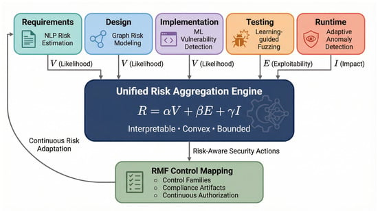
Figure 1. Intelligent Risk-Adaptive Secure SDLC architecture integrating phase-level AI analytics, a unified quantitative risk engine, RMF control mapping, and continuous feedback adaptation.

Table 2 summarizes how IRAS-SDLC differs from existing approaches across key capability dimensions, highlighting the unique combination of lifecycle-wide integration, quantitative risk aggregation, and governance alignment that distinguishes the proposed framework from prior work.

Table 2. Comparison of IRAS-SDLC against existing approaches across key capability dimensions. ✓ indicates capability present; × indicates capability absent.

Approach	Lifecycle-Wide	Risk Aggregation	RMF Aligned	Zero Trust	Explainability
Static Analysis	×	×	×	×	×
Graph-based ML (GCN/GAT)	×	×	×	×	×
Transformer-based ML (CodeBERT/LineVul)	×	×	×	×	✓
DevSecOps Pipelines	✓	×	×	×	×
IRAS-SDLC (Ours)	✓	✓	✓	✓	✓

3.5. Theoritical Risk Formulation

This subsection formalizes the mathematical foundation of the IRAS-SDLC risk aggregation model, defining the risk function, its theoretical properties, phase-indexed behavior, and decision mapping that underpin the empirical evaluation presented in Section 5.

3.5.1. Risk Variable Construction and Data Integration

The lifecycle risk formulation integrates model-derived vulnerability likelihood with standardized exploitability and impact metrics. Each component is constructed from the datasets and models introduced in previous sections.

The vulnerability likelihood is defined as

$$V=P(\mathrm{vulnerable}\mid x)$$

where V represents the predicted probability obtained from the fine-tuned CodeBERT model [14] evaluated on the Big-Vul dataset [34]. This value reflects the semantic likelihood that a given function contains a vulnerability.

Exploitability and impact are derived from the NVD using CVSS-based metrics [1]. Let E denote exploitability and I denote impact. Both quantities are normalized to the unit interval:

$$E,I\in [0,1]$$

Normalization is performed using min-max scaling over the observed range of CVSS exploitability and impact scores, ensuring compatibility with the probabilistic interpretation of V.

To align the datasets, vulnerability predictions from Big-Vul are associated with corresponding CVE entries where available, enabling the integration of model outputs with CVSS-derived metrics. This alignment provides a consistent representation of vulnerability likelihood, exploitability, and impact within a unified risk framework.

3.5.2. Linear IRAS Risk Formulation

The IRAS-SDLC framework defines a unified lifecycle risk score as a linear aggregation of vulnerability likelihood, exploitability, and impact. The risk function is formulated as

$$R=\alpha V+\beta E+\gamma I$$

subject to the constraint

$$\alpha +\beta +\gamma =1$$

where V represents the predicted vulnerability likelihood obtained from CodeBERT, E denotes normalized exploitability derived from CVSS metrics, and I denotes normalized impact. The coefficients $\alpha$, $\beta$, and $\gamma$ are weighting parameters that control the relative contribution of each component.

This formulation interprets risk as a multi-factor aggregation that integrates predictive, operational, and impact-driven signals into a single quantitative measure. The linear structure ensures interpretability, allowing each component to be directly associated with its contribution to the overall risk score. This is particularly important for governance-aligned decision-making, where transparency and traceability of risk factors are required.

Furthermore, the constraint $\alpha +\beta +\gamma =1$ ensures that the risk score remains normalized and comparable across different vulnerabilities and SDLC phases.

3.5.3. Theoretical Properties of Risk Aggregation

The linear risk aggregation model exhibits several desirable theoretical properties that support its use for lifecycle-aware security decision-making.

• Monotonicity: The risk function is monotonically increasing with respect to each component:

  $${\displaystyle \frac{\partial R}{\partial V}}=\alpha ,{\displaystyle \frac{\partial R}{\partial E}}=\beta ,{\displaystyle \frac{\partial R}{\partial I}}=\gamma$$
  Since $\alpha ,\beta ,\gamma >0$, an increase in vulnerability likelihood, exploitability, or impact results in a corresponding increase in the aggregated risk score. This ensures consistent prioritization of higher-risk components.
• Convexity: The risk function is linear in V, E, and I, and therefore convex over the domain ${[0,1]}^3$. This guarantees stable aggregation behavior and avoids nonlinear distortions in risk evaluation.
• Boundedness: Given that $V,E,I\in [0,1]$ and $\alpha +\beta +\gamma =1$, the aggregated risk score is bounded:

  $$0\le R\le 1$$
  This ensures that risk scores remain normalized and comparable across vulnerabilities and SDLC phases. These theoretical properties are summarized in Table 3.
  Table 3. Theoretical properties of the IRAS risk aggregation function, ensuring stable, interpretable, and comparable risk scores across vulnerabilities and SDLC phases.

  Property	Mathematical Condition	Implication
  Monotonicity	${\displaystyle \frac{\partial R}{\partial V}},{\displaystyle \frac{\partial R}{\partial E}},{\displaystyle \frac{\partial R}{\partial I}}>0$	Risk increases with vulnerability likelihood, exploitability, and impact, ensuring consistent prioritization
  Convexity	Linear in $V,E,I$	Guarantees stable aggregation behavior without introducing nonlinear distortions
  Boundedness	$0\le R\le 1$	Ensures normalized and comparable risk scores across vulnerabilities and SDLC phases

• Illustrative Example:

Consider a vulnerability instance with the following values:

$$V=0.80,E=0.60,I=0.70$$

and weights:

$$\alpha =0.5,\beta =0.3,\gamma =0.2$$

The aggregated risk score is computed as

$$R=\left(0.5\right)\left(0.80\right)+\left(0.3\right)\left(0.60\right)+\left(0.2\right)\left(0.70\right)=0.40+0.18+0.14=0.72$$

This example demonstrates the monotonic behavior of the risk function, where higher values of V, E, or I directly increase the overall risk score. The convex linear structure ensures that each component contributes proportionally according to its assigned weight, without introducing distortion. Furthermore, since all inputs lie within $[0,1]$ and the weights sum to one, the resulting risk score remains bounded, confirming that $R\in [0,1]$.

In practice, the weighting parameters $(\alpha ,\beta ,\gamma )$ can be determined based on organizational risk preferences and governance requirements. For example, security policies aligned with RMF or compliance frameworks may prioritize impact or exploitability, leading to higher values of $\beta$ or $\gamma$. Alternatively, weights can be dynamically tuned using historical incident data or optimization techniques to reflect an organization’s risk appetite and operational context.

3.5.4. Phase-Indexed Risk Modeling

To extend risk aggregation across the software development lifecycle, the IRAS-SDLC framework models risk as a function of the SDLC phase. Let $p\in \{1,2,3,4\}$ denote the phase index corresponding to requirements, design, implementation, and testing, respectively.

The phase-indexed risk score is defined as

$$R_p=\alpha V_p+\beta E_p+\gamma I_p$$

where $V_p$, $E_p$, and $I_p$ denote the vulnerability likelihood, exploitability, and impact estimated at phase p.

This formulation enables risk to be evaluated prior to implementation, allowing predictive signals to be incorporated earlier in the lifecycle. Let $t_i$ denote the phase at which a vulnerability is introduced and $t_d$ the phase at which it is detected. Detection latency is defined as

$$L=t_d-t_i$$

A reduction in $t_d$ corresponds to earlier detection, which directly influences remediation cost. Let ${\lambda }_p$ denote the cost escalation factor associated with phase p, with

$${\lambda }_1<{\lambda }_2<{\lambda }_3<{\lambda }_4$$

The expected remediation cost at phase p is given by

$$C_p={\lambda }_p{C}_b$$

where $C_b$ is the base remediation cost.

By enabling risk estimation at earlier phases ($p<3$), the IRAS-SDLC framework reduces detection latency and shifts remediation toward lower-cost phases. This establishes a direct relationship between phase-indexed risk modeling, detection timing, and cost efficiency, consistent with the lifecycle formulation presented in Section 4.3.

3.5.5. Phase Transition of Risk Across SDLC

To model how risk evolves across the software development lifecycle, the IRAS-SDLC framework represents risk as a phase-dependent quantity that is updated as new information becomes available.

The transition of risk between consecutive phases is defined as

$$R_{p+1}=R_p+{\Delta }_p$$

where ${\Delta }_p$ denotes the change in risk at phase p. Using the linear aggregation formulation, the update term can be expressed as

$${\Delta }_p=\alpha (V_{p+1}-V_p)+\beta (E_{p+1}-E_p)+\gamma (I_{p+1}-I_p)$$

This expression captures how changes in vulnerability likelihood, exploitability, and impact between phases contribute to the overall change in risk.

In practice, these updates arise from development and evaluation activities performed at each phase. For example, code commits and static analysis refine vulnerability likelihood during implementation, while dynamic testing and fuzzing further adjust risk estimates during validation. As a result, the components $V_p$, $E_p$, and $I_p$ are progressively updated, leading to corresponding changes in the aggregated risk score.

This formulation captures the fact that risk is not static, but evolves as the system progresses through SDLC phases. By incorporating phase-specific updates, IRAS-SDLC enables continuous refinement of risk estimates and supports more accurate prioritization decisions across the lifecycle.

3.5.6. Nonlinear Risk Extension

While the linear formulation provides an interpretable and stable aggregation mechanism, it assumes independence between vulnerability likelihood, exploitability, and impact. In practice, these factors often interact, leading to compounded risk effects that are not captured by linear combinations.

To model such interactions, the IRAS-SDLC framework extends the risk formulation with second-order terms:

$$R=\alpha V+\beta E+\gamma I+\delta (V·E)+\eta (V·I)$$

where $\delta$ and $\eta$ are interaction coefficients that capture the joint influence of vulnerability likelihood with exploitability and impact, respectively.

The interaction terms $V·E$ and $V·I$ model compound risk scenarios in which high vulnerability likelihood combined with high exploitability or high impact produces disproportionately higher risk. This reflects real-world conditions where easily exploitable or high-impact vulnerabilities require more urgent prioritization.

This nonlinear extension enhances the expressiveness of the risk model while preserving interpretability, enabling more accurate differentiation between moderate and critical vulnerabilities in lifecycle-aware decision-making.

4. Research Methodology

This section presents the datasets, experimental configuration, statistical validation framework, explainability analysis, and lifecycle-integrated evaluation metrics used to validate the proposed IRAS-SDLC framework. The objective is to rigorously evaluate early versus late vulnerability detection, lifecycle-integrated risk aggregation, governance-aligned compliance mapping, and statistically significant cost and latency reductions.

4.1. Datasets

Four publicly available datasets are used for empirical evaluation, covering real-world vulnerability records, synthetic benchmarks, and labeled open-source corpora. All datasets are preprocessed to ensure consistency in labeling, normalization of risk-related features, and alignment with SDLC phase encoding. Table 4 summarizes their characteristics and corresponding IRAS-SDLC components.

Table 4. Summary of datasets used for empirical evaluation.

Dataset	Type	Content	Purpose	Sample Size	IRAS Component
NVD (2010–2026) [1]	Real-world CVE records	CVE descriptions, CVSS metrics	Exploitability modeling	>200,000	Exploitability, Impact
Juliet Test Suite [35]	Synthetic benchmark	Weakness-labeled C/C++ and Java	Implementation-phase validation	92,980 programs	Controlled Validation
Devign [13]	Function-level dataset	Vulnerable and non-vulnerable graphs	Graph neural network evaluation	27,318 functions	Structural Risk
Big-Vul [34]	CVE-linked open-source	Vulnerable commits and labeled functions	Transformer-based detection	≈188,000 functions	Likelihood Estimation

4.2. Experimental Design

The experimental setup evaluates vulnerability detection across three lifecycle scenarios to compare early-stage prediction against implementation- and testing-phase identification.

• Early Detection Scenario: Risk estimation is performed during the requirements and design phases using NLP-based semantic analysis and graph-based architectural modeling. Vulnerability likelihood is predicted before source code implementation, allowing assessment of whether early analytical signals can reduce downstream defect propagation and remediation cost.
• Implementation Detection Scenario: Transformer-based and graph neural classifiers are applied during commit-time code evaluation. Vulnerability prediction is conducted at the function or module level, simulating secure coding practices integrated within a DevSecOps pipeline.
• Testing Detection Scenario: Learning-guided fuzzing and anomaly detection techniques are applied during dynamic testing. Vulnerabilities are identified through execution-based behavior analysis, representing traditional late-stage discovery mechanisms.

Predicted vulnerability likelihood values are integrated into the IRAS-SDLC risk formulation defined in Equation (1), enabling lifecycle-wide quantitative risk aggregation and governance-aligned control prioritization.

4.3. Lifecycle Modeling and Theoretical Cost Analysis

Detection latency and remediation cost are evaluated using a lifecycle-aware analytical model grounded in established software engineering cost escalation principles [3]. To formalize lifecycle-aware vulnerability detection, we model the SDLC as a discrete ordered set of phase indices:

$$p\in \{1,2,3,4\}$$

where phase $p=1$ corresponds to requirements engineering, $p=2$ to architectural and design activities, $p=3$ to implementation and coding, and $p=4$ to testing and validation. The ordering reflects increasing remediation complexity and escalation cost.

Let $t_i$ denote the phase at which a vulnerability is introduced into the system and $t_d$ denote the phase at which the vulnerability is detected. Detection latency is therefore defined as

$$L=t_d-t_i$$

A smaller value of L indicates earlier detection within the lifecycle and consequently lower expected remediation overhead.

4.3.1. Expected Detection Latency

Let $P(D=p)$ denote the probability that detection occurs at phase p. The expected latency is

$$\mathbb{E}\left[L\right]={\displaystyle \sum _{p=1}^4}P(D=p)(p-t_i)$$

Early detection reduces expected latency whenever

$${\displaystyle \sum _{p=1}^4}P(D=p)(p-t_i)<(4-t_i)$$

which holds whenever $P(D<4)>0$.

4.3.2. Remediation Cost Model

Let $C_b$ denote base remediation cost and ${\lambda }_p$ denote phase escalation multipliers:

$$C_p={\lambda }_p{C}_b$$

Expected remediation cost is

$$\mathbb{E}\left[C\right]={\displaystyle \sum _{p=1}^4}P(D=p){\lambda }_p{C}_b$$

IRAS-SDLC yields cost reduction when

$${\displaystyle \sum _{p=1}^4}P(D=p){\lambda }_p<{\lambda }_4$$

Given ${\lambda }_1<{\lambda }_2<{\lambda }_3<{\lambda }_4$, any non-zero early detection probability strictly reduces expected cost.

4.3.3. Phase Assignment Across Detection Methods

To enable lifecycle-based evaluation, each method is mapped to a representative SDLC detection phase based on its typical operational characteristics and deployment context. This abstraction allows for consistent comparison of detection latency across heterogeneous approaches. This mapping reflects typical deployment contexts reported in prior software security practices, where static analysis is applied post-implementation, machine learning operates at code-level evaluation, and IRAS-SDLC enables early-stage risk estimation. The phase assignments are summarized in Table 5.

• Static Analysis: Detection is primarily associated with later-stage validation, typically occurring during the testing phase or post-implementation analysis.
• ML-based Detection: Detection is performed during the implementation phase, where learned models analyze code artifacts after development.
• IRAS-SDLC: Detection is enabled during early lifecycle stages, particularly the requirements and design phases, through proactive risk estimation based on probabilistic modeling and integrated risk signals.

Table 5. Detection phase assignment across methods.

Method	Detection Phase
Static Analysis	Testing (Late-stage validation)
ML-based Detection	Implementation
IRAS-SDLC	Requirements/Design (Early-stage estimation)

Table 5. Detection phase assignment across methods.

Method	Detection Phase
Static Analysis	Testing (Late-stage validation)
ML-based Detection	Implementation
IRAS-SDLC	Requirements/Design (Early-stage estimation)

4.3.4. Detection Latency Modeling

Detection latency is defined as

$$L=t_d-t_i$$

where $t_i$ denotes the phase of vulnerability introduction and $t_d$ denotes the phase of detection. SDLC phases are encoded as ordinal values:

$$\mathrm{Requirements}=1,\mathrm{Design}=2,\mathrm{Implementation}=3,\mathrm{Testing}=4$$

For consistent comparison across methods, vulnerabilities are assumed to be introduced during the implementation phase ($t_i=3$), which represents a common point at which coding-related vulnerabilities emerge.

Under this assumption, latency is computed as follows:

• Static Analysis: $L=4-3=1$.
• ML-based Detection: $L=3-3=0$.
• IRAS-SDLC: $L=1-3=-2$.

A negative latency indicates that detection occurs prior to the assumed introduction phase, reflecting the ability of IRAS-SDLC to identify potential vulnerabilities early in the lifecycle through predictive risk estimation rather than post hoc analysis.

4.3.5. Remediation Cost Modeling

Remediation cost is modeled as

$$C_p={\lambda }_p{C}_b$$

where $C_b$ is a normalized base cost and ${\lambda }_p$ is a phase-dependent escalation factor reflecting the relative effort required to fix vulnerabilities at different stages of the SDLC.

The following scaling is used:

$${\lambda }_{\mathrm{Requirements}}=1,{\lambda }_{\mathrm{Design}}=2,{\lambda }_{\mathrm{Implementation}}=5,{\lambda }_{\mathrm{Testing}}=10$$

This scaling reflects the well-established principle that remediation costs increase significantly as development progresses, due to factors such as code dependencies, system integration complexity, and the need for re-testing and validation.

By combining this cost model with detection latency, earlier detection directly translates to lower remediation cost, enabling quantitative comparison of different detection strategies across the SDLC.

4.4. Lifecycle Risk Aggregation

Predicted vulnerability likelihood is denoted as

$$V=P(\mathrm{vulnerable}\mid x)$$

Exploitability E and impact I are derived from normalized CVSS metrics.

The unified lifecycle risk score is

$$R=\alpha V+\beta E+\gamma I$$

with $\alpha +\beta +\gamma =1$.

Risk stability is evaluated via variance:

$$\mathrm{Var}\left(R\right)={\displaystyle \frac{1}{n}}{\displaystyle \sum _{i=1}^n}{(R_i-\overline{R})}^2$$

4.5. Model Implementation

Transformer-based vulnerability detection is implemented using a fine-tuned CodeBERT model [14], a bidirectional transformer pretrained on source code and natural language pairs. CodeBERT is selected due to its demonstrated effectiveness in code representation learning and vulnerability classification tasks. The model is fine-tuned on the Big-Vul dataset for binary classification of vulnerable and non-vulnerable functions, while structural modeling on the Devign dataset is handled separately using graph neural network architectures. Source code is tokenized using the pretrained tokenizer, truncated or padded to fixed sequence length, and processed through the transformer encoder to obtain contextual embeddings. A linear classification head is applied to the pooled representation, enabling efficient adaptation of pretrained embeddings for binary vulnerability prediction while minimizing overfitting.

Graph-based structural features are incorporated using representations derived from abstract syntax trees and control flow graphs, following prior work [13].

For early-phase risk estimation, requirement statements are encoded using the same pretrained CodeBERT embedding layer to maintain representation consistency across lifecycle phases.

Training is performed using supervised learning with binary cross-entropy loss. For a predicted probability $\widehat{y}$ and ground-truth label $y\in \{0,1\}$, the loss function is defined as

$${\mathcal{L}}_{CE}=-\left[ylog\left(\widehat{y}\right)+(1-y)log(1-\widehat{y})\right]$$

For a dataset of size N, the average loss is

$$\mathcal{L}={\displaystyle \frac{1}{N}}{\displaystyle \sum _{i=1}^N}{\mathcal{L}}_{CE}^{\left(i\right)}$$

Optimization is performed using the Adam optimizer with weight decay regularization to improve generalization and training stability.

Data is partitioned into training (70%), validation (15%), and testing (15%) subsets using stratified sampling to preserve class balance. Hyperparameters including learning rate, batch size, and number of epochs are tuned via grid search on the validation set. All experiments are conducted under identical computational settings to ensure reproducibility. The key training hyperparameters used in our implementation are summarized in Table 6.

Table 6. Key hyperparameters for model training.

Hyperparameter	Value
Learning Rate	$2\times {10}^{-5}$ (typical fine-tuning)
Batch Size	16
Number of Epochs	3–5
Max Sequence Length	512
Optimizer	Adam
Weight Decay	0.01
Loss Function	Binary Cross-Entropy
Train/Validation/Test Split	70%/15%/15%

4.6. Model Explainability via SHAP

To support governance-aligned interpretability and auditability of AI-driven decisions, SHAP (SHapley Additive exPlanations) values are computed to quantify feature-level contributions to model predictions.

For a prediction function $f\left(x\right)$ defined over a feature set F, the SHAP value associated with feature i is given by

$${\varphi }_i=\sum _{S\subseteq F\setminus \left\{i\right\}}{\displaystyle \frac{\left|S\right|!\left(\right|F|-|S|-1)!}{\left|F\right|!}}\left[f(S\cup \{i\left\}\right)-f\left(S\right)\right]$$

where F denotes the complete set of input features and S represents any subset of features excluding feature i. The weighting term ensures a fair attribution based on Shapley value theory from cooperative game theory.

The quantity ${\varphi }_i$ represents the marginal contribution of feature i to the prediction outcome, averaged across all possible feature coalitions. Aggregated SHAP values are further analyzed to assess feature influence on vulnerability classification decisions and to examine their downstream impact on lifecycle risk scoring under the IRAS-SDLC framework.

4.7. Baseline Comparison

To isolate the contribution of lifecycle-wide integration and quantitative risk aggregation, the proposed IRAS-SDLC framework is compared against three representative baseline paradigms documented in prior research.

• Static Rule-Based Detection: This baseline represents traditional static analysis tools that rely on predefined vulnerability signatures and pattern-matching rules without predictive learning models. Such approaches are widely used in industrial static analysis systems and secure coding practices [36,37]. Security evaluation is typically confined to the implementation phase.
• Implementation-Only Machine Learning Detection: This configuration reflects learning-based vulnerability detection applied at the code level without lifecycle integration. Prior work has demonstrated transformer- and graph-based classifiers for function-level vulnerability prediction [12,13,26]. However, these models are generally evaluated solely during implementation and do not incorporate early-phase risk estimation or unified governance mapping.
• DevSecOps Without Risk Aggregation: This baseline models CI/CD-integrated security pipelines where static and dynamic testing are automated within deployment workflows [20,21]. While security checks are embedded into development cycles, these systems typically lack unified quantitative lifecycle risk scoring and structured RMF-aligned prioritization.

These baselines represent progressively increasing levels of automation and intelligence. The comparison enables assessment of whether lifecycle-wide AI integration and quantitative risk aggregation provide measurable improvements in detection accuracy, latency reduction, and remediation cost efficiency.

4.8. Statistical Validation Framework

To ensure robustness of results and assess both statistical significance and practical relevance, multiple complementary statistical validation techniques are employed.

4.8.1. ANOVA for Cost and Latency Comparison

Let ${\mu }_1$, ${\mu }_2$, and ${\mu }_3$ denote the mean remediation cost (or mean detection latency) under static detection, implementation-only machine learning, and IRAS-SDLC, respectively.

The null hypothesis is defined as

$$H_0:{\mu }_1={\mu }_2={\mu }_3$$

The ANOVA F-statistic is computed as

$$F={\displaystyle \frac{\text{Between-group variance}}{\text{Within-group variance}}}$$

Equivalently,

$$F={\displaystyle \frac{S{S}_B/(k-1)}{S{S}_W/(N-k)}}$$

where $S{S}_B$ denotes the between-group sum of squares, $S{S}_W$ denotes the within-group sum of squares, k is the number of groups, and N is the total number of observations.

Statistical significance is evaluated at the $\alpha =0.05$ level.

4.8.2. Survival Analysis for Detection Timing

Detection timing is modeled as a time-to-event process. Let T denote the SDLC phase at which a vulnerability is detected.

The Kaplan–Meier estimator of the survival function is defined as

$$\widehat{S}\left(t\right)=\prod _{t_i\le t}\left(1-{\displaystyle \frac{d_i}{n_i}}\right)$$

where $d_i$ denotes the number of detections at phase $t_i$, and $n_i$ denotes the number of samples at risk immediately prior to phase $t_i$.

To compare detection timing distributions across experimental conditions, the log-rank test statistic is computed as

$${\chi }^2={\displaystyle \frac{{(O-E)}^2}{V}}$$

where O represents the observed number of detections, E represents the expected number under the null hypothesis, and V denotes the variance of the difference. Statistical significance is evaluated at $\alpha =0.05$.

4.8.3. Confidence Intervals

To quantify estimation uncertainty, 95% confidence intervals are computed for all primary performance metrics, including F1-score, AUC, detection latency, and remediation cost.

For a sample mean $\overline{x}$ with standard deviation s and sample size n, the confidence interval is defined as

$$\overline{x}\pm z_{\alpha /2}{\displaystyle \frac{s}{\sqrt{n}}}$$

where $z_{\alpha /2}$ denotes the standard normal critical value (e.g., $1.96$ for 95% confidence). This provides an estimate of the variability and reliability of reported performance measures.

4.8.4. Effect Size (Cohen’s d)

To measure the magnitude of improvement between detection strategies, effect size is computed as

$$d={\displaystyle \frac{{\mu }_1-{\mu }_2}{s_p}}$$

where ${\mu }_1$ and ${\mu }_2$ are the mean values under two experimental conditions and $s_p$ is the pooled standard deviation defined as

$$s_p=\sqrt{{\displaystyle \frac{(n_1-1)s_1^2+(n_2-1)s_2^2}{n_1+n_2-2}}}$$

Effect size complements hypothesis testing by quantifying practical significance beyond statistical significance.

4.9. Evaluation Metrics

Model performance is evaluated using classification, timing, cost, and stability metrics. Let $TP$, $FP$, $TN$, and $FN$ denote true positives, false positives, true negatives, and false negatives, respectively.

• Precision

  $$\mathrm{Precision}={\displaystyle \frac{TP}{TP+FP}}$$
• Recall

  $$\mathrm{Recall}={\displaystyle \frac{TP}{TP+FN}}$$
• F1-score

  $$F1=2·{\displaystyle \frac{\mathrm{Precision}·\mathrm{Recall}}{\mathrm{Precision}+\mathrm{Recall}}}$$
• Receiver Operating Characteristic Area Under Curve (ROC-AUC).  
  The ROC curve plots the true positive rate (TPR) against the false positive rate (FPR) across varying decision thresholds. These are defined as

  $$\mathrm{TPR}={\displaystyle \frac{TP}{TP+FN}},\mathrm{FPR}={\displaystyle \frac{FP}{FP+TN}}$$
  The Area Under the ROC Curve (AUC) is computed as

  $$\mathrm{AUC}={\int }_0^1\mathrm{TPR}\left(\mathrm{FPR}\right)d\left(\mathrm{FPR}\right)$$
  AUC measures the probability that a randomly selected vulnerable sample is assigned a higher prediction score than a randomly selected non-vulnerable sample [38,39].
• Detection Latency  
  Detection latency quantifies the delay between vulnerability introduction and identification. Let $t_i$ denote the SDLC phase index at which a vulnerability is introduced, and $t_d$ denote the phase index at which it is detected. Latency is defined as

  $$\mathrm{Latency}=t_d-t_i$$
  Lower latency indicates earlier detection within the development lifecycle.
• Simulated Remediation Cost  
  Remediation cost is estimated using phase-dependent escalation multipliers derived from software engineering cost models [3]. Let $C_b$ denote base remediation cost and ${\lambda }_p$ denote the multiplier associated with SDLC phase p. The cost at phase p is

  $$C_p={\lambda }_p·C_b$$
• Risk Score Stability  
  Risk stability is measured as the variance of computed lifecycle risk scores:

  $$\mathrm{Var}\left(R\right)={\displaystyle \frac{1}{n}}{\displaystyle \sum _{i=1}^n}{(R_i-\overline{R})}^2$$

  where $R_i$ represents the risk score at phase i and $\overline{R}$ is the mean risk across phases.
  These metrics collectively evaluate classification accuracy, threshold robustness, detection timing, cost efficiency, governance alignment, and stability of lifecycle-integrated risk estimation under the IRAS-SDLC framework. The complete research methodology is illustrated in Figure 2.
  

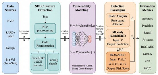  Figure 2. Research methodology illustrating dataset integration, SDLC phase-level analysis, agentic AI risk modeling, baseline comparison, and lifecycle-integrated evaluation using classification, latency, cost, and stability metrics.

5. Experimental Results

This section presents the empirical evaluation of the IRAS-SDLC framework across implementation-phase detection, structural modeling, lifecycle risk aggregation, latency and cost analysis, explainability, and statistical validation. Theoretical formulations underpinning these experiments are defined in Section 3 and Section 4.

5.1. Implementation-Phase Vulnerability Detection

This section evaluates vulnerability detection at the implementation phase using the Big-Vul dataset [34], a large-scale CVE-linked corpus of 188,636 function-level C/C++ samples. Three detection paradigms are assessed: static rule-based analysis, CodeBERT-based machine learning, and a simulated DevSecOps pipeline. The dataset is partitioned using stratified sampling (70/15/15) and performance is measured using accuracy, precision, recall, F1-score, and ROC-AUC, consistent with Section 4.9.

5.1.1. Static Rule-Based Detection

The static baseline represents traditional rule-based vulnerability detection approaches based on deterministic pattern matching. Let $\mathcal{R}=\{r_1,r_2,\dots ,r_m\}$ denote a predefined set of vulnerability rules, where each rule corresponds to a known unsafe pattern such as unsafe string operations, memory manipulation functions, or insecure API usage.

Given a source code sample x, the static detector applies each rule $r_j$ as a binary indicator function:  

$$r_j\left(x\right)=\left\{\begin{array}{cc}1,\hfill & \mathrm{if}\mathrm{pattern}{r}_j\mathrm{is}\mathrm{detected}\mathrm{in}x\hfill \\ 0,\hfill & \mathrm{otherwise}\hfill \end{array}\right.$$

The overall vulnerability prediction is defined as

$$\widehat{y}\left(x\right)=\left\{\begin{array}{cc}1,\hfill & \mathrm{if}{\sum }_{j=1}^m{r}_j\left(x\right)>0\hfill \\ 0,\hfill & \mathrm{otherwise}\hfill \end{array}\right.$$

Thus, a sample is classified as vulnerable if at least one rule is triggered. This corresponds to a logical OR aggregation over all predefined rules.

Unlike learning-based models, this approach does not estimate probabilities or optimize parameters, and therefore does not involve a training process or loss function. The detection capability is entirely dependent on the coverage and quality of the predefined rule set. For evaluation, the binary predictions $\widehat{y}\left(x\right)$ are compared against ground-truth labels $y\in \{0,1\}$ to compute standard classification metrics, including accuracy, precision, recall, F1-score, and ROC-AUC, as reported in Table 7.

Table 7. Static analysis performance on Big-Vul dataset.

Model	Accuracy	Precision	Recall	F1-Score	ROC-AUC	Loss
Static Analysis	0.81200	0.10828	0.26154	0.15315	0.55590	–

The static analysis baseline achieves an accuracy of 0.81200; however, this does not reflect strong detection capability. The precision of 0.10828 indicates a high false positive rate, while the recall of 0.26154 shows limited effectiveness in identifying vulnerable samples. The resulting F1-score of 0.15315 reflects poor overall performance. Furthermore, the ROC-AUC of 0.55590 suggests weak discriminative ability, only marginally better than random guessing. Since this approach does not involve model training, no loss value is reported. These results highlight the limitations of purely rule-based detection in capturing complex and context-dependent vulnerability patterns.

5.1.2. Implementation-Only Machine Learning Detection (CodeBERT)

The machine learning baseline is implemented using CodeBERT, a transformer-based model pretrained on source code. The model is fine-tuned for binary classification on the Big-Vul dataset, enabling it to learn contextual and semantic representations of code. Given an input source code sequence $x=(t_1,t_2,\dots ,t_n)$, where $t_i$ denotes a token, CodeBERT encodes the sequence using a transformer encoder to produce contextualized embeddings:

$$h=\mathrm{CodeBERT}\left(x\right)$$

A pooled representation $h_{\mathrm{pool}}$ is extracted from the final hidden states and passed through a linear classification layer:

$$z=w^{\top }{h}_{\mathrm{pool}}+b$$

The probability of vulnerability is then obtained using a sigmoid function:

$$\widehat{y}\left(x\right)=\sigma \left(z\right)={\displaystyle \frac{1}{1+e^{-z}}}$$

where $\widehat{y}\left(x\right)\in [0,1]$ represents the predicted vulnerability likelihood. A classification decision is made by applying a threshold $\tau$:

$$\widehat{y}\left(x\right)=\left\{\begin{array}{cc}1,\hfill & \mathrm{if}\sigma \left(z\right)\ge \tau \hfill \\ 0,\hfill & \mathrm{otherwise}\hfill \end{array}\right.$$

For evaluation, predicted labels are compared against ground-truth labels $y\in \{0,1\}$ to compute standard classification metrics, as reported in Table 8.

Table 8. Performance of the fine-tuned CodeBERT model on the Big-Vul test set. The classification threshold is selected to maximize F1-score.

Model	Accuracy	Precision	Recall	F1-Score	ROC-AUC	Loss
CodeBERT	0.97328	0.79837	0.71927	0.75676	0.96042	0.23061

The classification threshold is selected based on validation data to maximize the F1-score, rather than using a fixed threshold of 0.5. This ensures a balanced trade-off between precision and recall for vulnerability detection. CodeBERT achieves strong performance across evaluation metrics, with an F1-score of 0.75676, precision of 0.79837, and recall of 0.71927. The precision indicates effective control of false positives, while the recall demonstrates the model’s ability to identify a substantial proportion of vulnerable code instances. The overall accuracy of 0.97328 reflects strong classification performance, although it remains influenced by class imbalance in the dataset.

The ROC-AUC of 0.96042 indicates excellent discriminative capability, demonstrating that the model effectively ranks vulnerable and non-vulnerable samples across decision thresholds. The validation loss of 0.23061 confirms stable model convergence and reliable probabilistic outputs.

These results demonstrate that CodeBERT provides a strong implementation-phase detection baseline, capable of producing meaningful vulnerability likelihood estimates that can be integrated into the IRAS-SDLC framework.

5.1.3. DevSecOps Without Risk Aggregation

The DevSecOps baseline is simulated as a combined detection pipeline in which both static rule-based analysis and machine learning predictions are applied. A vulnerability is flagged if either method detects it, reflecting a typical CI/CD-integrated security workflow that emphasizes detection coverage without unified risk aggregation. Formally, let ${\widehat{y}}_s\left(x\right)$ denote the prediction from the static rule-based detector and ${\widehat{y}}_m\left(x\right)$ denote the prediction from the CodeBERT model. The DevSecOps decision rule is defined as

$$\widehat{y}\left(x\right)=\left\{\begin{array}{cc}1,\hfill & \mathrm{if}{\widehat{y}}_s\left(x\right)=1\vee {\widehat{y}}_m\left(x\right)=1\hfill \\ 0,\hfill & \mathrm{otherwise}\hfill \end{array}\right.$$

This corresponds to a logical OR aggregation of detection outputs, prioritizing vulnerability coverage over precision.

For evaluation, the combined predictions $\widehat{y}\left(x\right)$ are compared against ground-truth labels $y\in \{0,1\}$ to compute standard classification metrics, as reported in Table 9.

Table 9. DevSecOps baseline performance on Big-Vul dataset.

Model	Accuracy	Precision	Recall	F1-Score	ROC-AUC	Loss
DevSecOps (No Risk Aggregation)	0.84000	0.24868	0.72308	0.37008	0.78560	–

The DevSecOps configuration significantly improves recall to 0.72308, indicating that a larger proportion of vulnerabilities are detected compared to static analysis. However, this improvement comes at the cost of reduced precision, which drops to 0.24868 and results in a high false positive rate. The F1-score of 0.37008 reflects this imbalance between precision and recall.

The ROC-AUC of 0.78560 demonstrates moderate discriminative capability. In comparison, the CodeBERT model achieves stronger ranking performance with a ROC-AUC of 0.96042. This indicates that while the DevSecOps pipeline provides broader coverage, it lacks precise discrimination between vulnerable and non-vulnerable samples.

These results highlight the trade-off inherent in pipeline-based detection systems that prioritize coverage over precision. This limitation motivates the need for structured risk aggregation mechanisms such as IRAS-SDLC.

5.1.4. Baseline Comparison Results

Table 10 summarizes the performance of all three detection paradigms.

Table 10. Comparison of static analysis, DevSecOps, and CodeBERT on the Big-Vul dataset.

Model	Accuracy	Precision	Recall	F1-Score	ROC-AUC	Loss
Static Analysis	0.81200	0.10828	0.26154	0.15315	0.55590	–
DevSecOps (No Risk Aggregation)	0.84000	0.24868	0.72308	0.37008	0.78560	–
CodeBERT	0.97328	0.79837	0.71927	0.75676	0.96042	0.23061

Static analysis exhibits limited performance with near-random discriminative ability (ROC-AUC 0.56). DevSecOps improves recall significantly but at the cost of precision, reflecting a coverage-over-precision trade-off. CodeBERT achieves the strongest overall performance across all metrics, confirming the advantage of learning-based detection. These findings motivate the need for a unified risk aggregation framework integrating detection outputs with exploitability and impact metrics, as proposed in IRAS-SDLC and further illustrated in Figure 3.

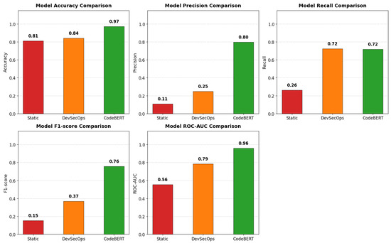
Figure 3. Performance comparison of static analysis, DevSecOps, and CodeBERT across accuracy, precision, recall, F1-score, and ROC-AUC. CodeBERT achieves the most balanced and consistently high performance, while DevSecOps improves recall at the expense of precision, and static analysis remains weak across all metrics.

5.2. Structural Vulnerability Modeling Using Graph Neural Networks

To evaluate the effectiveness of structural representations for vulnerability detection, we conduct experiments on the Devign dataset [13], which provides function-level labeled code samples designed for graph-based learning. Unlike token-based datasets such as Big-Vul [34], Devign captures program structure through implicit syntactic and semantic relationships, making it well-suited for graph neural network models.

In this setting, code samples are transformed into graph representations where nodes correspond to program tokens and edges encode sequential and structural relationships. Each graph is processed using graph neural network architectures to learn vulnerability patterns based on structural dependencies rather than purely sequential semantics.

5.2.1. Comparative Analysis of Graph Neural Architectures

Two graph neural network architectures are evaluated on the Devign dataset [13]. The Graph Convolutional Network (GCN) performs uniform neighborhood aggregation through message passing, capturing local structural dependencies within code graphs. The Graph Attention Network (GAT) extends this by introducing attention mechanisms that assign adaptive importance to neighboring nodes, enabling selective filtering of irrelevant structural signals. These differences in aggregation strategy lead to distinct trade-offs in detection performance, summarized in Table 11.

Table 11. Comparison of graph-based structural models on Devign dataset.

Model	Learning Mechanism	Accuracy	Precision	Recall	F1-Score	ROC-AUC
GCN	Neighborhood Aggregation	0.55900	0.55222	0.81190	0.65734	0.61358
GAT	Attention-Based Aggregation	0.58600	0.78919	0.28023	0.41360	0.70220

GCN achieves high recall through broad aggregation but at the cost of precision and discriminative power. GAT improves precision and ROC-AUC through attention-based weighting but reduces recall, reflecting a more conservative detection behavior. Both models remain constrained by limited semantic context, reinforcing the need for hybrid representations within the IRAS-SDLC framework.

5.2.2. Representation-Level Comparison

Table 12 compares graph-based models with token-based and rule-based approaches across different input representations and learning mechanisms.

Table 12. Comparison across representation paradigms.

Model	Accuracy	Precision	Recall	F1-Score	ROC-AUC	Input	Learning & Strength
Static Analysis	0.81200	0.10828	0.26154	0.15315	0.55590	Patterns	Rule-based; deterministic detection
DevSecOps Pipeline	0.84000	0.24868	0.72308	0.37008	0.78560	Hybrid	Pipeline integration; high recall
GCN	0.55900	0.55222	0.81190	0.65734	0.61358	Graph	Structural learning; high coverage
GAT	0.58600	0.78919	0.28023	0.41360	0.70220	Graph	Attention-based; high precision
CodeBERT	0.97328	0.79837	0.71927	0.75676	0.96042	Tokens	Semantic learning; contextual understanding

The results reveal clear trade-offs across representation paradigms. Static analysis exhibits near-random discriminative ability (ROC-AUC 0.56) and low precision, reflecting the limitations of rule-based detection in capturing complex vulnerability patterns. The DevSecOps pipeline improves recall significantly (0.72) through combined detection coverage but suffers from reduced precision (0.25) and moderate ROC-AUC (0.79), exposing the limitations of loosely integrated workflows without unified risk scoring.

Among graph-based models, GCN achieves the highest recall (0.81) through broad neighborhood aggregation, capturing a large proportion of vulnerable instances at the cost of precision. GAT improves precision (0.79) and ROC-AUC (0.70) through attention-based weighting but reduces recall substantially (0.28), reflecting a precision-coverage trade-off inherent to structural approaches. Both graph models remain constrained by limited semantic context.

CodeBERT achieves the strongest overall performance, with the highest accuracy (0.97), precision (0.80), F1-score (0.76), and ROC-AUC (0.96), confirming that deep semantic representations provide superior discrimination between vulnerable and non-vulnerable samples. These results are further illustrated in Figure 4.

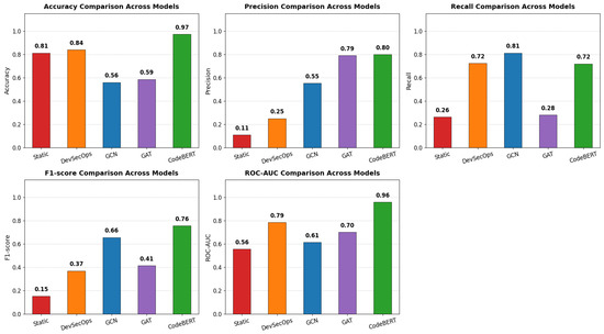
Figure 4. Performance comparison across static analysis, DevSecOps, GCN, GAT, and CodeBERT models using accuracy, precision, recall, F1-score, and ROC-AUC.

Collectively, these findings reinforce the need for a unified framework integrating semantic, structural, and lifecycle-level signals. The strong discriminative performance of CodeBERT ensures that the predicted vulnerability likelihood $V=P(\mathrm{vulnerable}\mid x)$ provides a reliable probabilistic foundation for subsequent lifecycle risk aggregation in IRAS-SDLC.

5.3. Lifecycle Risk Aggregation Under IRAS-SDLC

The results in Section 5.1 and Section 5.2 demonstrate that semantic and structural models provide strong but partial perspectives on vulnerability detection. However, these approaches remain focused on implementation-phase detection and do not directly support lifecycle-aware prioritization or governance-aligned decision-making. To address this, IRAS-SDLC introduces a unified lifecycle risk aggregation mechanism combining model-based vulnerability likelihood with exploitability and impact metrics derived from the NVD [1], utilizing CVE records spanning 2010–2026 with CVSS sub-scores normalized to $[0,1]$ for integration into Equation (1), consistent with the theoretical framework defined in Section 4.3 and Section 4.4.

5.3.1. Risk-to-Decision Mapping

To translate quantitative risk scores into actionable security decisions, the IRAS-SDLC framework defines a mapping between risk levels, remediation actions, and governance-aligned control responses. This mapping enables consistent prioritization of vulnerabilities across SDLC phases. The risk-to-decision mapping is presented in Table 13.

Table 13. Risk-to-decision mapping under IRAS-SDLC.

Risk Range	Risk Level	Action	Governance Interpretation
$0.0\le R<0.4$	Low	Monitor	Continuous monitoring with no immediate remediation required; aligns with low-impact RMF controls
$0.4\le R<0.7$	Medium	Patch/Mitigate	Trigger control enforcement and remediation planning; corresponds to moderate-risk RMF categorization
$0.7\le R\le 1.0$	High	Immediate Fix	Priority mitigation and rapid response required; aligned with high-impact RMF controls and security escalation

5.3.2. Empirical Risk Aggregation Results

This section presents the empirical evaluation of the IRAS-SDLC framework by integrating calibrated vulnerability likelihood, exploitability, and impact into a unified lifecycle risk score. The objective is to demonstrate how probabilistic model outputs can be transformed into structured, interpretable, and decision-supportive risk representations across the software development lifecycle.

Probabilistic Modeling of Vulnerability Likelihood

The vulnerability likelihood is defined as a calibrated probability:

$$V=P(y=1\mid x)$$

where the probability is obtained from the softmax output of a fine-tuned CodeBERT model and further calibrated using temperature scaling. To ensure probabilistic reliability, the model was evaluated using the Brier Score and Expected Calibration Error (ECE). The model achieved a Brier Score of 0.0638 and an ECE of 0.0483, indicating strong alignment between predicted confidence and observed outcomes. The resulting probability distribution spans a wide range from approximately 0.02 to 0.99, confirming that the model produces meaningful and well-calibrated confidence estimates suitable for downstream risk aggregation.

The distribution and calibration characteristics of the predicted vulnerability probabilities are illustrated in Figure 5, providing further validation of the probabilistic modeling.

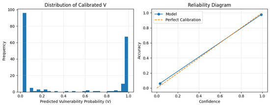
Figure 5. Distribution and calibration of predicted vulnerability probabilities. The left plot shows the distribution of calibrated probabilities, highlighting confident separation between low and high-risk instances. The right plot presents the reliability diagram, demonstrating strong alignment between predicted confidence and empirical accuracy.

• Risk Aggregation Variables: The IRAS formulation combines three complementary components, as summarized in Table 14. Vulnerability likelihood (V) represents a calibrated probabilistic estimate derived from CodeBERT, while exploitability (E) and impact (I) are obtained from normalized CVSS metrics from the NVD [1]. The weighting scheme $(\alpha ,\beta ,\gamma )=(0.5,0.3,0.2)$ balances learned semantic signals with standardized severity indicators, enabling a principled transition from prediction to risk-aware decision variables.
  Table 14. IRAS variables and weights.

  Variable	Symbol	Weight	Description
  Vulnerability Likelihood	V	$\alpha =0.5$	Calibrated probability from CodeBERT
  Exploitability	E	$\beta =0.3$	Normalized CVSS exploitability (NVD)
  Impact Severity	I	$\gamma =0.2$	Normalized CVSS impact score (NVD)

• Sample Risk Scores: Table 15 illustrates representative IRAS outputs and validates the aggregation behavior under calibrated probabilistic modeling. Unlike earlier uncalibrated settings, the vulnerability likelihood now spans the full probability range and contributes directly to the overall risk score.
  Table 15. Sample IRAS risk outputs using calibrated vulnerability probabilities.

  Sample	V	E	I	R
  1	0.03196	0.43243	0.97826	0.34136
  2	0.95952	0.43243	0.47826	0.70514
  3	0.82449	0.43243	0.47826	0.63763
  4	0.99648	1.00000	0.97826	0.99389
  5	0.99651	0.43243	0.97826	0.82364
  6	0.03393	0.43243	0.47826	0.24235
  7	0.94218	0.70270	0.97826	0.87755
  8	0.02589	1.00000	0.97826	0.50860
  9	0.09021	0.43243	0.47826	0.27048
  10	0.99650	0.70270	0.47826	0.80471

  The results demonstrate that IRAS effectively captures both probabilistic model confidence and standardized severity indicators. High-probability vulnerabilities with strong exploitability and impact produce risk scores approaching 1, while low-probability cases remain appropriately moderated. Furthermore, samples with low V but high E and I still yield moderate risk values, confirming that IRAS preserves robustness by incorporating multiple complementary risk factors.

• Risk Distribution and Lifecycle Behavior: The distribution of aggregated risk scores is shown in Figure 6. The results confirm that risk values are bounded within $[0,1]$, with a minimum of approximately $0.16$, a maximum near $0.99$, and a mean value of approximately $0.55$. The distribution exhibits a broad spread across low, moderate, and high-risk regions, indicating that IRAS effectively differentiates between varying levels of vulnerability severity and operational risk.
  

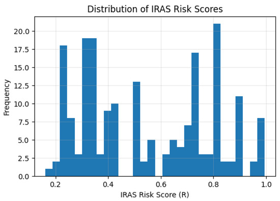  Figure 6. Distribution of IRAS risk scores based on calibrated vulnerability probabilities and normalized severity metrics.
  The contribution of each component is further illustrated in Figure 7. Exploitability and impact provide stable baseline contributions, while the calibrated vulnerability likelihood introduces dynamic variability that refines prioritization across instances. This demonstrates that IRAS integrates both learned probabilistic signals and standardized security metrics into a unified decision framework.
  

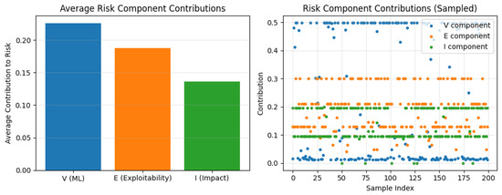  Figure 7. Decomposition of IRAS risk into vulnerability likelihood (V), exploitability (E), and impact (I). The left plot shows average contributions of each component, while the right plot illustrates sample-level variability. Exploitability and impact provide stable baseline risk, whereas the calibrated vulnerability likelihood introduces dynamic variability that refines prioritization across instances.
  Finally, the lifecycle effect of IRAS is shown in Figure 8. Unlike static and ML-only approaches, IRAS exhibits a consistent and earlier reduction in risk across SDLC phases. This behavior results from the integration of probabilistic predictions with structured risk factors, enabling continuous refinement of risk estimates and supporting proactive vulnerability mitigation throughout the lifecycle.
  

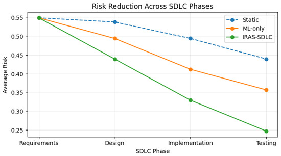  Figure 8. Average risk reduction across SDLC phases for static, ML-only, and IRAS-SDLC approaches. IRAS-SDLC achieves the steepest and earliest risk reduction, demonstrating the benefit of lifecycle-wide predictive risk estimation over implementation-only and static detection methods.

Nonlinear Risk Behavior

To capture interaction effects, the nonlinear IRAS formulation extends the linear model using coefficients $\delta =0.2$ and $\eta =0.2$, introducing interaction terms $(V·E)$ and $(V·I)$. Table 16 compares the range of linear and nonlinear risk scores based on the updated calibrated framework. While the minimum values remain close (0.16187 for the linear model and 0.16637 for the nonlinear model), the nonlinear formulation produces a significantly higher maximum risk value of 1.38818, reflecting the contribution of interaction effects between vulnerability likelihood and severity factors.

Table 16. Comparison of linear and nonlinear IRAS risk scores.

Metric	Linear (R)	Nonlinear (${\mathit{R}}_{\mathit{nl}}$)
Minimum	0.16187	0.16637
Maximum	0.99391	1.38818

Table 17 further illustrates representative high-risk cases, demonstrating that vulnerabilities with high vulnerability likelihood, exploitability, and impact experience noticeable amplification under the nonlinear model. In particular, instances where $V\approx 1$ and both E and I are high result in substantially increased $R_{nl}$ values compared to the linear score. This confirms that the nonlinear formulation effectively captures compound risk behavior while remaining grounded in the original probabilistic structure.

Table 17. Sample outputs of nonlinear risk amplification for high-risk vulnerabilities.

Sample	V	E	I	R	${\mathit{R}}_{\mathit{nl}}$
1	0.99651	1.00000	0.97826	0.99391	1.38818
2	0.99650	1.00000	0.97826	0.99390	1.38817
3	0.99650	1.00000	0.97826	0.99390	1.38817
4	0.99650	1.00000	0.97826	0.99390	1.38817
5	0.99648	1.00000	0.97826	0.99389	1.38815
6	0.99617	1.00000	0.97826	0.99374	1.38787
7	0.99542	1.00000	0.97826	0.99336	1.38721
8	0.99465	1.00000	0.97826	0.99298	1.38651
9	0.99651	1.00000	0.82609	0.96347	1.32742
10	0.99632	1.00000	0.82609	0.96338	1.32725

Figure 9 illustrates the relationship between linear and nonlinear risk scores. Most samples follow a near-linear trend along the diagonal, indicating that the overall structure of the risk distribution is preserved. However, clear deviations emerge for high-risk instances, where interaction terms introduce additional amplification. This demonstrates that the nonlinear model selectively emphasizes critical vulnerabilities without distorting lower-risk regions, thereby enhancing prioritization while maintaining interpretability.

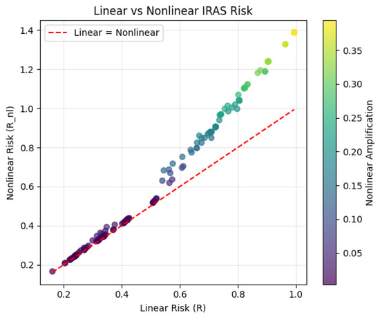
Figure 9. Comparison of linear and nonlinear IRAS risk scores. Points above the diagonal indicate nonlinear amplification, where interaction terms increase risk for high-severity vulnerabilities. Color intensity represents the magnitude of amplification while preserving the overall linear structure.

5.4. Lifecycle-Based Detection Latency and Remediation Cost Analysis

This section evaluates the lifecycle implications of IRAS-SDLC by quantifying detection latency and remediation cost across different detection paradigms. The theoretical modeling underpinning these comparisons, including phase assignment, latency formulation, and cost escalation factors, is presented in Section 4.3. The results below report the empirically computed outcomes under that framework.

Empirical Results

Table 18 and Table 19 summarize the computed latency and remediation cost across methods.

Table 18. Detection latency across methods.

Method	Latency (L)
Static	1
ML-based	0
IRAS-SDLC	−2

Table 19. Simulated remediation cost across methods.

Method	Cost (${\mathit{C}}_{\mathit{p}}$)
Static	10
ML-based	5
IRAS-SDLC	1

Figure 10 compares detection latency across methods, while Figure 11 illustrates the corresponding remediation cost.

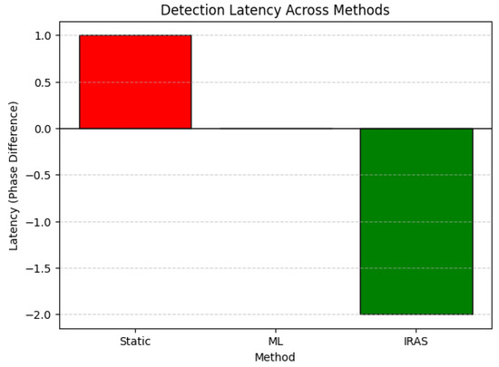
Figure 10. Detection latency across methods, showing earlier detection for IRAS-SDLC compared to ML-based and static approaches.

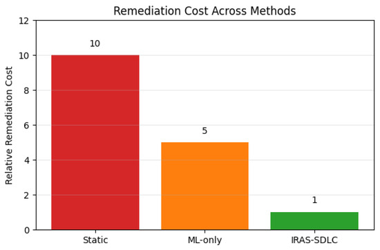
Figure 11. Simulated remediation cost across methods, illustrating the reduction in cost achieved through earlier detection in IRAS-SDLC.

The results show that IRAS-SDLC achieves the lowest latency and cost by enabling earlier detection. Static approaches incur the highest cost due to late-stage detection, while ML-based methods provide moderate improvement. These findings quantitatively validate that integrating risk assessment earlier in the SDLC leads to significant reductions in remediation effort.

5.5. Explainability Analysis

This section investigates the interpretability of the IRAS-SDLC framework by analyzing the contribution of code tokens to vulnerability predictions. The objective is to ensure that model decisions are transparent, auditable, and aligned with security-relevant programming patterns.

5.5.1. SHAP-Based Interpretation

To explain model predictions, SHAP (SHapley Additive exPlanations) is applied to the fine-tuned CodeBERT-based vulnerability classifier. SHAP estimates the contribution of each input token to the predicted vulnerability likelihood score V, enabling a fine-grained understanding of how different parts of the code influence model decisions.

Given the complexity of transformer-based architectures, a model-agnostic SHAP explainer is employed over raw code inputs. Due to the subword tokenization and masking mechanisms used in SHAP, token attributions may appear as fragmented or syntactic code elements rather than complete semantic units. To address this, token contributions are aggregated across a representative subset of samples and subsequently mapped to semantically meaningful programming constructs.

5.5.2. Feature Influence Analysis

Table 20 presents the most influential tokens identified through SHAP analysis. In contrast to earlier function-level interpretations, the updated results reveal that the model primarily relies on structural and memory-related programming constructs. The table includes both semantic interpretations and their associated security relevance, with importance values corresponding to normalized mean absolute SHAP contributions.

Table 20. SHAP-based feature importance with semantic and security-oriented interpretations.

Raw Token	Interpreted Token	Security Relevance	Importance
int	Integer declaration	Data type handling	1.00000
if (	Conditional control flow	Input validation logic	0.59396
static	Static storage	Memory persistence	0.59072
char *	Pointer manipulation	Memory access/buffer risk	0.59022
s−>	Structure field access	Pointer dereferencing	0.49801
long	Extended integer type	Numeric boundary handling	0.43910
struct	Structured memory layout	Memory organization	0.40350
return	Function control transfer	Execution flow correctness	0.39360
char *	Pointer usage	Memory safety	0.38876
s,	Parameter passing	Argument handling	0.37615
SSL *	Security API pointer	Cryptographic handling	0.26761
PHP_FUNCTION (	Framework interface	Input handling surface	0.26140
char **	Double pointer	Complex memory handling	0.25610
const	Immutable qualifier	Data integrity enforcement	0.24518
1;	Constant usage	Control termination	0.24278

Note: * denotes a pointer (variable storing a memory address), ** denotes a double pointer (pointer to a pointer), commonly used in C/C++ for dynamic memory management and buffer operations.

The identified tokens indicate that the model places significant emphasis on structural and memory-related programming patterns rather than relying solely on specific API calls. Tokens such as char *, struct, and pointer access patterns (e.g., s−>) highlight the importance of memory manipulation and data structure interactions, which are commonly associated with vulnerabilities such as memory corruption and improper access. Additionally, control flow constructs such as if ( and function-level elements like return suggest that the model captures logical validation and execution flow patterns.

This shift from function-specific tokens to structural representations indicates that the model learns generalized vulnerability patterns, improving its ability to detect previously unseen or obfuscated vulnerabilities.

Figure 12 provides a global visualization of token importance derived from SHAP values. The visualization highlights the relative contribution of top tokens, confirming that structural, control flow, and memory-related features dominate the model’s decision process.

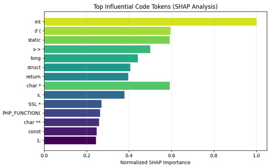
Figure 12. Top influential code tokens identified using SHAP. The model emphasizes structural and memory-related constructs (* denotes a pointer, ** denotes a double pointer), control flow statements, and data structure access, which are commonly associated with vulnerability-prone code regions.

5.5.3. Governance Implications

The explainability results support key security and governance objectives, as summarized in Table 21.

Table 21. Governance implications of SHAP-based explainability in IRAS-SDLC.

Aspect	Implication
Interpretability	The model provides human-understandable explanations by linking predictions to structural code patterns such as memory access, pointer usage, and control flow constructs.
Auditability	Token-level attribution enables verification of model decisions, allowing analysts to trace predictions back to specific code patterns and supporting compliance with security auditing requirements.
RMF Alignment	The ability to trace risk predictions to interpretable code-level features supports RMF principles, enabling transparent risk justification, prioritization, and informed decision-making.

The SHAP-based analysis demonstrates that IRAS-SDLC not only produces accurate risk estimates but also provides interpretable insights grounded in structural vulnerability patterns. This enhances trust, supports governance requirements, and enables the framework to generalize beyond specific known vulnerability signatures, making it suitable for security-critical and compliance-driven environments.

5.5.4. Runtime Risk Adaptation Under Zero Trust

To extend IRAS-SDLC beyond development phases, runtime risk adaptation is incorporated using anomaly-driven feedback. In this setting, vulnerability risk is continuously updated based on observed system behavior, aligning with Zero Trust principles where trust is not static but dynamically evaluated.

Let $A\in [0,1]$ denote a normalized anomaly score derived from runtime telemetry. The adjusted risk is defined as

$$R_{\mathrm{runtime}}=(1-\theta )R+\theta A$$

where $\theta \in [0,1]$ controls the influence of runtime observations. This formulation preserves boundedness while enabling dynamic adjustment of risk based on real- time evidence.

Figure 13 illustrates the relationship between baseline IRAS risk and runtime-adjusted risk. The diagonal reference line represents the case where no runtime adaptation occurs. Points above the line indicate increased risk due to anomalous system behavior, while points below indicate reduced risk under normal operational conditions.

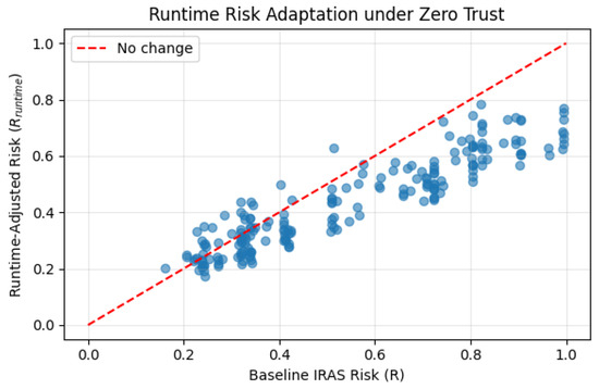
Figure 13. Runtime risk adaptation under Zero Trust, showing how anomaly signals dynamically adjust IRAS risk scores during system operation. Blue points represent runtime-adjusted risk; the red dashed diagonal indicates no runtime adjustment ($R_{\mathrm{runtime}}=R$).

The results show that risk estimates are not fixed after deployment but are continuously refined based on runtime observations. In particular, anomaly signals can elevate risk for potentially exploited vulnerabilities or reduce risk when system behavior remains stable. This demonstrates that IRAS-SDLC supports continuous, evidence-driven risk assessment throughout the operational lifecycle.

By integrating runtime feedback with development-phase risk modeling, IRAS-SDLC closes the loop between prediction and observation, providing a unified framework that aligns with Zero Trust security principles.

5.6. Statistical Validation

This section presents the statistical validation of the IRAS-SDLC framework, focusing on the robustness of the learned vulnerability likelihood component (V) under dataset shift. Cross-domain generalization is evaluated using the Juliet Test Suite [35], containing synthetic C/C++ and Java programs with documented CWE classifications, enabling controlled validation across programming languages and code structures. The objective is not to benchmark CodeBERT in isolation, but to assess the stability of V within the IRAS risk aggregation framework, following the methodology outlined in Section 4 and Section 4.9.

5.6.1. Confidence Intervals and Cross-Domain Generalization Analysis

Since IRAS-SDLC is intended for deployment across heterogeneous codebases and development contexts, assessing the robustness of the learned vulnerability likelihood (V) under dataset shift is essential for validating the overall framework. The pretrained CodeBERT model is therefore evaluated on two Juliet subsets: Juliet-C (function-level, structurally aligned with training data) and Juliet-Java (file-level, cross-language and cross-granularity). Performance is measured using F1 and ROC-AUC with 95% confidence intervals via bootstrap resampling, summarized in Table 22.

Table 22. Performance and 95% confidence intervals across datasets under domain shift.

Dataset	F1	F1 CI	ROC-AUC	ROC CI
Juliet-C	0.1951	[0.1750, 0.2128]	0.6143	[0.5975, 0.6300]
Juliet-Java	0.7477	[0.7368, 0.7581]	0.4732	[0.4575, 0.4883]

For Juliet-C, the model retains moderate ranking capability (ROC-AUC ≈ 0.61) but exhibits low F1 (≈0.20), reflecting limited discriminative power under domain shift. For Juliet-Java, the high F1 (≈0.75) is driven by class imbalance rather than genuine discrimination, confirmed by the near-random ROC-AUC (≈0.47). Evaluation on balanced subsets confirms this degradation persists, indicating a systematic consequence of cross-language and cross-representation shift.

These findings confirm that V alone does not generalize reliably across substantial distribution shifts, directly motivating the IRAS-SDLC aggregation approach. By combining V with exploitability (E) and impact (I), IRAS mitigates this instability and provides a more robust basis for cross-domain risk assessment.

5.6.2. ANOVA Analysis of Detection Latency and Remediation Cost

To evaluate whether differences across methods are statistically significant, a one-way ANOVA is conducted on detection latency and remediation cost for Static, ML-only, and IRAS approaches. Since values are defined at the method level, empirical distributions are generated by introducing small stochastic variations to reflect realistic variability across instances. The ANOVA results are presented in Table 23.

Table 23. ANOVA results for detection latency and remediation cost across methods.

Metric	F-Statistic	p-Value
Latency	47,937.996	<0.001
Cost	16,271.954	<0.001

The large F-statistics and p-values below 0.001 confirm statistically significant differences across all methods. IRAS achieves the lowest latency and cost through early-phase detection, while static analysis incurs the highest values due to late-stage identification, and ML-based detection provides moderate improvement at implementation time.

5.6.3. Effect Size Results

While ANOVA establishes statistical significance, it does not quantify the magnitude of differences. Cohen’s d is therefore computed for pairwise comparisons between Static, ML-only, and IRAS approaches, where values of $d=0.2$, $0.5$, and $0.8$ correspond to small, medium, and large effects respectively. The effect size results are shown in Table 24.

Table 24. Effect size (Cohen’s d) for latency and cost across methods.

Metric	Static vs. ML	Static vs. IRAS	ML vs. IRAS
Latency	10.0670	29.3248	21.3393
Cost	9.8392	18.2808	8.0197

All comparisons yield consistently large effect sizes, with IRAS producing the largest values in both metrics. While the magnitude is partly influenced by the structured nature of phase-based modeling, the results confirm that IRAS-SDLC improvements are not only statistically significant but practically meaningful in terms of detection latency and remediation cost reduction.

5.6.4. Survival Analysis of Detection Timing

To further analyze detection behavior across the software development lifecycle, survival analysis is employed by modeling vulnerability detection as a time-to-event process. In this context, the event corresponds to the detection of a vulnerability, and time is represented by the SDLC phase in which detection occurs.

Detection times are derived from the phase-based modeling defined in Section 4, where earlier lifecycle stages correspond to lower time values. Kaplan–Meier estimators are used to compare detection curves across static, ML-only, and IRAS methods.

The resulting detection curves are illustrated in Figure 14. The curves represent the probability that a vulnerability remains undetected as a function of detection time.

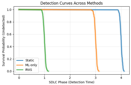
Figure 14. Kaplan–Meier detection curves showing the probability of vulnerabilities remaining undetected over SDLC phases. Earlier declines indicate faster detection. IRAS demonstrates the earliest detection behavior, followed by ML-only and static approaches.

As shown in Figure 14, the IRAS curve exhibits the earliest and most rapid decline, indicating that vulnerabilities are detected at earlier stages of the lifecycle. The ML-only approach shows a moderate decline, while static methods exhibit the slowest decrease, reflecting delayed detection. The horizontal separation between the curves highlights the shift in detection timing across methods. In particular, the leftward position of the IRAS curve indicates earlier detection, while the rightward shift of the static curve reflects later identification during testing phases.

A log-rank test further confirms that the differences between detection curves are statistically significant ($p<0.005$), supporting the observed separation across methods. The survival analysis provides a temporal perspective that complements the statistical results presented earlier. It shows that IRAS-SDLC not only reduces average detection latency but also consistently enables earlier detection across the lifecycle.

6. Discussion

This section interprets the experimental findings across three dimensions: the limitations of implementation-only detection, the advantages of lifecycle risk aggregation, and the practical applicability of IRAS-SDLC. The connection between empirical results and the theoretical framework is also examined.

6.1. Limits of Implementation-Only Detection

Transformer-based models such as CodeBERT achieve strong vulnerability classification performance, yet operate strictly at the implementation phase without awareness of the broader lifecycle. Implementation-only detection does not account for lifecycle-dependent cost escalation or detection latency, meaning vulnerabilities identified during coding or testing may have already propagated through system design, increasing remediation complexity. While accurate, these models remain reactive and do not support proactive lifecycle decision-making.

6.2. Advantage of Lifecycle Risk Aggregation

IRAS-SDLC extends vulnerability detection by integrating predictive outputs with exploitability and impact into a unified risk representation. The aggregation of V, E, and I improves decision quality in two ways: it reduces false urgency by preventing low-impact, high-confidence vulnerabilities from being over-prioritized, and it mitigates missed threats by elevating vulnerabilities with high exploitability or impact even when model confidence is low. The lifecycle-integrated formulation further enables proactive mitigation before vulnerabilities propagate into later phases.

6.3. Practical Applicability

IRAS-SDLC is designed for direct integration into real-world secure development environments. In a DevSecOps pipeline, the framework operates as a risk scoring layer embedded within CI/CD workflows, consuming commit-time vulnerability predictions and CVSS-derived metrics to produce phase-indexed risk scores that trigger prioritized remediation actions. Security engineers can use the risk-to-decision mapping defined in Table 13 to route flagged components to appropriate response workflows without manual triage. In RMF-governed environments such as federal agencies or defense contractors, the framework generates machine-verifiable compliance artifacts at each SDLC phase, supporting Continuous Authorization to Operate requirements. The SHAP-based explainability layer ensures that risk decisions are traceable to specific code-level features, satisfying audit and regulatory transparency requirements.

Under Zero Trust architectures, the runtime risk adaptation mechanism allows security posture to be dynamically adjusted based on operational telemetry, bridging development-time assurance with operational security monitoring. These properties make IRAS-SDLC applicable across enterprise software development, critical infrastructure systems, and cloud-native environments where continuous, governance-aligned risk assessment is required.

6.4. Interpretation of Results

IRAS-SDLC achieves earlier detection, reduced latency, and lower remediation cost compared to static and implementation-only approaches by shifting detection to earlier SDLC phases. Negative detection latency reflects the ability to identify risk prior to the point of vulnerability introduction, directly reducing remediation cost through the phase-dependent escalation model. Risk stabilization is achieved through the bounded and convex aggregation of V, E, and I, reducing variance and avoiding over-reliance on any single signal. These results confirm that machine learning alone is insufficient for lifecycle-aware security without incorporating exploitability, impact, and lifecycle timing.

6.5. Connection to Theoretical Framework

The empirical findings are consistent with the theoretical models introduced earlier. Latency reduction aligns with the phase-indexed formulation $L=t_d-t_i$, and cost reduction reflects the escalation model $C_p={\lambda }_p{C}_b$, where earlier phases incur lower overhead. The stability and interpretability of risk scores are supported by the monotonicity, convexity, and boundedness properties of $R=\alpha V+\beta E+\gamma I$, ensuring consistent prioritization across vulnerabilities and SDLC phases.

7. Limitations

Several limitations should be acknowledged. First, parts of the evaluation rely on theoretical modeling and simulation of lifecycle behavior, particularly for detection latency and remediation cost. While grounded in established software engineering principles, these results do not fully capture real-world pipeline variability.

Second, dataset alignment between Big-Vul and NVD introduces potential inconsistencies, as not all predicted vulnerabilities can be directly mapped to CVE records. This may affect the precision of integrated risk variables.

Third, the generalization analysis reveals performance degradation under cross-language and cross-granularity conditions, as observed in the Juliet-Java dataset. This highlights limitations in the transferability of learned vulnerability representations.

Finally, the framework is evaluated in a simulated DevSecOps setting without deployment in a real CI/CD pipeline. As a result, operational overhead, integration complexity, and real-time performance considerations are not fully assessed.

8. Threats to Validity

Several threats to validity should be considered when interpreting the results. Internal validity may be affected by assumptions in the experimental setup, particularly in the modeling of detection latency and remediation cost. Although these formulations are grounded in established software engineering principles, they rely on simulated phase assignments rather than direct observation in real-world development environments.

External validity is influenced by the choice of datasets. While multiple datasets, including Big-Vul, Devign, NVD, and Juliet, are used to improve coverage, they may not fully represent all programming languages, system architectures, or industrial practices. The observed degradation in cross-language scenarios further highlights limitations in generalization.

Construct validity is associated with how vulnerability risk is defined and measured. The IRAS formulation combines predicted vulnerability likelihood with CVSS-based exploitability and impact metrics, which are widely accepted but may not capture all contextual or environment-specific risk factors.

Conclusion validity is supported through statistical testing, including ANOVA, effect size analysis, and survival modeling. However, the strong statistical significance observed may be influenced by controlled experimental conditions and large sample sizes, which may differ from real-world variability.

9. Conclusions and Future Work

This work demonstrates that integrating predictive intelligence across the SDLC fundamentally shifts vulnerability detection from reactive to proactive.

The results establish a clear progression across detection paradigms. Static analysis provides limited effectiveness due to its reliance on predefined rules. Machine learning-based detection achieves strong predictive performance but remains confined to the implementation phase and lacks lifecycle awareness. In contrast, the proposed IRAS-SDLC framework extends detection into a lifecycle-aware, decision-driven process by integrating predictive modeling with quantitative risk aggregation and governance alignment. By combining vulnerability likelihood, exploitability, and impact into a unified formulation, IRAS-SDLC enables earlier detection, reduced latency, and significantly lower remediation cost. These improvements are statistically significant and consistent across classification, timing, and cost-based evaluation metrics. Overall, the findings demonstrate that effective software assurance requires not only accurate detection, but also lifecycle integration and structured risk reasoning to support prioritization and decision-making.

Future work will extend the IRAS-SDLC framework along three key directions. From a modeling perspective, future research will explore nonlinear risk learning and adaptive estimation of weighting parameters $(\alpha ,\beta ,\gamma )$ to better capture interactions between vulnerability likelihood, exploitability, and impact. From a system integration perspective, the framework will be deployed within real-world DevSecOps environments, including CI/CD pipelines and real-time security monitoring systems, to evaluate operational performance and integration overhead. From an intelligence perspective, further enhancements will incorporate reinforcement learning for adaptive decision policies and improved explainability techniques to strengthen interpretability and support automated remediation strategies.

References

- National Institute of Standards and Technology. National Vulnerability Database Data Feeds. In NVD Data Repository; National Institute of Standards and Technology: Gaithersburg, MD, USA, 2023. [Google Scholar]
- OWASP Foundation. OWASP Top 10: The Ten Most Critical Web Application Security Risks. In OWASP Foundation Report; OWASP Foundation: Wilmington, DE, USA, 2021. [Google Scholar]
- Boehm, B.W. Software Engineering Economics; Prentice Hall: Englewood Cliffs, NJ, USA, 1981. [Google Scholar]
- Rahim, E.; Burrell, D.N. Integrating Software Assurance into the Software Development Life Cycle (SDLC). J. Inf. Syst. Technol. Plan. 2010, 3, 49–53. [Google Scholar]
- Kindervag, J.; Balaouras, S.; Mak, K.; Blackborow, J. No More Chewy Centers: Introducing the Zero Trust Model of Information Security; Forrester Research: Cambridge, MA, USA, 2010. [Google Scholar]
- Rose, S.; Borchert, O.; Mitchell, S.; Connelly, S. Zero Trust Architecture; NIST Special Publication 800-207; National Institute of Standards and Technology: Gaithersburg, MD, USA, 2020.
- National Security Agency. Embracing a Zero Trust Security Model. In NSA Cybersecurity Information Sheet; National Security Agency: Ft. Meade, MD, USA, 2021. Available online: https://media.defense.gov/2021/Feb/25/2002588479/-1/-1/0/CSI_EMBRACING_ZT_SECURITY_MODEL_UOO115131-21.PDF (accessed on 6 March 2026).
- Cybersecurity and Infrastructure Security Agency. Zero Trust Maturity Model Version 2.0. In CISA Report; Cybersecurity and Infrastructure Security Agency: Washington, DC, USA, 2023. Available online: https://www.cisa.gov/zero-trust-maturity-model (accessed on 6 March 2026).
- Rajapakse, R.N.; Zahedi, M.; Babar, M.A.; Shen, H. Challenges and solutions when adopting DevSecOps: A systematic review. Inf. Softw. Technol. 2022, 141, 106700. [Google Scholar] [CrossRef]
- Rafi, S.; Yu, W.; Akbar, M.A.; Alsanad, A.; Gumaei, A. Prioritization Based Taxonomy of DevOps Security Challenges Using PROMETHEE. IEEE Access 2020, 8, 105426–105446. [Google Scholar] [CrossRef]
- Mahmood, S.; Niazi, M.; Alshayeb, M. Security in DevOps: A Systematic Mapping Study. In Proceedings of the ENASE, Prague, Czech Republic, 5–6 May 2020. [Google Scholar]
- Li, Z.; Zou, D.; Xu, S.; Ou, X.; Jin, H.; Wang, S.; Deng, Z. VulDeePecker: A Deep Learning-Based System for Vulnerability Detection. In Proceedings of the Network and Distributed System Security Symposium, San Diego, CA, USA, 18–21 February 2018. [Google Scholar]
- Zhou, Y.; Liu, S.; Siow, J.; Du, X.; Liu, Y. Devign: Effective Vulnerability Identification by Learning Comprehensive Program Semantics via Graph Neural Networks. In Proceedings of the Advances in Neural Information Processing Systems, Vancouver, BC, Canada, 8–14 December 2019. [Google Scholar]
- Feng, Z.; Guo, D.; Tang, D.; Duan, N.; Feng, X.; Gong, M.; Shou, L.; Qin, B.; Liu, T.; Jiang, D.; et al. CodeBERT: A Pre-Trained Model for Programming and Natural Languages. In Proceedings of the Findings of the Association for Computational Linguistics, Online, 16–20 November 2020. [Google Scholar]
- Shin, Y.; Meneely, A.; Williams, L.; Osborne, J.A. Evaluating Complexity, Code Churn, and Developer Activity Metrics as Indicators of Software Vulnerabilities. IEEE Trans. Softw. Eng. 2011, 37, 772–787. [Google Scholar] [CrossRef]
- Dempsey, K.L.; Johnson, L.A.; Scholl, M.A.; Stine, K.M.; Jones, A.C.; Orebaugh, A.; Chawla, N.S.; Johnston, R. Information Security Continuous Monitoring for Federal Information Systems and Organizations; NIST Special 1166 Publication 800-137; National Institute of Standards and Technology: Gaithersburg, MD, USA, 2011.
- Force, J.T. Risk Management Framework for Information Systems and Organizations; NIST Special Publication 800-37 Revision 2; National Institute of Standards and Technology: Gaithersburg, MD, USA, 2018.
- Department of Defense CIO. Memorandum: Continuous Authorization to Operate (cATO); U.S. Department of Defense: Washington, DC, USA, 2022. Available online: https://media.defense.gov/2022/Feb/03/2002932852/-1/-1/0/CONTINUOUS-AUTHORIZATION-TO-OPERATE.PDF (accessed on 6 March 2026).
- Humble, J.; Farley, D. Continuous Delivery: Reliable Software Releases Through Build, Test, and Deployment Automation; Addison-Wesley: Boston, MA, USA, 2010. [Google Scholar]
- Myrbakken, H.; Colomo-Palacios, R. DevSecOps: A Multivocal Literature Review. In Proceedings of the International Conference on Software Process Improvement and Capability Determination (SPICE), Palma de Mallorca, Spain, 4–5 October 2017. [Google Scholar]
- Ur Rahman, A.A.; Williams, L. Software Security in DevOps: Synthesizing Practitioners’ Perceptions and Practices. In Proceedings of the IEEE Secure Development Conference, Virtual, 28–30 September 2020. [Google Scholar]
- Fu, M.; Lyu, M.R.; Lou, J.G. AI for DevSecOps: A Landscape and Future Opportunities. arXiv 2024, arXiv:2404.10173. [Google Scholar] [CrossRef]
- Pandey, P.; Katsikas, S. The Future of Cyber Risk Management: AI and DLT for Automated Cyber Risk Modelling. In Handbook of Research on Artificial Intelligence, Innovation and Entrepreneurship; Edward Elgar Publishing: Cheltenham, UK, 2023. [Google Scholar]
- Cox, J.; Bird, C.; Rahman, F. Measuring Dependency Freshness in Software Systems. In Proceedings of the International Conference on Software Engineering, Montreal, QC, Canada, 25–26 May 2019. [Google Scholar]
- Zhang, Q.; Chen, M.; Li, L. Security and Privacy in Cloud Microservices. In Proceedings of the IEEE Cloud Computing, San Francisco, CA, USA, 2–7 July 2018. [Google Scholar]
- Fu, M.; Tantithamthavorn, C. LineVul: A Transformer-Based Line-Level Vulnerability Prediction System. In Proceedings of the IEEE Transactions on Software Engineering; Association for Computing Machinery: New York, NY, USA, 2022. [Google Scholar]
- Kanade, A.; Maniatis, P.; Balakrishnan, G.; Shi, K. Learning and Evaluating Contextual Embedding of Source Code. In International Conference on Machine Learning; PMLR: New York, NY, USA, 2020. [Google Scholar]
- Omar, M.; Shiaeles, S. VulDetect: A novel technique for detecting software vulnerabilities using language models. In Proceedings of the 2023 IEEE International Conference on Cyber Security and Resilience (CSR), Venice, Italy, 31 July–2 August 2023. [Google Scholar]
- Allamanis, M.; Barr, E.T.; Devanbu, P.; Sutton, C. A Survey of Machine Learning for Big Code and Naturalness. ACM Comput. Surv. 2018, 51, 1–37. [Google Scholar] [CrossRef]
- Pearce, H.; Ahmad, B.; Tan, B.; Dolan-Gavitt, B.; Karri, R. Asleep at the Keyboard: Assessing the Security of GitHub Copilot’s Code Contributions. In Proceedings of the IEEE Symposium on Security and Privacy Workshops, San Francisco, CA, USA, 22–26 May 2022. [Google Scholar]
- Chen, M.; Tworek, J.; Jun, H.; Yuan, Q.; Pinto, H.P.D.O.; Kaplan, J.; Edwards, H.; Burda, Y.; Joseph, N.; Brockman, G.; et al. Evaluating Large Language Models Trained on Code. arXiv 2021, arXiv:2107.03374. [Google Scholar] [CrossRef]
- Althar, R.R.; Samanta, D.; Kaur, M.; Singh, D.; Lee, H.N. Automated Risk Management Based Software Security Vulnerabilities Management. IEEE Access 2022, 10, 90597–90608. [Google Scholar] [CrossRef]
- Bottou, L.; Curtis, F.E.; Nocedal, J. Optimization Methods for Large-Scale Machine Learning. SIAM Rev. 2018, 60, 223–311. [Google Scholar] [CrossRef]
- Fan, X.; Li, Y.; Wang, Y.; Jin, Z. A Large-Scale Dataset for Vulnerability Detection in Open-Source Code. In Proceedings of the IEEE International Conference on Software Maintenance and Evolution, Adelaide, Australia, 27 September–3 October 2020. [Google Scholar]
- National Security Agency (NSA); NIST. Juliet Test Suite for C/C++ and Java. In NIST Software Assurance Reference Dataset; National Security Agency (NSA): Fort Meade, MD, USA; NIST: Gaithersburg, MD, USA, 2017. [Google Scholar]
- Johnson, B.; Song, Y.; Murphy-Hill, E.; Bowdidge, R. Why Don’t Software Developers Use Static Analysis Tools to Find Bugs? In Proceedings of the International Conference on Software Engineering, San Francisco, CA, USA, 18–26 May 2013. [Google Scholar]
- Ayewah, N.; Pugh, W.; Hovemeyer, D.; Morgenthaler, J.D.; Penix, J. Using Static Analysis to Find Bugs. IEEE Softw. 2008, 25, 22–29. [Google Scholar] [CrossRef]
- Fawcett, T. An Introduction to ROC Analysis. Pattern Recognit. Lett. 2006, 27, 861–874. [Google Scholar] [CrossRef]
- Powers, D.M. Evaluation: From Precision, Recall and F-Measure to ROC, Informedness, Markedness & Correlation. J. Mach. Learn. Technol. 2011, 2, 37–63. [Google Scholar]
Disclaimer/Publisher’s Note: The statements, opinions and data contained in all publications are solely those of the individual author(s) and contributor(s) and not of MDPI and/or the editor(s). MDPI and/or the editor(s) disclaim responsibility for any injury to people or property resulting from any ideas, methods, instructions or products referred to in the content. |
© 2026 by the authors. Licensee MDPI, Basel, Switzerland. This article is an open access article distributed under the terms and conditions of the Creative Commons Attribution (CC BY) license.