A Multi-Step Interval-Valued Carbon Price Forecasting System Based on Multi-Source Mixed-Frequency Information Modeling

Abstract

Accurate carbon price forecasting is essential for market stability, regulatory assessment, and risk management in emission trading systems. However, existing approaches find it challenging to extract informative signals from high-dimensional multi-source data, integrate mixed-frequency influencing factors, and maintain robustness in multistep forecasting. This study proposes a unified multi-step interval-valued carbon price forecasting system that integrates a multi-objective reinforcement learning (MORL)-based mechanism for feature selection, a multi-source mixed-frequency data sampling (M-MIDAS) module, and a leading-expert dynamic residual correction network (LE-DRCN). MORL performs adaptive feature selection by jointly considering multiscale temporal characteristics and feature redundancy. M-MIDAS aligns multi-source heterogeneous factors into a unified representation, whereas LE-DRCN captures structured residual patterns and dynamically adjusts expert contributions through attention-based integration, thereby improving forecasting accuracy and stability across horizons. The proposed system consistently outperforms benchmark models in multistep forecasting on China Emission Allowance market data. Ablation analysis confirmed the importance of mixed-frequency representation and dynamic residual correction, and statistical tests further verified the robustness of the performance gains. Interpretability analysis revealed horizon-dependent expert contributions, reflecting adaptive model behavior under varying market conditions. Overall, the proposed system provides a robust and interpretable solution for multi-step interval-valued carbon price forecasting under complex multi-source and mixed-frequency environments.

1. Introduction

1.1. Background

Carbon markets have gradually evolved into complex adaptive systems characterized by pronounced uncertainty, multisource interactions, and nonlinear dynamics. Within the framework of the Emissions Trading System (ETS), which has been widely recognized as a cost-effective policy instrument for mitigating climate change and has been adopted in many countries and regions [1], such complexity creates significant challenges for market management and decision-making. In this context, accurate carbon price forecasting is highly important for maintaining the stability and efficiency of the ETS, because it supports compliance planning, investment decisions, regulatory assessment, allowance allocation, and financial risk pricing [2]. This importance has further increased because of ongoing institutional changes, including market expansion and the gradual transition from intensity-based targets to absolute emission caps. As a result, carbon price dynamics are increasingly shaped by the joint effects of macroeconomic conditions, policy interventions, market fundamentals, and investor sentiment [3].

Carbon prices exhibit strong temporal variability, making multi-step forecasting essential for capturing evolving market dynamics under changing regulatory and macroeconomic environments. In forecasting literature, point-based approaches typically focus on estimating a single representative price value at each horizon, which may be insufficient to characterize the full distributional behavior of carbon price movements [4]. To address this limitation, this study formulates the problem as a multi-step interval-valued carbon price forecasting task. Unlike point forecasting, which provides a scalar prediction for each future time step, interval-valued forecasting directly models the lower and upper price components at each forecasting horizon, thereby representing each future observation as a structured pair rather than a single value [5]. This formulation is particularly relevant in carbon markets, where policy interventions, energy price shocks, and macroeconomic fluctuations often asymmetrically affect downside and upside price dynamics, leading to heterogeneous responses at different horizons. These characteristics pose substantial challenges for developing accurate multi-step forecasting systems. Therefore, this study focuses on multi-step interval-valued carbon price forecasting based on data from the CEA market, aiming to improve predictive accuracy and provide a more comprehensive characterization of complex market dynamics under multi-source heterogeneous influencing factors in a unified system.

1.2. Literature Review

Previous studies have extensively employed traditional econometric models for carbon price analysis and forecasting. For example, the generalized autoregressive conditional heteroskedasticity (GARCH) family of models has been widely used to characterize volatility dynamics in carbon markets, and Liu et al. [6] applied a GARCH-based framework to examine key features of carbon price returns. To jointly model the mean and variance processes, Huang et al. [7] developed an autoregressive integrated moving average (ARIMA)-GARCH model that incorporates the operational characteristics of carbon credit mechanisms and external influencing factors. In addition, Yang et al. [8] used a vector autoregression model to investigate the dynamic interactions between carbon price liquidity and stock market liquidity. Although these econometric models provide a solid theoretical basis for describing linear dependence and volatility clustering, their restrictive assumptions often limit their ability to capture the nonlinear and non-stationary features of carbon market data.

To overcome these limitations, recent studies have increasingly turned to artificial intelligence techniques. For instance, Luo et al. [9] proposed a text-driven forecasting framework based on weighted interval-joint quadratic support vector regression to incorporate investor sentiment into interval carbon price prediction. Zhu et al. [10] developed a robust prediction system combining a probability density recurrence network and an interval multi-layer perceptron to generate interval-valued forecasts. Mu et al. [11] further proposed a multi-source forecasting framework based on Long Short-Term Memory networks to improve carbon price prediction accuracy. Building on these advances, some studies have moved beyond single-model AI forecasting toward hybrid paradigms that integrate complementary modeling techniques. Li et al. [12] developed a dual decomposition and error-correction framework for carbon price forecasting, showing that combining decomposition, prediction, and residual correction can further improve predictive accuracy. These studies show that hybrid modeling can improve predictive performance by combining different techniques to capture distinct aspects of carbon price dynamics [13]. However, hybrid models are typically built around a limited number of pre-specified components, which may still constrain their ability to fully exploit the diversity of multiple candidate predictors.

Against this background, ensemble learning has emerged as a more general paradigm for integrating the strengths of multiple forecasting models [14]. For example, Sha et al. [15] employed the Grey Wolf Optimization algorithm to derive optimal weights for multiple forecasting models. However, most conventional ensemble methods combine model outputs only at the final prediction stage, treating the forecasts of different models as parallel inputs and paying limited attention to the systematic errors left unexplained by the primary predictor [16]. To address this limitation, some recent studies have moved from direct forecast combination to residual-driven learning schemes, in which a primary predictor first generates a primary forecast and auxiliary models are then used to model the remaining unexplained components [17]. This transition reflects a growing emphasis on structured ensemble design, where the interaction among sub-models is explicitly organized rather than simply aggregated at the output level.

Beyond improvements in model architecture, recent studies have extended carbon price forecasting from single-step point prediction to multi-step point prediction and interval-valued prediction, enabling a richer characterization of temporal dynamics and market uncertainty [18]. For example, prior work has explored multi-step forecasting frameworks, while others have focused on interval-valued prediction to quantify uncertainty. However, multi-step interval-valued carbon price forecasting remains largely unexplored, despite its increasing practical relevance. As forecasting tasks shift toward multi-step and interval-valued settings, the difficulty of prediction increases due to error accumulation over time and the need to explicitly model uncertainty propagation [19]. These characteristics require models to learn more informative and comprehensive representations of underlying market dynamics.

Under such conditions, relying on a limited set of explanatory variables is often insufficient. This necessitates the incorporation of diverse and complementary information sources. Carbon price dynamics are jointly influenced by economic, financial, policy-related, and sentiment factors, making multi-source data integration essential for accurate prediction. However, the introduction of multi-source data fundamentally changes the structure of the modeling problem. On the one hand, it significantly expands the feature space, leading to redundancy and noise among variables. On the other hand, these heterogeneous data sources are often observed at different temporal frequencies, resulting in mixed-frequency heterogeneity. Feature selection methods such as the least absolute shrinkage and selection operator (LASSO) and importance-based screening are commonly adopted to address the high-dimensional nature of multi-source inputs [20]. However, these approaches typically rely on simple selection criteria and fail to capture nonlinear interactions among heterogeneous variables, limiting their effectiveness in complex multi-source environments [21]. The mixed-frequency data sampling (MIDAS) framework has been introduced to handle mixed-frequency data by incorporating high-frequency variables into low-frequency models without temporal aggregation, thereby preserving fine-grained temporal information [22]. For example, Liu et al. [23] employed a GARCH-MIDAS model incorporating economic policy uncertainty indices to forecast EU carbon futures volatility and reported improved predictive accuracy.

Despite these advances, existing approaches typically address high-dimensional feature selection and mixed-frequency modeling as separate components. In particular, most MIDAS-based methods are restricted to single high-frequency predictors or treat multiple variables independently, which prevents them from capturing cross-source interactions in multi-source mixed-frequency settings. This limitation becomes more critical in multi-step interval forecasting, where error accumulation and uncertainty propagation further increase the demand for coordinated modeling of heterogeneous information. To overcome these limitations, this study develops a unified multi-source frequency alignment and feature selection framework that enables joint modeling and coherent integration of heterogeneous high-frequency factors within a multi-step interval forecasting system.

1.3. Research Gaps

A systematic review of the existing literature revealed several persistent limitations from a systems science perspective. The current approaches remain fragmented and fail to capture the carbon market as a complex adaptive system. Specifically, this study identified the following research gaps:

(1) Lack of a dynamic feature selection paradigm capable of reconciling competing objectives in multi-source data-driven carbon price forecasting. Most existing methods adopt static selection strategies, making it difficult to jointly capture short-term fluctuations and long-term structural information, while also limiting their ability to distinguish informative signals from redundant features in high-dimensional inputs.

(2) Insufficient modeling capability for multi-step forecasting with multi-source mixed-frequency data. The effective utilization of heterogeneous mixed-frequency information across multiple horizons remains challenging, particularly for capturing the joint dynamics of price fluctuations.

(3) Structural limitations in conventional mixed-frequency models in multi-source contexts. Conventional mixed-frequency models are inherently limited in multisource settings because they are typically designed to accommodate only a single high-frequency explanatory variable. This prevents the joint integration of heterogeneous information such as market, macroeconomic, and sentiment data, limiting their ability to capture high-dimensional feature interactions.

(4) Limitations in existing residual correction and ensemble systems. Existing approaches rely on static combination schemes, overlooking the dynamic relationship between collective forecast distributions and baseline residuals, and constraining the effectiveness of error correction.

(5) Limited interpretability in multi-source mixed-frequency forecasting systems. There is still insufficient understanding of how different input factors and model components contribute to predictions across forecasting horizons, making it difficult to interpret the roles of multi-source drivers and the dynamics of model behavior.

1.4. Main Work and Contributions

To address the above research gaps, this study developed a multistep interval-valued carbon price forecasting system based on multisource mixed-frequency information modeling. The proposed system is designed to address three key challenges in carbon price forecasting: (1) the adaptive identification of informative and non-redundant drivers in high-dimensional multisource data, (2) the coherent fusion of multisource information observed at different temporal frequencies for unified forecasting, and (3) how to dynamically correct structured residual errors and enable adaptive interaction among expert models in multi-step interval-valued forecasting. Specifically, a multi-objective reinforcement learning (MORL) mechanism was developed to perform adaptive feature selection, thereby enabling the extraction of informative and non-redundant drivers from high-dimensional multi-source data. A multi-source MIDAS (M-MIDAS) module was then constructed to coherently integrate heterogeneous factors with different temporal frequencies, providing a unified representation for multistep forecasting. Finally, the leading-expert dynamic residual correction network (LE-DRCN) was introduced to capture structured residual patterns and dynamically adjust expert contributions, thereby improving prediction accuracy and robustness under changing market conditions. The empirical results demonstrate that the proposed system consistently outperforms benchmark models, indicating its effectiveness as a practical tool for multistep carbon price forecasting. The main contributions of this study are as follows:

(1) A novel multi-step interval-valued ensemble forecasting system was developed. The proposed system enables the joint forecasting of the highest and lowest carbon prices across multiple horizons and provides a unified architecture for integrating feature selection, mixed-frequency representation, and ensemble learning.

(2) A multidimensional feature optimization mechanism driven by MORL was constructed. Guided by a novel tripartite reward function that balances high-frequency dynamic values, low-frequency trend values, and negative maximum redundancy, this mechanism automatically extracts the core drivers while circumventing the curse of dimensionality.

(3) A mixed-frequency modeling mechanism was developed to enable multi-source heterogeneous information fusion, in which the proposed M-MIDAS aggregates multiple high-frequency information streams into a unified low-frequency representation. Unlike traditional MIDAS structures, which typically rely on a single high-frequency input or handle multiple inputs independently, M-MIDAS enables the parallel aggregation of multiple high-frequency information streams into a unified low-frequency representation, thereby improving the exploitation of multisource mixed-frequency information.

(4) A LE-DRCN-based ensemble system is proposed to overcome the limitations of static residual modeling and fixed-weight ensembles in existing studies. By leveraging cross-attention to capture state-dependent error structures, the proposed module enables dynamic expert weighting across forecasting horizons and performs error-aware residual refinement, thereby improving multi-step forecasting performance.

(5) An interpretable forecasting paradigm driven by multi-source data is established. Interpretability is achieved from both external and internal perspectives, revealing how heterogeneous inputs shape forecasting outcomes and how sub-model interactions and adaptive weighting patterns jointly determine the final predictions across different horizons.

The remainder of this paper is organized as follows. Section 2 presents the proposed forecasting framework. Section 3 describes the data and experimental setup. Section 4 reports the empirical results and analysis, including performance comparison, ablation study, and interpretability analysis. Section 5 concludes the paper and discusses future research directions.

2. Design of the Proposed Multi-Step Interval-Valued Carbon Price Forecasting System

2.1. Overall Architecture

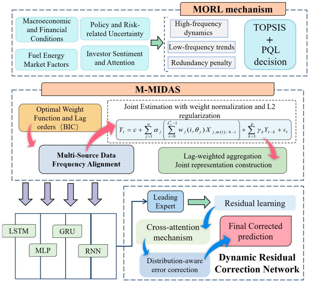
This study proposes a unified multi-step forecasting system with a sequential and hierarchical architecture, in which information is progressively refined through three interconnected modules, as illustrated in Figure 1. Different colored blocks denote distinct functional modules, and arrows indicate the data flow and interactions among components. First, the MORL-based mechanism of the feature selection module is employed to construct a compact yet informative subset from high-dimensional multisource inputs under multiple objectives, thereby providing a structured and noise-reduced representation for subsequent modeling. Second, based on the selected features, the M-MIDAS module captures heterogeneous temporal dependencies across mixed-frequency factors through a unified alignment mechanism, thereby generating the primary forecast. Finally, the LE-DRCN is introduced to further refine the predictions by modeling structured residual patterns via attention-based nonlinear mapping, enabling adaptive integration of complementary expert models.

Overall, the system follows a clear information flow from feature compression to mixed-frequency representation learning and subsequent residual correction, where each module addresses a specific limitation of existing methods while jointly contributing to a progressively refined forecasting process.

2.2. MORL Feature Selection Mechanism

This study formulates the multisource feature selection problem as a multi-objective sequential decision process and develops a MORL-based feature selection mechanism. Feature selection is modeled as an adaptive decision-making process that explores the feature space under multiple competing criteria, rather than as a static optimization problem [24]. By jointly considering high-frequency dynamics, low-frequency trends, and inter-feature redundancy, this mechanism enables structured feature extraction from high-dimensional multi-source data. For interval-valued forecasting, the MORL-based feature selection mechanism is conducted separately for the highest-price and lowest-price targets, so that the informative drivers of the upper and lower bounds can be identified in a target-specific manner.

Specifically, the feature selection process is formulated as an episodic multi-objective Markov decision process, defined by the tuple $\langle \mathcal{S},\mathcal{A},\mathcal{T},\mathcal{R},\gamma \rangle$, where $\mathcal{R}$ denotes a vector-valued reward function. In practical implementation, the state is encoded via a hashing-based compression mechanism to ensure tractability in high-dimensional spaces that is defined as $s_t=h({\mathcal{S}}_t)\hspace{0.17em}\mathrm{mod}\hspace{0.17em}{2}^{\min (p,20)}$. The action space $\mathcal{A}$ consists of discrete bit-flip operations that iteratively include or exclude individual features, thereby enabling structured exploration of the feature space. The transition function $\mathcal{P}$ is deterministic, ensuring that each action leads to a well-defined subsequent state, while the discount factor $\gamma$ controls the accumulation of future rewards.

A key innovation of the proposed system lies in the construction of a multi-view reward mechanism that explicitly characterizes the feature utility from a complementary perspective. Instead of scalar rewards, a three-dimensional reward vector is defined as:

$$R(s,a)={[r_1,r_2,r_3]}^T,$$

(1)

where each component is explicitly constructed as follows:

$$r_1={\displaystyle \frac{1}{\left|\mathcal{S}\right|}}{\displaystyle \sum _{i\in \mathcal{S}}{\tilde{S}}_i^H},\hspace{1em}{S}_i^H={\max }_{\mathcal{l}\in 0,\dots ,L}\mathrm{MI}(x_{i,t-\mathcal{l}},y_t^H)$$

(2)

$$r_2={\displaystyle \frac{1}{\left|\mathcal{S}\right|}}{\displaystyle \sum _{i\in \mathcal{S}}{\tilde{S}}_i^L},\hspace{1em}{\overline{x}}_{i,\tau }={\displaystyle \frac{1}{A}}{\displaystyle {\displaystyle \sum _{a=0}^{A-1}}{x}_{i,\tau A-a}},\hspace{1em}{S}_i^L=\mathrm{MI}({\overline{x}}_{i,\tau },y_{\tau }^L),$$

(3)

$$r_3=-{\max }_{i<j,,i,j\in \mathcal{S}}|{\rho }_s(x_i,x_j)|.$$

(4)

To ensure comparability across objectives, $S_i^H$ and $S_i^L$ are normalized using min–max scaling:

$${\tilde{S}}_i^H={\displaystyle \frac{S_i^H-\min S^H}{\max S^H-\min S^H+ϵ}},\hspace{1em}{\tilde{S}}_i^L={\displaystyle \frac{S_i^L-\min S^L}{\max S^L-\min S^L+ϵ}}.$$

(5)

Given the inherently conflicting nature of these objectives, no single feature subset can simultaneously optimize performance across all criteria. To address this issue, the proposed system adopts Pareto Q-learning for scalar-free multi-objective optimization [25]. Unlike conventional reinforcement learning methods that rely on scalarized rewards, Pareto Q-learning maintains a set of non-dominated Q-value vectors for each state–action pair, enabling the exploration of multiple optimal tradeoffs along the Pareto frontier. The action-value update rule is given by:

$$Q(s,a)=\mathrm{ND}\left({\displaystyle \underset{a^{\prime }}{\cup }\left\{R(s,a)+\gamma q^{\prime }|q^{\prime }\in Q(s^{\prime },a^{\prime })\right\}}\right),$$

(6)

where ND(·) denotes the Pareto non-dominated set operator. This update mechanism ensures that multiple competing feature-selection strategies are retained during the learning process, allowing the agent to approximate the true Pareto-optimal solution space in a data-driven manner [26].

In addition, action selection is guided by a hypervolume-based criterion to evaluate the quality of the Pareto sets:

$$\mathrm{Score}(a|s)=HV(\mathcal{Q}(s,a);r^{ref}).$$

(7)

After obtaining the Pareto-optimal feature subsets, we introduce a post-selection decision stage to identify a single deployable solution [27]. Specifically, the technique for order preference by similarity to ideal solution (TOPSIS) is applied to identify the most balanced solution. The positive ideal solution D⁺ and negative ideal solution D⁻ are constructed, and each candidate subset is evaluated based on its relative closeness to these solutions:

$$C_i={\displaystyle \frac{D_i^{-}}{D_i^{+}+D_i^{-}}}.$$

(8)

The subset with the maximum $C_i$ is selected as the final solution. As a result, the final feature subset is not determined by a single optimization criterion but by a structured compromise across multiple competing objectives, ensuring that the selected features jointly retain short-term volatility information and long-term trend characteristics while effectively controlling internal redundancy.

Because TOPSIS requires an explicit preference structure in the post-selection stage, the weight vector is designed to reflect the relative importance of the three objectives. Rather than being arbitrarily assigned, the weights are determined based on a preliminary sensitivity analysis. Specifically, several neighboring weight configurations were examined, and both the resulting feature rankings and downstream forecasting performance remained stable under moderate perturbations. Based on this robustness, the final settings, 0.4, 0.3, and 0.3, were therefore adopted as a balanced compromise, with a slightly larger weight assigned to the high-frequency relevance term to reflect the empirical importance of short-term shocks in carbon price dynamics, while the low-frequency trend term and redundancy penalty received equally moderate weights to preserve the temporal structure and reduce multicollinearity.

Notably, this weighting scheme does not affect the MORL optimization process itself. The proposed feature selection mechanism is implemented through Pareto Q-learning without scalarization, and the TOPSIS weights are introduced only at the final decision stage to select a single deployable solution from the Pareto set. The sensitivity analysis further confirms that the resulting feature subset remains robust under moderate perturbations of the weighting vector. The detailed procedure of the multi-objective feature selection mechanism is summarized in Algorithm 1.

Algorithm 1. MORL-Based Feature Selection with Pareto Q-learning
Input	$\mathrm{Initial} \mathrm{feature} \mathrm{pool} X,$  $\mathrm{target} \mathrm{variable} \mathrm{increment} \Delta Y,$  $\mathrm{maximum} \mathrm{training} \mathrm{epochs} E,$$\mathrm{TOPSIS} \mathrm{weights} W=\left[\mathrm{0.4,0.3,0.3}\right]$
Output	$\mathrm{Optimal} \mathrm{feature} \mathrm{subset} S^{\ast }$
Phase 1	Multi-Objective Optimization via Pareto Q-learning
1	$\mathrm{Initialize} \mathrm{Pareto} \text{Q-table} Q(s,a)$  $\mathrm{and} \mathrm{initial} \mathrm{state} s_0$
2	For e = 1 to E do
3	$\mathrm{Select} \mathrm{action} a_t$ $\mathrm{on} \mathrm{the} \mathrm{Pareto} \mathrm{front} \mathrm{using} ϵ$-greedy policy
4	$\mathrm{Execute} \mathrm{action} a_t,$ $\mathrm{and} \mathrm{observe} \mathrm{the} \mathrm{next} \mathrm{state} s_{t+1}$ and Evaluate multi-objective fitness
5	$\mathrm{Update} Q(s,a)$ using non-dominated sorting
6	End For
7	Extract all Pareto-optimal feature combinations, denoted as $P$
Phase 2	Compromise Decision-Making via TOPSIS
8	$\mathrm{Calculate} \mathrm{the} \mathrm{positive} \mathrm{ideal} \mathrm{distance} D^{+}$  $\mathrm{and} \mathrm{negative} \mathrm{ideal} \mathrm{distance} D^{-}$  $\mathrm{for} \mathrm{each} \mathrm{candidate} \mathrm{solution} \mathrm{in} P$
9	$\mathrm{Calculate} \mathrm{the} \mathrm{relative} \mathrm{closeness} \mathrm{score} C_i=D_i^{-}/(D_i^{+}+D_i^{-})$
10	Return$\mathrm{the} \mathrm{feature} \mathrm{set} \mathrm{with} \mathrm{the} \mathrm{highest} C_i$  $\mathrm{score} \mathrm{as} \mathrm{the} \mathrm{final} \mathrm{selection} S^{\ast }$

2.3. Multi-Source Mixed-Frequency Data Fusion via M-MIDAS

This section presents the M-MIDAS module, which integrates multi-source high-frequency information into a unified low-frequency representation. Unlike conventional MIDAS models that typically assume a single-input setting, the proposed module jointly processes heterogeneous high-frequency variables within a unified lag-weighted aggregation framework. By addressing heterogeneity, noise, and asynchronous timing through frequency alignment and lag-weighted aggregation, it enables effective information fusion while overcoming the single-input limitation of traditional mixed-frequency approaches. The specific procedures are detailed below.

2.3.1. Optimal Specification Identification

An independent specification search was conducted for each high-frequency explanatory variable to determine the optimal lag length and weighting structure. Specifically, the optimal parameter combination $({\widehat{K}}_i,{\widehat{\theta }}_i)$ was obtained by minimizing the information criterion in a source-specific regression as:

$$({\widehat{K}}_i,{\widehat{\theta }}_i)=\arg {\min }_{K_i,{\theta }_i}{\displaystyle \sum _{t=1}^T{\left(y_t-{\alpha }_i-{\displaystyle {\displaystyle \sum _{j=1}^p}{\gamma }_{ij}}{y}_{t-j}-{\beta }_i{\displaystyle {\displaystyle \sum _{k=0}^{K_i-1}}{w}_i}(k;{\theta }_i)X_{i,\mathrm{map}(t)-h-k}\right)}^2},$$

(9)

where $K_i$ denotes the optimal lag length and ${\theta }_i$ represents the parameters of weighting function $w_i(\cdot )$. The candidate weighting functions include Beta, BetaNN, exponential Almon, Almon lag, step function, unrestricted MIDAS, and Legendre polynomials. This stage ensures that variable-specific temporal dynamics are flexibly captured.

2.3.2. Multi-Source Frequency Alignment

The core component of the proposed system is a systematic multisource frequency-alignment procedure that transforms heterogeneous high-frequency variables into a unified feature matrix suitable for low-frequency regression. This procedure plays a central role in mitigating the frequency mismatch among diverse information sources. Instead of processing each high-frequency variable independently, it constructs a structured representation that preserves the joint dynamics across multiple information streams.

Let $Y_t$ denote a low-frequency observation ending at date $d_t$, and let $X$ represent the set of $n$ high-frequency time series. At any high-frequency time index $\tau$, the system state is defined as $X_{\tau }={[X_{1,\tau },\dots ,X_{n,\tau }]}^{\prime }$, which captures the synchronized observations across all variables at time $\tau$. To establish a consistent mapping between low-frequency targets and high-frequency information, a horizon parameter $h$ is introduced to define the real-time information set. Specifically, let $loc$ denote the high-frequency index corresponding to the low-frequency endpoint $d_t$. The effective information alignment point is then determined as:

$$alig{n}_t=loc-h,$$

(10)

which identifies the most recent high-frequency state available for predicting $Y_t$, thereby ensuring that no future information is incorporated into the modeling process.

This formulation guarantees that the model relies exclusively on observations that precede the forecasting horizon, thereby preventing the leakage of future information. Let the optimal lag configuration be denoted as $L=[L_1,\dots ,L_n]$. To ensure consistency across variables, a common lag length is introduced by defining the system-wide upper bound $L_{max}=\max (L)$. This upper bound defines the maximum historical window required to effectively represent high-frequency inputs. Based on this unified lag scheme, the feature representation $Z_t$ is obtained by jointly sampling all variables in a temporally aligned manner:

$$Z_{t,(i\cdot n+j)}=\left\{\begin{array}{ll}{X}_{j,(align-i)}\hfill & \mathrm{if} i<L_j^{\ast }\hfill \\ 0\hfill & \mathrm{if} i\ge L_j^{\ast }\hfill \end{array}\right..$$

(11)

This process can be equivalently expressed as a concatenation of historical system states:

$$Z_t=\left[\underset{\mathrm{State} \mathrm{at} \mathrm{Lag} 0}{\underbrace{{\tilde{X}}_{a_t^{align}}}},\underset{\mathrm{State} \mathrm{at} \mathrm{Lag} 1}{\underbrace{{\tilde{X}}_{a_t^{align}-1}}},\dots ,\underset{\mathrm{State} \mathrm{at} \mathrm{Lag} L_{max}-1}{\underbrace{{\tilde{X}}_{a_t^{align}-L_{max}+1}}}\right].$$

(12)

The final design matrix was obtained by stacking $Z_t$ across all admissible low-frequency time points. This representation converts heterogeneous high-frequency signals into a coherent input format, while maintaining temporal dependencies and preserving the interactions among variables across different sources.

2.3.3. Joint Lag-Weighted Aggregation

Building on the aligned representation, a lag-weighted aggregation scheme is applied to extract low-frequency M-MIDAS factors. For each feature $x_i$, the corresponding factor is defined as:

$$Zi,t={\displaystyle \sum _{k=0}^{Li}\omega }\left(ki;\theta i\right)xi,t-k,$$

(13)

where $L_i$ and $\omega (k;{\theta }_i)$ are determined at the specification stage. Unlike conventional approaches that treat each variable independently, the proposed system integrates all extracted factors into a unified representation:

$$Z_t=[Z_{1,t},Z_{2,t},\dots ,Z_{n,t}].$$

(14)

This joint formulation ensures the simultaneous incorporation of multiple information sources, thereby enabling the model to capture individual temporal dependencies and cross-variable interactions.

Following this procedure, the M-MIDAS module converts raw high-frequency inputs into a structured and temporally aligned low-frequency feature space. This unified representation reduces noise and redundancy while overcoming the single-input limitation of conventional MIDAS models, thereby enabling the coordinated integration of multiple heterogeneous information streams. Consequently, it provides a robust and information-rich foundation for subsequent interval-valued forecasting tasks.

2.4. Deep Learning Base Predictors

As established in the previous section, the M-MIDAS module enables the transformation of heterogeneous mixed-frequency inputs into a structured low-frequency feature matrix. Using this representation, the learning objective is further reformulated to improve robustness under nonstationary carbon price dynamics and align with multistep forecasting.

Instead of directly predicting the absolute price levels, the model was designed to estimate future variations in the highest and lowest prices. This reformulation shifts the focus from level estimation to dynamic change modeling, thereby reducing scale dependency and enhancing sensitivity to evolving market conditions [28]. Furthermore, it naturally supports a direct multistep forecasting strategy in which each forecasting horizon is treated as an independent learning task, effectively avoiding recursive error accumulation. Specifically, given the original price series, the H-step prediction target is defined as:

$$y_{t+H} = P_{t+H} - P_t.$$

(15)

Under this transformation, the processed M-MIDAS features are mapped to increment-based targets through a set of deep learning models, including a multi-layer perceptron (MLP), recurrent neural network (RNN), LSTM, and gated recurrent unit (GRU). The details of these models are described below.

2.4.1. MLP

The MLP serves as the foundational feedforward neural network in our system. This network is highly effective for approximating complex nonlinear functions without assuming a temporal sequence [29]. For a given input vector ${{\rm Z}}_t$, the data are propagated forward through one or more hidden layers. The transformation at a specific hidden layer can be formulated as:

$$h_t=\sigma (W_h\hspace{0.33em}{Z}_t+b_h),$$

(16)

where $W_h$ and $b_h$ represent the weight matrix and bias vector of the hidden layer, respectively, and $\sigma \left(\cdot \right)$ denotes a nonlinear activation function. The final output layer directly maps the extracted abstract representations to the highest and lowest predicted prices. In this study, the MLP provides a robust baseline for capturing the instantaneous, cross-variable synergistic effects among M-MIDAS factors.

2.4.2. RNN

Unlike an MLP, an RNN is inherently designed to process sequential data by introducing a memory mechanism via a hidden state [30]. This allows the network to maintain information about previous time steps, making it suitable for time-series forecasting. At time step $t$, the RNN updates its hidden state $h_t$ based on both the current M-MIDAS feature input ${\mathrm{Z}}_t$ and the hidden state from the previous step $h_{t-1}$ as:

$$h_t=\tanh (W_z{\mathrm{Z}}_t+W_r{h}_{t-1}+b).$$

(17)

where $W_z$ and $W_r$ are the weight matrices of the input and recurrent connections, respectively, and $b$ is the bias. While RNNs conceptually capture temporal dynamics, they frequently suffer from vanishing or exploding gradients when processing long sequences, which limits their ability to capture the long-term macroeconomic trends that affect carbon prices.

2.4.3. LSTM

To overcome the limitations of the standard RNN, the LSTM network introduces a complex memory cell structure regulated by three distinct gating mechanisms: the forget gate, input gate, and output gate [31]. This architecture enables the model to selectively retain relevant long-term information while discarding irrelevant short-term noise. The operations within an LSTM cell at time $t$ are governed by the following equations:

$$i_t=\sigma (W_i\cdot [Z_t,h_{t-1}]+b_i),$$

(18)

$$t=\sigma (W_i\cdot [Z_t,h_{t-1}]+b_i),$$

(19)

$$C_t=tanh(W_C\cdot [Z_t,h_{t-1}]+b_C),$$

(20)

$$o_t=\sigma (W_o\cdot [Z_t,h_{t-1}]+b_o),$$

(21)

$$h_t=o_t\odot \tanh (C_t),$$

(22)

where $f_t$, $i_t$, and $o_t$ represent the activation vectors of the forget, input, and output gates, respectively. $C_t$ is a cell state that acts as a long-term memory conveyor and $\odot$ denotes element-wise multiplication [32]. By utilizing this sophisticated gating logic, LSTM provides a superior ability to model the nonlinear, long-memory characteristics of interval-valued carbon prices.

2.4.4. GRU

The GRU is a highly efficient variant of the LSTM architecture. It simplifies structural complexity by merging the cell and hidden states and by combining the forget and input gates into a single update gate [33]. This streamlined design reduces the number of trainable parameters, thereby mitigating the risk of overfitting, while maintaining comparable performance in capturing temporal dependencies. The updating process in a GRU is defined as

$$z_t=\sigma (W_z\cdot [Z_t,h_{t-1}]+b_z),$$

(23)

$$r_t=\sigma (W_r\cdot [Z_t,h_{t-1}]+b_r),$$

(24)

$${\tilde{h}}_t=\tanh (W_h\cdot [Z_t,(r_t\odot h_{t-1})]+b_h),$$

(25)

$$h_t=(1-Z_t)\odot h_{t-1}+Z_t\odot h_t.$$

(26)

On the basis of these gating decisions, a candidate hidden state ${\tilde{h}}_t$ is first constructed by selectively incorporating relevant historical signals. The final hidden state $h_t$ is then obtained through a weighted integration of the previous hidden state and candidate state, enabling the model to dynamically balance memory preservation and information updating over time [34].

2.5. LE-DRCN

Although the M-MIDAS module generates temporally aligned representations and preliminary forecasts from heterogeneous base predictors, effectively synthesizing these outputs into a reliable final prediction remains a challenge. In particular, forecasting errors exhibit systematic state-dependent patterns rather than pure randomness, making static ensemble strategies insufficient. To address this issue, we propose LE-DRCN, which first identifies the dominant price dynamics through the most proficient expert and then employs a cross-expert attention-based residual correction mechanism to dynamically adjust structured residual errors.

Within this system, a pool of candidate expert models is first constructed, and an optimal leading expert selection strategy is proposed to identify the most reliable predictor. In the main implementation, the leading expert is selected from the candidate models according to the minimum training root mean square error (RMSE). The RMSE is adopted because it is consistent with the squared-error optimization objective and is sensitive to large deviations, which is particularly relevant in carbon price dynamics. To further enhance the reliability of expert selection, we perform a rolling-window time-series validation procedure, in which candidate experts are repeatedly evaluated over sequential validation folds to assess their stability under temporal variation. The cross-validated performance is computed as follows:

$$i^{\ast }=\arg {\min }_{i\in 1,\dots ,M}{\displaystyle \frac{1}{F}}{\displaystyle \sum _{f=1}^{F}R}MS{E}_i^{(f)},$$

(27)

where $M$ is the number of candidate experts and $F$ denotes the number of validation folds. Under nonstationary market conditions, the model further adopts a rolling training strategy, allowing the leading expert to be updated as new observations arrive. This design avoids persistent reliance on a single in-sample optimal model and improves adaptability to evolving carbon market regimes. The leading expert is then used to generate the primary forecast:

$${\widehat{y}}_t^{(base)}=f_{i\ast }(x_t),$$

(28)

where $e_t$ denotes the residual at time step $t$, $y_t$ is the true value, and $y_{leader,t}$ is the baseline prediction provided by the leading expert.

To further improve predictive performance, a cross-expert attention-based residual attention mechanism was introduced to model residual dependencies by leveraging the collective outputs of all candidate experts. At each time step $t$, the predictions of all experts are organized into a vector ${\widehat{y}}_t=[{\widehat{y}}_{1,t},\dots ,{\widehat{y}}_{M,t}]$ that characterizes the distribution of the model predictions across the expert pool. To enable effective information interaction within the attention mechanism, each scalar prediction is projected into a shared latent space through a learnable transformation:

$$h_{i,t}=W_p{\widehat{y}}_{i,t},$$

(29)

where ${\widehat{y}}_{i,t}$ denotes the prediction of the i-th expert at time step $t$, $W_p\in {ℝ}^{d\mathrm{model}\times 1}$ is a learnable projection matrix, and $h_{i,t}\in {ℝ}^{d\mathrm{model}}$ is the embedded representation. These projected features are then stacked to form the key and value matrices $K_t=V_t=\left[h_{1,t},\dots ,h_{M,t}\right]$, where $K_t,V_t\in {ℝ}^{M\times d_{\mathrm{model}}}$.

A central component of this design is the introduction of a learnable global query vector $Q_{\mathrm{global}}$, which is independent of the input sequence and is optimized during training. Unlike conventional attention mechanisms in which queries are derived from local inputs, this global query acts as a task-specific probe that extracts residual-relevant information from the prediction distribution [35]. The interaction between the global query and expert representations is modeled through scaled dot-product attention, yielding a context vector defined as:

$$c_t=\mathrm{Softmax}\left({\displaystyle \frac{Q_{\mathrm{global}}{K}_t^{\top }}{\sqrt{d_{\mathrm{model}}}}}\right)V_t,$$

(30)

where $Q_{\mathrm{global}}\in {ℝ}^{1\times d_{\mathrm{model}}}$ is the learnable global query vector, $K_t\in {ℝ}^{M\times d_{\mathrm{model}}}$ and $V_t\in {ℝ}^{M\times d_{\mathrm{model}}}$ denote the key and value matrices constructed from the projected expert features, respectively, $d_{\mathrm{model}}$ is the dimensionality of the latent space, and $c_t\in {ℝ}^{1\times d_{\mathrm{model}}}$ is the resulting context vector that aggregates information from all experts. Through this operation, the model dynamically evaluates the relevance of each expert and aggregates complementary information in a data-driven manner.

This mechanism enables the model to explicitly capture the state-dependent nature of predictive errors by learning the dynamic relationship between the collective forecast distributions and baseline residuals [36]. The resulting context vector is then passed through a feedforward network to estimate the residual correction:

$${\widehat{e}}_t=\mathrm{FFN}(c_t),$$

(31)

where ${\widehat{e}}_t$ denotes the predicted residual. This design enables distribution-aware error refinement, in which the correction process is guided by the prediction distribution of all experts, rather than static weighting rules [37].

Finally, the overall prediction is obtained by combining the leading expert forecast with the estimated residual, formulated as follows:

$${\widehat{y}}_{\mathrm{final},t}=y_{leader,t}+{\widehat{e}}_t.$$

(32)

The proposed LE-DRCN establishes a principled connection between ensemble learning and residual modeling, providing a unified and interpretable module for multistep interval-valued forecasting in complex environments. Algorithm 2 outlines the complete two-stage training and prediction pipeline of the proposed LE-DRCN module.

Algorithm 2. LE-DRCN Residual Correction Network
Input	Sub-model expert prediction matrix $P\in R^{N\times M},$ actual price increment $\Delta Y,$ learning rate $\eta$
Output	Final corrected prediction $Y_{final}$
Stage 1	Leading Expert Anchoring
1	For expert m = 1 to M do
2	Initialize rolling window: training size $Ttrain,$ validation size $Tval$
3	For k = 1 to K do
4	Extract training set $Dtrain\left(k\right)=\left[t_k:t_k+Ttrain\right]$
6	Extract validation set $Dval\left(k\right)=\left[t_k+Ttrain:t_k+Ttrain+Tval\right]$
7	Evaluate expert m on $Dval\left(k\right)$ and record error metrics
8	End For
9	Aggregate validation errors: $Erro{r}_m={\displaystyle \frac{1}{K}}{\sum }_{k=1}^K=RMS{E}_m^{(k)}$
10	End For
11	Select the leading expert
Stage 2	Residual Attention Correction
12	For epoch = 1 to $Epochs$ do
13	For batch in DataLoader do
14	Linear projection into feature space: $K,V,Q=Linear\left(P\right)$
15	Calculate expert cross-attention weights $\hspace{0.33em}A=Softmax(Q{K}^T/\sqrt{d_{model}})$
16	Dynamically aggregate correction terms $\widehat{E}=Attentio{n}_{weights}\cdot P$
17	Compute the Mean Squared Error (MSE) loss; perform backpropagation; and update model parameters using the Adam optimizer.
18	End For
19	Return$\hspace{0.33em}{Y}_{final}=Y_{base}+\widehat{E}$

3. Data and Experimental Setup

This section presents the empirical framework used to evaluate the proposed multi-source mixed-frequency interval-valued carbon price forecasting system. The experimental design integrates data construction, model specification, and performance evaluation into a unified pipeline, ensuring consistency between methodological development and empirical validation. Specifically, the following subsections describe the dataset and variable construction, benchmark models, model training strategy, and evaluation metrics.

3.1. Data Description

This study empirically investigates the effectiveness of the proposed system using the China Emission Allowance (CEA) market. CEA carbon price data and all influencing factors are collected from authoritative financial data platforms, primarily the Wind database and Investing.com (https://www.investing.com/), to ensure data consistency and reliability. In addition to market-based financial and macroeconomic variables, the dataset further introduces external information indicators capturing policy and macroeconomic uncertainty, as well as internet-based measures of market attention, sentiment and attention indicators derived from internet-based information and search behavior. The sample period spans 16 July 2021 (the date of the official launch of China’s national carbon market) to 30 May 2025. This sample period covers both the initial establishment and subsequent development of China’s national carbon market, including gradual policy refinement, mechanism adjustment, and sectoral expansion.

3.1.1. Target Variable

After the CEA carbon price data were collected from the Wind database and Investing.com (https://www.investing.com/), the daily price series were further transformed into weekly interval targets to match the interval-valued forecasting objective, where the highest and lowest prices within each week were used to represent intra-week price fluctuations. Specifically, the weekly interval-valued target was defined as:

$$P_t^H=\max \left\{p_{(i,t)}^{high}\right\},i\in \{1,2,\dots ,N_t\}$$

(33)

$$P_t^L=\min \left\{p_{(i,t)}^{low}\right\},i\in \{1,2,\dots ,N_t\}$$

(34)

where $p_{(i,t)}^{high}$ and $p_{(i,t)}^{low}$ denote the highest and lowest daily prices on the $i-th$ trading day of week $t$, respectively, and $N_t$ is the total number of actual trading days in that specific week.

3.1.2. Multi-Source Influencing Factors

Carbon price formation in an ETS is driven by multiple interconnected economic transmission channels rather than isolated variables [38]. From a systems perspective, price dynamics emerge through four primary mechanisms: macro-financial transmission, policy and uncertainty shocks, energy market cost transmission, and investor sentiment-driven behavioral responses [39]. Guided by this mechanism-driven framework, 47 exogenous variables were selected to comprehensively represent these four transmission pathways. Each group of variables was designed to capture one distinct mechanism through which external information is incorporated into carbon price dynamics. A detailed definition of all factors is provided below.

(1) Macroeconomic and Financial Conditions

Macroeconomic and financial market conditions influence carbon prices through macro-financial transmission channels, reflecting changes in economic activity, capital flows, and investor risk sentiments. Equity indices capture the overall financial market performance and risk appetite, whereas exchange rates reflect cross-border capital movement and currency risk. Commodity prices, including gold and energy-related assets, further transmit global liquidity conditions and cost-side shocks to the carbon markets. Specifically, variables such as the CSI 300, ChiNext Index, FTSE China Index, S&P 500, and EURO STOXX indices are employed to represent domestic and international equity markets. Exchange rates capture currency dynamics, while gold prices and the US Dollar Index serve as proxies for global liquidity and safe-haven demand. In addition, crude oil and natural gas futures are included to reflect the energy-financial linkages that affect carbon pricing mechanisms.

(2) Policy and Risk-related Uncertainties

Carbon markets are highly sensitive to policy interventions and external shocks, which makes uncertainty a critical factor in price formation. Macroeconomic policy uncertainty, geopolitical tensions, and climate-related risks can significantly influence market expectations and trading behavior [40]. To account for these effects, this study incorporated multiple uncertainty indicators, including Economic Policy Uncertainty (EPU) indices for China, Europe, and the global market, as well as broader measures such as sustainability uncertainty and geopolitical risk indices. Furthermore, transition and physical climate risk indices were included to capture the long-term uncertainties associated with climate policy and environmental changes.

(3) Fuel Energy Market Factors

Energy prices are widely recognized as one of the most direct drivers of carbon price fluctuations because they influence the cost structure of electricity generation and relative competitiveness of different energy sources. Variations in fossil fuel prices can alter energy consumption patterns and emissions levels, thereby affecting the supply–demand balance in carbon markets [41]. This dimension incorporates key energy price indicators, including natural gas prices, crude oil benchmarks, such as Brent and West Texas Intermediate (WTI) futures, coal prices, and biofuel indices. In addition, clean energy-related financial instruments such as global clean energy exchange-traded funds (ETFs) are included as proxies for capital market expectations regarding energy transition and its potential impact on carbon pricing dynamics.

(4) Investor Sentiment and Attention

Beyond traditional structured variables, recent studies highlight the increasing importance of behavioral factors in financial markets. Investor attention and sentiment, which are often derived from big data sources, can influence trading intensity, market expectations, and price volatility [42]. In this study, a set of attention-based indicators was employed to capture these behavioral dynamics, including attention to carbon prices, supply-demand conditions, and carbon trading activities, as well as attention to energy policies and geopolitical risks. Additionally, extreme weather indices and attention to extreme events are incorporated to reflect the impact of climate-related shocks and public awareness on market behavior [43].

Following the identification of the multisource feature variables,

Table 1. Description of variables.

Category	Symbol	Full Name
Target Variables	CEA_H	Weekly Highest Price of CEA
	CEA_L	Weekly lowest Price of CEA
	CEA_D	Daily Price of CEA
Uncertainty Indicators	CEPU	China Economic Policy Uncertainty
	GEPU	Global Economic Policy Uncertainty
	GSU	Global Sustainability Uncertainty
	GPR	Geopolitical Risk Index
	GPR_E	Geopolitical Risk Events
	GPR_T	Geopolitical Risk Threats
	TRI	Transition Risk Index
	PRI	Physical Risk Index
Macroeconomic and Financial Markets	BCI	Beautiful China Index
	CNT	ChiNext Index
	CSI300	China Securities Index 300
	FTSE_CN	Financial Times Stock Exchange China Index
	HCI	Healthy China Index
	SP500	Standard & Poor’s 500 Index
	DJ_EU	Dow Jones Europe
	STOXX50	EURO STOXX 50
	STOXX600	EURO STOXX 600
	MSCI_EU	Morgan Stanley Capital International Europe
	Gold_CNY	Spot Gold (CNY)
	Gold_EUR	Spot Gold (EUR)
	DXY	US Dollar Index
	USDCNY	USD/CNY Exchange Rate
	USDEUR	USD/EUR Exchange Rate
	MSCI_NZ	MSCI New Zealand
	NZX50	S&P/NZX 50 Index
	Gold_NZD	Spot Gold (NZD)
	USDNZD	USD/NZD Exchange Rate
	WTI	WTI Crude Oil Futures
	Brent	Brent Crude Oil Futures
	NatGas_US	NYMEX Natural Gas
Energy Markets	NatGas_UK	UK NBP Natural Gas
	Coal	Rotterdam Coal Futures
	LCI_CN	China Low-Carbon Index
	NEI	New Energy Index
	SCCE	Solactive China Clean Energy
	Biofuels	S&P GSCI Biofuels Index
	GCE-BR	iShares Global Clean Energy ETF
	WCE	Invesco WilderHill Clean Energy
	GCE-IV	Invesco Global Clean Energy ETF
	LCE	VanEck Low Carbon Energy ETF
Investor Sentiment	S_Trade	Baidu Index: Trading
	S_Policy	Baidu Index: Energy Policy
	S_Price	Baidu Index: Energy Price
	S_Event	Baidu Index: Extreme Events
	S_Geo	Baidu Index: Geopolitics
	S_Supply	Baidu Index: Supply & Demand
	S_Weather	Baidu Index: Extreme Weather

summarizes the detailed definitions and corresponding categories of all 47 exogenous factors and the multifrequency carbon price targets.

3.2. Benchmark Models

To evaluate the effectiveness of the proposed system, the deep learning base predictors used in this system, i.e., LSTM, GRU, RNN and MLP, were selected as benchmark models: LSTM and GRU are widely used recurrent neural networks capable of capturing temporal dependencies in sequential data; RNN serves as a baseline for recurrent network-based sequential modeling; MLP models nonlinear relationships between exogenous variables and carbon prices without explicit temporal memory. All benchmark models were implemented using the same input configuration, with identical feature sets and forecasting horizons to ensure a fair comparison. The hyperparameter search spaces for all benchmark models are summarized in

Table 2. Hyperparameter search spaces of benchmark models.

Model	Seq. Length	Hidden Layer Size	Number of Layers	Dropout	Learning Rate	Batch Size	Weight Decay
GRU	[3, 5]	{16, 32, 64}	{1, 2, 3}	{0.2, 0.3, 0.5}	{1 × 10−4, 5 × 10−4, 1 × 10−3}	{16, 32, 64}	{1 × 10−5, 1 × 10−4}
LSTM	[3, 5]	{16, 32, 64}	{1, 2, 3}	{0.3, 0.4, 0.5}	{1 × 10−4, 5 × 10−4, 1 × 10−3}	{16, 32, 64}	{1 × 10−5, 1 × 10−4}
RNN	[3, 5]	{16, 32, 64}	{1, 2, 3}	{0.2, 0.3, 0.5}	{1 × 10−4, 5 × 10−4, 1 × 10−3}	{16, 32, 64}	{1 × 10−5, 1 × 10−4}
MLP	[3, 5]	{32, 64, 128}	{1, 2, 3}	{0.3, 0.4, 0.5}	{1 × 10−4, 5 × 10−4, 1 × 10−3}	{16, 32, 64}	{1 × 10−5, 1 × 10−4}
LE-DRCN	[3, 5]	{8, 16, 32, 64}	{1, 2, 3}	{0.3, 0.4, 0.5}	{1 × 10−4, 5 × 10−4, 1 × 10−3}	{8, 16, 32}	{1 × 10−5, 1 × 10−4}

. A grid search strategy was employed to ensure a fair comparison across all competing methods, where the optimal configuration was selected based on the validation performance on the training set.

3.3. Model Specification

To preserve temporal dependence and prevent information leakage, the processed dataset was organized in chronological order and divided into training and test sets using a ratio of 7:3. Within the training sample, a three-fold rolling-window cross-validation scheme was implemented to improve robustness during model training and hyperparameter selection under temporal distribution shifts.

Data preprocessing. Z-score normalization was applied to eliminate scale differences across variables.

Inputs. The proposed system utilizes historical carbon prices, influencing factors, and categorical variables as input information. These variables encode temporal dependencies from past observations and are subsequently processed through the M-MIDAS module to generate unified representations for forecasting.

Outputs. The forecasting task is formulated as a multi-step interval-valued prediction problem with horizons H = 1, 2, …, 5, where each step corresponds to forecasts of the lowest and highest carbon prices over the next one to five weeks, respectively.

Training strategy. Given the nonstationary nature of carbon markets, the proposed system adopts a rolling-window training strategy, under which the relationship between predictors and carbon prices is treated as locally stable within each training window. This design enables tractable modeling under evolving market conditions. In addition, a dynamic expert selection mechanism was introduced to improve adaptability over time.

3.4. Evaluation Metrics

A variety of performance measures have been developed in interval-valued time series forecasting to evaluate prediction quality from multiple perspectives, including boundary accuracy, interval-valued stability, and dynamic consistency [44,45]. These studies highlight the necessity of jointly assessing both deviation-based and variability-based characteristics when evaluating interval-valued forecasts. Motivated by this general evaluation paradigm, we adopt a widely used set of metrics, including interval mean absolute percentage error (IMAPE), interval RMSE (IRMSE), interval mean squared prediction error (IMSPE), Theil’s uncertainty index (UI), interval mean deviation error (IMDE), and interval adjusted relative variance (IARV), to comprehensively assess forecasting performance. Let $L_t$ and $U_t$ be the actual lowest and highest prices at time $t$, and let ${\widehat{L}}_t$ and ${\widehat{U}}_t$ be their respective forecasts. The detailed interval-valued evaluation metrics are reported in

Table 3. Description of the evaluation metrics.

Metric	Definition	Equation
IMAPE	Interval mean absolute percentage error	$\mathrm{IMAPE}={\displaystyle \frac{1}{2n}}{\displaystyle \sum _{t=1}^T\left(\left|\frac{L_t-{\widehat{L}}_t}{L_t}\right|+\left|\frac{U_t-{\widehat{U}}_t}{U_t}\right|\right)}$
IRMSE	Interval root mean squared error	$\mathrm{IRMSE}={\displaystyle \frac{1}{2}}\left(\sqrt{{\displaystyle \frac{1}{n}}{\displaystyle \sum _{t=1}^n{(L_t-{\widehat{L}}_t)}^2}}+\sqrt{{\displaystyle \frac{1}{n}}{\displaystyle \sum _{t=1}^n{(U_t-{\widehat{U}}_t)}^2}}\right)$
IMSPE	Interval mean squared percentage error	$\mathrm{IMSPE}={\displaystyle \frac{1}{2n}}{\displaystyle \sum _{t=1}^n\left({\left(\frac{L_t-{\widehat{L}}_t}{L_t}\right)}^2+{\left(\frac{U_t-{\widehat{U}}_t}{U_t}\right)}^2\right)}$
UI	Theil’s uncertainty index	$\mathrm{UI}=\sqrt{{\displaystyle \frac{{\displaystyle \sum _{t=2}^n\left[{({\widehat{L}}_t-L_t)}^2+{({\widehat{U}}_t-U_t)}^2\right]}}{{\displaystyle \sum _{t=2}^n\left[{(L_t-L_{t-1})}^2+{(U_t-U_{t-1})}^2\right]}}}}$
IMDE	Interval mean deviation error	$\mathrm{IMDE}={\displaystyle \frac{1}{2n}}{\displaystyle \sum _{t=1}^n\left(\left|(U_t-L_t)-({\widehat{U}}_t-{\widehat{L}}_t)\right|+\left|\frac{U_t+L_t}{2}-\frac{{\widehat{U}}_t+{\widehat{L}}_t}{2}\right|\right)}$
IARV	Interval adjusted relative variance	$\mathrm{IARV}={\displaystyle \frac{{\displaystyle \sum _{t=2}^n((}{L}_t-{\widehat{L}}_t{)}^2+{(U_t-{\widehat{U}}_t)}^2)}{{\displaystyle \sum _{t=2}^n((}{L}_t-L_{t-1}{)}^2+{(U_t-U_{t-1})}^2)}}$

.

4. Results and Discussion

To comprehensively evaluate the forecasting performance and effectiveness of the proposed multi-step interval-valued forecasting system, this section presents a series of comparative analyses. The detailed analysis was organized around five research questions:

RQ1: Can the proposed MORL mechanism effectively achieve a balanced selection of informative features from high-dimensional multisource data?

RQ2: Does the proposed M-MIDAS module enhance predictive performance by transforming raw multisource high-frequency inputs into a unified low-frequency representation, compared with both traditional MIDAS approaches and models without frequency alignment?

RQ3: Does the proposed integrated system, which combines M-MIDAS-based representation and ensemble learning, achieve superior accuracy and stability in multistep interval-valued forecasting compared with individual base predictors operating on raw or non-aligned inputs?

RQ4: Does the proposed LE-DRCN ensemble module outperform existing ensemble approaches in terms of predictive accuracy and stability in multistep interval-valued forecasting?

RQ5: What do the component-wise ablation results and interpretability analysis reveal about the underlying mechanisms of the proposed system across different forecasting horizons?

4.1. Results of the MORL Mechanism

This section presents the results for RQ1, which is whether the proposed MORL mechanism effectively balances the high-frequency dynamics, low-frequency trends, and inter-feature redundancy, resulting in a compact and informative subset of predictors. As shown in

Table 4. Results of feature selection.

Symbol	Full Name	Category	H-Score	L-Score
USDCNY	USD/CNY Exchange Rate	Macro/Fin	1.2567	1.0021
STOXX50	EURO STOXX 50	Macro/Fin	1.2545	0.9085
S_Event	Extreme Events Attention Index	Sentiment	1.0656	0.8484
NatGas_UK	UK NBP Natural Gas	Energy	0.9200	0.5762
USDNZD	USD/NZD Exchange Rate	Macro/Fin	0.9155	0.5176
NZX50	S&P/NZX 50 Index	Macro/Fin	0.8555	0.6006
S_Trade	Trading Attention Index	Sentiment	0.8033	0.6277
Brent	Brent Crude Oil Futures	Energy	0.7500	0.4470

Note: The H-score denotes mutual information with daily price dynamics, whereas the L-score represents mutual information with weekly trend components.

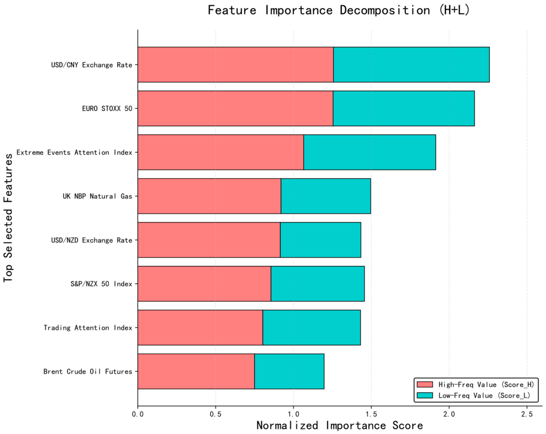
, the selected features span three key dimensions: macro-financial conditions, energy markets, and investor sentiment. Figure 2 illustrates the normalized importance scores of the top selected variables, explicitly decomposed into their high-frequency and low-frequency contributions. The results confirm that carbon price formation is jointly driven by economic fundamentals, cost-side factors, and behavioral responses rather than by any single information source. Importantly, these features correspond to distinct economic transmission channels, forming a coherent mechanism-based explanatory framework.

First, from a macro-financial perspective, exchange rates and international equity indices exhibit strong explanatory power. In particular, USDCNY and EURO STOXX 50 outperform other features in capturing short-term fluctuations, indicating that both domestic macroeconomic expectations and international market signals play a critical role in shaping carbon price dynamics. Second, the energy-related variables also play a critical role in this process. Energy prices directly affect marginal abatement costs faced by regulated firms. Increases in natural gas and crude oil prices alter energy substitution patterns and emissions intensity, thereby influencing carbon allowance demand and prices. Natural gas prices in the United Kingdom and Brent crude oil were identified as key drivers, highlighting the energy-to-carbon price transmission mechanism. Finally, the investor sentiment variables capture behavioral responses to market uncertainty. Search-based attention indicators reflect information diffusion and expectation-formation. For example, attention to extreme events is highly sensitive to policies and climate shocks, which often trigger short-term volatility. Meanwhile, trading-related attention serves as a proxy for market participation and liquidity, thus influencing price discovery dynamics.

4.2. Effectiveness of the M-MIDAS Module

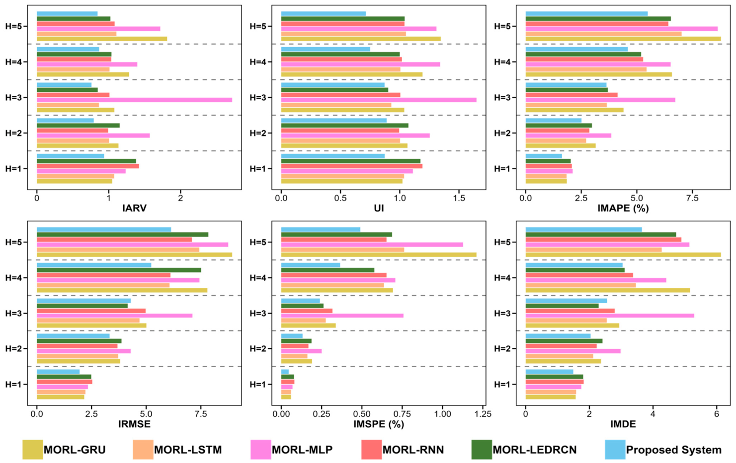
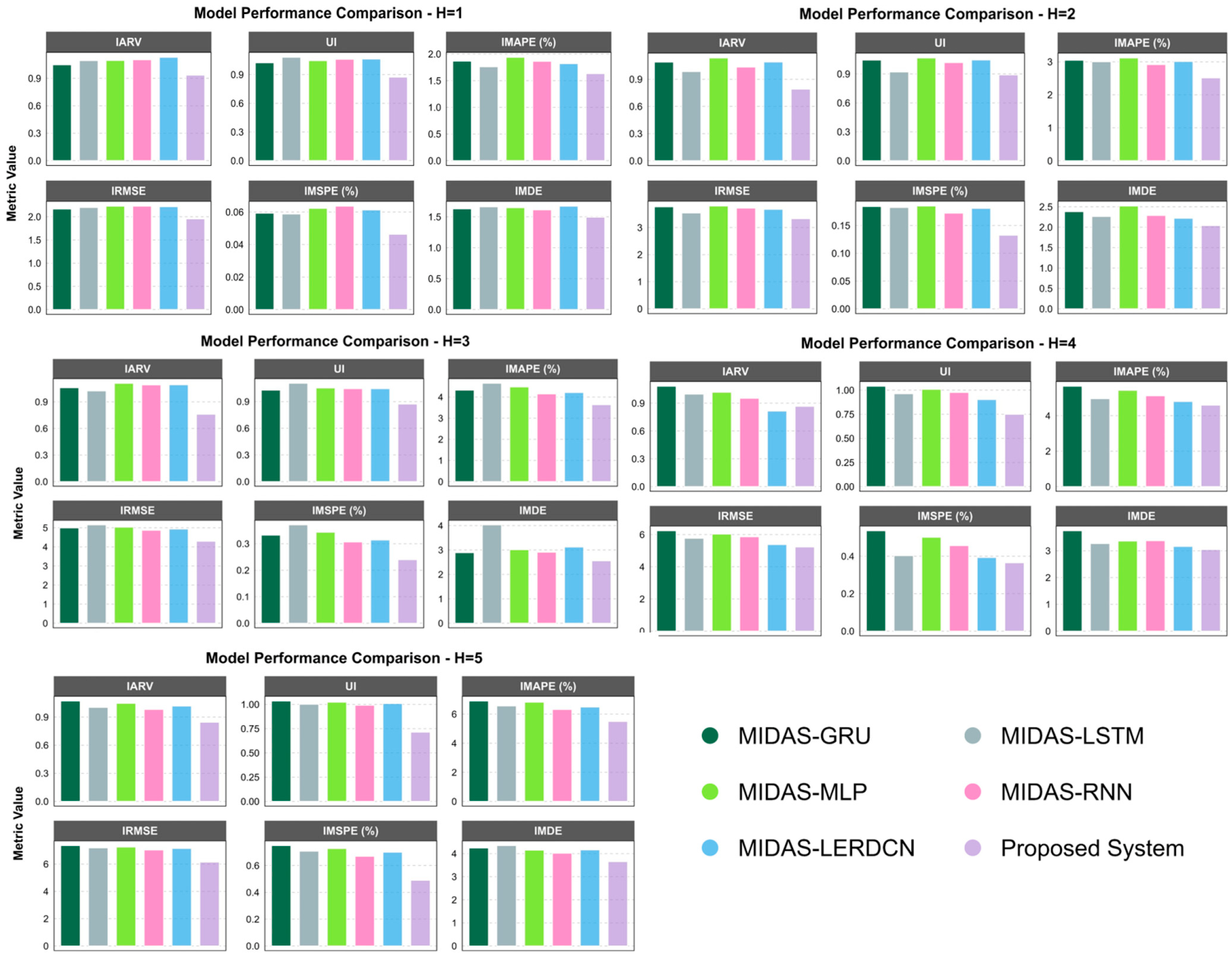
To address RQ2, this subsection presents the results evaluating whether the proposed M-MIDAS module improves predictive performance by transforming raw multi-source high-frequency inputs into a unified low-frequency representation. Specifically, an analysis was conducted that compared models without the M-MIDAS module with models incorporating the traditional MIDAS framework to assess the effectiveness of jointly modeling heterogeneous information sources. The comparative results across multiple forecasting horizons are reported in

Table 5. Performance comparison of the proposed method with methods that do not use M-MIDAS.

Step	Model	IARV	UI	IMAPE (%)	IRMSE	IMSPE (%)	IMDE
H = 1	MORL-GRU	1.0475	1.0235	1.8515	2.1665	0.0600	1.5709
	MORL-LSTM	1.0755	1.0371	1.8407	2.2193	0.0603	1.5852
	MORL-MLP	1.2349	1.1113	2.1141	2.3371	0.0697	1.7462
	MORL-RNN	1.4208	1.1920	2.0745	2.5324	0.0812	1.8214
	MORL-LE-DRCN	1.3802	1.1748	2.0275	2.4879	0.0789	1.8044
	Proposed System	0.9345	0.8733	1.6328	1.9544	0.0463	1.4947
H = 2	MORL-GRU	1.1360	1.0658	3.1503	3.8096	0.1910	2.3636
	MORL-LSTM	1.0047	1.0023	2.7191	3.7198	0.1619	2.1196
	MORL-MLP	1.5710	1.2534	3.8502	4.2888	0.2504	2.9788
	MORL-RNN	0.9904	0.9952	2.8618	3.6861	0.1684	2.2323
	MORL-LE-DRCN	1.1525	1.0735	2.9793	3.8704	0.1881	2.4134
	Proposed System	0.7912	0.8895	2.5113	3.3270	0.1325	2.0404
H = 3	MORL-GRU	1.0781	1.0383	4.4012	5.0098	0.3382	2.9393
	MORL-LSTM	0.8626	0.9288	3.6501	4.6943	0.2760	2.5464
	MORL-MLP	2.7168	1.6483	6.7295	7.1143	0.7579	5.2932
	MORL-RNN	1.0103	1.0051	4.1362	4.9749	0.3173	2.7958
	MORL-LE-DRCN	0.8475	0.9025	3.6953	4.3535	0.2622	2.5910
	Proposed System	0.7605	0.8720	3.6356	4.2930	0.2396	2.5553
H = 4	MORL-GRU	1.2847	1.1923	6.5753	7.8006	0.6926	5.1615
	MORL-LSTM	1.0112	1.0056	5.4411	6.0670	0.6371	3.4611
	MORL-MLP	1.3971	1.3415	6.5208	7.4359	0.7074	4.4155
	MORL-RNN	1.0360	1.0178	5.2838	6.1109	0.6527	3.3749
	MORL-LE-DRCN	1.0382	1.0002	5.1928	7.5135	0.5773	3.1082
	Proposed System	0.8662	0.7503	4.5982	5.2332	0.3650	3.0439
H = 5	MORL-GRU	1.8128	1.3464	8.7824	8.7824	1.2110	8.9311
	MORL-LSTM	1.1071	1.0522	7.0150	7.0150	0.7624	7.4303
	MORL-MLP	1.7166	1.3102	8.6367	8.6367	1.1277	8.7526
	MORL-RNN	1.0816	1.0400	6.4163	6.4163	0.6526	7.0920
	MORL-LE-DRCN	1.0226	1.0412	6.5305	6.5305	0.6872	7.8405
	Proposed System	0.8451	0.7142	5.4931	6.1394	0.4900	3.6523

Note: Bold values indicate the results of the proposed system for ease of comparison.

and

Table 6. Performance comparison of the proposed method with methods that use traditional MIDAS.

Step	Model	IARV	UI	IMAPE (%)	IRMSE	IMSPE (%)	IMDE
H = 1	MIDAS-GRU	1.0480	1.0237	1.8664	2.1673	0.0593	1.6300
	MIDAS-LSTM	1.0942	1.0816	1.7618	2.1997	0.0588	1.6612
	MIDAS-MLP	1.0960	1.0469	1.9398	2.2282	0.0623	1.6490
	MIDAS-RNN	1.1038	1.0601	1.8637	2.2277	0.0636	1.6141
	MIDAS-LE-DRCN	1.1306	1.0633	1.8208	2.2171	0.0613	1.6726
	Proposed System	0.9345	0.8733	1.6328	1.9544	0.0463	1.4947
H = 2	MIDAS-GRU	1.0894	1.0438	3.0473	3.7655	0.1842	2.3823
	MIDAS-LSTM	0.9850	0.9201	3.0035	3.5394	0.1825	2.2623
	MIDAS-MLP	1.1356	1.0657	3.1176	3.7959	0.1852	2.5199
	MIDAS-RNN	1.0351	1.0174	2.9169	3.7194	0.1723	2.2886
	MIDAS-LE-DRCN	1.0909	1.0445	3.0095	3.6734	0.1809	2.2201
	Proposed System	0.7912	0.8895	2.5113	3.3270	0.1325	2.0404
H = 3	MIDAS-GRU	1.0595	1.0293	4.3287	4.9929	0.3323	2.8915
	MIDAS-LSTM	1.0240	1.1063	4.6522	5.1517	0.3710	4.0287
	MIDAS-MLP	1.1098	1.0535	4.4821	5.0356	0.3434	3.0136
	MIDAS-RNN	1.0922	1.0451	4.1477	4.8716	0.3066	2.9079
	MIDAS-LEDRCN	1.0928	1.0454	4.2168	4.9347	0.3139	3.1223
	Proposed System	0.7605	0.8720	3.6356	4.2930	0.2396	2.5553
H = 4	MIDAS-GRU	1.0833	1.0408	5.6655	6.2385	0.5360	3.7470
	MIDAS-LSTM	0.9983	0.9628	4.9625	5.7707	0.4031	3.2700
	MIDAS-MLP	1.0188	1.0093	5.4391	6.0339	0.5012	3.3647
	MIDAS-RNN	0.9530	0.9762	5.1250	5.8639	0.4568	3.3762
	MIDAS-LEDRCN	0.8752	0.9029	4.8080	5.3843	0.3935	3.1631
	Proposed System	0.8662	0.7503	4.5982	5.2332	0.3650	3.0439
H = 5	MIDAS-GRU	1.0715	1.0351	6.9017	7.3545	0.7488	4.2445
	MIDAS-LSTM	1.0032	1.0016	6.5623	7.1839	0.7071	4.3478
	MIDAS-MLP	1.0468	1.0231	6.8226	7.2477	0.7272	4.1508
	MIDAS-RNN	0.9820	0.9910	6.3178	7.0336	0.6690	4.0163
	MIDAS-LE-DRCN	1.0183	1.0091	6.4876	7.1473	0.6998	4.1621
	Proposed System	0.8451	0.7142	5.4931	6.1394	0.4900	3.6523

Note: Bold values indicate the results of the proposed system for ease of comparison.

and Figure 3 and Figure 4 for models without frequency alignment and those using the traditional MIDAS framework, respectively.

(1) The proposed model achieved superior overall performance across forecasting horizons. By H = 1, it had achieved the lowest IARV, UI, IMAPE, and IRMSE values of 0.9345, 0.8733, 1.6328, and 1.9544, respectively, outperforming all competing models. This advantage becomes more evident as the forecasting horizon is extended. At H = 2 and 3, the proposed system further reduced the IARV to 0.7912 and 0.7605, respectively, whereas the IMAPE decreased to 2.5113 and 3.6356, respectively. Similar gains remain evident at H = 4 and H = 5, where the proposed model continued to achieve the lowest or near-lowest values across the major evaluation metrics, indicating strong robustness in multistep interval-valued forecasting.

(2) The superior performance of M-MIDAS is particularly evident in the comparison with traditional MIDAS-based models. As reported in Table 6, the proposed system consistently outperformed all conventional MIDAS variants across all horizons. For example, at H = 2, the proposed model reduced the IARV, IMAPE, and IMSPE to 0.7912, 2.5113, and 0.1325, respectively, whereas the best traditional MIDAS competitor achieved 0.9850, 3.0035, and 0.1825, respectively. Similar improvements were observed at H = 3 and H = 5, where the proposed system substantially lowered both IMAPE and IMSPE relative to the MIDAS-based benchmarks. These results show that the superiority of the proposed system is not only reflected in the overall forecasting performance but also in its ability to outperform conventional mixed-frequency modeling approaches.

(3) This high performance can be attributed to the mechanism of M-MIDAS itself. Traditional MIDAS is primarily designed for single-input mixed-frequency settings and is less capable of jointly modeling multiple heterogeneous high-frequency influencing factors and their interactions. By contrast, M-MIDAS enables a more coordinated integration of multisource heterogeneous information by transforming multiple high-frequency inputs into a unified low-frequency representation. As a result, it provides a more informative basis for downstream forecasting, thereby improving both predictive accuracy and robustness across different forecasting horizons.

Overall, these findings indicate that the performance gains of the proposed system stem not only from model complexity, but also from the improved mixed-frequency representation achieved by M-MIDAS, which enables a more effective exploitation of heterogeneous high-frequency information across forecasting horizons.

4.3. Comparison of the Proposed System and Individual Base Predictors

After validating the effectiveness of the mixed-frequency representation, the next step was to examine the performance of different prediction models under the proposed unified input structure. To address RQ3, this subsection compares the performances of various deep-learning models trained on the M-MIDAS feature space.

Table 7. Comparison of proposed system and base predictors.

Step	Model	IARV	UI	IMAPE (%)	IRMSE	IMSPE (%)	IMDE
H = 1	MORL-MGRU	1.1402	1.0678	1.8475	2.1863	0.0621	1.5660
	MORL-MLSTM	1.2484	1.1173	1.8811	2.2553	0.0651	1.8930
	MORL-MMLP	1.2289	1.1085	1.8669	2.2602	0.0656	1.8369
	MORL-MRNN	0.9099	0.9539	1.6585	2.0305	0.0523	1.5438
	Proposed System	0.9345	0.8733	1.6328	1.9544	0.0463	1.4947
H = 2	MORL-MGRU	1.2798	1.1313	3.4661	3.8641	0.2008	2.5464
	MORL-MLSTM	0.8262	0.9090	2.6414	3.3180	0.1393	2.1780
	MORL-MMLP	1.0885	1.0433	3.1123	3.5740	0.1732	2.4938
	MORL-MRNN	0.8518	0.9229	2.6802	3.2450	0.1411	2.2883
	Proposed System	0.7912	0.8895	2.5113	3.3270	0.1325	2.0404
H = 3	MORL-MGRU	0.9631	0.9814	4.1477	4.7059	0.3018	3.0711
	MORL-MLSTM	0.8173	0.9041	3.7367	4.4274	0.2643	2.8535
	MORL-MMLP	1.0771	1.0378	4.3822	4.8794	0.3286	3.1462
	MORL-MRNN	0.9008	0.9491	3.9588	4.5203	0.2826	2.9508
	Proposed System	0.7605	0.8720	3.6356	4.2930	0.2396	2.5553
H = 4	MORL-MGRU	0.9176	0.9579	5.1796	5.6983	0.4487	3.6546
	MORL-MLSTM	0.8729	0.9343	4.9948	5.5510	0.4249	3.3826
	MORL-MMLP	1.1167	1.0567	5.8728	6.1946	0.5457	3.7238
	MORL-MRNN	0.7948	0.8915	4.8688	5.3741	0.3981	3.3809
	Proposed System	0.8662	0.7503	4.5982	5.2332	0.3650	3.0439
H = 5	MORL-MGRU	0.9601	0.9798	6.5093	6.8814	0.6544	4.1038
	MORL-MLSTM	0.8130	0.9017	5.8581	6.3272	0.5432	3.7453
	MORL-MMLP	1.0031	1.0015	6.5744	6.9267	0.6758	4.0430
	MORL-MRNN	0.8319	0.9121	6.0263	6.3576	0.5586	3.8995
	Proposed System	0.8451	0.7142	5.4931	6.1394	0.4900	3.6523

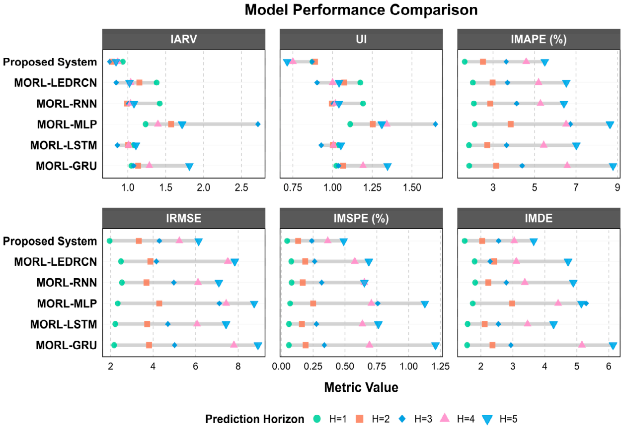
Note: Bold values indicate the results of the proposed system for ease of comparison.

and Figure 5 present the evaluation metrics for the different base predictors.

(1) At $H=1$, all models benefit from processing the inputs through M-MIDAS, although the performance differs across architectures. Among the individual models, RNN achieved relatively strong results, with the lowest IARV of 0.9099 and IMAPE of 1.6585. However, the proposed system further improved performance by reducing the IMAPE to 1.6328 and IRMSE to 1.9544, outperforming all individual models. In addition, the UI (0.8733) was lower than those of GRU and LSTM, indicating a more stable interval estimation. These results suggest that the proposed system provides consistent gains, even when the base models perform well.

(2) At $H=2$ and $H=3$, the performance differences between the models become more evident. The proposed system achieved the lowest IARV values of 0.7912 and 0.7605, respectively, and consistently outperformed all individual models in IMAPE, IMSPE, and IRMSE. In contrast, although recurrent models such as LSTM and RNN remain competitive in certain metrics, their performance became less stable across the evaluation criteria. This indicates that increasing the horizon length amplifies the advantage of the integrated modeling system over standalone architectures.

(3) At longer horizons, the performance gap persisted, with individual models showing increased instability across metrics. In contrast, the proposed system maintained a lower IMAPE and IRMSE while reducing IMSPE and UI, indicating better control over both error magnitude and interval variability. The additional reduction in the IMDE further confirms its ability to capture structured prediction dynamics under more challenging forecasting conditions.

Overall, these results indicate that although M-MIDAS improves the predictive capability of all base models, individual architectures alone are insufficient to maintain stable performance across increasing forecasting horizons. By integrating complementary modeling strengths, the proposed system achieves more accurate and robust interval-valued predictions.

4.4. Performance of the Proposed LE-DRCN

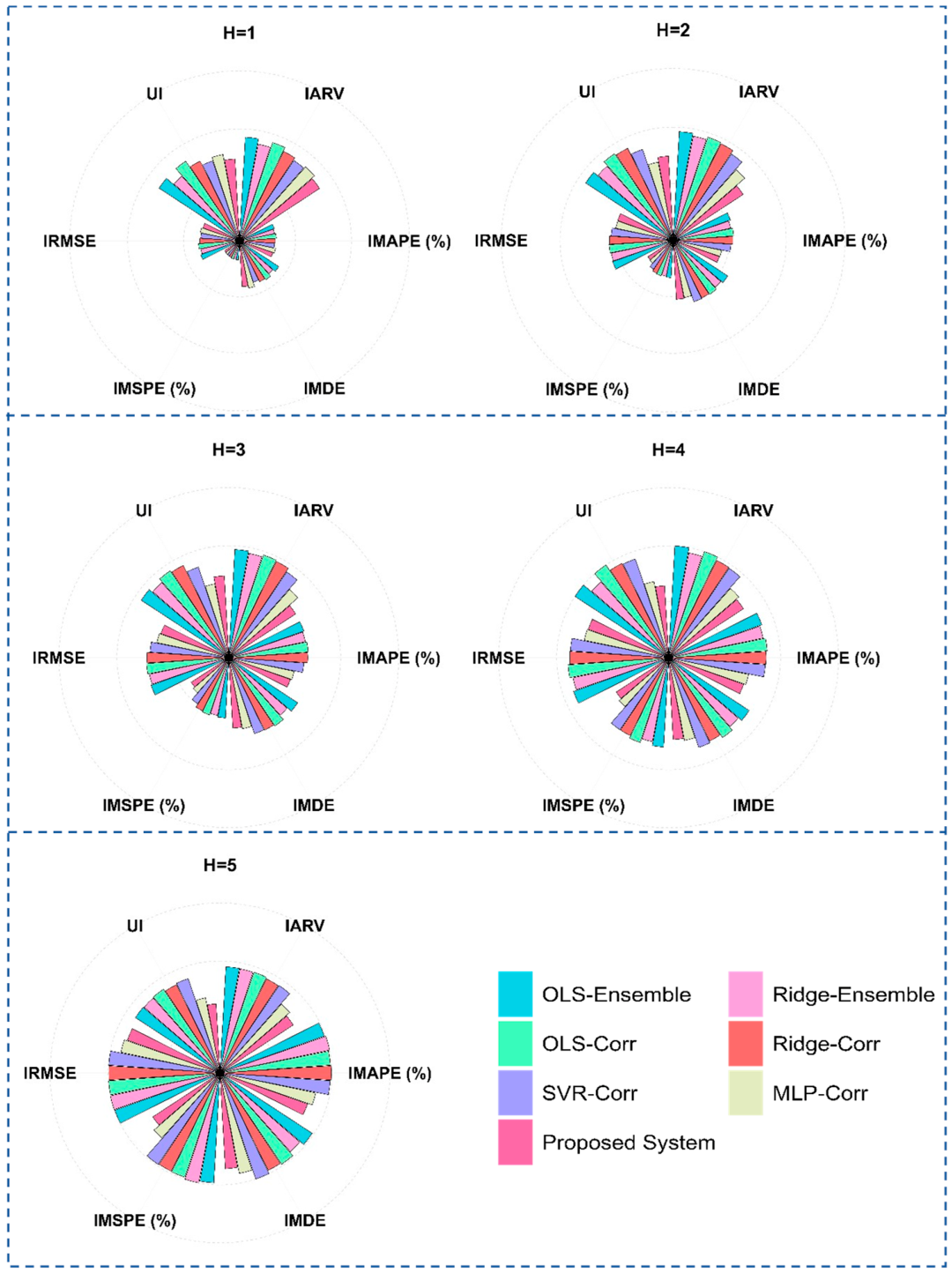
To answer RQ4, this subsection examines whether different ensemble strategies can effectively improve forecasting accuracy and stability. Specifically, we compared simple linear aggregation methods, including ordinary least squares (OLS)-Ensemble and Ridge-Ensemble, with a series of error-correction-based ensemble strategies, namely, OLS-Corr, Ridge-Corr, support vector regression (SVR)-Corr, and MLP-Corr, to evaluate the effectiveness of different fusion mechanisms in multistep forecasting settings.

Table 8. Comparison of different ensemble strategies.

Step	Model	IARV	UI	IMAPE (%)	IRMSE	IMSPE (%)	IMDE
H = 1	OLS-Ensemble	1.0237	1.0480	1.7285	2.1169	0.0560	1.5403
	Ridge-Ensemble	0.9646	0.9305	1.6491	2.0052	0.0512	1.4119
	OLS-Corr	1.0237	1.0480	1.7285	2.1169	0.0560	1.5403
	Ridge-Corr	0.9791	0.9587	1.6554	2.0233	0.0516	1.4757
	SVR-Corr	0.9499	0.9023	1.6100	1.9614	0.0490	1.3917
	MLP-Corr	0.9726	0.9460	1.7234	2.0432	0.0503	1.5868
	Proposed System	0.9345	0.8733	1.6328	1.9544	0.0463	1.4947
H = 2	OLS-Ensemble	1.0660	1.1364	3.2854	3.6936	0.1841	2.3015
	Ridge-Ensemble	1.0356	1.0725	3.1542	3.6326	0.1775	2.2053
	OLS-Corr	1.0660	1.1364	3.2854	3.6936	0.1841	2.3015
	Ridge-Corr	1.0547	1.1123	3.2314	3.6587	0.1799	2.2651
	SVR-Corr	1.0150	1.0302	3.0993	3.5552	0.1673	2.2852
	MLP-Corr	0.9115	0.8309	2.5448	3.3017	0.1378	2.0080
	Proposed System	0.7912	0.8895	2.5113	3.3270	0.1325	2.0404
H = 3	OLS-Ensemble	1.0738	1.1530	4.5963	5.0355	0.3492	3.0620
	Ridge-Ensemble	1.0497	1.1018	4.5017	4.9363	0.3379	2.8360
	OLS-Corr	1.0738	1.1530	4.5963	5.0355	0.3492	3.0620
	Ridge-Corr	1.0628	1.1295	4.5525	4.9839	0.3418	2.9966
	SVR-Corr	1.0193	1.0389	4.3014	4.7889	0.3157	2.9714
	MLP-Corr	0.8871	0.7870	3.7295	4.3954	0.2556	2.6316
	Proposed System	0.7605	0.8720	3.6356	4.2930	0.2396	2.5553
H = 4	OLS-Ensemble	1.1143	1.2418	5.8916	6.3277	0.5544	3.6627
	Ridge-Ensemble	1.0564	1.1159	5.7359	6.1060	0.5260	3.4812
	OLS-Corr	1.1143	1.2418	5.8916	6.3277	0.5544	3.6627
	Ridge-Corr	1.0765	1.1589	5.8114	6.1809	0.5363	3.5128
	SVR-Corr	1.0705	1.1459	5.7701	6.1599	0.5373	3.5885
	MLP-Corr	0.9041	0.8174	4.7349	5.2846	0.3844	3.1378
	Proposed System	0.8662	0.7503	4.5982	5.2332	0.3650	3.0439
H = 5	OLS-Ensemble	1.0521	1.1070	6.6906	7.0861	0.7019	4.2622
	Ridge-Ensemble	1.0486	1.0996	6.7736	7.1098	0.7152	4.0606
	OLS-Corr	1.0521	1.1070	6.6906	7.0861	0.7019	4.2622
	Ridge-Corr	1.0369	1.0752	6.7344	7.0518	0.6995	4.1995
	SVR-Corr	1.0437	1.0893	6.6771	7.0774	0.7047	4.3388
	MLP-Corr	0.8968	0.8043	5.8132	6.3495	0.5401	3.9218
	Proposed System	0.8451	0.7142	5.4931	6.1394	0.4900	3.6523

Note: Bold values indicate the results of the proposed method for ease of comparison.

and Figure 6 present the comparative results across multiple forecasting horizons.

(1) At the H = 1 forecasting horizon, the performance differences among the models were relatively moderate. Linear ensemble methods, such as OLS-Ensemble and Ridge-Ensemble, do not consistently outperform the simple averaging strategy, suggesting that static linear weighting is insufficient to fully exploit the complementary information from the baseline models. In contrast, nonlinear correction strategies demonstrate stronger adaptability. For instance, SVR-Corr achieved a competitive IARV of 0.9499 and an IRMSE of 1.9614. The proposed model further reduced the IARV to 0.9345 and obtained the lowest UI value of 0.8733, indicating its superior interval-valued compactness and stability.

(2) When the forecasting horizon was extended to H = 2 and H = 3, the advantages of the advanced ensemble strategies became more pronounced. The performance of traditional ensemble methods deteriorated in some cases, underperforming the leading expert models. This highlights their limited ability to handle error accumulation. In contrast, the correction-based methods effectively mitigate this issue. For example, MLP-Corr reduced the IMAPE to 2.5448 at H = 2 and 3.7295 at H = 3. The proposed model consistently delivered the best overall performance, achieving the lowest IARV values of 0.7912 and 0.7605 and the lowest IMSPE values of 0.1325 and 0.2396 at H = 2 and H = 3, respectively. These results demonstrate the effectiveness of the method in capturing nonlinear dependencies and correcting systematic errors.

(3) When the horizon was further extended to H = 4 and H = 5, the better performance of the proposed model became more evident. While most benchmark methods suffer from significant performance degradation due to accumulated uncertainty, our model maintains robust improvements across all evaluation metrics. At H = 4, it achieved the lowest UI value of 0.7503 and reduced the IMAPE to 4.5982, clearly outperforming MLP-Corr. At H = 5, the model achieved the best performance across all key metrics, including an IARV of 0.8451, IMAPE of 5.4931, IRMSE of 6.1394, and IMSPE of 0.4900, demonstrating its strong robustness in multistep forecasting.

In summary, the empirical results consistently demonstrate that ensemble methods based on residual correction systematically outperform those that directly combine forecasts. In contrast to other correction-based approaches, the proposed model achieves a good balance between flexibility and robustness, delivering comprehensively stable performance in multistep interval-valued forecasting scenarios.

4.5. Component Contribution Analysis

To partially address RQ5 and evaluate the contribution of the major modules in the proposed system, we performed a component-wise ablation analysis by removing or replacing key components and comparing the resulting variants with the full model. The system consists of three main modules: the MORL-based feature-selection mechanism, M-MIDAS for multisource frequency alignment, and LE-DRCN for dynamic ensemble learning. To isolate the role of multisource alignment, M-MIDAS was replaced with the conventional single-input MIDAS, which does not support the parallel integration of heterogeneous sources. For the ensemble stage, LE-DRCN was substituted with conventional static aggregation schemes, allowing a direct comparison between adaptive and nonadaptive ensemble strategies.

The results in

Table 9. Contribution of key components in the proposed system.

Step	Model Variant	M-MIDAS	LE-DRCN	The Decrease in Performance (%)
				IARV	UI	IMAPE	IRMSE	IMSPE	IMDE
H = 1	Full Model	✔	✔	—	—	—	—	—	—
	w/o LE-DRCN	✔	✘	3.62	6.28	7.33	2.10	17.03	3.90
	w/o M-MIDAS	✘	✔	32.29	25.66	19.47	21.44	41.32	17.16
	Traditional MIDAS	△	✔	17.34	17.87	10.33	11.85	24.47	10.64
	Best single model	✔	✘	10.14	19.24	5.59	8.39	19.34	11.08
H = 2	Full Model	✔	✔	—	—	—	—	—	—
	w/o LE-DRCN	✔	✘	17.71	3.79	11.12	1.07	12.66	8.78
	w/o M-MIDAS	✘	✔	31.35	17.14	15.71	14.04	29.56	15.46
	Traditional MIDAS	△	✔	27.47	14.84	16.55	9.43	26.76	8.09
	Best single model	✔	✘	20.99	11.31	17.33	5.45	18.86	12.90
H = 3	Full Model	✔	✔	—	—	—	—	—	—
	w/o LE-DRCN	✔	✘	19.49	2.26	8.72	5.39	15.31	11.51
	w/o M-MIDAS	✘	✔	10.27	3.38	1.62	3.60	8.62	8.45
	Traditional MIDAS	△	✔	30.41	16.59	13.78	13.00	23.67	18.16
	Best single model	✔	✘	24.06	13.04	14.11	9.70	22.16	16.18
H = 4	Full Model	✔	✔	—	—	—	—	—	—
	w/o LE-DRCN	✔	✘	8.18	15.71	10.49	6.77	17.01	10.13
	w/o M-MIDAS	✘	✔	16.39	26.28	12.98	14.36	44.08	9.81
	Traditional MIDAS	△	✔	1.03	16.90	4.36	2.81	7.24	3.77
	Best single model	✔	✘	12.62	23.65	14.44	10.39	23.69	12.70
H = 5	Full Model	✔	✔	—	—	—	—	—	—
	w/o LE-DRCN	✔	✘	10.29	21.63	12.81	6.12	20.14	3.69
	w/o M-MIDAS	✘	✔	21.00	45.79	18.89	27.71	40.24	29.42
	Traditional MIDAS	△	✔	20.49	41.29	18.1	16.42	42.82	13.96
	Best single model	✔	✘	18.51	40.45	19.68	12.82	37.92	10.70

Note: “✔” indicates the full model with the corresponding module included, “✘” indicates the model variant with the corresponding module removed, “—” indicates the baseline full-model configuration used for comparison, and “△” denotes a variant where the proposed M-MIDAS module is replaced by a standard single-source MIDAS model without multi-source frequency alignment.

quantify the contribution of each module. The decrease in performance (%) of each ablated variant compared with that of the full model is reported. In particular, removing M-MIDAS caused substantial degradation at H = 1 and H = 2, with IARV increasing by 32.29% and 31.35%, and IMSPE increasing by 41.32% and 29.56%, respectively. This indicates that multisource frequency alignment plays a critical role in preserving interval information and improving predictive accuracy. Moreover, replacing LE-DRCN with static ensemble strategies also led to consistent performance losses, especially at H = 3 and H = 4, where IARV deteriorated by 19.49%, and UI and IMSPE increased by 15.71% and 17.01%, respectively. Overall, these results suggest that the effectiveness of the proposed system relies on the complementarity between the structured multisource representation and adaptive ensemble learning.

4.6. Interpretability Analysis

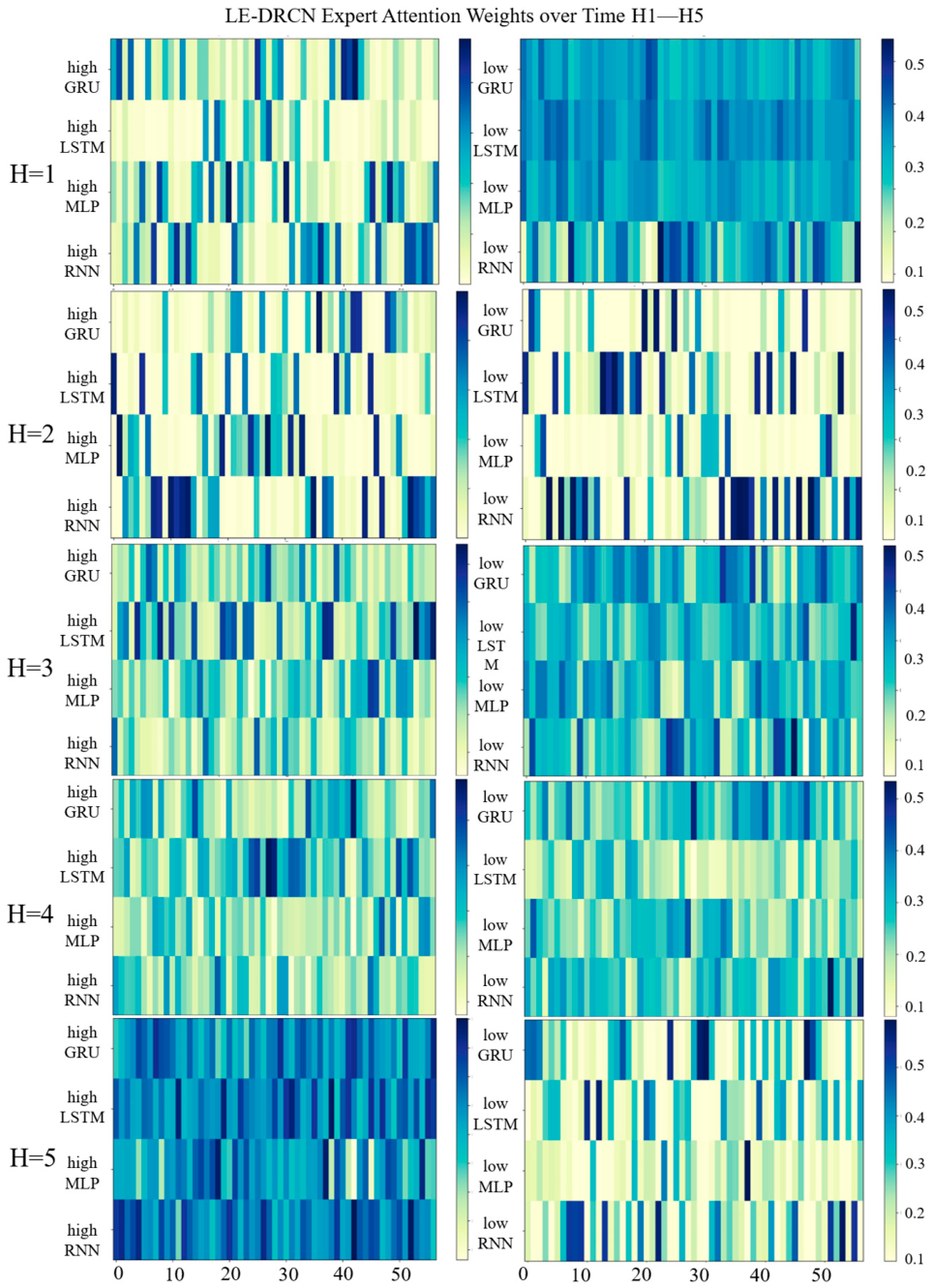
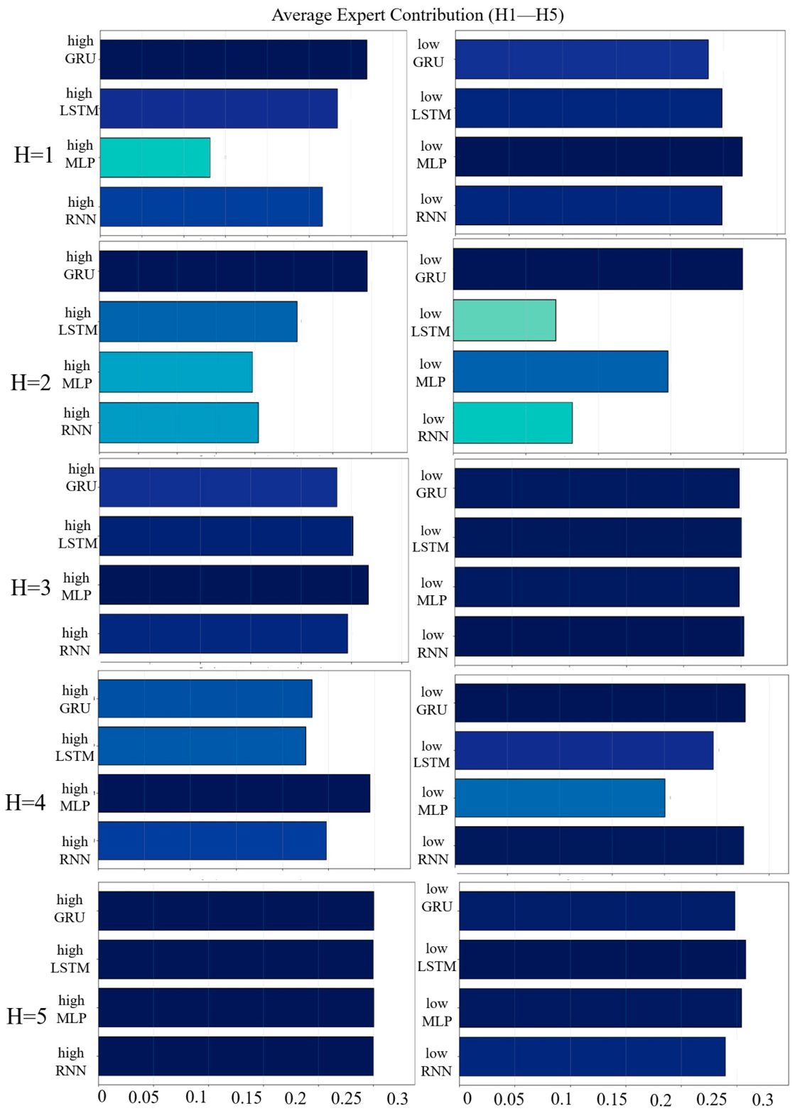
To answer RQ5 and clarify the internal coordination mechanism of the LE-DRCN ensemble model, we examined how the model dynamically adjusted its reliance on different expert neural networks across forecasting tasks through temporal attention patterns and average expert contributions.

Figure 7 presents the temporal evolution of the attention weights, showing how the model allocates importance to different expert models over time. Different colors represent the magnitude of attention weights, where darker blue indicates higher attention values and lighter colors indicate lower attention values. This evolution reveals a systematic temporal structure in attention allocation rather than random fluctuations. For one-step-ahead forecasting, attention tends to concentrate on specific expert models at particular time points, particularly on recurrent architectures, such as GRU and LSTM. As the forecasting horizon extends to multiple steps ahead, the attention patterns become more dispersed across different expert types, suggesting that multistep prediction tasks require a broader integration of diverse modeling approaches. The results for the highest-price forecasting scenario exhibited more variable attention patterns than those for lowest-price forecasting, with attention shifting more frequently among experts.

Figure 8 shows the average contribution of each expert model across all forecasting horizons, where different colors represent different expert models, with darker blue indicating higher contribution values and lighter colors indicating lower contribution levels. The results confirm that LE-DRCN adaptively weighs different neural network architectures according to task characteristics. At the single-step horizon, recurrent models, including GRU and LSTM, dominated the contributions, reflecting their architectural advantages in capturing short-term temporal patterns. As the forecasting horizon increased, expert contributions became more balanced across different model types, with the MLP and RNN architectures playing increasingly important roles. The variation in expert contributions is more pronounced for highest-price forecasting, particularly at intermediate horizons, where certain experts show sharply reduced contributions, while others maintain stable weights, indicating greater ensemble flexibility when forecasting upward price movements.

These patterns demonstrate that the LE-DRCN module automatically adapts its ensemble strategy to different prediction contexts. The concentration of attention and expert weights on recurrent models at short horizons reflects the importance of capturing recent temporal dynamics, whereas more dispersed patterns at longer horizons indicate the need to integrate complementary modeling approaches as prediction uncertainty increases.

5. Conclusions

5.1. Key Findings and Implications

This study developed a unified multi-step forecasting system for carbon price prediction by integrating the MORL-based feature selection mechanism, M-MIDAS module, and LE-DRCN residual correction. The empirical results show that the proposed system consistently outperforms benchmark models across one- to five-step-ahead horizons, indicating that jointly modeling feature relevance, mixed-frequency dependencies, and residual structures improves predictive performance.

From a methodological perspective, three main findings emerged. First, the strong performance of the MORL-based mechanism, which consists of feature selection with frequency decomposition, indicates that market factors affect carbon prices through distinct temporal channels, with some variables contributing persistently across scales and others dominating specific horizons, highlighting the importance of multiscale interactions. Second, the ablation results confirmed that the M-MIDAS module effectively integrates mixed-frequency information into a unified representation. Third, the LE-DRCN module was found to exhibit horizon-dependent behavior in which recurrent structures contribute more to short-term forecasts, whereas diversified expert combinations enhance performance at longer horizons.

These findings have several implications for the application of forecasting models in carbon markets. The frequency-decomposed feature importance provides interpretable signals of the dominant drivers of carbon price movements across different temporal scales. When specific macro-financial or energy-related variables exhibit persistently high importance, this indicates an increased sensitivity of carbon prices to external market conditions; under such situations, monitoring efforts should be concentrated on these identified channels to better track potential spillover effects. Meanwhile, the attention distribution patterns obtained from the LE-DRCN module further provide regime-dependent informational signals. Concentrated attention on a small number of experts is associated with relatively stable market conditions, under which model outputs can be interpreted with higher confidence for directional assessment. In contrast, dispersed attention across multiple experts reflects heightened uncertainty and heterogeneous information processing, suggesting that decision-making should shift toward more conservative or risk-aware strategies with reduced reliance on single-point forecasts. In addition, error patterns across forecasting horizons may provide useful supplementary signals for market monitoring. Periods of unusually large prediction errors may indicate that the market is undergoing abnormal fluctuations or is facing information conditions that are not fully captured by the model. Therefore, such deviations may serve as a practical cue for closer monitoring and a more cautious interpretation of the forecasting results.

5.2. Limitations and Future Work

Despite these contributions, this study has several limitations that warrant further investigation. First, although the rolling-window training scheme and dynamic expert selection improve the model adaptability, the current system does not explicitly account for policy-driven structural changes. Future research could therefore incorporate policy-sensitive variables, regime-switching structures, or online updating mechanisms to better model the structural breaks induced by institutional adjustments.

Second, this study focused on China’s national carbon market to maintain institutional consistency. However, the system proposed in this study does not consider interactions between national and regional pilot carbon markets. A future research extension would be to develop a joint forecasting model that explicitly captures the interaction between regional and national carbon markets. Finally, future research may extend the current system by incorporating probabilistic forecasting methods, richer policy and market microstructure information, and more realistic applications, such as hedging and carbon-related portfolio management.