


Abstract
Decision theories based on cognitive consistency understand decision-making as the process of constructing a coherent representation of reality, capable of providing a reliable causal map that connects actions to consequences. Rejecting assumptions concerning preferences and utility functions, they single out the quest for a coherent representation of reality as the one single factor driving human behaviour. Decision theories based on constructing coherence are justified by free-energy minimisation and supported by computational network models, but they lack a proper mathematical framework. In this article I combine Evidence Theory with Quantum Logic to offer a scaffolding structure to construct coherent representations. I illustrate this framework with stylised examples drawn from medical diagnoses and the BioTech industry.
1. Introduction
Subjective Expected Utility Maximisation (SEUM) is by far the most common decision theory, indeed the only decision theory that is being employed in economics and from there diffused into other disciplines. As many readers may know, SEUM assumes that individuals have preferences and that they express these preferences by associating numerical utility values to the consequences of their choices, which in their turn occur with subjectively evaluated probabilities. Consequently, the one alternative is selected, whose consequences have the highest expected utility value.
The cognitive processes that originated those preferences and those subjective probability evaluations lie outside the scope of SEUM. Rather, the theory assumes that preferences are given and that probabilities are evaluated, somehow; once these data are available, the one best choice is computed. I contend that these limitations confine SEUM to decision problems that are sufficiently stable for preferences to have been attained and probabilities to have been assessed. Indeed, SEUM is appropriate for settings where some sort of equilibrium has been reached, which is what economics most often assumes.
From its very foundation, SEUM is an individual theory of decision-making. Thus, it understands collective decisions as deriving from matching individual preferences as epitomised by Game Theory. Unsurprisingly, applications of Game Theory based on SEUM are also concerned with equilibrium states.
Empirically, quite often, SEUM fails to describe actual human behaviour [1,2,3,4]. However, since SEUM descends from a set of reasonable postulates, it claims to have a prescriptive value as a theory of rational decision-making [5]. Moreover, most observed deviations of actual behaviour from SEUM prescriptions can be explained away by means of non-linear transformations (e.g., Prospect Theory) [6,7], sub-additive probabilities [6,8], or incomplete preferences [9,10,11].
Nonetheless, there exists one piece of empirical evidence that cannot be reconciled with SEUM. The seemingly unproblematic assumption that humans carry out separate evaluations of probability and utility, which is essential for SEUM, has been repeatedly disconfirmed [12,13,14,15,16,17,18]. And this disturbing result has been replicated by a number of independent researchers along several decades [19,20,21,22,23,24,25,26,27]. This finding does not affect the normative status of SEUM—one can still maintain that rational decision-makers should evaluate utilities and probabilities independently of one another, even if they often do not—but, unlike other empirical deviations, it cannot be reconciled with SEUM by means of slight modifications to the basic model.
According to the above experiments, humans rather focus on one salient aspect of a decision problem, ignoring or distorting others in order to be able to make a decision. This suggests that brains maximise the coherence between their experiences and their mental representations, constructing causal explanations that provide orientation in an otherwise uncertain environment. Thus, individuals may express “preferences” and evaluate “probabilities” insofar as their environment is relatively stable and their mental representations are sufficiently successful, but those are not the prime movers of decision-making.
Moreover, since individual decisions are made through interactions with an environment that includes other human beings, there is no such thing as individual decisions independently of collective decisions. Collective decisions are rather seen as the global outcome of individual adjustments to a social environment that they themselves construct [28,29,30,31,32,33,34,35,36,37].
Several mathematical or computational tools support decision theories based on cognitive consistency (Henceforth, the expressions “cognitive consistency” and “constructing coherence” will be used as synonyms). On the one hand, physical considerations on free-energy minimisation (FEM) offer necessary conditions why brains should maximise coherence between decisions and environmental feedback [38,39,40,41,42,43,44,45,46,47] (see Appendix B). In particular, FEM can explain several findings in neurophysiology, from the existence of mirror neurons [48] to phase synchronisation of electrical signals [44]. Furthermore, it offers a rationale for collective behaviour in epistemic communities [49], for the construction of social scripts [50], the development of a theory of mind [51] as well as the emergence of hierarchical structures among living beings [52,53,54].
On the other hand, Constraint Satisfaction Networks (CSNs) [55,56,57,58,59,60] offer a computational model of coherence-seeking decision-making. CSNs are neural networks whose nodes represent possibilities, or concepts, or propositions linked to one another by either excitatory or inhibitory connections (an excitatory connection from A to B means “A implies B” whereas an inhibitory connection means “A implies ¬ B”). CSNs are bi-stable systems that after a few oscillations eventually settle down into an equilibrium that expresses a coherent arrangement of available concepts (see Appendix A).
Notable applications of CSNs concern the elaboration of scientific theories by arranging empirical findings in a network of consistent causal relations, the evaluation of guilt or innocence in a trial by fitting testimonies in a coherent frame, as well as the arrangement of symptoms into diagnoses [55,61,62,63,64]. Recent extensions focus on collective decision-making by means of networks of networks representing individuals in groups and societies [65,66,67,68].
While FEM is a general principle that explains broad trends and CSNs are a computational model that handles specific problems, decision theories based on cognitive consistency lack a mathematical formalism comparable to SEUM. With this article, I want to take a step towards filling this gap.
Evidence Theory (ET) [69], also known as “Dempster–Shafer Theory” or “Belief Functions Theory,” is a mathematical theory of uncertain reasoning that takes as prototypical situation a judge evaluating testimonies or a detective examining cues [70,71]. This is quite different from Probability Theory (PT), whose prototypical situations are based on games of chance. I submit that since judges and detectives must evaluate the coherence of testimonies and cues, ET is an appropriate framework for theories of decision making based on the quest for coherence.
Specifically, I present an interpretation of ET where the useful and the likely are not disentangled from one another. This interpretation is uncommon, albeit coherent with the original aims of ET [72,73]. In particular, I make use of Smets’ Transferable Belief Model (TBM) of evidence combination [74,75] and extend the theory by means of Quantum Logic (QL) [76,77].
The rest of this article is organised as follows. The ensuing Section 2 introduces ET for closed and open worlds in Section 2.1 and Section 2.2, respectively. Subsequently, Section 3 and Section 4 offer logical bounds to novel concepts and propose heuristics to make sense of reactions in front of disconfirming evidence, respectively. Finally, Section 5 outlines the impact of assuming metric spaces, while Section 6 concludes.
2. An Unconventional Presentation of Evidence Theory
Following Smets [75], let us start by assuming that a sequence of empirical evidence arrives, upon which suitable magnitudes can be defined. Within this framework, the two cases of a closed and an open world are expounded in Section 2.1 and Section 2.2, respectively.
In PT, possibilities are mutually exclusive. This is a straightforward consequence of having chosen games of chance as the paradigmatic setting of uncertain reasoning—dice have distinct faces, roulettes have distinct slots, and so on. Consequently, possibilities are singletons. Let us denote any two of these isolated possibilities as , . Since they are singletons, they can be either distinct () or coincide () but they cannot intersect.
By contrast, judges may find that two testimonies reinforce one another in substantial respects, while at the same time differing from one another in certain details. Thus, ET understands possibilities as sets, which implies that two possibilities and can exist, for which .
Obviously, PT can reach this understanding by aggregating elementary possibilities, e.g., the possibility that an odd face of the die comes up is the union of either face 1, or 3, or 5 coming up. Indeed, one alternative—and more common—path to expound ET starts with a “basic probability assignment” and proceeds to define ET constructs within a PT-like framework.
Let us denote by the mass of evidence supporting possibility . Henceforth, it is generally assumed that albeit Section 5 discusses the possibility that in order to represent wavelike evidence [78,79,80].
Mass is exogenous information, similar in spirit to frequentist interpretations of probability. Later on, ET provides opportunities for personal generation of hypotheses, which brings it closer to subjective interpretations of probability.
Let us assume that incoming information takes the shape of bodies of evidence:
In ET, the possibility set is called frame of discernment (FoD), generally denoted by . The name itself conveys the idea that cognition is essential for a set of possibilities to be envisaged. Technically, this insight translates into not necessarily assuming that is a -algebra (A -algebra is closed under complement, countable union and countable intersection).
By contrast, this assumption is essential for PT because if the possibility set is a -algebra, all unions, intersections and complementations of all possibilities are automatically computed. In particular, complementation can generate a residual event (“anything else that may happen”) which makes the list of events exhaustive even if originally it was not.
If we have reasons to assume that the list of events that we are envisaging is exhaustive, then we can safely assume that the FoD is a -algebra. Under this assumption, it is correct to view ET as an extension of PT with possibilities defined as sets rather than singletons [81,82]. By contrast, if we have reasons to suspect that other possibilities may become available, then it is sensible not to assume that is a -algebra.
Here is one way to conceptualise this difference. Assuming that is a -algebra corresponds to assuming that human intelligence is algorithmic, as early Artificial Intelligence used to do in the 1950s [83,84]. By contrast, if is not a -algebra other views are possible, such as understanding intelligence as based on analogies enabled by distributed memories [85].
Indeed, assuming that the FoD is an algebra implies an obligation for the FoD to carry out logical operations. However, we shall see henceforth that FoDs that are not assumed to be algebras do not impair decision-makers to apply logical operators in a subset if they wish to do so [86]. ET does allow decision-makers to employ any logic they wish, but rejects the assumption that the system must automatically do it.
Henceforth, I assume that is not a metric space. This means that is given by their common elements, rather than the extent of their overlap. Possible extensions to a metric space are outlined in Section 5.
One important aspect where ET departs from standard PT (though maintaining similarities to sub-additive PT, see [87]) is in providing a means to acknowledge that the information carried by the bodies of evidence may be less than perfect. For instance, witnesses may have observed a murder while they were half-drunk, or a die may be suspected to be unfair. Whenever there is some reason to assume that some information is missing, a positive mass is assigned to the FoD. This is not distributed to the possibilities that are currently envisaged in .
If witnesses themselves are aware that their information may be unreliable, they themselves present evidence coming with a , , and so on. Or, if we suspect that a source is less than perfectly reliable, we may add a , to the original evidence. From this point onwards, the case of a closed world differs from that of an open world. These two cases are illustrated in Section 2.1 and Section 2.2, respectively.
2.1. A Closed World
In a closed world, ET may assume that the FoD is a -algebra, or not. In the first case, all unions, intersections and complementations are computed. In the second case, the FoD entails only those possibilities that the available empirical evidence suggests.
Let us assume that incoming bodies of evidence take the following shape:
Though not strictly necessary, bodies of evidence are generally normalised as follows:
Note that, since it can be , in general . This is quite different from PT, where the total mass of evidence is distributed among non-intersecting probabilities.
The judge or detective is assumed to combine the available bodies of evidence by means of Dempster–Shafer’s rule [69,88]:
where , , and where the s are defined by all possible intersections of the s with the s.
The s computed by Equation (2) are the components of a new body of evidence C that unites A and B. Note that Equation (2) also computes the new , but this computation requires that and . In practice, a judge may discount a less-than-perfectly reliable testimony X by adding a to it and normalising X by means of Equation (1).
The numerator of Equation (2) measures the extent to which the two bodies of evidence coherently support , whereas the denominator measures the extent to which they are not contradictory with one another. Specifically, the denominator of Equation (2) eliminates contradictory evidence by redistributing it among coherent evidence.
The outcome of Dempster–Shafer’s combination rule (2) is independent of the order in which evidence bodies are combined. If the bodies of evidence that are fed into Equation (2) have been normalised according to Equation (1), the outcome is normalised as well.
Once all available evidence has been combined into one single body of evidence Z, the judge or detective can use it to evaluate to what extent this evidence supports specific hypotheses. Note that while exogenous evidence may remind of frequentist interpretations of probability, hypotheses formulation is purely subjective.
Specifically, let us suppose that the judge or detective wants to evaluate to what extent a body of evidence supports hypothesis . The belief function expresses strict support for :
where by definition and .
By contrast, the plausibility function expresses partial support for :
where by definition and .
In general, . This derives from the fact that is supported only by the evidence that strictly supports , whereas also includes evidence that partly supports competing hypotheses.
Note that Equations (2)–(4) employ logical operators that the judge or detective defines in a subset [86]. Hypotheses can be generated by means of logical operators, though no assumption must be necessarily made in this respect.
Example: Zadeh’s Paradox
Lofti Zadeh criticised Dempster–Shafer’s combination rule (2) with the following paradox [89]:
Suppose that a patient, P, is examined by two doctors, A and B. A’s diagnosis is that P has either meningitis, with probability 0.99, or brain tumour, with probability 0.01. B agrees with A that the probability of brain tumour is 0.01, but believes that it is the probability of concussion rather than meningitis that is 0.99.
In this example, meningitis, tumour and concussion are meant as possibilities that mutually exclude one another, just like the faces of a die. Let us represent them as singletons , , . Let the two doctors provide two bodies of evidence A and B, respectively, that express evidence in probabilistic terms:
Since is the only non-void intersection between A and B, the body of evidence resulting from applying Equation (2) is and its numerical value is:
By applying Equation (3) one obtains . This conclusion is paradoxical because precisely was the diagnosis that had received the least support.
Zadeh’s paradox halted the acceptance of ET, originating a quest for combination rules that would perform better than Equation (2). Few researchers remarked that Zadeh’s example generates equally paradoxical results if Bayes’ rule is applied [90,91].
To see this, let us apply PT to Zadeh’s example. Since it is , and consequently . The only non-zero conditional probabilities are:
which trivially satisfy Bayes’ rule with .
The reason why both Dempster–Shafer’s and Bayes’ rule fail on Zadeh’s paradox is that both are based on intersecting possibilities (although Bayes’ Theorem pertains to PT, it is applied to events that generally include different outcomes and therefore intersect). In Zadeh’s paradox, the two doctors provide opposite diagnoses that allow for just a minimal intersection, which is the only conclusion that both rules can draw.
In a closed world, Zadeh’s paradox can be resolved in two ways [90,92]. The first consists of the patient suspecting that either doctor is wrong. In ET, this would amount to assume that either , or , or possibly both. In PT, this would require the non-standard assumption of sub-additive probabilities (see [87]). Since and , some positive mass could still be assigned to meningitis or concussion.
The second solution requires doctors to change their assessment of the symptoms that correspond to meningitis, concussion and tumour. For instance, if certain symptoms are compatible with both meningitis and tumour (), or with both concussion and tumour (), or with both meningitis and concussion (), the combination of the two bodies of evidence likely yields positive magnitudes for all three diagnoses.
If both solutions are employed, the two bodies of evidence become:
and Equation (2) generates the following combined evidence:
where the are measured by counting symptoms.
By feeding the numbers entailed in Z into Equations (3) and (4), the patient can compute the belief and plausibility of each diagnosis. Note that while the patient (the judge) can add and to the original diagnoses without questioning the doctors’ (the witnesses’) analyses, expressing the intersections between M, C and T requires doctors to disclose what symptoms they have observed and how they relate to one another.
2.2. An Open World
In an open world, the judge or detective is aware that novel possibilities may materialise, which eventually generate unexpected denouements. In order to express this state of mind, the FoD must be assumed not to be a -algebra.
Denouements are triggered by novel and surprising possibilities that contradict established relations of causes and effects, generating a state of radical uncertainty (also known as “Keynesian,” “true” or “ontological” uncertainty [93,94,95,96,97,98]) that concerns the appearance of novel possibilities, rather than probability distributions over given possibilities. Thus, one can take the amount of conflicting evidence as an appropriate measure of radical uncertainty [99,100,101].
In particular, following Smets [74,102,103] let us assume that in open worlds, conflicting evidence translates into . The rationale for this assumption is that conflicting evidence moves some mass of belief towards possibilities that cannot yet be defined [87].
Let us assume that incoming bodies of evidence take the following shape:
In an open world, normalisation includes :
In open worlds, Smets’ combination rule applies, which is essentially the numerator of Equation (2):
where , , and the s are defined by all possible intersections of the s with the s.
In Equation (2), the denominator redistributes conflicting evidence among non-conflicting possibilities. By contrast in Equation (6), since conflicting evidence is ascribed to , that denominator does not exist.
Let us assume that a combined body of evidence results from repeatedly applying Equation (6). Belief and plausibility functions now take the following form [91]:
where the second and third lines are different from Equation (3) which assumed and , respectively.
where the second and third lines are different from Equation (4) which assumed and , respectively.
Similarly to the closed-world case, Equations (6)–(8) employ logical operators that the judge or detective defines in a subset [86]. Similarly to the closed-world case, hypotheses can be generated by means of logical operators but no assumption is made in this respect.
One key difference with the case of a closed world is that when exceeds some threshold (see [104] for an experimental assessment), decision-makers—like judges and detectives—look for additional information, pay attention to previously neglected details, discard prominent evidence as irrelevant and formulate novel hypotheses. In ET, these activities appear as tightening and loosening the FoD [87,90,91,105,106]. Albeit this is a creative process, its rationale can be pinned down:
Like any creative act, the act of constructing a frame of discernment does not lend itself to thorough analysis. But we can pick out two considerations that influence it: (1) we want our evidence to interact in an interesting way, and (2) we do not want it to exhibit too much internal conflict.
Two items of evidence can always be said to interact, but they interact in an interesting way only if they jointly support a proposition more interesting than the propositions supported by either alone. (…) Since it depends on what we are interested in, any judgement as to whether our frame is successful in making our evidence interact in an interesting way is a subjective one. But since interesting interactions can always be destroyed by loosening relevant assumptions and thus enlarging our frame, it is clear that our desire for interesting interaction will incline us towards abridging or tightening our frame.
Our desire to avoid excessive internal conflict in our evidence will have precisely the opposite effect: it will incline us towards enlarging or loosening our frame. For internal conflict is itself a form of interaction—the most extreme form of it. And it too tends to increase as the frame is tightened, decrease as it is loosened.(Glenn Shafer [69], Ch. XII)
In purely set-theoretical terms, tightening the FoD consists of refining a set. However, random refinement would not amount to tightening the FoD, just like Sherlock Holmes does not explore possibilities at random. Tightening takes place with respect to the causal relations that link possibilities to one another in the FoD, for instance because some of them do not square well with the others and solving problems is, at least to some extent, “interesting” for human brains.
In purely set-theoretical terms, loosening the FoD consists of coarsening a set. However, this coarsening does not take place at random but rather with the aim of simplifying causal relations by discarding details that the emerging understanding makes irrelevant.
Tightening and loosening the FoD is an essential activity for ET to operate in an open world. Only by tightening and loosening the FoD can decision-makers hope to make sense of the novelties that initially destroyed the received wisdom. More on this in Section 3 and Section 4.
Example: Recognising COVID-19
If the scene described by Zadeh’s paradox had happened in the real world, patients experiencing would have rushed to consult a third doctor [90,92]. But this cannot be told within the narrow framework of Zadeh’s paradox, because decision-makers facing conflicting evidence cling to the tiniest details offered by real experience in order to assemble a sensible explanation. The surprising recognition that COVID-19 had already reached Europe is a much richer example.
In 2019 and until the early 2020 it was generally assumed that, by analogy with previous epidemics, COVID-19 would take a long time to reach Europe from China. On 18 February 2020, a man aged 38 reached the emergency department of a small hospital in Codogno, Italy, exhibiting mild respiratory difficulties. He was diagnosed with a pneumonia and sent back home with self-medication instructions [107].
This was the FoD at , illustrated on the left portion of Figure 1. The initial body of evidence perceived in the emergency room might be represented as follows:
where stands for “mild respiratory difficulties”.
Figure 1.
Possibilities in the FoD at , and . At and again at the FoD was tightened because novel possibilities appeared. At the FoD was loosened because the initial possibility was deleted.
At the patient returned to the emergency department with heavy respiratory difficulties, which commanded immediate hospitalisation. A second body of evidence had arrived, incompatible with the first one:
where stands for “heavy respiratory difficulties”.
Since , the available evidence was contradictory. ET would not reach any definitive conclusion, except that so strong contradictory evidence suggested . Now, the world had been opened, and the FoD had to be tightened and loosened while looking for novel possibilities.
An anaesthesiologist interrogated the patient’s wife, who reported that her husband had met someone who had just come back from China [107]. Thus, at a new possibility entered the FoD, namely, that the patient had received the virus from someone who had been in an infected area:
where stands for “COVID”.
At and again at the FoD was tightened, because new possibilities were added. At that stage, the evidence was as depicted in the right portion of Figure 1. A “COVID-19” hypothesis could be formulated, and could be computed for and COVID-19.
At the analyses carried out by a National Laboratory (no quick tests were available in the early days) confirmed the COVID-19 diagnosis. The FoD could be loosened, discarding the initial evidence that supported a light pneumonia. From that point in time onwards, procedures returned to the assumption of a closed world.
Notably, subsequent investigations on the person whom the patient had met, the one who had returned from China, highlighted that she had not been infected by COVID-19. The origin of the infection of the first case detected in Europe was never discovered, though it was later ascertained that the virus had been circulating in other areas for several months [107].
This detail is remarkable, because it shows that once the world had been opened by contradictory information, decision-making became sensitive to cues of any sort, including false ones. Remarkably, even false cues were useful to direct FoD restructuring.
Obviously, this is generally not the case. Double-checking the consistency of evidence—in this case, the analyses carried out by the National Laboratory—is essential in order not to close the open world onto a fixed set of possibilities that might be just as limiting as the initial ones.
3. The Quantum Logic of Tightening and Loosening
Both Dempster–Shafer’s (2) and Smets’ (6) combination rules yield results that are independent of the order in which different bodies of evidence are considered. The judge or detective is assumed to contemplate the available evidence in a timeless space, limiting themselves to evaluate the support for alternative hypotheses whose origin is left unspecified. However, if , the FoD must be tightened and loosened and, in this process, novel hypotheses must be conceived.
In the FoD, possibilities overlap to the extent that they are coherent with one another, and possibilities are coherent insofar as they are embedded in causal relations. If causes , that appears as . If and are independent of one another but they both concur to , that appears as , , . In order to tighten and loosen the FoD, it is necessary to work at the level of the causal mappings that connect possibilities and identify hypotheses.
A cognitive map is a graph whose nodes represent concepts, linked by edges that represent causal relations. Cognitive maps can be assumed to provide orientation to decision-makers on what consequences might follow from specific decisions, independently of probabilistic evaluation. In social sciences, cognitive maps are eventually extracted from texts or interviews [108,109].
Occasionally, cognitive maps may entail loops insofar as decision-makers are able to envisage feedback that generates vicious or virtuous circles. However, the final outcome of these loops—as they are envisaged by decision-makers—can be generally lumped into a broader concept. After this transformation, cognitive maps can be represented as partially ordered sets where causality is the ordering relation.
In particular, let us represent a cognitive map as a Hasse diagram where each layer entails one body of evidence, whose possibilities are eventually ordered by causal relations with respect to those in the previous and subsequent layers. Let us understand the FoD as the projection of this diagram onto the possibility space where the causal links propagating from the upper starting nodes specify the inclusions and intersections of the possibilities entailed in the bodies of evidence below. Note that, contrary to basic ET, during the process of tightening and loosening the FoD the sequence of arrival of bodies of evidence matters for what causal relations are envisaged.
Figure 2 illustrates this representation with bodies of evidence , . Bodies of evidence are still combined by means of either Dempster–Shafer’s rule (2) or Smets’ rule (6), but which possibilities are being considered in each body of evidence depends on the causal relations that are being envisaged. Hypotheses appear at the bottom and in principle can include any possibility entailed in any body of evidence.
Figure 2.
A Hasse diagram representing an unspecified number of bodies of evidence whose elements are (partially) ordered by means of causal relations. In the traditional, static representation of ET, these causal relations are necessarily translated into set-theoretical relations and their ordering can be ignored because the FoD is not supposed to be tightened or loosened.
The following example illustrates why the sequence of exploration of possibilities and arrival of bodies of evidence matters for the final result. Consider a detective story. Typically, some detail that appears irrelevant to the police becomes a fundamental clue that suggests the amateur-detective to ask certain questions to certain people, obtaining key evidence. Even if this evidence is combined according to rules where the sequence is irrelevant, that specific clue directed the amateur-detective towards a path-specific investigation.
In an open world, triggers FoD tightening and loosening in search for a novel cognitive map. As the example of COVID-19 recognition suggests, tightening consists of conceiving novel possibilities out of hidden cues and serendipitous hints; loosening eventually follows, simply because possibilities that have become irrelevant can be lumped together or discarded.
This sort of abductive logic cannot be formalised and standardised to the extent that SEUM has optimised the process of selecting one out of a given set of opportunities. However, abduction is still a logical process. Specifically, the decision not to decide arises from the coexistence of contradictory evidence, much like quantum physics admits indeterminate states that eventually coalesce into the observation of either one or another magnitude [110,111]. Without claiming any quantum-physical foundation for the decision not to decide, elements of QL can be usefully employed to specify certain boundaries within which tightening must confine itself [76,77,112]. (In order to adapt QL to cognitive maps, I loosened structural requirements by substituting lattices with posets).
Let denote a piece of information entailed in a body of evidence. QL admits indeterminate states by assuming that any can have several complements. Conditions are the same as for the usual complementation, except that quantum complementation is not unique:
In PT, unicity of complementation ensures that -algebras are exhaustive possibility set. By contrast, ET rejects complementation altogether. With quite a smart move, QL accepts complementation but makes it innocuous by assuming that it is not unique. In practice, non-unicity of complements allows foreign possibilities to enter the FoD [76,77,112].
Quantum physics employs the orthomodularity condition because it is generally concerned with infinite-dimensional spaces. However, since cognitive maps are necessarily finite, the stricter modularity condition can be expected to hold:
if and .
Modularity allows Boolean logic to apply to specific areas of the cognitive map. This does not impair hypothesis formulation to be governed by QL.
With both (11) and (12) as , logical propositions are distributive with respect to ∧ and ∨. By contrast, lacking the distributive property, certain propositions are undecidable in QL. This corresponds in quantum mechanics to indefinite states and, in decision-making, to deciding not to decide.
Non-distributivity also has the consequence that any two logical propositions are not commutative with respect to ∧ and ∨ [113]:
Inequalities (13) and (14) apply to several experiments on decision-making that contradict Boolean logic, such as the order effect and the conjunction fallacy [76,114,115,116]. However, the observation that QL describes experiments where Boolean logic fails is not an explanation of why QL works.
QL may be thought of as singling out the sets of coherent concepts among which CSNs make a choice by readjusting their relative weights (see Appendix A). What one observes in CSNs is that one concept works as the tipping point that drags all others towards a coherent arrangement of causal relations [55,62,117].
This is quite important an insight. However, a mathematical framework that works at a higher level of generality should be able to express how those two (or more) sets of coherent concepts arise.
Example: BioTech in 1990
Throughout the 1980s, the still infant BioTech industry understood itself as the cradle of a new generation of pharmaceutical companies. Biotech companies were producing patents that they sold to large pharmaceutical companies—the so-called “Big Pharmas”—and those companies were their model. However naive such expectations may appear in retrospect, Biotechs vastly underestimated the technical and financial difficulties of producing and marketing medical drugs.
The analysis of the annual reports of a specialised consultant highlights that the cognitive maps of BioTech companies changed very little from the early 1980s through 1989 [118]. Suddenly, in 1990 BioTech companies realised that the Big Pharmas were not quietly waiting to be displaced. Instead, they were carefully designing the contracts that they stipulated with BioTech startups in ways that would enable them to control the knowledge base on which each single drug had been developed, impairing small BioTech companiess to reuse it to develop other drugs. Those contracts were, in business jargon, “Poison Pills.” The Big Pharmas expected to become able to develop recombinant-DNA technology in-house, ultimately driving the small BioTech companies out of the market. The 1990 cognitive map of BioTech companies extracted from consultant’s reports reflects their despair in realising this [118]. This map is much smaller than the previous ones, many new concepts had superseded those of the previous years, with “Poison Pills” now taking the central stage.
However, in subsequent years, the Big Pharmas learned that recombinant-DNA technology required a degree of exploration that their carefully designed research plans found difficult to accommodate. At the same time, BioTech companies realised that producing and marketing drugs was quite different a business from selling patents. A new series of cognitive maps ensued from 1991 onwards, quite similar to the pre-1990 ones except that “contracts with clear exit clauses” now appeared as a key concept [118].
Figure 3 illustrates the essential elements of BioTech companies’ cognitive maps until 1989 (left), in 1990 (centre) and since 1991 (right), simplified and arranged as Hasse diagrams. The 1990 map entails novel concepts (in red) that upset the previous causal relations. From 1991 onwards cognitive maps are similar to the pre-1990 ones, except that they entail a key concept (in green) concerning exit clauses.
Figure 3.
BioTech cognitive maps until 1989 (left), in 1990 (centre) and since 1991 (right), simplified and represented as Hasse diagrams. The post-1990 map on the right entails almost always the same concepts as the pre-1990 map on the left; labels that did not change have not been printed.
The meaning of the multiple complementarity conditions expressed by Equation (9) is precisely that they are loose enough to accommodate changes to the original concept “Partner with Mutual Goals” without necessarily drawing into a meaningless search for partners with opposite goals. Just add exit clauses.
The pre-1990 map (on the left side of Figure 3) entails a direct link from “Success from Collaboration” to “Strategic Alliance” that in the post-1990 map (on the right side of Figure 3) disappeared in favour of the stepwise linkage through “Short-Term Collaboration.” Equation (10) allows one to take the shorter path as equivalent to the longer one.
The story of BioTech companies switching from their pre-1990 to their post-1990 cognitive maps unfolds in time, through a crisis that ends with adding “Exit Clause.” It could not have unfolded in reverse order, for if they had started with contracts that entailed an exit clause, they probably would have not run into the 1990 crisis. This is the meaning of non-commutativity as expressed by Equations (11)–(14).
Let us now define , and as the hypotheses entertained by BioTech companies until 1989, in 1990 and since 1991, respectively. That is, means “We shall become Big Pharmas,” means “We shall be swallowed by Big Pharmas” and means “We shall co-exist with Big Pharmas”.
Then, Equation (11) says that the post-1990 cognitive map could have arisen from either the 1990 or the pre-1990 map. This is true, because could have been obtained from by simply adding the concept “Exit Clause” though it was obtained from in fact. However, Equation (12) says that obtaining from is not equivalent to obtaining it from . In the first case, BioTech companies would have been sufficiently wise to prevent Big Pharmas to stage poison pills against them, going through a smooth transition from to . In the second case, which is what actually happened, BioTech companies went through a (relatively) short period (year 1990) when they had lost the old certainties, before reaching a new equilibrium map.
Non-commutativity as expressed by Equations (13) and (14) appears because of undecidable states such as . If had happened first—if the founders of startups had realised that contracts can be written as poison pills—who knows, maybe they would not even have started their businesses.
This example exemplifies the value as well as the limitations of QL. On the one hand, QL provides a flexible framework for accommodating FoD tightening and loosening while maintaining certain bounds on what it is rational to do. On the other hand, QL is unable to express a decision algorithm as SEUM does. In this sense, QL is not a logic of reasoning but rather a set of boundaries within which logical reasoning can take place.
4. The Heuristics of Tightening and Loosening
Contrary to QL, FEM (see Appendix B) does provide a procedure to achieve cognitive consistency. Unfortunately, this procedure can only climb one single peak out of all possible inferences, as if all brains would agree on one coherent interpretation all the time.
However, behaviour must at least occasionally be explorative rather than goal-directed, generated anew in each context, geared to tightening and loosening the FoD rather than taking it for granted [119,120,121]. One means to enable tightenings and loosenings consists in punctuating the standard Bayesian inference with inverse Bayesian updating [122].
Bayesian updating consists in selecting the optimal hypothesis given a model of what evidence X can be generated by hypothesis :
where .
One notable aspect of Bayesian updating is that . That is, the model (the algorithm) that matches evidence X with hypothesis is taken for granted.
By contrast, inverse Bayesian updating [123,124,125,126] is about taking hypothesis as a prior in order to perform an additional FEM round—prompted by a new and different action vector , see Appendix B—looking for novel evidence that eventually supports a different, novel hypothesis:
While inverse Bayesian updating is an eminently creative activity, I submit that there exist heuristics that provide guidelines on hypothesis formulation. In particular, the following heuristics concern the number of FEM rounds:
- The formulation of one single hypothesis is often eased by focusing on the particularly high score of one single aspect of the decision problem. This procedure, labelled “Take the Best” by the Fast-and-Frugal Heuristics research programme (FFH), is most appropriate for relatively simple decision problems [127,128,129,130,131]. This is an instance of one single and quick FEM iteration, without inverse Bayesian updating.
- It has been observed that in more complex circumstances decision-makers often construct two opposing alternatives, to end up being attracted by one of them [132]. Economist G.L.S. Shackle constructed a whole decision theory around this observation, postulating the existence of an ascendancy function that would attract decision-makers towards either alternative [133]. Likewise, CSNs are generally bi-stable systems. CSNs offer an additional insight into this mode of decision-making, since they lean towards one out of two possible interpretations by slightly changing the weights of one key node (see Appendix A), whose modification triggers a cascade of weight updates throughout the network. Experiments show that in many decision problems humans behave quite similarly to CSNs [55,57,59,62]. I propose to regard this bipolar mode of hypothesis formulation as originating from two distinct FEM iterations, where the second one is triggered by inverse Bayesian updating. Note that there exists experimental evidence showing that humans often construct a mock alternative that is clearly worse than the one towards which they were actually leaning from the very beginning, just in order to rationalise their choice [134,135,136,137,138,139,140,141,142,143,144]. In such cases, the bipolar decision mode is a purely formal exercise for a decision that is actually based on one single FEM iteration.
- The sequence of Thesis, Antithesis and Synthesis (meant as a pattern of human reasoning, not to be confused with Hegel’s philosophy) captures a heuristic based on opposing two hypotheses in order to creatively conceive a third, superior one [145,146]. I propose to regard it as a triple FEM iteration where the second passage not only opposes the result of the first one but also provides a stimulus for the third, conclusive iteration.
- No clear pattern is discernible for higher-order iterations. Multiple FEM iterations may provide an advantage in terms of a richer set of possibilities and therefore may be sought whenever the initial state of affairs is unsatisfactory in some respect. Manuals for negotiators, for instance, recommend opening up as many possibilities as possible in order to construct win–win agreements [147,148]. However, multiple iterations necessarily slow down the decision process, which may represent quite considerable a cost. Note, for instance, that bazaar shopkeepers in low-income countries have sufficient time to afford a degree of intellectual sophistication that can only be reached at the highest levels of industrial and political negotiations elsewhere. On the whole, universal recommendations on the optimal number of multiple FEM iterations do not appear to exist.
Most importantly, there exist heuristics that can help in conceiving novel possibilities by positioning them with respect to the existing ones. Some of these heuristics break logical rules, so they should be understood as occasional, possibly very occasional and yet systematic deviations from the rules of logic that are occasionally tolerated insofar as they ease FoD tightening and loosening. The following list has been substantially inspired by Gunji, Sonoda and Basios [123]:
- Bi-directional Causality. There is no logical reason why should imply , but co-variation is what humans most easily observe and quite often, with limited time available and missing information, assuming bi-directional causation may suggest paths to restructure a cognitive map [149,150]. For instance, bi-directional causality can justify inverse Bayesian updating [151,152,153] and is assumed by default in CSNs (see Appendix A).
- Mutual Exclusivity. There is no logical reason why should imply , but this heuristic helps young children disambiguate novel words because it makes them assume that novel words relate to novel objects [154]. Mutual exclusivity decreases with age, but it may still be employed by adults on ambiguous and challenging tasks [155]. For instance, in the BioTech example, the discovery that contracts would impair BioTech companies to reuse their technology () was immediately linked to the novel concept of “poison pills” rather than to the prospect of becoming pharmaceutical companies one day (). Computational models can confirm that mutual exclusivity eases learning [156,157].
- Analogy of Causal Relations. A causal relation can be used to construct a novel causal relation , but in general, that correspondence is neither unique nor driven by logical rules. Apparently, analogies are driven by either (i) the structural consistency of the causal relations involved, (ii) the semantic similarity of concepts and relations, (iii) the pragmatic centrality of their goals, or more likely, a combination of these motives [158,159,160]. Structural consistency concerns the arrangement of the causal relations that the analogy duplicates; semantic similarity concerns the meaning of concepts and relations that are duplicated; finally, pragmatic centrality focuses on the goals of the analogy. Quite often, goals are sufficiently strong to compensate for imperfect structural consistency and dubious semantic similarity [161].
The above heuristics suggest directions for FoD tightening and loosening. Albeit certain logical rules may be temporarily suspended during this process, modularity as expressed by Equation (10) still holds for these heuristics. However, one cannot exclude that cognitive processes exist, that require shifting to the looser orthomodularity condition.
Example: The Changing Diagnosis of Peptic Ulcer
Peptic ulcer is an umbrella-name for gastric ulcer (in the stomach) and duodenal ulcer (in the upper portion of the intestine). Until the 1980s, it was widely believed that ulcers were caused by excess acidity. Acidity-reducing drugs appeared to work, confirming the received wisdom.
However, by the mid-1990s, the medical FoD had changed dramatically. Indeed, the medical profession had accepted that a large fraction of ulcers were caused by bacteria. The ensuing account is largely extracted from Paul Thagard [64].
In 1979, Robin Warren, a pathologist at Perth hospital (Australia), observed bacteria in a biopsy specimen taken from the stomach of a patient who did not suffer from ulcer. This was quite surprising because it was widely believed at the time that the stomach was too acidic for bacteria to survive in it. It was an .
The chief of Gastroenterology suggested that Barry Marshall, then a student of medicine looking for a stage, would work with Warren to investigate those stomach bacteria. By the early 1980s, Warren and Marshall had identified a new bacterial species, which they named Helicobacter pylori, and established a correlation with peptic ulcer.
It took years of further investigations to ascertain that the correlation between H. pylori and peptic ulcer originated from a causal relation from the first to the second. Notably, Warren and Marshall did not employ the Bi-directional Causality heuristic albeit, in principle, they could have inferred that ulcers provide a fertile ground for bacteria. Rather, they were convinced from the very beginning that causality could only run from H. pylori to ulcer because Warren had discovered bacteria in a biopsy from a patient who did not suffer from ulcer [64]. Thus, from the very beginning they were biased towards bacteria causing ulcer, rather than the reverse.
The same bias may explain why Warren and Marshall did not employ the Mutual Exclusivity heuristic either. Mutual Exclusivity would have suggested that the newly found, surprising possibility of bacteria living in the stomach would cause an equally novel, unrecognised disease whose symptoms used to be ignored, or misclassified hitherto. Instead, they pointed to a novel explanation for a known disease, namely, peptic ulcer.
However, Warren and Marshall did trace an analogy between causal relations. Specifically, they proposed that peptic ulcer could be treated with antibiotics, just like many other infectious diseases. In the 1980s, this was hard to accept because the traditional cure, based on reducing acidity, appeared to work.
Many experiments were carried out by the scientific community until a new consensus was reached by the mid-1990s. Besides reproducing the results of Warren and Marshall, researchers established that H. pylori generated acidity, which explained why the traditional cure was effective even with ulcers that were caused by bacteria. Furthermore, the ability of H. pylori to survive in the stomach was explained by the observation that this bacterium generates ammonia, which neutralises gastric acid. Finally, research established that several other factors can cause ulcer, including excessive usage of aspirin or other drugs.
Figure 4 shows the traditional and the novel diagnosis as hypotheses and , respectively. Note that the traditional diagnosis has not been eliminated because it is still able to subsume causes other than bacterial infection.
Figure 4.
The cognitive map of the changing diagnoses of ulcers, freely redrawn from [64]. Thick lines connect the new concepts that tightened the FoD. The dashed area covers the one concept that was abandoned, loosening the FoD.
In terms of the number of FEM iterations, this case exhibits two. In the first one, the medical profession was refining the prevailing diagnosis based on excess acidity. One single inverse Bayesian updating occurred when Warren and Marshall shifted attention to bacteria. From that discovery onwards, the medical profession engaged with refining the new diagnosis by means of straightforward Bayesian updating. Note that inverse Bayesian updating was triggered by actions undertaken by Warren and Marshall, which in the FEM model appear as the vector (see Appendix B).
In this specific case, the second hypothesis was not a caricature (see Section 4). It was a real one, and the one that finally won the scene.
Warren was surprised to find bacteria in the stomach, and Marshall joined his enthusiasm. However, they were not the first. In 1975, Steer and Colin-Jones had made the same discovery. However, besides misidentifying the bacterium, they sought any sort of justification to explain why, in very special circumstances, that specific bacterium could be found in the portion of the stomach closest to the duodenum [162]. They had been exposed to the same , but they reacted differently.
This should not come as a surprise. Returning to the legal/detective framework of ET, Sherlock Holmes and Dr. Watson receive the same information but only the former makes use of contradictions to tighten and loosen the FoD. Nonetheless, and in spite of the fact that Dr. Watson is made appear a fool, someone who sees contradictions everywhere is eventually discounted as a believer of plot theories. It is evident that finding the correct place for , the correct number of FEM iterations, as well as the correct usage of known heuristics, implies a substantial degree of discretion.
5. Adding Metrics to the Frame of Discernment
By adding metrics to , any logical operation that is eventually carried out is based on distance and the extent of overlap between possibilities, rather than the number of their common elements. ET formulas stay unchanged, but there are consequences for and .
In ET, represents missing information. Also, PT can handle missing information, notably by making use of probability intervals rather than point values. Given a probability interval , let us denote its extremes and as lower probability and upper probability, respectively [163]. Missing information can be expressed by employing lower probabilities (also known as sub-additive probabilities, [6,8]) instead of crisp ones. In particular, the quantity of sub-additive PT corresponds to in ET.
In many practical problems, prior (sub-additive) probabilities related to novel possibilities are estimated from physical or technical differences with slightly different cases. For instance, the evaluation of the effectiveness of COVID-19 vaccines, in the absence of sufficient time to carry out proper trials, was largely delegated to features such as the distinction between mRNA-vaccines vs. viral vector vaccines. This is standard practice for many innovations, but it can hardly be justified if possibilities are singletons.
By contrast, it can be properly defined in ET if is a metric space. Suppose that at time the FoD entails with . Suppose that a time , a novel possibility enters the FoD, such that . If can be measured, its amount can be used to decrease . There exist a few cases where this transformation is not a one-to-one mapping, but they concern exceptional circumstances such as technical features that extend over non-contiguous intervals [87,164]. In most practical situations, this transformation is one-to-one.
The consequences of having a metric are potentially more substantial for because in principle, decision theory could make use not only of QL but of the mathematics of Quantum Theory as well. In particular, it would be interesting to define undecidable states in terms of pieces of information whose potential interference can be assessed in terms of their distance in some suitable space, which would be the domain of the decisions that are able to put an end to such states (Note that Quantum Theory employs the term “decoherence” when undecidable superposition states give place to classical states, because the coherence between distant particles is lost, but physical decoherence corresponds to making a decision by maximising coherence; this originates from the fact that decision theories focus on the local coherence of decision-makers with their environment, whereas physics focuses on the non-local coherence of distant particles).
However, finding appropriate metrics for decisions that are sufficiently complex to involve undecidable states presents formidable difficulties. Consider once again the case of BioTech firms illustrated in Section 3.
In 1990, a consultant informed BioTech companies that the Big Pharmas were administering poison pills. Certainly, there existed a cognitive distance between the initial knowledge of BioTech firms and this piece of information, but which was its metrics? Perhaps information flew in a network where this consultant had a high betweenness centrality, but does network structure help ascertaining the features of information?
The consultant made BioTech companies and Big Pharmas coexist by explaining to the first that producing and marketing medical drugs required an expertise that would have been difficult for them to acquire, and to the second that managing small laboratories based on researchers’ initiative would be problematic for their hierarchical organisations. How did the consultant assess the distance between the managerial cultures of BioTech companies vs. Big Pharmas? Were those measures points along a continuum or qualitative differences?
In the previous sections, I offered the interpretation that recognising that contracts were actually poison pills generated an undecidable state. BioTech firms changed their judgement of Big Pharmas while in turn, Big Pharmas were affected by the fact that BioTech firms now understood their real intents, and this could be seen as an entanglement of decisions. However, instead of ending up with one measurement “winning” over the other, the consultant expanded the space of possible measurements. What does metrics mean in a space whose dimensions can expand (FoD tightening) or contract (FoD loosening)?
Further difficulties arise from the fact that the story illustrated in Section 3 has evolved in the subsequent decades. With time, some Big Pharmas have managed to acquire the largest BioTech companies; however, these acquired BioTech firms no longer carry out research on their own but rather coordinate smaller, independent BioTech companies. Is this new structure a means to manage entangled decisions? Do formerly independent BioTech firms help their parent company “see” information to which they would be blind otherwise?
6. Conclusions
Understanding decision as constructing coherence between internal representations and empirical experiences has several attractive features. The first one is that its logic is compatible with neurophysiological findings inspired by FEM [44,48]. One other attractive aspect is that this perspective views decision as concerning several interacting individuals who construct coherence as a shared understanding of reality. Thus, decision theories based on cognitive consistency span both the social and the psychological level. Thirdly, this approach to decision-making does not set aside the difficult questions (Where do preferences come from?) but rather makes behaviour derive from one single, unifying principle. Humans are attracted by coherent and reliable representations of reality that help us obtain rewards in terms of energy, affection, power, esteem and other feedback depending on the sort of living beings we are, and the sort of decisions we make. We are not endowed with preferences, we construct them.
Decision theories based on cognitive consistency circulate among psychologists, but mathematical formalisation is inexistent. Computational models are limited to CSNs, which are fairly simple and limited in scope, and whose usage is declining since the 2000s. FEM is a model of the brain that clearly works by constructing coherence, but it is generally not presented in these terms. Given this state of affairs, adapting and putting together pieces of existing theories is a first, necessary step.
In this endeavour, I presented and connected to one another an unconventional version of ET, designed for open worlds and incompatible with probabilistic interpretations, and a version of QL adapted to cognitive maps, and specifically to the problem of tightening and loosening the FoD. Both versions differ significantly from what can be found in most of the literature.
On the one hand, ET is most often presented as a generalisation of PT working with sets instead of singletons. This is perfectly legitimate, yet ignoring or obscuring its original setting—the judge listening to testimonies, the detective looking for cues—deprives ET of the potentiality to be a decision theory. In most illustrations, ET is first reduced to a superset of PT, then utilities are added in order to explain decision-making.
On the other hand, the percolation of quantum ideas into the social sciences is generally taking place as a sort of blind transfer of the quantum formalism to decision problems that sometimes are either too simple or too complex for it. For instance, insofar as one only wants to express path dependence in decision-making, tensor calculus is just one among several possibilities. Even if it turns out to be the best one, Hilbert spaces are not necessary for sheer path dependence, Euclidean spaces would suffice [165].
However, Hilbert spaces are required in order to express interference and entanglement. One notable application of these concepts to decision theory concerns the Prisoner’s Dilemma (PD), whose players face an undecidable state when they ask themselves whether the other player defects or collaborates. This uncertainty disappears as soon as they make a decision, a pattern that very much corresponds to taking a measure in quantic systems [110,166]. While this quantum interpretation certainly adds a valuable perspective to the PD, it is worth stressing a fundamental difference with the problem outlined in the previous sections.
In the PD, there exist only two possibilities, namely, defect and collaborate. This possibility set is exhaustive. Each player is unsure about what the other will do, so entanglement is generated by mental loops of the sort “I think that you think that I think that…” (this is even clearer in the Traveller’s Dilemma, a game that has not yet been revisited by means of quantum formalism). However, this entanglement is generated by missing information, which in ET is expressed by . Undecidability originates from given states that are superimposed to one another, whereas in this article I tried to at least use QL to represent the undecidability generated by novel possibilities. Perhaps this problem is too complex for quantum formalisation, which was designed for a given and exhaustive set of variables after all, namely, the position and momentum of subatomic particles.
In the quantum-probability literature, Linda’s paradox comes closest to what I have been trying to do in this article, because in the experiments, many subjects experience the news that Linda is a bank teller as contradicting her previous image as a feminist [116,167]. This likely generates an in their minds, though not strong enough to destroy their cognitive maps. Unfortunately, in the existing literature, the relative positions of the knowledge bases corresponding to “feminist” and “bank teller” have been merely sketched. If subjects’ minds would be read (e.g., by means of interviews, questionnaires, or electroencephalograms), a hint of undecidability originating from unexpected novelties would be probably detected.
Remarkably little use has been made of Glenn Shafer’s suggestion reported at the end of Section 2.2, namely, that FoD tightening and loosening might never deviate too much from a path that balances a desire for interesting interactions (tightening) with the need to curb conflicts (loosening). This is a general guiding principle that can be expected to influence the usage of heuristics and QL. It has been largely ignored, but it could be observed in experiments where subjects must develop a coherent set of beliefs in front of surprising, upsetting evidence.
Ideally, consistency-based theories of decision-making should encompass SEUM as a special case that obtains in sufficiently stable environments if, at least after some time, an exhaustive list of possibilities is known. Repeated FEMs (without inverse Bayesian updating) would then enable decision-makers to measure probabilities and develop stable choices that can be expressed as preferences, or utilities.
However, it is far from clear under what conditions judgements concerning personal advantage (utility) are made separately from judgements concerning the ease with which certain goals are attained (probability). It is not even obvious that this separation is inevitably achieved in sufficiently stable, repetitive and closed worlds. There might be a cultural component, which makes this separation specific to particular peoples and historical epochs, rather than a universal feature of human nature.
Funding
This research received no external funding.
Institutional Review Board Statement
Not applicable.
Informed Consent Statement
Not applicable.
Data Availability Statement
No new data were created or analyzed in this study. Data sharing is not applicable to this article.
Conflicts of Interest
The author declares no conflicts of interest.
Appendix A. Constraint Satisfaction Networks
CSNs are neural networks whose neurons represent possibilities, concepts, or propositions linked to one another by edges that represent inference. Once they reach an equilibrium, the activated nodes represent a set of coherent concepts that constitute a theory, or a causal (cognitive) map providing an explanation of a given problem. For instance, a diagnosis is a set of coherent concepts that explain a set of symptoms [168].
In CSNs, edges end on either excitatory or inhibitory synapses. An edge from neuron i to neuron j that ends on an excitatory synapse implements (i implies j). By contrast, an inhibitory synapse implements .
The more and the stronger the inputs to the excitatory synapses of a neuron, the higher its output. The converse is true for inhibitory synapses.
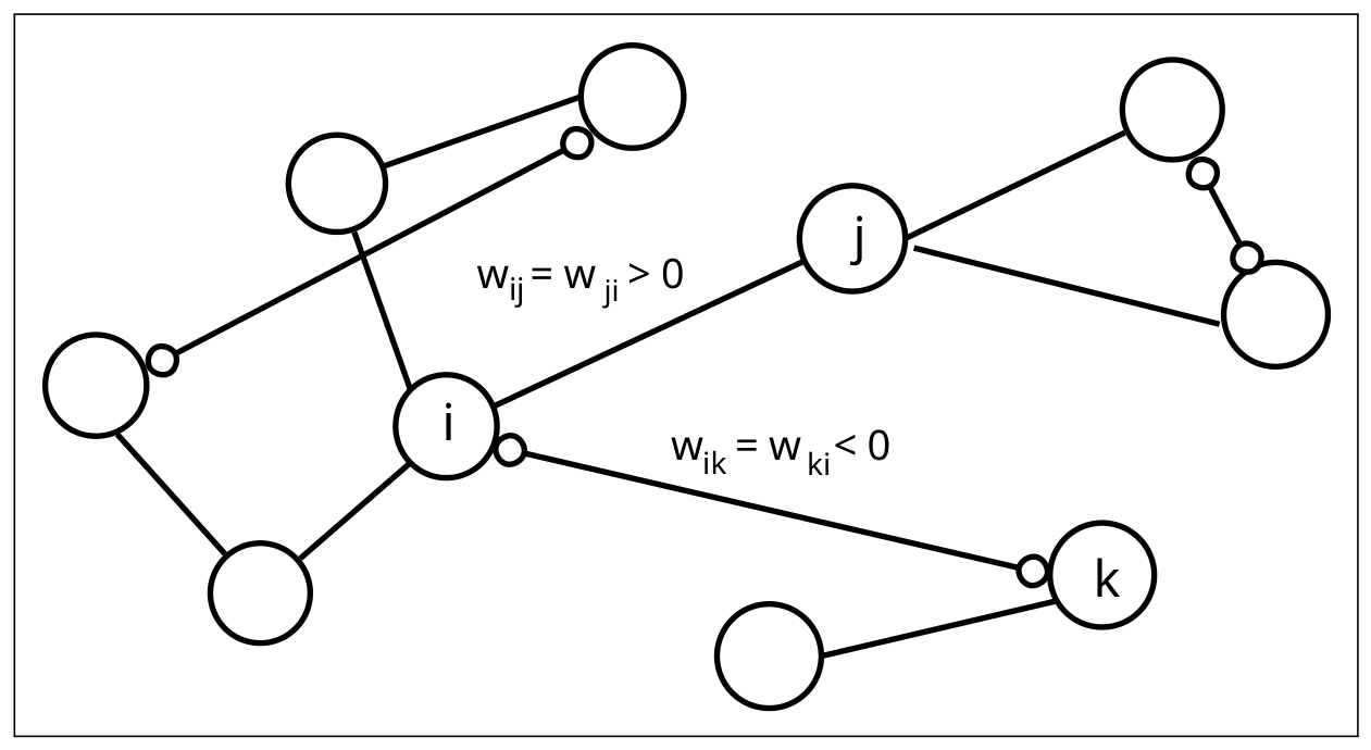
The signal from node i to node j is weighted by a coefficient . For excitatory synapses, . For inhibitory synapses, . Figure A1 illustrates these concepts on a fictional CSN.
Figure A1.
A CSN with excitatory and inhibitory synapses between nodes. Weights are symmetric and positive for excitatory synapses, symmetric and negative for inhibitory synapses.
Each coefficient is updated at each time step by an amount proportional to its contribution to neuron output. This is an instance of the Hebbian Rule.
Updating is symmetric, with . Symmetric updating favours bi-directional flows and the formation of loops, in sharp contrast to the formalisation of cognitive maps presented in Section 3. Symmetry of causal inferences runs against the prescriptions of logic, because it means that implies , leading to either , or no relation at all between them. However, it has been found that a degree of symmetry in causal inferences favours creativity and learning, in both humans and machines (see Section 4) [150].
Symmetric feedback between neurons makes the network maximise Consonance:
Consonance maximisation means that those neurons are strengthened, that represent possibilities, concepts or propositions that are coherent with one another. In general, CSNs admit one of two alternative arrangements. In general, one or a few concepts serve as tipping points that drive the systems towards one of the two possible equilibria.
Appendix B. Free Energy Minimisation
Consider a person who is trying to make sense of available information. It is sensible to assume that they will do their best to detect recurring patterns, build an internal representation of these patterns, use this representation to make predictions, and take actions that likely yield a return. This amounts to (i) tuning internal representations, and (ii) adjusting their actions with the aim of living in an environment that is sufficiently predictable to reciprocate their actions with some sort of reward. Since their actions modify their environment, this person is effectively co-creating their environmental niche.
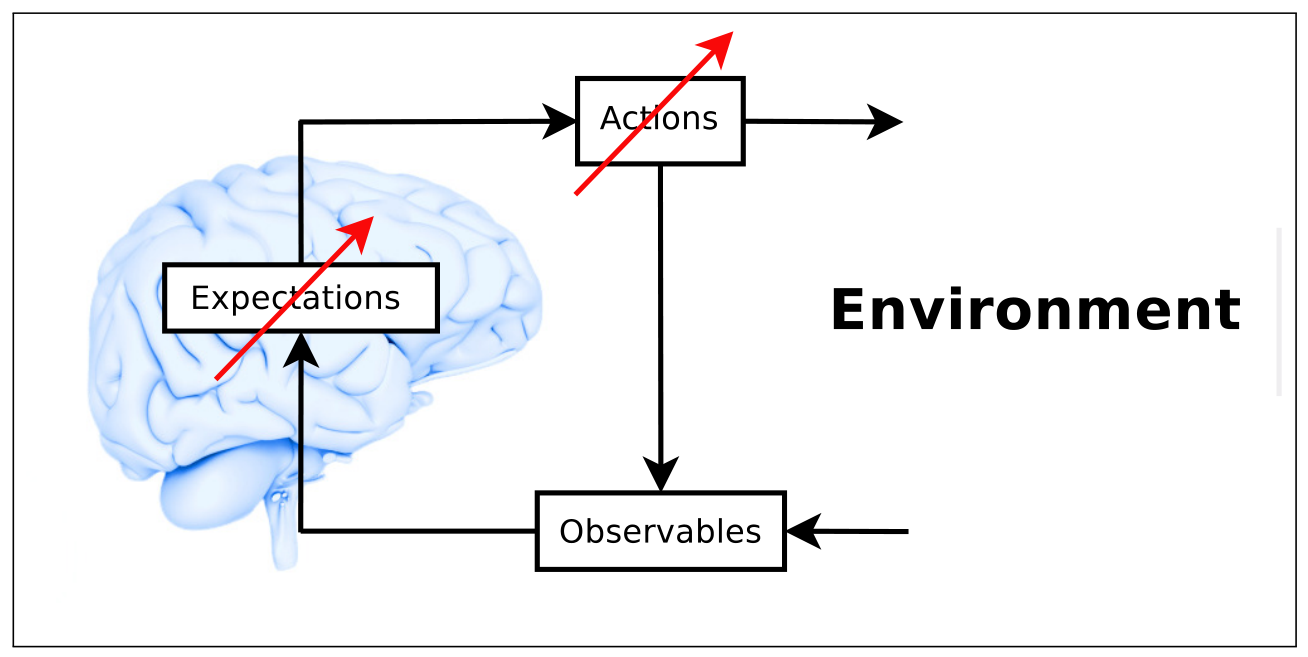
According to the Bayesian Brain Hypothesis (BBH) illustrated in Figure A2, the human brain can be assumed to employ an approximate Bayesian statistical model in order to make predictions [38,40,42]. Specifically, let denote a vector of observables, let denote a vector of internal states, and let denote a vector of actions towards the environment. Let us stipulate that M is a statistical model in the brain that generates a probability density with the aim of approximating the true probability density generated by the environment. For simplicity and without loss of generality, let us assume that is a sufficient statistics of . All vectors eventually entail derivatives of any order of the variables concerned.
Figure A2.
The brain tunes expectations and actions (red arrows) in order to increase predictability. Actions do not only impact on the environment but also on the way observables are perceived.
For this system, free energy can be expressed as:
The first term on the right side of Equation (A2) is Kullback–Leibler divergence of probability distribution Q with respect to P. The smaller , the better Q is able to track the true probability distribution P. Thus, this term must be minimised.
The second term on the right side of Equation (A2) represents the entropy of the environment as it is understood by means of inner states s. A high means that no clear pattern can be discerned among observations. Thus, provides a lower bound to free-energy minimisation, albeit patterns depend on the ability of to discern them. Therefore, this term must be minimised as well.
Notably, the presence of differentiates FEM from more naive approaches that view the brain as a mere information processor [47]. While minimising with respect to amounts to developing a good internal model of the environment, minimising with respect to amounts to constructing an environmental niche of sufficiently predictable relations. This double optimisation translates into a brain architecture designed to formulate actions that minimise prediction errors [41,43,45,169]. In this sense, FEM is a coherence-enhancing mechanism.
The relations between observables and actions are mediated by the state variables of the generative model M, which are slow-moving order parameters with respect to fast-moving variables . Thus, the fast-moving are stable within the basins of attraction specified by the but eventually modify those basins of attraction in the long run [39,170,171]. More precisely, state variables entail mental categories that classify observables ; in turn, observations eventually modify mental categories in the long run [172].
In general, Bayesian updating drives the system towards the local equilibrium of the basin of attraction it is in. In order to generate novel basins of attraction, inverse Bayesian updating is in order.
References
- Allais, M. Le comportement de l’homme rationnel devant le risque: Critique des postulats et axiomes de l’ecole americaine. Econometrica 1953, 21, 503–546. [Google Scholar] [CrossRef] [Scilit]
- Ellsberg, D. Risk, ambiguity, and the savage axioms. Q. J. Econ. 1961, 75, 643–669. [Google Scholar] [CrossRef] [Scilit]
- Tversky, A.; Shafir, E. The disjunction effect in choice under uncertainty. Psychol. Sci. 1992, 3, 305–309. [Google Scholar] [CrossRef] [Scilit]
- Tversky, A.; Kahneman, D. The framing of decisions and the psychology of choice. Science 1981, 211, 453–458. [Google Scholar] [CrossRef] [Scilit] [PubMed]
- Savage, L. The Foundations of Statistics; John Wiley & Sons: New York, NY, USA, 1954. [Google Scholar]
- Gilboa, I. Expected utility with purely subjective non-additive probabilities. J. Math. Econ. 1987, 16, 65–88. [Google Scholar] [CrossRef] [Scilit]
- Kahneman, D.; Tversky, A. Prospect theory: An analysis of decision under risk. Econometrica 1979, 47, 163–292. [Google Scholar] [CrossRef] [Scilit]
- Sarin, R.; Wakker, P. A simple axiomatization of nonadditive expected utility. Econometrica 1992, 60, 1255–1272. [Google Scholar] [CrossRef] [Scilit]
- Eliaz, K.; Ok, E.A. Indifference or indecisiveness? Choice-theoretic foundations of incomplete preferences. Games Econ. Behav. 2006, 56, 61–86. [Google Scholar] [CrossRef] [Scilit]
- Galaabaatar, T.; Karni, E. Subjective expected utility with incomplete preferences. Econometrica 2013, 81, 255–284. [Google Scholar] [CrossRef] [Scilit]
- Ok, E.A.; Ortoleva, P.; Riella, G. Incomplete preferences under uncertainty: Indecisiveness in beliefs versus tastes. Econometrica 2012, 80, 1791–1808. [Google Scholar] [CrossRef] [Scilit]
- Fischhoff, B.; Slovic, P.; Lichtenstein, S. Knowing what you want: Measuring labile values. In Cognitive Processes and Choice in Decision Behavior; Wallsten, T.S., Ed.; Erlbaum: Hillsdale, NJ, USA, 1980; Chapter VII; pp. 117–141. [Google Scholar]
- Lichtenstein, S.; Slovic, P. (Eds.) The Construction of Preference; Cambridge University Press: Cambridge, UK, 2006. [Google Scholar]
- Slovic, P. The construction of preference. Am. Psychol. 1995, 50, 364–371. [Google Scholar] [CrossRef] [Scilit]
- Slovic, P.; Griffin, D.; Tversky, A. Compatibility effects in judgment and choice. In Insights in Decision Making; Hogarth, R.M., Ed.; The University of Chicago Press: Chicago, IL, USA, 1990; Chapter I; pp. 5–27. [Google Scholar]
- Slovic, P.; Lichtenstein, S. Reversals of preference between bids and choices in gambling decisions. J. Exp. Psychol. 1971, 89, 46–55. [Google Scholar] [CrossRef] [Scilit]
- Slovic, P.; Lichtenstein, S. Response-induced reversals of preference in gambling: An extended replication in las vegas. J. Exp. Psychol. 1973, 101, 16–20. [Google Scholar] [CrossRef] [Scilit]
- Tversky, A.; Slovic, P.; Kahneman, D. The causes of preference reversal. Am. Econ. Rev. 1990, 80, 204–217. [Google Scholar]
- Bordalo, P.; Gennaioli, N.; Schleifer, A. Salience theory of choice under risk. Q. J. Econ. 2012, 127, 1243–1285. [Google Scholar] [CrossRef] [Scilit]
- Bordalo, P.; Gennaioli, N.; Schleifer, A. Salience. Annu. Rev. Econ. 2022, 14, 521–544. [Google Scholar] [CrossRef] [Scilit]
- Chen, X.; Gao, Z.; McFadden, B.R. Reveal preference reversal in consumer preference for sustainable food product. Food Qual. Prefer. 2020, 79, 103754. [Google Scholar] [CrossRef] [Scilit]
- Gluth, S.; Spektor, M.S.; Rieskamp, J. Value-based attentional capture affects multi-alternative decision making. eLife 2018, 7, e39659. [Google Scholar] [CrossRef] [Scilit] [PubMed]
- González-Vallejo, C.; Wallsten, T.S. Effects of probability mode on preference reversal. J. Exp. Psychol. Learn. Mem. Cogn. 1992, 18, 855–864. [Google Scholar] [CrossRef] [Scilit] [PubMed]
- Kim, B.E.; Seligman, D.; Kable, J.W. Preference reversals in decision making under risk are accompanied by changes in attention to different attributes. Front. Neurosci. 2012, 6, 109. [Google Scholar] [CrossRef] [Scilit] [PubMed]
- Schkade, D.A.; Johnson, E.J. Cognitive processes in preference reversals. Organ. Behav. Hum. Decis. Process. 1989, 44, 203–231. [Google Scholar] [CrossRef] [Scilit]
- Spektor, M.S.; Bhatia, S.; Gluth, S. The elusiveness of context effects in decision making. Trends Cogn. Sci. 2021, 25, 843–854. [Google Scholar] [CrossRef] [Scilit] [PubMed]
- Testsos, K.; Chater, N.; Usher, M. Salience driven value integration explains decision biases and preference reversal. Proc. Natl. Acad. Sci. USA 2012, 109, 9659–9664. [Google Scholar] [CrossRef] [Scilit] [PubMed]
- Conway, M.; Ross, M. Getting what you want by revising what you had. J. Personal. Soc. Psychol. 1984, 47, 738–748. [Google Scholar] [CrossRef] [Scilit]
- Falk, A.; Zimmermann, F. Consistency as a signal of skills. Manag. Sci. 2017, 63, 2197–2210. [Google Scholar] [CrossRef] [Scilit]
- Gawronski, B.; Strack, F. (Eds.) Cognitive Consistency: A Fundamental Principle in Social Cognition; The Guildford Press: New York, NY, USA, 2012. [Google Scholar]
- Greenwald, A.G. The totalitarian ego. Am. Psychol. 1980, 35, 603–618. [Google Scholar] [CrossRef] [Scilit]
- Kunda, Z. The case for motivated reasoning. Psychol. Bull. 1990, 108, 480–498. [Google Scholar] [CrossRef] [Scilit] [PubMed]
- Mercier, H.; Sperber, D. Why do humans reason? Arguments for an argumentative theory. Behav. Brain Sci. 2011, 34, 57–111. [Google Scholar] [CrossRef] [Scilit] [PubMed]
- Mischkowski, D.; Glöckner, A.; Lewisch, P. Information search, coherence effects, and their interplay in legal decision making. J. Econ. Psychol. 2021, 87, 102445. [Google Scholar] [CrossRef] [Scilit]
- Ross, M.; Newby-Clark, I.R. Construing the past and future. Soc. Cogn. 1998, 16, 133–150. [Google Scholar] [CrossRef] [Scilit]
- Ross, M.; Wilson, A.E. If feels like yesterday: Self-esteem, valence of personal past experiences, and judgments of subjective distance. J. Personal. Soc. Psychol. 2002, 82, 792–803. [Google Scholar] [CrossRef] [Scilit]
- Wilson, A.E.; Ross, M. From chump to champ: People’s appraisals of their earlier and present selves. J. Personal. Soc. Psychol. 2001, 80, 572–584. [Google Scholar] [CrossRef] [Scilit] [PubMed]
- Friston, K.J. The free-energy principle: A rough guide to the brain? Trends Cogn. Sci. 2009, 13, 293–301. [Google Scholar] [CrossRef] [Scilit] [PubMed]
- Friston, K.J. A free energy principle for biological systems. Entropy 2012, 14, 2100–2121. [Google Scholar] [CrossRef] [Scilit] [PubMed]
- Friston, K.J.; Daunizeau, J.; Kilner, J.; Kiebel, S. Action and behavior: A free-energy formulation. Biol. Cybern. 2010, 102, 227–260. [Google Scholar] [CrossRef] [Scilit] [PubMed]
- Friston, K.J.; Kiebel, S. Predictive coding under the free-energy principle. Philos. Trans. R. Soc. B 2009, 364, 1211–1221. [Google Scholar] [CrossRef] [Scilit] [PubMed]
- Friston, K.J.; Kilner, J.; Harrison, L. A free energy principle for the brain. J. Physiol. 2006, 100, 70–87. [Google Scholar] [CrossRef] [Scilit] [PubMed]
- Friston, K.J.; Parr, T.; de Vries, B. The graphical brain: Belief propagation and active inference. Netw. Neurosci. 2017, 1, 381–414. [Google Scholar] [CrossRef] [Scilit] [PubMed]
- Friston, K.J.; Parr, T.; Yufik, Y.; Sajid, N.; Price, C.J.; Holmes, E. Generative models, linguistic communication and active inference. Neurosci. Behav. Rev. 2020, 118, 42–64. [Google Scholar] [CrossRef] [Scilit] [PubMed]
- Kiebel, S.J.; von Kriegstein, K.; Friston, K.J. Recognizing sequences of sequences. PLoS Comput. Biol. 2009, 5, e1000464. [Google Scholar] [CrossRef] [Scilit] [PubMed]
- Park, H.-J.; Friston, K. Structural and functional brain networks: From connections to cognition. Science 2013, 342, 579–588. [Google Scholar] [CrossRef] [Scilit] [PubMed]
- Ramstead, M.J.D.; Kirchhoff, M.D.; Friston, K.J. A tale of two densities: Active inference is enactive inference. Adapt. Behav. 2020, 28, 225–239. [Google Scholar] [CrossRef] [Scilit] [PubMed]
- Friston, K.J.; Mattout, J.; Kilner, J. Action understanding and active inference. Biol. Cybern. 2011, 104, 137–160. [Google Scholar] [CrossRef] [Scilit] [PubMed]
- Albarracin, M.; Demekas, D.; Ramstead, M.J.D.; Heins, C. Epistemic communities under active inference. Entropy 2022, 24, 476. [Google Scholar] [CrossRef] [Scilit] [PubMed]
- Albarracin, M.; Constant, A.; Friston, K.J.; Ramstead, M.J.D. A variational approach to scripts. Front. Psychol. 2021, 12, 585493. [Google Scholar] [CrossRef] [Scilit] [PubMed]
- Veissière, S.P.L.; Constant, A.; Ramstead, M.J.D.; Friston, K.J.; Kirmayer, L.J. Thinking through other minds: A variational approach to cognition and culture. Behav. Brain Sci. 2020, 43, e90. [Google Scholar] [CrossRef] [Scilit] [PubMed]
- Friston, K.J. Life as we know it. J. R. Soc. Interface 2013, 10, 20130475. [Google Scholar] [CrossRef] [Scilit] [PubMed]
- Friston, K.J.; Levin, M.; Sengupta, B.; Pezzulo, G. Knowing one’s place: A free-energy approach to pattern regulation. J. R. Soc. Interface 2015, 12, 20141383. [Google Scholar] [CrossRef] [Scilit] [PubMed]
- Palacios, E.R.; Razi, A.; Parr, T.; Kirchhoff, M.; Friston, K.J. On markov blankets and hierarchicalself-organization. J. Theor. Biol. 2020, 486, 110089. [Google Scholar] [CrossRef] [Scilit] [PubMed]
- Holyoak, K.J.; Simon, D. Bidirectional reasoning in decision making by constraint satisfaction. J. Exp. Psychol. General. 1999, 128, 3–31. [Google Scholar] [CrossRef] [Scilit]
- Read, S.J.; Vanman, E.J.; Miller, L.C. Connectionism, parallel constraint satisfaction processes, and gestalt principles: (re)introducing cognitive dynamics to social psychology. Personal. Soc. Psychol. Rev. 1997, 1, 26–53. [Google Scholar] [CrossRef] [Scilit] [PubMed]
- Simon, D.; Holyoak, K.J. Structural dynamics of cognition: From consistency theories to constraint satisfaction. Personal. Soc. Psychol. Rev. 2002, 6, 283–294. [Google Scholar] [CrossRef] [Scilit] [PubMed]
- Simon, D.; Krawczyk, D.; Holyoak, K.J. Construction of preferences by constraint satisfaction. In The Construction of Preference; Lichtenstein, S., Slovic, P., Eds.; Cambridge University Press: Cambridge, UK, 2006; Chapter XII; pp. 235–245. [Google Scholar]
- Simon, D.; Snow, C.J.; Read, S.J. The redux of cognitive consistency theories: Evidence judgments by constraint satisfaction. J. Personal. Soc. Psychol. 2004, 86, 814–837. [Google Scholar] [CrossRef] [Scilit] [PubMed]
- Thagard, P. Explanatory coherence. Behav. Brain Sci. 1989, 12, 435–502. [Google Scholar] [CrossRef] [Scilit]
- Lundberg, C.G. Modeling and predicting emerging inference-based decisions in complex and ambiguous legal settings. Eur. J. Oper. Res. 2004, 153, 417–432. [Google Scholar] [CrossRef] [Scilit]
- Lundberg, C.G. Models of emerging contexts in risky and complex decision settings. Eur. J. Oper. Res. 2007, 177, 1363–1374. [Google Scholar] [CrossRef] [Scilit]
- Thagard, P. Conceptual Revolutions; Princeton University Press: Princeton, NJ, USA, 1992. [Google Scholar]
- Thagard, P. How Scientists Explain Disease; Princeton University Press: Princeton, NJ, USA, 1999. [Google Scholar]
- Bhatia, S.; Golman, R. Bidirectional constraint satisfaction in rational strategic decision making. J. Math. Psychol. 2019, 88, 48–57. [Google Scholar] [CrossRef] [Scilit]
- Chopard, B.; Raynaud, F.; Stalhandske, J. A model for the formation of beliefs and social norms based on the satisfaction problem (sat). Entropy 2025, 27, 358. [Google Scholar] [CrossRef] [Scilit] [PubMed]
- Dalege, J.; Galesic, M.; Olsson, H. Networks of beliefs: An integrative theory of individual- and social-level belief dynamics. Psychol. Rev. 2024, 132, 253–290. [Google Scholar] [CrossRef] [Scilit] [PubMed]
- Rodriguez, N.; Bollen, J.; Ahn, Y.-Y. Collective dynamics of belief evolution under cognitive coherence and social conformity. PLoS ONE 2016, 11, e0165910. [Google Scholar] [CrossRef] [Scilit] [PubMed]
- Shafer, G.R. A Mathematical Theory of Evidence; Princeton University Press: Princeton, NJ, USA, 1976. [Google Scholar]
- Shafer, G. Constructive probability. Synthese 1981, 48, 1–60. [Google Scholar] [CrossRef] [Scilit]
- Shafer, G.R.; Tversky, A. Languages and design for probability judgment. Cogn. Sci. 1985, 9, 309–339. [Google Scholar] [CrossRef] [PubMed]
- Shafer, G. Constructive decision theory. Int. J. Approx. Reason. 2016, 79, 45–62. [Google Scholar] [CrossRef] [Scilit]
- Shafer, G.R. Savage revisited. Stat. Sci. 1986, 1, 463–501. [Google Scholar] [CrossRef] [Scilit]
- Smets, P. The nature of the unnormalized beliefs encountered in the transferable belief model. In Uncertainty in Artificial Intelligence. Proceedings of the Eighth Conference; Dubois, D., Wellman, M.P., Ambrosio, B.D., Smets, P., Eds.; Morgan Kaufmann Publishers: San Mateo, CA, USA, 1992; Chapter XL; pp. 292–297. [Google Scholar]
- Smets, P.; Kennes, R. The transferable belief model. Artif. Intell. 1994, 66, 191–234. [Google Scholar] [CrossRef] [Scilit]
- Gunji, Y.-P.; Haruna, T. Concept formation and quantum-like probability from non-locality in cognition. Cogn. Comput. 2022, 14, 1328–1349. [Google Scholar] [CrossRef] [Scilit]
- Gunji, Y.-P.; Nakamura, K. Psychological origin of quantum logic: An orthomodular lattice derived from natural-born intelligence without hilbert space. BioSystems 2022, 215–216, 104649. [Google Scholar] [CrossRef] [Scilit] [PubMed]
- Liu, T.; Yu, Z.; Xiao, F.; Zhao, Y.; Aritsugi, M. A fractal-based supremum and infimum complex belief entropy in complex evidence theory. Chin. J. Aeronaut. 2025, 38, 103350. [Google Scholar] [CrossRef] [Scilit]
- Wu, K.; Xiao, F. Fractal-based belief entropy. IEEE Trans. Syst. Man. Cybern. Syst. 2025, 55, 910–924. [Google Scholar] [CrossRef] [Scilit]
- Xiao, F. Generalization of dempster-shafer theory: A complex mass function. Appl. Intell. 2020, 50, 3266–3275. [Google Scholar] [CrossRef] [Scilit]
- Jaffray, J.-Y. Bayesian updating and belief functions. IEEE Trans. Syst. Man. Cybern. 1992, 22, 1144–1152. [Google Scholar] [CrossRef] [Scilit]
- Jaffray, J.-Y.; Wakker, P. Decision making with belief functions: Compatibility and incompatibility with the sure-thing principle. J. Risk Uncertain. 1993, 7, 255–271. [Google Scholar] [CrossRef] [Scilit]
- Clark, A. Associative Engines: Connectionism, Concepts, and Representational Change; The MIT Press: Cambridge, MA, USA, 1993. [Google Scholar]
- Smolensky, P. On the proper treatment of connectionism. Behav. Brain Sci. 1988, 11, 1–74. [Google Scholar] [CrossRef] [Scilit]
- McClelland, J.L. Emergence in cognitive science. Top. Cogn. Sci. 2010, 2, 751–770. [Google Scholar] [CrossRef] [Scilit] [PubMed]
- Kohlas, J.; Monney, P.-A. Representation of evidence by hints. In Classic Works of the Dempster-Shafer Theory of Belief Functions; Yager, R.R., Liu, L., Eds.; Springer: Berlin/Heidelberg, Germany, 2008; Volume 219, pp. 665–681. [Google Scholar]
- Fioretti, G. Sherlock holmes doesn’t play dice: The mathematics of uncertain reasoning when something may happen, that you are not even able to figure out. Entropy 2025, 27, 931. [Google Scholar] [CrossRef] [Scilit] [PubMed]
- Dempster, A.P. A generalization of bayesian inference. J. R. Stat. Soc. B 1968, 30, 205–247. [Google Scholar] [CrossRef] [Scilit]
- Zadeh, L. A mathematical theory of evidence. AI Mag. 1984, 5, 81–83. [Google Scholar]
- Haenni, R. Shedding new light on zadeh’s criticism of dempster’s rule of combination. In Proceedings of the 8th International Conference on Information Fusion; IEEE: New York, NY, USA, 2005; Volume 2, pp. 879–884. [Google Scholar]
- Smets, P. Analyzing the combination of conflicting belief functions. Inf. Fusion 2007, 8, 387–412. [Google Scholar] [CrossRef] [Scilit]
- Boivin, C. Peeling Algorithm on Zadeh’s Example. 2022. Available online: https://cran.r-project.org/web/packages/dst/vignettes/Zadeh_Example.html (accessed on 10 October 2022).
- Davidson, P. Is probability theory relevant for uncertainty? A post keynesian perspective. J. Econ. Perspect. 1991, 5, 129–143. [Google Scholar] [CrossRef] [Scilit]
- Dequech, D. Uncertainty: Individuals, institutions and technology. Camb. J. Econ. 2004, 28, 365–378. [Google Scholar] [CrossRef] [Scilit]
- Dunn, S.P. Bounded rationality is not fundamental uncertainty: A post keynesian perspective. J. Post. Keynes. Econ. 2001, 23, 567–587. [Google Scholar] [CrossRef] [Scilit]
- Kay, J.; King, M. Radical Uncertainty: Decision-Making Beyond the Numbers; W.W. Norton & Company: New York, NY, USA, 2020. [Google Scholar]
- Lane, D.A.; Maxfield, R.R. Ontological uncertainty and innovation. J. Evol. Econ. 2005, 15, 3–50. [Google Scholar] [CrossRef] [Scilit]
- Runde, J. Keynesian uncertainty and the weight of arguments. Econ. Philos. 1990, 6, 275–292. [Google Scholar] [CrossRef] [Scilit]
- Altmann, P. When shared frames become contested: Environmental dynamism and capability (re)configuration as a trigger of organizational framing contests. In Uncertainty and Strategic Decision Making; Sund, K.J., Galavan, R.J., Huff, A.S., Eds.; Emerald Group Publishing Limited: Bingley, UK, 2016; Chapter II; pp. 33–56. [Google Scholar]
- Locke, K.; Golden-Biddle, K.; Feldman, M.S. Making doubt generative: Rethinking the role of doubt in the research process. Organ. Sci. 2008, 19, 907–918. [Google Scholar] [CrossRef] [Scilit]
- Steiner Sætre, A.; Van de Ven, A. Generating theory by abduction. Acad. Manag. Rev. 2021, 46, 684–701. [Google Scholar] [CrossRef] [Scilit]
- Smets, P. Belief functions. In Non-Standard Logics for Automated Reasoning; Smets, P., Ed.; Academic Press: San Diego, CA, USA, 1988; pp. 253–286. [Google Scholar]
- Smets, P. The transferable belief model and random sets. Int. J. Intell. Syst. 1992, 7, 37–46. [Google Scholar] [CrossRef] [Scilit]
- Gluth, S.; Rieskamp, J.; Büchel, C. Deciding not to decide: Computational and neural evidence for hidden behavior in sequential choice. PLoS Comput. Biol. 2013, 13, e1005476. [Google Scholar]
- Gordon, J.; Shortliffe, E.H. The dempster-shafer theory of evidence. In Readings in Uncertain Reasoning; Shafer, G., Pearl, J., Eds.; Morgan Kaufmann: San Francisco, CA, USA, 1990; Chapter 7.3; pp. 529–539. [Google Scholar]
- Shafer, G. A Mathematical Theory of Evidence turns 40. Int. J. Approx. Reason. 2016, 79, 7–25. [Google Scholar] [CrossRef] [Scilit]
- Sky tg24. COVID, Tre Anni fa Scoperto il Paziente 1 di Codogno Mattia Maestri. February 2023. Available online: https://tg24.sky.it/salute-e-benessere/2023/02/20/covid-paziente-1-codogno (accessed on 20 October 2025).
- Axelrod, R. (Ed.) Structure of Decision; Princeton University Press: Princeton, NJ, USA, 1976. [Google Scholar]
- Huff, A.S. (Ed.) Mapping Strategic Thought; John Wiley & Sons: Chichester, UK, 1990. [Google Scholar]
- Asano, M.; Basieva, I.; Khrennikov, A.; Ohya, M.; Tanaka, Y. Quantum-like dynamics of decision-making. Phys. A Stat. Mech. Its Appl. 2012, 391, 2083–2099. [Google Scholar] [CrossRef] [Scilit]
- Asano, M.; Ohya, M.; Tanaka, Y.; Basieva, I.; Khrennikov, A. Quantum-like model of brain functioning: Decision making from decoherence. J. Theor. Biol. 2011, 281, 56–64. [Google Scholar] [CrossRef] [Scilit] [PubMed]
- Gunji, Y.-P.; Nakamura, K.; Minoura, M.; Adamatzky, A. Three types of logical structure resulting from the trilemma of free will, determinism and locality. BioSystems 2020, 195, 104151. [Google Scholar] [CrossRef] [Scilit] [PubMed]
- Khrennikov, A. Open systems, quantum probability, and logic for quantum-like modeling in biology, cognition, and decision-making. Entropy 2023, 25, 886. [Google Scholar] [CrossRef] [Scilit] [PubMed]
- Busemeyer, J.R.; Shiffrin, R.M.; Wang, Z. Bayesian model comparison favors quantum over standard decision theory account of dynamic inconsistency. Decision 2015, 2, 1–12. [Google Scholar] [CrossRef] [Scilit]
- Khrennikov, A. On applicability of quantum formalism to model decision making: Can cognitive signaling be compatible with quantum theory? Entropy 2022, 24, 1592. [Google Scholar] [CrossRef] [Scilit] [PubMed]
- Pothos, E.M.; Busemeyer, J.R. Can quantum probability provide a new direction for cognitive modelling? Behav. Brain Sci. 2013, 36, 255–327. [Google Scholar] [CrossRef] [Scilit] [PubMed]
- Glöckner, A.; Betsch, T.; Schindler, N. Coherence shifts in probabilistic inference tasks. J. Behav. Decis. Mak. 2010, 23, 439–462. [Google Scholar] [CrossRef] [Scilit]
- James, G.E. Strategic Alliances: Elixirs, Poison Pills or Virtual Integration? A Longitudinal Exploration of Industry-Level Learning in Biotech. Ph.D. Thesis, Graduate School of Business, University of Colorado at Boulder, Boulder, CO, USA, 1996. [Google Scholar]
- Trofimova, I. Functional constructivism: In search of formal descriptors. Nonlinear Dyn. Psychol. Life Sci. 2017, 21, 441–474. [Google Scholar]
- Trofimova, I. Anticipatory attractors, functional neurochemistry and “throw & catch” mechanisms as illustrations of constructivism. Rev. Neurosci. 2023, 34, 737–762. [Google Scholar] [CrossRef] [Scilit] [PubMed]
- Trofimova, I. Transient nature of stable behavioural patterns, and how we can respect it. Curr. Opin. Behav. Sci. 2022, 44, 101109. [Google Scholar] [CrossRef] [Scilit]
- Gunji, Y.-P.; Shinohara, S.; Basios, V. Connecting the free energy principle with quantum cognition. Front. Neurorobot. 2022, 16, 910161. [Google Scholar] [CrossRef] [Scilit] [PubMed]
- Gunji, Y.-P.; Sonoda, K.; Basios, V. Quantum cognition based on ambiguous representation derived from a rough set approximation. BioSystems 2016, 141, 55–66. [Google Scholar] [CrossRef] [Scilit] [PubMed]
- Tito Arecchi, F. Complexity, information loss and model building: From neuro- to cognitive dynamics. In Noise and Fluctuations in Biological, Biophysical and Biomedical Systems; Bezrukov, S., Ed.; SPIE Press: Bellingham, WA, USA, 2007; Volume 6602, p. 660214. [Google Scholar]
- Gunji, Y.-P.; Shinohara, S.; Haruna, T.; Basios, V. Inverse bayesian inference as a key of consciousness featuring a macroscopic quantum logical structure. BioSystems 2017, 152, 44–65. [Google Scholar] [CrossRef] [Scilit] [PubMed]
- Arecchi, F.T. Phenomenology of consciousness: From apprehension to judgment. Nonlinear Dyn. Psychol. Life Sci. 2011, 15, 359–375. [Google Scholar]
- Gigerenzer, G.; Todd, P.M.; The ABC Research Group. Simple Heuristics That Make Us Smart; Oxford University Press: Oxford, UK, 1999. [Google Scholar]
- Gigerenzer, G.; Goldstein, D.G. Reasoning the fast and frugal way: Models of bounded rationality. Psychol. Rev. 1996, 103, 650–669. [Google Scholar] [CrossRef] [Scilit] [PubMed]
- Hutchinson, J.M.C.; Gigerenzer, G. Simple heuristics and rules of thumb: Where psychologists and behavioural biologists might meet. Behav. Process. 2005, 69, 97–124. [Google Scholar] [CrossRef] [Scilit] [PubMed]
- Mousavi, S.; Gigerenzer, G. Heuristics are tools for uncertainty. Homo Oecon. 2017, 34, 361–379. [Google Scholar] [CrossRef] [Scilit]
- Raab, M.; Gigerenzer, G. The power of simplicity: A fast-and-frugal heuristics approach to performance science. Front. Psychol. 2015, 6, 1672. [Google Scholar] [CrossRef] [Scilit] [PubMed]
- Fioretti, G. Either, or: Exploration of an emerging decision theory. IEEE Trans. Syst. Man. Cybern. C 2012, 42, 854–864. [Google Scholar] [CrossRef] [Scilit]
- Shackle, G.L.S. Decision, Order and Time in Human Affairs; Cambridge University Press: Cambridge, UK, 1961. [Google Scholar]
- Engländer, T.; Tyszka, T. Information seeking in open decision situations. Acta Psychol. 1980, 45, 169–176. [Google Scholar] [CrossRef] [Scilit]
- Montgomery, H. From cognition to action: The search for dominance in decision making. In Process and Structure in Human Decision Making; Montgomery, H., Svenson, O., Eds.; John Wiley & Sons: Chichester, UK, 1989; Chapter II; pp. 23–49. [Google Scholar]
- Montgomery, H. Decision making and action: The search for a dominance structure. In The Construction of Preference; Lichtenstein, S., Slovic, P., Eds.; Cambridge University Press: Cambridge, UK, 2006; Chapter XVIII; pp. 342–355. [Google Scholar]
- Montgomery, H.; Selart, M.; Gärling, T.; Lindberg, E. The judgment-choice discrepancy: Noncompatibility or restructuring? J. Behav. Decis. Mak. 1994, 7, 145–155. [Google Scholar] [CrossRef] [Scilit]
- Montgomery, H.; Svenson, O. A think aloud study of dominance structuring in decision processes. In Process and Structure in Human Decision Making; Montgomery, H., Svenson, O., Eds.; John Wiley & Sons: Chichester, UK, 1989; Chapter VII; pp. 135–150. [Google Scholar]
- Montgomery, H.; Willén, H. Decision making and action: The search for a good structure. In Judgment and Decision Making: Neo-Brunswikian and Process-Tracing Approaches; Juslin, P., Montgomery, H., Eds.; Lawrence Erlbaum Associates: Mahwah, NJ, USA, 1999; Chapter VIII; pp. 147–173. [Google Scholar]
- Montgomery, H. Decision rules and the search for a dominance structure: Towards a process model of decision making. In Analyzing and Aiding Decision Processes; Humphreys, P., Svenson, O., Vári, A., Eds.; North-Holland: Amsterdam, Netherlands, 1983; Volume 14, pp. 343–369. [Google Scholar]
- Tyszka, T. Contextual multiattribute decision rules. In Human Decision Making; Sjöberg, L., Tyszka, T., Wise, J.A., Eds.; Doxa: Bodafors, Sweden, 1983; pp. 243–256. [Google Scholar]
- Tyszka, T. Preselection, uncertainty of preferences, and information processing in human decision making. In Process and Structure in Human Decision Making; Montgomery, H., Svenson, O., Eds.; John Wiley & Sons: Chichester, UK, 1989; Chapter X; pp. 181–193. [Google Scholar]
- Tyszka, T. Two pairs of conflicting motives in decision making. Organ. Behav. Hum. Decis. Process. 1998, 74, 189–211. [Google Scholar] [CrossRef] [Scilit] [PubMed]
- Ariely, D.; Wallsten, T.S. Seeking subjective dominance in multidimensional space: An explanation of the asymmetric dominance effect. Organ. Behav. Hum. Decis. Process. 1995, 63, 223–232. [Google Scholar] [CrossRef] [Scilit]
- Duran-Novoa, R.; Leon-Rovira, N.; Aguayo-Tellez, H.; Said, D. Inventive problem solving based on dialectical negation, using evolutionary algorithms and triz heuristics. Comput. Ind. 2011, 62, 437–445. [Google Scholar] [CrossRef] [Scilit]
- Kadioglu, S.; Sellmann, M. Dialectic search. In Principles and Practice of Constraint Programming–CP 2009; Gent, I.P., Ed.; Springer: Lisbon, Portugal, 2009; Volume 5732, pp. 486–500. [Google Scholar]
- Ury, W. Getting Past No: Negotiating in Difficult Situations; Bantam Books: New York, NY, USA, 1993. [Google Scholar]
- Fisher, R.; Ury, W.; Patton, B. Getting to Yes: Negotiating an Agreement Without Giving in; Arrow: London, UK, 1987. [Google Scholar]
- Hattori, M.; Oaksford, M. Adaptive non-interventional heuristics for covariation detection in causal induction: Model comparison and rational analysis. Cogn. Sci. 2007, 31, 765–814. [Google Scholar] [CrossRef] [Scilit] [PubMed]
- Takahashi, T.; Nakano, M.; Shinohara, S. Cognitive symmetry: Illogical but rational bias. Symmetry Cult. Sci. 2010, 21, 275–294. [Google Scholar]
- Shinohara, S.; Manome, N.; Suzuki, K.; Chung, U.I.; Takahashi, T.; Gunji, Y.-P.; Nakajima, Y.; Mitsuyoshi, S. Extended bayesian inference incorporating symmetry bias. BioSystems 2020, 190, 104104. [Google Scholar] [CrossRef] [Scilit] [PubMed]
- Shinohara, S.; Manome, N.; Suzuki, K.; Chung, U.I.; Takahashi, T.; Okamoto, H.; Gunji, Y.-P.; Nakajima, Y.; Mitsuyoshi, S. A new method of bayesian causal inference in non-stationary environments. PLoS ONE 2020, 15, e0233559. [Google Scholar] [CrossRef] [Scilit] [PubMed]
- Shinohara, S.; Morita, D.; Hirai, H.; Kuribayashi, R.; Manome, N.; Moriyama, T.; Nakajima, Y.; Gunji, Y.-P.; Chung, U.I. Adaptive inference through bayesian and inverse bayesian inference symmetry bias in nonstationary environments. BioSystems 2026, 263, 105742. [Google Scholar] [CrossRef] [Scilit] [PubMed]
- Lewis, M.; Cristiano, V.; Lake, B.M.; Kwan, T.; Frank, M.C. The role of developmental change and linguistic experience in the mutual exclusivity effect. Cognition 2020, 198, 104191. [Google Scholar] [CrossRef] [Scilit] [PubMed]
- Malone, S.A.; Kalashnikova, M.; Davis, E.M. Is it a name or a fact? Disambiguation of reference via exclusivity and pragmatic reasoning. Cogn. Sci. 2016, 40, 2095–2107. [Google Scholar] [CrossRef] [Scilit] [PubMed]
- Gandhi, K.; Lake, B.M. Mutual exclusivity as a challenge for deep neural networks. In Advances in Neural Information Processing Systems; Larochelle, H., Ranzato, M., Hadsell, R., Balcan, M.F., Lin, H., Eds.; NeurIPS: Vancouver, BC, Canada, 2020; Volume 33. [Google Scholar]
- Ohmer, X.; Franke, M.; König, P. Mutual exclusivity in pragmatic agents. Cogn. Sci. 2021, 46, e13069. [Google Scholar] [CrossRef] [Scilit] [PubMed]
- Holyoak, K.J.; Thagard, P. Analogical mapping by constraint satisfaction. Cogn. Sci. 1989, 13, 295–355. [Google Scholar] [CrossRef] [PubMed]
- Holyoak, K.J.; Thagard, P. The analogical mind. Am. Psychol. 1997, 52, 35–44. [Google Scholar] [CrossRef] [Scilit]
- Spellman, B.A.; Holyoak, K.J. If saddam is hitler then who is george bush? Analogical mapping between systems of social roles. J. Personal. Soc. Psychol. 1992, 62, 913–933. [Google Scholar] [CrossRef] [Scilit]
- Spellman, B.A.; Holyoak, K.J. Pragmatics in analogical mapping. Cogn. Psychol. 1996, 31, 307–346. [Google Scholar] [CrossRef] [Scilit] [PubMed][Green Version]
- Steer, H.W.; Colin-Jones, D.G. Mucosal changes in gastric ulceration and their response to carbenoxolone sodium. Gut 1975, 16, 590–597. [Google Scholar] [CrossRef] [Scilit] [PubMed]
- Williams, P.M. Indeterminate probabilities. In Formal Methods in the Methodology of Empirical Sciences; Przełęcki, M., Szaniawski, K., Wójcicki, R., Malinowski, G., Eds.; Springer: Dordrecht, The Netherlands, 1976; Chapter XVI; pp. 229–246. [Google Scholar]
- Ferson, S.; Kreinovich, V.; Ginzburg, L.; Myers, D.S.; Sentz, K. Constructing Probability Boxes and Dempster-Shafer Structures; Technical Report SAND2002-4015; Sandia National Laboratories: Albuquerque, NM, USA, 2003.
- Moreira, C.; Wichert, A. Are quantum models for order effects quantum? Int. J. Theor. Phys. 2017, 56, 4029–4046. [Google Scholar] [CrossRef] [Scilit]
- Asano, M.; Ohya, M.; Khrennikov, A. Quantum-like model for decision making process in two players game. Found. Phys. 2011, 41, 538–548. [Google Scholar] [CrossRef] [Scilit]
- Pothos, E.M.; Busemeyer, J.R. Formalizing heuristics in decision making: A quantum probability perspective. Front. Psychol. 2011, 2, 289. [Google Scholar] [CrossRef] [Scilit] [PubMed]
- Thagard, P. Coherence in Thought and Action; The MIT Press: Cambridge, MA, USA, 2000. [Google Scholar]
- Friston, K.J. Hierarchical models in the brain. PLoS Comput. Biol. 2008, 4, e1000211. [Google Scholar] [CrossRef] [Scilit] [PubMed]
- Haken, H. Synergetics: An Introduction; Springer: Berlin/Heidelberger, Germany, 1983. [Google Scholar]
- Haken, H. Advanced Synergetics: Instability Hierarchies of Self-Organizing Systems and Devices; Springer: Berlin/Heidelberger, Germany, 1987. [Google Scholar]
- Tschacher, W.; Haken, H. Intentionality in non-equilibrium systems? The functional aspects of self-organized pattern formation. New Ideas Psychol. 2007, 25, 1–15. [Google Scholar] [CrossRef] [Scilit]
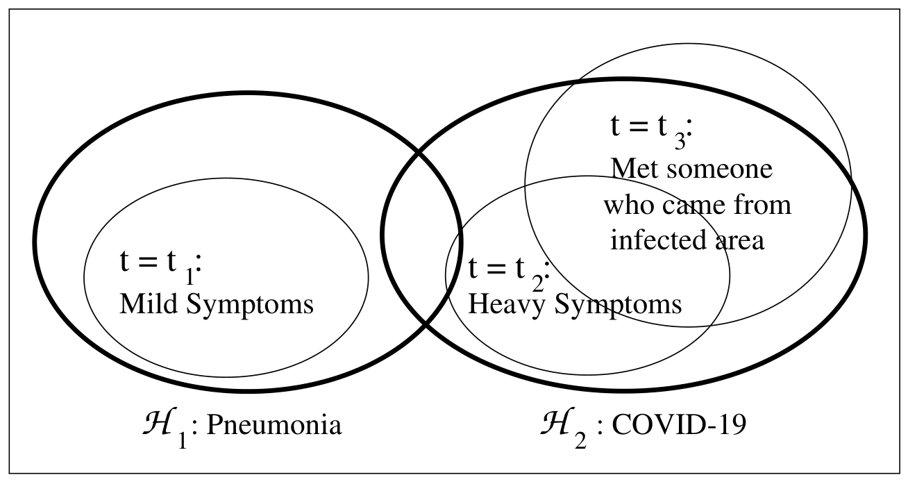
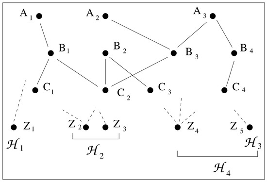
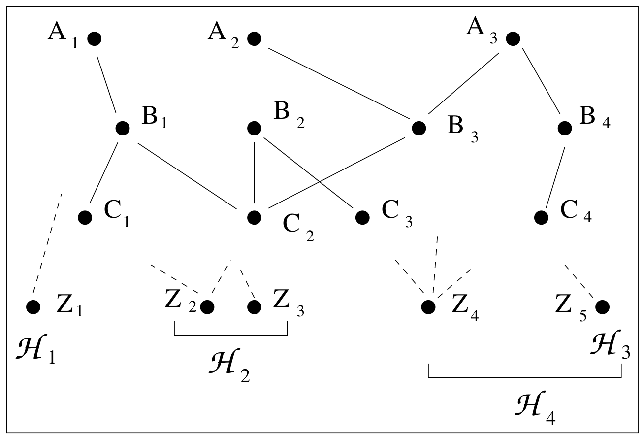
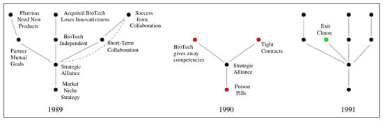
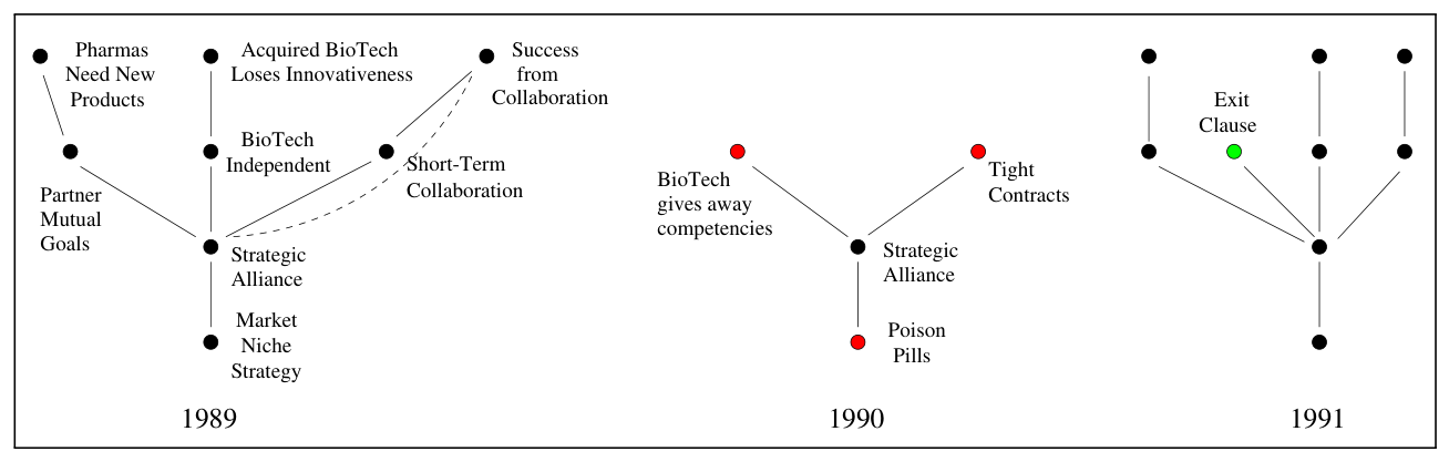
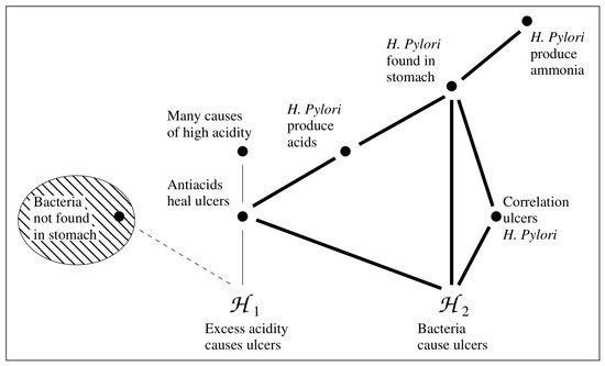
Disclaimer/Publisher’s Note: The statements, opinions and data contained in all publications are solely those of the individual author(s) and contributor(s) and not of MDPI and/or the editor(s). MDPI and/or the editor(s) disclaim responsibility for any injury to people or property resulting from any ideas, methods, instructions or products referred to in the content. |
© 2026 by the author. Licensee MDPI, Basel, Switzerland. This article is an open access article distributed under the terms and conditions of the Creative Commons Attribution (CC BY) license.