


Abstract
The impact of nonnormality on parameter estimates and model-data fit has been extensively evaluated in confirmatory factor analysis models, but comparatively less attention has been given to path models, where nonnormality may occur in different combinations across exogenous, endogenous, and mediating variables. This simulation study examined the effects of varying degrees and configurations of nonnormality on path coefficient estimation, standard errors, statistical power, and model fit under five estimation methods: maximum likelihood (ML), robust maximum likelihood (MLR), mean-adjusted maximum likelihood (MLM), mean- and variance-adjusted maximum likelihood (MLMV), and bootstrap maximum likelihood (MLB). Sample size and severity of nonnormality were systematically varied across 21 distributional configurations. Results showed that relative bias of path coefficients was generally small and approached zero as sample size increased, although coefficients involving severely nonnormal variables showed larger bias and root mean squared error when samples were small. Robust estimators (MLR, MLM, MLMV, and MLB) produced more accurate standard error estimates than ML under nonnormal conditions, with MLB showing the smallest standard error bias in the smallest samples. Statistical power increased primarily as a function of the magnitude of the path coefficient and sample size, though severe nonnormality reduced power at small sample sizes. Fit index results indicated that CFI and TLI remained very high in most conditions, even when variables were severely nonnormal. SRMR was relatively unaffected by nonnormality and sample size, whereas RMSEA was more sensitive to both factors and improved markedly with larger samples. Overall, the findings suggest that robust estimators are preferable for path analysis with nonnormal data, particularly when sample sizes are small to moderate.
1. Introduction
Path analysis has been used extensively in psychological and social behavioral sciences to examine hypothesized causal relationships among observed variables (Kline, 2023; Stage et al., 2004). It facilitates the simultaneous investigation of a system of relationships through path coefficients (standardized or unstandardized regression weights). Its primary analytical power lies in its ability to decompose the correlations between variables into three distinct components: direct effects, indirect effects, and total effects. By accounting for these mediating pathways, path analysis provides a more holistic understanding of social phenomena than traditional regression techniques.
The robustness of path model estimation is fundamentally predicated on the assumption of multivariate normality. However, in the social and behavioral sciences, true normality is rarely encountered in applied datasets (Cain et al., 2017; Jobst et al., 2022; Micceri, 1989). Consequently, a substantial body of literature within structural equation modeling (SEM) has emerged to evaluate how various estimators influence the bias and efficiency of standard errors when faced with nonnormal distributions (e.g., Du & Bentler, 2022; Maydeu-Olivares, 2017; Savalei & Rosseel, 2022), alongside comprehensive guidelines for mitigating these effects (Finney & DiStefano, 2006; Savalei & Rosseel, 2022). Despite these advancements, a significant limitation persists in the current literature: the vast majority of simulation studies focus almost exclusively on confirmatory factor analysis (CFA) models—the measurement components of SEM. While SEM assesses the relationship among latent constructs and their observed indicators, path models focus on structural relationships directly among observed variables. The specific impact of nonnormality on parameter estimates, standard errors and goodness-of-fit indices in path models with different estimators remains insufficiently investigated. Furthermore, previous research on the performance of SEM has typically examined nonnormality at the level of observed indicators, while the structural relationships themselves are often specified among continuous normal latent factors. In path analysis, exogenous variables, mediators, and endogenous variables may differ substantially in their distributional properties, with some variables exhibiting greater skewness or kurtosis. These differences may require different standard error calculations or link functions across equations, thereby further complicating model estimation and interpretation. The present study employs a multifaceted simulation design that systematically varies the degrees of nonnormality across different variable types within the path model. This allows for a more nuanced understanding of how localized nonnormality affects parameters and overall model performance. To our knowledge, no previous simulation has systematically crossed the distributional status of the exogenous, mediating, and outcome variables of a path model with the choice among the maximum likelihood (ML)-based robust estimators that applied researchers use, which is the gap addressed here.
The gold standard for estimating path models with continuous data is the ML estimator. Under the assumption of multivariate normality, ML provides parameter estimates that are both unbiased and efficient. The core mechanism of ML is an iterative optimization process designed to minimize a discrepancy function between the model implied covariance matrix and the sample covariance matrix (Ferron & Hess, 2007). Essentially, the estimator seeks the set of parameter values that maximizes the likelihood of observing the current data. This “closeness” between the observed and implied matrices is quantified by the ML fitting function (FML), which serves as the basis for the overall chi-square test of model fit. The ML fitting function () is given as:
where is the model implied covariance matrix, is the sample covariance matrix, and p and q denote the numbers of exogenous and endogenous variables, respectively. A perfectly fitting model will produce an of zero, which implies that the population and sample covariance matrices are identical (i.e., ). As described by Bollen (1989), the standard error of the estimated model parameter based on the covariance matrix is given as:
yields standard error estimates that are inaccurate when the normality assumption does not hold (Yuan & Hayashi, 2006). Other robust estimators suitable for nonnormal data have been proposed to provide corrections to the ML standard errors. These methods involve a mean adjustment or mean and variance adjustments. Some of the commonly used methods include the robust maximum likelihood (MLR) with mean corrected likelihood ratio (Asparouhov & Muthén, 2005), maximum likelihood with mean-adjusted (MLM; Satorra & Bentler, 1994), maximum likelihood with mean- and variance-adjusted (MLMV; Asparouhov & Muthén, 2010), and maximum likelihood bootstrap (MLB; Efron & Tibshirani, 1993; Yung & Bentler, 1996). The most common approach to estimating model parameters in the presence of nonnormality is to specify one of these robust correction methods (MLB, MLR, MLM, or MLMV).
The aim of this paper is to assess the extent to which estimation methods are robust to nonnormality in path analysis. Specifically, we addressed the following research questions:
- How do the degree of nonnormality, sample size, and estimation method influence the accuracy, standard errors, and statistical power of parameter estimates in path models?
- How do the degree of nonnormality, sample size, and estimation method influence the model fit indices of path models?
1.1. Literature Review
Extensive studies have been conducted on SEM to evaluate how the choice of estimators affects the standard errors of the parameter estimates with nonnormal data (e.g., Jia et al., 2026; Maydeu-Olivares, 2017; Savalei & Rosseel, 2022; Yuan et al., 2005). A review of the literature shows that several simulation studies that evaluate the impact of estimators on evaluation outcomes utilize CFA models. Maydeu-Olivares (2017) highlights that parameter estimates could be identical under different estimation methods even in the presence of nonnormality, but the standard errors vary for the different estimators. This was also echoed by Bollen (1989). Using a CFA model, Maydeu-Olivares (2017) found that MLR provided the most accurate standard errors when compared to other estimators in the presence of nonnormality. Similarly, Gao et al. (2020) investigated which estimation method results in the most accurate fit index in the presence of normality and nonnormality. They found that the MLMV provided the most accurate point estimate of root mean square error of approximation (RMSEA). While the necessity of the multivariate normality assumption is heavily emphasized in the SEM literature (e.g., Finney & DiStefano, 2006; Jobst et al., 2022), a notable disconnect persists in empirical practice. Researchers have noted that important methodological details, including assessment of distributional assumptions, treatment of nonnormality, and justification of estimation methods, are frequently underreported in SEM applications, limiting the evaluation and reproducibility of empirical findings (Boomsma, 2000; Jackson et al., 2009; Kline, 2023). Furthermore, path analysis studies often rely on maximum likelihood estimation despite its dependence on multivariate normality assumptions, which are not always explicitly evaluated or reported. This lack of methodological transparency compromises the integrity of the findings, as the resulting goodness-of-fit indices and parameter estimates become susceptible to significant bias, casting doubt on the reliability of the model’s reported structural paths.
Many empirical studies now explicitly report the normality status of their data to justify the selection of robust estimation methods. For instance, Leclerc et al. (2022) checked that the normality assumption of data was not met and utilized MLR, which employs Huber-White ‘sandwich’ standard errors to maintain validity under nonnormality. Similarly, when faced with nonnormal distributions, Bollenbach et al. (2023) used bootstrapping estimate standard errors. Furthermore, Shi et al. (2021) demonstrated the application of MLMV, which extends the Satorra–Bentler approach by incorporating a mean- and variance-adjusted correction, providing more stable p-value for chi-square testing with nonnormal data. Also, the researchers did not report the degree of nonnormality for different variables in the path analysis, such as the predictor, mediator, and outcome variables. Several options are available when nonnormality is present; however, their performance in different conditions, including different degrees of nonnormality of the variables and sample sizes, remains unknown.
1.1.1. Robust Maximum Likelihood (MLR)
In SEM and path analysis, MLR estimation has emerged as a primary solution for addressing the common issue of multivariate nonnormality in continuous data. MLR addresses nonnormality by utilizing Huber-White “sandwich” estimators to produce robust standard errors and applying the Satorra–Bentler scaling correction to the chi-square test statistic. A significant advantage of MLR over other robust methods, such as MLM, is its compatibility with full information maximum likelihood (FIML), allowing researchers to handle missing data and nonnormality simultaneously. Consequently, empirical studies often report the MLR-scaled chi-square, along with adjusted fit indices such as the CFI and RMSEA, to ensure that the observed structural relationships identified in the path model are not artifacts of distributional violations.
1.1.2. Maximum Likelihood with Mean-Adjusted (MLM)
The estimation of MLM, developed primarily by Satorra and Bentler (1988, 1994), addresses the issue of inflated chi-square statistics caused by multivariate kurtosis. Unlike standard ML, which can falsely suggest a poor model fit when data are “peaked” or skewed, MLM applies a scaling correction factor (scf) to the chi-square statistic—often referred to as the Satorra–Bentler (SB) scaled chi-square. This adjustment ensures that the mean of the test statistic’s sampling distribution matches the mean of the theoretical chi-square distribution. Additionally, MLM provides robust standard errors that remain valid even under nonnormality. A critical practical constraint of the MLM estimator is that it generally requires complete data (using listwise deletion), making it less flexible than MLR for datasets with missing values.
1.1.3. Maximum Likelihood with Mean- and Variance-Adjusted (MLMV)
MLMV estimation is a robust variant of ML designed for path models where data significantly deviate from multivariate normality, particularly in small to moderate sample sizes. While the standard MLM (Satorra–Bentler) method only adjusts the mean of the chi-square distribution, MLMV applies a more comprehensive correction that accounts for both the mean and the variance of the test statistics. This dual adjustment ensures that the model’s chi-square more closely approximates the theoretical chi-square distribution, leading to more reliable p-values and fit indices (such as CFI and TLI) when data are highly kurtotic. Despite its superior performance in maintaining the nominal Type I error rate under extreme nonnormality, MLMV, like MLM, typically requires complete cases and cannot handle missing data as flexibly as the MLR estimator. In the present study, however, all datasets were fully observed with no missing values by design.
1.1.4. Maximum Likelihood Bootstrap (MLB)
In SEM and path analysis, MLB estimation serves as a powerful nonparametric resampling technique to address violations of multivariate normality and to estimate the stability of parameter estimates. Unlike robust estimators such as MLR or MLM, which use analytical formulas to “correct” the chi-square and standard errors, the bootstrap approach empirically constructs a sampling distribution by repeatedly drawing thousands of resamples with replacement from the original dataset. This method is particularly valuable for calculating bias-corrected confidence intervals, which are essential for testing indirect effects in mediation models where the sampling distribution is often naturally skewed. Furthermore, the Bollen-Stine bootstrap is frequently utilized as a specialized form of this technique to obtain a more accurate p-value for the model’s chi-square test of fit. By transforming the data to make the null hypothesis true before resampling, Bollen-Stine provides a “scaled” assessment of model fit that is far more reliable than the standard ML chi-square when data are nonnormal. In the present study the standard nonparametric bootstrap was applied, which affects only the standard errors; the model chi-square and the fit indices derived from it are therefore identical to those obtained with ML.
1.1.5. Research Gap and Study Purpose
Building on prior SEM research, this study extends the literature by examining nonnormality within an observed-variable path model rather than primarily at the CFA indicator level. We vary nonnormality across exogenous, mediating, and outcome variables, allowing us to assess whether estimation performance for a given path is especially affected by the distributions of the variables directly involved in that path. The model also includes path coefficients ranging from 0.10 to 0.60, permitting descriptive comparisons across weaker and stronger paths. Based on prior research, we expected robust estimators to show their clearest advantages in standard error estimation under nonnormality, particularly in smaller samples, with estimator differences diminishing as sample size increased. We also examined whether the effects of nonnormality were localized to specific structural paths rather than reflecting only the overall distributional profile of the model.
2. Materials and Methods
The present study used the five-variable path model employed in previous methodological research on path models (Li, 2016; Liang et al., 2026). The model comprised two exogenous variables ( and ), two mediators ( and ), and one outcome variable (), as shown in Figure 1. This model has multiple structural paths through which nonnormality can be varied across different variable roles, while keeping the model tractable for the large simulation design. Simpler and more complex mediation or mediation-moderation structures may yield different results and should be examined in future research. The model has one degree of freedom (15 observed variances and covariances minus 14 free parameters); the only omitted path is the direct effect of X2 on M2.
Figure 1.
The population path model.
In the population model, the standardized path coefficients ranged from 0.1 to 0.6 (see Figure 1 for all the values of the parameters). The paths from Xs and Y3 had the lowest path coefficients ( and = 0.1). The correlation between the exogenous variables was set at 0.3. The residual variances for , , and were 0.336, 0.611, and 0.435, respectively, so that the variance of these variables was unity.
2.1. Simulation Factors
To evaluate the impact of nonnormality on path coefficients, standard errors, and fit indices, we conducted a Monte Carlo simulation by varying the degree of nonnormality, estimator, and sample size.
2.1.1. Severity of Nonnormality
We varied the degrees of skewness/kurtosis combinations. This study considered 21 possible combinations (configurations) that observed variables could manifest. These configurations are presented in Table 1. The three levels were normal (skewness = 0, excess kurtosis = 0), moderately nonnormal (skewness = 2, excess kurtosis = 7), and severely nonnormal (skewness = 3, excess kurtosis = 21). These levels of nonnormality were reported by Curran et al. (1996) as reflective of empirical data distributions in psychology and education. These values are widely used as benchmarks for moderate and severe nonnormality in the SEM simulation literature (e.g., Curran et al., 1996; Finney & DiStefano, 2006). Distributions of this severity are common in empirical psychological data (Cain et al., 2017). For example, Cain et al. (2017) reviewed 1567 univariate and 254 multivariate distributions from 194 studies and found 74% of univariate distributions and 68% of multivariate distributions significantly nonnormal. Configuration 1 (S1) presents a case where all the observed variables are normally distributed, whereas all observed variables are severely nonnormal in S17. The 21 configurations were formed by crossing three distributions of the outcome Y3 (normal, S1–S7; moderately nonnormal, S8–S14; severely nonnormal, S15–S21) with seven combinations of distributions for the exogenous and mediating variables (Table 1); the same structure is used to arrange the panels of all the figures presenting the results. In this way, we can examine the impact of the degree of nonnormality of Xs, Ms, and Y on different paths linking them.
Table 1.
Configuration of observed variable combinations.
2.1.2. Sample Size
Careful consideration was given to our choice of sample sizes chosen for this simulation. We note that there have been several recommendations about sample size requirements in SEM; however, there is no consensus on the minimum sample size required. Kline (2023) recommends an ideal minimum sample size of 20 for each model parameter but a less-than-ideal situation would be a sample size of 10 for each model parameter. Stage et al. (2004) noted that the accuracy and stability of path analysis decreased as sample size decreased. In this study, we considered five sample sizes (n = 50, 100, 200, 500, and 1000).
2.2. Data Generation, Analysis and Evaluation
2.2.1. Data Generation
The data were generated in R (R Core Team, 2025). Data for each configuration were generated from the population covariance matrix implied by the model in Figure 1, so that the path coefficients, the exogenous correlation, and the residual variances were identical across configurations. Each simulated dataset contained the same five variables () and the same target structural model. The 21 configurations differed only in which variables were assigned normal, moderately nonnormal, or severely nonnormal distributions. Moderate and severe nonnormality corresponded to skewness/kurtosis of 2/7 and 3/21, respectively, and were imposed using the Fleishman (1978) power transformation. sSpecifically, nonnormal data were generated as implemented in the simsem package in R. The Fleishman method uses a polynomial transformation of normally distributed variables to generate continuous variables with prespecified levels of skewness and kurtosis. For each simulation condition, the target skewness and kurtosis values were specified using the bindDist() function and incorporated into the data-generation process through the indDist argument of simsem::generate(). This procedure allowed the degree and pattern of nonnormality to be systematically manipulated across variables while maintaining the prespecified population model. All observed variables were standardized to have a mean of zero and standard deviation of one. We generated 500 datasets for each simulation condition. For proportion-based outcomes such as power and convergence, this corresponds to a maximum Monte Carlo standard error of approximately 0.022 (i.e., , which is the value at an estimated proportion of p = 0.50). For the relative bias of a path coefficient, the Monte Carlo standard error is SD()/(θ√R); for γ21 it is approximately 0.025 at n = 50 and 0.006 at n = 1000. Thus, small differences across conditions or estimators should be interpreted cautiously. The total number of data generating conditions was 105 (21 configurations × 5 sample sizes), and the total number of datasets generated was 52,500 (105 conditions × 500 replications).
2.2.2. Data Analysis and Evaluation
Parameter estimation was performed by calling Mplus (Version 8.7; Muthén & Muthén, 2021) with the X command in SAS (Version 9.4; SAS Institute, 2023) (example analysis code is provided in the Supplementary Materials). Model parameters, chi-square goodness-of-fit statistics, fit indices, and standard errors were estimated for each replication using ML, MLMV, MLR, MLM, and MLB estimation methods. Mplus default convergence criteria and default information matrices were used for all estimators; because the data were complete, no missing-data options were invoked. A replication was considered converged when Mplus terminated normally and produced parameter estimates together with standard errors; non-converged replications were excluded, and all outcome measures were computed over the converged replications only. Note that ML, MLM, MLMV, and MLR share the same point estimates and differ only in their standard errors and test statistics, and that ML and MLB share both the point estimates and the chi-square-based fit indices, because bootstrapping affects only the standard errors. In terms of MLB estimation, the ML point estimates were combined with the nonparametric (standard) bootstrap: for each dataset, 1000 bootstrap samples were drawn with replacement, the model was re-estimated in each sample, and the bootstrap standard error of each parameter was computed as the standard deviation of the estimates across the bootstrap samples; p-values for MLB were based on these standard errors. The performances of the estimations in different conditions were evaluated relative to the following criteria: relative bias of the path coefficients, root mean squared error (RMSE), coverage rate, relative standard error bias (RSEB), fit indices, and statistical power of the path coefficients. Following Hoogland and Boomsma (1998), relative bias within ±5% and relative standard error bias within ±10% were regarded as acceptable. The computation of relative bias and RMSE was as follows:
where is the rth sample estimate of the path coefficient, is the population path coefficient, and R is the number of replications.
The RSEB for each path coefficient was evaluated with the aid of the standard error bias formula provided by Bandalos and Leite (2013). The relative standard error bias was calculated as
where is the average estimated standard error and is the standard deviation of the estimates over the replications. Negative values indicate that the standard errors are underestimated; RSEB is reported as a proportion.
In addition, model fit was assessed using four primary indices: (a) the comparative fit index (CFI; Bentler, 1990), (b) the Tucker–Lewis index (TLI; Tucker & Lewis, 1973), (c) the root mean square error of approximation (RMSEA; Steiger & Lind, 1980), and (d) the standardized root mean square residual (SRMR; Bentler, 1995; Jöreskog & Sörbom, 1988). Finally, the statistical power for each path parameter was determined across the simulation conditions. Power was calculated as the proportion of replications in which the null hypothesis that a specific standardized coefficient equaled zero was correctly rejected, given a significance level of α = 0.05. Because every path coefficient in the population model is nonzero, empirical Type I error rates could not be evaluated (see Section 4.2).
3. Results
3.1. Convergence
The results of the simulation showed that all five estimation methods had high convergence rates. Convergence was achieved when a specific replication of data analysis produced parameter estimates with standard errors successfully computed. All simulation conditions estimated with ML, MLM, MLMV, and MLB achieved a 100% convergence rate (the convergence criterion is given in Section 2.2.2), whereas for some conditions estimated with MLR the proportion of converged solutions was less than 100%. As displayed in Table 2, the MLR convergence rate ranged from 93% (S12, n = 50) to 100%. It increased with sample size and was higher for configurations with normally distributed variables. Because ML, MLM, MLMV, and MLR share the same point estimates, the MLR failures occurred when the sandwich standard errors could not be computed rather than in the estimation of the parameters (see Section 4).
Table 2.
Proportion of converged solutions for the MLR estimator.
3.2. Relative Bias of Path Coefficients
Relative bias was similar for the different estimators as shown in Figure 2, which shows the relative bias of estimated path coefficient. The magnitude of in the population was 0.4 and its relative bias was generally small (between −0.02 and 0.05). When sample size reached 500 and above, the relative bias was close to zero regardless of the distribution of the variables and the estimators. However, when the sample was small (e.g., 50), relative bias was larger, especially when the endogenous variable was severely nonnormal and the exogenous variable was moderately or severely nonnormal (e.g., S3, S4, S10, S11, S17, and S18). When neither of the two variables was severely nonnormal, relative bias of was relatively smaller as shown in columns of 1, 2, and 6.
Figure 2.
Relative parameter bias for parameter. The population value is γ21 = 0.40; the y-axis is the relative bias, (mean estimate—population value)/population value, and the dashed line marks zero. Each panel is one of the 21 data configurations (S1–S21) defined in Table 1; rows correspond to the distribution of Y3 (top: normal, S1–S7; middle: moderately nonnormal, S8–S14; bottom: severely nonnormal, S15–S21) and columns to the seven combinations of distributions of X1, X2, M1, and M2. The x-axis is the sample size (n = 50, 100, 200, 500, 1000). ML = maximum likelihood; MLB = ML with bootstrap standard errors; MLM = mean-adjusted ML; MLMV = mean- and variance-adjusted ML; MLR = robust ML with sandwich standard errors. Because ML, MLM, MLMV, and MLB share identical point estimates, their lines coincide.
For a smaller structural coefficient, such as = 0.10, its relative bias as shown in Figure 3 was larger (between −0.28 and 0.50) than the path coefficient with larger magnitude, such as , when the sample size was small. The largest relative bias was observed when the exogenous variable X2 was severely nonnormal, as in S5, S12, S14, and S21; relative bias exceeded the ±5% criterion in many configurations at n ≤ 100 but was within it by n = 1000 in all configurations except S20 and S21. A similar pattern was observed for the other path coefficients, as shown in the Supplementary Materials (Figures S1–S6) of the relative bias of , , , β21, β31, and β32.
Figure 3.
Relative parameter bias for parameter. The population value is γ32 = 0.10; the y-axis is the relative bias, (mean estimate—population value)/population value, and the dashed line marks zero. Each panel is one of the 21 data configurations (S1–S21) defined in Table 1; rows correspond to the distribution of Y3 (top: normal, S1–S7; middle: moderately nonnormal, S8–S14; bottom: severely nonnormal, S15–S21) and columns to the seven combinations of distributions of X1, X2, M1, and M2. The x-axis is the sample size (n = 50, 100, 200, 500, 1000). ML = maximum likelihood; MLB = ML with bootstrap standard errors; MLM = mean-adjusted ML; MLMV = mean- and variance-adjusted ML; MLR = robust ML with sandwich standard errors. Because ML, MLM, MLMV, and MLB share identical point estimates, their lines coincide.
3.3. Root Mean Squared Error of Path Coefficients
The RMSE was similar for all the estimators as shown in Figure 4 about the RMSE of . Sample size was the major contributor to its variability. When the sample size was 1000, RMSE was around 0.05 in all different configurations of the distributions of the variables. When sample size was 50, RMSE of was between 0.13 and 0.22, majorly depending on the distributions of X1 and M2. Specifically, when X1 had normal distribution and M2 was either normally distributed (i.e., S1, S8, and S15) or moderately nonnormal (i.e., S6, S13, and S20), RMSE of was lower than in the other distributional configurations, especially when sample size was small. When X1 or M2 was severely nonnormal (S3, S5, S7, S10, S12, S14, S17, S19, and S21), the RMSE of was larger than in the other distributional configurations.
Figure 4.
Root Mean Squared Error (RMSE) for parameter. The y-axis is the root mean squared error of the estimate of γ21 across replications. Each panel is one of the 21 data configurations (S1–S21) defined in Table 1; rows correspond to the distribution of Y3 (top: normal, S1–S7; middle: moderately nonnormal, S8–S14; bottom: severely nonnormal, S15–S21) and columns to the seven combinations of distributions of X1, X2, M1, and M2. The x-axis is the sample size (n = 50, 100, 200, 500, 1000). ML = maximum likelihood; MLB = ML with bootstrap standard errors; MLM = mean-adjusted ML; MLMV = mean- and variance-adjusted ML; MLR = robust ML with sandwich standard errors. Because ML, MLM, MLMV, and MLB share identical point estimates, their lines coincide.
For , its RMSE had a similar pattern as shown in Figure 5. When the exogenous variable, X2 was severely nonnormal (S3, S5, S10, S12, S17, and S19), its RMSE was larger than the other configurations. The RMSEs of other path coefficients showed similar patterns, depending majorly on the distribution of the involved variables, especially the exogenous variable as shown in the Supplementary Materials (Figures S7–S12).
Figure 5.
Root Mean Squared Error (RMSE) for parameter. The y-axis is the root mean squared error of the estimate of γ32 across replications. Each panel is one of the 21 data configurations (S1–S21) defined in Table 1; rows correspond to the distribution of Y3 (top: normal, S1–S7; middle: moderately nonnormal, S8–S14; bottom: severely nonnormal, S15–S21) and columns to the seven combinations of distributions of X1, X2, M1, and M2. The x-axis is the sample size (n = 50, 100, 200, 500, 1000). ML = maximum likelihood; MLB = ML with bootstrap standard errors; MLM = mean-adjusted ML; MLMV = mean- and variance-adjusted ML; MLR = robust ML with sandwich standard errors. Because ML, MLM, MLMV, and MLB share identical point estimates, their lines coincide.
3.4. Relative Standard Error Bias
The results showed that the absolute values of the RSEB of were smallest when the variables involved—that is, X1 and M2—were both normally distributed (S1, S8, and S15), followed by when X1 was normally distributed and M2 was moderately nonnormal (S6, S13, and S20) and both variables were moderately nonnormal (S2, S9, and S16). The robust estimators outperformed ML when the observed variables had varying degrees of nonnormality. For distributions with some degree of nonnormality, the absolute values of standard error bias were smaller for MLB, MLM/MLMV, and MLR than for ML.
The effect of sample size was clearly noticeable. As can be seen from Figure 6 and Figure 7, as sample size increased, the standard error bias of the MLB, MLM, MLMV, and MLR approached zero, especially under configurations with nonnormal variables. Interestingly, the MLB estimator resulted in the smallest standard error bias when sample sizes were small (n = 50 and 100) and increased with the increase in sample size. Overall, results suggest that the MLB, MLR, MLM, and MLMV performed well with nonnormal data when n is relatively large (500 or 1000).
Figure 6.
Relative Standard Error Bias (RSEB) for parameter. The y-axis is the relative standard error bias, (mean estimated standard error—empirical standard deviation of the estimates)/empirical standard deviation; negative values indicate underestimated standard errors, and the dashed line marks zero. Each panel is one of the 21 data configurations (S1–S21) defined in Table 1; rows correspond to the distribution of Y3 (top: normal, S1–S7; middle: moderately nonnormal, S8–S14; bottom: severely nonnormal, S15–S21) and columns to the seven combinations of distributions of X1, X2, M1, and M2. The x-axis is the sample size (n = 50, 100, 200, 500, 1000). ML = maximum likelihood; MLB = ML with bootstrap standard errors; MLM = mean-adjusted ML; MLMV = mean- and variance-adjusted ML; MLR = robust ML with sandwich standard errors.
Figure 7.
Relative Standard Error Bias (RSEB) for parameter. The y-axis is the relative standard error bias, (mean estimated standard error—empirical standard deviation of the estimates)/empirical standard deviation; negative values indicate underestimated standard errors, and the dashed line marks zero. Each panel is one of the 21 data configurations (S1–S21) defined in Table 1; rows correspond to the distribution of Y3 (top: normal, S1–S7; middle: moderately nonnormal, S8–S14; bottom: severely nonnormal, S15–S21) and columns to the seven combinations of distributions of X1, X2, M1, and M2. The x-axis is the sample size (n = 50, 100, 200, 500, 1000). ML = maximum likelihood; MLB = ML with bootstrap standard errors; MLM = mean-adjusted ML; MLMV = mean- and variance-adjusted ML; MLR = robust ML with sandwich standard errors.
3.5. Coverage Rates
The coverage results for showed that interval accuracy generally improved with increasing sample size, but the pattern differed considerably across estimators and distributional conditions as shown in Figure 8. Under normal or relatively mild nonnormality, coverage rates for most robust estimators approached the nominal 0.95 level as sample size increased. In contrast, conventional ML consistently showed substantial undercoverage in several conditions involving severe nonnormality, particularly S3, S5, S7, S10, S12, S14, S17, S19, and S21, with coverage often declining to approximately 0.70–0.80 at larger sample sizes. The robust estimators—MLR, MLM, MLMV, and MLB—generally produced coverage rates closer to 0.95, especially at moderate to large sample sizes. Overall, these findings indicate that robust estimation substantially improved confidence interval coverage for under nonnormality, whereas increasing sample size alone did not correct the undercoverage associated with conventional ML. Compared with , coverage rates for showed less pronounced estimator differences overall, with conventional ML undercoverage generally being less severe. Nevertheless, ML still exhibited notable undercoverage in several severely nonnormal conditions, particularly S17 and S18, whereas the robust estimators maintained coverage closer to the nominal 0.95 level as shown in Figure 9.
Figure 8.
Coverage rates for parameter. The y-axis is the mean coverage rate across replications. Each panel is one of the 21 data configurations (S1–S21) defined in Table 1; rows correspond to the distribution of Y3 (top: normal, S1–S7; middle: moderately nonnormal, S8–S14; bottom: severely nonnormal, S15–S21) and columns to the seven combinations of distributions of X1, X2, M1, and M2. The x-axis is the sample size (n = 50, 100, 200, 500, 1000). ML = maximum likelihood; MLB = ML with bootstrap standard errors; MLM = mean-adjusted ML; MLMV = mean- and variance-adjusted ML; MLR = robust ML with sandwich standard errors. The dotted line indicates the coverage of 0.95.
Figure 9.
Coverage rates for parameter. The y-axis is the mean coverage rate across replications. Each panel is one of the 21 data configurations (S1–S21) defined in Table 1; rows correspond to the distribution of Y3 (top: normal, S1–S7; middle: moderately nonnormal, S8–S14; bottom: severely nonnormal, S15–S21) and columns to the seven combinations of distributions of X1, X2, M1, and M2. The x-axis is the sample size (n = 50, 100, 200, 500, 1000). ML = maximum likelihood; MLB = ML with bootstrap standard errors; MLM = mean-adjusted ML; MLMV = mean- and variance-adjusted ML; MLR = robust ML with sandwich standard errors. The dotted line indicates the coverage of 0.95.
3.6. Fit Indices
Comparative fit index. As depicted in Figure 10, overall, CFI indicated excellent model fit (CFI ≥ 0.95; Hu & Bentler, 1999) in all the conditions examined. CFI increased with sample size and was close to 1 when sample size reached 500 and 1000 regardless of the distributional configurations. CFI was close to 1 when all Xs and all Ms were normally distributed (S1, S8, and S15) or some of them were normal and others were moderately nonnormal (S6, S13, and S20), even with the smallest sample size. On the other hand, when the Xs and Ms were all severely nonnormal (S3, S10, and S17), CFI was slightly lower than in the other configurations at small sample. CFI with MLR estimation was slightly lower than values for the other estimators, and ML and MLB, which share the same chi-square-based fit indices (their lines coincide in Figure 8, Figure 9, Figure 10 and Figure 11), produced the highest CFI, followed by MLM.
Figure 10.
Comparative fit index. The y-axis is the mean comparative fit index (CFI) across replications. Each panel is one of the 21 data configurations (S1–S21) defined in Table 1; rows correspond to the distribution of Y3 (top: normal, S1–S7; middle: moderately nonnormal, S8–S14; bottom: severely nonnormal, S15–S21) and columns to the seven combinations of distributions of X1, X2, M1, and M2. The x-axis is the sample size (n = 50, 100, 200, 500, 1000). ML = maximum likelihood; MLB = ML with bootstrap standard errors; MLM = mean-adjusted ML; MLMV = mean- and variance-adjusted ML; MLR = robust ML with sandwich standard errors. Because ML and MLB share identical chi-square-based fit indices, their lines coincide.
Figure 11.
Tucker–Lewis index. The y-axis is the mean Tucker–Lewis index (TLI) across replications. Each panel is one of the 21 data configurations (S1–S21) defined in Table 1; rows correspond to the distribution of Y3 (top: normal, S1–S7; middle: moderately nonnormal, S8–S14; bottom: severely nonnormal, S15–S21) and columns to the seven combinations of distributions of X1, X2, M1, and M2. The x-axis is the sample size (n = 50, 100, 200, 500, 1000). ML = maximum likelihood; MLB = ML with bootstrap standard errors; MLM = mean-adjusted ML; MLMV = mean- and variance-adjusted ML; MLR = robust ML with sandwich standard errors. Because ML and MLB share identical chi-square-based fit indices, their lines coincide.
Tucker–Lewis index. Figure 11 displays the mean TLI estimates for the different data configurations, estimators, and sample sizes. TLI generally improved as sample size increased across all 21 configurations and all estimators. At the smallest sample size (n = 50), TLI values showed the greatest variability, ranging from approximately 0.83 to 0.96 depending on the configuration and estimator. Configurations with the most severe nonnormality, such as S3, S5, S10, S17, and S21, exhibited the lowest TLI values at small sample sizes, indicating reduced model fit in these distributional configurations. However, TLI increased steadily as the sample size grew, with most conditions reaching values above 0.95 by n = 200 and approaching 0.99 or higher at n = 500 and n = 1000. Across estimators, ML and MLB (whose fit indices are identical) produced the highest TLI values, particularly at smaller sample sizes, followed by MLM. In contrast, MLMV and MLR tended to yield slightly lower TLI values when sample sizes were small, although these differences diminished as sample size increased. By n = 500 and n = 1000, all estimators converged to nearly identical TLI values close to 1.00, indicating excellent model fit and minimal estimator-related differences. Overall, the results suggest that TLI was positively associated with sample size and that estimator choice primarily affected model fit evaluation under small-sample conditions, whereas at moderate to large sample sizes all estimators provided similarly high levels of TLI.
Standardized root mean squared residual. SRMR decreased consistently as sample size increased across all 21 configurations and estimators as shown in Figure 12, indicating improved model fit with larger samples. Overall, SRMR showed that the model fit was excellent regardless of sample size, the nonnormality of the variables, and estimators. All the five estimators produced comparable values of SRMR, and the normality status of the variables had negligible effect on SRMR.
Figure 12.
Standardized root mean squared residual (SRMR). The y-axis is the mean standardized root mean square residual across replications. Each panel is one of the 21 data configurations (S1–S21) defined in Table 1; rows correspond to the distribution of Y3 (top: normal, S1–S7; middle: moderately nonnormal, S8–S14; bottom: severely nonnormal, S15–S21) and columns to the seven combinations of distributions of X1, X2, M1, and M2. The x-axis is the sample size (n = 50, 100, 200, 500, 1000). ML = maximum likelihood; MLB = ML with bootstrap standard errors; MLM = mean-adjusted ML; MLMV = mean- and variance-adjusted ML; MLR = robust ML with sandwich standard errors. Because ML and MLB share identical chi-square-based fit indices, their lines coincide.
Root mean square error of approximation. The RMSEA results showed a clear and consistent improvement in model fit as sample size increased across all configurations and estimators as shown in Figure 13. For every condition, the mean RMSEA values decreased monotonically as sample size increased from 50 to 1000, indicating that larger samples produced estimates that more closely approximated the population model. At the smallest sample size (n = 50), RMSEA values varied substantially across configurations and estimators, ranging from approximately 0.05 in the most normal configurations (e.g., S1 and S8) to values exceeding 0.14 in the least normal configurations (e.g., S3 and S21). Notably, RMSEA values exceeding 0.14 under severe nonnormality and small sample sizes could lead to incorrect conclusions of poor model fit for a correctly specified model. As sample size increased, these differences became progressively smaller, with most RMSEA values converging to approximately 0.01–0.03 when n reached 1000. Across estimators, MLM and MLMV, which produced indistinguishable RMSEA values, generally yielded the lowest RMSEA values, particularly under smaller sample sizes, whereas MLR tended to produce the largest RMSEA values and showed the greatest sensitivity to sample size. ML and MLB, whose fit indices are identical, fell between MLR and the mean-adjusted estimators under nonnormality, and all five estimators produced nearly identical RMSEA values when the variables were normally distributed or the sample size was large.
Figure 13.
Root mean square error of approximation (RMSEA). The y-axis is the mean root mean square error of approximation across replications. Each panel is one of the 21 data configurations (S1–S21) defined in Table 1; rows correspond to the distribution of Y3 (top: normal, S1–S7; middle: moderately nonnormal, S8–S14; bottom: severely nonnormal, S15–S21) and columns to the seven combinations of distributions of X1, X2, M1, and M2. The x-axis is the sample size (n = 50, 100, 200, 500, 1000). ML = maximum likelihood; MLB = ML with bootstrap standard errors; MLM = mean-adjusted ML; MLMV = mean- and variance-adjusted ML; MLR = robust ML with sandwich standard errors. Because ML and MLB share identical chi-square-based fit indices, their lines coincide.
3.7. Power
It was worthwhile evaluating the statistical power of each path coefficient across the simulation design conditions. Using a significance level of 0.05, we evaluated the proportion of rejection of the null hypothesis that the path coefficient was zero. In this study, power rate manifested differently depending on the magnitude of the parameter of interest. When the population value of the path coefficient was relatively larger (e.g., , , and β32), their power tended to be larger than the path coefficients that were small in the population model. For brevity, of 0.40 and of 0.10 were selected as the representative large and small parameter to illustrate the impact of sample size and normality status of the variables as shown in Figure 14 and Figure 15. The statistical power results for path parameter demonstrated a strong positive relationship between sample size and power across all simulation conditions and estimators. In every configuration, power increased steadily as sample size increased from 50 to 1000, eventually approaching or reaching 1.00. At the smallest sample size (n = 50), power varied considerably across conditions, ranging from approximately 0.64 to 0.83, with the lowest values observed in the most nonnormal configurations (e.g., S3, S10, S17, and S21). As sample size increased to n = 100, power improved substantially, generally exceeding 0.80 in most conditions and estimators. By n = 200, power typically reached or exceeded the conventional 0.80 criterion, and in many configurations approached 0.95 or higher. At sample sizes of 500 and 1000, power was nearly perfect across all estimators and conditions, indicating a very high probability of correctly detecting the parameter. When the path coefficient was only 0.10 as in in the population model, the power of all the estimators was lower than for , especially when the sample size was small. As sample size increased, power increased steadily, and when n = 1000, power reached approximately 0.80–0.92 in the normal and moderately nonnormal configurations, but for the robust estimators it remained at approximately 0.55–0.75 in the most nonnormal configurations (e.g., S3, S10, S11, S17, and S18). The higher power of ML under nonnormality in Figure 15 should not be interpreted as an advantage: it is a direct consequence of the underestimated ML standard errors documented in Section 3.4 and implies inflated Type I error rates for ML under those conditions.
Figure 14.
Power of parameter. The y-axis is the empirical power, i.e., the proportion of replications in which the null hypothesis γ21 = 0 was rejected at α = 0.05 (population value 0.40). Each panel is one of the 21 data configurations (S1–S21) defined in Table 1; rows correspond to the distribution of Y3 (top: normal, S1–S7; middle: moderately nonnormal, S8–S14; bottom: severely nonnormal, S15–S21) and columns to the seven combinations of distributions of X1, X2, M1, and M2. The x-axis is the sample size (n = 50, 100, 200, 500, 1000). ML = maximum likelihood; MLB = ML with bootstrap standard errors; MLM = mean-adjusted ML; MLMV = mean- and variance-adjusted ML; MLR = robust ML with sandwich standard errors.
Figure 15.
Power of parameter. The y-axis is the empirical power, i.e., the proportion of replications in which the null hypothesis γ32 = 0 was rejected at α = 0.05 (population value 0.10). Each panel is one of the 21 data configurations (S1–S21) defined in Table 1; rows correspond to the distribution of Y3 (top: normal, S1–S7; middle: moderately nonnormal, S8–S14; bottom: severely nonnormal, S15–S21) and columns to the seven combinations of distributions of X1, X2, M1, and M2. The x-axis is the sample size (n = 50, 100, 200, 500, 1000). ML = maximum likelihood; MLB = ML with bootstrap standard errors; MLM = mean-adjusted ML; MLMV = mean- and variance-adjusted ML; MLR = robust ML with sandwich standard errors.
Across estimators, differences were most evident at smaller sample sizes. The ML and MLR estimators generally exhibited the highest power, whereas MLB tended to produce slightly lower power estimates (more conservative p-values), particularly in conditions with smaller samples; as noted above, the higher power of ML under nonnormality reflects its underestimated standard errors rather than greater sensitivity. The MLM and MLMV estimators showed intermediate performance and were often nearly indistinguishable from ML and MLR as sample size increased. Importantly, the differences among estimators diminished rapidly with increasing sample size, and all estimators achieved nearly identical power levels once the sample size reached 500 or greater. Overall, the findings indicate that statistical power for the path parameter was primarily driven by sample size, with adequate power generally achieved at sample sizes of 200 or larger and near-perfect power obtained at larger sample sizes regardless of estimator choice. For the small γ32 coefficient, by contrast, adequate power required approximately 1000 cases even under normality.
4. Discussion
A central finding of this study is that the degree of nonnormality in the observed variables substantially affected parameter estimation, standard error accuracy, model fit indices, and statistical power, particularly under small-sample conditions. Across all path coefficients, the most severe deterioration in performance occurred when the variables directly involved in a path were severely nonnormal. For example, the relative bias and RMSE of γ21 increased markedly when both X1 and M2 exhibited severe nonnormality, whereas conditions involving normally distributed or only moderately nonnormal variables showed substantially smaller bias and greater precision. Similar patterns were observed for other path coefficients, where severe nonnormality in the exogenous variable led to increased bias and RMSE. These findings suggest that the distributional characteristics of variables directly involved in a structural relation exert a stronger influence on parameter recovery than the overall distributional profile of the model.
These results are largely consistent with previous SEM research demonstrating that violations of multivariate normality can adversely affect estimation accuracy, standard errors, and model test statistics (Bollen, 1989; Curran et al., 1996; Finney & DiStefano, 2006). Prior studies have shown that skewness and kurtosis can distort covariance structures and increase sampling variability, resulting in less accurate parameter estimates and fit statistics. The present findings extend this literature by demonstrating that, in path models, the impact of nonnormality is localized primarily to the variables involved in a given structural relation rather than uniformly affecting all parameters.
Interestingly, although nonnormality affected parameter bias and precision, its impact on model fit indices was more nuanced. CFI, TLI, SRMR, and RMSEA all indicated slightly poorer fit under severe nonnormality when sample sizes were small, but these effects diminished substantially as sample size increased. This pattern is consistent with simulation studies suggesting that robust fit indices are generally resilient to moderate departures from normality, particularly when sample sizes are adequate (Hu & Bentler, 1999; Li, 2016). The consistently high CFI/TLI values should be interpreted in light of the very small degrees of freedom of the present path model. With five observed variables and few covariance-structure restrictions, the model is nearly saturated, unlike many CFA models that typically impose more restrictions and therefore have larger degrees of freedom. Thus, our results should not be interpreted as evidence that CFI/TLI are generally unaffected by nonnormality. In contrast, RMSEA is known to perform poorly in correctly specified models with very small df and small samples (Kenny et al., 2015), which may explain the elevated RMSEA values observed in some small-sample conditions.
From a practical standpoint, SRMR, which is computed from the residual correlations rather than from the chi-square statistic, was essentially unaffected by nonnormality and by the choice of estimator, and its values remained well below the conventional 0.08 cutoff in every condition. It therefore provides a more dependable descriptive index of fit for small-df path models estimated from nonnormal data in small samples. In contrast, RMSEA (and, to a lesser extent, TLI) can signal poor fit for a correctly specified model when n ≤ 100 and the variables are severely nonnormal. We therefore recommend that applied researchers not rely on RMSEA alone under these conditions and that they report SRMR alongside the chi-square-based indices.
We also caution that higher CFI/TLI or lower RMSEA for a given estimator does not necessarily indicate a more accurate estimator in this correctly specified simulation model. Differences in fit indices across estimators instead reflect their finite-sample behavior and the different corrections applied to model test statistics under nonnormality.
Among all design factors investigated, sample size emerged as the most influential determinant of estimator performance. Across parameter bias, RMSE, standard error bias, fit indices, and statistical power, performance improved consistently as sample size increased. Relative bias approached zero, RMSE decreased substantially, standard error bias diminished, fit indices improved, and power approached unity as sample size increased from 50 to 1000. The beneficial effect of larger sample sizes was especially evident under severe nonnormality. Conditions exhibiting substantial estimation difficulties at n = 50 showed dramatic improvements by n = 200 and nearly complete recovery by n = 500. For example, RMSEA values that exceeded 0.14 under severe nonnormality at n = 50 converged to approximately 0.01–0.03 when n = 1000. Similarly, statistical power for γ21 increased from approximately 0.65–0.80 at n = 50 to nearly 1.00 at n = 500 and beyond. The one important exception was the standard error bias of conventional ML, which remained at approximately −0.40 to −0.50 at n = 1000 in the most severely nonnormal configurations: larger samples do not remedy the misspecification of the normal-theory standard errors, because the ratio of the estimated to the true standard error converges to a value other than one.
These findings align closely with classical SEM theory, which emphasizes the asymptotic properties of ML estimation (Bollen, 1989; Kline, 2023). As sample size increases, parameter estimates become more efficient, standard errors become more accurate, and robust corrections become less necessary because sampling distributions increasingly approximate normality through the central limit theorem. The present results also support recommendations from simulation studies suggesting that moderate-to-large sample sizes can substantially mitigate the negative consequences of nonnormality (Boomsma & Hoogland, 2001; Wolf et al., 2013). Notably, many performance differences among estimators became negligible at sample sizes of 500 and above. This finding suggests that when large samples are available, the choice among the robust estimators becomes less critical than when sample sizes are limited.
Although sample size was the dominant factor, estimator choice influenced performance in several important ways, particularly for standard error estimation and small-sample conditions. Across parameter recovery metrics, including relative bias and RMSE, the five estimators performed remarkably similarly. All estimators produced relatively unbiased parameter estimates, especially when sample size reached 500 or greater. This finding suggests that point estimation of structural coefficients in path models is generally robust to both moderate nonnormality and estimator selection.
The primary advantage of robust estimators emerged in the estimation of standard errors. MLB, MLM, MLMV, and MLR consistently produced smaller standard error bias than conventional ML under nonnormal conditions. These findings are consistent with the extensive SEM literature showing that robust corrections improve standard error accuracy when normality assumptions are violated (Satorra & Bentler, 1994; Savalei, 2014; Yuan & Bentler, 2000). Conventional ML assumes multivariate normality and therefore tends to underestimate standard errors when skewness and kurtosis are present, whereas robust estimators incorporate corrections to account for nonnormal sampling distributions.
Among the robust estimators, MLB showed particularly favorable performance in small samples, often producing the smallest standard error bias. This finding is noteworthy because previous studies have suggested that bootstrap-based or mean-adjusted corrections may outperform asymptotic corrections under limited sample conditions (Nevitt & Hancock, 2001; Savalei, 2014). However, such findings should be interpreted as specific to the correctly specified path model and simulation conditions examined here, and may not generalize to more complex or misspecified models. In contrast, MLR exhibited slightly lower convergence rates under some conditions, particularly when severe nonnormality was combined with small sample sizes. Because ML, MLM, MLMV, and MLR share identical maximum likelihood point estimates, the lower convergence rate of MLR does not reflect the point-estimation algorithm. Rather, under our convergence criterion, the MLR failures occurred when its sandwich-type standard errors could not be computed. The sandwich estimator requires the inverse of the observed information matrix and the outer product of the casewise score vectors, and the latter can become singular or non-positive definite in small samples with heavy-tailed observations. MLM and MLMV, which rely on the expected information matrix, and conventional ML did not encounter this problem. The reduced convergence of MLR is thus a property of the computation of its standard errors in the present implementation rather than of robust corrections in general. Although convergence rates remained high overall, this finding suggests that MLR may be somewhat more sensitive to challenging estimation conditions. The fit index results also revealed subtle estimator differences. ML and MLB, which share the same chi-square-based fit indices, produced the highest TLI and CFI values, while MLM and MLMV yielded the smallest RMSEA values. MLR tended to produce slightly more conservative fit assessments, especially in small samples. However, these differences became trivial as sample size increased.
Overall, the findings are highly consistent with prior methodological research on robust estimation under nonnormality. Earlier simulation studies have shown that robust estimators such as MLM, MLMV, and MLR generally outperform conventional ML in terms of standard error accuracy and model testing when data deviate from multivariate normality (Curran et al., 1996; Finney & DiStefano, 2006; Savalei, 2014). Likewise, previous studies have documented that parameter estimates themselves are often relatively robust to nonnormality, whereas standard errors and fit statistics are considerably more sensitive (Bollen, 1989; West et al., 1995).
The present findings also reinforce the conclusions of Yuan and Bentler (2000) and Li (2016), who argued that robust corrections primarily improve inferential accuracy rather than point estimation. Furthermore, the strong influence of sample size observed in this study is consistent with longstanding evidence that asymptotic robustness improves substantially as sample size increases (Boomsma & Hoogland, 2001; Wolf et al., 2013).
4.1. Empirical Implications for Applied Researchers
Several practical recommendations emerge from these findings. First, researchers analyzing path models should pay close attention to the distributional properties of variables involved in key structural relations. Severe skewness and kurtosis can increase parameter bias, RMSE, and reduce statistical power, particularly when sample sizes are small. Routine examination of univariate and multivariate normality should therefore be considered an important preliminary step in path analysis.
Second, when data exhibit noticeable nonnormality, robust estimators should generally be preferred over conventional ML. Although all estimators produced similar parameter estimates, robust estimators consistently yielded more accurate standard errors and therefore more trustworthy hypothesis tests and confidence intervals. This recommendation is especially important when sample sizes are below approximately 200.
Third, for small samples (e.g., n ≤ 100) with moderate-to-severe nonnormality, MLB provided the most accurate standard errors while retaining the point estimates and fit indices of ML. Researchers primarily interested in accurate statistical inference may therefore benefit from selecting MLB under challenging conditions. However, researchers prioritizing statistical power should note that MLB tends to produce more conservative p-values.
Fourth, when sample sizes are moderate to large (n ≥ 500), estimator choice becomes considerably less consequential. Under these conditions, ML, MLB, MLM, MLMV, and MLR all produced highly similar parameter estimates, fit indices, and statistical power. Consequently, researchers with large samples can prioritize software availability, reporting conventions, or computational convenience when selecting an estimator.
Fifth, because adequate statistical power was generally achieved once sample size reached approximately 200 for moderate-to-large path coefficients, researchers studying nonnormal data should prioritize increasing sample size whenever possible. The results suggest that increasing sample size is often more effective than changing estimators for mitigating the adverse effects of nonnormality. In practice, robust estimation and adequate sample size should be viewed as complementary strategies for obtaining reliable results in path models with nonnormally distributed variables.
Finally, choosing among the robust estimators involves trade-offs beyond standard error accuracy. MLR is computationally efficient and supports FIML for missing data, making it a practical option when incomplete data are present. MLM and MLMV are restricted to complete-case analysis, but MLMV’s additional variance adjustment can produce more accurate chi-square-based fit statistics under severe kurtosis. MLB showed the smallest standard error bias in our smallest samples but requires repeated resampling and is therefore computationally more intensive. Researchers should therefore balance MLB’s small-sample performance against computational cost and practical considerations such as missing-data handling. The key findings and implications for applied researchers are presented in Table 3.
Table 3.
Summary of conditions associated with less favorable performance under nonnormality.
4.2. Limitations and Future Research Directions
Although the present study provides a comprehensive evaluation of estimator performance under varying degrees and configurations of nonnormality, several limitations should be acknowledged. First, the simulation was based on a relatively simple recursive path model with continuous observed variables, fixed structural relations, and no missing data. Its near-saturated structure may also have contributed to the high CFI/TLI values observed in this study. More complex SEM models, such as models containing latent variables, multiple mediators, longitudinal processes, multilevel structures, categorical indicators, or interaction effects, may respond differently to differential distributional violations of different variables in the model because measurement error, latent variable estimation, and hierarchical data introduce additional sources of sampling variability and different degrees-of-freedom profiles. Second, nonnormality was generated using specified levels of skewness and kurtosis through the Fleishman power transformation, which allowed systematic control of distributional characteristics but may not fully represent the wide variety of distributional forms observed in empirical data. Real-world data often exhibit mixtures of skewness, heavy tails, floor or ceiling effects, outliers, and heterogeneous variances that were not explicitly examined in this study. Third, because skewness and kurtosis were varied jointly, their separate effects on power cannot be identified. Similarly, differences across paths cannot be attributed solely to structural position because coefficient magnitude and variable position were not independently manipulated. Future studies should examine these factors separately. Fourth, because all structural paths in the population model were nonzero, empirical Type I error rates could not be evaluated, and Monte Carlo standard errors were computed only for proportions and for the bias of the path coefficients, not for RMSE or the fit indices; future work should include a null path and report Monte Carlo uncertainty for all outcomes. Finally, the investigation focused on five maximum likelihood-based estimators. Other estimation approaches—including Bayesian estimation, weighted least squares estimators for categorical variables, and alternative bootstrap procedures—were beyond the scope of the present study and may demonstrate different performance under severe departures from normality.
Future studies should evaluate estimator performance under additional data conditions that are frequently encountered in applied research, such as missing data, model misspecification, outliers, and mixtures of continuous and categorical variables. Examining the joint effects of these conditions with nonnormality would provide more comprehensive guidance for empirical researchers. Finally, future research should compare the ML-based estimators examined here with Bayesian estimation methods and newer robust estimation procedures, particularly in small samples where asymptotic assumptions are less likely to hold. Such work would contribute to a more complete understanding of the strengths and limitations of competing estimation approaches and further inform best practices for analyzing path models with nonnormally distributed data.
5. Conclusions
This study compared five maximum likelihood-based estimators (ML, MLR, MLM, MLMV, and MLB) for a five-variable path model under 21 configurations of nonnormality and five sample sizes (52,500 simulated datasets). Four conclusions follow. First, point estimates of the path coefficients were largely unaffected by nonnormality and were identical across estimators; the bias that did occur was localized, appearing in small samples for coefficients whose own variables were severely nonnormal, and was proportionally larger for small coefficients. Second, the principal cost of nonnormality was in the standard errors: conventional ML underestimated them, in the most severely nonnormal configurations by 40–50%, and this underestimation did not diminish as sample size increased. The four robust estimators corrected most of this bias, with MLB performing best at n = 50 and 100 and all four reaching acceptable accuracy (|RSEB| < 0.10) in most configurations by n = 200–500. Third, model fit indices behaved differently: SRMR was insensitive to nonnormality and estimator, CFI remained above 0.95 throughout, whereas TLI and especially RMSEA could indicate poor fit for the correctly specified model when n ≤ 100 and the variables were severely nonnormal, a pattern attributable to the very small degrees of freedom of the model. Fourth, statistical power depended primarily on effect size and sample size; adequate power for a moderate coefficient (0.40) required about n = 200, whereas for a small coefficient (0.10) it required about n = 1000. The apparently higher power of ML under nonnormality was an artifact of its underestimated standard errors. For applied researchers analyzing path models, these findings support a simple decision rule: (a) examine the distributions of the variables involved in the structural relations of interest; (b) when notable nonnormality is present, use a robust estimator regardless of sample size—MLB when n ≤ 100 and standard error accuracy is the priority, and otherwise MLR, MLM, or MLMV, with MLR offering the practical advantage of full-information estimation with incomplete data; (c) report SRMR alongside RMSEA and interpret RMSEA cautiously in small-df models with small samples; and (d) plan sample size according to the smallest effect of interest, because increasing sample size improves every outcome examined here except the standard error bias of conventional ML.
Supplementary Materials
The following supporting information can be downloaded at: https://www.mdpi.com/article/10.3390/psycholint8040065/s1. Figure S1. Relative parameter bias for parameter. Figure S2. Relative parameter bias for parameter. Figure S3. Relative parameter bias for parameter. Figure S4. Relative parameter bias for parameter. Figure S5. Relative parameter bias or parameter. Figure S6. Relative parameter bias for parameter. Figure S7. Root Mean Squared Error (RMSE) for parameter. Figure S8. Root Mean Squared Error (RMSE) for parameter. Figure S9. Root Mean Squared Error (RMSE) for parameter. Figure S10. Root Mean Squared Error (RMSE) for parameter. Figure S11. Root Mean Squared Error (RMSE) for parameter. Figure S12. Root Mean Squared Error (RMSE) for parameter. Figure S13. Relative Standard Error Bias (RSEB) for parameter. Figure S14. Relative Standard Error Bias (RSEB) for parameter. Figure S15. Relative Standard Error Bias (RSEB) for parameter. Figure S16. Relative Standard Error Bias (RSEB) for parameter. Figure S17. Relative Standard Error Bias (RSEB) for parameter. Figure S18. Relative Standard Error Bias (RSEB) for parameter. Figure S19. Coverage rate for parameter. Figure S20. Coverage rate for parameter. Figure S21. Coverage rate for parameter. Figure S22. Coverage rate for parameter. Figure S23. Coverage rate for parameter. Figure S24. Coverage rate for parameter. Figure S25. Statistical power for parameter. Figure S26. Statistical power for parameter. Figure S27. Statistical power for parameter. Figure S28. Statistical Power for parameter. Figure S29. Statistical power for parameter. Figure S30. Statistical power for parameter. Code S1: Example R Data Generation Syntax of S10 (Xs and Ms Are Severely Nonnormal and Y is Moderately Nonnormal. Code S2: Example SAS Syntax Code of Model Analysis and Mplus Input.
Author Contributions
Conceptualization, C.C. and X.L.; methodology, C.C., X.L., W.-J.L. and N.C.E.; software, C.C. and N.C.E.; validation, C.C., X.L., W.-J.L. and N.C.E.; formal analysis, C.C. and N.C.E.; investigation, C.C. and N.C.E.; resources, C.C. and N.C.E.; data curation, C.C. and N.C.E.; writing—original draft preparation, C.C. and N.C.E.; writing—review and editing, C.C., X.L., W.-J.L., J.L. and N.C.E.; visualization, C.C. and N.C.E.; supervision, C.C., X.L. and W.-J.L.; project administration C.C. All authors have read and agreed to the published version of the manuscript.
Funding
This research received no external funding.
Institutional Review Board Statement
Not applicable.
Informed Consent Statement
Not applicable.
Data Availability Statement
The simulation code and the summary results for all conditions are available at https://osf.io/594xq/overview (accessed on 24 June 2026).
Conflicts of Interest
The authors declare no conflicts of interest.
References
- Asparouhov, T., & Muthén, B. (2005). Multivariate statistical modeling with survey data. Mplus technical report. Available online: https://www.statmodel.com/download/2005FCSM.pdf (accessed on 24 June 2026).
- Asparouhov, T., & Muthén, B. (2010). Simple second order chi-square correction. Mplus technical report. Available online: https://www.statmodel.com/download/WLSMV_new_chi21 (accessed on 24 June 2026).
- Bandalos, D. L., & Leite, W. (2013). Use of monte Carlo studies in structural equation modeling research. In G. R. Hancock, & R. O. Mueller (Eds.), Structural equation modeling: A second course (2nd ed., pp. 625–666). Information Age Publishing. [Google Scholar]
- Bentler, P. M. (1990). Comparative fit indexes in structural models. Psychological Bulletin, 107(2), 238–246. [Google Scholar] [CrossRef] [Scilit] [PubMed]
- Bentler, P. M. (1995). EQS structural equations program manual (Version 5.0). Multivariate Software. [Google Scholar]
- Bollen, K. A. (1989). Structural equations with latent variables. John Wiley & Sons. [Google Scholar]
- Bollenbach, L., Niermann, C., Schmitz, J., & Kanning, M. (2023). Social participation in the city: Exploring the moderating effect of walkability on the associations between active mobility, neighborhood perceptions, and social activities in urban adults. BMC Public Health, 23, 2450. [Google Scholar] [CrossRef] [Scilit] [PubMed]
- Boomsma, A. (2000). Reporting analyses of covariance structures. Structural Equation Modeling, 7(3), 461–483. [Google Scholar] [CrossRef] [Scilit] [PubMed]
- Boomsma, A., & Hoogland, J. J. (2001). The robustness of LISREL modeling revisited. In R. Cudeck, S. du Toit, & D. Sörbom (Eds.), Structural equation models: Present and future—A festschrift in honor of Karl Jöreskog (pp. 139–168). Scientific Software International. [Google Scholar]
- Cain, M. K., Zhang, Z., & Yuan, K.-H. (2017). Univariate and multivariate skewness and kurtosis for measuring nonnormality: Prevalence, influence and estimation. Behavior Research Methods, 49(5), 1716–1735. [Google Scholar] [CrossRef] [Scilit] [PubMed]
- Curran, P. J., West, S. G., & Finch, J. F. (1996). The robustness of test statistics to nonnormality and specification error in confirmatory factor analysis. Psychological Methods, 1(1), 16–29. [Google Scholar] [CrossRef]
- Du, H., & Bentler, P. M. (2022). 40-year old unbiased distribution free estimator reliably improves SEM statistics for nonnormal data. Structural Equation Modeling: A Multidisciplinary Journal, 29(6), 872–887. [Google Scholar] [CrossRef] [Scilit]
- Efron, B., & Tibshirani, R. J. (1993). An introduction to the bootstrap. Chapman & Hall. [Google Scholar]
- Ferron, J. M., & Hess, M. R. (2007). Estimation in SEM: A concrete example. Journal of Educational and Behavioral Statistics, 32(1), 110–120. [Google Scholar] [CrossRef] [Scilit]
- Finney, S. J., & DiStefano, C. (2006). Non-normal and categorical data in structural equation modeling. In G. R. Hancock, & R. O. Mueller (Eds.), Structural equation modeling: A second course (pp. 269–314). Information Age Publishing. [Google Scholar]
- Fleishman, A. I. (1978). A method for simulating non-normal distributions. Psychometrika, 43(4), 521–532. [Google Scholar] [CrossRef] [Scilit]
- Gao, C., Shi, D., & Maydeu-Olivares, A. (2020). Estimating the maximum likelihood root mean square error of approximation (RMSEA) with non-normal data: A monte Carlo study. Structural Equation Modeling: A Multidisciplinary Journal, 27(2), 192–201. [Google Scholar] [CrossRef] [Scilit]
- Hoogland, J. J., & Boomsma, A. (1998). Robustness studies in covariance structure modeling: An overview and a meta-analysis. Sociological Methods & Research, 26(3), 329–367. [Google Scholar] [CrossRef] [Scilit]
- Hu, L.-T., & Bentler, P. M. (1999). Cutoff criteria for fit indexes in covariance structure analysis: Conventional criteria versus new alternatives. Structural Equation Modeling: A Multidisciplinary Journal, 6(1), 1–55. [Google Scholar] [CrossRef] [Scilit]
- Jackson, D. L., Gillaspy, J. A., & Purc-Stephenson, R. (2009). Reporting practices in confirmatory factor analysis: An overview and some recommendations. Psychological Methods, 14(1), 6–23. [Google Scholar] [CrossRef] [Scilit] [PubMed]
- Jia, F., Jorgensen, T., & Wu, W. (2026). Obtaining robust practical fit indices with multiply imputed nonnormal data in structural equation modeling. Behavor Research Methods, 58, 113. [Google Scholar] [CrossRef] [Scilit] [PubMed]
- Jobst, L. J., Auerswald, M., & Moshagen, M. (2022). The effect of latent and error non-normality on corrections to the test statistic in structural equation modeling. Behavior Research Methods, 54, 2351–2363. [Google Scholar] [CrossRef] [Scilit] [PubMed]
- Jöreskog, K. G., & Sörbom, D. (1988). LISREL 7: A guide to the program and applications (2nd ed.). SPSS. [Google Scholar]
- Kenny, D. A., Kaniskan, B., & McCoach, D. B. (2015). The performance of RMSEA in models with small degrees of freedom. Sociological Methods & Research, 44(3), 486–507. [Google Scholar] [CrossRef] [Scilit]
- Kline, R. B. (2023). Principles and practice of structural equation modeling (5th ed.). Guilford Press. [Google Scholar]
- Leclerc, M.-E., Lafontaine, M.-F., Brassard, A., & Péloquin, K. (2022). Exploring insecure romantic attachment and justifications for the use of intimate partner psychological aggression in couples. Journal of Interpersonal Violence, 37(21–22), NP21070–NP21091. [Google Scholar] [CrossRef] [Scilit] [PubMed]
- Li, C.-H. (2016). The performance of ML, DWLS, and ULS estimation with robust corrections in structural equation models with ordinal variables. Psychological Methods, 21(3), 369–387. [Google Scholar] [CrossRef] [Scilit] [PubMed]
- Liang, X., Castro, P., Cao, C., & Lo, W.-J. (2026). Path analysis with mixed-scale variables: Categorical ML, least squares, and bayesian estimations. Educational and Psychological Measurement, 86(3), 525–552. [Google Scholar] [CrossRef] [Scilit] [PubMed]
- Maydeu-Olivares, A. (2017). Maximum likelihood estimation of structural equation models for continuous data: Standard errors and goodness of fit. Structural Equation Modeling: A Multidisciplinary Journal, 24(3), 383–458. [Google Scholar] [CrossRef] [Scilit]
- Micceri, T. (1989). The unicorn, the normal curve, and other improbable creatures. Psychological Bulletin, 105(1), 156–166. [Google Scholar] [CrossRef]
- Muthén, L. K., & Muthén, B. O. (2021). Mplus user’s guide (Version 8.7) [Computer software]. Muthén & Muthén. [Google Scholar]
- Nevitt, J., & Hancock, G. R. (2001). Performance of bootstrapping approaches to model test statistics and parameter standard error estimation in structural equation modeling. Structural Equation Modeling: A Multidisciplinary Journal, 8(3), 353–377. [Google Scholar] [CrossRef] [Scilit] [PubMed]
- R Core Team. (2025). R: A language and environment for statistical computing (Version 4.5.0) [Computer software]. R Foundation for Statistical Computing. Available online: https://www.R-project.org/ (accessed on 2 February 2026).
- SAS Institute. (2023). SAS/STAT software (Version 9.4) [Computer software]. SAS Institute Inc. [Google Scholar]
- Satorra, A., & Bentler, P. M. (1988). Scaling corrections for chi-square statistics in covariance structure analysis. In Proceedings of the American statistical association, business and economic statistics section (pp. 308–313). American Statistical Association. [Google Scholar]
- Satorra, A., & Bentler, P. M. (1994). Corrections to test statistics and standard errors in covariance structure analysis. In A. von Eye, & C. C. Clogg (Eds.), Latent variables analysis: Applications for developmental research (pp. 399–419). Sage Publications, Inc. [Google Scholar]
- Savalei, V. (2014). Understanding robust corrections in structural equation modeling. Structural Equation Modeling: A Multidisciplinary Journal, 21(1), 149–160. [Google Scholar] [CrossRef] [Scilit]
- Savalei, V., & Rosseel, Y. (2022). Computational options for standard errors and test statistics with incomplete normal and nonnormal data in SEM. Structural Equation Modeling: A Multidisciplinary Journal, 29(2), 163–181. [Google Scholar] [CrossRef] [Scilit]
- Shi, D., DiStefano, C., Zheng, X., Liu, R., & Jiang, Z. (2021). Fitting latent growth models with small sample sizes and non-normal missing data. International Journal of Behavioral Development, 45(2), 179–192. [Google Scholar] [CrossRef] [Scilit] [PubMed]
- Stage, F. K., Carter, H. C., & Nora, A. (2004). Path analysis: An introduction and analysis of a decade of research. The Journal of Educational Research, 98(1), 5–13. [Google Scholar] [CrossRef] [Scilit]
- Steiger, J. H., & Lind, J. C. (1980, May 30). Statistically based tests for the number of common factors. Paper Presented at the Annual Meeting of the Psychometric Society, Iowa City, IA, USA. [Google Scholar]
- Tucker, L. R., & Lewis, C. (1973). A reliability coefficient for maximum likelihood factor analysis. Psychometrika, 38(1), 1–10. [Google Scholar] [CrossRef] [Scilit]
- West, S. G., Finch, J. F., & Curran, P. J. (1995). Structural equation models with nonnormal variables: Problems and remedies. In R. H. Hoyle (Ed.), Structural equation modeling: Concepts, issues, and applications (pp. 56–75). Sage. [Google Scholar]
- Wolf, E. J., Harrington, K. M., Clark, S. L., & Miller, M. W. (2013). Sample size requirements for structural equation models: An evaluation of power, bias, and solution propriety. Educational and Psychological Measurement, 73(6), 913–934. [Google Scholar] [CrossRef] [Scilit] [PubMed]
- Yuan, K.-H., & Bentler, P. M. (2000). Three likelihood-based methods for mean and covariance structure analysis with nonnormal missing data. Sociological Methodology, 30(1), 165–200. [Google Scholar] [CrossRef] [Scilit]
- Yuan, K.-H., Bentler, P. M., & Zhang, W. (2005). The effect of skewness and kurtosis on mean and covariance structure analysis: The univariate case and its multivariate implication. Sociological Methods & Research, 34(2), 240–258. [Google Scholar] [CrossRef] [Scilit]
- Yuan, K.-H., & Hayashi, K. (2006). Standard errors in covariance structure models: Asymptotics versus bootstrap. British Journal of Mathematical and Statistical Psychology, 59(2), 397–417. [Google Scholar] [CrossRef] [Scilit] [PubMed]
- Yung, Y.-F., & Bentler, P. M. (1996). Bootstrapping techniques in analysis of mean and covariance structures. In G. A. Marcoulides, & R. E. Schumacker (Eds.), Advanced structural equation modeling: Issues and techniques (pp. 195–226). Lawrence Erlbaum Associates, Inc. [Google Scholar]
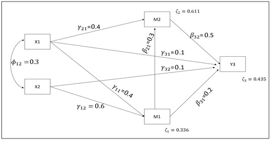
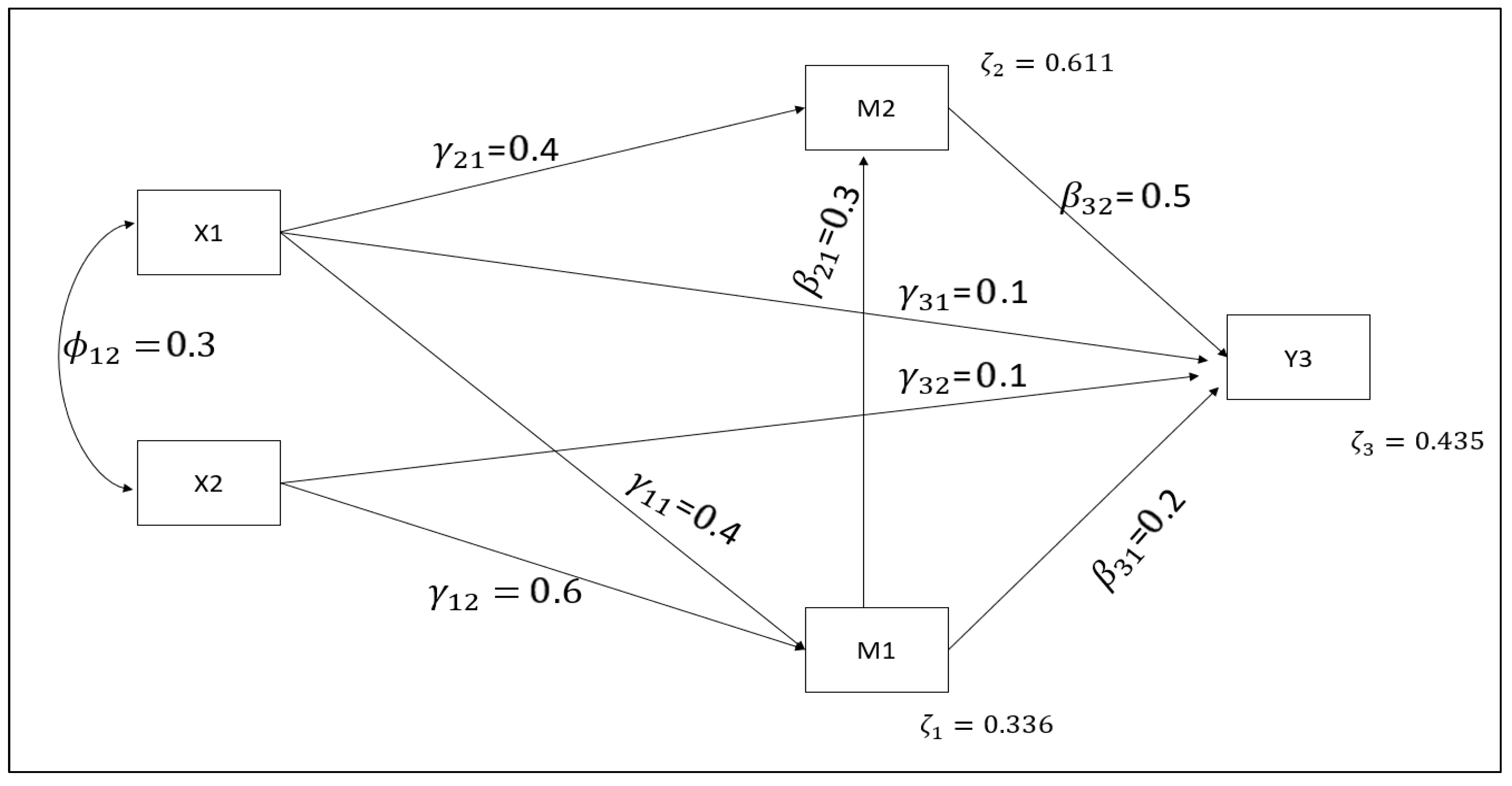
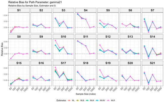
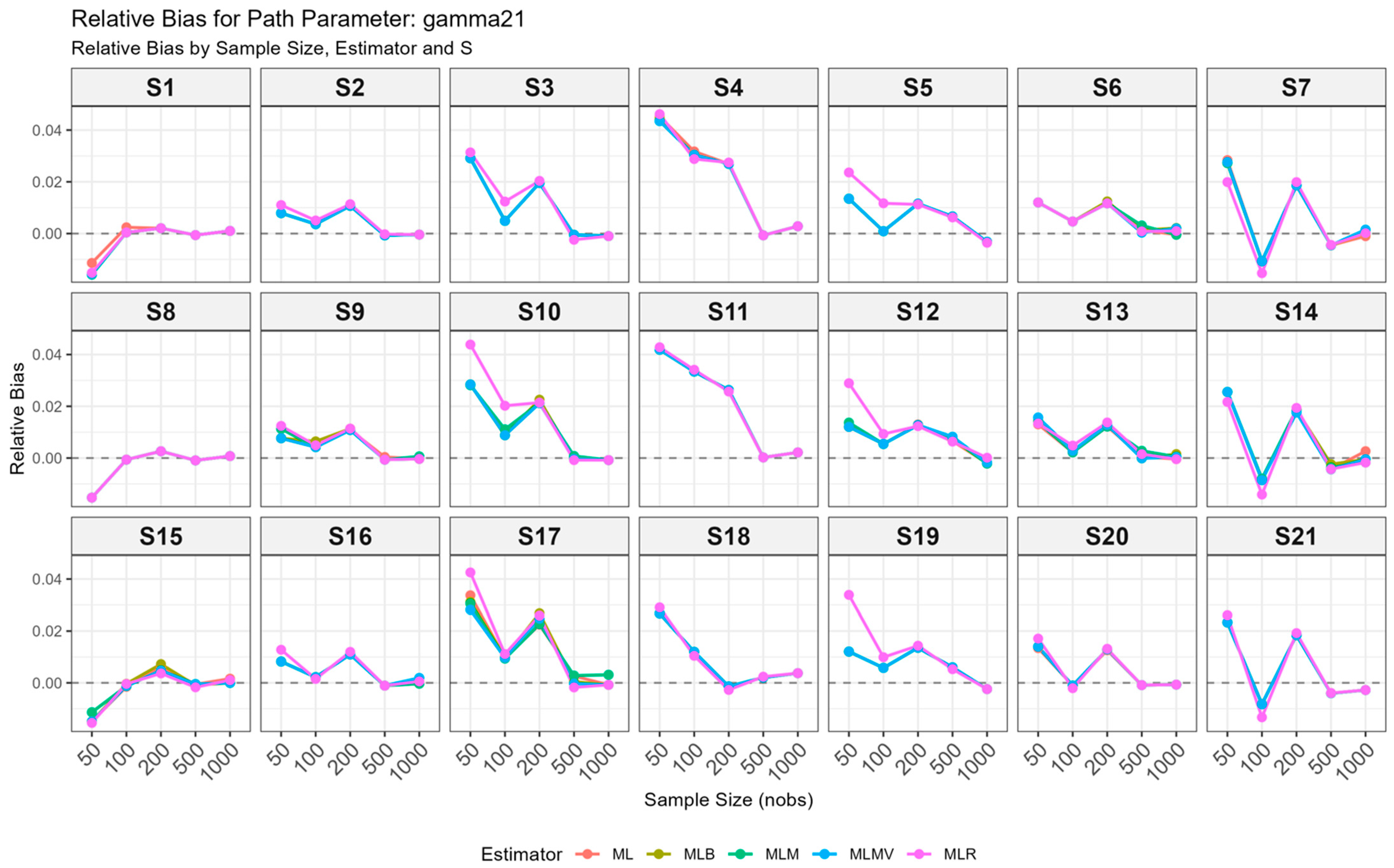
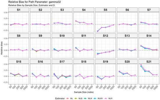
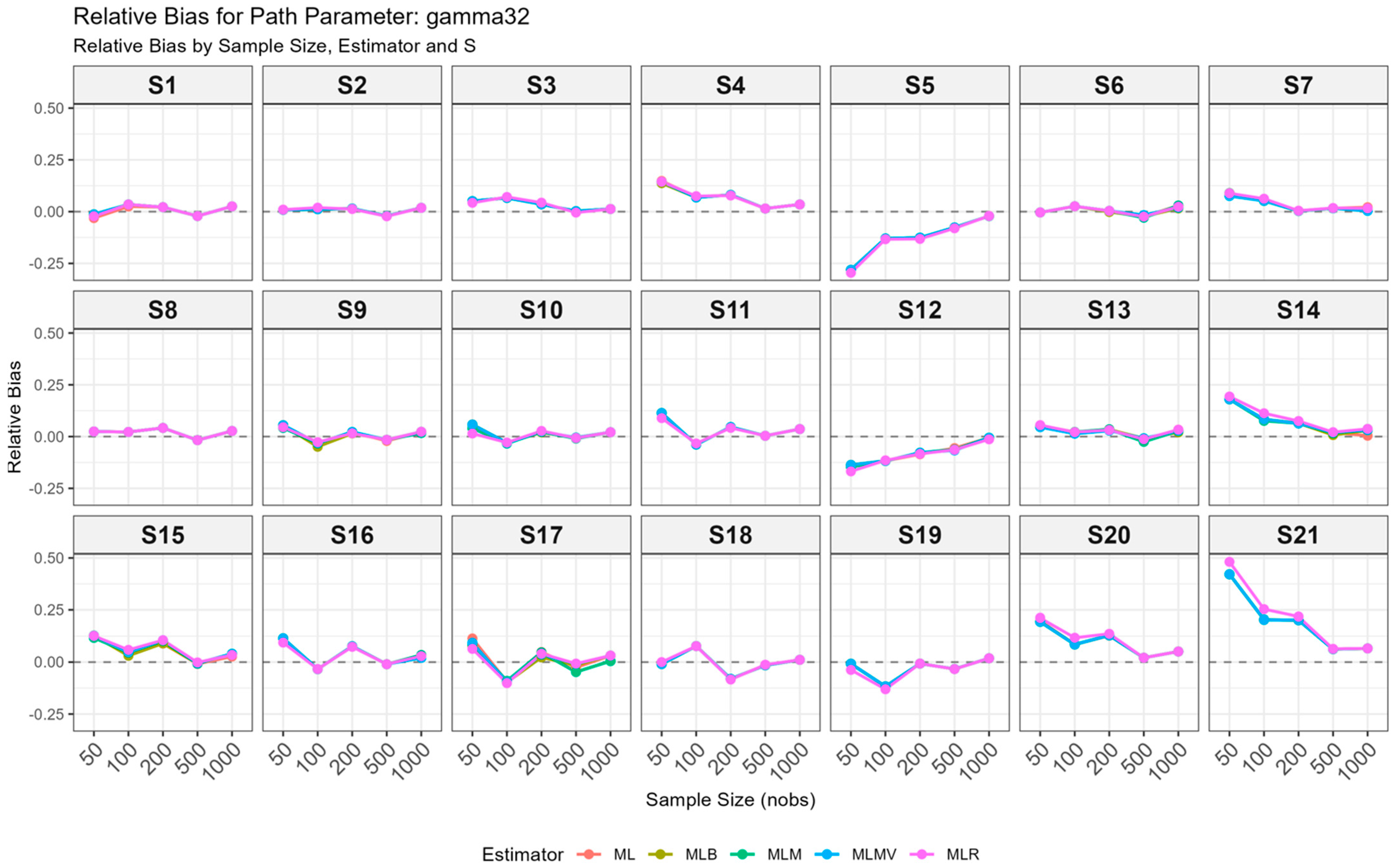
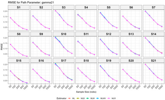
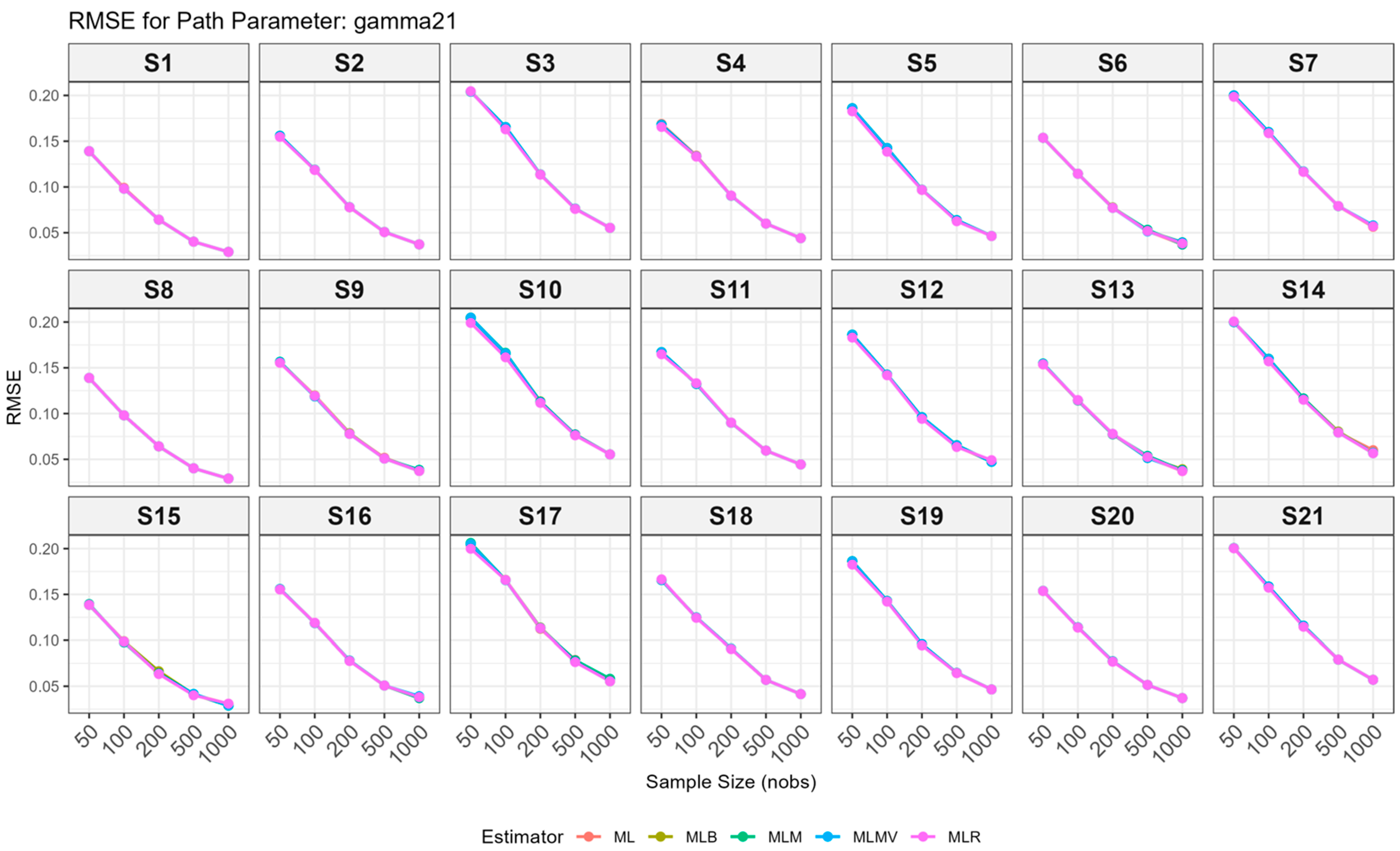
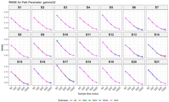
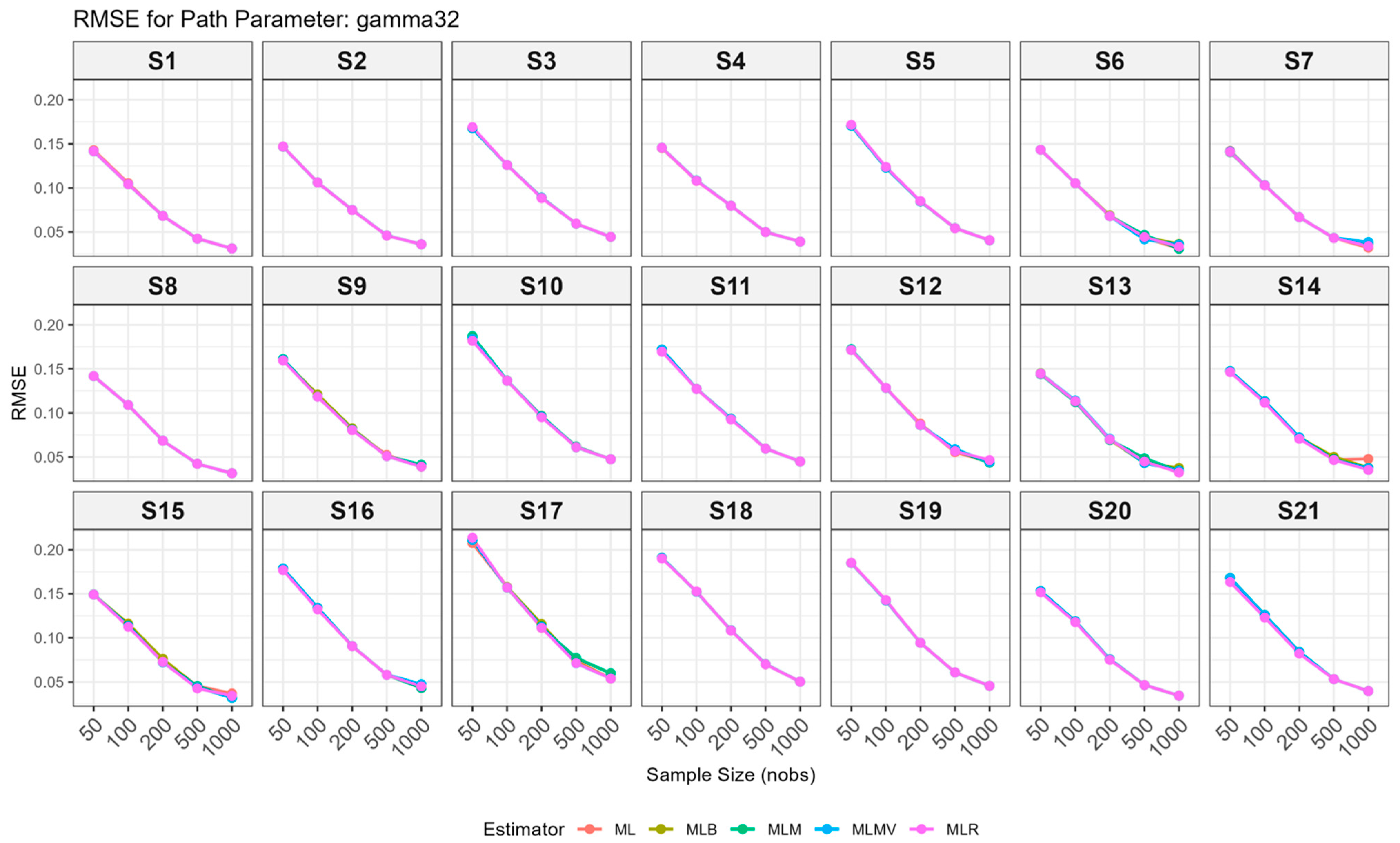
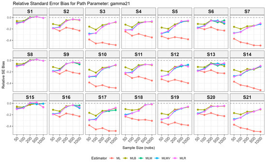
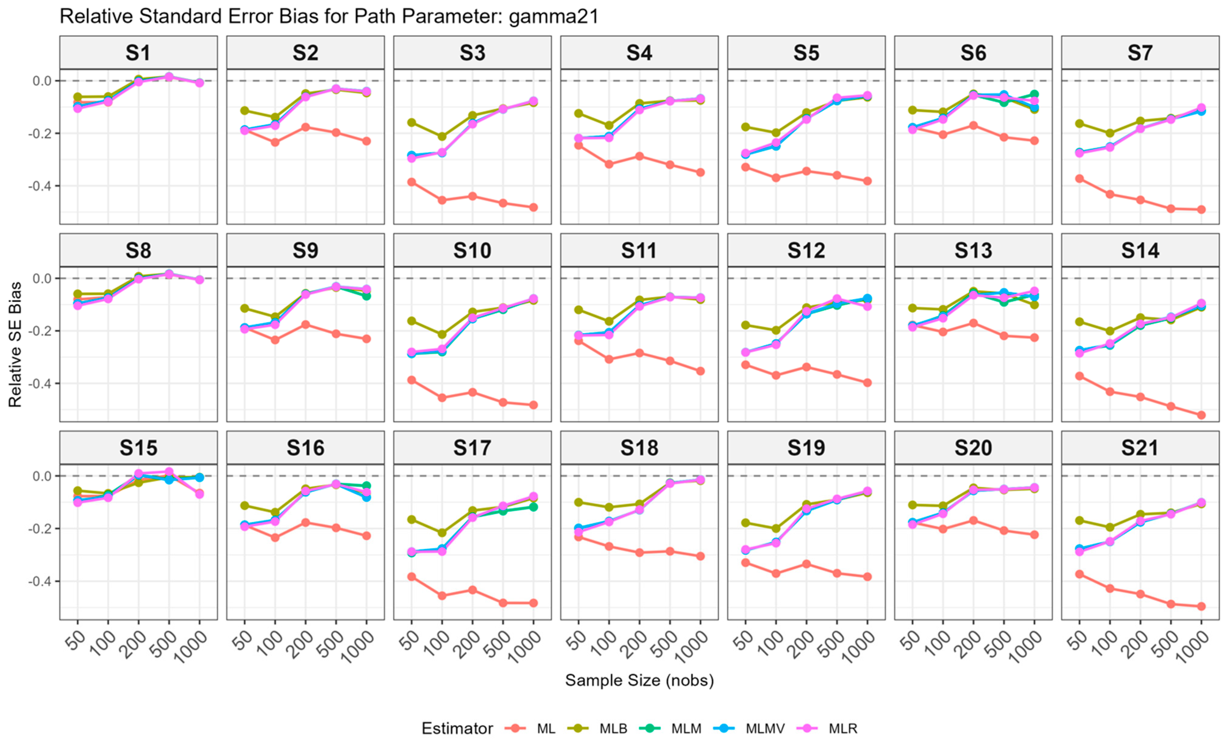
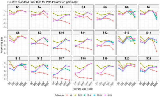
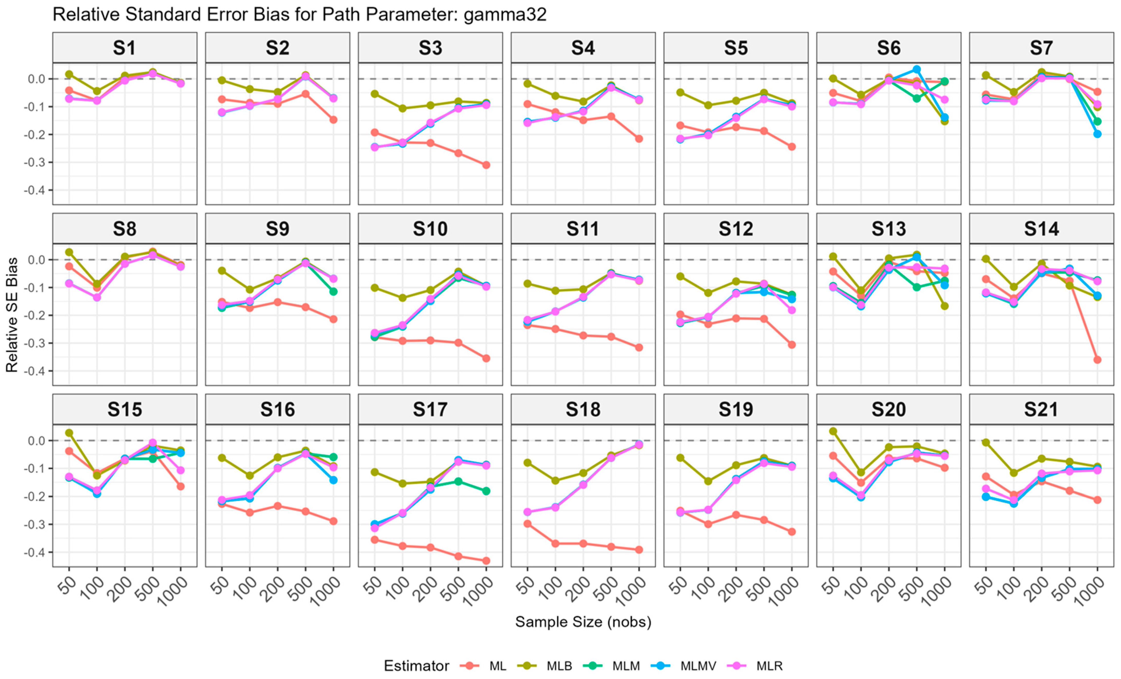
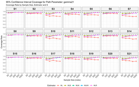
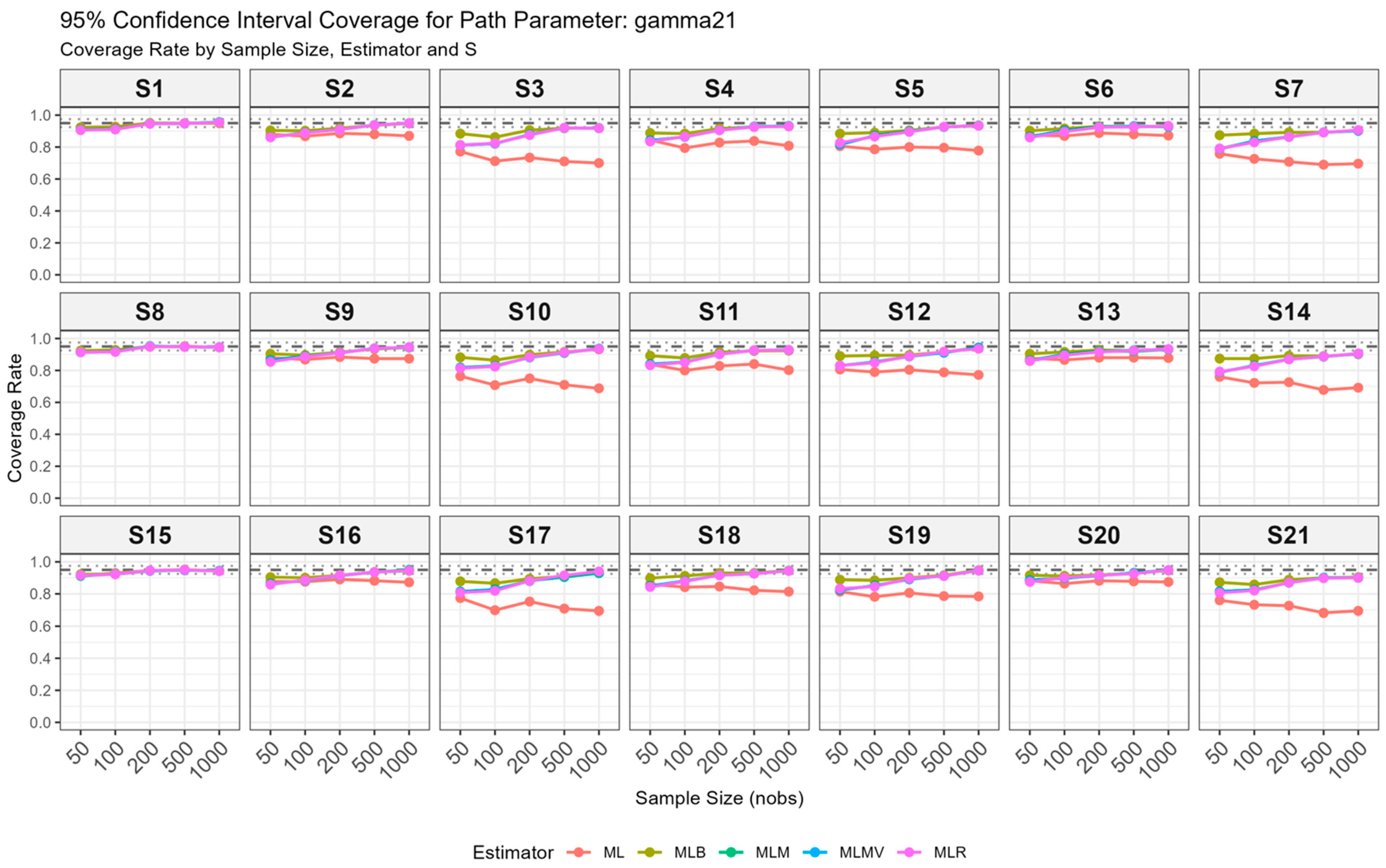
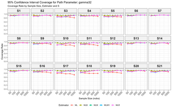
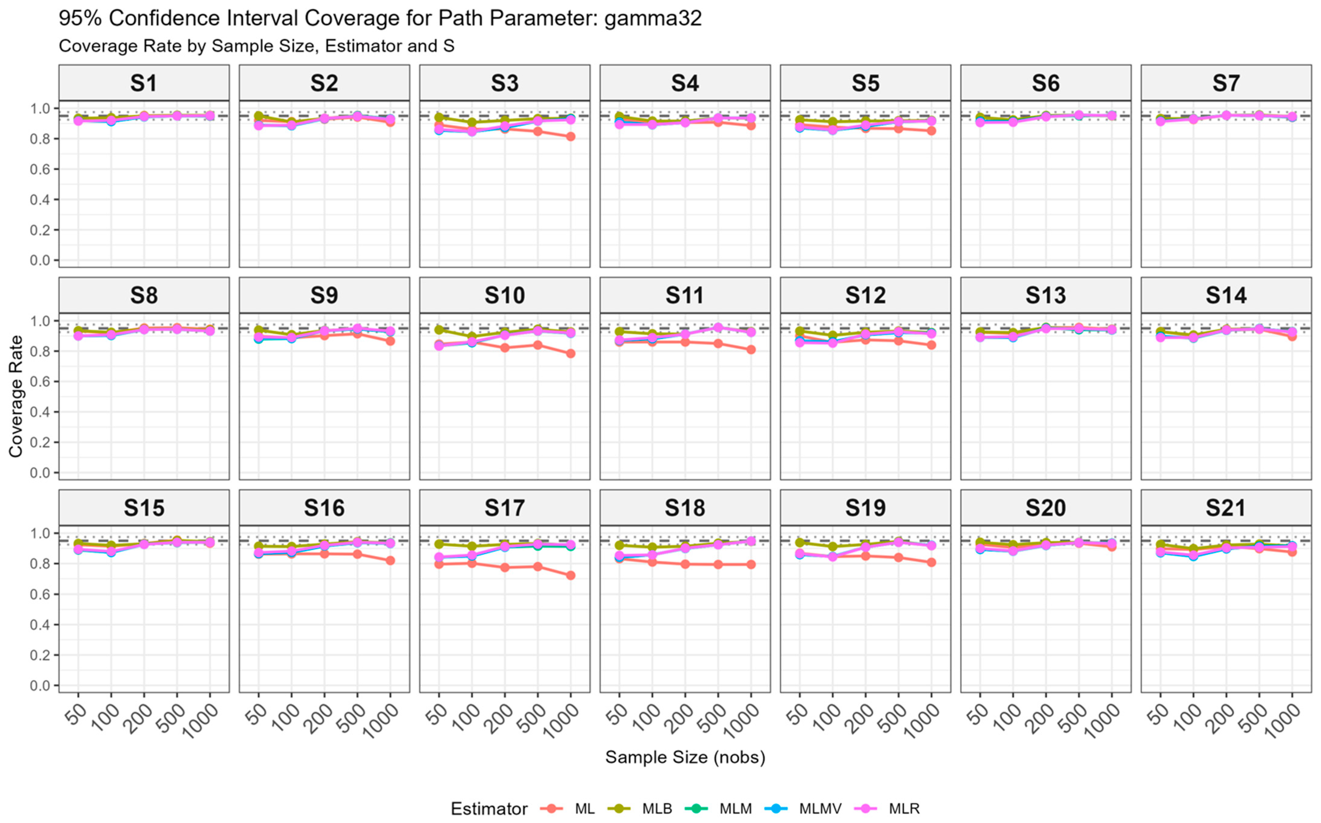
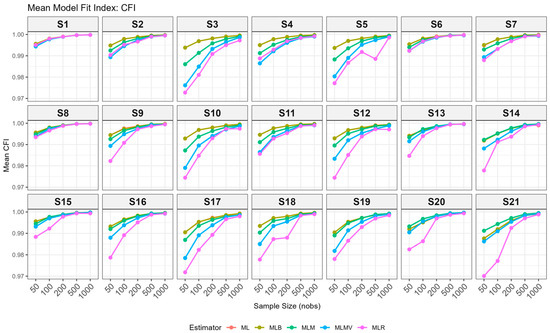
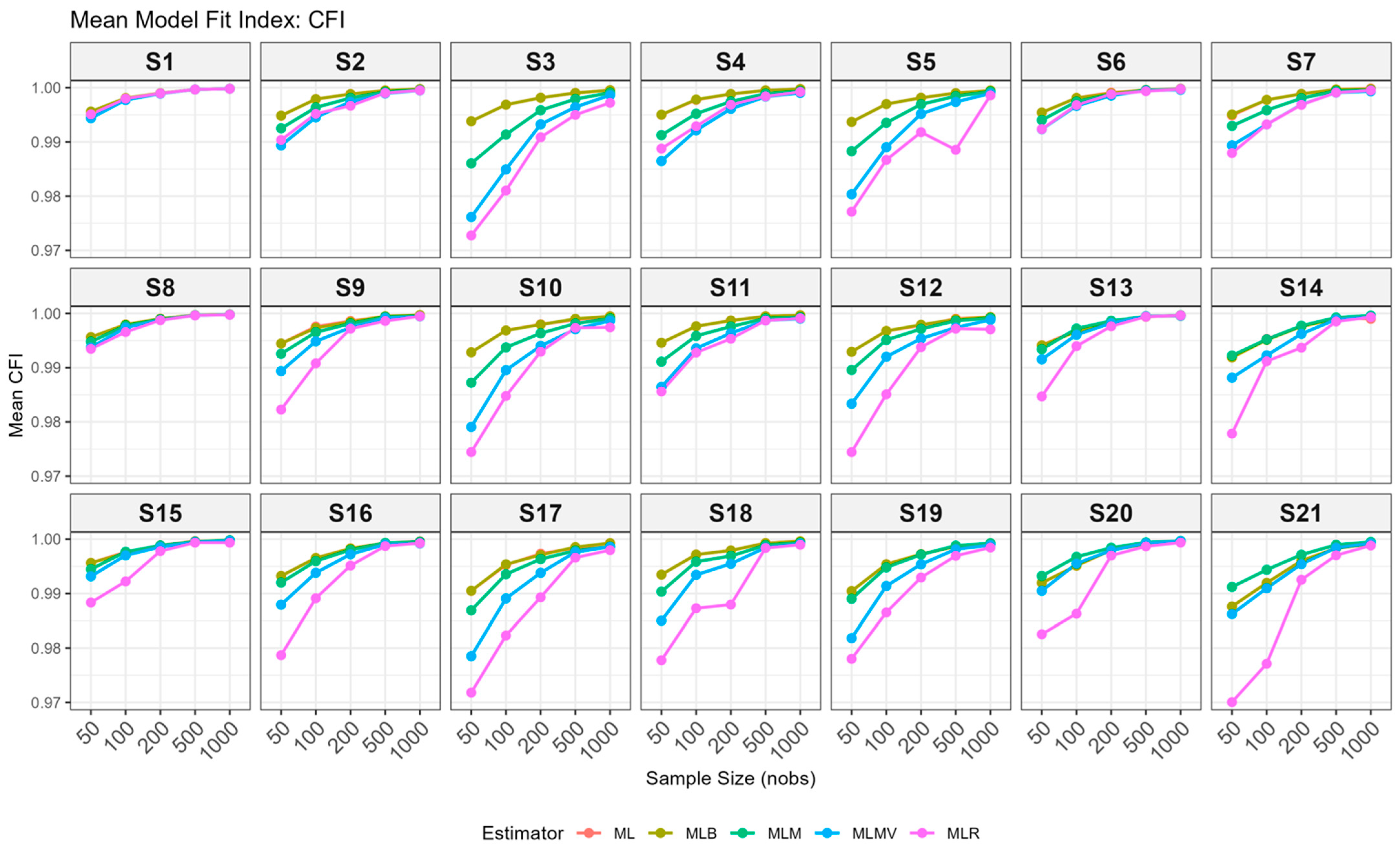
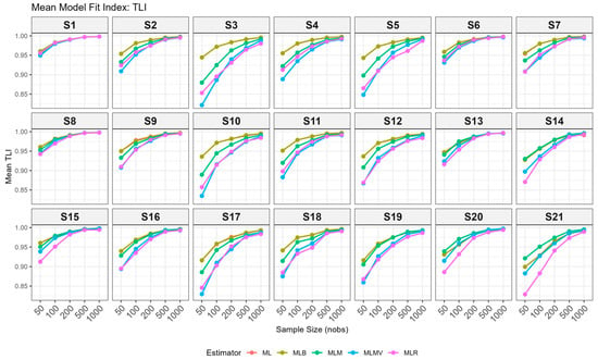
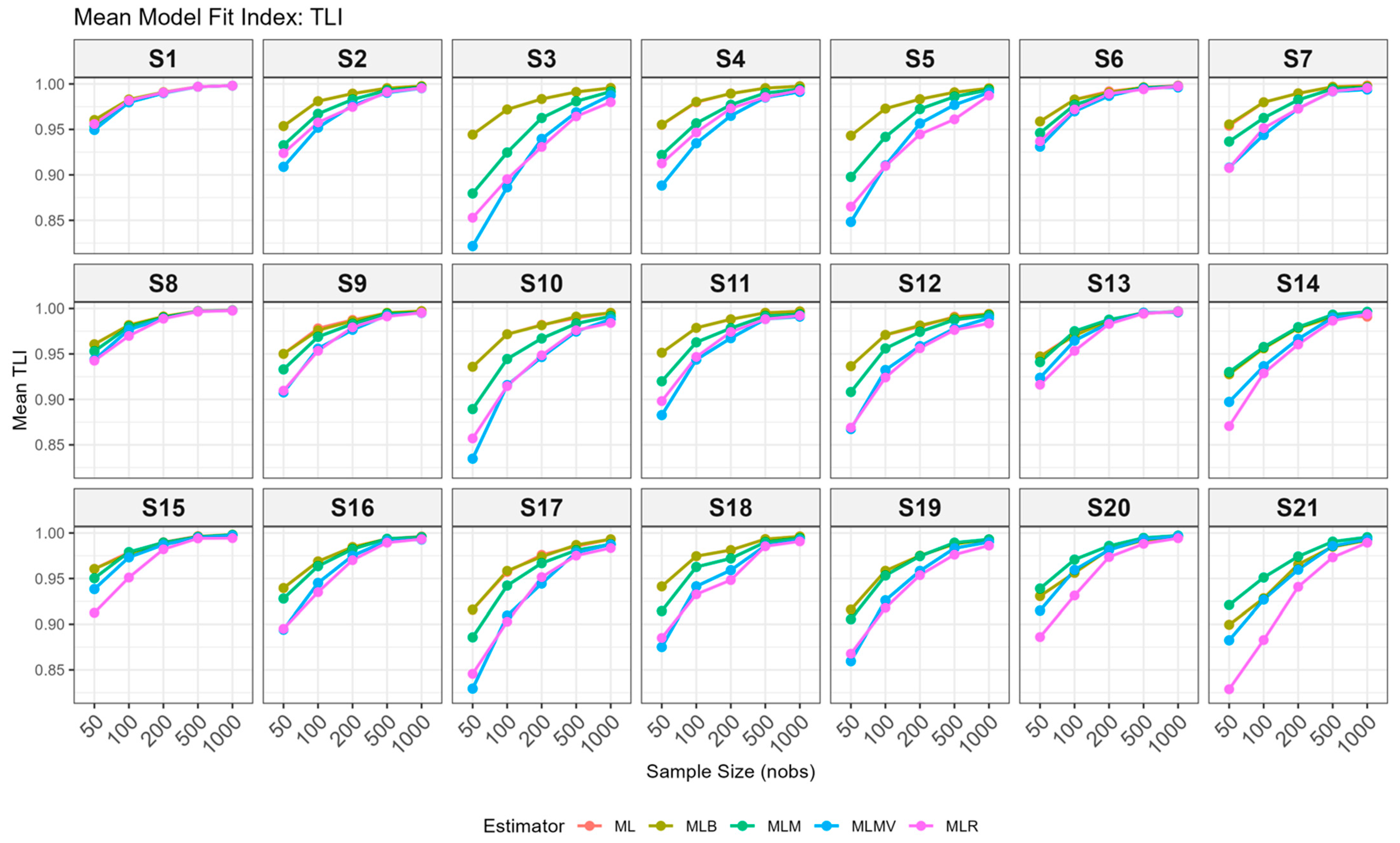
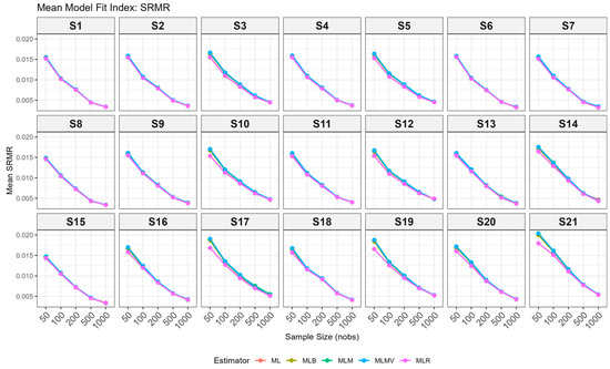
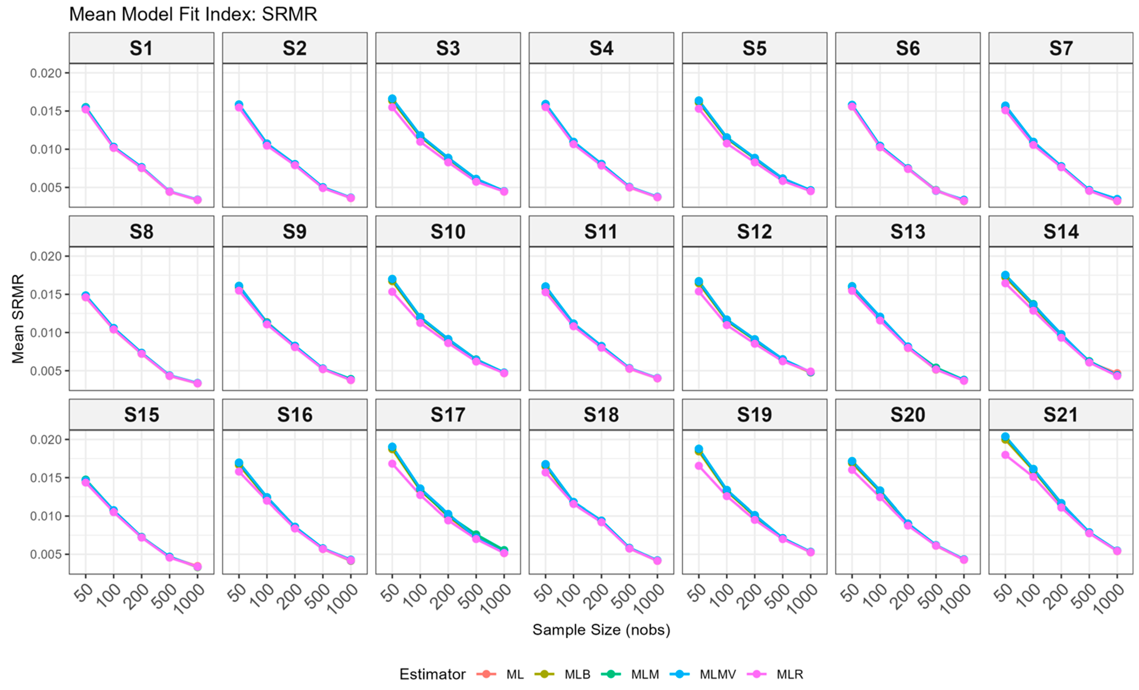
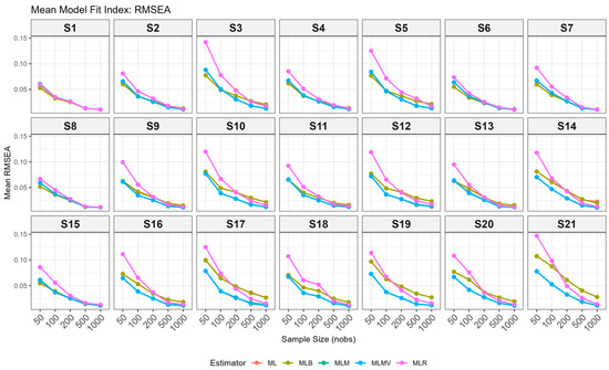
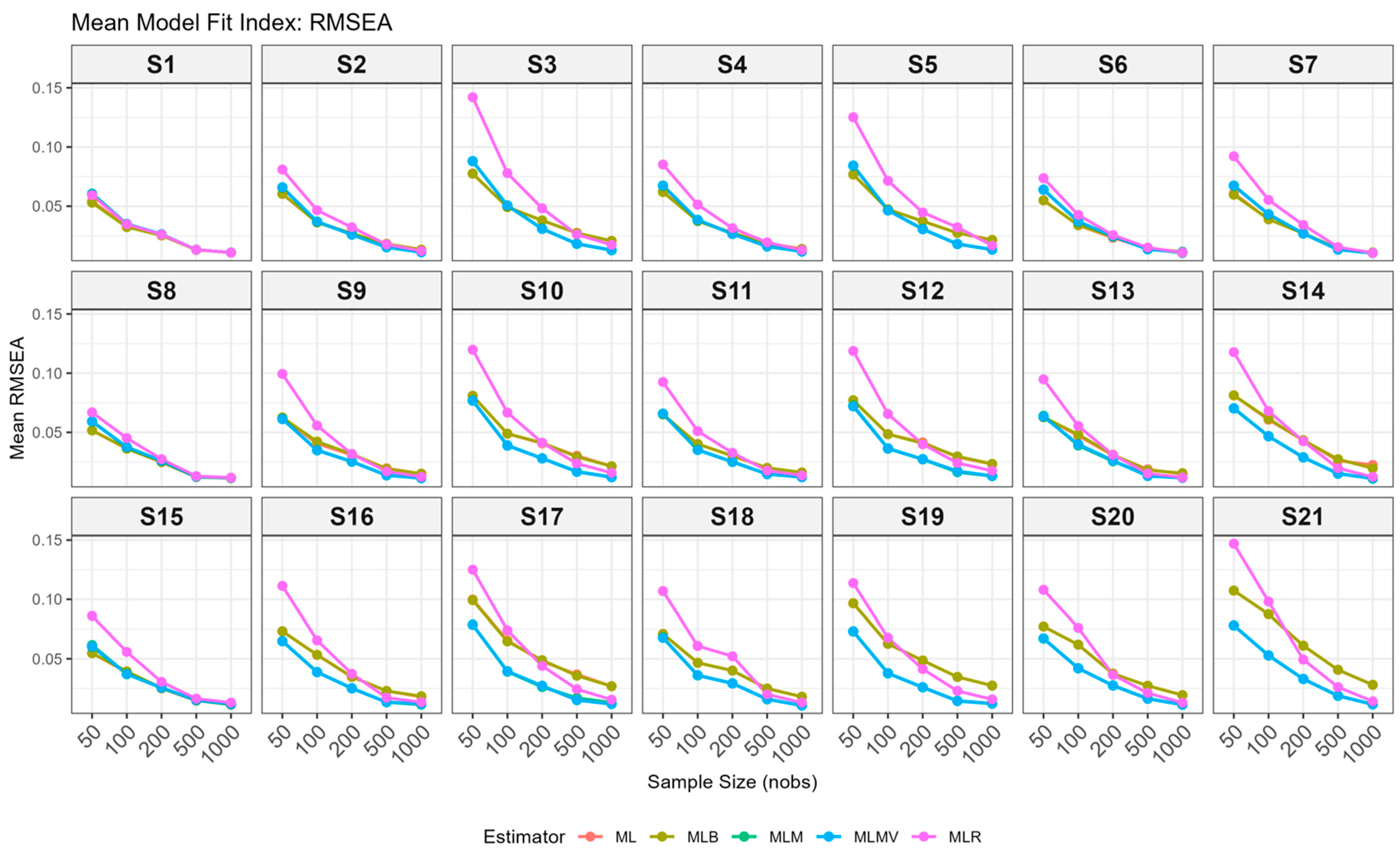
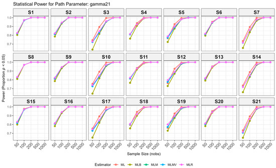
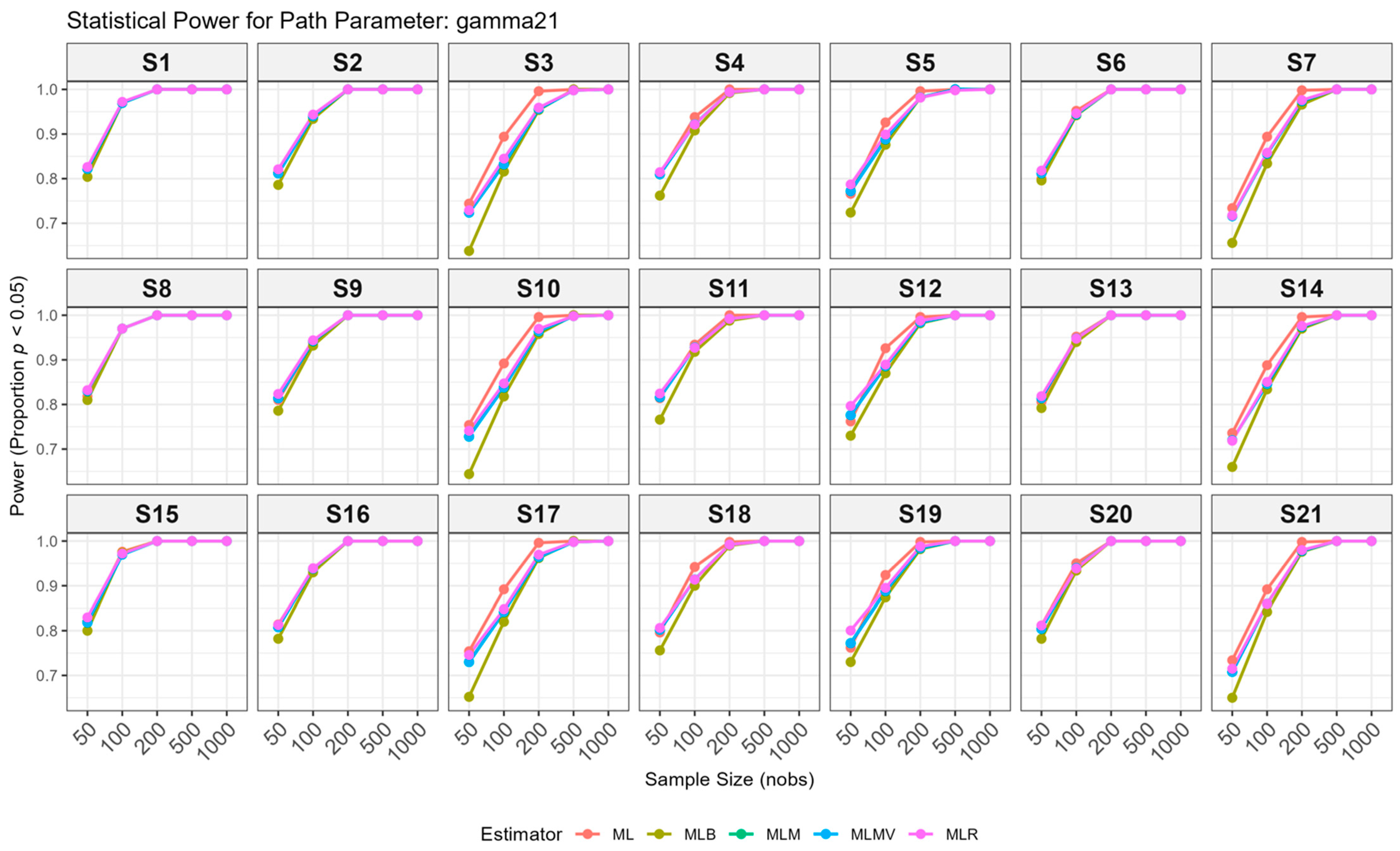
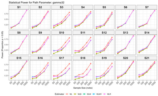
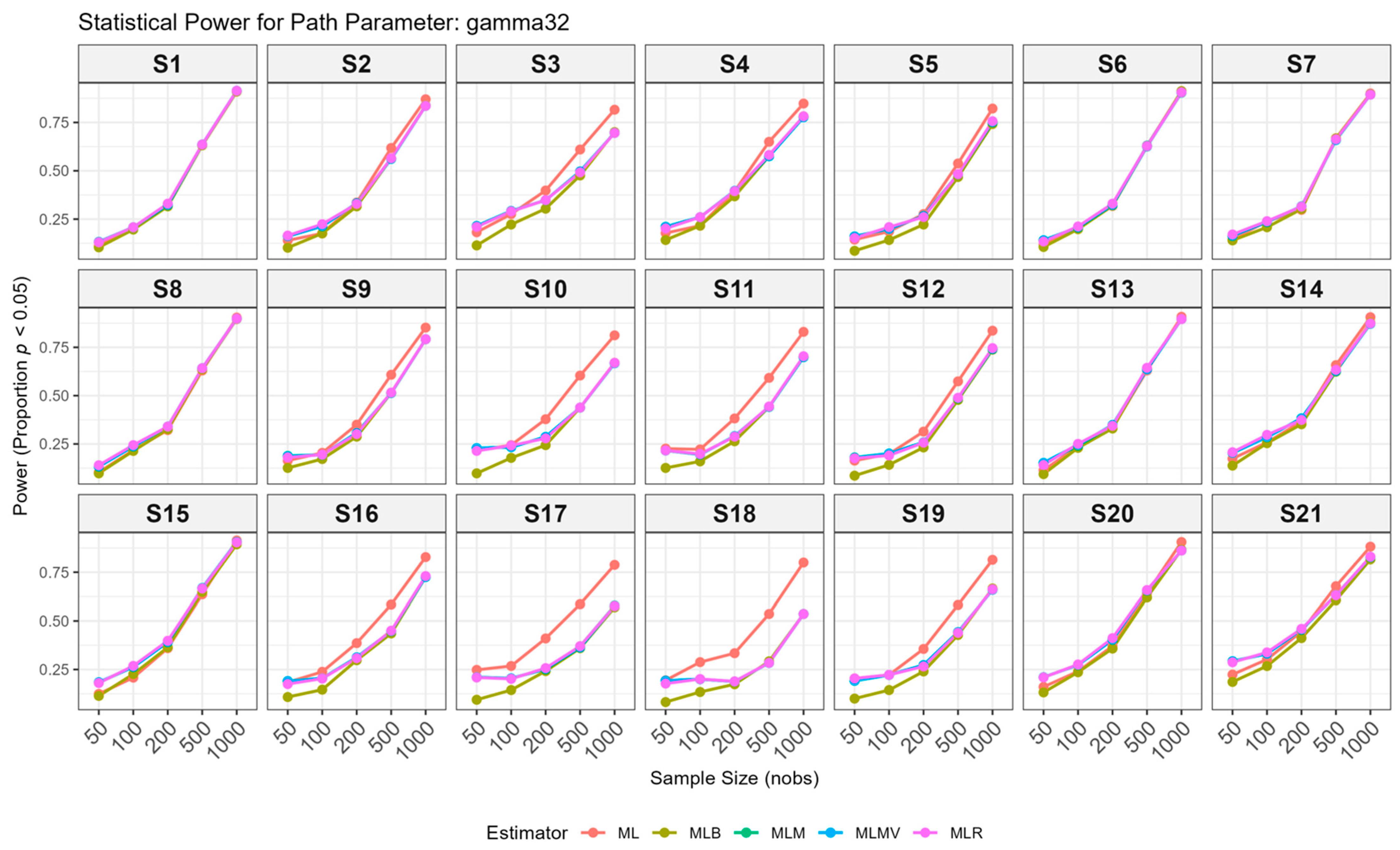

Disclaimer/Publisher’s Note: The statements, opinions and data contained in all publications are solely those of the individual author(s) and contributor(s) and not of MDPI and/or the editor(s). MDPI and/or the editor(s) disclaim responsibility for any injury to people or property resulting from any ideas, methods, instructions or products referred to in the content. |
© 2026 by the authors. Licensee MDPI, Basel, Switzerland. This article is an open access article distributed under the terms and conditions of the Creative Commons Attribution (CC BY) license.