


Abstract
Breast cancer remains a major global health concern, making accurate lesion assessment essential for effective clinical decision making. Deep learning has shown promising performance in breast ultrasound analysis, yet models evaluated on data from the same source may not generalize reliably to images acquired using different scanners and acquisition settings. This study therefore examines cross-dataset generalization and the factors that can improve it. Five lightweight YOLO instance-segmentation architectures (YOLOv8n, YOLO11n, YOLO11s, YOLO26n, and YOLO26s) were trained using a patient-grouped BUS-BRA protocol and a single training seed, and evaluated internally on held-out data and externally on BUS-UCLM, which served as the single target dataset. Ultrasound-specific preprocessing, test-time augmentation (TTA), and Optuna-selected configurations were assessed across 40 paired internal–external comparisons. Cross-dataset evaluation demonstrated consistent lesion delineation on BUS-UCLM, with matched Dice ranging from 0.861 to 0.875 and matched IoU from 0.764 to 0.786 across the five architectures. Preprocessing improved mask mAP@50–95 across all ten checkpoints on both datasets, while TTA improved detection-adjusted Dice despite having little effect on mAP@50–95. Optuna tuning improved external mAP@50–95 across all five architectures despite limited internal gains. Grad-CAM++ showed predominantly lesion-centered attention across both datasets, while ONNX Runtime deployment achieved 5.65–13.62 FPS on CPU. These findings highlight the importance of external validation, detection-aware evaluation, and efficient deployment for reliable breast ultrasound segmentation.
1. Introduction
Breast cancer requires timely and accurate lesion assessment to support appropriate clinical decision making. It remains the most frequently diagnosed malignancy among women worldwide, with approximately 2.3 million new cases and 665,684 deaths reported in 2022 [1]. In the United States, approximately 321,910 new cases of invasive female breast cancer and 42,140 associated deaths were projected for 2026 [2]. Moreover, the global burden of breast cancer is expected to increase, with approximately 3.2 million new cases and 1.1 million deaths projected annually by 2050. In many high-income countries, more than 80% of patients survive for at least five years after a breast cancer diagnosis, whereas survival remains considerably lower in settings where the disease is often detected at a later stage. As timely detection is important for improving survival, accessible and reliable diagnostic imaging plays a central role in supporting earlier diagnosis and better clinical outcomes [3].
Within this diagnostic pathway, breast ultrasound provides an accessible and practical imaging modality because it is portable, free of ionizing radiation, and particularly useful for evaluating dense breast tissue [4]. Consequently, it can serve as an important frontline modality in settings where mammographic screening programs are limited, while remaining a valuable adjunct elsewhere [5]. Nevertheless, ultrasound acquisition and interpretation depend on image quality, acquisition conditions, and clinical expertise, while variations in lesion appearance can complicate consistent assessment. In particular, speckle noise, low contrast, acoustic shadowing, and indistinct margins contribute to appreciable interobserver variability, thereby motivating the development of computational support tools [6,7].
Accordingly, deep learning has been extensively investigated for breast ultrasound analysis, with existing approaches broadly spanning three related tasks. Image-level classification has been addressed using transfer-learned convolutional backbones and architectures tailored to ultrasound texture [8,9,10,11,12], with further improvements explored through feature fusion and ensemble strategies [13,14,15]. Lesion delineation has primarily been investigated using encoder–decoder segmentation networks, sometimes coupled with a classification branch [16,17]. Meanwhile, detection-oriented single-stage models have been explored when localization and computational efficiency are jointly important, including applications in mammography and ultrasound [7,18,19,20,21,22]. Despite this progress, recent surveys emphasize that heterogeneous datasets, partitioning strategies, and evaluation metrics make performance difficult to compare reliably across studies [23,24,25].
More importantly, a persistent limitation concerns how breast ultrasound models are developed and evaluated. Many studies divide a single dataset into training and testing subsets and subsequently assess performance on images acquired from the same source. Although the test images are unseen during training, they generally share scanner characteristics, acquisition protocols, and low-level image statistics with the training data. Consequently, strong internal performance may reflect effective learning within a familiar imaging domain without necessarily demonstrating reliable generalization to a different clinical environment [23,25]. This concern becomes particularly important when a model trained on one dataset is evaluated on independently acquired data, where differences in scanners, institutions, transducers, gain, contrast, focus, resolution, post-processing, and speckle characteristics can substantially alter image appearance. Moreover, medical imaging models may exploit scanner- and site-related characteristics unrelated to the intended diagnostic target [26], while models that perform accurately within their development environment may degrade when acquisition conditions change. Consistent with this concern, cross-dataset analyses in breast ultrasound have reported performance degradation when the evaluation corpus changes [25].
To examine this problem directly, we incorporate ultrasound-specific preprocessing to normalize intensity and local contrast characteristics and apply the same preprocessing protocol during both internal and external inference. This controlled design allows us to determine whether improvements observed within the source domain persist after crossing the dataset boundary rather than assuming that internal gains transfer automatically. Specifically, BUS-BRA [27] serves as the source dataset with patient-level splitting, whereas BUS-UCLM [28] is reserved as an independent external dataset and contributes to no training, model selection, or adaptation decision.
Within this source-only cross-dataset framework, we benchmark five lightweight YOLO instance-segmentation architectures spanning three generations: YOLOv8n, YOLO11n, YOLO11s, YOLO26n, and YOLO26s [29,30,31,32]. In addition to preprocessing, Optuna-based hyperparameter optimization [33] is used to examine whether configurations selected exclusively through internal validation transfer effectively to external data. Test-time augmentation (TTA) is further evaluated to determine whether complementary inference views improve prediction robustness. Importantly, the evaluation separates lesion detection from delineation quality, allowing cross-dataset performance loss to be attributed more specifically to missed lesions, inaccurate boundaries, or both.
Beyond predictive generalization, practical deployment also requires consideration of computational efficiency and model interpretability. Breast ultrasound is particularly relevant in settings where dedicated computing infrastructure may be limited, motivating the evaluation of lightweight architectures that balance predictive performance with computational requirements [7,18,19,34,35]. Accordingly, we evaluate model size, computational cost, and inference latency and profile the trained models using ONNX Runtime on CPU. Furthermore, because quantitative performance alone provides limited insight into the spatial evidence underlying clinically sensitive predictions, Grad-CAM++ [36], a higher-order extension of gradient-weighted class activation mapping, is used to examine whether model attention remains concentrated on lesion-relevant regions across the internal and external datasets [8,9,10,14,37,38].
Taken together, this study moves beyond conventional within-dataset evaluation by jointly examining cross-dataset generalization, ultrasound-specific preprocessing, Optuna-based optimization, TTA, detection-aware segmentation performance, lightweight deployment, and explainability within a unified experimental framework. The specific contributions are as follows.
- Single-target cross-dataset evaluation: Five lightweight YOLO instance-segmentation architectures are trained exclusively on BUS-BRA under patient-level splitting and evaluated on both the held-out internal test fold and the independently acquired BUS-UCLM corpus, which contributes to no training, hyperparameter selection, or adaptation decision.
- Cross-dataset evaluation of methodological interventions: Ultrasound-specific preprocessing, test-time augmentation, and Optuna-based hyperparameter optimization are each evaluated on both corpora under an otherwise identical protocol, distinguishing interventions that improve internal performance from those whose benefits persist after a change in acquisition environment.
- Detection-aware cross-dataset analysis: Matched overlap and detection-adjusted overlap are reported separately, allowing cross-dataset performance differences to be attributed to missed lesions and changes in boundary delineation among successfully detected lesions.
- Operating-point and confidence analysis: Precision–recall behavior, confidence distributions of matched and missed lesions, and sensitivity across the decision-threshold range are examined to characterize threshold-dependent detection behavior and distinguish potentially recoverable sub-threshold predictions from lesions that remain undetected.
- Deployment efficiency and interpretability: Model size, computational cost, and CPU inference latency are profiled using ONNX Runtime, while Grad-CAM++ is applied to both datasets to examine whether model attention remains predominantly lesion-centered across internal and external evaluations.
Overall, by training exclusively on BUS-BRA and evaluating both within the source domain and without adaptation on BUS-UCLM, this study provides a controlled assessment of which strategies remain effective as acquisition conditions change, where performance is lost when generalization fails, and whether the resulting models remain computationally practical for deployment.
2. Related Work
Deep learning for breast ultrasound has developed most rapidly around lesion-level classification. A large body of work adapts general-purpose convolutional backbones to benign-versus-malignant classification, including VGG- and ResNet-derived designs [39,40], EfficientNet–ResNet hybrids with attention [41], Inception variants [11], and ensemble approaches [15,17]. Transformer and hybrid architectures have also emerged, including Swin-based multi-scale fusion networks [42] and vision transformers [43]. Comparative studies increasingly benchmark transfer-learned architectures across common breast ultrasound datasets [44,45,46,47]. To address limited annotated data, other studies have explored few-shot learning [48], generative augmentation [4,49], and optimized feature-selection strategies [13,50,51]. Broader developments are summarized in recent reviews [23].
Segmentation has developed alongside classification, particularly through encoder–decoder architectures. EfficientUNet variants and related U-shaped networks remain widely used for lesion delineation [16,52], while recent approaches incorporate richer contextual and refinement mechanisms [12,20]. Multimodal and clinically enriched frameworks have further combined imaging with additional information for diagnostic and outcome-related tasks [5,53,54,55,56].
The YOLO family provides an alternative when localization and computational efficiency are considered jointly. Successive generations have introduced changes to the backbone, neck, and detection head [29,30,57,58], with YOLO26 introducing an end-to-end NMS-free formulation and revised training strategy [31,32]. Comparative analyses describe the evolution of these architectures and their performance characteristics [59]. In breast imaging, YOLO-based approaches have been applied to mammography [18,60], automated breast volume scanning [7], and conventional ultrasound [19,21,61,62,63,64]. Recent pipelines have also combined detection with segmentation and automated hyperparameter optimization [22,65], while related evaluations in other medical applications demonstrate the efficiency potential of compact YOLO variants [34,35].
Explainability and systematic optimization have increasingly accompanied predictive modeling. Grad-CAM and Grad-CAM++ are widely used to visualize image regions contributing to model predictions, including in breast ultrasound applications [8,9,10,14,37,38]. Automated hyperparameter optimization has likewise been adopted to configure deep learning pipelines more systematically than manual search [6,24].
The availability of BUS-BRA [27] and BUS-UCLM [28] has made evaluation across independently acquired breast ultrasound datasets increasingly feasible, while comparative studies have begun to report performance across multiple sources [25]. Nevertheless, three gaps remain: cross-dataset validation of breast ultrasound segmentation is limited; the transferability of preprocessing, hyperparameter optimization, and TTA across independent datasets remains insufficiently studied; and aggregate segmentation metrics provide limited insight into whether performance degradation arises from lesion detection or delineation. Accordingly, this study examines these issues within a unified source-only cross-dataset framework, complemented by explainability and CPU deployment analysis.
3. Materials and Methods
3.1. Study Design
This study follows a source-only cross-dataset design, with BUS-BRA used for model development and BUS-UCLM reserved exclusively for external evaluation. Figure 1 summarizes the complete framework, including preprocessing, Optuna optimization, TTA, Grad-CAM++, and ONNX Runtime deployment.
Figure 1.
Overview of the source-only cross-dataset breast ultrasound segmentation study. The outer labels summarize the BUS-BRA source corpus with patient-grouped leakage control, the BUS-UCLM external evaluation corpus, five YOLO architectures, two training arms, preprocessing and TTA conditions, Grad-CAM++ analysis, and ONNX Runtime CPU profiling.
3.2. Datasets
Two independently acquired, publicly available breast-ultrasound corpora with pixel-level lesion annotations and pathology labels are used. BUS-BRA [27] serves as the source domain and BUS-UCLM [28] as the external target domain. The two share an identical label space, benign and malignant, allowing direct comparison of internal and external metrics without label remapping. BUS-UCLM comprises 683 frames in total, of which the 264 lesion-bearing frames with pixel-level lesion annotations were used for external evaluation; the remaining 419 lesion-free frames were excluded. Consequently, false-positive behavior on normal tissue is not assessed, and the reported external metrics characterize detection and delineation on lesion-bearing frames only. Table 1 summarizes the evaluated images and lesion counts for both corpora, and Figure 2 shows representative frames with their ground-truth masks.
Table 1.
Evaluated image composition and lesion counts for internal and external evaluation.
Figure 2.
Representative BUS-BRA and BUS-UCLM images with ground-truth lesion masks, illustrating cross-dataset differences in ultrasound appearance.
The near-identical class priors shown in Figure 3 are important for interpretation: because the benign fraction differs by less than two percentage points between corpora, the observed external performance differences are unlikely to be driven primarily by a shift in the marginal class distribution.
Figure 3.
Class distribution of BUS-BRA and BUS-UCLM, showing comparable benign-to-malignant ratios across datasets.
3.3. Annotation Conversion
Both corpora distribute lesion annotations as masks, which are converted to YOLO polygon format. BUS-BRA masks are binary, so the class label is taken from the accompanying metadata. BUS-UCLM masks are color-coded, with green denoting benign and red denoting malignant lesions, so each color channel is decoded into its own instance; grayscale masks fall back to the metadata label. Contours are extracted with external retrieval, and those covering less than 0.05% of the frame area are discarded as annotation speckle. Retained contours are simplified using a polygonal curve simplification procedure with a tolerance of 0.2% of the contour perimeter and are subsequently normalized to image coordinates. Images yielding no valid polygon are dropped from the corresponding split.
3.4. Patient-Grouped Splitting and Leakage Control
BUS-BRA is partitioned with StratifiedGroupKFold using ten folds, grouping by patient identifier and stratifying by pathology. The first fold becomes the test set, the second the validation set, and the remaining eight the training set, producing an exact 80/10/10 partition in which no patient appears in more than one split while the benign-to-malignant ratio is preserved across splits. Because breast-ultrasound corpora frequently contain multiple frames or bilateral views per patient, random image-level splitting would place correlated frames of the same lesion on both sides of the train–test boundary and inflate internal performance. The absence of such leakage is enforced programmatically rather than assumed: the pipeline asserts that every patient identifier maps to exactly one split and fails otherwise.
3.5. Ultrasound-Specific Preprocessing
For model development, BUS-BRA training and validation images are processed using the ultrasound-specific preprocessing chain described below. During evaluation, each frozen checkpoint is tested under two input conditions: the original raw image and the corresponding preprocessed image. This paired design allows the effect of inference-time preprocessing to be evaluated on fixed model weights across both the held-out BUS-BRA test set and the independent BUS-UCLM dataset.
For the preprocessed condition, images are read as single-channel grayscale, intensity-clipped to the 1st and 99th percentiles and rescaled to the full 8-bit range, then enhanced with contrast-limited adaptive histogram equalization (CLAHE) [66] using a clip limit of 2.0 and an tile grid, and finally replicated to three channels for network input. Percentile clipping suppresses extreme intensity values associated with calipers, annotation overlays, and transducer artifacts, while CLAHE reduces variation in local contrast across ultrasound images.
Order of operations and execution: The preprocessing chain is applied in a fixed order: (i) conversion to single-channel grayscale; (ii) intensity rescaling by clipping at the 1st and 99th percentiles of that image and linearly mapping the retained range to ; (iii) contrast-limited adaptive histogram equalization on an tile grid with clip limit ; and (iv) replication of the enhanced single channel across three channels, after which the framework applies aspect-ratio-preserving letterboxing to 640 pixels. The chain contains no fitted parameters and no cross-image statistics, so applying it to the validation fold, the internal test fold, and BUS-UCLM introduces no information leakage. It is executed on the fly at inference time on every evaluated frame, which is why its cost appears in the end-to-end latency reported in Section 4.10; during training, the same chain is applied when the datasets are materialized.
3.6. Offline Scanner Simulation
Only the BUS-BRA training split additionally receives offline scanner-oriented copies, one per training image, generated after preprocessing. Scanner simulation is used strictly as a training-stage data-augmentation method. It is applied only to the BUS-BRA training split and never to the validation fold, the internal test fold, or any BUS-UCLM frame, and it is therefore not an evaluation condition anywhere in this study. These transformations perturb intensity and texture statistics while leaving lesion geometry untouched, so the polygon labels of a scanner-augmented copy are identical to those of its source image. The components and their sampling ranges are given in Table 2. Gamma, contrast, gain, and brightness are applied to every copy; a Gaussian electronic-noise term and a multiplicative speckle term are mutually exclusive alternatives drawn with equal probability; focus is left unchanged, blurred, or sharpened; and effective resolution is occasionally reduced and restored. Because the augmented copies are materialized once with a deterministic per-image seed rather than sampled afresh each epoch, the training corpus is exactly reproducible.
Table 2.
Scanner-simulation components applied to the BUS-BRA training split.
In addition, conservative online geometric augmentation is enabled during training: rotation up to , translation up to 5%, scaling up to 15%, shear up to , horizontal flipping with probability 0.5, and value-channel jitter of 0.15. Mosaic, mixup, cutmix, copy-paste, and random erasing are disabled, because compositing multiple ultrasound frames or occluding regions produces images with no physical counterpart in a real examination and can move lesion boundaries into implausible contexts.
3.7. Architectures and Their Differences
Five instance-segmentation architectures are benchmarked, spanning three generations of the YOLO family and two capacity tiers within the newer two. YOLOv8n [29] provides the established baseline; YOLO11n and YOLO11s [30] adopt the revised backbone and neck of the eleventh generation; and YOLO26n and YOLO26s [31,32] adopt the end-to-end, NMS-free detection head. Because the three generations differ in ways that bear directly on the questions this study asks, namely cross-dataset robustness and CPU-side deployability, their design is described in turn before the results are presented. Table 3 summarizes the generational differences, and Table 4 gives the resulting cost profile of the five specific checkpoints.
Table 3.
Architectural differences among the YOLO families evaluated in this study. The asterisk (*) denotes deployment-related changes introduced in YOLO26.
Table 4.
Architectural and computational characteristics of the five benchmarked YOLO segmentation models.
3.7.1. Shared Skeleton and Segmentation Head
All five models retain the three-stage backbone–neck–head skeleton common to the Ultralytics lineage [59]. The backbone extracts features at strides 8, 16, and 32 using cross-stage partial blocks and terminates in a fast spatial pyramid pooling (SPPF) stage that widens the receptive field cheaply. The neck fuses these three scales through a top-down feature-pyramid path followed by a bottom-up path-aggregation path, which matters for breast ultrasound because lesion diameter varies widely within a single corpus and the smaller lesions survive only if fine-stride features reach the head intact. The head is decoupled and anchor-free in every generation considered here, so no anchor priors tuned to a particular scanner’s field-of-view conventions are carried across the domain boundary.
Instance segmentation is realized by a prototype-and-coefficient formulation rather than by a per-region mask branch. A prototype module emits 32 mask bases at resolution for the whole image, and each detection predicts 32 coefficients whose linear combination with those bases, cropped to the detected box, yields the instance mask. This is visible directly in the exported graphs of Table 4: every model carries a prototype output, and the 38 channels of the detection output decompose as four box parameters, two class scores, and 32 mask coefficients for YOLOv8 and YOLO11. The practical consequence is that mask cost is almost independent of the number of lesions present, and that detection and delineation are only loosely coupled: the prototype basis can describe a lesion accurately even when the detection branch scores it below threshold. This architectural separation is what makes the matched-versus-detection-adjusted decomposition of Section 3.12 meaningful rather than merely arithmetic.
3.7.2. YOLOv8: Anchor-Free Baseline
YOLOv8 established the configuration the later generations refine. Its backbone and neck are built from C2f blocks, cross-stage partial units that split the input, pass one branch through a series of bottlenecks, and concatenate every intermediate output, which enriches gradient flow at moderate parameter cost [29]. Its head is anchor-free and decoupled, with separate classification and regression branches, and box coordinates are predicted through distribution focal loss (DFL), a distributional formulation in which each coordinate is regressed as a discrete probability distribution over candidate positions rather than a single scalar. Label assignment is one-to-many, so a ground-truth lesion is matched to several positive locations during training and the resulting duplicate predictions must be removed at inference by non-maximum suppression (NMS).
3.7.3. YOLO11: Cheaper Blocks and Selective Attention
YOLO11 keeps the anchor-free, DFL-based head of YOLOv8 and changes the feature extractor in two respects [30,59]. First, the C2f block is replaced by C3k2, a cross-stage partial bottleneck built from smaller kernels, which lowers the operation count for a given depth. Second, a C2PSA block combining cross-stage partial structure with position-sensitive self-attention is inserted immediately after SPPF, at the lowest spatial resolution, where attention is affordable. The classification branch also moves to lighter depthwise-separable convolutions. The net effect at nano scale is a model that is smaller and cheaper than its predecessor while remaining competitive, which Table 4 confirms for the checkpoints trained here: YOLO11n uses M parameters and GFLOPs against M and GFLOPs for YOLOv8n. The added attention stage is motivated by exactly the conditions that characterize ultrasound, low contrast against a cluttered background and partially obscured object boundaries, since it lets the network weight informative regions before the neck fuses scales.
3.7.4. YOLO26: End-to-End, DFL-Free and Deployment-Oriented
YOLO26 retains the C3k2 and C2PSA feature extractor but restructures the head and the training recipe around deployment [31,32]. Four changes matter here. The distributional box regression of the previous two generations is removed in favor of direct coordinate regression, simplifying the regression pathway for deployment. Label assignment becomes one-to-one, so the network learns to emit a single prediction per object and NMS is eliminated; inference therefore becomes a direct mapping from the input image to a fixed-size set of final detections. Progressive loss balancing (ProgLoss) adjusts the relative weighting of loss terms over the course of training instead of holding it fixed, and small-target-aware label assignment (STAL) preferentially assigns labels to small or partially occluded objects. Finally, the recipe introduces MuSGD, a hybrid optimizer blending stochastic gradient descent with Muon-style curvature and momentum behavior.
These architectural differences are also reflected in the exported model structure. The NMS-free head enables YOLO26 to emit the fixed tensor shown in Table 4, in which the 38 channels represent four box parameters, a confidence value, a class index, and 32 mask coefficients. YOLO26n also records the largest ONNX Runtime speed-up in the study at (Section 4.10). Its NMS-free formulation may contribute to this deployment advantage by removing the need for a separate suppression stage; however, the present profiling does not isolate the contribution of the NMS-free head from other architectural and runtime differences. MuSGD provides a separate observation from the hyperparameter search: although it was offered to every architecture on equal terms, the Optuna study selected the MuSGD trial for three of the five models, YOLO11s, YOLO26n, and YOLO26s, and the AdamW trial for the two older-generation nano models (Section 3.9).
3.7.5. Rationale for a Single-Stage Instance-Segmentation Family
The choice of this model family follows from the structure of the clinical task rather than from an assumption that it outperforms all alternatives. A breast-ultrasound analysis system must determine whether a lesion is present, delineate its boundary, and assign a lesion class. Instance segmentation addresses these tasks within a unified framework and provides per-lesion predictions, whereas semantic segmentation methods such as U-shaped encoder–decoder networks [12,16,52] primarily produce pixel-level segmentation maps. Two-stage instance-segmentation approaches can also provide lesion-level outputs but introduce an additional proposal stage, making single-stage architectures attractive when computational efficiency is an important design constraint.
Three further properties motivated the choice of this family. First, its prototype-based mask formulation enables lesion detection and segmentation within the same inference pipeline. Second, the YOLO family provides established export paths to ONNX Runtime, allowing deployment efficiency to be evaluated directly; the resulting CPU performance is reported in Section 4.10. Third, per-lesion predictions enable the one-to-one matching required by the detection-adjusted overlap metrics used to distinguish missed lesions from poor delineation. Previous studies in breast and other organ imaging have also reported competitive performance of YOLO-family models while retaining relatively low inference cost [7,18,19,25,34,35], further supporting their evaluation in the present setting.
This study did not perform head-to-head comparisons with U-Net variants, Mask R-CNN, or transformer-based segmentation models. The selection of the YOLO family should therefore be interpreted as a design choice motivated by lesion-level prediction, deployment requirements, and prior literature rather than as evidence of superiority over other segmentation families. The experiments instead establish the relative behavior of five lightweight YOLO architectures under cross-dataset shift. As shown in Section 4.6, their internal ranking does not reliably predict their external ranking, further emphasizing the importance of external evaluation when comparing models for breast-ultrasound applications.
3.8. Training Configuration
All architectures are trained with an identical fixed configuration, listed in Table 5, so that any performance difference is attributable to architecture or to the searched hyperparameters rather than to the training budget. Only the optimizer, initial learning rate, final learning-rate factor, and weight decay are allowed to vary, and only through the Optuna study described below. All experiments were run with the Ultralytics package version 8.4.90 on PyTorch 2.13, with Optuna 4.9.0 used for the hyperparameter search and ONNX Runtime 1.27.0 used for the deployment profiling. All four packages were accessed on 8 July 2026.
Table 5.
Fixed training configuration, identical for all five architectures and all five trials.
3.9. Hyperparameter Optimization
Each architecture receives one independent Optuna study [33] driven by a tree-structured Parzen estimator sampler, maximizing mask mAP@50–95 measured on the BUS-BRA validation split only. The search space covers the optimizer (AdamW, SGD, or MuSGD), the initial learning rate ( to , log-uniform), the final learning-rate factor (0.05 to 0.5, log-uniform), and weight decay ( to , log-uniform). Five trials are run per architecture. Trials 0–2 are seeded to explore one optimizer each, Trial 3 is unconstrained, and Trial 4 is enqueued with the fixed parameter values listed in Table 6 and serves as the comparison configuration for evaluating the selected tuned trials. The tuned checkpoint for each architecture is the best-scoring trial among Trials 0–3, selected on validation performance alone. Table 6 lists the complete trial configurations and resulting selections.
Table 6.
Optuna trial configurations and selected trials for each YOLO architecture.
The five-trial budget was determined by the available computational resources. All training was performed on the Kaggle platform using dual NVIDIA T4 accelerators, with accelerator access limited to approximately 30 h per week and individual sessions limited to 12 h. Extending the search to 20–30 trials across all five architectures would have exceeded the available allocation.
No BUS-UCLM image influenced hyperparameter selection. Accordingly, the external improvements reported in Section 4.5 represent positive transfer of configurations selected on the source dataset rather than optimization of external performance.
3.10. Test-Time Augmentation
Test-time augmentation is applied post hoc to frozen checkpoints and therefore changes no learned parameter. Each image is passed through the network twice, once unaltered and once horizontally mirrored, with predictions from the mirrored view mapped back to the original coordinate frame. Candidate instances are sorted by confidence and fused greedily: a candidate joins an existing group when it shares the group’s class and overlaps it with mask IoU at least , and each group’s final mask is the confidence-weighted vote of its members thresholded at , with the bounding box formed by the corresponding weighted mean. Vertical flipping is deliberately excluded, since breast-ultrasound frames have a fixed skin-to-depth orientation and vertical mirroring produces anatomically impossible images.
3.11. Statistical Treatment of Paired Comparisons
Every configuration was trained once, under a fixed seed with deterministic execution enabled, so run-to-run variance attributable to random initialization and data ordering was not estimated. Paired comparisons are therefore controlled by design rather than by repetition: each intervention is evaluated by toggling one factor while architecture, tuning arm, dataset and all remaining factors are held fixed, which yields 20 matched pairs per comparison per dataset. Reported effect magnitudes and win counts describe those matched pairs, and small per-architecture differences should not be over-interpreted.
To quantify the uncertainty that is estimable from this design, each paired comparison is additionally summarized by a bias-corrected percentile bootstrap 95% confidence interval over the 20 matched differences (10,000 resamples, seed 42) and by a two-sided Wilcoxon signed-rank test on the same differences. These statistics characterize the consistency of an intervention across architectures, tuning arms and inference conditions; they do not substitute for seed-level variance, and no claim of significance is made for architecture-to-architecture differences, which remain single-run observations. Results appear in Section 4.3.
3.12. Evaluation Metrics
Metric nomenclature: All average-precision values reported in this manuscript are computed on mask predictions rather than on bounding boxes. Two are used throughout: mAP@50, the mean average precision at a single mask intersection-over-union threshold of , and mAP@50–95, the mean average precision over ten mask IoU thresholds from to in steps of . For brevity, the qualifier “mask” is omitted after this definition. Overlap statistics are abbreviated as mDice and mIoU for mean matched Dice and IoU over successfully detected lesions, and as aDice and aIoU for their detection-adjusted counterparts, in which every undetected ground-truth lesion contributes zero. P, R, and denote the macro-averaged class-specific precision, recall, and score, respectively. For each class, is the harmonic mean of class-specific precision and recall. The class-specific values are obtained from the precision–recall curve at mask IoU at the maximum- operating point, selected independently for each class, architecture, corpus, and condition. The overlap statistics mDice, mIoU, aDice, and aIoU are computed at the fixed reference confidence threshold of .
All reported results use a single custom segmentation-metric backend so that conditions with and without test-time augmentation are evaluated identically. For class c, with true positives (), false positives (), and false negatives (), precision, recall, and are defined as
When a denominator is zero, the corresponding class-specific value is defined as zero. The reported P, R, and values are the arithmetic means of , , and , respectively, over the two classes.
For class c and mask-IoU threshold , average precision is computed over 101 recall points as
where denotes the maximum precision obtained at any recall level . The two reported mean average-precision measures are
and
where corresponds to the benign and malignant classes.
At the fixed reference confidence threshold of , predictions are matched one-to-one to ground-truth lesions of the same class using greedy mask IoU with a minimum matching threshold of . For a predicted mask and its matched ground-truth mask , Dice and IoU are defined as
Let denote the number of successfully matched ground-truth lesions. The mean matched overlap measures are
These measures quantify delineation quality conditional on successful lesion detection. All evaluated conditions contained at least one successfully matched lesion, so throughout the reported analyses.
Let denote the total number of ground-truth lesions. The detection-adjusted measures are
Thus, every unmatched ground-truth lesion contributes zero. Reporting both matched and detection-adjusted overlap separates delineation quality from lesion-detection failure: stable matched overlap together with lower detection-adjusted overlap indicates that successfully detected lesions remain well delineated while a greater proportion of lesions are missed.
Grad-CAM++ maps were generated post hoc from the trained YOLO26s-seg checkpoint for representative benign and malignant cases from the BUS-BRA test set and BUS-UCLM. The same model weights and visualization procedure were used for both datasets to permit direct comparison of attention patterns.
Operating Threshold
The reported metrics follow three distinct operating conventions, and the distinction matters for how each should be interpreted. All are computed from the same set of predictions, which is generated with a confidence floor of so that the full operating range is available to the evaluator.
Threshold-free metrics: Mask mAP@50 and mAP@50–95 integrate the precision–recall curve over the entire confidence range and are therefore invariant to any choice of operating point.
Summary precision, recall, and : These are read from the precision–recall curve at mask IoU at its maximum- point, selected independently for each class, architecture, corpus, and condition and then macro-averaged over the two classes. They therefore describe the best balance of precision and recall that each configuration can attain rather than performance at any one fixed confidence value, and they are the values reported in Table 7 and in the class-wise tables. Because the point is re-selected for each evaluation cell, comparisons between cells represent comparisons of attainable balance rather than behavior at a shared threshold.
Table 7.
Internal and external segmentation performance of the Optuna-tuned models under ultrasound-specific preprocessing without TTA.
Overlap metrics: The matched and detection-adjusted Dice and intersection-over-union statistics are computed at a fixed reference operating confidence of . This is the fixed reference operating point used throughout the study. It was fixed a priori, before any internal test or external evaluation, and was never tuned on BUS-BRA test data or BUS-UCLM. Holding it constant makes the overlap comparisons across the factorial grid interpretable, because a difference between two evaluation cells then reflects the intervention rather than a difference in where the decision boundary was placed.
The fixed value is a reference convention, not an optimized or clinically calibrated choice, and it is not necessarily appropriate for the external target because the confidence distribution itself may shift under domain change. Section 4.9 therefore treats two separate quantities explicitly: the fixed reference operating point at , at which the confidence distributions and marked points on the precision–recall curves are reported; and the -optimal threshold, which is a property of each curve and is examined only as part of the threshold-sensitivity analysis. These are distinct concepts and are never conflated. Section 5.5 states the calibration requirement that follows.
3.13. Deployment Profiling
All latency measurements were obtained in a single, fixed environment so that comparisons among models are made under identical conditions. Inference used ONNX Runtime 1.27.0 with the CPU execution provider on an Intel Core i5-9400F processor (6 cores, 6 threads, 2.90 GHz base, and up to 4.10 GHz boost) with 16 GB of DDR4-2400 memory (2 × 8 GB), with the model exported at opset 20 and graph optimization enabled, in single precision, at an input resolution of . No graphics accelerator was used for any timing reported in this section, so the figures describe deployment on commodity desktop hardware of the kind available in a resource-constrained clinical setting. Timings are the mean over the evaluated frames after warm-up iterations, and both regimes are reported: pure model inference, and end-to-end timing that additionally includes the ultrasound preprocessing chain. The preprocessing chain contributes a near-constant to ms per image independently of architecture, because it is a fixed CPU image-processing cost; excluding it would overstate deployable throughput by roughly half for the nano-scale models. Absolute latencies are hardware-specific and should be read as relative comparisons rather than portable specifications.
Each trained checkpoint is exported to ONNX and profiled on CPU at input resolution in two regimes: pure model inference, and end-to-end operation including the ultrasound preprocessing chain. Per-image latency, throughput and the ONNX-versus-PyTorch speed-up are recorded, and GFLOPs are reported at the same resolution.
4. Results
4.1. Internal and External Performance
Table 7 reports the full metric set for the five Optuna-tuned models on both corpora under the primary condition. Internally, mask mAP@50–95 ranges from (YOLO11s) to (YOLO26n), with between and . Externally, mask mAP@50–95 ranges from (YOLO11s) to (YOLO11n), with between and . Averaged over the five models, mAP@50–95 falls from internally to externally and from to .
The two overlap families behave very differently across the dataset boundary. Mean matched Dice remains comparatively stable, averaging internally and externally, whereas detection-adjusted Dice falls from to . Thus, lesions successfully detected on the external corpus remain comparatively well delineated, while a larger proportion of the performance loss is associated with missed detections. This decomposition is developed quantitatively in Section 4.7.
4.2. Effect of Ultrasound-Specific Preprocessing
Because every checkpoint is evaluated on both raw and preprocessed inputs, the preprocessing effect is measured as a paired difference on fixed weights. Table 8 gives the condition means and Table 9 the paired differences with win counts.
Table 8.
Ablation of preprocessing and TTA across internal and external datasets.
Table 9.
Paired effects of preprocessing and TTA across internal and external datasets.
Preprocessing produces the largest and most consistent improvement in mask mAP@50–95 among the three evaluated interventions. With test-time augmentation disabled, it raises mask mAP@50–95 by internally and externally, winning in 10/10 checkpoints on both corpora, and raises by and , again 10/10 on both. The improvement in detection-sensitive performance is driven mainly by recall ( internally, externally, 9/10 each) rather than precision, which improves only modestly internally (, 7/10) and barely at all externally (, 6/10). Mean matched Dice changes only marginally ( and ), whereas detection-adjusted Dice improves substantially ( and ). The same pattern holds when the comparison is repeated with test-time augmentation enabled, where the external detection-adjusted Dice gain reaches at 10/10. Preprocessing therefore acts primarily on lesion detection rather than boundary precision. Figure 4 shows the effect for both training arms.
Figure 4.
Mask mAP@50–95 across inference conditions and training arms on the internal and external datasets.
4.3. Statistical Summary of the Paired Comparisons
Table 10 summarizes each intervention over its 20 matched pairs per dataset, adding a bootstrap 95% confidence interval and a two-sided Wilcoxon signed-rank test to the effect magnitudes and win counts reported above. Three patterns are separated by this treatment. Ultrasound-specific preprocessing is the most consistent intervention, with confidence intervals excluding zero on both corpora and on both metrics. Test-time augmentation is decisively positive for detection-adjusted Dice on both corpora, yet its effect on mAP@50–95 has a confidence interval that includes zero and a non-significant test, which is consistent with the interpretation that TTA recovers lesions that single-view inference misses entirely rather than improving ranking. Optuna tuning changes sign between corpora, being significantly negative internally and significantly positive externally on mAP@50–95.
Table 10.
Paired-comparison statistics over the 20 matched pairs per intervention and corpus. is the mean paired difference; CI is a percentile bootstrap 95% interval over 10,000 resamples (seed 42); p is a two-sided Wilcoxon signed-rank test on the same differences. aDice denotes detection-adjusted Dice.
These statistics describe consistency across architectures, tuning arms, and inference conditions under a fixed seed. They do not estimate seed-level variance, and they are not applied to architecture-to-architecture comparisons, which remain single-run observations.
4.4. Effect of Test-Time Augmentation
Test-time augmentation presents a sharply metric-dependent picture. On mask mAP@50–95, it is effectively neutral: applied to preprocessed inputs, it changes the internal mean by with 5/10 wins and the external mean by with 5/10 wins, and on raw inputs the gains remain small ( and ). Mean matched Dice is likewise unchanged or marginally worse, losing in 7/10 checkpoints externally on preprocessed input. Judged on these metrics alone, the intervention would be dismissed.
Detection-adjusted Dice tells a different story. Test-time augmentation improves it in 10/10 checkpoints in every one of the four dataset–preprocessing cells, by and internally and and externally. This is the single most consistent effect observed anywhere in the study. Recall improves alongside it while precision is flat or slightly negative ( internally, externally on preprocessed input), which identifies the mechanism: mirrored-view fusion recovers lesions that a single forward pass misses, without sharpening the boundaries of lesions already found. Because detection-adjusted Dice is the only reported metric that charges the full cost of a missed lesion at a fixed operating point, it is also the only one in which this recovery is visible.
4.5. Effect of Hyperparameter Optimization
Optuna tuning was driven exclusively by BUS-BRA validation performance, and its consequences on the two corpora point in opposite directions (Table 11). Internally, tuned checkpoints are on average worse than Trial 4: mAP@50–95 under the primary condition with only 2/5 architectures improved, with test-time augmentation at 1/5, and at 1/5. Externally, tuning improves mAP@50–95 for every architecture in every condition tested: at 5/5 under the primary condition, at 5/5 with test-time augmentation, and at 5/5 on raw input.
Table 11.
Effect of Optuna tuning across internal and external evaluation conditions.
The per-architecture breakdown shows that the external benefit is largest exactly where the Trial 4 configuration generalized worst. Under the primary condition, YOLO26n gains externally while losing nothing internally (), and YOLO26s gains externally while losing internally. YOLO11s, which loses most internally (), gains least externally (). With test-time augmentation the external gains are for YOLO26n, for YOLO26s and for YOLO11n. A study reporting internal results only would have concluded that this search was unproductive.
4.6. Architecture Comparison
No architecture dominates across both corpora. Internally, the best mAP@50–95 is YOLO26s in the Trial 4 arm at , followed by YOLO11n at ; externally, the best is YOLO11n in the tuned arm at without test-time augmentation and with it, followed by YOLO26s at and . The internal leader in the Trial 4 arm, YOLO26s, ranks third externally in that same arm (), and YOLO26n, which is competitive internally (), is the weakest external performer in the Trial 4 arm (). Internal ranking is therefore a poor predictor of external ranking. Capacity does not resolve this either: the two s-scale models carry roughly the parameters of the n-scale models but do not lead externally, and YOLO11s is the weakest external performer in the tuned arm (). Figure 5 presents the comparison across three complementary metrics.
Figure 5.
Performance of the five architectures under preprocessing and TTA for tuned (top) and Trial 4 (bottom) configurations on the internal (left) and external (right) datasets.
4.7. Generalization Gap and Its Decomposition
Table 12 quantifies the cross-corpus drop for each metric family. Averaged over conditions and checkpoints, mask mAP@50–95 falls by % relative, recall by % and detection-adjusted Dice by %. Mean matched Dice falls by only %. The contrast is the central empirical result of the study: conditional on a lesion being detected, the mask placed on it is nearly as accurate on an unseen dataset as on the source dataset, while the probability of detecting it at all falls by roughly a third.
Table 12.
Generalization gap between internal and external performance across key metrics.
Figure 6 makes the same point per architecture. On BUS-BRA, the two Dice measures differ by to ; on BUS-UCLM, the separation widens to to . The widening is not caused by worse boundaries, since matched Dice on BUS-UCLM remains between and , but by the growing number of lesions contributing zeros.
Figure 6.
Matched and detection-adjusted Dice across architectures under preprocessing and TTA, highlighting increased detection failure on the external dataset.
The interventions differ in how much of this gap they close. The relative detection-adjusted Dice gap narrows monotonically from % under raw input without test-time augmentation to % under preprocessing with it, and the relative recall gap from % to %. The relative mAP@50–95 gap, however, is essentially fixed near 42% in all four conditions, because preprocessing lifts internal and external performance by similar proportions. Tuning behaves differently again: it narrows the relative mAP@50–95 gap for every architecture, from % to % for YOLO11n, % to % for YOLO11s, % to % for YOLO26n and % to % for YOLO26s, with YOLOv8n essentially unchanged (% to %). Of the three interventions, only hyperparameter selection reduces the proportional distance between the corpora in the primary detection metric.
4.8. Class-Specific Behavior
Table 13 separates the two lesion classes. The malignant class is harder on both corpora and disproportionately harder externally. Under preprocessing without test-time augmentation, malignant mAP@50–95 is internally against for benign, and externally against ; the absolute cross-corpus drop is for malignant against for benign.
Table 13.
Class-specific performance across internal and external datasets.
The recall pattern is more nuanced and clinically the more relevant one. Malignant recall externally is without test-time augmentation and with it, against benign recall of and ; in absolute terms, external malignant recall remains substantially reduced. These values are read at the maximum-F1 point of each precision–recall curve, as defined in Section 3.12, and are therefore not counts of lesions missed at any single confidence value; the corresponding fixed-threshold counts are reported separately in Section 4.9. Yet the cross-corpus drop in recall is smaller for malignant lesions () than for benign ones (), so the external malignant deficit is largely inherited from the internal deficit rather than newly created by the domain shift. Matched Dice behaves in the opposite direction: benign-matched Dice is nearly invariant across corpora (, a drop of ) whereas malignant matched Dice falls by (), consistent with the irregular, spiculated and poorly circumscribed margins typical of malignant lesions being more sensitive to a change in speckle and contrast rendering. Test-time augmentation is most valuable precisely where the risk is highest, raising external malignant detection-adjusted Dice from to and external malignant recall by . Figure 7 shows these patterns per architecture.
Figure 7.
Class-wise mask mAP@50–95 across architectures, inference conditions, and datasets: (a) model-specific selected trials (Trial 0 or 3); (b) fixed comparison trial (Trial 4).
Figure 8 consolidates all nine metrics across the 40 checkpoint–condition combinations on each corpus, corresponding to 80 dataset-specific evaluation cells.
Figure 8.
Complete metric matrix for every architecture, training arm and inference condition on (a) BUS-BRA and (b) BUS-UCLM. The mean-matched-Dice column stays uniformly high on both corpora while the mAP@50–95 and detection-adjusted columns darken markedly on the right, which is the metric decomposition of Section 4.7 visible across the entire result set. Cell shading follows the accompanying color bar, which maps the numerical value of each metric. P, R, and F1 are read at the maximum-F1 point of the precision–recall curve at mask IoU 0.50; the overlap statistics are evaluated at the fixed reference operating confidence of 0.25; mAP@50 and mAP@50–95 are threshold-free.
4.9. Operating Threshold, Confidence Calibration, and Precision–Recall Behavior
Two distinct quantities appear throughout this section and are kept separate. The fixed reference operating point is the confidence value described in Section 3.12; it is a convention adopted a priori so that the overlap metrics are comparable across the factorial grid, it is marked on every precision–recall curve, and it is the point at which the confidence distributions and the missed-lesion counts are reported. The F1-optimal threshold is a property of an individual precision–recall curve, namely the confidence at which F1 is maximized for one class, architecture and corpus. It is not an operating point this study adopts anywhere; it appears only within the threshold-sensitivity analysis, as a reference against which the fixed value can be judged. Reporting both is what makes it possible to ask whether the fixed convention is well placed for the external target.
Section 4.7 localized the external loss to detection rather than delineation. That leaves two mechanisms compatible with the observation, and they carry different clinical consequences. Under the first, lesions are still localized on the external corpus but their confidence falls below the fixed operating threshold, so correct detections are discarded; this is a calibration problem, remediable at the target site. Under the second, lesions are never localized at all, in which case no threshold recovers them. The two are separable only from the per-detection record, which we therefore extracted for every architecture and every trial.
Figure 9 presents mask precision–recall curves at IoU for both corpora, Figure 10 the confidence distribution of matched and missed ground-truth lesions at the fixed operating point, and Figure 11 malignant sensitivity and F1 as continuous functions of the threshold. Table 14 summarizes the two quantities on which the conclusions rest.
Figure 9.
Mask precision–recall curves at IoU = 0.50 for the internal BUS-BRA test fold (blue) and the external BUS-UCLM corpus (red), by class and architecture. Heavy lines are the mean over the five trials; thin lines are individual trials. Filled circles mark the fixed 0.25 reference operating point. On BUS-UCLM, the entire curve lies below its internal counterpart, and the 0.25 point does not sit at the knee of the external curve.
Figure 10.
Confidence distribution of ground-truth lesions at the fixed 0.25 operating threshold, pooled over all five architectures and five trials, with one-to-one mask-IoU ≥ 0.5 matching. Green bars are lesions matched at 0.25 (true positives); red bars are lesions that were localized by a prediction whose confidence fell below 0.25, and are therefore missed at this operating point although the model did find them. Lesions never localized at any confidence are reported as a count in each panel title. The dotted line marks the median confidence of matched lesions.
Figure 11.
Malignant sensitivity (top) and F1 (bottom) as continuous functions of the confidence threshold, by architecture. Heavy lines are the mean over the five trials and shading spans the minimum to maximum. The dashed line marks the fixed 0.25 reference operating point; dotted lines mark the F1-optimal threshold for each corpus. These optima range from approximately 0.20 to 0.50 and differ between corpora and between architectures, so no single fixed threshold is optimal everywhere.
Table 14.
Mask average precision at IoU from the curves in Figure 9, and the decomposition of missed lesions at the fixed operating point from Figure 10. Missed lesions separate exactly into those the model localized but scored below , which are potentially recoverable through threshold adjustment, and those never localized at any confidence, which are not.
Three findings follow, and each is a direct measurement rather than an inference from summary statistics.
First, the external deficit is present across the whole operating range, not only at the chosen threshold. Mask AP@50 falls from – internally to – externally for benign lesions, and from – to – for malignant lesions. Average precision integrates over every confidence value, so this component of the loss cannot be removed by moving the operating point. The external curves in Figure 9 lie below their internal counterparts along their entire length.
Second, a majority of the lesions missed at were nevertheless found by the model. On the external corpus, 1979 of 4675 benign lesions and 938 of 2350 malignant lesions are missed at the fixed threshold, but 1104 and 621 of those, respectively, were localized by a prediction that simply scored below . Only 875 benign and 317 malignant lesions were never localized at any confidence. Between and percent of external misses are therefore attributable to threshold placement rather than to a failure to detect, and the malignant class, which is the clinically critical one, has the larger recoverable share. Figure 10 shows the mechanism directly: on BUS-UCLM, a substantial mass of matched lesions sits immediately below the threshold, whereas internally the matched distribution is concentrated well above it.
Third, no single fixed threshold is optimal. Treating the F1-optimal threshold purely as a diagnostic reference, Figure 11 shows that it ranges from approximately to and differs both between corpora and between architectures. External malignant sensitivity recovers only at thresholds below . The fixed reference value therefore sits on the wrong side of the curve for the external target in most configurations. We do not propose the F1-optimal threshold as a deployment setting, since selecting it requires labeled target-site data and F1 weights a missed malignancy and a false positive equally, which a screening cost matrix would not.
Taken together, these results establish that the fixed threshold is a convention adopted for comparability, not a calibrated operating point, and that target-site calibration is a genuine and quantified opportunity rather than a formality: it addresses the majority of external misses in both classes. It is not, however, a complete remedy. The 875 benign and 317 malignant lesions that were never localized, together with the reduction in average precision across the full operating range, represent a loss of detection capability that no threshold can recover and that must be addressed by improving robustness itself.
4.10. Efficiency and Deployment
Table 15 reports the deployment profile of all five architectures and Figure 12 visualizes the resulting trade-off. The nano-scale models require to GFLOPs and to M parameters, against to GFLOPs and to M parameters for the small-scale models, a factor of between and in both. Export to ONNX Runtime accelerates pure inference by to , with the largest speed-up observed for YOLO26n (). End-to-end, including the ultrasound preprocessing chain, the nano models reach to frames per second on CPU, compared with to FPS for the small models.
Table 15.
CPU deployment efficiency of the five lightweight YOLO models at resolution.
Figure 12.
CPU deployment efficiency and accuracy–throughput trade-offs across the five YOLO models.
The accuracy–efficiency relationship favors the compact models. YOLO11n in the tuned arm attains the highest external mAP@50–95 of any configuration () while running at FPS with M parameters, whereas YOLO26s attains at FPS with M parameters. Thus, YOLO26s uses approximately as many parameters and requires about the end-to-end inference time without improving external mAP@50–95 over YOLO11n under these conditions. Preprocessing accounts for a near-constant to ms per image, representing roughly one-third of the end-to-end latency of the nano models; the consistent performance gains in Table 9 indicate that this additional computational cost provides a favorable trade-off.
5. Discussion
5.1. Why Performance Falls from BUS-BRA to BUS-UCLM
The substantial cross-dataset decline in mask mAP@50–95 could initially suggest that the models fail to learn transferable representations of breast lesions. However, the metric decomposition provides a more specific interpretation. Mean-matched Dice, which measures delineation quality once a lesion has been detected, decreases by less than 6% across the dataset boundary, whereas recall decreases by approximately 30% and detection-adjusted Dice by about one-third. This contrast indicates that acquisition shift affects lesion detection more strongly than the delineation of successfully detected lesions. The Grad-CAM++ analysis provides complementary qualitative evidence, with activation remaining predominantly lesion-centered on BUS-UCLM despite more diffuse responses in surrounding tissue.
The metric pattern suggests that much of the external degradation arises before successful mask delineation, potentially through reduced detection confidence under changed acquisition statistics. A model trained on one imaging distribution may assign different scores when local contrast, speckle characteristics, and posterior-shadowing patterns change across scanners, causing otherwise recognizable lesions to fall below the fixed operating threshold. This interpretation is consistent with the comparatively stable matched Dice and reduced recall observed externally. The operating-point analysis in Section 4.9 quantifies the proportion of missed lesions associated with sub-threshold predictions; however, dedicated target-site calibration experiments would still be required to determine the resulting clinical operating performance.
The class-specific results add an important clinical dimension. Malignant lesions show substantially lower external performance than benign lesions (Table 13). Much of this deficit, however, is already present internally, and the incremental cross-dataset reduction in recall is smaller for malignant than for benign lesions. Where malignancy appears more sensitive is in delineation: malignant matched Dice decreases considerably more than benign matched Dice across datasets. One possible explanation is that irregular and poorly circumscribed malignant margins are more sensitive to changes in contrast and speckle rendering across acquisition domains. The clinically important observation, however, is the absolute detection performance. Measured directly at the fixed reference operating point, and pooled over all five architectures and all five trials, 938 of 2350 external malignant lesions are missed, that is 40% or roughly two in five (Figure 10). Of those, 621 were localized by a prediction scoring below the reference threshold and 317 were never localized at any confidence. This level of sensitivity does not support autonomous diagnostic use and instead positions the evaluated models more appropriately as potential second-reader or decision-support systems pending further external validation and calibration.
5.2. Which Interventions Generalize, and Why They Differ
The three evaluated interventions affect cross-dataset performance in distinct ways. Ultrasound-specific preprocessing provides the most consistent benefit, suggesting that normalizing scanner-dependent intensity and local contrast characteristics helps preserve lesion detectability across acquisition domains. Its effect is driven mainly by improved recall and detection-adjusted overlap rather than matched Dice, indicating that preprocessing primarily helps the models identify lesions that might otherwise remain undetected rather than substantially altering boundary quality once a lesion has been found.
TTA acts differently. Its limited effect on mAP@50–95 contrasts with its consistent improvement in detection-adjusted Dice, indicating that complementary inference views primarily recover marginal detections at the fixed operating point rather than substantially changing overall prediction quality. This distinction also demonstrates why detection-aware metrics are important when evaluating inference-time interventions: an intervention with little apparent benefit in mAP@50–95 may still reduce the practical consequence of missed lesions.
Optuna tuning shows the strongest contrast between internal and external behavior. Configurations selected exclusively using BUS-BRA validation did not consistently improve the internal test set, yet improved external mAP@50–95 across all five architectures. This reversal indicates that internal test performance alone may not identify the configuration with the strongest external transfer. Importantly, BUS-UCLM was not involved in hyperparameter selection, so the observed external improvement reflects transfer of internally selected configurations rather than adaptation to the external dataset. Together, these findings show that preprocessing, TTA, and hyperparameter optimization contribute differently and should therefore be assessed across both internal and external domains rather than judged from a single internal metric.
5.3. Architecture Choice and Deployment
Architecture ranking was not preserved across the dataset boundary. YOLO26s achieved the highest internal mAP@50–95 in the Trial 4 arm but ranked third externally under the same training arm, while YOLO26n was competitive internally but produced the weakest external performance before tuning. In contrast, YOLO11n in the tuned arm achieved the highest external mAP@50–95 and is one of the smallest models evaluated. Capacity therefore improves internal performance more consistently than external transfer in the present experiments, indicating that increased model size alone does not guarantee stronger cross-dataset generalization.
The deployment results further favor the compact architectures. The nano-scale models are the smallest and the fastest in the benchmark (Table 15), whereas the larger small-scale models operate at – FPS without an external accuracy advantage. YOLO26n records the largest ONNX inference speed-up in the study at . Its NMS-free formulation may contribute to this advantage by removing a sequential post-processing stage, although the present profiling does not isolate the contribution of individual architectural components. Ultrasound-specific preprocessing introduces an additional cost of approximately 24–26 ms per image, but the consistent improvements observed in the ablation analysis indicate that this computational overhead provides a favorable trade-off.
The practical implication is that nano-scale YOLO models combined with ultrasound-specific preprocessing, TTA, and ONNX Runtime provide the most favorable accuracy–efficiency trade-off observed in this study. In particular, YOLO11n with Optuna-selected hyperparameters, preprocessing, and TTA achieves the highest external accuracy while retaining above-12-FPS end-to-end CPU throughput. These results indicate potential for computationally constrained deployment where dedicated high-performance infrastructure may be unavailable, although real-time clinical suitability requires validation on specified target hardware and within prospective clinical workflows.
5.4. Grad-CAM++ Explainability Analysis
Given the clinical sensitivity of breast lesion assessment, Grad-CAM++ was used to examine the spatial evidence underlying YOLO26s predictions on both BUS-BRA and BUS-UCLM (Figure 13). On the internal dataset, activation was predominantly concentrated within or around the predicted lesion regions for both benign and malignant examples. After transfer to BUS-UCLM, the principal activation generally remained lesion-centered, although more diffuse responses appeared in surrounding tissue.
Figure 13.
Grad-CAM++ visualizations of YOLO26s predictions on BUS-BRA and BUS-UCLM. (a) Internal BUS-BRA test fold; (b) external BUS-UCLM. The external malignant panel shows activation extending beyond the lesion boundary, whereas the external benign panel shows secondary activation in unrelated hypoechoic tissue.
These observations suggest that the model continues to attend to lesion-relevant regions after crossing the dataset boundary, despite the substantial decline in detection-sensitive metrics. This is consistent with the quantitative finding that matched Dice remains comparatively stable externally while missed detections increase.
Two failure modes are visible in Figure 13 and are reported here rather than omitted. In the external malignant example, activation extends appreciably beyond the lesion boundary into surrounding parenchyma, producing a diffuse response rather than the compact focus seen internally. In the external benign example, secondary activation appears in hypoechoic tissue unrelated to the annotated lesion. These observations are consistent with the class-specific results reported in Section 4.8 and the operating-threshold analysis in Section 4.9, which together indicate poorer external behavior for malignant lesions under domain shift. They also suggest that diffuse attribution may accompany a detection stage that is less certain about lesion extent. The scope, interpretive limitations, and future directions of the Grad-CAM++ analysis are discussed in Section 5.5.
5.5. Limitations and Future Work
Several limitations should be considered when interpreting these findings, each of which motivates a specific direction for future investigation.
First, each configuration was trained once using a fixed seed with deterministic execution because the complete factorial evaluation already required training and evaluating multiple architectures, tuning arms, preprocessing conditions, and inference settings. Consequently, run-to-run variance attributable to random initialization and data ordering was not estimated. Although paired effects were assessed using effect magnitudes, win counts, bootstrap confidence intervals, and Wilcoxon signed-rank tests, these analyses characterize the consistency of intervention effects across matched comparisons rather than seed-level variance. Accordingly, small per-architecture differences should not be over-interpreted. Future work should repeat the complete training protocol across multiple random seeds and report seed-level confidence intervals for both intervention effects and architecture-to-architecture comparisons.
Second, external validation was restricted to the single target BUS-UCLM corpus, comprising 264 lesion-bearing images and 281 lesion instances, because it provided compatible pixel-level lesion annotations and benign–malignant labels, enabling direct comparison without label remapping. The findings therefore characterize transfer to this target rather than broad multicenter generalizability across scanners, institutions, acquisition protocols, and patient populations. The BUS-BRA internal test fold was also relatively small, containing 186 lesions. In addition, lesion-free frames were not evaluated; consequently, false-positive behavior on normal tissue remains uncharacterized. Future work should extend the evaluation to multiple institutions and scanner manufacturers and should include lesion-free frames to quantify image-level specificity and false-positive behavior on normal breast tissue.
Third, the overlap metrics used a fixed confidence threshold of 0.25 that was not optimized on BUS-UCLM, because tuning it on the external target would have compromised the source-only evaluation design. In contrast, precision, recall, and were reported at the maximum- point of each precision–recall curve. As shown in Section 4.9, -optimal thresholds varied across datasets and architectures, and 55.8–66.2% of external misses were associated with predictions below 0.25. Target-site calibration may therefore recover a substantial proportion of sub-threshold detections, but cannot address lesions that remain undetected across the confidence range. Future studies should evaluate calibration and threshold-selection procedures using an independent target-site calibration set, while preserving a separate external test set for unbiased evaluation. No external calibration or domain adaptation was applied in the present study to preserve the source-only evaluation design. Future work should investigate target-site calibration, threshold adaptation, and lightweight domain-adaptation strategies using independent calibration and test sets.
Fourth, the Optuna search was limited to five trials over four hyperparameters because of computational constraints and should therefore be interpreted as an exploratory search rather than comprehensive optimization. Similarly, TTA was restricted to horizontal flipping to maintain a controlled and computationally feasible inference protocol. Future work should conduct a larger 20–30-trial search per architecture and evaluate additional clinically plausible test-time transformations, including carefully controlled scaling and intensity perturbations.
Fifth, CPU performance was measured in a single hardware environment to ensure consistent comparison across all architectures. The exported INT8 models were not benchmarked for latency or predictive accuracy, and the deployment analysis did not isolate the individual contributions of architectural components, including the NMS-free head. Real-time clinical suitability was also not assessed prospectively because integration with specified clinical hardware and workflows was beyond the scope of this retrospective benchmark. Future work should evaluate FP32 and INT8 models across multiple edge-CPU platforms, isolate the contribution of major architectural components, and conduct prospective workflow-based assessment on specified target hardware.
Sixth, the study focused on lightweight YOLO models to maintain a consistent single-stage instance-segmentation framework with lesion-level predictions and deployment-oriented computational requirements. Therefore, head-to-head comparisons with U-Net variants, Mask R-CNN, and transformer-based segmentation models were not included and no claim of superiority over these model families is made. Future studies should compare these segmentation families under the same patient-grouped splits, preprocessing conditions, external datasets, metric backend, and deployment environment.
Finally, the Grad-CAM++ analysis was designed as a qualitative behavioral audit and was restricted to non-random, correctly detected examples from a single YOLO26s tuning arm. No quantitative localization criterion, such as a pointing-game score or deletion test, was applied. Consequently, the attribution maps indicate spatial attention but do not establish clinical decision validity. Future work should evaluate attribution stability across architectures and training seeds, include both correctly detected and failed cases, and apply quantitative localization and faithfulness measures using independent clinical assessment.
6. Conclusions
This study shows that cross-dataset generalization remains a critical challenge for lightweight breast ultrasound lesion segmentation, with dataset and domain shift affecting lesion detection more strongly than the delineation of successfully detected lesions. Across five YOLO architectures trained exclusively on BUS-BRA and evaluated without adaptation on BUS-UCLM, mean matched Dice remained comparatively stable, retaining 94.3% of internal performance, while detection-adjusted Dice and recall showed greater sensitivity to cross-dataset variation. Ultrasound-specific preprocessing consistently improved mask mAP@50–95 across all checkpoints on both datasets, while TTA provided additional gains in detection-adjusted Dice. Optuna-selected configurations improved external mAP@50–95 across all five architectures. Operating-point analysis further showed that a substantial proportion of external missed lesions were associated with sub-threshold predictions. Together with Grad-CAM++ analysis and ONNX Runtime CPU inference of 5.65–13.62 FPS, these findings show that reliable breast ultrasound segmentation should be assessed through external generalization, detection-aware performance, and deployment efficiency rather than internal performance alone.
Author Contributions
Conceptualization, R.A.D. and S.B.; methodology, R.A.D.; software, R.A.D. and P.G.; validation, R.A.D., P.G. and S.H.C.; formal analysis, R.A.D.; investigation, R.A.D. and S.H.C.; resources, S.B.; data curation, P.G. and S.H.C.; writing—original draft preparation, R.A.D.; writing—review and editing, P.G., S.H.C. and S.B.; visualization, R.A.D. and P.G.; supervision, S.B.; project administration, S.B. All authors have read and agreed to the published version of the manuscript.
Funding
This research received no external funding.
Institutional Review Board Statement
Ethical review and approval were waived for this study because it uses only publicly available, fully de-identified retrospective imaging datasets and involved no new data collection from human participants.
Informed Consent Statement
Not applicable. The study analyzes publicly available de-identified datasets for which consent was obtained by the original data providers.
Data Availability Statement
Both corpora analyzed in this study are publicly available: BUS-BRA [27] and BUS-UCLM [28]. The experimental notebook, trained checkpoints, ONNX exports and complete per-condition metric tables underlying every figure and table in this manuscript are available from the corresponding author upon reasonable request.
Acknowledgments
The authors thank the providers of the BUS-BRA and BUS-UCLM datasets for making these resources publicly available.
Conflicts of Interest
The authors declare no conflicts of interest.
Abbreviations
The following abbreviations are used in this manuscript:
| AP | Average precision |
| BUS | Breast ultrasound |
| BUS-BRA | Breast Ultrasound dataset, Brazil |
| BUS-UCLM | Breast Ultrasound dataset, University of Castilla-La Mancha |
| CI | Confidence interval |
| CLAHE | Contrast-limited adaptive histogram equalization |
| CPU | Central processing unit |
| DFL | Distribution focal loss |
| FPS | Frames per second |
| GFLOPs | Giga floating-point operations |
| Grad-CAM++ | Generalized gradient-weighted class activation mapping |
| IoU | Intersection over union |
| mAP | Mean average precision |
| NMS | Non-maximum suppression |
| ONNX | Open neural network exchange |
| TPE | Tree-structured Parzen estimator |
| TTA | Test-time augmentation |
| YOLO | You Only Look Once |
References
- Bray, F.; Laversanne, M.; Sung, H.; Ferlay, J.; Siegel, R.L.; Soerjomataram, I.; Jemal, A. Global Cancer Statistics 2022: GLOBOCAN Estimates of Incidence and Mortality Worldwide for 36 Cancers in 185 Countries. CA A Cancer J. Clin. 2024, 74, 229–263. [Google Scholar] [CrossRef] [Scilit] [PubMed]
- Siegel, R.L.; Kratzer, T.B.; Giaquinto, A.N.; Sung, H.; Jemal, A. Cancer Statistics, 2026. CA A Cancer J. Clin. 2026, 76, e70584. [Google Scholar] [CrossRef] [Scilit] [PubMed]
- World Health Organization. Global Breast Cancer Initiative Implementation Framework and Breast Cancer Fact Sheet; World Health Organization: Geneva, Switzerland, 2025. [Google Scholar]
- Munteanu, B.Ş.; Murariu, A.; Nichitean, M.; Pitac, L.G.; Dioşan, L. Value of original and generated ultrasound data towards training robust classifiers for breast cancer identification. Inf. Syst. Front. 2024, 27, 75–96. [Google Scholar] [CrossRef] [Scilit]
- Bunnell, A.; Valdez, D.; Wolfgruber, T.K.; Quon, B.; Hung, K.; Hernandez, B.Y.; Seto, T.B.; Killeen, J.; Miyoshi, M.; Sadowski, P.; et al. Prediction of mammographic breast density based on clinical breast ultrasound images using deep learning: A retrospective analysis. Lancet Reg. Health Am. 2025, 46, 101096. [Google Scholar] [CrossRef] [Scilit] [PubMed]
- Xu, Z.; Zhong, S.; Gao, Y.; Huo, J.; Xu, W.; Huang, W.; Huang, X.; Zhang, C.; Zhou, J.; Dan, Q.; et al. Optimizing breast lesions diagnosis and decision-making with a deep learning fusion model integrating ultrasound and mammography: A dual-center retrospective study. Breast Cancer Res. 2025, 27, 80. [Google Scholar] [CrossRef] [Scilit] [PubMed]
- Ma, Q.; Wang, J.; Dong, B.; Yang, J.; Zhou, W.; Zhang, D.; Cheng, D.; Qin, X.; Zhang, H.; Jiang, F.; et al. YOLO AI model based on an automated breast volume scanner for the detection of benign and malignant breast lesions. Quant. Imaging Med. Surg. 2025, 15, 10156–10167. [Google Scholar] [CrossRef] [Scilit] [PubMed]
- Uysal, F.; Köse, M.M. Classification of breast cancer ultrasound images with deep learning-based models. Eng. Proc. 2023, 31, 8. [Google Scholar] [CrossRef] [Scilit]
- AL-rubaie, H.D.; Aljobouri, H.K.; AL-Jobawi, Z.J.; Çankaya, I. Convolutional neural network deep learning model for improved ultrasound breast tumor classification. Al-Nahrain J. Eng. Sci. 2023, 26, 57–62. [Google Scholar] [CrossRef] [Scilit]
- Raza, A.; Ullah, N.; Khan, J.A.; Assam, M.; Guzzo, A.; Aljuaid, H. DeepBreastCancerNet: A novel deep learning model for breast cancer detection using ultrasound images. Appl. Sci. 2023, 13, 2082. [Google Scholar] [CrossRef] [Scilit]
- Chelloug, S.A.; Ba Mahel, A.S.; Alnashwan, R.; Rafiq, A.; Ali Muthanna, M.S.; Aziz, A. Enhanced breast cancer diagnosis using modified InceptionNet-V3: A deep learning approach for ultrasound image classification. Front. Physiol. 2025, 16, 1558001. [Google Scholar] [CrossRef] [Scilit] [PubMed]
- Liu, B.; Liu, S.; Cao, Z.; Zhang, J.; Pu, X.; Yu, J. Accurate classification of benign and malignant breast tumors in ultrasound imaging with an enhanced deep learning model. Front. Bioeng. Biotechnol. 2025, 13, 1526260. [Google Scholar] [CrossRef] [Scilit] [PubMed]
- Jabeen, K.; Khan, M.A.; Alhaisoni, M.; Tariq, U.; Zhang, Y.D.; Hamza, A.; Mickus, A.; Damaševičius, R. Breast cancer classification from ultrasound images using probability-based optimal deep learning feature fusion. Sensors 2022, 22, 807. [Google Scholar] [CrossRef] [Scilit] [PubMed]
- Cruz-Ramos, C.; García-Avila, O.; Almaraz-Damian, J.A.; Ponomaryov, V.; Reyes-Reyes, R.; Sadovnychiy, S. Benign and malignant breast tumor classification in ultrasound and mammography images via fusion of deep learning and handcraft features. Entropy 2023, 25, 991. [Google Scholar] [CrossRef] [Scilit] [PubMed]
- Ragab, M.; Albukhari, A.; Alyami, J.; Mansour, R.F. Ensemble deep-learning-enabled clinical decision support system for breast cancer diagnosis and classification on ultrasound images. Biology 2022, 11, 439. [Google Scholar] [CrossRef] [Scilit] [PubMed]
- Dar, M.F.; Ganivada, A. EfficientU-Net: A novel deep learning method for breast tumor segmentation and classification in ultrasound images. Neural Process. Lett. 2023, 55, 10439–10462. [Google Scholar] [CrossRef] [Scilit]
- Islam, M.R.; Rahman, M.M.; Ali, M.S.; Nafi, A.A.N.; Alam, M.S.; Godder, T.K.; Miah, M.S.; Islam, M.K. Enhancing breast cancer segmentation and classification: An ensemble deep convolutional neural network and U-net approach on ultrasound images. Mach. Learn. Appl. 2024, 16, 100555. [Google Scholar] [CrossRef] [Scilit]
- Prinzi, F.; Insalaco, M.; Orlando, A.; Gaglio, S.; Vitabile, S. A Yolo-based model for breast cancer detection in mammograms. Cogn. Comput. 2024, 16, 107–120. [Google Scholar] [CrossRef] [Scilit]
- Du, Y.; Liu, W.; Wang, Y.; Li, R.; Xie, L. YOLO-CPC: A breast tumor detection and identification algorithm based on improved YOLOv7. Signal Image Video Process. 2025, 19, 260. [Google Scholar] [CrossRef] [Scilit]
- Li, L.; Niu, Y.; Tian, F.; Huang, B. An efficient deep learning strategy for accurate and automated detection of breast tumors in ultrasound image datasets. Front. Oncol. 2025, 14, 1461542. [Google Scholar] [CrossRef] [Scilit] [PubMed]
- Yang, T.; Yang, L.; Yang, M.; Fu, L.; Zhao, H. Improved YOLO: Application of feature enhancement and multi-scale fusion in breast tumor ultrasound image detection. In Proceedings of the 2024 International Conference on Smart Healthcare and Wearable Intelligent Devices (SHWID ’24), Guangzhou, China, 18–20 October 2024; pp. 18–22. [Google Scholar] [CrossRef] [Scilit]
- Boudraa, H.; N’Ait Taleb, H.; Berrada, M.; Gouskir, M.; Ouanan, H.; Tannouche, A. Deep learning-based breast cancer detection in ultrasound images: Integration of YOLO, MedSAM, and Optuna hyperparameter optimization. Intell.-Based Med. 2026, 15, 100434. [Google Scholar] [CrossRef] [Scilit]
- Majidpour, J.; Beitollahi, H. A comprehensive examination of machine learning and deep learning approaches for breast cancer detection, classification, segmentation, augmentation, and feature selection. Arch. Comput. Methods Eng. 2026, 33, 1913–1944. [Google Scholar] [CrossRef] [Scilit]
- Wang, R.; Wang, Z.; Xiao, Y.; Liu, X.; Tan, G.; Liu, J. Application of deep learning on automated breast ultrasound: Current developments, challenges, and opportunities. Meta-Radiology 2025, 3, 100138. [Google Scholar] [CrossRef] [Scilit]
- Vállez, N.; Mateos-Aparicio-Ruiz, I.; Rienda, M.A.; Deniz, O.; Bueno, G. Comparative Analysis of Deep Learning Methods for Breast Ultrasound Lesion Detection and Classification. Phys. Medica 2025, 134, 104993. [Google Scholar] [CrossRef] [Scilit] [PubMed]
- Gichoya, J.W.; Banerjee, I.; Bhimireddy, A.R.; Burns, J.L.; Celi, L.A.; Chen, L.C.; Correa, R.; Dullerud, N.; Ghassemi, M.; Huang, S.C.; et al. AI Recognition of Patient Race in Medical Imaging: A Modelling Study. Lancet Digit. Health 2022, 4, e406–e414. [Google Scholar] [CrossRef] [Scilit] [PubMed]
- Gómez-Flores, W.; Gregorio-Calas, M.J.; Coelho de Albuquerque Pereira, W. BUS-BRA: A Breast Ultrasound Dataset for Assessing Computer-Aided Diagnosis Systems. Med. Phys. 2024, 51, 3110–3123. [Google Scholar] [CrossRef] [Scilit] [PubMed]
- Vállez, N.; Bueno, G.; Deniz, O.; Rienda, M.A.; Pastor, C. BUS-UCLM: Breast Ultrasound Lesion Segmentation Dataset. Sci. Data 2025, 12, 242. [Google Scholar] [CrossRef] [Scilit] [PubMed]
- Sohan, M.; Sai Ram, T.; Rami Reddy, C.V. A Review on YOLOv8 and Its Advancements. In Proceedings of the Data Intelligence and Cognitive Informatics (ICDICI 2023); Algorithms for Intelligent Systems; Springer: Berlin/Heidelberg, Germany, 2024; pp. 529–545. [Google Scholar] [CrossRef] [Scilit]
- Khanam, R.; Hussain, M. YOLOv11: An Overview of the Key Architectural Enhancements. arXiv 2024, arXiv:2410.17725. [Google Scholar] [CrossRef] [Scilit]
- Sapkota, R.; Karkee, M. YOLO26: Key Architectural Enhancements and Performance Benchmarking for Real-Time Object Detection. arXiv 2025, arXiv:2509.25164. [Google Scholar] [CrossRef] [Scilit]
- Ultralytics. Ultralytics YOLO26: Unified Real-Time End-to-End Vision Models. arXiv 2026, arXiv:2606.03748. [Google Scholar] [CrossRef] [Scilit]
- Akiba, T.; Sano, S.; Yanase, T.; Ohta, T.; Koyama, M. Optuna: A Next-Generation Hyperparameter Optimization Framework. In Proceedings of the 25th ACM SIGKDD International Conference on Knowledge Discovery and Data Mining (KDD ’19), New York, NY, USA, 4–8 August 2019; pp. 2623–2631. [Google Scholar] [CrossRef] [Scilit]
- Karabağ, B.; Ayturan, K.; Hardalaç, F. Liver tumor segmentation with deep learning: A comparative analysis of CNN-, Transformer-, and YOLO-based models on the ATLAS MRI. Diagnostics 2026, 16, 649. [Google Scholar] [CrossRef] [Scilit] [PubMed]
- Diptho, R.A.; Basak, S. Enhancing dermatological diagnosis through medical image analysis: How effective is YOLO11 compared to leading CNN models? NDT 2025, 3, 11. [Google Scholar] [CrossRef] [Scilit]
- Chattopadhay, A.; Sarkar, A.; Howlader, P.; Balasubramanian, V.N. Grad-CAM++: Generalized Gradient-Based Visual Explanations for Deep Convolutional Networks. In Proceedings of the 2018 IEEE Winter Conference on Applications of Computer Vision (WACV), Lake Tahoe, NV, USA, 12–15 March 2018; pp. 839–847. [Google Scholar] [CrossRef] [Scilit]
- Zou, Y.; Miao, P. Explainable AI-enabled hybrid deep learning architecture for breast cancer detection. Front. Immunol. 2025, 16, 1658741. [Google Scholar] [CrossRef] [Scilit] [PubMed]
- Alom, M.R.; Al Farid, F.; Rahaman, M.A.; Rahman, A.; Debnath, T.; Miah, A.S.M.; Mansor, S. An explainable AI-driven deep neural network for accurate breast cancer detection from histopathological and ultrasound images. Sci. Rep. 2025, 15, 17531. [Google Scholar] [CrossRef] [Scilit] [PubMed]
- Ponraj, A.; Nagaraj, P.; Balakrishnan, D.; Srinivasu, P.N.; Shafi, J.; Kim, W.; Ijaz, M.F. A multi-patch-based deep learning model with VGG19 for breast cancer classifications in the pathology images. Digit. Health 2025, 11, 20552076241313161. [Google Scholar] [CrossRef] [Scilit] [PubMed]
- Meenakshi Devi, P.; Muna, A.; Ali, Y.; Sumanth, V. Effective BCDNet-based breast cancer classification model using hybrid deep learning with VGG16-based optimal feature extraction. BMC Med. Imaging 2025, 25, 12. [Google Scholar] [CrossRef] [Scilit] [PubMed]
- Jabeen, K.; Khan, M.A.; Hamza, A.; Albarakati, H.M.; Alsenan, S.; Tariq, U.; Ofori, I. An EfficientNet integrated ResNet deep network and explainable AI for breast lesion classification from ultrasound images. CAAI Trans. Intell. Technol. 2025, 10, 842–857. [Google Scholar] [CrossRef] [Scilit]
- Aldawsari, M.A.; Aldosari, S.J.; Ismail, A.; Emam, M.M. A deep learning framework for breast cancer diagnosis using Swin Transformer and Dual-Attention Multi-scale Fusion Network. Sci. Rep. 2026, 16, 8941. [Google Scholar] [CrossRef] [Scilit] [PubMed]
- Gheflati, B.; Rivaz, H. Vision transformers for classification of breast ultrasound images. In Proceedings of the 2022 44th Annual International Conference of the IEEE Engineering in Medicine and Biology Society (EMBC); IEEE: New York, NY, USA, 2022; pp. 480–483. [Google Scholar] [CrossRef] [Scilit] [PubMed]
- Kormpos, C.; Zantalis, F.; Katsoulis, S.; Koulouras, G. Evaluating deep learning architectures for breast tumor classification and ultrasound image detection using transfer learning. Big Data Cogn. Comput. 2025, 9, 111. [Google Scholar] [CrossRef] [Scilit]
- Yilmaz, M.T.; Algul, E.; Pacal, I. A comparative study of advanced deep learning architectures for breast cancer classification on ultrasound and histological images. Results Eng. 2025, 28, 107600. [Google Scholar] [CrossRef] [Scilit]
- Alotaibi, M.; Aljouie, A.; Alluhaidan, N.; Qureshi, W.; Almatar, H.; Alduhayan, R.; Alsomaie, B.; Almazroa, A. Breast cancer classification based on convolutional neural network and image fusion approaches using ultrasound images. Heliyon 2023, 9, e22406. [Google Scholar] [CrossRef] [Scilit] [PubMed]
- Paçal, İ. Deep learning approaches for classification of breast cancer in ultrasound (US) images. J. Inst. Sci. Technol. 2022, 12, 1917–1927. [Google Scholar] [CrossRef] [Scilit]
- Işık, G.; Paçal, İ. Few-shot classification of ultrasound breast cancer images using meta-learning algorithms. Neural Comput. Appl. 2024, 36, 12047–12059. [Google Scholar] [CrossRef] [Scilit]
- Saini, M.; Hassanzadeh, S.; Musa, B.; Fatemi, M.; Alizad, A. Variational mode directed deep learning framework for breast lesion classification using ultrasound imaging. Sci. Rep. 2025, 15, 14300. [Google Scholar] [CrossRef] [Scilit] [PubMed]
- Fatima, M.; Khan, M.A.; Mirza, A.M.; Shin, J.; Alasiry, A.; Marzougui, M.; Cha, J.; Chang, B. An adaptive deep learning approach based on InBNFus and CNNDen-GRU networks for breast cancer and maternal fetal classification using ultrasound images. Sci. Rep. 2025, 15, 22027. [Google Scholar] [CrossRef] [Scilit] [PubMed]
- Michael, E.; Ma, H.; Li, H.; Qi, S. An optimized framework for breast cancer classification using machine learning. BioMed Res. Int. 2022, 2022, 8482022. [Google Scholar] [CrossRef] [Scilit] [PubMed]
- Sirjani, N.; Ghelich Oghli, M.; Tarzamni, M.K.; Gity, M.; Shabanzadeh, A.; Ghaderi, P.; Shiri, I.; Akhavan, A.; Faraji, M.; Taghipour, M. A novel deep learning model for breast lesion classification using ultrasound images: A multicenter data evaluation. Phys. Medica 2023, 107, 102560. [Google Scholar] [CrossRef] [Scilit] [PubMed]
- Chen, J.; Pan, T.; Zhu, Z.; Liu, L.; Zhao, N.; Feng, X.; Zhang, W.; Wu, Y.; Cai, C.; Luo, X.; et al. A deep learning-based multimodal medical imaging model for breast cancer screening. Sci. Rep. 2025, 15, 14696. [Google Scholar] [CrossRef] [Scilit] [PubMed]
- Atrey, K.; Singh, B.K.; Bodhey, N.K. Multimodal classification of breast cancer using feature level fusion of mammogram and ultrasound images in machine learning paradigm. Multimed. Tools Appl. 2024, 83, 21347–21368. [Google Scholar] [CrossRef] [Scilit]
- Ozaki, J.; Fujioka, T.; Yamaga, E.; Hayashi, A.; Kujiraoka, Y.; Imokawa, T.; Takahashi, K.; Okawa, S.; Yashima, Y.; Mori, M.; et al. Deep learning method with a convolutional neural network for image classification of normal and metastatic axillary lymph nodes on breast ultrasonography. Jpn. J. Radiol. 2022, 40, 814–822. [Google Scholar] [CrossRef] [Scilit] [PubMed]
- Ünal, S.; Gürfidan, R.; Gürsoy Bulut, M.; Kilim, O. Deep learning-based non-invasive prediction of axillary lymph node metastasis in breast cancer: Performance of the YOLO-v11 object detection algorithm. BMC Med. Imaging 2026, 26, 208. [Google Scholar] [CrossRef] [Scilit] [PubMed]
- Wang, C.Y.; Yeh, I.H.; Liao, H.Y.M. YOLOv9: Learning What You Want to Learn Using Programmable Gradient Information. In Proceedings of the Computer Vision—ECCV 2024, Milan, Italy, 29 September–4 October 2024. [Google Scholar] [CrossRef] [Scilit]
- Wang, A.; Chen, H.; Liu, L.; Chen, K.; Lin, Z.; Han, J.; Ding, G. YOLOv10: Real-Time End-to-End Object Detection. Adv. Neural Inf. Process. Syst. 2024, 37, 107984–108011. [Google Scholar] [CrossRef] [Scilit]
- Sapkota, R.; Karkee, M. Ultralytics YOLO Evolution: An Overview of YOLO26, YOLO11, YOLOv8, and YOLOv5 Object Detectors for Computer Vision and Pattern Recognition. arXiv 2025, arXiv:2510.09653. [Google Scholar] [CrossRef] [Scilit]
- Baccouche, A.; Garcia-Zapirain, B.; Zheng, Y.; Elmaghraby, A.S. Early detection and classification of abnormality in prior mammograms using image-to-image translation and YOLO techniques. Comput. Methods Programs Biomed. 2022, 221, 106884. [Google Scholar] [CrossRef] [Scilit] [PubMed]
- Mohammed, A.D.; Ekmekci, D. Breast cancer diagnosis using YOLO-based multiscale parallel CNN and flattened threshold swish. Appl. Sci. 2024, 14, 2680. [Google Scholar] [CrossRef] [Scilit]
- Karaca Aydemir, B.K.; Telatar, Z.; Güney, S.; Dengiz, B. Detecting and classifying breast masses via YOLO-based deep learning. Neural Comput. Appl. 2025, 37, 11555–11582. [Google Scholar] [CrossRef] [Scilit]
- Ayuningtyas, A.; Wintolo, H.; Sumari, A.D.W.; Setyaningsih, E.; Pujiastuti, A.; Honggowibowo, A.S.; Nuryatno, E.T.; Kusumaningrum, A. The CNN model with YOLO architecture for ultrasonography images in early breast cancer detection. J. Appl. Data Sci. 2025, 6, 1116–1128. [Google Scholar] [CrossRef] [Scilit]
- Quiñones-Espín, A.E.; Perez-Diaz, M.; Espín-Coto, R.M.; Rodriguez-Linares, D.; Lopez-Cabrera, J.D. Automatic detection of breast masses using deep learning with YOLO approach. Health Technol. 2023, 13, 915–923. [Google Scholar] [CrossRef] [Scilit]
- Ramesh, P.; Rikhari, S.; Boga, J.; Kaliappan, S. Hybrid YOLO feature extraction with RF–AdaBoost classifier for accurate breast tumor detection. In Proceedings of the 2026 International Conference on Smart Futuristic Technology (ICSFT), Bangalore, India, 2–3 January 2026. [Google Scholar] [CrossRef] [Scilit]
- Pizer, S.M.; Amburn, E.P.; Austin, J.D.; Cromartie, R.; Geselowitz, A.; Greer, T.; ter Haar Romeny, B.; Zimmerman, J.B.; Zuiderveld, K. Adaptive Histogram Equalization and Its Variations. Comput. Vis. Graph. Image Process. 1987, 39, 355–368. [Google Scholar] [CrossRef] [Scilit]
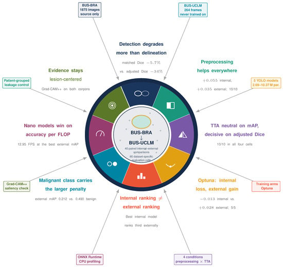
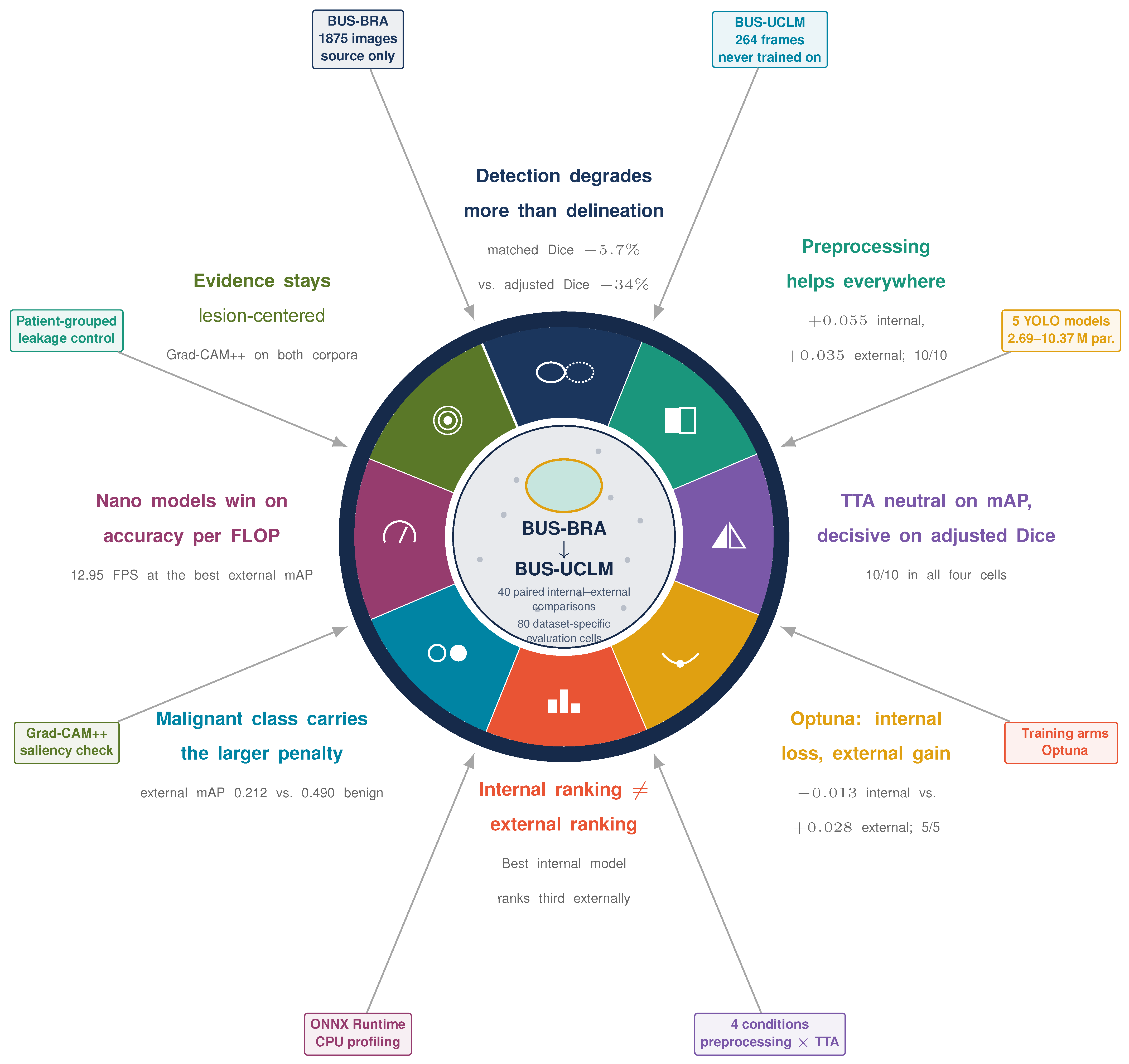
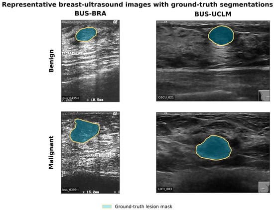
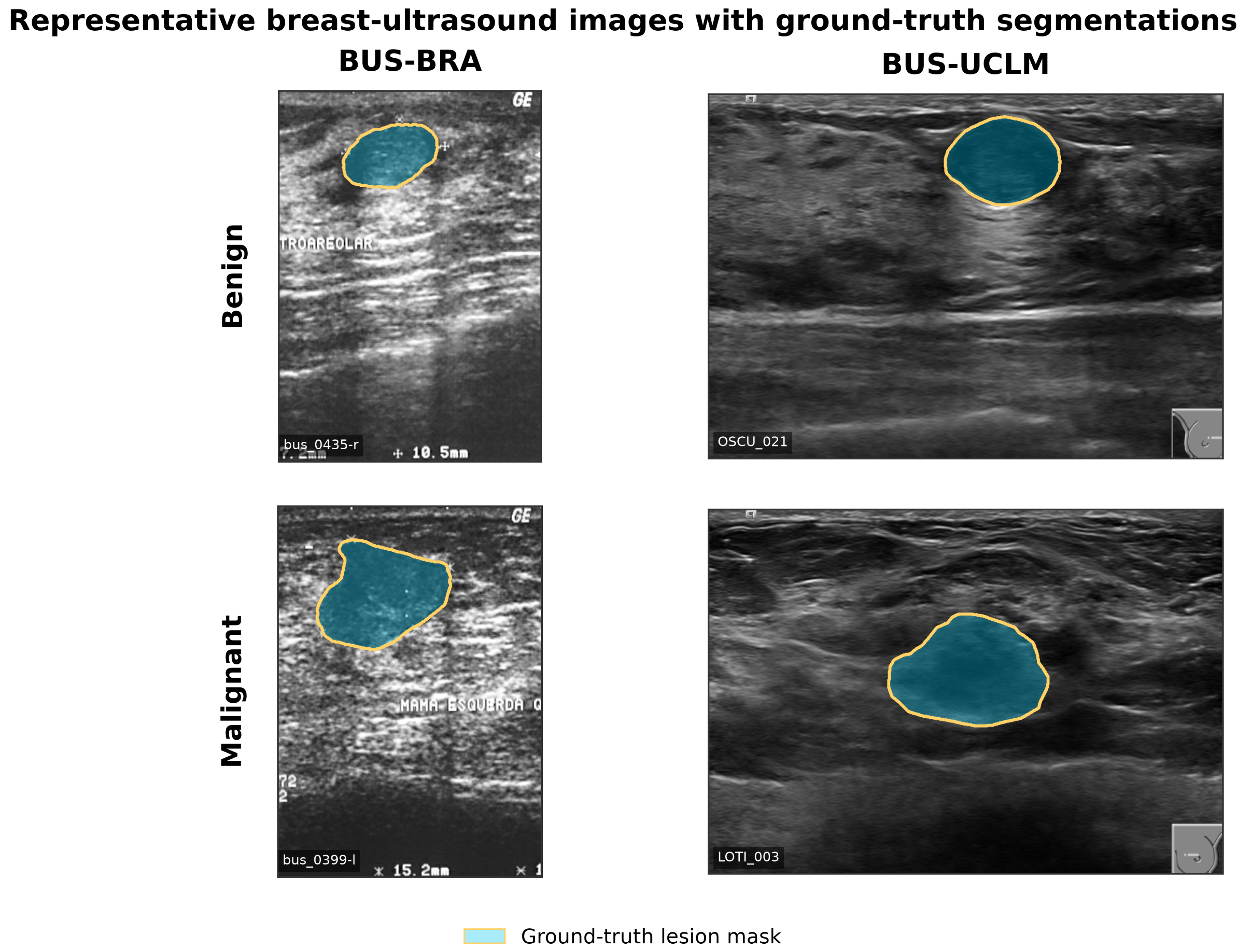
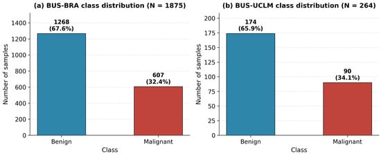
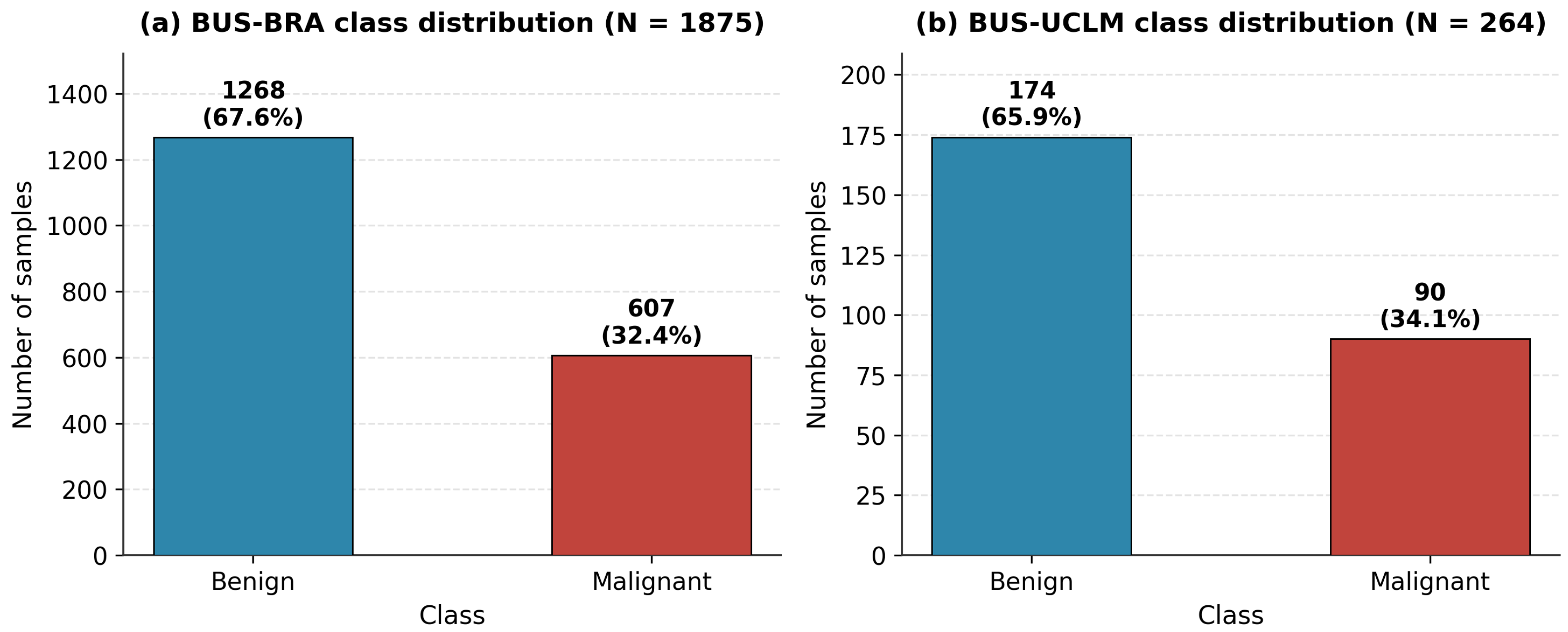
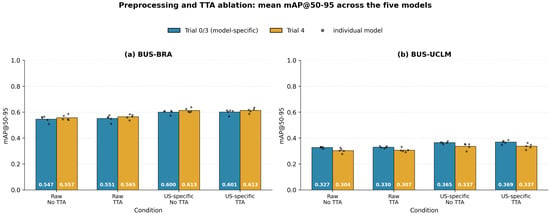
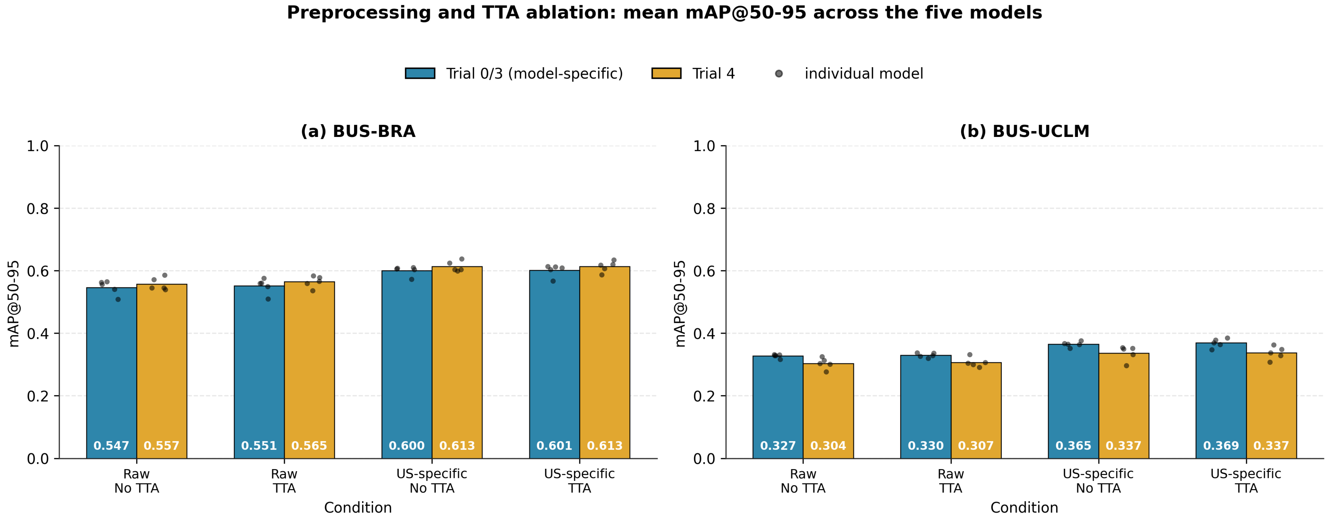
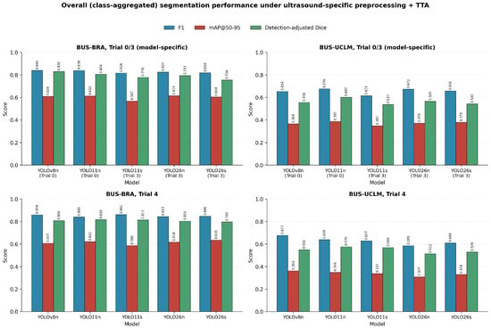
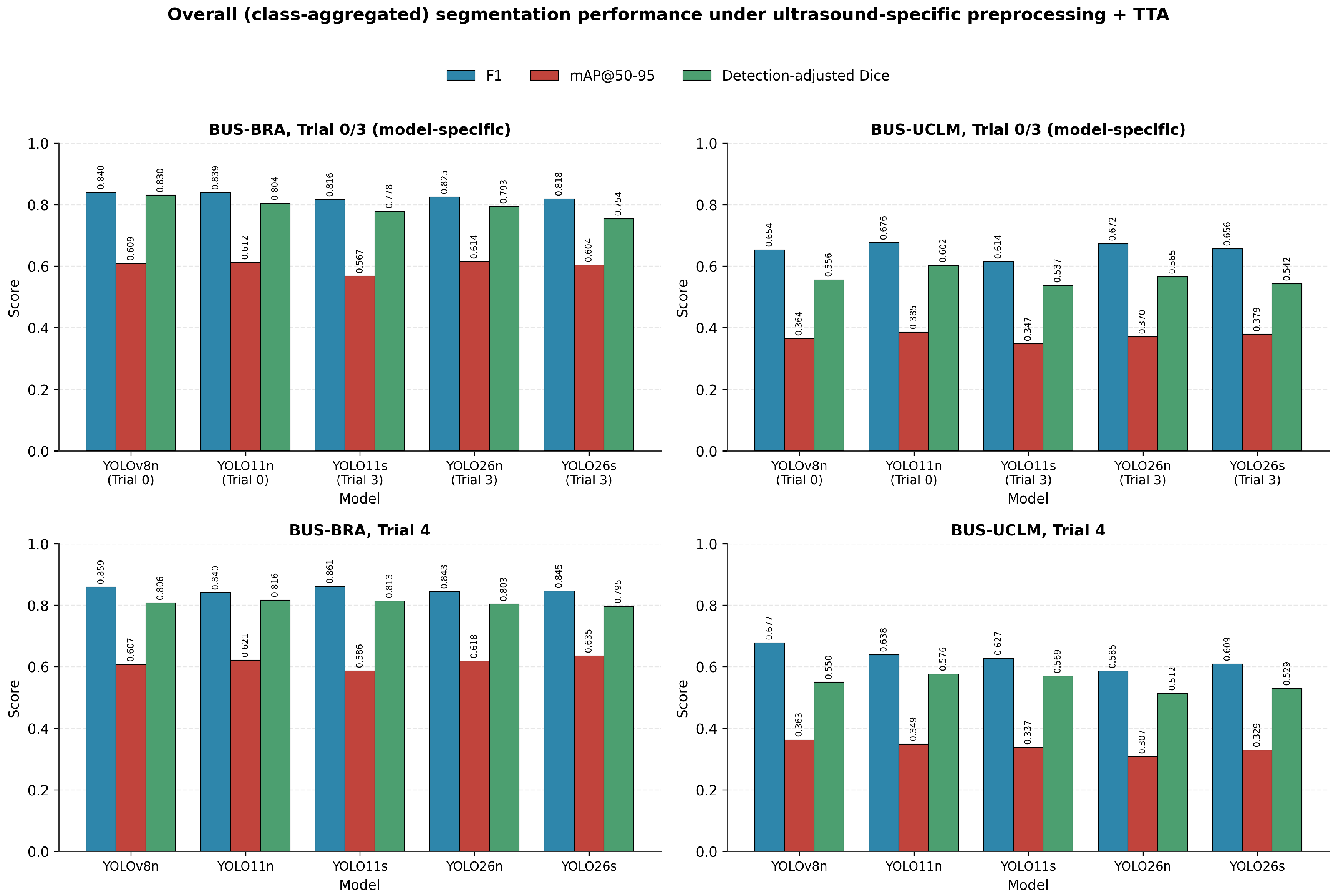
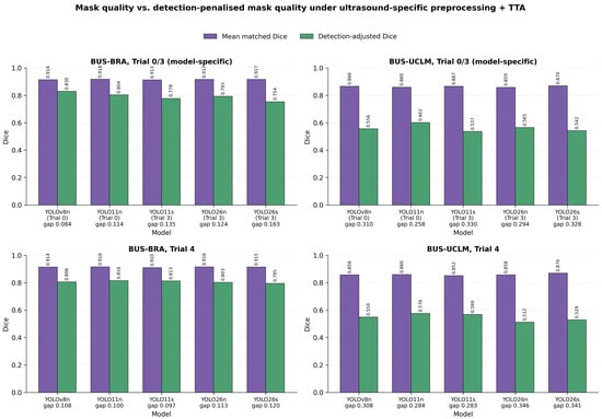
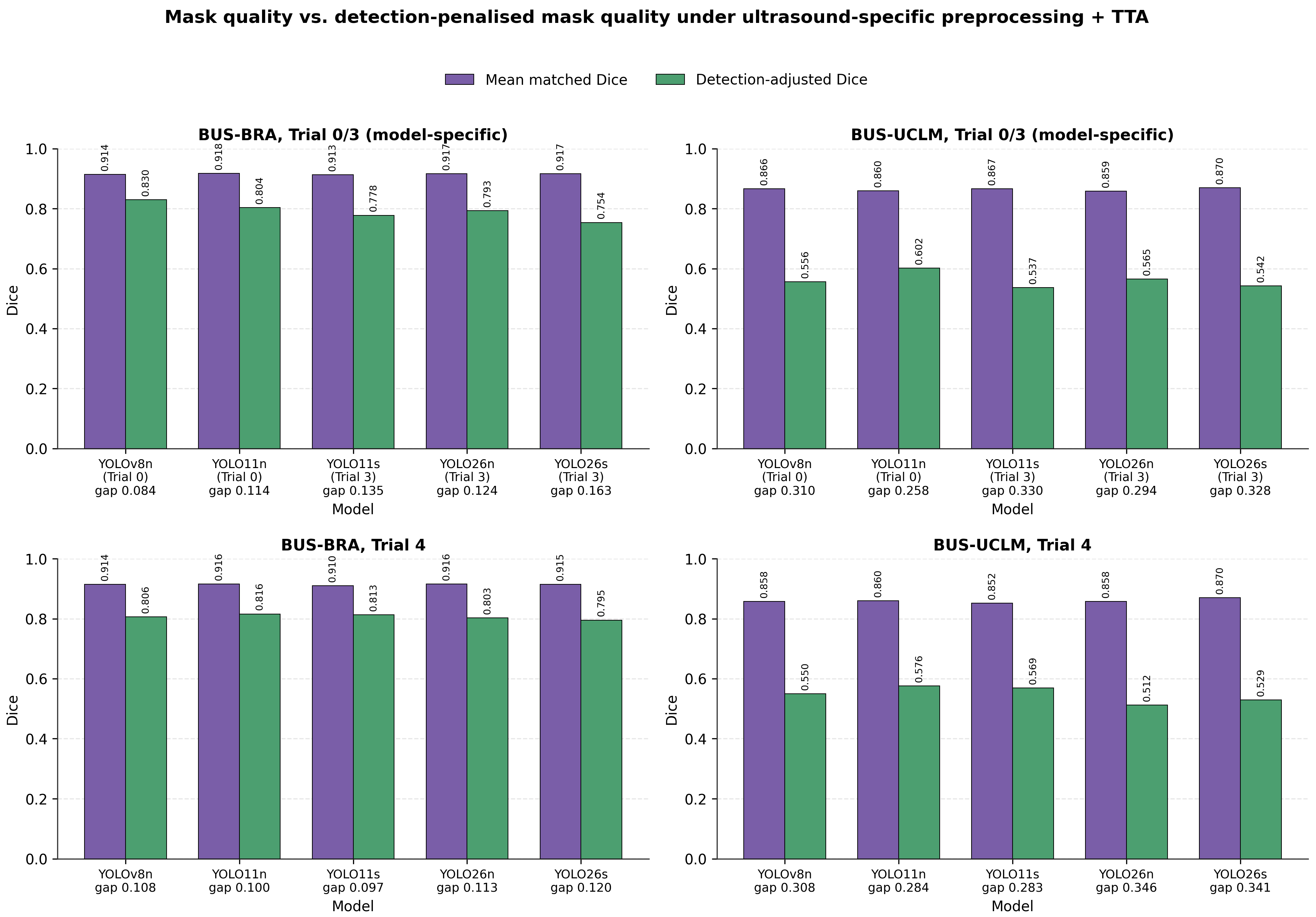
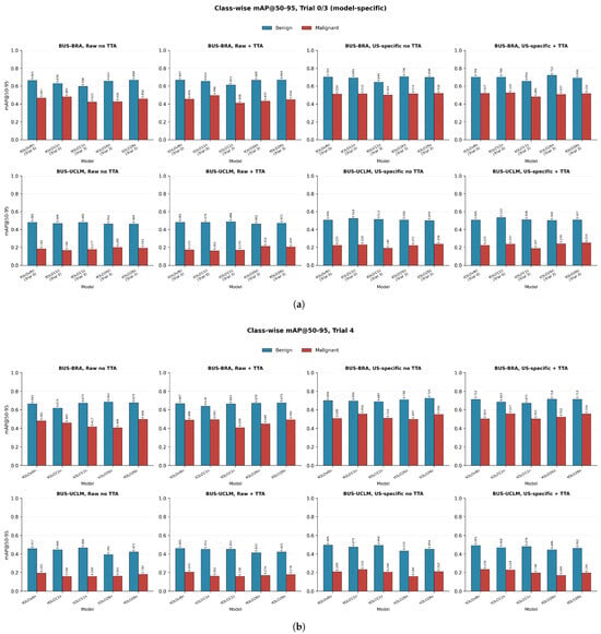
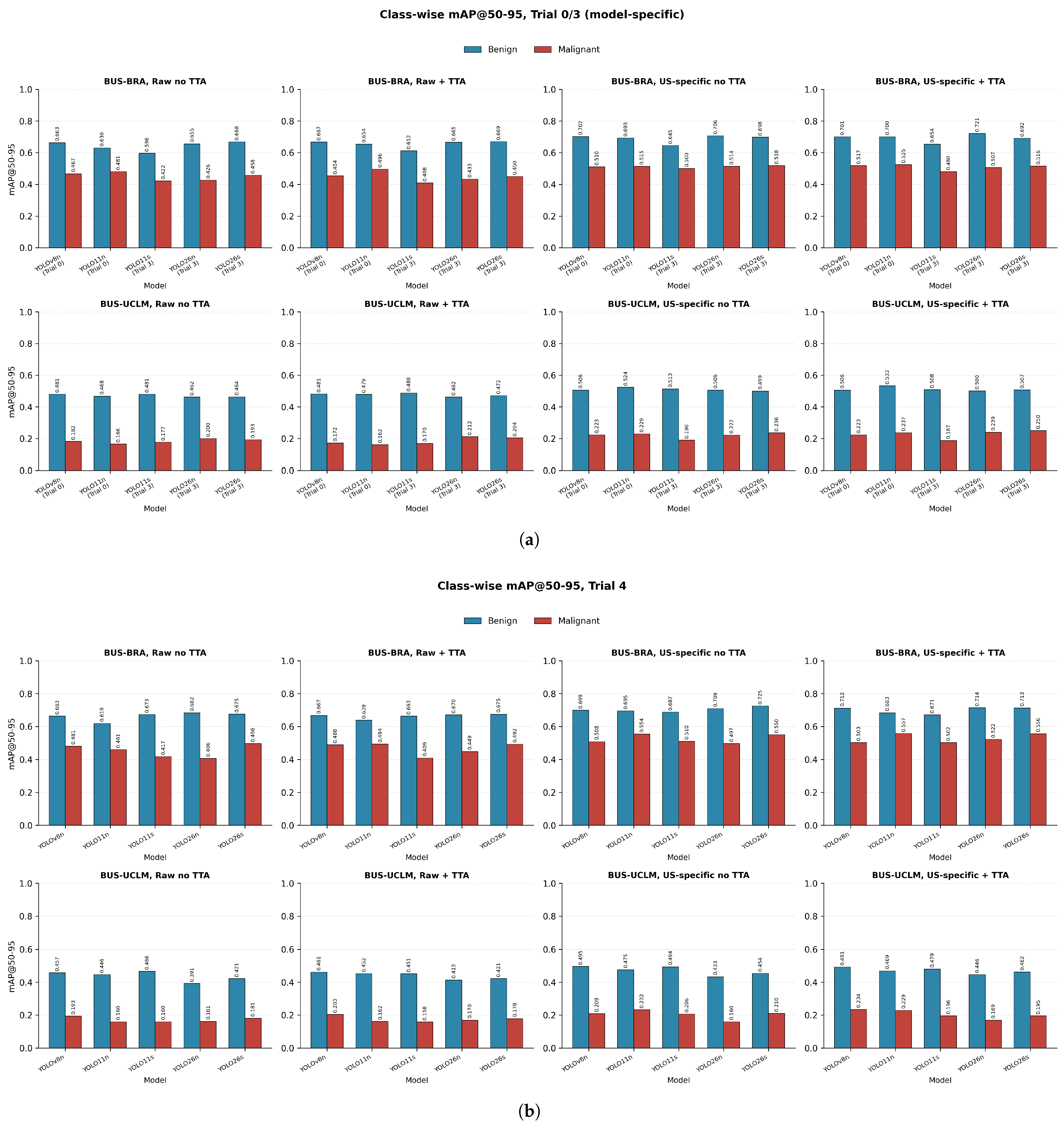
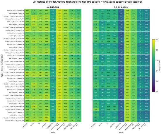
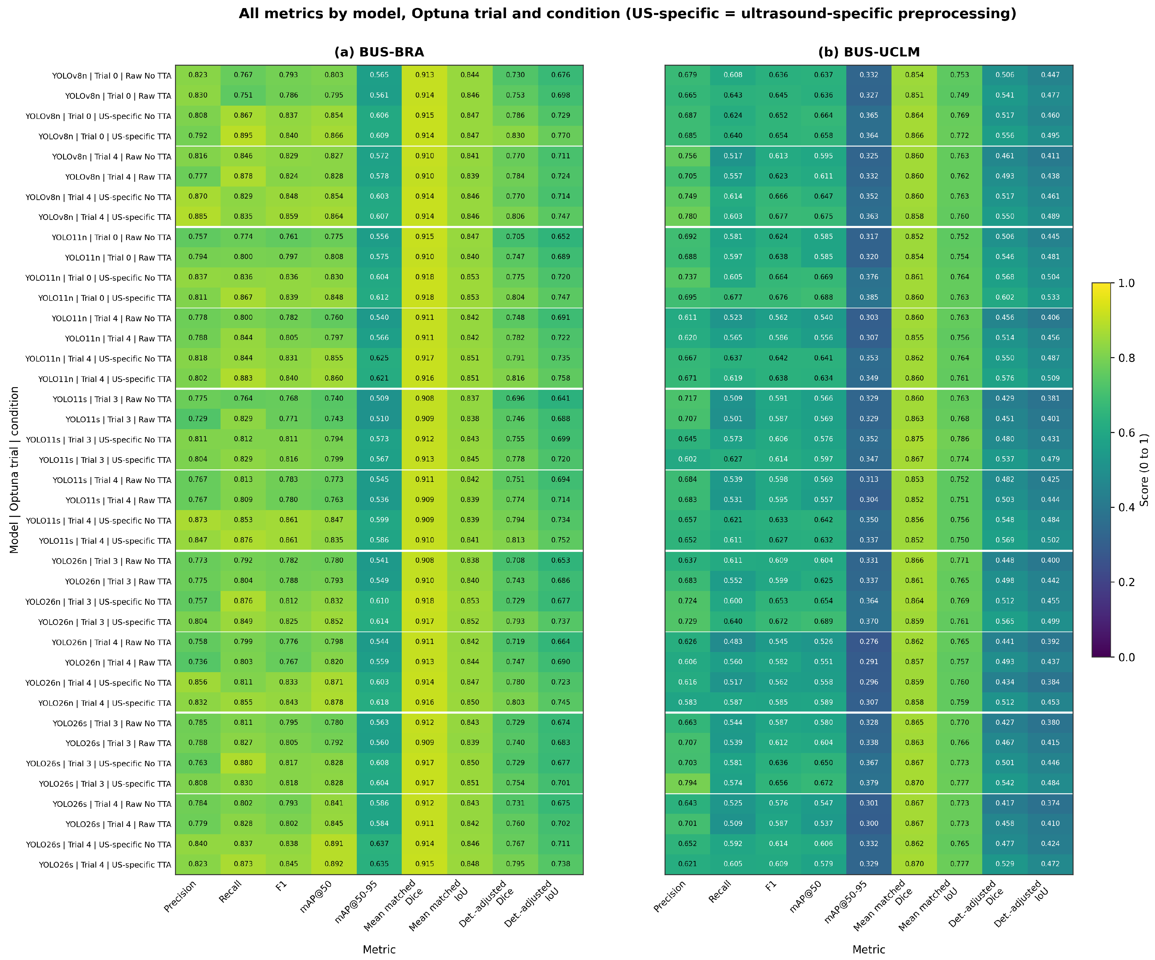
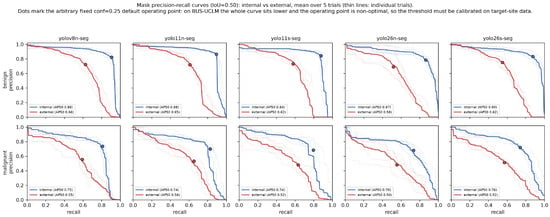
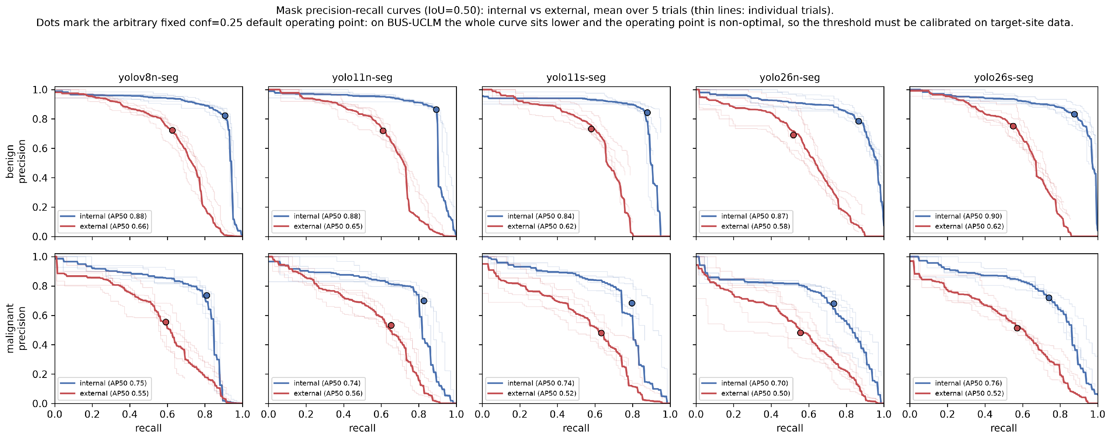
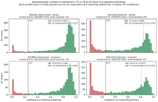
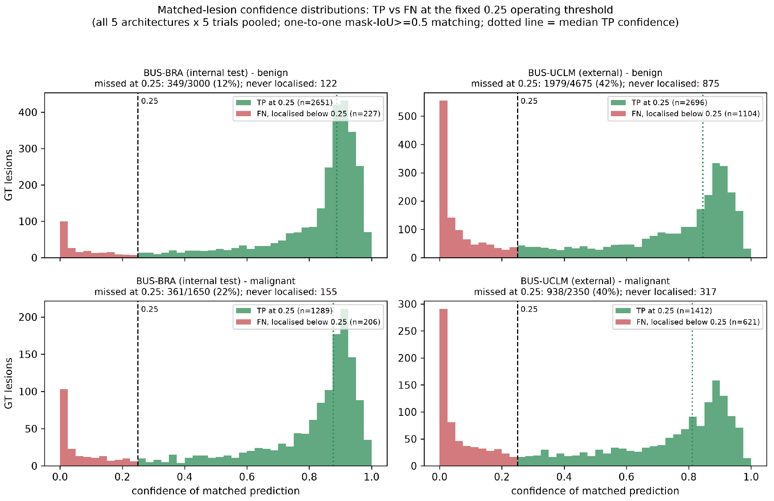
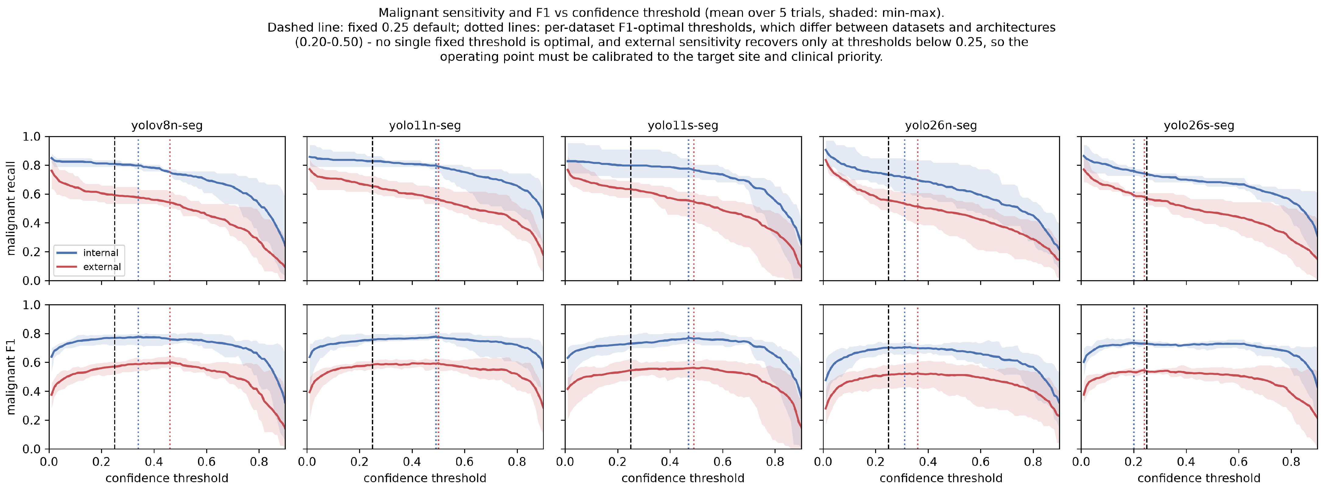
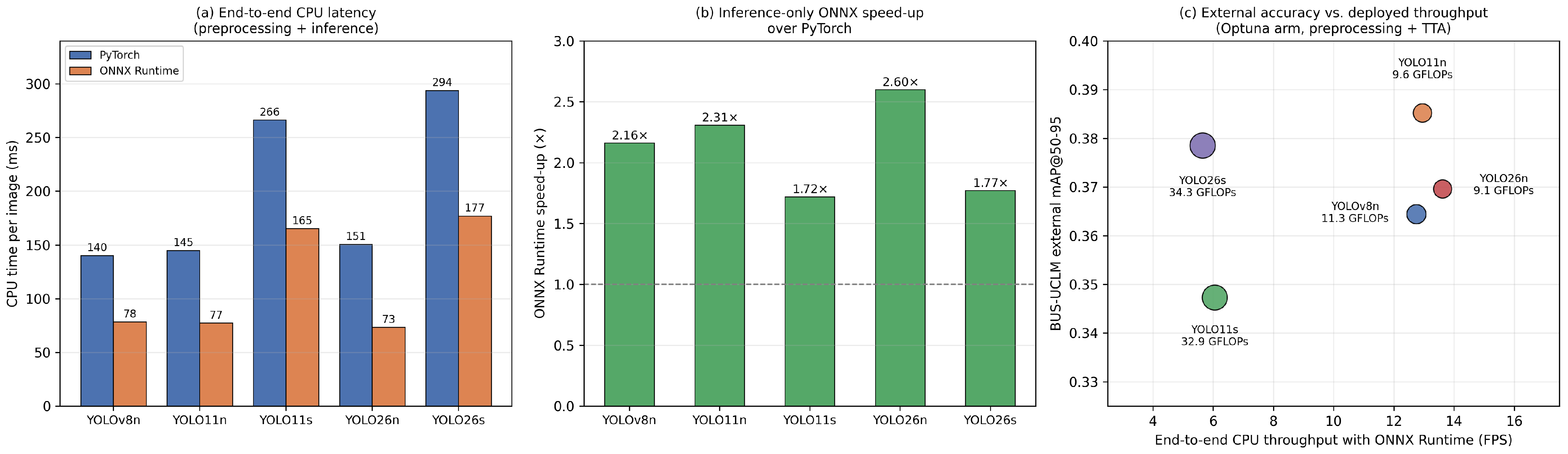
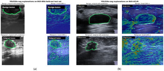
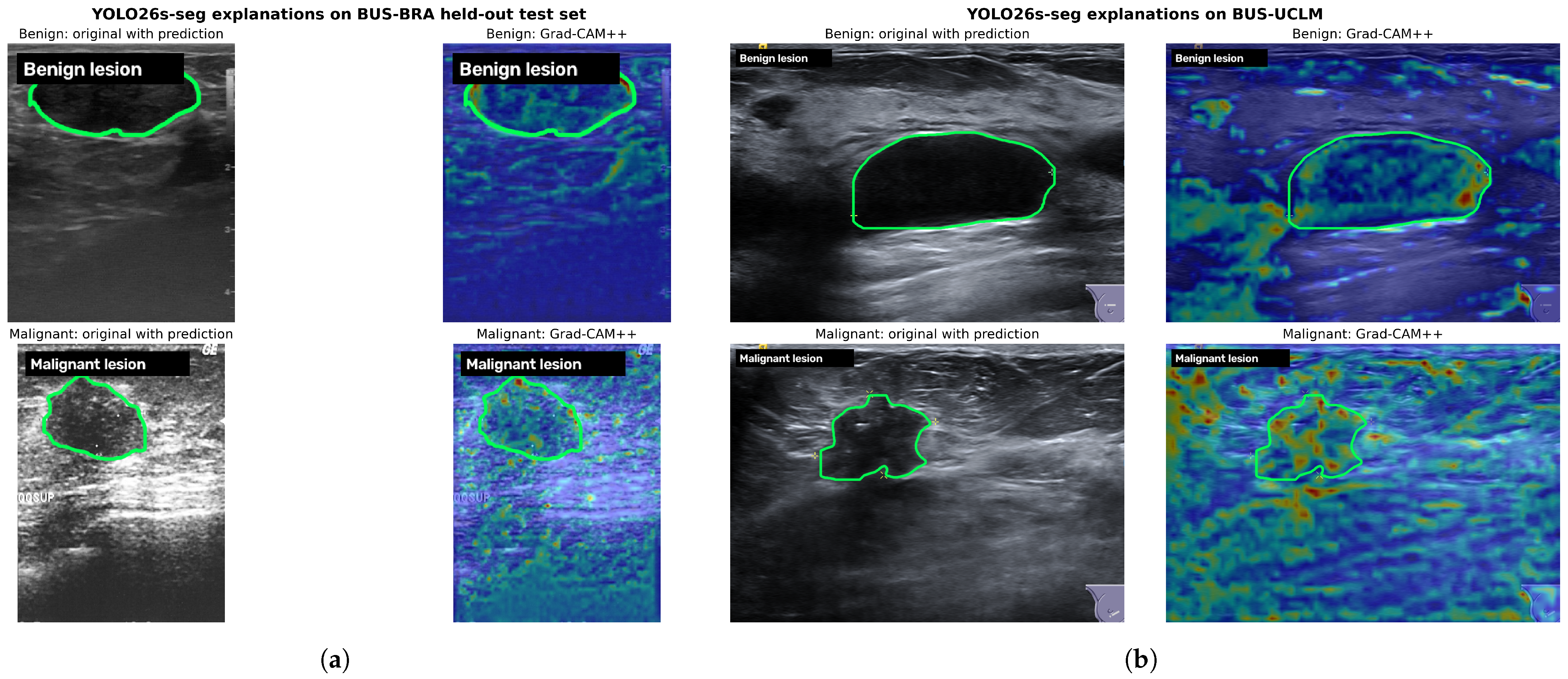

Disclaimer/Publisher’s Note: The statements, opinions and data contained in all publications are solely those of the individual author(s) and contributor(s) and not of MDPI and/or the editor(s). MDPI and/or the editor(s) disclaim responsibility for any injury to people or property resulting from any ideas, methods, instructions or products referred to in the content. |
© 2026 by the authors. Licensee MDPI, Basel, Switzerland. This article is an open access article distributed under the terms and conditions of the Creative Commons Attribution (CC BY) license.