


Abstract
This article presents analytical approaches for determining the stress state in hypotrochoidal profiles (H-profiles) under torsional, bending, and shear loading. The focus lies on shear loading. Using conformal mapping, a formulation of elasticity theory is first adapted to H-profile cross-sections. Closed-form solutions for the respective stress components are then derived by solving a reformulated surface integral. Suitable conformal mappings for hypotrochoidal contours are obtained through a successive method applied to their parametric description. These mappings are essential for the elasticity-theoretical formulation used to determine the stress state in the profile bar. Building on this, the transverse shear stresses for H-profile cross-sections are determined for the first time. The influence of shear stresses on the overall stress state is discussed in detail. These stresses generally act in a rotational manner and superimpose on the torsional stresses. This effect proves more pronounced here than in circular cross-sections. Accompanying finite element analyses (FEA), carried out for several examples, showed very good agreement with the analytical solutions. From the resulting maximum stress values and stress gradients, form and notch factors are calculated. The proposed procedure also applies to combined loading cases. It is intended for use in the new standard covering hypotrochoidal profile contours.
1. Introduction
Non-circular profile contours generally have a higher load-bearing capacity compared with traditional key and spline connections. This is due to lower notch numbers for both torsional and bending loads. In addition, closed stress solutions can be derived for many practical applications due to the continuous contour geometry [1,2,3]. Such solutions enable the reliable and cost-effective design of profile shafts.
In addition to the already known P3G profile according to DIN 32711 [4], the DIN 3689—Part 1 [5] for the geometry of hypotrochoidal profiles (H-profiles) is an elegant solution for the current high demands on shaft–hub connections. This article aims to contribute to DIN 3689—Part 2 “Calculation and dimensioning”, which is currently still in the planning process.
As a rule, shear stress is neglected in comparison with bending stress in a beam or shaft subjected to shear force. However, this is only permissible for large length ratios () depending on the type of shaft bearing, where denotes the length and the diameter of the shaft. Therefore, the shear stress must be checked and adjusted if necessary (see [3]).
Furthermore, in most practical applications, the shear force acting on the shaft has a rotating character, and therefore the resulting shear stress does not remain constant but exhibits a pronounced dynamic, alternating (fatigue-relevant) character as the shaft rotates. Consequently, this shear stress must be treated as a stress amplitude in the corresponding fatigue calculation and must be explicitly taken into account in the design of the shaft, since it acts directly on—and superimposes with—the torsional shear stress. Current standards and calculation regulations for round cross-sections do not account for this effect, as the shear stress is typically neglected or, at best, considered only as a static contribution.
In non-circular cross-sections, such as hypotrochoidal or H-profiles, this dynamic shear stress can play an even more significant role, since its interaction with the torsional stress has a stronger influence on the load-bearing behavior and fatigue strength of the profile than in the circular case [3].
2. Geometry
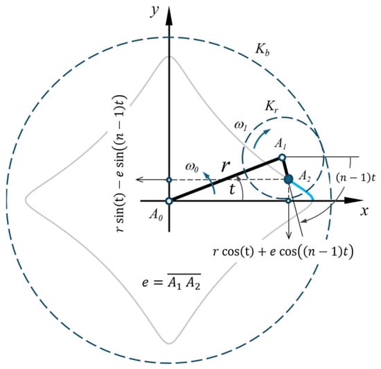
Hypotrochoids (H-profiles) belong to the so-called wheel lines [6,7] and are generated by rolling a circle on the inside of a fixed base circle . Figure 1 shows the generation principle of H-profiles. The distance between the generation point and the center of the rolling circle is referred to as the eccentricity of the profile. If the eccentricity is set to 0, and coincide, and the generated profile describes a circle parallel to the base circle. This means that the eccentricity describes the degree of the profile’s out-of-roundness.
Figure 1.
Definition of hypotrochoid.
For technical applications, closed curves with periodic symmetry are generally useful. The following conditions apply here:
- -
- The angular velocities and are oppositely directed.
- -
- , and the diameter ratio of the two circles , where is arbitrary and an integer.
describes the periodicity of the hypotrochoids and, therefore, also represents the number of sides of the profile.
If the generating point lies on the circumference of the rolling circle , the path describes a limiting case in which the curve begins to intersect itself. In this case, the eccentricity is given by
Depending on the distance between the selected point and its own pivot point, the so-called extended or shortened higher trochoids can also be generated from Equation (1).
For a hypotrochoid with a flat point (on the flank), the following applies according to [8]:
The parameter representation of the H contours can be determined as follows based on the generation principle in Figure 1:
Here, denotes the nominal radius, denotes the eccentricity, and denotes the periodicity (number of sides). Equation (3) can be represented using complex numbers as follows:
where , and , with . The variable takes on values from to , where denotes the center and describes the profile contour.
Therefore, the contour geometry can be determined using a single “complex” Equation (4), which simplifies the investigation of the geometric–mechanical properties of the profile. Since the function conforms the edge of a unit circle to the profile contour, the complex formulation facilitates the geometric investigation of the profile. In [9], such formulations were also used to solve the torsion problem and, in [3], the transverse shear stress in epitrochoidal cross-sections.
3. Formulation of the Shear Stress
Shear stress can be caused by both shear force and torsional stress. However, the respective effects have different mechanisms. The shear stresses resulting from torsional stress have been described in detail in [9]; therefore, they will not be discussed in detail here. The general formulation for shear bending was presented in [1,2], based on the elasticity behavior of the material. The procedure described in [1] is presented in a more understandable way. However, this requires a complex shear function depending on the profile geometry. Based on the complex formulation, a general procedure was developed in [3] from a parametric profile description according to Equations (3) and (4). The procedure was applied to the so-called epitrochoidal contours for non-rotating shear forces.
3.1. A General Formulation
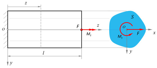
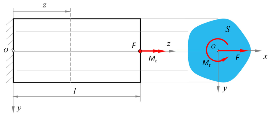
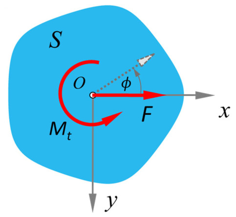
Based on the coordinate system for loaded cross-sections, as shown in Figure 2, the following formulation for stress components, according to [1], is used. Here, the shear force F is applied on the right side at the center of gravity of the cross-section and in the x-direction.
Figure 2.
Coordinate system for the loading of the H profile.
The first terms in Equations (5) and (6) provide the component of torsional stress resulting from a torsional function φ (see also [9]). The second terms determine the corresponding stress components due to shear force using a shear function . To solve the transverse shear stresses, only the shear force was considered in [3], and the second terms in (5) and (6) were included to derive the solution for the so-called epitrochoidal cross-sections. In addition, the direction of the shear force was fixed in the x-direction. In this work, the solution is extended to hypotrochoidal cross-sections (DIN 3689—Part 1). Furthermore, the effects of the rotating shear force are included in the solution. The combination of a torsional load with the rotating shear force is also considered. The third equation, Equation (7), is simpler and provides the bending stresses independently of φ and .
3.2. Method for the Solution
In this work, the solution is first extended to hypotrochoidal contours (H-profiles) used in DIN 3689—Part 1. The rotation of the shear force is also carried out in the solution using a rotation angle. To solve Equation (5) to (7), φ and must first be determined. However, these generally depend on the geometry of the profile contour; therefore, classical elasticity theory is not readily able to offer a general solution. There are solutions for some specific cross-sections such as circles, ellipses, etc. [10], which do not correspond to hypotrochoidal cross-sections.
However, if a conformal function based on the contour description can be found that can conformally map the entire cross-section onto a unit circle, the solutions to the two functions φ and are possible. For hypotrochoids, this is not possible due to multiple poles in the parameters in Equation (3) being determined directly. Therefore, to determine the appropriate mapping function, the successive method, according to Kantorovich [11], was used, as in [9].
3.3. Determination of Suitable Conformal Mapping for H-Profiles
Since the mapping obtained from the parameters in Equation (3) has poles (see [9]), it can map the circumference of the unit circle onto the profile boundary; however, the center point moves to infinity multiple times. Therefore, determining a suitable mapping is the first step.
The successive approximation method of Kantorovich [11] is a well-established technique for the iterative solution of nonlinear integral equations, such as those arising in the conformal mapping of eccentric contours onto a reference circle.
A related application of the successive approximation method for conformal mapping was presented by Lee [12], who investigated fibers with a hypotrochoidal cross section. Using complex variable techniques, he derived a conformal mapping function in power series form. From this function, the torsional constant and the bending moment of inertia were obtained in closed form. In contrast to the present work, however, this study focused on the stiffness properties of the cross section rather than on the resulting stresses.
Another method of Ivanshin and Shirokova [13] provides an approximate conformal mapping of the unit disk onto a simply connected domain with smooth boundary, obtained directly as a Taylor polynomial by solving a Fredholm integral equation of the second kind for the boundary reparameterization, without requiring auxiliary constructions or iterative procedures.
Although both methods avoid iterative schemes and reduce the mapping problem to a finite linear system, they differ in series efficiency. The Kantorovich method yields accurate solutions already at low orders () for near-circular domains, as its basis functions are inherently well-suited to small eccentricities. The Ivanshin–Shirokova method, by contrast, expands the mapping as a Taylor polynomial without exploiting circular proximity, requiring considerably higher orders () to achieve comparable accuracy in the reported hypotrochoidal example. Its main advantage therefore lies not in series efficiency but in avoiding the construction of a domain-specific orthogonal basis. However, when the resulting mapping function is subsequently used to solve the associated elasticity problem, such high-order series become impractical, as they lead to correspondingly large equations.
In this work, the Kantorovich method was therefore employed to approximate the mapping function that maps the unit circle onto the hypotrochoidal cross-section, assuming a series of epitrochoidal character—that is, with positive exponents of ζ—in the mapping function. The application of this approach is explained in detail in [9].
3.4. Approximate Method After Kantorovich
From the parameter equation, Equation (4), a mapping for the profile boundary curve can always be derived directly. This mapping can serve as a starting point for approximating the mapping sought here. In general
On this basis, the complex form of the mapping function can be expressed as
where denotes the parameter angle and the principal eccentricity of the profile. The boundary curve can then be expressed in the complex form , where denotes Euler’s number (not to be confused with the profile eccentricity).
It is evident from the equation that, due to the negative sign of , the function has multiple poles and is therefore not suitable for a complete mapping.
Since, in general, the parameter does not coincide with the polar angle in the model plane, a relationship between and is assumed in the form of the following series:
in which are periodic real functions of still to be determined. Substituting (10) into (9) yields the following mapping function:
Expanding this function in a Taylor series about the point yields the following general form for the individual terms in (16):
When these individual terms are substituted into Equation (9), the following general form of the mapping function is obtained:
in which the factors are computed from Equation (12) as follows:
A suitable choice of the functions allows the appropriate mapping for the profile cross-section to be determined. For the mapping function, the following conditions are to be satisfied by the functions:
- -
- .
- -
- All negative exponents in the mapping function are eliminated.
This yields the general form:
Starting from the parametric representation (4) of the hypotrochoidal contours, the following mapping is obtained:
The mapping function (16) does not provide a proper conformal mapping of the unit circle onto the cross-section enclosed by the hypotrochoidal contour. Nevertheless, this function is suitable for the successive approximation of a complete and appropriate mapping and is therefore taken as the basis for the following considerations. The ff-functions can be determined as follows with the aid of Equations (13) and (14):
Equation (17) shows that raising the series order of the mapping function can cause the corresponding equation length to grow rapidly. Furthermore, numerous investigations have shown that beyond a certain limit—dependent on the profile eccentricity and the number of —increasing the approximation order no longer yields any improvement.
3.4.1. Kantorovich’s Convergence Analysis
Kantorovich [11] carries out a convergence analysis of his successive method and establishes convergence for small values of the eccentricity e. He leaves the exact radius of convergence undetermined, however, recommending instead that the usability of the resulting approximation be verified a posteriori, i.e., once the mapping function has been determined [11]. It is shown here, though, that the actual convergence limit for may, depending on the application, lies above the bound proven by Kantorovich—a finding also reported in [9]. The results presented in the following sections should accordingly be read as an extension, rather than a contradiction, of Kantorovich’s original analysis: they indicate that his sufficient condition for convergence is, in practice, often conservative.
Convergence Behavior at Low Eccentricity
For contours of low eccentricity, the successive method exhibits, as expected, excellent convergence behavior, since at low eccentricity the deviation from a circular shape is small and the higher-order perturbation terms decay correspondingly fast. In this range, the series expansion converges not only rapidly but also uniformly, so that even low approximation orders are sufficient for a practically adequate description of the contour.
Convergence Behavior at Medium Eccentricity
As eccentricity increases, the convergence behavior of the method deteriorates noticeably at first. In the medium eccentricity range, however, a good approximation quality can still be achieved by deliberately increasing the number of series terms. Convergence here proceeds considerably more slowly than in the low-eccentricity range yet remains fundamentally stable: a higher order of approximation compensates for the growing influence of the nonlinear perturbation terms, allowing the numerical solution to approach the exact contour successively. The computational effort required in this range increases noticeably, since a satisfactory accuracy is only reached at a higher number of terms.
Occurrence of Local Irregularities at High Approximation Order
A more detailed examination shows that, while increasing the number of series terms improves the representation of the contour character, it simultaneously gives rise to new, undesirable effects. As the approximation order increases, locally irregular points form along the computed contour, attributable to oscillatory disturbances associated with the higher-order series terms. On further increase in the number of terms, these local instabilities spread and can subsequently lead to contour self-intersections—the approximated contour thereby loses its geometric consistency and becomes physically and geometrically inadmissible. This behavior points to a practical limit on the useful approximation order: an unbounded increase in the number of series terms does not improve convergence monotonically but instead leads, beyond a critical order, to a degradation of solution quality.
3.4.2. Practical Strategy for Limiting the Size of the Resulting Equations
Parameter studies with varied values of the number of series terms and the eccentricity identified a strategy that offers a good compromise between the size of the resulting equations and the achieved approximation quality. In this approach, the number of series terms is initially chosen deliberately high— was adopted in the present work—in order to capture the convergence properties of the method as fully as possible. For the subsequent derivation of the equations used for stress calculation, however, only a considerably smaller number of the leading series terms is retained; in the present work, these are the first four terms. In this way, the size of the stress equations required later is substantially reduced, without essentially losing the approximation quality previously secured through the higher number of terms.
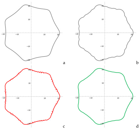
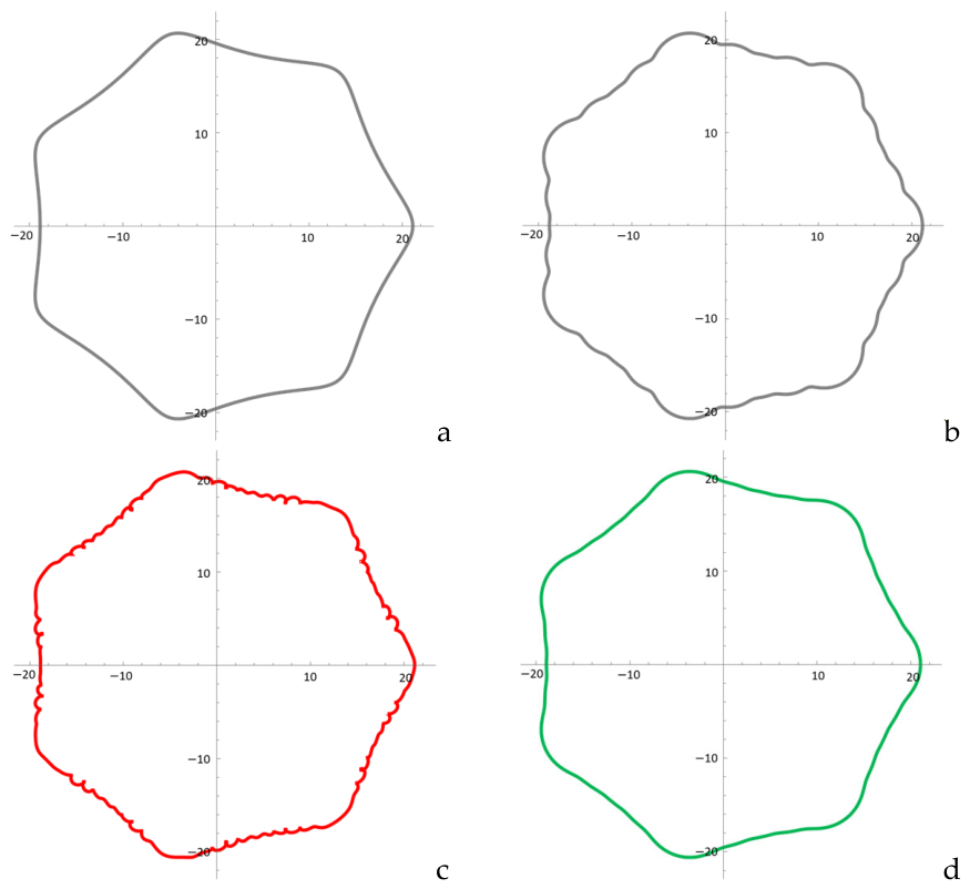
Figure 3 illustrates this trade-off for the example of an H-profile with , and . Figure 3a shows the exact target contour. Figure 3b shows the approximation obtained with a 4th-order series, which exhibits clearly recognizable local as well as global shape deviations. Figure 3c, bottom left, shows the approximation obtained with a 14th-order series; although the global approximation—i.e., the overall contour, or profile character—is improved, several locally irregular points and self-intersections form along the profile contour. The approximation proposed in this work, obtained with a series truncated to the leading coefficients, is shown in Figure 3d; here, both the global and the local approximation are captured well.
Figure 3.
Comparison of the approximation quality for an H-profile with , and e = 1.15 mm. (a) exact target contour; (b) 4th-order approximation; (c) 14th-order approximation; (d) approximation with series truncated to the leading coefficients (present work).
3.5. Determination of the Mapping Coefficients
As discussed above, increasing the approximation order improves the accuracy of the solution along the profile flanks and corners but disturbs the overall solution in the intermediate regions. At the same time, a larger number of terms in the approximation function results in very extensive solution equations, which makes the practical application of the results costly. In order to achieve a sufficiently accurate approximation while keeping the size of the equations within reasonable limits, an approximation order of 14 was initially selected, of which only the first four coefficients were retained for the solution. The conformal mapping function is determined as follows:
The above coefficients were found based on [9] as follows:
Rotating load
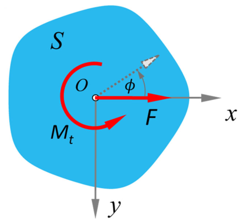
To analyze the shear stresses, the coordinate origin is placed at the centroid of the profile’s cross-section, as shown in Figure 4. To include the rotation of the cross-section in the formulation, a force angle is included, as shown in Figure 3, which has a minus sign in the mapping function. This is because it is the cross-section that rotates and not the force. Equation (18) therefore takes the following form:
Figure 4.
Implementation of the force angle for a rotating cross-section.
3.6. Approach for Determining
First, a function , conjugate to for the profile, is determined from the boundary condition on the profile contour as follows [1]:
Due to the closed profile contour, the constant value disappears on the right side of Equation (15). If the function is known, and can now be determined using Cauchy’s integral formula.
If the contour geometry was described by parameter equations with cos and sin terms (e.g., Equation (3)), the cos and sin functions are first rewritten as expressions of
where e is Euler’s number. This gives Equation (24) the following parametric form:
λ is the edge of the unit circle and corresponds to the profile contour in the real plane. According to [1], a function , conjugate to , can first be determined for the profile contour from the boundary condition (the cross-section is load-free at the edge) as follows:
Based on this, and can then be determined using Cauchy’s integral formula:
is the real part of the complex bending stress function from Equation (30) in the so-called model or ζ plane and can, therefore, be determined from . The stress components for the shear force can then be determined using the following equations:
For the partial derivatives of occurring in Equation (31), is also required:
where , and denote the corresponding derivatives according to parameter .
is the moment of inertia around the y-axis and can be determined from the following relationship:
As shown in [14,15], remains independent, due to the periodic symmetry of the force angle ϕ.
3.7. Approach for Determining φ
First, the function , conjugate to for the profile contour, is determined from the boundary condition on the profile contour as follows [1]:
denotes the conjugate function of , obtained by replacing with .
Based on this, or φ can then be determined using Cauchy’s integral formula.
Due to the closed profile contour, the constant value disappears on the right-hand side of Equation (35).
is the real part of the complex torsion function from Equation (35) in the model plane and can therefore be determined from . The stress components for the torsional load can then be determined using the following equations:
If we now combine the respective stress components from Equation (36) with Equation (31), we obtain Equations (5) and (6) again.
4. Application to H-Profile
To illustrate the contour approximation procedure more clearly, the method is applied to specific test examples from DIN 3689—Part 1 [5], and the results of the corresponding stress distributions are compared with the FEA results.
It should be emphasized that the analytical approach presented in this work is not restricted to the two specific profiles selected as illustrative examples. Rather, the underlying conformal mapping and the resulting closed-form stress solutions are formulated in general terms as a function of the governing geometric parameters of the hypotrochoidal profile family defined in DIN 3689. Consequently, the methodology is directly applicable to the entire range of standardized profile configurations covered by this standard, and the two selected examples merely serve to demonstrate and validate the general procedure.
To illustrate the application of the proposed methodology, two representative standardized profiles are considered in the following, differing in their geometric parameters and in their eccentricity.
Examples
Two cases with four and seven sides were selected from the standard DIN 3689—Part 1 and examined. Table 1 shows the designation, the geometric dimensions, and the coefficients determined from Equation (19) to (23) for the mapping function.
Table 1.
Profile examples from the standard.
Based on this, the approximated mapping functions can be determined as follows:
for H4−40 × 35.79 and
for H7−40 × 37.84.
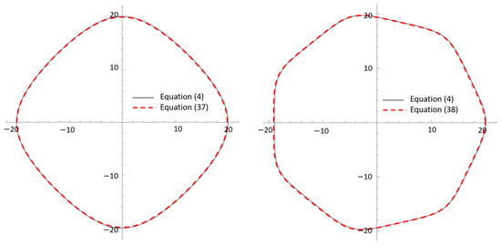
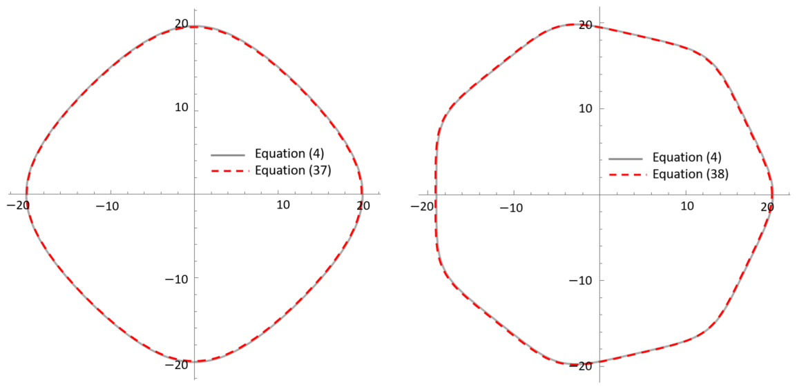
Figure 5 compares the approximated and exact profile contours for profiles with four and seven sides. In both cases, the results show excellent agreement, confirming the validity of the proposed approximation.
Figure 5.
Match between the contour approximation Equation (37) or (38) and the exact contour according to Equation (4), (left) for H4−40 × 35.79 and (right) for H7−40 × 37.84.
The observed agreement is disrupted with increasing eccentricity. It should be noted that Equations (4) and (37) or (38) are equivalent regarding contour mapping. However, Equation (37) or (38) is suitable for the complete mapping of the cross-section, as no infinite poles occur here.
To include the rotation of the shear force, the mapping function is multiplied by :
for H4−40 × 35.79, and
for H7−40 × 37.84.
Calculation of stress components
Substituting Equations (27) and (28) into Equation (29) with coefficients for H4−40 × 35.79 from Table 1 yields the corresponding for the profile edge (at ). Based on this, the bending function can be determined from Cauchy’s integral formula (30) and as the real part of . Finally, can be used to calculate the stress components from Equation (31). For a transverse contraction ratio and a bending angle , the following stress components are determined for the profile contour of H4−40 × 35.79:
In addition to the analytical approaches presented above, finite element analyses (FEA) were carried out to validate and complement the analytical results. The results of the FE simulations are subsequently compared with the analytical predictions to evaluate their accuracy and applicability.
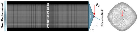
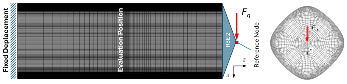
The finite element analyses were carried out using the MSC-Marc software system 2020. Figure 6 illustrates the mesh structure and corresponding boundary conditions, using the example of H4-40 × 35.79. The profiled shaft is clamped on its left-hand side, while the transverse force is transmitted to the right-hand side via a reference node using an REB2 element. The resulting FE mesh comprises 564,192 fully integrated hexahedral elements (type 7 according to the Marc Element Library [16]) and an equal number of nodes. The meshes were generated using in-house software developed in Python 3.12 at the Chair of Machine Elements at the West Saxon University of Applied Sciences in Zwickau and were subsequently imported into MSC-Marc for further pre-processing.
Figure 6.
FE mesh and boundary conditions for the H-profile with four sides H4−40 × 35.79.
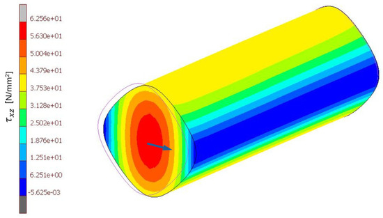
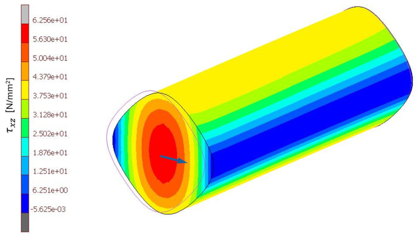
Based on this model, the shear stresses resulting from the applied transverse force were subsequently evaluated. Figure 7 shows the 3D shear stress distribution obtained from the finite element analysis.
Figure 7.
Three-dimensional distribution of shear stress due to transverse force H4−40 × 35.79 for and kN, (FEA results). Arrow: transverse shear force.
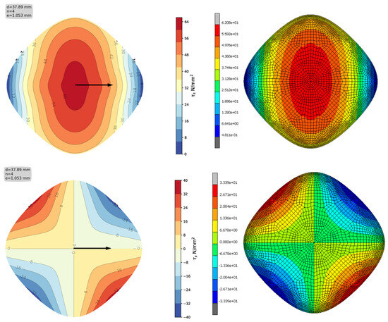
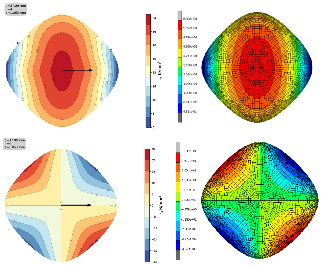
Figure 8 shows the respective distribution across the entire cross-section. A comparison with the analytical results shows very good agreement, thereby confirming the validity of the analytical approach.
Figure 8.
Comparison of the results of stress components (top) and (bottom) with the FEA outcomes, for and kN. Arrow: transverse shear force.
The resulting shear stress is then calculated using the following equation:
The bending moment of inertia is calculated using the data from Table 1 and Equation (22) .
Substituting any other values for into Equation (39), one obtains the corresponding stress components in the same way. For example, the following equation, Equation (44) gives the stress component with :
Figure 9 shows the distribution of the resulting shear stress (left) and (according to Equation (44)) on the profile cross-section with for a shear force .
Figure 9.
Distribution of the resulting shear stress (left) and (according to Equation (44)) (right) on the profile cross-section for and . Arrow: transverse shear force.
By substituting Equations (27) and (28) into Equation (29) with coefficients for H7−40 × 37.84 from Table 1, the stress components can be determined in the same way. For a transverse contraction factor ν = 0.3 and a bending angle , the following Equation (34) for is determined for the profile contour ():
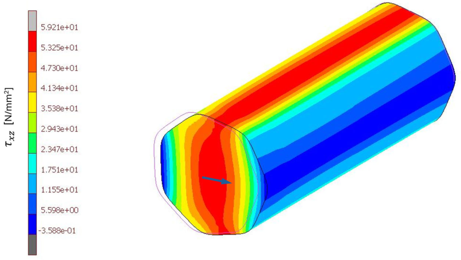
To further verify the analytical approach, a second example with a different geometric configuration was investigated. Figure 10 shows the corresponding shear stress distribution obtained from the finite element analysis.
Figure 10.
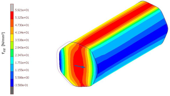
Three-dimensional distribution of shear stress due to transverse force for and kN, H7−40 × 37.84 (FEA results). Arrow: transverse shear force.
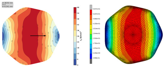
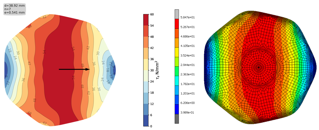
Figure 11 shows the distribution of on the cross-section of profile H7−40 × 37.84, with the analytical solution (left) and the numerical FE analysis (right) showing good correlation. The shear force here is .
Figure 11.
Distribution of shear stress in the cross-section of H7−40 × 37.84 (analytically, left) and FEA (right) for , and Arrow: transverse shear force.
The comparison with the analytical predictions again shows very good agreement, thereby further substantiating the validity of the analytical approach across different geometric configurations.
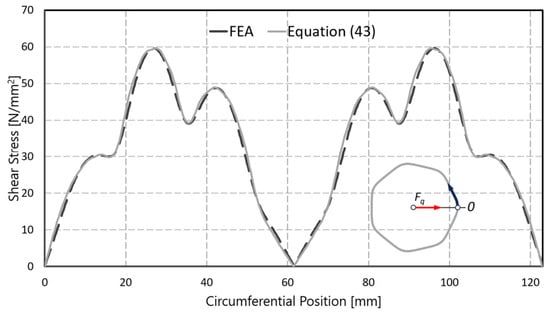
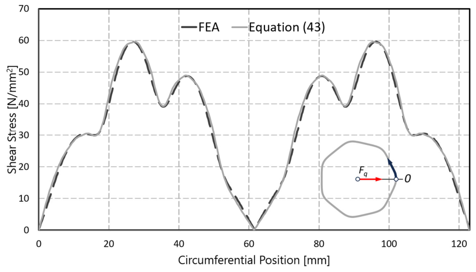
For a more detailed comparison of the results, the resultant shear stress was determined according to Equation (43) and evaluated along the profile contour for H7−40 × 37.84. The corresponding distributions are summarized in Figure 12.
Figure 12.
Comparison of the resulting shear stress distribution along the profile contour obtained analytically (Equation (43)) and by FEA for H7−40 × 37.84 for , and
To quantify this agreement, the relative deviation between the analytical and finite element results—normalized with respect to the global maximum shear stress obtained from the FEA—was evaluated. The maximum deviation amounts to approximately 7.0%, occurring on a rising flank of the stress distribution (tangential position ≈ 73 mm), where the absolute stress level is comparatively low. Near the governing maximum shear stress (tangential position ≈ 27 mm), the deviation is below 0.2%. Averaged over the entire circumferential position, the mean and RMS deviations amount to approximately 1.7% and 2.4%, respectively, confirming the very good agreement between the analytical and finite element solutions.
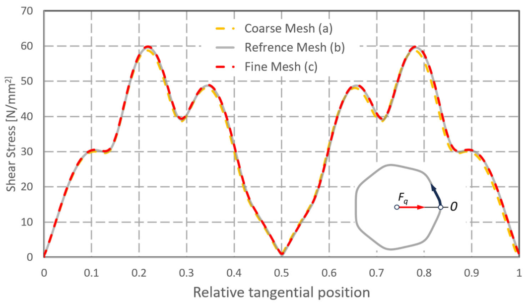
A mesh convergence study, detailed in Appendix A, verifies that the finite element results presented above are effectively independent of further mesh refinement. Figure A1 presents the three FE meshes considered for the H7−40 × 37.84 profile, namely a coarse mesh, the reference mesh, and a fine mesh. As evidenced in Figure A2, the corresponding results show only negligible discrepancies.
Bending stress:
The bending stress can also be easily determined from the last equation in (31):
where is defined as follows:
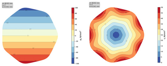
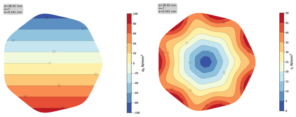
The left-hand side of Figure 13 shows the distribution of the bending stress according to Equation (35) for profile H7−40 × 37.84. An angle of was used here.
Figure 13.
Distribution of the bending stress (left) and torsional stress (right) in the cross-section of the H7−40 × 37.84 profile for , Fq = 50 kN, and Mt = 500 Nm.
Torsional stress:
The torsional stress on non-circular profiles was discussed and described in detail in [9]; therefore, it will not be addressed in detail here. The mapping functions derived according to Equation (18) also work for torsional stress. Since this is an axially symmetric load, the application of the mappings according to Equation (24) is not urgent. The right-hand side of Figure 13 shows the distribution of torsional stress in the cross-section for profile H7−40 × 37.84 applying (38) as a mapping function.
Combining torsion with a rotating shear force
In this case, the shear force will have a dynamic character and will be superimposed with torsional stress, occurring as medium stress:
This means that the transverse shear stress represents the stress amplitude and should therefore not be neglected when dimensioning the profile shaft.
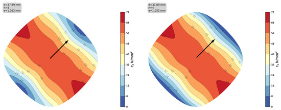
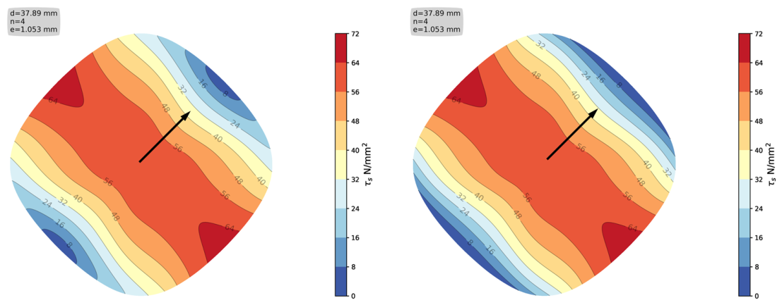
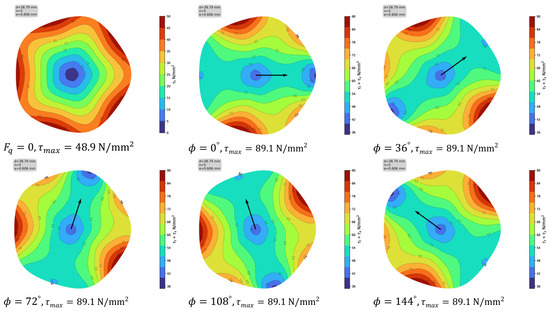
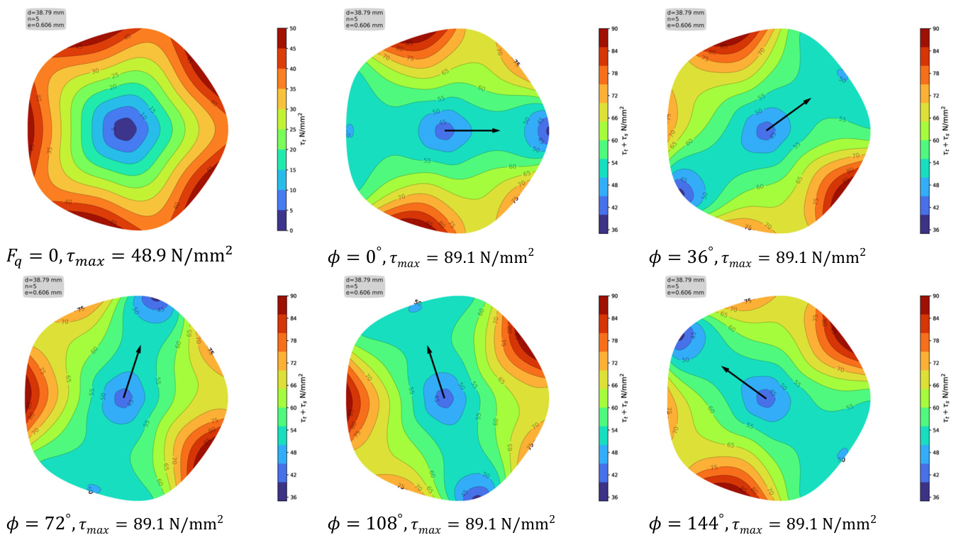
However, the effect of the rotating transverse force should not always be neglected. Figure 14 shows the distribution of the combined shear stress on the cross-section of a standard profile H5−40 × 37.58.
Figure 14.
Combined shear stress distribution on the cross-section of the H5−40 × 37.58 profile in various force angle positions for and Arrow: transverse shear force.
The figure clearly shows the effect of a rotating transverse force for different force angles .
Application to H-profile connections
This method of solution offers a reliable and cost-effective dimensioning of H-profiles. In many cases, a polygon connection fails outside the connection in a free shaft. However, since this is not known in advance, it is necessary to also check the basic shaft (without the hub). The analytical solutions from this work are useful and directly applicable here.
An evaluation based on standard profiles [5] shows that approximately 60% of the profiles have an eccentricity in the low-to-medium range and can be represented with good to very good approximation quality using the derived series coefficients and through (Equations (19)–(22)). For the remaining profiles, with higher eccentricity, the strategy described above can be extended as a prospect for future work by further increasing the series expansion, i.e., the number of leading terms retained. Since the resulting equations become correspondingly extensive in this case and are generally not favored by users in this form, an alternative for this range is to prepare the quantities of practical interest—for example, the maximum stresses—in tabular form for DIN 3689—Part 2, without having to state the underlying, extensive equations explicitly.
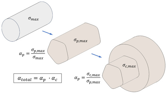
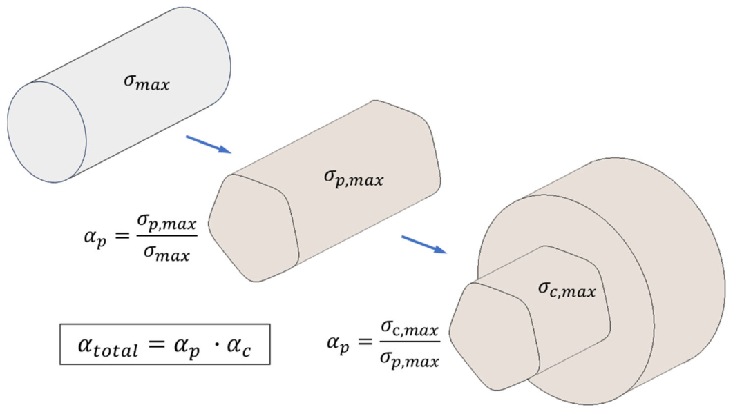
To test the connection area, a stress increase factor is used, which can be defined based on the corresponding stress in the free shaft. This is determined by comparing the analytically determined maximum stress with the corresponding maximum stress in a fictitious round bar with the nominal diameter of the H-profile . The ratio is referred to as the profile shape factor . The second shape factor, the connection factor , can be determined by the ratio between the stress in the connection and the maximum stress in the free shaft. Due to the different stress states in the connection, a suitable equivalent stress should be considered. It is not possible to determine this shape factor analytically; numerical and experimental methods can be used. This is currently the subject of an ongoing research project on H-profile connections [17]. The total stress factor is defined as the product of the two factors and enables the determination of a standard-compliant dimensioning rule, as shown in Figure 15.
Figure 15.
Concept for calculating a total form factor.
5. Conclusions
Building on [1,2,3], this work presented an analytical approach for determining shear stresses in non-circular profile cross-sections. The method was applied to hypotrochoidal profiles, so-called H-profiles, as defined in DIN 3689—Part 1, which in recent years have found increasing application in industry as shaft and shaft–hub connections.
Appropriate mapping functions for H-profiles were determined with good accuracy using a successive approximation method. These mapping functions enable the solution of both the transverse shear stress and the torsional stress. Solutions were derived for several examples from DIN 3689-Part 1 with different numbers of sides, showing excellent agreement with the corresponding numerical FE results. The formulation was further extended to cover the case of a rotating shear force.
Bending and torsional stresses were also addressed and calculated for selected examples. The combination of rotating shear force and stationary torsion was discussed as a particularly important load case, since the transverse shear stress then occurs as a stress amplitude and plays a significant role in the resulting stress state.
The results can be incorporated, in a suitable form, into DIN 3689—Part 2, “Calculation and Dimensioning.” They also provide a solid basis for extending the analysis to H-profile shaft–hub connections. In this context, two partial shape factors are relevant. The first, resulting from the profile contour, has been reliably determined in the present work. The second, resulting from the hub, will be addressed in future work. Together, these two contributions are intended to be incorporated into the standard.
Funding
This research received no external funding.
Institutional Review Board Statement
Not applicable.
Informed Consent Statement
Not applicable.
Data Availability Statement
The data presented in this study are available on request from the corresponding author.
Conflicts of Interest
The author declares no conflicts of interest.
Formula Symbols
| m-th Coefficient in the mapping function series | ||
| mm | Profile eccentricity | |
| - | Euler’s number | |
| MPa | Young’s modulus | |
| N | Shear force | |
| Coefficient functions in the mapping function series | ||
| Torsiol stress function in the polygon coordinate system | ||
| Bending stress function in the polygon coordinate system | ||
| Bending stress function in the Cartesian coordinate system | ||
| mm4 | Area moment of inertia in the Cartesian coordinate system | |
| Base circle | ||
| Rolling circle | ||
| mm | Length of profile shaft | |
| Nm | Bending moment | |
| Nm | Torsional moment | |
| - | Profile periodicity (number of sides) | |
| - | Number of terms in the mapping function series | |
| mm | Nominal or mean radius | |
| - | Profile parameter angle | |
| mm | Cartesian coordinates | |
| Complex function of polygon contour | ||
| Greek formula symbols: | ||
| - | Profile shape factor | |
| - | Connection shape factor | |
| - | Total stress factor | |
| - | Relative eccentricity | |
| Rotation angle of the coordinate system | ||
| Real stress function in Cartesian coordinate system | ||
| - | Physical plane unit circle | |
| - | Physical plane unit circle | |
| Poisson’s ratio | ||
| Real part of torsion function in polygon coordinates | ||
| Real part of shear function in polygon coordinates | ||
| Real part of shear function in Cartesian coordinates | ||
| Imaginary part of torsion function in polygon coordinates | ||
| Imaginary part of shear function in polygon coordinates | ||
| Imaginary part of shear stress function on the profile contour | ||
| Imaginary part of shear function in Cartesian coordinates | ||
| Curvilinear polygonal coordinates | ||
| MPa | Bending stress (z-component of stress vector) | |
| - | Polar angle | |
| MPa | Shear stress components | |
| MPa | Total shear stress | |
| MPa | Shear stress | |
| MPa | Torsional stress | |
| - | Coformal mapping function | |
| - | Complex variable in model plane | |
Appendix A. Mesh Convergence Study
To verify the mesh independence of the finite element results presented in Section 4, an additional mesh convergence study was carried out. Besides the mesh configuration used in the main analysis, two further discretizations were considered: a coarser mesh and a substantially refined mesh. Figure A1 summarizes the three mesh configurations along with their characteristic properties (e.g., element size, element type, number of elements/nodes).
Figure A1.
(a) Coarse, (b) reference, and (c) fine finite element mesh configurations considered in the mesh convergence study, with corresponding mesh properties, exemplarily carried out for a selected standardized profile.
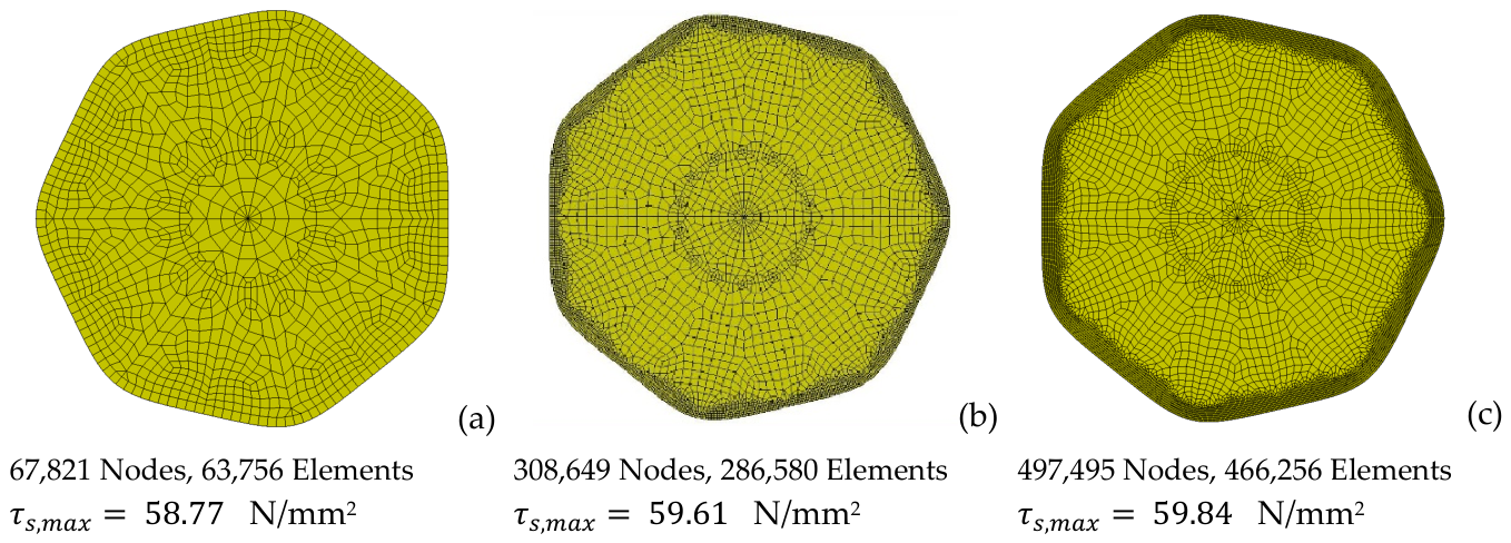
Figure A2 shows the resulting shear stress distributions obtained for all three mesh densities. The comparison shows only minimal differences between the results, with the mesh originally used in the manuscript and the finest mesh in particularly close agreement. This confirms that the mesh density adopted in the main analysis is sufficiently fine to yield mesh-independent results for the quantities of interest.
For completeness, it may be noted that the present finite element analysis is based on a linear-elastic material formulation, for which the solution is generally expected to be comparatively insensitive to mesh refinement, in contrast to nonlinear analyses, where results can depend much more strongly on mesh density.
Figure A2.
Shear stress distributions along the profile contour for the coarse, reference, and fine mesh, showing close agreement across all mesh densities, exemplarily carried out for a selected standardized profile.
References
- Muskelishvili, N.I. Some Basic Problems of the Mathematical Theory of Elasticity; Springer: Dordrecht, The Netherlands, 1977. [Google Scholar]
- Sokolnikoff, I.S. Mathematical Theory of Elasticity; Robert E. Krieger Publishing Company: Malaba, FL, USA, 1983. [Google Scholar]
- Ziaei, M. Shear and Bending Stresses in Prismatic, Non-Circular-Profile Shafts with Epitrochoidal Contours Under Shear Force Loading. Eng 2024, 5, 2752–2777. [Google Scholar] [CrossRef] [Scilit]
- DIN 32711-1:2009-03; Shaft to Collar Connection-Polygon Profil P3G—Part 1: Generalities and Geometry. Beuth-Verlag: Berlin, Germany, 2009.
- DIN 3689-1:2021-11; Shaft to Collar Connection-Hypotrochoidal H-Profiles—Part 1: Geometry and Dimensions. Beuth-Verlag: Berlin, Germany, 2021.
- Wunderlich, W. Ebene Kinematik; Bibliographisches Institut: Mannheim, Germany, 1968. [Google Scholar]
- Zwikker, C. The Advanced Geometry of Plane Curves and Their Applications; Dover Books on Advanced Mathematics; Courier Corporation: Chelmsford, MA, USA, 1963. [Google Scholar]
- Musyl, R. Die kinematische Entwicklung der Polygonkurve aus dem K-Profil. Wärmewirtschaft 1955, 10, 18–22. [Google Scholar]
- Ziaei, M. Torsionsspannungen in Prismatischen, Unrunden Profilwellen mit Trochoidischen Konturen. Forsch. Ingenieurwesen 2021, 85, 985–995. [Google Scholar] [CrossRef] [Scilit]
- Timoshenko, S.P.; Goodier, J.N. Theory of Elasticity; McGraw-Hill Book Company: New York, NY, USA, 1985. [Google Scholar]
- Kantorovich, L.V.; Krylov, V.I. Approximate Methods of Higher Analysis, Translation ed.; Dover Publications: Dover, UK; Mineola, NY, USA, 2018. [Google Scholar]
- Lee, K. Mechanical analysis of fibers with a hypotrochoidal cross section by means of conformal mapping function. Fibers Polym. 2010, 11, 638–641. [Google Scholar] [CrossRef] [Scilit]
- Ivanshin, P.N.; Shirokova, E.A. Approximate Conformal Mappings and Elasticity Theory. J. Complex Anal. 2016, 2016, 4367205. [Google Scholar] [CrossRef] [Scilit]
- Ziaei, M. Bending Stresses and Deformations in Prismatic Profiled Shafts with Noncircular Contours Based on Higher Hybrid Trochoids. Appl. Mech. 2022, 3, 1063–1079. [Google Scholar] [CrossRef] [Scilit]
- Ziaei, M. Bending and Torsional Stress Factors in Hypotrochoidal H-Profiled Shafts Standardised According to DIN 3689-1. Eng 2023, 4, 829–842. [Google Scholar] [CrossRef] [Scilit]
- MSC Software Corporation. Marc 2020 Manual; MSC Software Corporation: Newport Beach, CA, USA, 2020; Volume B (Element Library). [Google Scholar]
- Westsächsische Hochschule Zwickau; Technische Universität Chemnitz. FVA-Project 1031-1; Westsächsische Hochschule Zwickau: Zwickau, Deutschland; Technische Universität Chemnitz: Chemnitz, Germany, 2026. [Google Scholar]

Disclaimer/Publisher’s Note: The statements, opinions and data contained in all publications are solely those of the individual author(s) and contributor(s) and not of MDPI and/or the editor(s). MDPI and/or the editor(s) disclaim responsibility for any injury to people or property resulting from any ideas, methods, instructions or products referred to in the content. |
© 2026 by the author. Licensee MDPI, Basel, Switzerland. This article is an open access article distributed under the terms and conditions of the Creative Commons Attribution (CC BY) license.