


Abstract
Autonomous trading research pipelines can generate large volumes of machine-produced strategy proposals; however, testing them without leakage, overfitting, or silent selection bias remains an open problem. Existing autonomous trading systems primarily optimize strategy generation, whereas considerably less attention has been devoted to the governance of autonomous research pipelines that continuously generate, validate, and discard machine-generated hypotheses under strict temporal-integrity constraints. We introduce a season-structured validation and governance architecture that addresses this gap by combining leakage-free feature constraints, layered temporal validation, Bayesian risk-parameter optimization, and season-structured human oversight into a single reproducible workflow: within each season a local large language model (LLM) generates candidate strategies, and across season boundaries a human reviewer updates objectives and gates, forming a mixed-initiative governance layer. Across twelve adaptive seasons, 34,333 proposals produced 329 accepted strategies. Two case studies—a BNB/USDT candidate and a BTC/USDT replication—passed the predefined validation gates and showed positive selection-holdout performance under conservative calendar-time risk metrics. A feature-catalog sensitivity analysis on the BTC/USDT case study found that 3 of 50 random feature subsets of the same catalog reached the selected candidate’s recorded holdout Sharpe, with holdout Sharpe increasing with subset size and the comparison not budget-matched. A post hoc code audit conducted during the revision of this paper, disclosed here as an author-identified correction, found that the feature list included in every LLM proposal was never applied to training in any season: every reported model was trained on the full leakage-free catalog. As a result, this analysis compares the full catalog against random subsets, not LLM feature selection against chance. Therefore, the contribution is the validation and governance architecture itself, which turns a large stream of machine-generated proposals into a small set of credibly testable candidates, rather than any superior LLM feature intuition. Because the reviewer’s between-season adjustments consume out-of-sample information, the season sequence is a prolonged model-selection procedure. The case studies are therefore descriptive evidence of candidate rejection, not prospective proof of profitability.
1. Introduction
Algorithmic trading research is traditionally labor-intensive. A researcher hypothesizes a signal, writes code, engineers features, tunes parameters, and validates the result out-of-sample. Each step is susceptible to look-ahead bias, data snooping, and overfitting [1,2]. The proliferation of candidate factors has made multiple-testing corrections essential, because even random rules yield spuriously significant backtests at scale [3]. Recent advances in large language models (LLMs) have opened the possibility of automating parts of this pipeline—from code generation [4] to factor mining [5]—prompting dedicated surveys [6].
Most published frameworks rely on heavy human supervision or treat the LLM as a black-box oracle without explicit safeguards against leakage or overfitting [1,7,8]. Simultaneously, the emerging generation of autonomous quant-agent systems has focused on capability—richer agent architectures and verifiable task benchmarks [9,10]—while recent studies show a gap between simulated evaluation and deployable trading performance [8,11]. Existing autonomous trading systems primarily optimize strategy generation, whereas considerably less attention has been devoted to the governance of autonomous research pipelines that continuously generate, validate, and discard machine-generated hypotheses under strict temporal-integrity constraints.
The objective of this study is to propose and evaluate a season-structured, human-in-the-loop architecture in which an LLM agent autonomously proposes, codes, validates, and backtests directional cryptocurrency strategies, with leakage prevention and overfitting control as core design constraints. Trading is treated as a closed-loop analytics problem in which predictive modeling, simulation, and optimization prescribe actionable decisions subject to temporal-integrity and statistical constraints [12,13].
This study is guided by three research questions. RQ1: Does a season-structured, human-in-the-loop architecture, through leakage-free feature constraints and layered validation, constrain the risk of leakage and overfitting in autonomous strategy discovery? RQ2: What role do the governance mechanisms embedded at season transitions—acceptance gates and human review—play in the reliability of an autonomous LLM-driven research pipeline? RQ3: In the Season-12 case study, does the LLM’s proposal add value beyond that achieved by a constrained random search over the same leakage-free catalog? A post hoc code audit conducted during the revision of this paper (Section 4.8) found that the feature list of the LLM’s proposal schema was never applied to training in any season. RQ3 as originally posed also asked whether the LLM contributes feature-selection value; that component cannot be evaluated within Seasons 1–12, and Section 4.8 answers the executable version of the question—whether the accepted candidate’s full-catalog configuration outperforms random feature subsets drawn from the same catalog.
In this framework, an experimental season is the operational unit of a human-in-the-loop interaction cycle for quantitative investment, grounded in mixed-initiative governance principles [14,15] and generative curriculum learning [16]. Inside a season, the LLM agent autonomously operates under fixed constraints. At the season boundary, a human reviewer inspects the accepted candidates, updates the objective, tightens acceptance gates, and resets the scoring weights. Seasons are ordered as an exploratory curriculum, with looser early gates casting a wide net over the strategy space and later seasons applying stricter temporal-integrity and holdout criteria. Confining unbounded autonomous search to bounded, governed seasons makes leakage prevention and overfitting control enforceable as first-class architectural invariants.
The season mechanism differs from existing generation–feedback–regeneration loops in three specific ways. First, search proceeds in bounded batches under frozen gates, so every governance change is atomic and auditable at a season boundary rather than applied opportunistically mid-search. Second, the reviewer’s authority is restricted to objectives, gates, and scoring weights. The reviewer never approves or edits individual candidates, thereby separating strategic control from tactical execution. Third, the season sequence forms an explicit curriculum with a written transition rationale (Section Governance and Accountability; Supplementary Table S2). This contrasts with per-iteration human-in-the-loop designs such as Alpha-GPT [5], where a human refines each proposed factor, and with fully autonomous self-improving loops such as FinAgent [10], where no comparable boundary-level governance exists.
This study combines three elements. We integrate LLM-driven proposal generation, leakage-free feature constraints, layered validation, and an evolving composite score into a single autonomous research loop—a combination that is novel, to our knowledge, inside a season-structured, human-in-the-loop pipeline. The open-source implementation—a local 7B-parameter LLM, abstract syntax tree (AST)-based future-leak detection, and Numba-accelerated backtesting—makes thousands of autonomous iterations feasible on consumer hardware. Two candidates (BNB/USDT and BTC/USDT) passed the pipeline gates and showed positive selection-holdout performance under conservative calendar-time metrics (Section 4.2 and Section 4.3).
The LLM functions as a high-volume proposal generator, and not as a source of superior financial intuition. A post hoc code audit conducted during the revision found that the feature list included by the LLM in each proposal was never applied to training: every accepted model was trained on the full leakage-free catalog. A feature-catalog sensitivity analysis (Section 4.8) shows that random subsets of the catalog rarely match the full catalog—3 of 50 reach its recorded holdout Sharpe—although holdout Sharpe rises with subset size and the subsets received a smaller optimization budget. Therefore, the scientific contribution is the validation and governance architecture, which turns a large stream of machine-generated proposals into a small set of testable candidates.
The sequence of seasons constitutes an adaptive meta-search that gradually consumes out-of-sample information because the human reviewer updates season objectives, acceptance gates, and scoring weights after observing prior holdout results. Therefore, the reported selection-holdout results are evidence that the architecture can reject unsound candidates, not prospective proof that the surviving strategies possess a durable trading edge (Section 4.6 and Section 5.3).
2. Related Work
2.1. LLMs for Strategy and Factor Generation
The use of LLMs in quantitative finance has rapidly expanded, prompting dedicated surveys of the area [9]. Kou et al. [17] proposed a risk-aware multi-agent system that uses LLMs to generate alpha factors and dynamically weight them. Wang et al. [5] introduced Alpha-GPT, an interactive framework in which an LLM proposes factors that are refined by a human quant. Alpha-GPT 2.0 [18] moved toward self-evolving agents that discover alphas with limited human input. Zhang et al. [19] simulated stock trading with LLM-based agents in near-real-world environments. This line has since split into two. In factor mining, Yu et al. [20] generated synergistic formulaic alpha collections via reinforcement learning, while Zhang and Maringer [21] improved recurrent reinforcement learning for equity trading using a genetic algorithm. For multi-agent execution, Fang et al. [22] learned intention-aware communication for optimal multi-order execution. These studies show that, although LLMs can generate economically meaningful signals, they typically operate at the factor or sub-decision level and still require human judgment—or a separate learned controller—for execution logic, risk management, and hyper-parameter tuning.
Our work differs in scope: the LLM proposes the complete strategy—including entry rules, stop-loss, take-profit, probability threshold, and a feature set that is validated against the catalog but never consumed by training—and the system validates it end-to-end without human approval of individual candidates.
Chain-of-thought prompting [23] and the tight integration of reasoning with action in ReAct-style agents [24] are directly relevant to our pipeline. The LLM does not just emit a factor or a signal; it constructs a structured proposal, reflects on previous failures stored in the prompt, and generates executable code that is then validated by the environment. This positions the system between generative AI and autonomous experiment execution.
Factor mining with machine learning is a central topic in empirical asset pricing. Gu et al. [25] showed that machine-learning methods can forecast expected returns from large panels of characteristics, whereas Harvey et al. [3] documented how data mining heavily inflated the cross-section of published factors. Our pipeline combines both perspectives: it uses gradient-boosted classifiers to mine predictive features, but it constrains the search space with a leakage-free feature catalog and evaluates every candidate on a holdout set that is never used during optimization.
2.2. Automated Machine Learning for Trading
AutoML methods such as genetic programming [26,27], Bayesian optimization [28], and reinforcement learning [29] have long been used for trading strategy discovery. FinRL [11] provides a comprehensive reinforcement-learning framework for quantitative finance, while LLM-GA [30] combines genetic algorithms with LLM-generated seeds. Sun et al. [31] surveyed reinforcement-learning methods for quantitative trading. Recent reinforcement-learning work has shifted from raw predictive power to deployability: Detzel et al. [32] compared asset-pricing models after transaction costs, and DeepAries [33] learned when to rebalance rather than just what to hold. Although these approaches can search large strategy spaces, they often lack interpretability and require careful reward shaping to avoid overfitting.
General-purpose AutoML frameworks such as TPOT [34], AutoGluon [35], and Auto-sklearn [36] automate model selection and hyper-parameter tuning for tabular tasks. However, they are not designed for financial time series. They lack native temporal cross-validation, do not enforce embargo or purging between folds, and do not incorporate trading-specific constraints such as slippage, fees, or per-bar lookahead checks. Trading therefore requires an AutoML architecture in which leakage prevention and out-of-sample validation are first-class components rather than optional wrappers.
Our system uses Bayesian optimization (Optuna) only to determine the final risk-management parameters of a strategy. The LLM’s proposal schema includes a feature list, but a post hoc code audit conducted during the revision of this paper found that the training pipeline never consumed it: every model in every season was trained on the full leakage-free catalog, so no feature-design stage exists inside the pipeline and no feature search space exists for Optuna to inherit. What remains is a clean separation between proposal generation and parameter tuning, which keeps the optimization problem small and interpretable. Here, the staged search mirrors the automated machine-learning literature, where the model structure and hyper-parameters are optimized sequentially to maintain tractability [37].
2.3. Overfitting, Multiple Testing, and Statistical Rigor
Backtest overfitting is the main challenge in algorithmic research. Bailey and López de Prado [1] showed that the maximum Sharpe ratio observed after many independent trials is biased upward, and they proposed the deflated Sharpe ratio (DSR) to correct for selection bias and non-normality. Harvey and Liu [2] emphasized the importance of out-of-sample testing and multiple-testing adjustments in finance. Lo [38] discussed the statistical properties of the Sharpe ratios under non-independent and identically distributed (non-i.i.d.) returns. For dependent return series, block-bootstrap methods such as the stationary bootstrap [39] and the broader theory of resampling for dependent data [40] are preferred over naive i.i.d. resampling because they preserve serial dependence. Therefore, the bootstrap diagnostics reported here pair i.i.d. resampling with the stationary bootstrap as a dependence-preserving sensitivity check (Section 4.6). Beyond this foundational work, Jobson and Korkie [41] and Ledoit and Wolf [42] developed robust inference procedures for Sharpe ratios that remain valid under non-normality and dependence, while Romano and Wolf [43] provided stepwise multiple-testing corrections that control the family-wise error rate when many strategies are examined in sequence. Sullivan, Timmermann, and White [44,45] and White’s [46] reality check showed that apparently profitable trading rules often disappear once data-snooping is accounted for, and Hansen [47] developed a test for superior predictive ability that is directly applicable when a large panel of candidate strategies is screened. Harvey et al. [3] surveyed a cross-section of published factors and showed that most apparent anomalies are likely artifacts of data snooping. These concerns have acquired new urgency in the age of automated discovery: a recent post-mortem of a highly automated, self-evolving trading system documented the catastrophic divergence between validation and live performance [48]; recent work argues that statistical rigor must be enforced structurally within the discovery loop rather than checked afterward, supported by classical false-discovery-rate control [49]; and studies of LLM-based trading systems show that seemingly minor execution assumptions can render reported results irreproducible [50].
We put these insights into practice: every reported strategy is evaluated on a holdout set that was never used by Optuna, and we compute bootstrap p-values and an approximate multiple-testing-adjusted Sharpe ratio (inspired by the DSR construction) to estimate how likely the observed performance is to have arisen by chance. Following [49] and the reproducibility audit of [50], these safeguards are enforced inside the autonomous loop—through leakage-free feature constraints and layered temporal validation—rather than applied only to the final selected strategy.
2.4. Composite Scoring and Strategy Selection
Strategy selection in automated research requires more than maximizing a single in-sample metric. While standard quantitative workflows evaluate strategies across multiple, independently reported dimensions—including the Sharpe ratio, drawdown, win rate, and turnover—as distinct diagnostic statistics [51], automated discovery engines often combine these metrics into a single composite fitness function to guide heuristic search [26,30]. Recent work has proposed formal statistical adjustments to penalize selection bias and multiple-testing inflation, such as the haircut Sharpe Ratio [2] and the deflated Sharpe Ratio [1], as well as combinatorial validation frameworks to stress-test regime instability [16,51]. Yu et al. [20] evaluated formulaic alphas on several efficiency-aware axes rather than by return alone.
Our composite score combines the validation Sharpe, holdout Sharpe, holdout return, maximum drawdown, and a cross-validation area-under-the-curve (AUC) penalty. The score is reweighted across seasons based on observed failure modes, which creates a curriculum for the LLM agent.
2.5. Prescriptive Analytics and Autonomous Analytics Pipelines
Predictive analytics forecasts future outcomes from historical data, whereas prescriptive analytics recommends or automates decisions that optimize an objective under constraints [13,52]. Bertsimas and Kallus [12] formalized the shift from prediction to prescription, showing how machine-learning predictions can be combined with optimization to produce actionable policies. Separately, a strand of autonomous analytics pipelines has appeared in quantitative finance, in which agents iteratively propose, backtest, and refine strategies: FinAgent [10], for example, formalized a self-improving loop for quantitative investment. This has prompted the development of verifiable evaluation environments and closed-loop benchmarks for such agents [53,54], reflecting the growing recognition that autonomous quant systems must be judged on reproducible, cost-aware, out-of-sample protocols rather than single headline backtests.
Our contribution is an offline prescriptive-analytics research pipeline: it discovers, validates, and selects decision policies, but it does not trade live. Deploying a selected policy would require a separate online system that reads current market features and prescribes positions. We treat the offline research phase as prescriptive analytics because its output is a complete decision policy optimized end-to-end for a stated objective and validated on holdout data; however, we do not claim live deployment results. This aligns with the design-science view that a research artifact can be evaluated by its ability to produce well-validated prescriptions even before operational deployment [55]. Relative to the benchmark-driven agent literature [53,54], our emphasis is complementary: we do not focus on richer agents or broader task suites; instead, we focus on a season-structured governance layer that decides which autonomously generated candidates are trustworthy enough to retain.
2.6. Human-in-the-Loop Research and Mixed-Initiative Control
Fully autonomous research raises questions about control and interpretability. Horvitz [15] introduced the principles of mixed-initiative user interfaces, where humans and intelligent systems collaborate rather than work in isolation. Amershi et al. [14] turned these ideas into guidelines for human–AI interaction, noting that systems should communicate uncertainty, allow human override at appropriate moments, and improve from user feedback over time.
Our pipeline puts these principles into practice by confining full autonomy within a season and keeping human review for season transitions. The human reviewer updates the season objective, acceptance gates, and scoring weights based on the distribution of accepted strategies. This is a mixed-initiative design: the machine runs thousands of experiments and surfaces patterns, while the human steers the research direction and guards against objective drift. In this sense, the season boundary operationalizes mixed-initiative control: it gives the human reviewer explicit authority over objectives and acceptance criteria without requiring case-by-case approval of individual candidates. Table 1 summarizes how the systems discussed in this section compare along the dimensions most relevant to this work.
Table 1.
Comparison of autonomous and semi-autonomous trading research systems.
3. Methodology
3.1. System Overview
Definition 1
(Experimental season). An experimental season is the operational unit of a human-in-the-loop interaction cycle for quantitative investment: a bounded period of autonomous search during which the LLM agent operates under fixed constraints—a fixed objective, acceptance gates, scoring weights, and feature catalog—while all human intervention (inspection of accepted candidates, objective updates, gate adjustments, and score reweighting) is deferred to the season boundary, a review that typically takes 15–30 min per transition. The sequence of seasons implements a curriculum: earlier seasons use looser gates to explore the strategy space, and later seasons use stricter temporal-integrity and holdout criteria.
The autonomous research loop has five stages:
- Hypothesis generation: The LLM receives a prompt describing the current season’s goal, past failures, and the feature catalog, and proposes a strategy as a JSON object. The JSON schema includes a feature list, but a post hoc audit found that this list was never consumed downstream: training always used the full catalog (Section 4.8).
- Code generation: The LLM writes Python code implementing the strategy, including feature engineering, model training, and signal generation.
- Validation: A five-layer validator checks syntax, execution, AST-based future-leak detection, required-field presence, and feature-catalog compliance.
- Optimization: Optuna tunes stop-loss, take-profit, and probability threshold on the training/validation window.
- Evaluation: The strategy is simulated on the holdout window; if it passes the acceptance gates, it is recorded as accepted.
The loop repeats until a season budget is exhausted or a target number of accepted strategies is reached. Accepted strategies are ranked by a deploy score, and the best is selected as the production candidate. Figure 1 shows the overall architecture, and Figure 2 summarizes the season-level timeline: each season runs autonomously under fixed gates and objectives and ends in a human review that gates the transition to the next season, culminating in the final candidate selection.
Figure 1.
Autonomous strategy research architecture incorporating LLM-based proposal generation.
Figure 2.
Season timeline: each season runs as an autonomous loop under fixed acceptance gates and objectives; human review occurs only at season transitions, where gates and objectives are updated, and the sequence ends in the final candidate selection.
3.2. Feature Catalog and Temporal-Ordering Constraints
All features are computed from OHLCV data at 15-minute, 4-hour, and daily timeframes. The catalog includes technical indicators (RSI, MACD, Bollinger Bands, ADX, ATR, Stochastic RSI, and EMA differences), volatility measures, and lagged returns. Every feature is normalized by price or bounded to the current bar, and higher-timeframe indicators are merged into the 15-minute bars only after the corresponding candle has closed. The merge module shifts each higher-timeframe timestamp from its open time to its close time and then uses a backward-looking as-of merge; a daily value observed on day t therefore first becomes available to the 15-minute model at the close of day t. The validator parses the generated code into an AST and rejects any strategy that references absolute prices after the decision point or that accesses data outside the current bar. These precautions are consistent with standard defenses against leakage in data mining [7] and backtest overfitting [56], and with López de Prado’s [51] emphasis on purging and embargo in financial cross-validation: observations that overlap a test period due to long investment horizons, or strongly autocorrelated returns, must be excluded from training and from immediate post-test retraining. Our one-bar look-ahead lag for higher-timeframe merges and the AST-based price-reference check implement these principles in code. We treat this temporal-integrity layer as a design invariant; it is enforced in code review and verified by the out-of-sample stability reported in the results.
We additionally subjected the validator to a direct self-test rather than relying on code inspection alone. A battery of 18 deliberately invalid configurations was passed through the five-layer validation of Section 3.4: future returns via negative shifts, capitalized absolute-price columns, feature names implying future data, forward-shifted higher-timeframe references, direct future-price references, mutation of the feature list, missing mandatory parameters, inverted stop-loss ranges, and syntax or runtime errors. Fifteen of the 18 probes were correctly rejected, most by the sandbox-execution layer and the feature-catalog whitelist, with the AST price-reference check as backup. Three evasion vectors passed both the execution and AST layers: attribute access (df.close instead of df["close"]), dynamic column-name construction ("clo" + "close"), and getattr under a try/except guard; the AST rule visits only literal-string subscript nodes, and guarded execution suppresses the resulting errors. These bypasses cannot place a leaked column into the model, because FEATURES entries are validated against the catalog whitelist as literal strings and the pipeline reads only catalog features, so the evaded code can only execute dead code. We document this residual attack surface explicitly: the effective leakage control is the catalog whitelist, with the AST check serving as a first line of defense rather than a complete one.
3.3. Training and Backtesting Engine
Labels are generated with a barrier-based method adapted from the triple-barrier scheme of [51]: each trade carries a profit-taking barrier and a stop-loss barrier but no vertical time barrier, so positions close only when one of the two price barriers is touched and the holding horizon is empirical rather than fixed; positions still open at the end of the labeled window are dropped unlabeled. An XGBoost classifier [57] is trained on the training set, and predictions are converted into signals. The backtester simulates trades using Numba-accelerated code. Costs are modeled as a 0.20% round-trip fee plus 0.10% slippage on entry, following the transaction-cost framework used in optimal execution literature [58]. Stop-loss and take-profit exits are executed at the triggered level without additional slippage in the baseline configuration; Section 4.5 reports a stress-test that adds up to 1.00% symmetric slippage on all exits.
All Sharpe ratios reported by the engine and in the statistical audit are computed from daily equity changes and annualized with , the standard convention for cryptocurrency markets. This convention is used consistently across validation, holdout, and the secondary selection holdout periods.
An optional volatility kill-switch (atr_kill) zeros model probabilities when the 15-minute ATR exceeds a rolling multiple, preventing entries during extreme volatility spikes. The ATR and ADX indicators used for volatility and trend-strength filtering follow the original definitions of Wilder [59]. In the selected production candidate (S11 iter 1077), the kill-switch was configured at 3.0 rolling standard deviations. Candidate acceptance also requires a maximum drawdown below −15%.
3.3.1. Trading Chronology and Execution Assumptions
The simulation loop in pipeline/backtest.py::simulate_numba applies the following chronology, which we state explicitly because execution assumptions can materially change reported results [50]. All signals use only closed bars: 15-minute features are computed on the just-closed bar, and higher-timeframe values become available only after the corresponding candle has closed (Section 3.2). At each closed 15-minute bar, the model produces a probability for that bar; if the probability clears the acceptance threshold, the ADX value exceeds the configured floor, and fewer than the configured maximum number of positions are open (five in the reported S11 configuration, two in the S12 configuration), the engine enters at that bar’s close price plus 0.10% entry slippage. Position size is a fraction of an equal slot: capital is divided into that many equal slots, and the filled fraction scales linearly from 50% to 100% of one slot with the model’s confidence above the threshold. On each subsequent bar, open positions are checked against their barriers with the stop-loss evaluated before the take-profit, so when both levels are touched within the same bar, the stop-loss is assumed to execute first, a conservative ordering; stop-loss and take-profit exits fill at the triggered level with no additional slippage, and the 0.20% fee applied to exit proceeds models the round-trip cost. Positions still open at the end of a test window are closed at the final bar’s close. For equity accounting, open positions are carried at their entry cost rather than marked to market intra-trade, so the equity curve moves only when positions open or close. The mark-to-market recomputation in Section 4.3 reports how much this convention flatters drawdown. Daily equity changes are aggregated every 96 bars and annualized with .
Execution-timing sensitivity protocol. The entry price above is the close of the bar that produced the signal, so the reported results embed a decision price that becomes observable only once that bar has ended. Reporting standards for trade-relevant studies ask that signal formation and order timing be specified clearly enough to distinguish same-period from delayed execution [50]. We therefore specified a sensitivity grid over two axes and report it in Section 4.5. The first axis varies the fill across three prices. The close of the signal bar is the configuration used throughout this paper. The open of the following bar is the earliest price at which the decision could be acted upon. The close of the following bar imposes a full period of delay; it is the intraday analog of the one-period rule used in relative-value studies to neutralize bid-ask bounce [60]. The second axis varies the entry friction over three levels. The first two are the baseline 0.10% and 0.25%, the most severe friction setting used in the reproducibility audit cited above [50]. The third scales the baseline by the time-series dispersion of the spread, measured as the ratio between the 95th percentile and the median of the daily effective spread estimated over the same window with the estimator of Corwin and Schultz [61]. The estimator of Abdi and Ranaldo [62] was computed on the same windows, but it truncates 48–54% of the daily estimates at zero, which sets its median to zero in three of the four windows and leaves the ratio undefined; the Corwin–Schultz ratio is therefore used. The timing axis was fixed before any run; the friction levels replace a first specification that used the estimated spread levels directly (about 1.2–1.7% per side), for the reason given in the next sentence. We use both estimators for dispersion only, not for levels: applied to daily cryptocurrency data they return implausible spread levels for these venues, and they are reported to track the time-series variation of spreads well, while other estimators are preferable for levels [63]. Everything else is held fixed across the grid—the saved models, the risk parameters, the fee, the position limits, the evaluation windows, and the label set—and no component is re-optimized under any scenario.
To mitigate overfitting, we use a nested temporal split:
- Training: Oldest 60% of the in-sample window.
- Validation: Next 20%, used for early stopping and Optuna.
- Holdout: Most recent 20%, never seen by Optuna.
For Season 12, the split was extended to 2017–2020 training, 2021–2023 validation, and 2024–2025 holdout.
3.3.2. Walk-Forward Cross-Validation
Inside the training window, XGBoost hyper-parameter search and the reported cross-validation AUC use scikit-learn’s TimeSeriesSplit with three and five folds, respectively. Each fold is a contiguous block: fold t is trained on all observations up to a split point and tested on the immediately following block. This preserves temporal ordering but does not apply explicit purging or embargo between folds. Because the label generator has no vertical barrier (Section 3.3), a training-fold trade can in principle remain open after the next fold has begun, so we quantified this overlap directly for the two case-study configurations. The empirical holding horizon has a median of 2.4 days and a maximum of 29.2 days for the S11 iter 1077 configuration, and a median of 4.4 days and a maximum of 45.1 days for the S12 iter 5502 configuration. Under the five-fold TimeSeriesSplit, the number of training-fold events whose exit bar reaches or passes the first test-fold entry bar is at most two per fold (0–1.1% of the training labels) for S11 and at most four per fold (0.6–3.3%; the worst case is the first fold, which has the smallest training set) for S12. Rather than argue from materiality, we reran the five-fold cross-validation with those events removed. Three variants were compared: the procedure as run, a purged variant that drops every training event whose exit bar reaches the first test-fold entry bar, and a purged-plus-embargo variant that additionally drops training events entered within one median holding horizon of the boundary (227 bars for S11, 419 for S12). The purge removes five training events in total for S11 and eighteen for S12, reproducing the overlap counts above fold by fold; the embargo removes eight and thirty-eight. The mean cross-validation AUC moves from 0.572 to 0.563 (purged) and 0.563 (embargo) for S11, and from 0.537 to 0.535 (purged) and 0.542 (embargo) for S12. Every difference is well below the dispersion across folds: at most 0.009 against a standard deviation of 0.12 for S11, and at most 0.006 against 0.04 for S12, where the embargo variant moves the mean upward rather than downward. The reported cross-validation figures therefore do not depend on the absence of purging. These reruns use the representative-barrier label set of the overlap analysis, so their absolute AUC values differ slightly from the per-iteration figures logged during the seasons; the comparison of interest is between variants, which share that label set. We follow the purging-and-embargo principle [51] in reporting both variants, while recording that the pipeline as executed does not purge by construction. The final model is retrained on the full training window (the years between train_start and train_end, not the validation or holdout windows) after hyper-parameter selection via walk-forward cross-validation; the validation and holdout windows are never used for model fitting, only for evaluation and deployment scoring.
3.4. LLM Agent and Prompt Engineering
The LLM agent is a local Qwen2.5-7B-Instruct model served via llama.cpp. The choice of a 7B-parameter model is deliberate: it is small enough to run locally on consumer-grade GPUs via llama.cpp, which keeps the research loop private (no strategy code or market data is sent to external APIs) and eliminates per-token API costs across tens of thousands of iterations. Despite its size, the model generates syntactically valid Python strategy proposals in the constrained JSON schema used by the pipeline.
Across Season 11, the five-layer validation and scoring infrastructure rejected 94.4% of the 3797 candidates: 18.5% failed code validation (syntax, execution, AST future-leak, or feature-catalog compliance), 9.1% were duplicate parameter configurations, 18.8% converged to a previously discovered Optuna optimum, and 48.1% passed all code and optimization layers but failed the performance gates (AUC, validation Sharpe, holdout Sharpe, or drawdown). Only 5.6% were accepted. These rates indicate that the bottleneck is not the LLM’s proposal quality per se, but the multi-layer validation and scoring layers that filter out unsound candidates.
The prompt contains:
- The season objective (e.g., “improve holdout Sharpe on BTC”).
- A summary of the previous season’s accepted strategies and common failure modes.
- The feature catalog with exact function signatures.
- A JSON schema for the strategy proposal.
- Examples of valid and invalid code patterns.
The agent keeps a memory of recent failures to avoid repetitive proposals. Concretely, each new proposal prompt carries the season objective, the best result so far with its validation metrics, the top historical results, a summary of the last 30 iterations with their score, validation Sharpe, return, drawdown, AUC, and acceptance status, and up to five explicit rejection messages. The explicit rejection messages cover only failures detected before or during the pipeline run: code-validation errors, duplicate parameter configurations, and convergence to a previously discovered Optuna optimum. Holdout Sharpe values and the specific gate that failed are not transmitted to the LLM; however, because acceptance in Seasons 9–12 requires the holdout gate (Section 3.5), the accepted/rejected status visible in the iteration history is itself a channel through which holdout outcomes influence subsequent proposals. We therefore treat the holdout as a selection holdout rather than an independent final test (Section 3.5). After each season, a human-in-the-loop review updates the season objective and acceptance gates based on the distribution of accepted strategies. This is the primary point of human supervision; within a season, the loop runs without human approval of individual candidates. This mixed-initiative design follows the principles of Horvitz [15] and Amershi et al. [14]: the system performs the bulk of routine experimentation and surfaces structured results, while the human retains control over high-level goals and value alignment. The criteria used at each major transition are documented in Supplementary Table S2.
Governance and Accountability
Although the loop inside a season is autonomous, several mechanisms constrain the scope of autonomous decisions and allocate accountability.
Prompt and schema constraints. The LLM cannot propose arbitrary code. It must emit a JSON object with fixed fields (features, entry_logic, sl_pct, tp_pct, threshold, adx_min, atr_kill_threshold, and xgb_params) and use only functions from the leakage-free feature catalog. The prompt includes the season objective, a summary of the last 10–20 rejected proposals, and three in-context examples of valid and invalid code patterns. The temperature is initialized at 0.7 and annealed downward when the acceptance rate stalls, reducing exploration once the search has found a productive region.
Definition 2
(Season transition). A season transition is the human-governed boundary between two consecutive seasons, at which the season-transition review protocol is applied. At each transition, the human reviewer inspects: (i) the distribution of accepted strategies by AUC, Sharpe, and drawdown; (ii) the most common rejection reasons; (iii) the feature-importance patterns of accepted models; and (iv) any evidence of objective drift (e.g., falling validation Sharpe despite rising holdout Sharpe). Based on this, the reviewer updates the season objective, adjusts one or two acceptance bounds, and reweights the composite score. The reviewer records the rationale in season_notes.md, which becomes part of the audit trail.
Table 2 summarizes the major transitions; Supplementary Table S2 gives the full record.
Table 2.
Major season transitions: observed evidence, decision, and rationale.
Accountability allocation. We adopt a simple RACI-style model for the offline research phase:
- Responsible (autonomous agent): Proposing candidates, running backtests, and logging results.
- Accountable (human researcher): Setting season objectives, acceptance gates, and scoring weights; interpreting results; and deciding whether a candidate is promoted to further study.
- Consulted (code validator, statistical audit): Enforcing hard constraints and flagging suspicious patterns.
- Informed (future deployment system): Receiving the selected candidate and parameters, but not involved in research decisions.
This model applies to the offline research pipeline only. A subsequent live system would require a separate governance layer with real-time monitoring, circuit breakers, and compliance sign-off that are outside the scope of this paper. This operational structure instantiates, at the level of daily practice, the mixed-initiative governance principles [14,15] and the design-science view of a validated research artifact [55] introduced in Section 1.
3.5. Acceptance Gates and Composite Score
Definition 3
(Acceptance gate). An acceptance gate is a configurable, season-specific threshold that a candidate strategy must satisfy to be recorded as accepted. A strategy is accepted only if it satisfies all of the following configurable gates, which change across seasons:
- Cross-validation AUC above a season-specific threshold (typically ≥0.52–0.55).
- Sharpe ratio on the validation window above a season-specific threshold (typically ≥0.5–1.0).
- Sharpe ratio on the selection-holdout window above a season-specific threshold (typically ≥0.0–0.5).
- Maximum drawdown within the backtest objective bounds (the objective function rejects configurations with excessive drawdown).
- A minimum number of trades in the validation window.
- All code-validation layers passed.
Strategies are ranked by a composite score that combines the validation Sharpe ratio, the selection-holdout Sharpe ratio, the holdout return, the maximum drawdown, and a cross-validation AUC penalty. Formally, the ranking objective can be written as
where the weights were adjusted across seasons. The AUC term penalizes only below-chance discriminative ability; it does not penalize AUC values above 0.5, because higher validation AUC is desirable once the leakage checks have passed. The composite score is computed for every evaluated candidate, including those near the acceptance gates, and ranks pre-acceptance candidates for inspection; the AUC term is a guard against below-chance cross-validation AUC surviving the weaker gates of early seasons. Under the S9–S12 gate configuration (AUC ≥ 0.51–0.55), the term is inactive by construction, because any candidate that reaches the ranking stage already exceeds 0.5. In Seasons 9–12, the weights emphasized holdout Sharpe and drawdown control; strategies with negative holdout Sharpe or validation-holdout decay were heavily penalized. Inside the Bayesian optimizer, the objective function changed from maximizing the minimum validation Sharpe across sub-windows (score mode) to maximizing the average holdout return (profit mode), with hard constraints on drawdown and trade count.
We refer to the holdout window as a selection holdout rather than a passive or final test set. The selection holdout is never used by Optuna for parameter tuning, but it does participate in acceptance (the triple gate includes a holdout-Sharpe bound), in ranking (the composite and deploy scores include holdout terms), and in governance feedback (the season-transition reviewer observes holdout results before updating gates and weights). Consequently, no period within Seasons 1–12 remained fully untouched by the selection process: there is no fully independent final test set in this study, and the holdout results should be read as the output of a disciplined but adaptive selection procedure.
3.6. Deployment Score and Model Selection
For deployment selection, we use a deploy score that averages the selection-holdout Sharpe and the Sharpe on the secondary selection holdout (January–March 2026 for S11):
Because the deploy score includes , the 2026 period works as a secondary selection holdout: it was used to choose the production candidate from the 30 top holdout candidates that were re-evaluated for deployment from Season 11. It is therefore not an independent prospective test and should be treated only as a noisy post-selection observation. The selected candidate, S11 iter 1077, maximized this deploy score; the score is driven primarily by the selection-holdout Sharpe because the 2026 window contains only four trades and its Sharpe is extremely noisy.
The selected candidate’s selection-holdout Sharpe (2.58) comes from a population of 212 accepted strategies in Season 11, so it is also subject to selection bias. Under the simplifying assumption that the 212 accepted holdout Sharpes are i.i.d. normal with the observed mean (1.37) and standard deviation (0.61), the expected maximum among 212 draws is approximately 3.06 (95% interval: 2.66–3.62), and the observed maximum holdout Sharpe in that population (2.95, with the selected candidate at 2.58) lies within the range expected from pure selection; however, the positive mean of the accepted strategies (1.37) indicates that the accepted population as a whole has positive holdout performance. This selection-bias calculation follows the extreme value theory (EVT) framework developed by [1] to estimate performance inflation under multiple testing.
The Q1 2026 Sharpe is based on only four trades and is consequently very noisy; it should not be interpreted as precise evidence of live edge, nor used to rank the candidate against other candidates. We report it as a preliminary post-selection observation rather than as an independent out-of-sample result.
The case-study selection rule is therefore explicit. The S11 production candidate (iter 1077) is the candidate with the highest deploy score among the 30 top-holdout candidates re-evaluated for deployment. The S12 candidate (iter 5502) is the candidate retained at the Season-12 closure review as the best balance of validation Sharpe, holdout Sharpe, and out-of-sample equity. A third iteration, S11 iter 1066, appears only in the statistical audit (Section 4.6) as the accepted S11 candidate with the strongest bootstrap evidence; it was not a deployment candidate.
3.7. Experimental Configuration and Computational Budget
Table 3 summarizes the two strategies analyzed in detail. Table 4 reports how the search evolved across seasons. The full feature catalog is provided in Supplementary Table S1, and the inter-season design decisions are documented in Supplementary Table S2.
Table 3.
Case-study strategies.
Table 4.
Evolution of acceptance rate and best holdout Sharpe by season.
The experiments were run on a local workstation with a consumer GPU serving the Qwen2.5-7B-Instruct model via llama.cpp. Neither per-iteration wall-clock time nor energy use was logged, so the following figures are retrospective estimates: the full study (34,333 iterations across twelve seasons) required about 6–8 weeks of continuous execution, including restarts after memory-related crashes in early seasons, and LLM inference and Optuna optimization together consumed roughly 500–800 kWh. Per-iteration latency varied from seconds (for strategies rejected at the code-validation layer) to several minutes (for strategies that ran the full Optuna loop).
3.8. Reproducibility Protocol
To enable independent replication, we fixed the software environment, random seeds, data sources, and execution flow described below. All code, experiment logs, and generated artifacts are available in the repository associated with this submission.
Persistent archive. All code, experiment logs, and generated artifacts are publicly available at https://github.com/pesobreiro/algo-autoresearch-paper (accessed on 23 September 2026) (MIT license) and are permanently archived at Zenodo (DOI: https://doi.org/10.5281/zenodo.21160587).
Software environment. The pipeline was executed under Python 3.10.19 (conda environment ml_trading) with the following core package versions: pandas 2.3.3, NumPy 2.2.6, XGBoost 3.1.2, scikit-learn 1.7.2, Optuna 4.6.0, Joblib 1.5.3, PyArrow 22.0.0, and llama.cpp serving Qwen2.5-7B-Instruct (quantized GGUF, Q4_K_M). The multi-timeframe feature-merge module is imported from features.technical (commit hash recorded in requirements.txt). The full dependency list is in requirements.txt. We recommend creating a dedicated virtual environment and installing the pinned versions; newer versions may alter random number generation or sampler behavior and are not guaranteed to reproduce the exact numeric results reported here. One dependency deserves emphasis: the reported models were trained and serialized under XGBoost 3.1.2, and the holdout Sharpe ratios and the statistical audit of Section 4.6 reproduce exactly only when the saved models are loaded under that version. Under XGBoost 3.0.2, the predicted probabilities of the saved classifiers shift by up to (correlation ), which moves the S12 combined-period holdout Sharpe from 1.13 to 0.43; pinning the XGBoost version is therefore mandatory for exact reproduction, not merely recommended. (NumPy and Numba were upgraded after the experimental seasons concluded; the Numba-jitted backtest path is sensitive to this pairing, so exact reproduction of trade simulation should use the versions above.)
Random seeds. Determinism was enforced at three points: (i) the XGBoost classifier uses random_state = 42; (ii) Optuna’s TPE sampler is initialized with seed = 42 and n_startup_trials = 20 for the SL/TP/threshold study (and n_startup_trials = max(5, n_trials//4) when XGBoost hyper-parameters are also tuned); (iii) scikit-learn’s TimeSeriesSplit is used for walk-forward cross-validation. Because some operations rely on Numba JIT compilation and BLAS threading, byte-identical reproduction across operating systems is not guaranteed; however, the statistical conclusions are robust to the residual non-determinism.
Hardware. The main experiments ran on a Linux workstation with an NVIDIA GeForce RTX 2060 (6 GB) and an x86_64 CPU. The LLM server (llama-server) offloaded 32 layers to the GPU; the remaining CPU layers introduced per-token latency but no change to the generated distribution beyond temperature effects. CPU-only execution is possible but substantially slower.
Data. OHLCV bars at 15-minute, 4-hour, and daily resolutions were downloaded from the Binance public API and stored as Parquet files in a dedicated data directory (~/crypto_data). The raw data are publicly available; the ticker mappings are bnb_15m_usdt_binance, bnb_4h_usdt_binance, and bnb_1d_usdt_binance for BNB/USDT and btc_15m_ usdt_binance, etc., for BTC/USDT. We used the closing prices from the daily series to compute the buy-and-hold benchmarks. A download_data.py helper script in the repository performs the exact Binance API calls used in this study and records the date ranges of each file.
Repository structure. The repository contains:
- autoresearch/—LLM client, validator, tracker, and runner.
- pipeline/—label generation, XGBoost training, Optuna backtest, feature catalog, and research_params.py (the single file the LLM is allowed to rewrite each iteration).
- experiments_s{season}/—one JSON file per iteration with metrics, parameters, and status.
- best_models/season_{season}/—accepted model artifacts.
- deployment/—scripts to re-run the selected case studies and produce annual performance tables and benchmark comparisons.
Execution flow. A single season is launched with python main.py after copying config.yaml.example to config.yaml and starting the local LLM server. The runner executes the loop described in Section 3.1: proposal, validation, training, Optuna optimization, and holdout evaluation. The configuration file specifies the ticker, exchange, data directory, season identifier, and acceptance minima. The exact feature sets, indicator parameters, SL/TP/threshold ranges, and XGBoost hyper-parameters are written by the LLM into pipeline/research_params.py each iteration, with one exception: the FEATURES field, although rewritten each iteration, was never read by the training pipeline, so every reported model was trained on the full feature catalog (Section 4.8). For post hoc verification, the deployment scripts deployment/evaluate_models.py and deployment/backtest_deploy.py replay the selected iterations using the saved model and parameters, without calling the LLM.
Reproduction checklist. To replicate the two case studies reported in Section 4: (1) install the pinned environment; (2) download the Binance OHLCV data for BNB/USDT and BTC/USDT at the three timeframes; (3) start the LLM server with the Qwen2.5-7B-Instruct GGUF model; (4) run python main.py with the appropriate season number; (5) for the selected iterations, run the deployment scripts with the parameters recorded in best_models/season_{N}/iter_{XXXX}/meta.json. Because the search is expensive, a partial reproduction can focus on rerunning the saved case studies, which is computationally cheap and fully deterministic given the saved model and parameters.
4. Results
4.1. Search Convergence Across Experimental Seasons
Having characterized the population of 329 accepted strategies drawn from 34,333 proposals across twelve seasons (Table 4), of which the 313 strategies accepted in the four triple-gate seasons (S9–S12) record a comparable selection-holdout Sharpe with mean 1.09 and standard deviation 0.68 (median 0.92; overall acceptance rate 0.96%), we now examine in detail the two strategies retained as final candidates.
Figure 3 shows the acceptance rate and the best holdout Sharpe ratio per season. Season 1 was the manual initialization baseline (32 iterations, score 0.5607, no formal acceptance gates); the automated loop started in Season 2. The early automated seasons (S2–S4) produced no accepted strategies because the acceptance gates were too loose or the search space too unconstrained. Season 5 introduced a profit-mode objective and achieved the first acceptances (0.70%). Season 6 introduced stricter criteria, dropping the acceptance rate to 0.01% (1 in 12,864). Seasons 9–11 improve steadily in holdout Sharpe, co-occurring with three protocol changes: the selection holdout (S9), bear-market validation (S10), and the triple-gate protocol (S11); these changes co-vary with asset, time windows, and the proposal distribution, so the improvement cannot be attributed to any one of them (Section 5.3). Season 12 extended the training window back to 2017 and switched to BTC, a test of cross-crypto replication.
Figure 3.
Search convergence across experimental seasons (acceptance rate and best holdout Sharpe).
The acceptance rate reached its peak of 5.58% in Season 11, but this reflects a richer proposal distribution, not weaker gates: the average composite score fell from 2.03 in S9 to 1.09 in S11 because the scoring weights were renormalized when the acceptance gates tightened (S9 allowed only five strategies with high validation Sharpe but negative average holdout Sharpe; S11 demanded positive holdout Sharpe and lower drawdown, which compressed the score scale). The best holdout Sharpe rose from 1.00 to 2.95 over the same period, so quality improved even as the raw score range shifted.
Two properties of this search history matter for interpretation. First, Seasons S1–S8 are exploratory development seasons: the objective mode (score vs. profit), the acceptance gates, and the scoring scale were all still changing, and the S5–S7 scores are not comparable to the S9–S12 scale (Table 4). Seasons S9–S12 are the stabilized triple-gate protocol and carry the evaluation weight of this study. Second, the number of seasons was not pre-registered. The search ended after Season 12 because the cross-asset replication on BTC/USDT produced an accepted candidate, and the human reviewer closed the search; the stopping decision was therefore performance-contingent, which adds a study-level selection bias on top of the within-season selection (Section 5.3).
Table 5 generalizes the Season-11 breakdown of Section 3.4 to all four triple-gate seasons, decomposing each season’s iterations by the layer at which they were stopped. Two patterns recur. First, the dominant rejection layer in every season is the performance-gate failure of otherwise valid, non-duplicate candidates. Second, in Season 12, the duplicate-detection layers (identical parameter configurations and convergence to a previously discovered Optuna optimum) together discard 4212 proposals, indicating that the proposal distribution had converged onto a limited region of the search space. These architecture-level filtering statistics, rather than the performance of any single accepted strategy, are the primary evidence for the validation design.
Table 5.
Per-season filtering by validation layer, Seasons 9–12.
Acceptance decisions are also reasonably stable to small changes in the gates. Re-scoring every logged iteration that reached gate evaluation under 125 combinations of gate offsets (AUC , validation Sharpe , holdout Sharpe ) yields accepted counts between 106 and 484 for Season 11 (actual: 212, reproduced exactly at zero offset) and between 5 and 145 for Season 12 (actual: 93). The Season-12 accepted set is sensitive to joint tightening of both Sharpe gates—raising both by 0.10 leaves single-digit acceptances—but stable to small single-gate moves (roughly 75–115 under offsets). Acceptance counts therefore depend materially on the gate configuration; Section 5.1 returns to this dependence when interpreting RQ2.
4.2. Production Model Performance
The selected production candidate, S11 iter 1077, traded BNB/USDT over 2022–2025 (validation 2022–2024, selection holdout 2025); the January–March 2026 window was used only for deployment selection and is reported as a post-selection observation. Iter 1077 was selected by the deploy-score rule of Section 3.6. Figure 4 shows the equity curve. Table 6 gives the annual performance. The candidate produced positive returns in every year of 2022–2025 on the validation and selection-holdout windows. The maximum drawdown of realized equity during the validation period was −8.89%, well below the −15% gate.
Figure 4.
Equity curve—S11 BNB/USDT iter 1077 (2022–2026). The curve spans training (2022–2023), validation (2022–2024), the selection-holdout year (2025), and a post-selection observation window (Q1 2026, four trades); see Table 3 for exact period boundaries.
Table 6.
Annual performance of the selected production candidate (S11 iter 1077, BNB/USDT).
The strategy’s AUC of 0.5721 shows only marginal predictive power at the individual-bar level; the economic value comes from combining a calibrated probability threshold, asymmetric risk management (7.85% stop-loss vs. 7.07% take-profit), and an ADX regime filter [59] that avoids weak-trend entries. The wider stop-loss relative to take-profit came from Optuna optimization under the bear-market validation introduced in Season 10: it gives profitable trades room to survive short-term reversals while the high-probability threshold and ADX filter keep entry quality high enough that smaller, more frequent gains offset occasional larger losses.
This holdout Sharpe is drawn from a population of 212 strategies accepted in Season 11; Section 3.6 shows via an Extreme Value Theory analysis that the observed value (2.58, against a population maximum of 2.95) falls within the range expected from pure selection, while the accepted population as a whole has positive holdout performance (mean Sharpe 1.37).
Benchmark comparison. Table 7 compares the strategy’s annual returns with those of a passive buy-and-hold investment in BNB/USDT.
Table 7.
Benchmark comparison: S11 iter 1077 vs. BNB/USDT buy-and-hold.
4.3. Cross-Crypto Replication
To test whether the design transfers to a different cryptocurrency, we ran Season 12 on BTC/USDT with a training window starting in 2017. The selected candidate, S12 iter 5502, passed the validation gates and showed a validation Sharpe of 1.39 and an annual-average holdout Sharpe of 1.15, with a 27.7% compounded holdout return (2024–2025) and a maximum drawdown of realized equity of −8.13% on the validation period (Figure 5). Table 8 breaks down the annual performance. Returns are positive in every year; the weakest years were 2025 (+10.69%, a mildly negative year for the BTC benchmark) and 2021 (+10.91%, a late-bull period). The lower holdout Sharpe relative to S11 reflects Bitcoin’s different volatility regime, but the candidate remained profitable and within risk limits.
Figure 5.
Equity curve—S12 BTC/USDT iter 5502 (2021–2025).
Table 8.
Annual performance of the cross-crypto replication (S12 iter 5502, BTC/USDT).
Benchmark comparison. Table 9 compares the S12 strategy’s annual returns with those of a passive buy-and-hold investment in BTC/USDT. As with the S11 case, the strategy underperforms buy-and-hold in strong bull years (2021, 2023, 2024) but avoids most of the 2022 bear-market loss and produced positive returns in 2022 and 2025 when the benchmark was negative.
Table 9.
Benchmark comparison: S12 iter 5502 vs. BTC/USDT buy-and-hold.
The lower holdout Sharpe relative to S11 reflects Bitcoin’s different volatility regime, but the candidate remained profitable and within risk limits. This indicates that a research system incorporating an LLM agent can adapt its entry logic and risk parameters to a different asset while preserving temporal integrity; feature selection plays no role in this transfer, since all models in all seasons were trained on the same full catalog (Section 4.8).
Table 10 extends the benchmark comparison to risk-adjusted terms over the selection-holdout windows, using the engine and conventions of Section 4.6. The strategies’ annualized volatility is four to seven times lower than the benchmark’s, and their Sortino ratios are correspondingly higher (6.47 vs. 0.93 for S11; 2.12 vs. 1.45 for S12). The Calmar comparison is asymmetric: S11 clearly dominates (5.65 vs. 0.60), while S12 edges out buy-and-hold (1.34 vs. 1.25) despite the benchmark capturing most of the 2024 bull market. On realized equity, part of the drawdown control is therefore genuine risk-adjusted improvement (the mark-to-market values follow below), and part reflects lower market exposure: the strategies hold at least one open position on only 18.3% (S11) and 48.6% (S12) of bars. Normalized by exposure, S11 extracts a 104% return per unit of time in market, 4.7 times the benchmark’s 22%, while S12 extracts less than buy-and-hold per unit of exposure (61.2% vs. 96.3%)—its edge lies in the timing and selectivity of risk-taking rather than in a higher raw return rate.
Table 10.
Risk-adjusted comparison with buy-and-hold over the selection-holdout windows.
Mark-to-market valuation of the risk metrics. The engine carries open positions at their entry cost (Section 3.3.1), so the equity curve moves only when a position opens or closes and unrealized gains and losses are invisible while a trade is running. Because holding periods extend for weeks, we recomputed every metric in Table 10 from a mark-to-market equity curve, valuing each open position at the current bar’s close, with no other change to the models, parameters, or windows. The direction is uniform, and the magnitude is moderate. For S11 iter 1077, the holdout Sharpe falls from 2.58 to 2.48, the maximum drawdown deepens from −3.4% to −3.7%, the Calmar ratio falls from 5.65 to 5.14, and the total return is unchanged at 19.1%. For S12 iter 5502, the Sharpe falls from 1.13 to 1.01, the annualized volatility rises from 12.1% to 13.0%, the maximum drawdown deepens from −10.4% to −13.8%, and the Calmar ratio falls from 1.34 to 0.95. The total return falls from 29.7% to 27.8% because the window ends with an open position worth less than its entry cost. S11 remains above the benchmark on every risk-adjusted measure. S12 remains above it on Sharpe (1.01 vs. 0.95) and Sortino (1.59 vs. 1.45), but its Calmar advantage over buy-and-hold in Table 10 (1.34 vs. 1.25) reverses under mark-to-market valuation (0.95). The entry-cost convention flatters both drawdown and Calmar: the reported drawdown is a lower bound on the risk actually run, and the reported Calmar ratio is an upper bound on the risk-adjusted return.
The post-submission window makes the point sharply. Under the entry-cost convention, the S12 evaluation reports a maximum drawdown of 0.00%, which is an artifact: the six trades of that window closed at a profit and no loss was ever booked, so the curve never declined. Valued mark to market, the same window has a maximum drawdown of −2.1% and an annualized volatility of 7.2%. The drawdown-control claims of this paper should therefore be read as claims about realized equity under a barrier-exit strategy, not about the intra-trade path of the portfolio.
4.4. Feature Importance and Parameter Sensitivity
Figure 6 shows the top features for S12 iter 5502. Stochastic RSI and ADX at the daily and 15-minute timeframes dominate, followed by EMA differences and Bollinger Band width. The multi-timeframe pattern matches the findings of [8] for Bitcoin prediction: short-term momentum and medium-term trend strength carry complementary information. Reference [8] is by the same first author and shares the OHLCV data source and multi-timeframe feature-engineering approach; we cite it because it documents the same empirical regularity, not as independent validation.
Figure 6.
Top features—S12 iter 5502.
Optuna parameter importance (Figure 7) shows that the probability threshold explains 82–88% of the optimization variance across seasons, while stop-loss and take-profit contribute the remainder. This means that trade selection precision matters more than exact exit levels, once the exit range is broadly correct.
Figure 7.
Optuna parameter importance—S12 iter 5502.
4.5. Robustness to Transaction Costs and Market Regime
Figure 8 shows the sensitivity of S12 iter 5502 to additional exit slippage. Even with 1.0% of extra slippage on every exit, the final equity remains well above the break-even line, so the strategy’s edge is not an artifact of optimistic exit-cost assumptions. Entry costs are a different matter: S12 is considerably more sensitive to entry friction than to exit slippage (Table 11).
Figure 8.
Cost sensitivity of S12 iter 5502 (BTC/USDT) to additional symmetric slippage on all exits, above the baseline 0.20% fee and 0.10% entry slippage. Final equity is computed with the canonical pipeline engine (pipeline/backtest.py::simulate_numba) from an initial capital of EUR 500 over the 2024–2025 selection-holdout window; equity compounds chronologically within each calendar year, annual figures are computed independently, and the total return compounds the annual figures, following the accounting convention of Table 3.
Table 11.
Execution-realism sensitivity: selection-holdout windows under three entry-timing rules and three entry-friction levels.
Exit-slippage stress-test. We reran the exit-slippage sensitivity analysis under the canonical pipeline engine (pipeline/backtest.py::simulate_numba), the code that produced the meta.json metrics of Table 3. The rerun applies additional symmetric slippage on stop-loss, take-profit, and end-of-window exits and keeps the baseline 0.10% entry slippage and 0.20% round-trip fee. It follows the chronology and accounting conventions of Section 3.3.1: entry at the signal-bar close, stop-loss evaluated before take-profit within the same bar, adx_min = 0, the EUR-500 accounting compounded across the holdout years, and the holdout Sharpe computed as the mean of the per-year Sharpes. With zero extra exit slippage, the rerun reproduces the headline numbers exactly—S11: +19.10%, Sharpe 2.58, final equity EUR 595.52; S12: +27.67%, Sharpe 1.15, EUR 638.33—which resolves the engine discrepancy reported in the first submission: the earlier deployment-engine figures used different accounting conventions and are superseded. Over a grid of 0.05–1.00% additional exit slippage, degradation is monotone and approximately linear in both case studies (approximately 0.30 Sharpe points per 1.00% of exit slippage), and both strategies remain profitable across the whole grid. At 0.30% extra exit slippage, S11 returns +17.77% (Sharpe 2.49) and S12 +24.41% (Sharpe 1.07); even at a punitive 1.00%, S11 returns +14.71% (Sharpe 2.26) and S12 +17.12% (Sharpe 0.86). The S11 case is structurally more robust because its wide stop-loss (7.85%) and take-profit (7.07%) levels make small exit slippages a modest fraction of the expected trade return; the S12 case degrades faster in relative terms (a 25% Sharpe reduction at 1.00%, against 12% for S11), albeit from a lower base.
Execution-timing and entry-friction sensitivity. Table 11 reports the grid specified in Section 3.3.1, applied to the selection-holdout windows of both case studies. Filling at the open of the bar that follows the signal instead of at the signal bar’s own close leaves every reported figure unchanged (E1 versus E2 and E4 versus E5). The reason is mechanical: on a continuously traded venue, the two prices almost coincide. Across the bars on which a position was actually opened, the gap between the next bar’s open and the signal bar’s close had a median of 0.000% for both candidates and was exactly zero on 55% (S11) and 57% (S12) of those bars. Its maximum was 0.011% (S11) and 0.00002% (S12), one and four orders of magnitude, respectively, below the 0.10% entry slippage already charged. Imposing a full bar of delay (E3) costs 0.12 Sharpe for S11 and 0.02 for S12 (0.024 before rounding; see the note to Table 11), and leaves the post-submission evaluation of S12 unchanged (11.21% against 11.30%, identical Sharpe and trade count). The timing assumption is therefore not what carries the reported results.
The entry-friction axis separates the two candidates. S11 iter 1077 is insensitive to it: at 0.46% entry friction, more than four times the baseline, its holdout Sharpe moves from 2.58 to 2.46. S12 iter 5502 is not: at 0.25% its holdout return falls from 27.67% to 7.68% and its Sharpe from 1.15 to 0.37, and at 0.57% the return is 1.77%. Entry friction acts on this engine through the barrier band rather than as a direct charge. The stop-loss and take-profit levels are set relative to the fill price, so a worse fill moves the whole band upward and brings the stop closer to the prevailing price. That is why the effect exceeds the friction itself, and why the S11 return is not monotone in it, a path effect over 38 trades. This is a different channel from the exit-slippage stress-test above, where the same S12 configuration stayed well above break-even: the S12 edge is robust to what is paid on exit and fragile to what is paid on entry. The post-submission window of S12 is unaffected across the grid (11.21% to 10.89%), but it contains only six trades and cannot settle the question.
Figure 9 reports mean trade return by ADX regime. The strategy performs best in trending markets (ADX 20–40) and strong-trend markets (ADX > 40), while staying roughly flat in weak-trend/lateral regimes; the reliability of the weak-trend estimate is low because few or no trades occur in that bin. This pattern matches the ADX filter [59] embedded in the feature set and the broader class of regime-switching models that partition returns by state variables [64].
Figure 9.
Performance by market regime—S12 iter 5502.
Trade counts by ADX regime. Table 12 reports the trade counts underlying the regime means.
Table 12.
Trade counts by ADX regime.
4.6. Statistical Rigor
All Sharpe ratios reported by the backtest engine and in Table 3, Table 4, Table 5, Table 6, Table 7 and Table 8 are computed from daily equity changes over all calendar days—including days with no closed position—and annualized with , the standard convention for cryptocurrency markets. This calendar-time convention reflects the experience of a continuously invested account and is the metric the acceptance gates and the Optuna objective actually use. The bootstrap and multiple-testing-adjusted Sharpe analyses in Table 13 use the same calendar-time daily returns as the engine, aggregated over the selection-holdout period for each candidate.
Table 13.
Bootstrap p-values, approximate multiple-testing-adjusted Sharpe ratios, and 95 % confidence intervals.
Table 13 reports combined-period holdout Sharpe ratios, bootstrap p-values, approximate multiple-testing-adjusted Sharpe ratios, and percentile bootstrap 95% confidence intervals for the three main case studies, computed strictly on each strategy’s selection-holdout period (2025 for S11; 2024–2025 for S12). These statistics are intended as descriptive diagnostics of the strategies’ holdout behavior, not as inferential guarantees or proof that the strategies will generalize. The bootstrap procedure tests the null hypothesis against the one-sided alternative , where is the mean daily return on all calendar days within the holdout period, using 10,000 bootstrap resamples with replacement and percentile 95% confidence intervals. S11 iter 1066 rejects with no exceedances in 10,000 resamples () and S11 iter 1077 rejects at ; S12 iter 5502 is only marginally significant at the 5% level (, with a Monte Carlo interval that straddles 0.05), and its 95% confidence interval for the Sharpe ratio includes zero. The approximate multiple-testing-adjusted Sharpe values, which adjust for the raw number of trials in each season and for non-normality, remain positive for S11 iter 1066 (2.19), S11 iter 1077 (1.82), and S12 iter 5502 (0.99), though the correction reduces S12’s adjusted value below its combined-period Sharpe (1.13) once the multiple-trials correction is applied to the holdout sample.
These statistics rest on a strong assumption: that one to two calendar years of holdout daily returns represent the strategy’s future return distribution. The wide confidence intervals and the non-normal, mildly autocorrelated daily returns (Table 13) argue for caution, so we treat the p-values and adjusted-Sharpe values as descriptive indicators rather than exact frequentist probabilities (Section 5.3).
To check whether the mild serial dependence affects these conclusions, we repeated the resampling with the stationary bootstrap of Politis and Romano [39], which resamples blocks of random length and preserves short-range dependence. Using 10,000 resamples and mean block lengths of 2 days (the data-driven choice; the first insignificant autocorrelation occurs at lag 1–2 in all three series) and 10 and 20 days as conservative sensitivities, the bootstrap p-values for become 0.004–0.013 for S11 iter 1077, 0.0001–0.012 for S11 iter 1066, and 0.050–0.071 for S12 iter 5502, against 0.0025, <0.0001, and 0.049 under the i.i.d. bootstrap. Accounting for serial dependence widens the confidence intervals modestly and raises the p-values, but flips no conclusion: both S11 cases still reject at the 5% level under every block length, while S12 iter 5502 does not reject under the dependence-preserving resampling—its marginal i.i.d. significance does not survive—and every 95% interval, under either procedure, still includes zero.
The approximate multiple-testing-adjusted Sharpe is computed as follows. First, the variance of the Sharpe ratio under the null is adjusted for skewness and kurtosis following [38]:
where and are the sample skewness and kurtosis, respectively, and N is the number of calendar days in the holdout period. The single-trial probability of observing a Sharpe at least as large as the reported value is , with Φ the standard normal CDF. Under the simplifying assumption of K independent trials per season, the probability of observing at least one such Sharpe is . The adjusted Sharpe is then mapped back to the same probability level:
For S11 iter 1077, and calendar days in the 2025 holdout; for S12 iter 5502, and calendar days across the 2024–2025 holdout. Because strategies share features and hyper-parameter ranges, the effective number of independent trials is smaller than the raw iteration count; therefore these adjusted values should be interpreted as an upper bound on the correction rather than as exact Bailey–López de Prado probabilities. One difference is that Bailey and López de Prado [1] frame the deflated Sharpe ratio as the minimum significant Sharpe threshold that survives a multiple-testing correction, whereas the quantity reported here maps the Bonferroni-corrected p-value back onto the Sharpe scale for comparability with the raw Sharpe. We report an approximate multiple-testing-adjusted Sharpe rather than the full Bailey–López de Prado [1] formulation because the effective number of independent trials cannot be estimated reliably from a single season’s iteration count alone, as strategies share features and hyper-parameter ranges; a cluster-based estimate of effective trials is left for future work.
The adjusted statistic is also insensitive to the choice of K within plausible bounds. Recomputing it with K equal to the number of accepted candidates, 0.1×, 0.5×, and the full raw iteration count of each season moves the adjusted Sharpe from 2.11 to 1.82 for S11 iter 1077 (K = 212 to 3797), from 2.48 to 2.19 for S11 iter 1066, and from 1.07 to 0.99 for S12 iter 5502 (K = 93 to 9957). All values remain positive across two orders of magnitude in K; the comparatively weak S12 evidence is therefore driven by the holdout bootstrap of Table 13, not by the multiplicity assumption.
Finally, these single-season diagnostics do not account for the outer meta-search across seasons (Section 5.3); a fully conservative accounting would require a protocol-level multiple-testing correction (e.g., [43]), left for future work. We did not apply White’s Reality Check [46] or Hansen’s Superior Predictive Ability test [47]: those tests are designed for the prospective validation of a single strategy under a fixed, pre-registered protocol, whereas the object of analysis here is the governance behavior of the pipeline across an adaptive cross-season search. We report the uncorrected diagnostics in Table 13 with this caveat and do not use them to support claims of predictive skill.
The same selection-bias calculation can be extended to the full triple-gate population. Across Seasons 9–12, the pipeline accepted 313 strategies (5 in Season 9, 3 in Season 10, 212 in Season 11, and 93 in Season 12). Their selection-holdout Sharpes have a pooled mean of 1.09 and a standard deviation of 0.68. Under the same i.i.d. normal approximation used above, the expected maximum among 313 independent draws is approximately 3.09 (95% interval: 2.71–3.72), and the observed maximum in this pooled sample is 2.95. The selected case-study candidates therefore lie within the range expected from pure selection across the accepted population, even though the pooled mean remains positive. This aggregated calculation is still only an EVT/Bonferroni-style adjustment of the Sharpe distribution and does not substitute for the time-series corrections discussed above.
4.7. Temporal Robustness and Data-Snooping Considerations
The reported profitability in every calendar year (Table 6 and Table 8) rests on a small sample of annual blocks (four to five years per strategy) with few trades per year, and is not independent out-of-sample evidence, because the season gates were informed by earlier holdout results (Section 5.3).
We therefore distinguish four levels of evidence, in decreasing order of strength:
- Untouched post-submission window: The April–August 2026 period was never examined during Seasons 1–12 and was used exactly once, with frozen models and parameters and no re-optimization (Section Untouched Post-Submission Window). This is the only fully independent final test in the study.
- Selection holdout: The 2025 period for S11 and the 2024–2025 period for S12 were never used by Optuna for parameter tuning. These are genuine holdout results within a season, but they participate in acceptance, ranking, and governance feedback (Section 3.5), so they are not independent final tests.
- Secondary selection holdout: The January–March 2026 period for S11 was used to choose the production model from 30 re-evaluated candidates. It is therefore a post-selection observation, not an independent prospective test.
- Cross-season qualitative replication: S12 (BTC/USDT) replicates the pipeline design after the lessons of S1–S11. This provides qualitative evidence of portability but is not a controlled ablation and does not rule out meta-overfitting.
Table 14 consolidates, for each case study, how every period was used. No period within Seasons 1–12 remained fully untouched by the selection process; the strongest evidence available inside the search is the selection holdout, and the fully independent final test that this gap implies is reported in Section Untouched Post-Submission Window.
Table 14.
Period usage for the two case studies.
Untouched Post-Submission Window
The period-usage audit above shows that no window inside Seasons 1–12 constitutes a fully independent final test. The data snapshot now extends beyond the original submission window, so that gap can be closed exactly once: we evaluated the two frozen candidates on the post-submission window from 1 April to 21 August 2026 (13,676 15-minute bars), using the canonical engine with the saved models and the frozen SL/TP/threshold values recorded in meta.json, with no re-optimization of any component. The secondary selection holdout ended on 31 March 2026, so no bar in this window influenced fitting, optimization, acceptance, governance, or candidate selection.
The outcomes diverge in an informative way. S11 iter 1077 opened no trades at all: its predicted probability never reached the frozen 0.857 threshold (maximum 0.8355 over the window, against 0.898 in January–March 2026, where five bars qualified), so the candidate stayed flat and preserved capital. This is a genuine expression of the model’s regime selectivity rather than an engine artifact, but it also means the candidate underperformed the BNB/USDT buy-and-hold return of +10.27% over the same window by staying out of the market. S12 iter 5502 returned +11.21% with an annualized Sharpe of 1.61 over six trades (all winners), holding at least one open position on 15.3% of bars, against a BTC/USDT buy-and-hold return of +14.35% over the same window; it captured most of the BTC move with about one-sixth of the time in market.
Three caveats accompany these figures. First, the window covers roughly 4.7 months, so the annualized Sharpe is a descriptive statistic over a short sample, not a stable estimate of live performance. Second, the recorded maximum drawdown of 0.00% for S12 is an artifact of the engine’s entry-cost accounting (Section 3.3.1) combined with six winning trades: equity moves only when positions open or close, so it never dipped below a running peak. Third, a single short window cannot distinguish skill from regime luck. What this test establishes is narrower: evaluated untouched on data the search never saw, the frozen candidates did not collapse—one staying flat by design, the other remaining profitable. This is the single untouched final test the study can offer, with all its small-sample limits stated.
The evidence supports the narrower conclusion that the selected strategies are not trivial artifacts of in-sample curve fitting; it does not support unconditional claims about future performance.
Table 15 reports a temporal-robustness check on quarterly, semester, annual, and rolling 12-month windows. Annual windows are profitable for both strategies (Sharpe > 0 in 100% of windows), but shorter windows are noisier: only 59% and 60% of quarterly windows are positive for S11 and S12, respectively. This pattern is expected for a low-frequency strategy and cautions against over-interpreting any single short window.
Table 15.
Temporal robustness of Sharpe ratios across window definitions.
4.8. Ablation and Baseline Comparisons
4.8.1. Objective
A natural question is whether the LLM proposal step adds value beyond a simpler random search over the same constrained space. Before that question can be posed, one finding must be disclosed, because it determines what the ablation can and cannot answer. While expanding this ablation during the revision of this paper, we audited the training path end to end and found that the features field of the LLM’s proposal schema—present in every proposal and validated against the catalog—was never consumed by the training pipeline: in all twelve seasons, every model, including S12 iter 5502, was trained on the full 41-feature timeframe catalog regardless of the feature list the LLM had proposed. The defect was present from the first commit of the pipeline and is confined to the feature channel: entry logic, SL/TP/threshold ranges, and XGBoost hyper-parameters were all applied as proposed. We report this as an author-identified correction, found while doing exactly what the reviewers asked us to do in this section. It has two consequences. First, the feature-selection component of RQ3 as originally posed—whether the LLM selects features well—cannot be evaluated within Seasons 1–12, because the feature-selection channel was never exercised. Second, the finding arguably strengthens the paper’s central thesis rather than weakening it: every result reported here was produced by the validation and governance layer operating on full-catalog models, with no dependence on LLM feature intuition of any kind. The executable version of RQ3 is therefore narrower: does the accepted candidate’s full-catalog configuration outperform random feature subsets drawn from the same catalog? We compare the S12 BTC/USDT configuration (iter 5502) against two lightweight baselines that preserve the pipeline’s validation, training, and backtesting infrastructure. This comparison is deliberately scoped to the S12 case study: it answers the executable RQ3 for one accepted configuration on one asset, not for the LLM in general.
4.8.2. Design
Table 16 reports two baselines. The random SL/TP/threshold baseline keeps the full feature catalog and the saved iter-5502 model and draws 200 triples uniformly at random from the same ranges used by Optuna. The random-feature baseline draws 50 random subsets from the 41 catalog features: the subset size k is drawn from and then k columns are drawn uniformly without replacement, giving a realized k with minimum 6, median 25 and maximum 41. For each subset, we train a fresh XGBoost classifier with the iter-5502 hyper-parameters and re-optimize the risk parameters with a 30-trial uniform random search over the iter-5502 ranges (SL , TP , threshold ), using the pipeline’s score-mode objective, the minimum validation Sharpe across 2021–2023. The LLM-selected values (SL = 9.70, TP = 9.12, threshold = 0.890) serve as the reference point of that search, not as fixed values. All models share a single label set produced by the canonical label generator under the iter-5502 entry logic with representative barriers (SL 9.0%, TP 12.75%; 717 events, 50.8% positive). Ablation backtests follow the Table 13 convention (max_pos = 5, EUR 10,000 initial capital per holdout year, adx_min = 0, costs of 0.20% fee plus 0.10% slippage), and the 2024–2025 holdout window is never used for training or risk-parameter optimization. Under these conventions, the full-catalog anchor configuration—a fresh model with the LLM risk parameters—reproduces the logged iter-5502 cross-validation AUC exactly (0.5321) and scores a holdout Sharpe of 1.10, marginally below the canonical 1.15 recorded in meta.json, which uses the Season-12 position limit (max_pos = 2) and the EUR-500 accounting convention; subset Sharpe values below are computed under these ablation conventions, and the exceedance count uses the stricter canonical bar of 1.15.
Table 16.
Ablation study: random baselines versus the full-catalog S12 configuration (iter 5502).
4.8.3. Ablation Results
The random-parameter baseline has a mean holdout Sharpe of 0.84 ± 0.35 across 200 draws, with 65 of 200 draws exceeding a Sharpe of 1.0 and a maximum of 1.57; the LLM-Optuna configuration lies at the 78th percentile of this distribution. This closely matches the original run (0.90 ± 0.31, 76th percentile) and indicates that the risk-parameter optimization improves upon naive sampling but is not the dominant source of edge. The expanded random-feature baseline inverts the original small-sample finding. Across the 50 subsets, the holdout Sharpe averages 0.31 ± 0.65 (median 0.48, minimum −1.35, maximum 1.40), and only 3 of 50 subsets reach even the canonical 1.15—a stricter bar than the 1.10 the anchor itself scores under these conventions. Subset size carries most of the explanation: the Spearman correlation between subset size and holdout Sharpe is 0.59, and the mean holdout Sharpe rises from −0.22 for the smallest third of the subset-size range (6–15 features) to 0.33 and 0.66 for the middle (16–28) and largest (29–41) thirds—the catalog as a whole carries the signal, and small random subsets are clearly worse. The eight-subset row reported in the first submission (mean 1.32 ± 0.29, best 1.60, 6 of 8 above 1.0) did not reproduce under either reading of the protocol: neither under the documented 30-trial random search (0.31 ± 0.65 over 50 subsets) nor under a fixed-LLM-risk-parameters variant (0.35 ± 0.61). An eight-draw mean of 1.32 lies about 1.5 standard deviations of the subset distribution above the expanded mean of 0.31, and no ablation script survived to identify the original procedure. We therefore report the original row as a small-sample result that did not reproduce and supersede it with the 50-subset results.
4.8.4. Interpretation
We read this comparison as a sensitivity analysis of the feature catalog rather than as a measure of what the LLM contributed, because subset size drives much of the variation and the reference configuration received a larger optimization budget. For this specific case study, the expanded ablation supports the full-catalog configuration: random feature subsets drawn from the same leakage-free catalog fall short of its canonical holdout Sharpe of 1.15 in 47 of 50 draws. The three exceedances do not provide strong evidence that smaller random subsets systematically outperform the full-catalog configuration. One of the three comes from a configuration that failed the validation gate and found no valid risk-parameter combination in its 30 draws, a holdout result of exactly the kind the validation layer exists to filter. What this section can say about the LLM is therefore limited: not feature discovery, since the feature channel was never wired into training, but at most the entry logic and the search trajectory that led Optuna to a risk-parameter configuration at the 78th percentile of random draws, on top of a catalog that, taken as a whole, carries the signal. This does not mean that the LLM is unnecessary—it generates the syntactically valid, catalog-compliant candidates that the validation layer then filters—but it keeps the scientific contribution where the rest of the evidence puts it: in systematic validation and rejection of unsound candidates, not in superhuman feature discovery.
4.8.5. Limitations of the Ablation
Four caveats apply. First, the comparison is not budget-matched: the LLM configuration benefited from a full 120-trial TPE study on the validation window, whereas each random subset received only a 30-trial random search, so the ablation understates what a budget-matched random search might achieve. Second, all 50 subsets share the same labels, market data, and holdout window, so their outcomes are strongly correlated and the 3-of-50 count is descriptive. Third, the LLM’s objective was the minimum validation Sharpe across sub-windows, not the mean holdout Sharpe reported here, so the comparison is not perfectly aligned. Fourth, the fresh ablation models were trained under XGBoost 3.0.2 rather than the 3.1.2 that serialized the archived models; within-experiment consistency holds, but absolute Sharpe values shift slightly relative to the canonical numbers (anchor 1.10 vs. 1.15). An ablation that replaces the LLM with a completely random strategy generator—including random entry rules, model architectures, and risk parameters—would require a computational budget comparable to the full study and is left for future work. These results are therefore indicative rather than definitive. More broadly, the unit of analysis in this study is the governance architecture, not the proposal generator: the comparison the paper can support is the ablation above together with the related-work contrast of Table 1. A controlled benchmark against alternative generators—a continuous-loop LLM without seasons, a fixed-rule random search, or an AutoML-style pipeline—under a common, cost-aware evaluation protocol such as TradeMaster or PRUDEX-Compass [53,54] is identified as future work in Section 5.6.
5. Discussion
5.1. Interpretation of Results
The results show that a research system incorporating an LLM agent can generate directional candidates that survive strict validation when constrained by a leakage-free feature catalog and rigorous out-of-sample protocols. As noted in Section 4.2, the AUC’s marginal predictive power means that any economic value comes from disciplined risk management and regime filtering, not from forecast precision. The unit of analysis throughout is the governance architecture, not the proposal generator: strategy-level performance is not the evidence for the architecture; the filtering statistics, the gate behavior across seasons, and the audit trail are. We therefore do not claim superiority over alternative proposal engines, which would require a controlled multi-system comparison beyond the scope of this study (Section 5.6). Because the cross-season design updates objectives and gates after observing prior holdout results, the case studies should be read as evidence of the architecture’s ability to screen out unsound candidates, not as a forward-looking guarantee of durable edge. For RQ2 specifically, the season history documents how the transition protocol operated—gates were tightened and the composite score reweighted as failure modes emerged—but the design cannot isolate the causal effect of governance, because asset, time windows, gates, and the proposal distribution co-vary across seasons. A retrospective re-scoring exercise quantifies this gate dependence: applying the final Season-12 triple gate (AUC ≥ 0.51, validation Sharpe ≥ 1.0, holdout Sharpe ≥ 0.3) to every logged iteration that reached gate evaluation would have accepted 86 candidates in Season 9, 117 in Season 10, and 609 in Season 11, against the 5, 3, and 212 actually accepted (Season 12 reproduces its actual count of 93 by construction). The stricter AUC gate and the score ratchet of the earlier seasons, not the proposal distribution alone, suppressed acceptance, so the observed acceptance counts are strongly gate-dependent; this reinforces the descriptive, rather than causal, reading of RQ2. These are ceteris-paribus counts, not counterfactual season outcomes, because the proposal distribution adapts to the gates through the LLM feedback loop.
Economic interpretation of the selected signals. The S11 and S12 models rely on a small set of technical indicators. Stochastic RSI and EMA differences capture short- and medium-term momentum dynamics; in cryptocurrency markets, where retail flow and momentum strategies are common, these variables may proxy for lagged order-flow pressure [8]. ADX measures trend strength and is used both as an entry filter and implicitly through the feature set, aligning the strategy with periods when directional persistence is more likely. Bollinger Band width and ATR quantify volatility compression and expansion; the volatility kill-switch prevents entries when realized volatility spikes, protecting the strategy from adverse gap risk. None of these signals is novel individually; the contribution is the automated, leakage-aware process that combines them and rejects configurations that fail out-of-sample gates.
Value proposition relative to buy-and-hold. Table 7 and Table 9 show that the selected strategies underperform buy-and-hold in strong bull years. This is expected: the strategies are long-only, trade infrequently, and use stop-losses that cap upside during rapid rallies. The practical claim is therefore not total-return dominance but drawdown control and positive returns in bear or sideways regimes. The S11 strategy’s maximum drawdown of −8.89% versus −62.90% for buy-and-hold, and the S12 strategy’s −8.13% versus −77.57%, show this risk-management profile on realized equity; valued mark to market, drawdowns are deeper (Section 4.3). Whether this profile is attractive depends on the investor’s marginal utility: a risk-averse holder seeking to limit downside may prefer the smoother equity curve, while an investor maximizing expected wealth would prefer the unlevered benchmark.
The role of the LLM in light of the ablation is to generate, not to discover. The ablation results in Section 4.8 delimit the LLM’s role precisely. The feature list it proposed each iteration was never applied to training, so no feature intuition of any kind entered the reported models. The feature-catalog sensitivity analysis shows that random subsets of the same catalog rarely match the full-catalog configuration the pipeline actually used—3 of 50 reach its canonical holdout Sharpe—with holdout Sharpe rising with subset size and a smaller optimization budget per subset. Random risk parameters come closer—the LLM-Optuna configuration sits at the 78th percentile of 200 random draws—so the risk-parameter search, though real, is not the dominant source of edge either. The LLM still generates the valid candidates that the validation layer filters (Section 4.8), but the scientific contribution is the validation and governance architecture, not a claim of superhuman feature discovery. The LLM functions here as a high-volume proposal generator; the pipeline converts a large volume of such proposals into a small set of testable strategies, and the statistical safeguards are what make that conversion credible. This finding is consistent with a recent post-mortem in the literature, where one highly automated, self-evolving trading system diverged sharply between validation and live performance [48]: the differentiator is not the strength of the proposal engine but the discipline with which its output is filtered.
5.2. What the Architecture Enforces Beyond a Conventional Loop
A generation–evaluation–adjustment loop with disciplined record-keeping is common practice, and the season structure alone does not distinguish this system from it. The distinction we claim is narrower and testable: the pipeline enforces a set of properties that a conventional loop leaves to the researcher’s discipline, and each of them is checkable against artifacts reported in this paper rather than asserted. Table 17 lists them.
Table 17.
Properties the pipeline enforces mechanically, and where each can be checked.
What separates these properties from conventional experimental management is the kind of proposer they are built around. Version control, experiment trackers, and decision logs assume a trusted proposer (a researcher) and record what was done. Here, the proposer is a language model that writes executable configuration code, receives the score as feedback, and can produce code that references future data. The pipeline therefore treats every proposal as untrusted input and stops it before training instead of recording it afterwards. In Season 11, 18.5% of the 3797 proposals were stopped at code validation and never trained (Section 3.4). The validator was tested with deliberately invalid configurations rather than by code inspection (Section 3.2). The acceptance criteria sit outside the only file the proposer can write, so the generator cannot modify the measure by which it is judged.
Three qualifications apply. First, these are enforcement properties, not performance claims: none of them implies that the accepted strategies are profitable, and Section 5.3 lists the reasons the evidence for profitability is weak. Second, the individual components, such as sandboxed execution, whitelists, configuration management, and experiment logging, exist elsewhere. What a conventional loop with a human proposer does not need, and does not usually provide, is their combination into a control layer around an untrusted generator, specified in advance and auditable after the fact by someone who was not present when the research ran. Third, the evidence for this layer comes from a single instantiation, twelve seasons on two assets, and consists of its filtering behavior rather than a comparison with a loop that lacks these mechanisms. In design-science terms [55], this is the evaluation of an artifact through a case study; a controlled comparison with a continuous loop without seasons is left to future work (Section 5.6).
5.3. Limitations
The study has several limitations. First, the number of trades per strategy is low, ranging from tens to the low hundreds over several years, which increases the sampling variance in daily return statistics. The bootstrap p-values in Table 13 rest on 10,000 resamples, but the underlying sample is one to two calendar years of non-i.i.d. daily observations, so the confidence intervals are wide. For the S12 candidate the 95% interval for the Sharpe ratio includes zero, the i.i.d. bootstrap is only marginally significant (, with a Monte Carlo interval that straddles 0.05), and the dependence-preserving stationary bootstrap does not reject. The approximate multiple-testing-adjusted Sharpe (0.99) stays positive but falls below the combined-period calendar-time Sharpe (1.13). The diagnostics therefore agree that S12’s holdout evidence is comparatively weak, without indicating that the result is spurious. The Sharpe ratios reported by the engine and in Table 3, Table 4, Table 5, Table 6, Table 7 and Table 8 and Table 13 are all calendar-time ratios computed over all days.
Second, the January–March 2026 period for S11 is short (three months, four trades) and was used to select the production model from 30 re-evaluated candidates. It is therefore a secondary selection holdout rather than an independent prospective test, and its Sharpe should be treated as a noisy post-selection observation.
Third, the cross-season adaptive design consumes out-of-sample information. Because the human reviewer updated season objectives, acceptance gates, and scoring weights after observing prior holdout results, the sequence of seasons is best understood as a prolonged model-selection procedure rather than as a single pre-registered protocol tested once. Within this sequence, S1–S8 are exploratory development seasons whose objective mode and gates were still changing; only S9–S12 implement the stabilized triple-gate protocol, and the evaluation weight of the study rests on those four seasons. The selection holdout participates in acceptance, ranking, and this governance feedback, so no period within Seasons 1–12 constitutes a fully independent final test (Section 3.5); the single such test—a one-shot evaluation of the frozen candidates on the post-submission window, reported in Section Untouched Post-Submission Window—covers only about 4.7 months and six trades for the active candidate. The approximate multiple-testing adjustment assumes independent trials and does not correct for this meta-search; because strategies also share features and hyper-parameter ranges, the effective number of independent trials is smaller than the raw iteration count and the reported adjusted statistics are optimistic upper bounds.
Fourth, the set of reported results is subject to selection bias. Only candidates that passed the pipeline’s gates are described in detail; many thousands of proposals were generated and rejected. The surviving strategies are therefore not a random sample of the search space, and their reported metrics overstate the expected performance of an arbitrary candidate drawn from the same generator.
Fifth, all results are simulated with modeled costs. Entry trades include 0.10% slippage, but stop-loss and take-profit exits are filled at the triggered level without additional slippage; live fills may therefore differ. The execution-realism grid of Section 4.5 bounds part of this gap, but only part of it. It shows that the reported results do not depend on filling at the signal bar’s close, and that the S11 candidate tolerates entry friction well above the modeled level, whereas the S12 candidate does not: at 0.25% entry friction, its holdout Sharpe falls from 1.15 to 0.37. That grid is nevertheless a research-side estimate rather than an execution model. Its scenarios are symmetric, whereas in live trading, the discrepancy between expected and realized fills is adversely selected — profitable orders tend to fill worse than expected — and grows with volatility, latency, and order-book liquidity [65]. No market impact is modeled either, and impact scales with order size [58]; the reported results assume a liquid venue and retail-sized orders and do not transfer to larger capital. The spread estimators used to set the stress level capture the time-series variation of liquidity, not order-book depth [63]. Drawdown and Calmar are reported on realized equity; valued mark to market, drawdowns deepen and the S12 Calmar ratio falls below that of buy-and-hold (Section 4.3). Sixth, the multi-timeframe feature-merge module is imported at runtime from an external package (features.technical), although an internal copy is provided for audit and reproducibility. Seventh, the feature-catalog sensitivity analysis (Section 4.8) is limited to one accepted model on one asset, with 50 random feature subsets whose outcomes are mutually correlated; it describes the feature catalog rather than the contribution of the LLM, and it does not constitute a full factorial decomposition of every pipeline component. Eighth, the cryptocurrency market is highly non-stationary, and past performance may not generalize to future regimes.
Taken together, these limitations share a single root: the low trade count and the adaptive, cross-season search mean that our statistical diagnostics are interpreted as descriptive evidence that the pipeline rejects unsound candidates, not as inferential guarantees about the surviving ones. We therefore make no claim stronger than what a leakage-controlled search with a selection holdout can support.
5.4. Implications for Practice
For quantitative researchers, the main implication is that LLMs can accelerate the strategy-proposal loop, but only if the surrounding infrastructure enforces temporal integrity and overfitting control. The LLM should not be trusted to avoid future leakage, to select hyper-parameters without validation, or to possess superior feature intuition—in our pipeline, the proposed feature sets were never applied to training (Section 4.8). The value of the system lies in the validator-scorer-optimizer triad, not in the LLM alone.
For practitioners, the low-frequency nature of the accepted candidates, with win rates above 65% on trades that clear the regime filter, is attractive because it minimizes transaction costs and operational risk. The regime filter, volatility kill-switch, and drawdown gates provide explicit risk controls within the research pipeline; the drawdown gates are evaluated on realized equity, not on the intra-trade path. However, the pipeline described here is an offline research tool; live deployment would require a separate online system with real-time data feeds, execution monitoring, position-sizing governance, and circuit breakers. We do not claim that the selected candidates are ready for live trading without that additional layer.
5.5. Design Principles
Following the design-science paradigm in information-systems research [55], the pipeline can be abstracted into three generalizable design principles that extend beyond the specific trading domain:
- Season-structured autonomy with boundary human oversight. The system delegates all routine experimentation to an autonomous agent within a season, while reserving high-level objective and gate updates for a human reviewer at season boundaries. This principle balances throughput with accountability and can be applied to any analytics workflow where the cost of human review per iteration is high but the cost of periodic strategic adjustment is low.
- Leakage-free feature constraints as a hard architectural invariant. Temporal integrity is enforced by a restricted feature catalog, AST-based code validation, and explicit one-bar look-ahead lags for multi-timeframe merges. Treating leakage prevention as a non-negotiable design constraint, rather than as a post hoc test, reduces the incidence of spurious strategies and lowers the multiple-testing burden.
- Multi-objective scoring that penalizes overfitting directly. The composite score combines in-sample fit, holdout robustness, drawdown control, and validation-holdout decay. By optimizing a function that explicitly penalizes overfitting, the search is guided toward policies that generalize rather than toward policies that maximize backtest profit.
These principles crystallize a position that recent work has begun to argue on independent grounds: that statistical rigor in AI-driven discovery is most effective when built into the structure of the search loop rather than applied as a downstream check [49]. The value of LLM-based proposal generation is therefore contingent on the surrounding analytical infrastructure—the LLM accelerates hypothesis generation, but the validation and scoring layers are what make the output credibly testable.
5.6. Future Work
Future directions include: (i) extending the system to portfolios of strategies and multiple assets; (ii) incorporating on-chain and sentiment features via a RAG layer; (iii) running a live paper-trading evaluation for at least 12 months; (iv) implementing the full Bailey–López de Prado DSR with cluster-based estimation of effective independent trials; (v) exploring larger LLMs and code-specific models for strategy generation; and (vi) adding instrumentation to record precise GPU hours and energy consumption. A complementary direction is to evaluate the pipeline against the emerging verifiable, cost-aware benchmarks for quant-trading agents [53,54], which would allow the season-structured governance layer to be compared, under a common protocol, with alternative autonomous-agent designs and proposal generators (a continuous-loop LLM without seasons, a fixed-rule random search, or an AutoML-style pipeline).
6. Conclusions
This paper presented a season-structured architecture that couples autonomous strategy search with explicit validation and governance for prescriptive algorithmic trading. Inside each season, the LLM ran unsupervised, emitting candidate strategies at scale; human judgment entered only at season boundaries, where the reviewer revised objectives and acceptance gates—a mixed-initiative division of labor. A multi-layer validator filtered unsound proposals before any holdout evaluation. Over twelve seasons on two cryptocurrencies, 34,333 iterations yielded 329 accepted strategies, and the two retained candidates (BNB/USDT and BTC/USDT) stayed profitable on holdout data under conservative calendar-time Sharpe ratios. Because the reviewer’s between-season adjustments consume out-of-sample information, these case studies document the architecture’s ability to reject unsound candidates rather than offering prospective guarantees of profitability. The results rest on a restricted leakage-free feature catalog, a layered validation protocol, holdout-blind optimization, and explicit—though deliberately incomplete—statistical corrections for multiple testing.
These findings speak directly to the three research questions posed in Section 1. With respect to RQ1, the architecture implements mechanisms intended to reduce leakage and overfitting: the filtering statistics show high selectivity (329 accepted strategies from 34,333 proposals), and no temporal-integrity failure was detected among the case studies; selectivity alone, however, does not prove that leakage or overfitting has been eliminated. With respect to RQ2, the season history documents how the transition protocol operated—human inspection of accepted-strategy distributions, adjustable acceptance gates, and an auditable rationale trail—as gates were tightened and the composite score reweighted in response to emerging failure modes; because asset, time windows, gates, and the proposal distribution co-vary across seasons, the design cannot isolate the causal effect of these governance mechanisms on pipeline reliability. With respect to RQ3, a post hoc code audit conducted during the revision found that the LLM’s proposed feature lists were never applied to training in any season, so the feature-selection component of RQ3 as originally posed cannot be evaluated within Seasons 1–12. The executable version of the question—whether the accepted candidate’s full-catalog configuration outperforms random feature subsets—is addressed by the 50-subset feature-catalog sensitivity analysis of the S12 case study (Section 4.8), in which 3 of 50 random subsets reach the canonical holdout Sharpe. Holdout Sharpe rises with subset size, and the comparison is not budget-matched, so this is evidence about the catalog rather than about the LLM’s contribution. Because the feature channel was never exercised, the contribution demonstrated by this study lies in the validation and governance architecture rather than in any superior feature intuition attributable to the LLM.
The findings support a narrow claim: LLMs can accelerate prescriptive-analytics research only when embedded in a disciplined validation workflow. The feature-selection channel of the proposal schema was never exercised, so every reported result was produced by the validation and governance layer operating on full-catalog models; the contribution is the governance architecture itself—the systematic, leakage-aware rejection of candidates that would not survive out-of-sample scrutiny. The pipeline is a controlled experimental tool for hypothesis generation and systematic validation in data-rich domains, not a replacement for human judgment or a guarantee of future performance. Future work will focus on live paper-trading evaluation, protocol-level multiple-testing corrections, portfolio-level risk management, richer data modalities, and comparison against verifiable agent benchmarks.
Supplementary Materials
The following supporting information can be downloaded at https://www.mdpi.com/article/10.3390/analytics5040052/s1, Table S1: Feature catalog; Table S2: Inter-season design decisions.
Author Contributions
Conceptualization, methodology, software, validation, formal analysis, investigation, data curation, writing—original draft, writing—review and editing, visualization, supervision: P.S. Methodology, writing—review and editing, supervision: D.M. Methodology, writing—review and editing: P.R., A.P. All authors have read and agreed to the published version of the manuscript.
Funding
This research received no external funding.
Institutional Review Board Statement
Not applicable.
Informed Consent Statement
Not applicable.
Data Availability Statement
The code, experiment logs, and trained model artifacts supporting this study are openly available at Zenodo, DOI: 10.5281/zenodo.21160587 (https://doi.org/10.5281/zenodo.21160587), and at https://github.com/pesobreiro/algo-autoresearch-paper (accessed on 23 September 2026). To reproduce the two case studies: (1) install the pinned Python environment listed in requirements.txt; (2) download 15-minute, 4-hour, and daily OHLCV bars for BNB/USDT and BTC/USDT from the Binance public API; (3) start the local Qwen2.5-7B-Instruct GGUF server via llama.cpp; (4) run python main.py for the desired season; (5) for the selected iterations, run deployment/evaluate_models.py and deployment/backtest_deploy.py using the saved model and parameters in best_models/season_{N}/iter_{XXXX}/. A download_data.py helper script that performs the exact Binance API calls used in this study is included in the repository. Byte-identical reproduction across operating systems is not guaranteed because of Numba JIT compilation and BLAS threading; the statistical conclusions, however, are robust to the residual non-determinism.
Acknowledgments
During the preparation of this manuscript, large language model tools (Claude Opus 5, Anthropic, San Francisco, CA, USA) were used to assist with text drafting, writing, and language polishing. Trinka (Crimson AI Pvt. Ltd., Mumbai, Maharashtra, India) was used for grammar and language correction. Large language model tools also assisted the authors during software development, including code drafting, debugging, and refactoring of the research pipeline (feature engineering, backtesting engine, and deployment scripts). Separately, and as a core component of the research methodology itself, a locally hosted large language model (Qwen2.5-7B-Instruct) was used as an autonomous strategy-proposal and code-generation agent within the season-structured research architecture described in Section 3; this use is not a development aid but the subject and method of the study, and it is fully described, validated, and audited as detailed in Section 3.1, Section 3.4 and Section 3.6. In all cases, the authors reviewed, tested, and take full responsibility for the final code, experimental design, statistical analysis, and scientific conclusions reported in this paper. No proprietary, personal, or non-public data were sent to external APIs.
Conflicts of Interest
The authors declare no conflicts of interest. The research was conducted independently of any trading firm, exchange, or asset-management company.
References
- Bailey, D.H.; López de Prado, M. The Deflated Sharpe Ratio: Correcting for selection bias, backtest overfitting, and non-normality. J. Portf. Manag. 2014, 40, 94–107. [Google Scholar] [CrossRef] [Scilit]
- Harvey, C.R.; Liu, Y. Backtesting. J. Portf. Manag. 2015, 42, 13–28. [Google Scholar] [CrossRef] [Scilit]
- Harvey, C.R.; Liu, Y.; Zhu, H. …and the cross-section of expected returns. Rev. Financ. Stud. 2016, 29, 5–68. [Google Scholar] [CrossRef] [Scilit]
- Chen, M.; Tworek, J.; Jun, H.; Yuan, Q.; de Oliveira Pinto, H.P.; Kaplan, J.; Edwards, H.; Burda, Y.; Joseph, N.; Brockman, G.; et al. Evaluating large language models trained on code. arXiv 2021, arXiv:2107.03374. [Google Scholar] [CrossRef] [Scilit]
- Wang, S.; Yuan, H.; Zhou, L.; Ni, L.M.; Shum, H.Y.; Guo, J. Alpha-GPT: Human-AI Interactive Alpha Mining for Quantitative Investment. In Proceedings of the 2025 Conference on Empirical Methods in Natural Language Processing: System Demonstrations; Association for Computational Linguistics: Kerrville, TX, USA, 2025; pp. 196–206. [Google Scholar] [CrossRef] [Scilit]
- Fu, W. The New Quant: A Survey of Large Language Models in Financial Prediction and Trading. arXiv 2025, arXiv:2510.05533. [Google Scholar] [CrossRef] [Scilit]
- Kaufman, S.; Rosset, S.; Perlich, C.; Stitelman, O. Leakage in data mining: Formulation, detection, and avoidance. ACM Trans. Knowl. Discov. From Data 2012, 6, 15. [Google Scholar] [CrossRef] [Scilit]
- Sobreiro, P.; Martinho, D.; Martins, R.; Vardasca, R. Multi-timeframe feature engineering for Bitcoin market prediction: A price-level-agnostic machine learning approach. Forecasting 2026, 8, 40. [Google Scholar] [CrossRef] [Scilit]
- Jadhav, A.; Mirza, V. Large Language Models in equity markets: Applications, techniques, and insights. Front. Artif. Intell. 2025, 8, 1608365. [Google Scholar] [CrossRef] [Scilit] [PubMed]
- Zhang, W.; Zhao, L.; Xia, H.; Sun, S.; Sun, J.; Qin, M.; Li, X.; Zhao, Y.; Zhao, Y.; Cai, X.; et al. A Multimodal Foundation Agent for Financial Trading: Tool-Augmented, Diversified, and Generalist. In Proceedings of the 30th ACM SIGKDD Conference on Knowledge Discovery and Data Mining (KDD ’24); ACM: New York, NY, USA, 2024; pp. 4314–4325. [Google Scholar] [CrossRef] [Scilit]
- Liu, X.-Y.; Yang, H.; Gao, J.; Wang, C.D. FinRL: Deep reinforcement learning framework to automate trading in quantitative finance. In Proceedings of the Second ACM International Conference on AI in Finance; ACM: New York, NY, USA, 2021; pp. 1–9. [Google Scholar] [CrossRef] [Scilit]
- Bertsimas, D.; Kallus, N. From predictive to prescriptive analytics. Manag. Sci. 2020, 66, 1025–1044. [Google Scholar] [CrossRef] [Scilit]
- Shmueli, G.; Koppius, O.R. Predictive analytics in information systems research. MIS Q. 2011, 35, 553–572. [Google Scholar] [CrossRef] [Scilit]
- Amershi, S.; Weld, D.; Vorvoreanu, M.; Fourney, A.; Nushi, B.; Collisson, P.; Suh, J.; Iqbal, S.; Bennett, P.N.; Inkpen, K.; et al. Guidelines for human-AI interaction. In Proceedings of the 2019 CHI Conference on Human Factors in Computing Systems (CHI ’19); ACM: New York, NY, USA, 2019; p. 3. [Google Scholar] [CrossRef] [Scilit]
- Horvitz, E. Principles of mixed-initiative user interfaces. In Proceedings of the SIGCHI Conference on Human Factors in Computing Systems (CHI ’99); ACM: New York, NY, USA, 1999; pp. 159–166. [Google Scholar] [CrossRef] [Scilit]
- Bengio, Y.; Louradour, J.; Collobert, R.; Weston, J. Curriculum learning. In Proceedings of the 26th Annual International Conference on Machine Learning (ICML); ACM: New York, NY, USA, 2009; pp. 41–48. [Google Scholar] [CrossRef] [Scilit]
- Kou, Z.; Yu, H.; Luo, J.; Peng, J.; Li, X.; Liu, C.; Dai, J.; Chen, L.; Han, S.; Guo, Y. Automate Strategy Finding with LLM in Quant Investment. In Findings of the Association for Computational Linguistics: EMNLP; Association for Computational Linguistics: Kerrville, TX, USA, 2025; pp. 18517–18533. [Google Scholar] [CrossRef] [Scilit]
- Yuan, H.; Wang, S.; Guo, J. Alpha-GPT 2.0: Human-in-the-loop AI for quantitative investment. arXiv 2024, arXiv:2402.09746. [Google Scholar] [CrossRef] [Scilit]
- Zhang, C.; Liu, X.; Zhang, Z.; Jin, M.; Li, L.; Wang, Z.; Hua, W.; Shu, D.; Zhu, S.; Jin, X.; et al. When AI meets finance (StockAgent): Large language model-based stock trading in simulated real-world environments. arXiv 2024, arXiv:2407.18957. [Google Scholar] [CrossRef] [Scilit]
- Yu, S.; Xue, H.; Ao, X.; Pan, F.; He, J.; Tu, D.; He, Q. Generating Synergistic Formulaic Alpha Collections via Reinforcement Learning. In Proceedings of the 29th ACM SIGKDD Conference on Knowledge Discovery and Data Mining (KDD ’23); ACM: New York, NY, USA, 2023; pp. 5476–5486. [Google Scholar] [CrossRef] [Scilit]
- Zhang, J.; Maringer, D. Using a genetic algorithm to improve recurrent reinforcement learning for equity trading. Comput. Econ. 2016, 47, 551–567. [Google Scholar] [CrossRef] [Scilit]
- Fang, Y.; Tang, Z.; Ren, K.; Liu, W.; Zhao, L.; Bian, J.; Li, D.; Zhang, W.; Yu, Y.; Liu, T.-Y. Learning Multi-Agent Intention-Aware Communication for Optimal Multi-Order Execution in Finance. In Proceedings of the 29th ACM SIGKDD Conference on Knowledge Discovery and Data Mining (KDD ’23); ACM: New York, NY, USA, 2023; pp. 4003–4012. [Google Scholar] [CrossRef] [Scilit]
- Wei, J.; Wang, X.; Schuurmans, D.; Bosma, M.; Ichter, B.; Xia, F.; Chi, E.; Le, Q.V.; Zhou, D. Chain-of-thought prompting elicits reasoning in large language models. arXiv 2022, arXiv:2201.11903. [Google Scholar] [CrossRef] [Scilit]
- Yao, S.; Zhao, J.; Yu, D.; Du, N.; Shafran, I.; Narasimhan, K.; Cao, Y. ReAct: Synergizing reasoning and acting in language models. In Proceedings of the 11th International Conference on Learning Representations (ICLR 2023), Kigali, Rwanda, 1–5 May 2023; Available online: https://openreview.net/forum?id=WE_vluYUL-X (accessed on 23 September 2026).
- Gu, S.; Kelly, B.; Xiu, D. Empirical asset pricing via machine learning. Rev. Financ. Stud. 2020, 33, 2223–2273. [Google Scholar] [CrossRef] [Scilit]
- Allen, F.; Karjalainen, R. Using genetic algorithms to find technical trading rules. J. Finance Econ. 1999, 51, 245–271. [Google Scholar] [CrossRef] [Scilit]
- Brabazon, A.; Kampouridis, M.; O’Neill, M. Applications of genetic programming to finance and economics: Past, present, future. Genet. Program. Evolvable Mach. 2020, 21, 33–53. [Google Scholar] [CrossRef] [Scilit]
- Akiba, T.; Sano, S.; Yanase, T.; Ohta, T.; Koyama, M. Optuna: A next-generation hyperparameter optimization framework. In Proceedings of the 25th ACM SIGKDD International Conference on Knowledge Discovery & Data Mining; ACM: New York, NY, USA, 2019; pp. 2623–2631. [Google Scholar] [CrossRef] [Scilit]
- Sutton, R.S.; Barto, A.G. Reinforcement Learning: An Introduction, 2nd ed.; MIT Press: Cambridge, MA, USA, 2018. [Google Scholar]
- Zhang, D.; Jiang, Z.; Ji, Q.; Liu, H.; Wang, T.; Stefanidis, A. LLM-guided evolutionary strategy generation for quantitative trading. In 2025 IEEE International Conference on Systems, Man, and Cybernetics (SMC); IEEE: Piscataway, NJ, USA, 2025; pp. 3665–3670. [Google Scholar] [CrossRef] [Scilit]
- Sun, S.; Wang, R.; An, B. Reinforcement learning for quantitative trading. ACM Trans. Intell. Syst. Technol. 2023, 14, 44. [Google Scholar] [CrossRef] [Scilit]
- Detzel, A.; Novy-Marx, R.; Velikov, M. Model comparison with transaction costs. J. Finance 2023, 78, 1743–1775. [Google Scholar] [CrossRef] [Scilit]
- Kim, J.; Yi, H.; Gim, M.; Choi, D.; Kang, J. DeepAries: Adaptive Rebalancing Interval Selection for Enhanced Portfolio Selection. In Proceedings of the 34th ACM International Conference on Information and Knowledge Management (CIKM ’25); ACM: New York, NY, USA, 2025; pp. 5780–5787. [Google Scholar] [CrossRef] [Scilit]
- Olson, R.S.; Moore, J.H. TPOT: A tree-based pipeline optimization tool for automating machine learning. In Proceedings of the 2016 International Conference on Machine Learning, AutoML Workshop, New York, NY, USA, 19–24 June 2016; pp. 66–74. [Google Scholar]
- Erickson, N.; Mueller, J.; Shirkov, A.; Zhang, H.; Larroy, P.; Li, M.; Smola, A. AutoGluon-Tabular: Robust and accurate AutoML for structured data. arXiv 2020, arXiv:2003.06505. [Google Scholar] [CrossRef] [Scilit]
- Feurer, M.; Klein, A.; Eggensperger, K.; Springenberg, J.T.; Blum, M.; Hutter, F. Efficient and robust automated machine learning. In Advances in Neural Information Processing Systems 28 (NeurIPS 2015); Curran Associates, Inc.: Red Hook, NY, USA, 2015; pp. 2962–2970. [Google Scholar]
- Hutter, F.; Kotthoff, L.; Vanschoren, J. (Eds.) Automated Machine Learning: Methods, Systems, Challenges; Springer: Berlin/Heidelberg, Germany, 2019. [Google Scholar] [CrossRef] [Scilit]
- Lo, A.W. The statistics of Sharpe ratios. Financ. Anal. J. 2002, 58, 36–52. [Google Scholar] [CrossRef] [Scilit]
- Politis, D.N.; Romano, J.P. The stationary bootstrap. J. Am. Stat. Assoc. 1994, 89, 1303–1313. [Google Scholar] [CrossRef]
- Lahiri, S.N. Resampling Methods for Dependent Data; Springer: Berlin/Heidelberg, Germany, 2003. [Google Scholar]
- Jobson, J.D.; Korkie, B.M. Performance hypothesis testing with the Sharpe and Treynor measures. J. Finance 1981, 36, 889–908. [Google Scholar] [CrossRef]
- Ledoit, O.; Wolf, M. Robust performance hypothesis testing with the Sharpe ratio. J. Empir. Finance 2008, 15, 850–859. [Google Scholar] [CrossRef] [Scilit]
- Romano, J.P.; Wolf, M. Stepwise multiple testing as formalized data snooping. Econometrica 2005, 73, 1237–1282. [Google Scholar] [CrossRef] [Scilit]
- Sullivan, R.; Timmermann, A.; White, H. Data-snooping, technical trading rule performance, and the bootstrap. J. Finance 1999, 54, 1647–1691. [Google Scholar] [CrossRef] [Scilit]
- Sullivan, R.; Timmermann, A.; White, H. Dangers of data mining: The case of calendar effects in stock returns. J. Econom. 2001, 105, 249–286. [Google Scholar] [CrossRef] [Scilit]
- White, H. A reality check for data snooping. Econometrica 2000, 68, 1097–1126. [Google Scholar] [CrossRef] [Scilit]
- Hansen, P.R. A test for superior predictive ability. J. Bus. Econ. Stat. 2005, 23, 365–380. [Google Scholar] [CrossRef] [Scilit]
- Chen, Y. The Red Queen’s Trap: Limits of Deep Evolution in High-Frequency Trading. arXiv 2025, arXiv:2512.15732. [Google Scholar] [CrossRef] [Scilit]
- Benjamini, Y.; Hochberg, Y. Controlling the false discovery rate: A practical and powerful approach to multiple testing. J. R. Stat. Soc. Ser. B 1995, 57, 289–300. [Google Scholar] [CrossRef] [Scilit]
- Yao, J.; Zheng, Z. Beyond Agent Architecture: Execution Assumptions and Reproducibility in LLM-Based Trading Systems. arXiv 2026, arXiv:2606.08285. [Google Scholar] [CrossRef] [Scilit]
- López de Prado, M. Advances in Financial Machine Learning; Wiley: Hoboken, NJ, USA, 2018. [Google Scholar]
- Davenport, T.H.; Harris, J.G. Competing on Analytics: The New Science of Winning; Harvard Business School Press: Boston, MA, USA, 2007. [Google Scholar]
- Sun, S.; Qin, M.; Zhang, W.; Xia, H.; Zong, C.; Ying, J.; Xie, Y.; Zhao, L.; Wang, X.; An, B. TradeMaster: A Holistic Quantitative Trading Platform Empowered by Reinforcement Learning. In Advances in Neural Information Processing Systems (NeurIPS 2023), Datasets and Benchmarks Track; Curran Associates, Inc.: Red Hook, NY, USA, 2023. [Google Scholar]
- Sun, S.; Qin, M.; Wang, X.; An, B. PRUDEX-Compass: Towards Systematic Evaluation of Reinforcement Learning in Financial Markets. Trans. Mach. Learn. Res. 2023, 1–30. [Google Scholar]
- Hevner, A.R.; March, S.T.; Park, J.; Ram, S. Design science in information systems research. MIS Q. 2004, 28, 75–105. [Google Scholar] [CrossRef] [Scilit]
- Bailey, D.H.; Borwein, J.M.; López de Prado, M.; Zhu, Q.J. The probability of backtest overfitting. J. Comput. Finance 2017, 20, 39–69. [Google Scholar] [CrossRef] [Scilit]
- Chen, T.; Guestrin, C. XGBoost: A scalable tree boosting system. In Proceedings of the 22nd ACM SIGKDD International Conference on Knowledge Discovery and Data Mining; ACM: New York, NY, USA, 2016; pp. 785–794. [Google Scholar] [CrossRef] [Scilit]
- Almgren, R.; Chriss, N. Optimal execution of portfolio transactions. J. Risk 2001, 3, 5–39. [Google Scholar] [CrossRef] [Scilit]
- Wilder, J.W. New Concepts in Technical Trading Systems; Trend Research: Greensboro, NC, USA, 1978. [Google Scholar]
- Gatev, E.; Goetzmann, W.N.; Rouwenhorst, K.G. Pairs trading: Performance of a relative-value arbitrage rule. Rev. Financ. Stud. 2006, 19, 797–827. [Google Scholar] [CrossRef] [Scilit]
- Corwin, S.A.; Schultz, P. A simple way to estimate bid-ask spreads from daily high and low prices. J. Finance 2012, 67, 719–760. [Google Scholar] [CrossRef] [Scilit]
- Abdi, F.; Ranaldo, A. A simple estimation of bid-ask spreads from daily close, high, and low prices. Rev. Financ. Stud. 2017, 30, 4437–4480. [Google Scholar] [CrossRef] [Scilit]
- Brauneis, A.; Mestel, R.; Riordan, R.; Theissen, E. How to measure the liquidity of cryptocurrency markets? J. Bank. Finance 2021, 124, 106041. [Google Scholar] [CrossRef] [Scilit]
- Hamilton, J.D. A new approach to the economic analysis of nonstationary time series and the business cycle. Econometrica 1989, 57, 357–384. [Google Scholar] [CrossRef] [Scilit]
- Albers, J.; Cucuringu, M.; Howison, S.; Shestopaloff, A.Y. The good, the bad, and latency: Exploratory trading on Bybit and Binance. Quant. Finance 2025, 25, 919–947. [Google Scholar] [CrossRef] [Scilit]
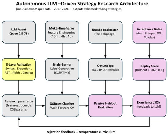
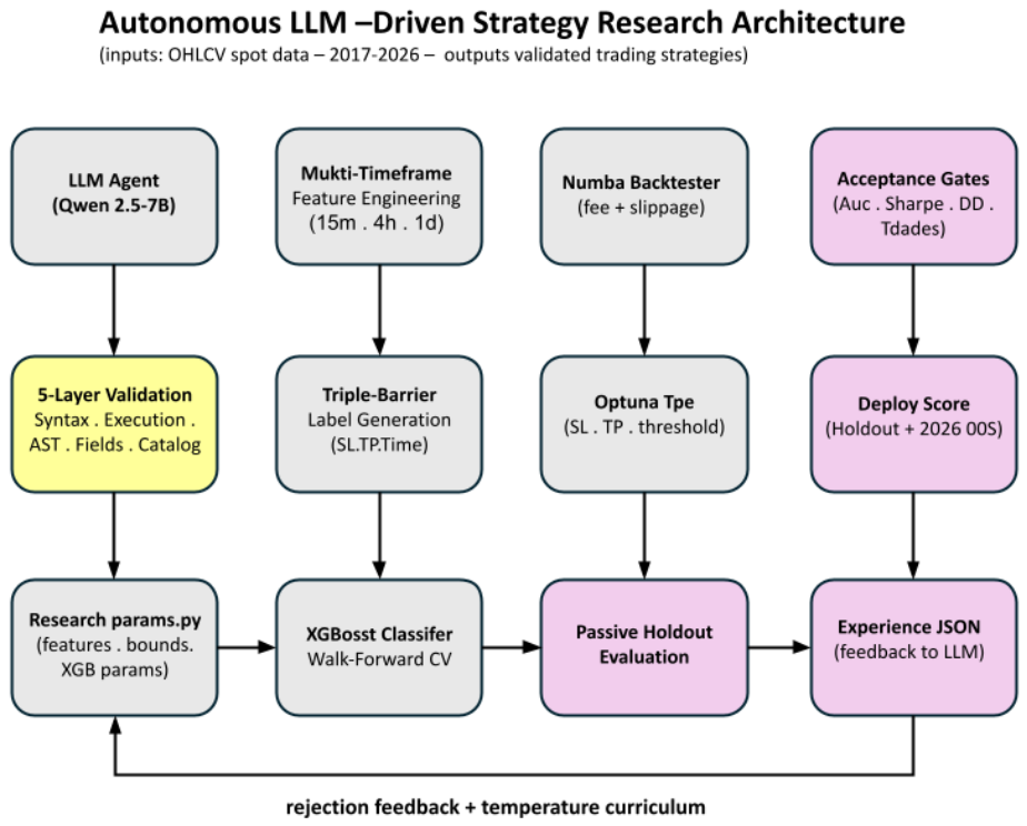


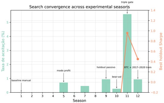
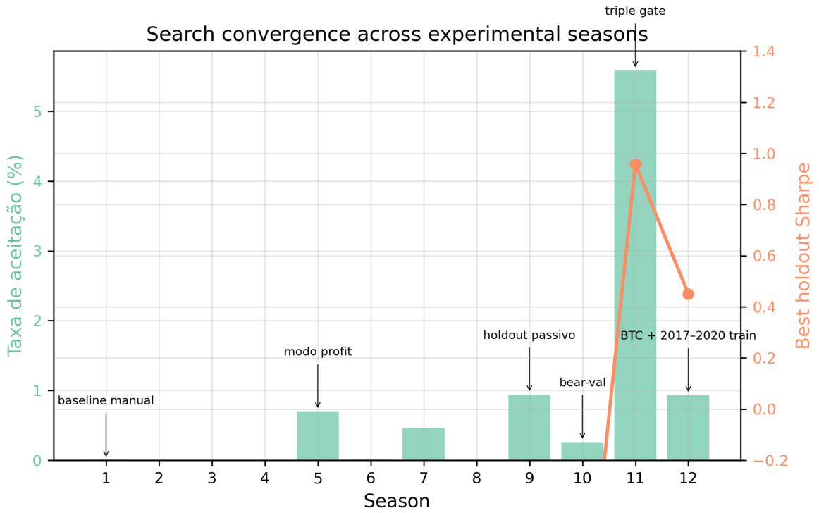
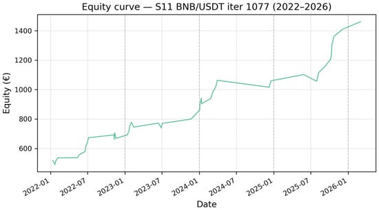
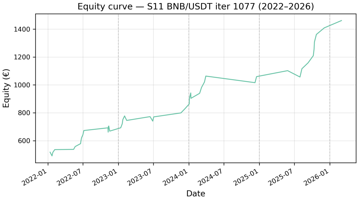
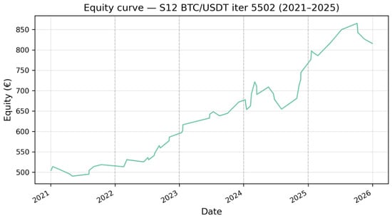
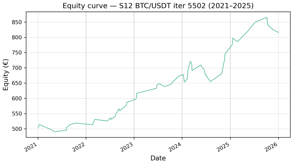
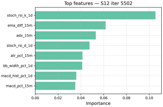
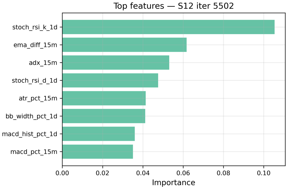
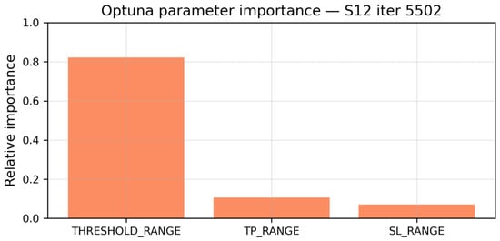
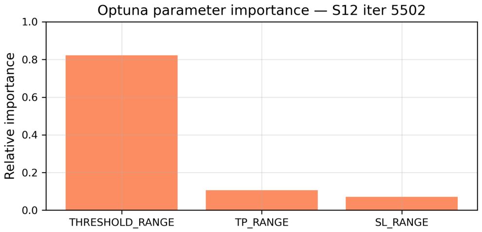
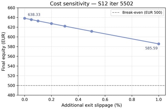
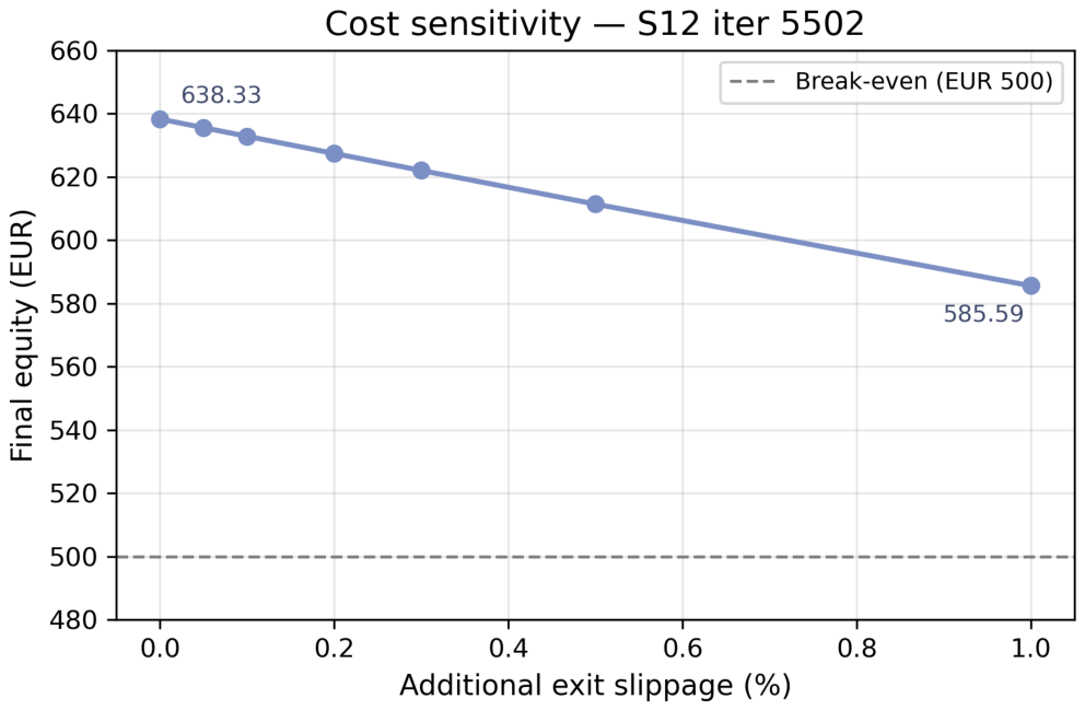
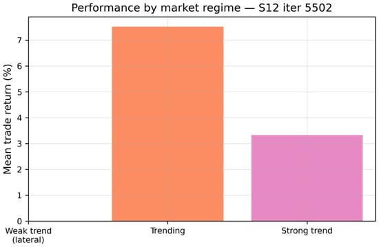
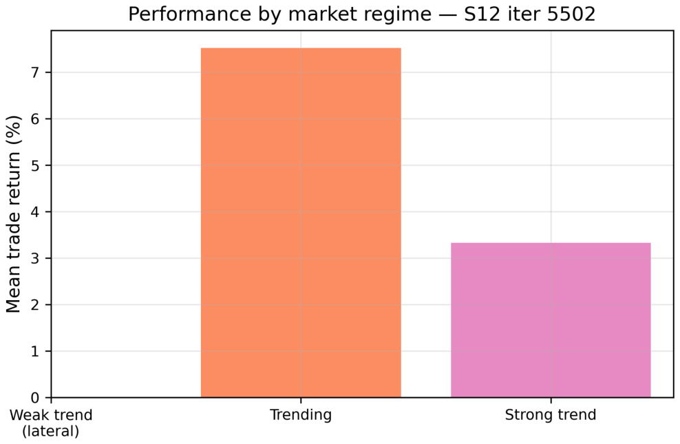

Disclaimer/Publisher’s Note: The statements, opinions and data contained in all publications are solely those of the individual author(s) and contributor(s) and not of MDPI and/or the editor(s). MDPI and/or the editor(s) disclaim responsibility for any injury to people or property resulting from any ideas, methods, instructions or products referred to in the content. |
© 2026 by the authors. Licensee MDPI, Basel, Switzerland. This article is an open access article distributed under the terms and conditions of the Creative Commons Attribution (CC BY) license.