


Abstract
Background: Can predictive algorithms trained on survey data affected by systematic measurement error meet official statistics quality standards? This study examines the tension between design-based inference and algorithmic modelling in poverty estimation, focusing on regressive income underreporting in the Italian shadow economy. Methods: A Monte Carlo microsimulation protocol of 1000 replications is calibrated on ISTAT and EU-SILC 2025 statistics. The shadow economy is formalised as Missing Not At Random measurement error with spatial heteroscedasticity across three Italian macro-regions. Five estimators—design-based, algorithmic, and hybrid—are compared and audited through the QOSU framework. Results: The GREG retains asymptotic design-unbiasedness on undistorted data but exhibits bias up to +29% on observed data, showing that calibration is insufficient under non-ignorable error. Uncalibrated machine learning estimators display systematic bias via shrinkage or amplification, termed statistical hallucination. The Asymmetric Hybrid, with a parameter-free quadratic weighting function, achieves GOLD in five of six domain–indicator combinations; a hold-out validation identifies a reliability threshold of 0.70 as the framework’s domain of validity. Conclusions: Integrating machine learning into official statistics requires an adaptive architecture in which each component’s contribution is modulated by the reliability of the information base. The QOSU framework provides a reproducible protocol for auditing algorithmic estimates under non-ignorable measurement error.
1. Introduction
1.1. Overview
The production of official statistics rests on a compact that is at once mathematical and institutional. Its mathematical dimension is familiar: probabilistic sampling, design-based inference, calibration on known auxiliary population totals. Its institutional dimension is less often made explicit, yet it is no less constitutive. The legitimacy of a national statistical institute—its capacity to inform public policy, to allocate public resources, to shape the terms of political debate—depends on a shared understanding that its estimates are accurate in expectation, transparent in their assumptions, and reproducible in their methods. This compact has served official statistics well for the better part of a century. It is now being tested by a paradigmatic transition whose contours remain only partially understood. The proliferation of big data, administrative registers, and computationally intensive modelling techniques has generated both an opportunity and a hazard. The opportunity is by now well documented. Machine learning methods, particularly ensemble techniques such as gradient boosting and random forests, offer the prospect of finer spatial granularity, faster production cycles, and the ability to extract signal from high-dimensional covariate spaces that classical model-assisted estimators cannot easily accommodate. The hazard is subtler and more consequential.
As Breiman’s celebrated essay on the “two cultures” [1] observed, the design-based and algorithmic traditions rest on different—and in some respects incompatible—epistemological premises. The former prioritizes unbiasedness, interpretability, and the quantification of sampling error; the latter prioritizes predictive accuracy and treats the training set as the ultimate arbiter of performance. When the two traditions are brought into contact, as they increasingly are in the emerging field of algorithmic official statistics, the resulting tension is not merely technical but institutional.
The Italian context provides an unusually clear illustration of these issues. The AROPE indicator (At Risk of Poverty or Social Exclusion) is a composite measure combining monetary poverty, severe material and social deprivation, and very low work intensity. It constitutes a cornerstone of European social policy: the allocation of structural funds, the targeting of welfare programmes, and the evaluation of national reform strategies all depend, to a greater or lesser degree, on the accuracy of AROPE estimates at the territorial level. The macro-regions of Southern Italy—Calabria and Sicilia in particular—are characterized by a high incidence of the shadow economy, a phenomenon documented in the empirical literature on Italian non-observed economic activity [2]. Households in these regions systematically under report their income, and the extent of under-reporting is correlated with income itself: the underreporting mechanism is regressive. The result is a spatially structured measurement error whose variance is not constant across domains and whose mean is systematically negative. Any estimator—design-based or algorithmic—that ignores this structure risks producing biased estimates, with potentially severe consequences for the allocation of public resources.
The present study extends a preliminary investigation presented at the XLVII Annual Scientific Conference of the Italian Association of Regional Science [3]. It develops that work in four complementary directions: it provides a full formalization of the QOSU (Quality of Official Statistical Uncertainty) auditing framework; it implements a Monte Carlo simulation protocol of 1000 replications on a synthetic population of sixteen million micro-units; it proposes a parameter-free quadratic weighting function for the hybrid estimator, eliminating any possibility of data snooping; and it validates the proposed estimator on five additional synthetic domains, strictly disjoint from the calibration domains.
1.2. Background and Related Work
The integration of machine learning into official statistics is the most recent expression of a long-standing tension between model-based and design-based approaches to inference. The classical debate—articulated by Hansen, Madow, and Tepping in the 1970s, revisited by Särndal, and brought to a broader audience by Breiman [1]—concerned the relative merits of randomization-based inference and model-based prediction. Two developments have transformed this debate into an institutional challenge. The first is the sheer volume of data now available, which renders algorithmic approaches computationally feasible in ways inconceivable a generation ago. The second is the growing demand for territorially disaggregated estimates, which cannot always be produced through direct estimation from survey samples and which naturally invite the use of predictive modelling techniques.
Official statistics derive their legitimacy from a set of institutional values—transparency, replicability, accountability, methodological rigour—that are not, in general, natural features of machine learning systems. The European Statistics Code of Practice [4] and its associated Quality Assurance Framework articulate these values in detail: statistical outputs must be based on sound methodology, documented, defensible, and free from systematic error. Machine learning systems, by contrast, are frequently opaque in their internal workings—the “black-box” problem—rarely accompanied by inferential guarantees, and often trained on data whose error structure is poorly characterized. The design-based tradition prioritizes unbiased inference, rests on probability and sampling theory, assumes random sampling with known inclusion probabilities, quantifies sampling error explicitly, achieves high transparency through model-assisted estimators, and operates within established quality frameworks. The algorithmic tradition, by contrast, prioritizes predictive accuracy, rests on empirical risk minimization, assumes that the training data represent future data, often ignores measurement error, is opaque in its internal workings, and operates under ad hoc data governance arrangements.
The methodological crux of the present study is the interaction between algorithmic estimation and non-sampling error. The Total Survey Error framework—formalized by Groves and Lyberg [5]—provides the natural conceptual map. Two sources of non-sampling error are of particular relevance. The first is non-response, understood as a form of missingness in the sense of Rubin [6]. Selected units are absent from the observed sample, and the probability of their absence may or may not depend on their characteristics. Rubin’s classification distinguishes three cases: Missing Completely At Random (MCAR), where the probability of missingness is independent of both observed and unobserved variables; Missing At Random (MAR), where the probability depends only on observed variables; and Missing Not At Random (MNAR), where the probability depends on the unobserved variable of interest. Only the last case is non-ignorable in the technical sense.
The second is measurement error, understood not as absence but as distortion. The unit is present in the sample; it is the reported value that differs from the true value. In the classical formulation of measurement-error theory, the observed variable is modelled as a function of the true variable and an error term, whose properties determine the direction and magnitude of the resulting bias. When the error is non-classical—that is, when it is correlated with the true value—the bias cannot be corrected by simple calibration or by instrumental-variable methods without additional assumptions.
The Italian shadow economy exemplifies the second mechanism, in its non-classical form. Household under-report their income, and the extent of under-reporting is inversely correlated with income. The measurement error is therefore systematic, heteroscedastic, and spatially structured. This is precisely the type of error that invalidates standard calibration techniques and that is most dangerous for machine learning algorithms, because the algorithms, trained to minimize prediction error on the observed data, have no way of distinguishing the signal from the error.
The distinction between missingness and measurement error is frequently blurred in policy-facing discussions of data quality, where non-response and under-reporting are often treated as interchangeable instances of “bad data”. We insist on the distinction because the two mechanisms are not interchangeable. Missingness is addressed through weighting, imputation, or selection models, all of which operate on the probability of inclusion and leave the reported values untouched; measurement error, by contrast, requires latent-variable models, validation samples, or—as in the present study—the design of estimators that are intrinsically robust to the distortion of the reported values.
The consequences for algorithmic auditing are equally divergent. An algorithm trained on data affected by missingness may or may not exhibit bias; when it does, the bias is often detectable through conventional diagnostics. An algorithm trained on data affected by non-classical measurement error will almost certainly exhibit bias, and the bias may remain invisible to the very diagnostics that the analyst would ordinarily employ, because the algorithm has learned the error rather than the phenomenon it distorts. It is precisely this asymmetry—between a problem that announces itself and a problem that does not—that motivates the auditing framework developed in the present study. The failure mode that arises when an estimator learns the measurement error rather than the underlying phenomenon is termed, in this paper, “statistical hallucination”.
The term “statistical hallucination” is introduced by the author and is used within the specific context of algorithmic auditing under non-ignorable measurement error. It should not be confused with the notion of “hallucination” in large language models, which designates the generation of fluent but factually ungrounded content. The analogy is structural rather than substantive: in both cases, apparent coherence coexists with substantive inaccuracy. In classical statistical terminology, the phenomenon corresponds to specification bias under model misspecification.
Given these challenges, there is a pressing need for algorithmic auditing in official statistics. Algorithmic auditing refers to the systematic evaluation of algorithmic systems to assess performance, identify biases, and ensure compliance with quality standards [7]. The QOSU (Quality of Official Statistical Uncertainty) auditing framework proposed in this study provides a multidimensional auditing protocol that evaluates estimates across three critical dimensions: accuracy (Relative Bias), precision (Coefficient of Variation), and homogeneity (Levene’s Test). The framework is not merely a certification tool: as Section 3.4 demonstrates, it also functions as a diagnostic instrument, identifying the reliability threshold below which the proposed estimator ceases to attain its highest certification level.
1.3. Contributions
This study investigates whether advanced machine learning techniques outperform traditional logistic regression and generalized regression estimators in the tracking of poverty under non-ignorable measurement error. Three hypotheses guide the empirical investigation. The first concerns the robustness of design-based inference: the GREG estimator, by virtue of calibration on known auxiliary population variables, is expected to preserve its asymptotic design-unbiasedness—but only under the assumption that the measurement-error mechanism is ignorable. Under non-ignorable error, the estimator is expected to converge to a pseudo-true value that differs from the target. The second hypothesis concerns the behaviour of unconstrained model-based estimators: in domains characterized by high informational opacity, these are expected to manifest a systematic distortion whose direction—amplification or shrinkage—depends on the informational content of the covariates. The third hypothesis concerns the spatial structure of the residual variance, expected to be non-homogeneous across the national territory. A fourth hypothesis concerns the generalizability of the framework: the proposed Asymmetric Hybrid Estimator, by relying on a parameter-free weighting function, is expected to remain applicable outside the domains on which it was calibrated, and the boundaries of this generalizability are expected to be identifiable through the auditing framework itself.
The remainder of the paper is organized as follows: Section 2 develops the methodological framework: the synthetic population, the MNAR underreporting mechanism, the two-stage sampling design, the estimation architectures, and the QOSU classification rules. Section 3 presents and interprets the empirical results. Section 4 discusses the broader implications, and Section 5 concludes this study.
2. Methods
The methodological framework of this study rests on a Monte Carlo microsimulation protocol designed to isolate and quantify the specific contribution of distinct sources of error in poverty estimation under conditions of informational asymmetry and territorial heterogeneity. The protocol extends the preliminary design of Lima [3] through three refinements: a fully specified two-stage stratified sampling design with probability proportional to size; a dual-regime architecture—benchmark and realistic—that separates the effect of measurement error on the design-based and algorithmic components; and the QOSU auditing framework. The protocol adheres to best practice in statistical simulation studies [8].
2.1. Population Synthesis and Data Generating Process
The synthetic population comprises sixteen million micro-units, distributed across three macro-domains in proportions calibrated on the number of Italian households—61% in Lombardia, 28% in Sicilia, and 11% in Calabria—so that the territorial composition of the simulated economy reproduces that of the national one. The three domains were chosen to maximize the heterogeneity of non-sampling error variance, so that the behaviour of the estimators could be observed across a wide range of informational environments. This heterogeneity is quantified by the reliability coefficient φ_d, defined as the proportion of true economic activity that is correctly declared to the statistical authority, calibrated on the most recent ISTAT estimates of the non-observed economy [9]. The coefficient takes values in [0, 1]: φd = 1 corresponds to perfect declaration, φd = 0 corresponds to complete underreporting, and (1 − φd) measures the degree of under-reporting. The coefficient takes the value φ = 0.915 in Lombardia, φ = 0.827 in Sicilia, and φ = 0.810 in Calabria, spanning a range from moderate to severe under-reporting. The interpretation of φd is standard in the literature on the shadow economy [2].
True household income is generated according to a log-normal distribution:
where the following definitions are used:
- ∼ denotes the true (latent) household income for unit i in domain d, expressed in euros per year;
- i indexes the micro-units of domain d, for i = 1, …, Nd
- d ∈ D denotes the domain, with D = Lombardia, Sicilia, Calabria;
- μd and σ2d are, respectively, the mean and the variance of the underlying log-normal distribution.
The log-normal specification is motivated by the empirical regularity that household income exhibits a right-skewed distribution with a pronounced upper tail—a feature that is inadequately captured by symmetric distributions [10,11].
The income so generated is then multiplied by a set of sociodemographic multipliers—education, age, citizenship, and household composition—whose coefficients are calibrated on EU-SILC 2024 medians.
Formally, the household income of micro-unit i in domain d is
where the three multipliers capture, respectively, the effects of the highest educational qualification attained, the age class of the reference person, and the citizenship status of the household, calibrated on EU-SILC 2024 medians.
The parameters μd and σ2d are calibrated so that the simulated mean household income matches the EU-SILC 2025 published values, and the simulated monetary poverty rate—defined at 60% of the national median equivalent income—matches the EU-SILC 2025 targets. The resulting parameter values are reported in Table 1.
Table 1.
Calibrated log-normal parameters by domain.
The equivalent household income is computed using the Modified OECD Equivalence Scale, which adjusts for household composition by assigning weights that reflect economies of scale in consumption:
where the following definitions are used:
- scalai is the equivalence scale of household i;
- is the number of household members aged 14 or older;
- is the number of household members younger than 14.
The equivalent income is , and this is the quantity against which the poverty threshold is applied. The choice of the equivalence scale follows the reference standard in European poverty statistics [10], and provides a standardized basis for comparing economic well-being across households of different compositions.
The marginal distributions of household composition, education, age, and citizenship are calibrated on ISTAT 2024 statistics [12]; conditional income multipliers are derived from EU-SILC 2024 medians. This ensures that the synthetic population reproduces both the marginal distributions and the income–covariate correlations observed in the real data.
The poverty threshold z is defined at 60% of the national median equivalent income [4,11,13].
For the 2025 reference year, this gives z = 13,237 €.
This threshold generates the true Headcount Ratio , defined as the proportion of micro-units in domain d whose equivalent income falls below the poverty line:
where the following definitions are used:
- , denotes the true Headcount Ratio in domain d, expressed as a proportion in [0,1];
- Nd denotes the total population of domain d;
- the index i runs over all micro-units within domain d, for i = 1…N, di = 1…Nd;
- is the true (latent) equivalent household income of micro-unit i in domain d, expressed in euros per year;
- z is the poverty threshold, defined at 60% of the national median equivalent income;
- 1(·) is the indicator function, equal to one when its argument is true and zero otherwise.
Beyond the monetary component, the AROPE indicator is modeled by integrating Severe Material and Social Deprivation (SMSD) and Very Low Work Intensity (VLWI):
where the following definitions are used:
- AROPEi is the indicator of being at risk of poverty or social exclusion for micro-unit i;
- is the indicator of monetary poverty, equal to one when Yi,eq < z;
- SMSDi is the indicator of several material and social deprivation;
- VLWIi is the indicator of very low work intensity;
- ∪ denotes set union;
- The outer 1(·) is the indicator function, equal to one when at least one of the three conditions holds, and zero otherwise.
In other words, a household is classified as at risk of poverty or social exclusion if it experiences monetary poverty, or severe material and social deprivation, or very low work intensity—the three components being complementary rather than mutually exclusive.
The SMSD and VLWI probabilities are modeled via logistic functions that share the same intercept β0 and the same slope β1, but differ by a fixed offset that reflects the empirical regularity that, at any given income level, the probability of very low work intensity is systematically lower than the probability of severe material and social deprivation:
where the following definitions are used:
- is the centred log-income of micro-unit i, expressed in euros per year;
- β0 is the domain-specific intercept; calibrated so that the composite AROPE rate matches the EU-SILC 2025 target [10];
- β1 = −0.45 is the common slope, held fixed across domains and components;
- The constant −0.5 is an offset that applies only to the VLWI specification, reflecting the empirical regularity that, at any given income level, the probability of very low work intensity is systematically lower than the probability of severe material and social deprivation;
- (1 + exp(−x))−1 is the logistic (inverse-logit) function, mapping the real line to the open interval (0, 1).
The offset is not absorbed into the intercept: it is an additional term within the logistic transformation of Equation (7), and it is what differentiates the two probabilities. Equivalently, one may write the two probabilities with separate intercepts and , where = − 0.5; the two formulations are algebraically identical.
2.2. Modeling Non-Sampling Errors
The framework incorporates two conceptually distinct sources of non-sampling error, which must not be conflated. The distinction—between missingness and measurement error—is not merely terminological; it reflects two different mechanisms by which information is lost or distorted, and it carries different implications for the design of corrective estimators.
The first is non-response, which follows a U-shaped function consistent with empirical evidence from household budget surveys [14,15]:
where the following definitions are used:
- P(NonRespi) is the probability that household i does not respond to the survey, expressed as a value in the closed interval [0, 1];
- ri ∈ [0, 1] is the normalized rank of household i in the income distribution, with ri = 0 corresponding to the poorest household and ri = 1 to the wealthiest;
- pbase ∈ 0.10, 0.22, 0.25 is a domain-specific scaling factor, calibrated on the empirical non-response rates for Lombardia, Sicilia, and Calabria, respectively;
- clip (·, 0, 1) denotes truncation of the argument to the unit interval, ensuring that the resulting quantity remains a valid probability in [0, 1].
The base function captures the U-shaped pattern whereby both the poorest and the wealthiest households exhibit lower response propensities, the former because of social stigma and the latter because of privacy concerns. The scaling factor adjusts the average non-response rate to the domain-specific empirical level, so that the effective mean non-response probability ranges from approximately 10% in Lombardia to approximately 25% in Calabria.
The second source is regressive income underreporting, which is not a form of absence but a form of distortion: the unit is present in the sample, yet the reported value differs from the true one. The observed income is modelled as the outcome of a stochastic underreporting process, driven by tax evasion and the shadow economy:
where the following definitions are used:
- δi,d ∈ [0, 1] is the underreporting rate for micro-unit i in domain d—the share of true income that is not declared to the statistical authority;
- is the true (latent) household income, as defined in Equation (1);
- is the observed (reported) household income, which is the quantity available to the estimators;
- is a domain-specific intercept that absorbs the territorial heterogeneity in the intensity of underreporting, calibrated so that the average underreporting rate matches the ISTAT non-observed-economy estimate;
- β1 =−0.10 is the slope parameter, capturing the elasticity of underreporting to income;
- εi,d ~ N(0, τ2) with τ = 0.05 is a stochastic component that captures residual individual-level heterogeneity;
- The constant 10 in Equation (10) is a lower bound on observed income, in euros.
The logistic transformation ensures that the underreporting probability remains bounded between 0 and 1; the domain-specific intercept introduces territorial heterogeneity; and the stochastic component captures residual individual-level variation. The reliability coefficient φd enters the mechanism through the calibration of . The slope parameter β1 is calibrated on Ardizzi et al. [2]: β1 = −0.10. This value remains the only available estimate of the income elasticity of the Italian shadow economy. Its negative sign is not incidental: it captures the regressive nature of underreporting, whereby lower-income households underreport more than higher-income ones, and it is precisely this sign that distinguishes the mechanism from a classical, income-independent measurement error. A sensitivity analysis on the value of β1 shows that the qualitative conclusions are robust to a ±50% variation in the slope parameter.
2.3. Sampling Design and Estimation Architectures
A probabilistic sample is extracted using a two-stage stratified sampling design [8,16]. In the first stage, municipalities—Primary Sampling Units (PSUs)—are selected with probability proportional to size:
where the following definitions are used:
- π1,m is the first-stage inclusion probability of municipality m;
- Nm denotes the population size of municipality m, expressed in number of households;
- M is the set of all municipalities in the population;
- The denominator is the total population size across all municipalities.
In the second stage, a fixed number of households is randomly selected within each selected municipality.
- The design weights are
- di is the design (sampling) weight of household i, expressed as the inverse of its overall inclusion probability;
- π1,m(i) is the first-stage inclusion probability of the municipality m(i) to which household i belongs, as defined in Equation (11);
- π2∣m(i) is the conditional probability of selecting household i in the second stage, given that its municipality m(i) was selected in the first stage.
Four estimation architectures are compared, ranging from the gold standard of official statistics to purely algorithmic approaches. To isolate the effect of measurement error on the design-based and algorithmic components, two variants of the GREG estimator are implemented: a benchmark version, which has access to the true latent values, and a realistic version, which operates only on the observed—and thus distorted—data.
Following Deville and Särndal [17], the GREG adjusts the design weights by minimizing a χ2 distance subject to calibration constraints:
where the following definitions are used:
Σi∈Swixi = Σi∈Uxi
- wi is the calibrated weight of household i, obtained by adjusting the design weight di.
- di is the design weight defined in Equation (12).
- xi is the vector of auxiliary variables observed on household i.
- λ is the vector of Lagrange multipliers of the calibration problem, obtained by solving the system of equations in Equation (14).
- S denotes the set of sampled units, and U denotes the target population. The constraint in Equation (14) requires that the weighted sample totals of the auxiliary variables reproduce the known population totals.
The GREG Benchmark operates on the true latent values and provides the theoretical upper bound of design-based performance in the absence of measurement error.
The GREG Realistic operates on the observed values and represents the operational estimator used in official statistics, vulnerable to non-ignorable measurement error.
The ML-Pure estimator employs a Gradient Boosting Regressor [18,19], trained on sociodemographic variables to predict the observed—and thus distorted—income:
where the following definitions are used:
- is the predicted income for micro-unit i in domain d;
- fGB(X(i,d)| θ) denotes the functional form of the Gradient Boosting Regressor, parameterized by the vector θ;
- θ (bold) denotes the parameter vector of the ML model—the collection of split variables, split points, and leaf values across all trees in the ensemble;
- X(i,d) is the vector of sociodemographic covariates observed on micro-unit i in domain d;
- sd denotes the set of sampled units in domain d, and nd = |sd| is its cardinality;
- The objective in Equation (16) is the empirical squared-error loss, minimized over the parameter vector θ;
- is the resulting headcount estimate, obtained by thresholding the predictions at the poverty line z.
In the notation adopted throughout this paper, boldface is reserved for vectors and matrices, and standard typeface for scalars; any scalar parameter introduced in other sections is denoted by a distinct Greek letter (ξ) to avoid ambiguity with the vector θ.
Gradient boosting is a stagewise additive modelling technique in which each successive tree is fitted to the negative gradient of a loss function; the general treatment is due to Friedman [18], and its place within statistical learning is presented in Hastie et al. [19]. The ML-Pure architecture ignores the sampling design and the calibration weights. A critical limitation is that it trains on distorted income, and therefore may learn the measurement error rather than the underlying phenomenon. The theoretical basis for this failure mode is provided by White’s analysis of maximum likelihood estimation under model misspecification [20]: when the true data-generating process is not in the model class, the estimator converges to a pseudo-true value.
The discrepancy between the ML-Pure and GREG Realistic estimates is defined as , where denotes the estimate in domain d, and denotes the GREG Realistic estimate in domain d.
The Static Hybrid is a convex linear combination with fixed weight:
The weight w = 0.75 is chosen a priori to reflect the methodological priority of design-based inference in official statistics, assigning three times the weight to the GREG estimator that is assigned to the ML component.
The choice is not the result of an estimation procedure; it encodes a prior belief about the relative reliability of the two components under non-ignorable measurement error, and it is held fixed across all domains. The Static Hybrid serves as a benchmark against which the adaptive Asymmetric Hybrid is compared: the point of the comparison is to demonstrate that the adaptive modulation of the weight delivers a gain over a fixed-weight combination, not to propose the fixed weight as an optimal specification.
The proposed Asymmetric Hybrid Estimator determines the weight dynamically as a function of the domain’s reliability coefficient:
with a weighting function specified in parameter-free form:
where the following definitions are used:
- is the estimate produced by the Asymmetric Hybrid Estimator in domain d;
- is the GREG Realistic estimate (Equations (13) and (14)) in domain d;
- is the ML-Pure estimate (Equation (17)) in domain d;
- wd ∈ [0, 1] is the domain-specific weight assigned to the design-based component;
- φd ∈ [0, 1] is the reliability coefficient of domain d.
Only w = simultaneously satisfies monotonicity, the boundary conditions w (0) = 0 and w (1) = 1, boundedness, and parameter-freeness (i.e., absence of calibration).
The specification is chosen on five grounds.
First, it is monotone increasing in φd, so that the design-based component receives more weight in domains with a more reliable information base. Second, it satisfies the boundary conditions w (0) = 0 and w (1) = 1, so that the estimator reduces to the ML-Pure in the limit of complete underreporting and to the GREG Realistic in the limit of perfect declaration. Third, it is bounded in [0, 1] for all admissible φd ∈ [0, 1], so that the weight never becomes negative or greater than unity. Fourth, it is conservative, in that the GREG component receives substantial weight only when the reliability coefficient is high. Fifth, it requires no calibration on any dataset, eliminating any risk of data snooping. A calibrated function would risk overfitting the estimator to the specific domains under study, whereas the parameter-free quadratic form encodes a prior belief about the relative reliability of the two components and can be deployed on any dataset without recalibration. A sensitivity analysis on six alternative parameter-free functional forms is reported in Section 3.3.
2.4. Variance Estimation and Monte Carlo Protocol
Because the Gradient Boosting algorithm does not have a closed-form variance formula, non-parametric bootstrap is applied [15]. The procedure consists of drawing B = 400 bootstrap samples with replacement and computing the variance on the empirical distribution of the B estimates:
where the following definitions are used:
- is the bootstrap variance of the estimator in domain d;
- is the estimate produced in the b-th bootstrap replication, for b = 1…B;
- is the mean of bootstrap estimates;
- B = 400 is the number of bootstrap replicates.
A sensitivity analysis on the number of bootstrap replicates shows that the Coefficient of Variation (CV) estimates stabilize at B = 400, with further increases producing changes of less than 0.1%.
The entire process is executed for R = 1000 Monte Carlo replicates.
A convergence analysis shows that the Monte Carlo Standard Error (MC_SE) stabilizes below 0.001 at R = 1000. The Monte Carlo mean and variance are
where the following definitions are used:
- is the estimate produced in the r-th Monte Carlo replication, for r = 1, …, R;
- R = 1000 is the total number of Monte Carlo replications.
The MSE is decomposed into variance and squared bias:
where VarMC(Ĥd) is the Monte Carlo variance defined in Equation (23), is the Monte Carlo mean defined in Equation (22) and is the true Headcount Ratio, defined in Equation (4).
To assess the clustering effect induced by the two-stage sampling design, the Intraclass Correlation Coefficient (ICC) was computed using the Shrout–Fleiss (1979) estimator [21]:
where MSB is the between-group mean square from a one-way ANOVA on the PSU grouping, MSW is the within-group mean square from the same ANOVA, and is the average cluster size.
The calibration procedure ensures that the simulated ICC equals 0.28, consistent with the range reported in the household survey literature [22]. A sensitivity analysis over the interval ICC ∈ [0.10, 0.75] is reported in Section 3.6.
2.5. The QOSU Auditing Framework
The QOSU framework is proposed to evaluate estimates across three dimensions.
Accuracy is measured by the Relative Bias (RB):
where RBd is the Relative Bias of the estimator in domain d, expressed as a percentage; is the Monte Carlo mean of the estimator defined in Equation (22); and is the true Headcount Ratio, defined in Equation (4).
The Relative Bias has a tolerance threshold of |RBd| < 8%.
This threshold reflects the quality standards for key social indicators established by Eurostat, which require that RB for poverty indicators not exceed 5–10% for official publication.
Precision is measured by the Coefficient of Variation:
where MCSD and MCmean denote the standard deviation and mean of the estimator across the R = 1000 Monte Carlo replications, defined in Equations (22) and (23).
The threshold CV% < 15% is set consistently with the precision requirements for domain-level estimates in the European Statistical System. Eurostat’s quality standards for social statistics require that the Coefficient of Variation for domain-level poverty indicators remains below 15% for reliable publication, and the ESS Quality Assurance Framework [4] identifies this value as the operational ceiling above which an estimate is considered too imprecise for policy use. The threshold is therefore not an arbitrary convention but an institutional parameter, adopted here to ensure that the QOSU classification is aligned with the criteria that govern the publication of official poverty statistics in the European Union. Homogeneity of residuals is verified through Levene’s Test [23].
The explicit decision rules are as follows: FAIL if CV% ≥ 15; GOLD if CV% < 15 and ∣RB%∣ < 8; SILVER otherwise. The classification is asymmetric by design: accuracy is prioritized over precision.
Table 2 summarizes the above classification criteria.
Table 2.
QOSU classification criteria.
The classification scheme is asymmetric by design: accuracy is prioritized over precision, reflecting the decision-theoretic principle that the cost of a biased estimate exceeds the cost of a slightly less precise one. Following the standard convention of statistical quality control and hypothesis testing [24], we adopt the null hypothesis H0: the estimator is valid. Type I error is the probability of classifying a truly unbiased estimator as FAIL; Type II error is the probability of classifying a truly biased estimator as GOLD. The coverage rate of the 95% confidence intervals is also reported.
3. Results
The empirical analysis that follows is based on R = 1000 Monte Carlo replications, executed over a synthetic population of sixteen million micro-units calibrated on the most recent ISTAT and EU-SILC 2025 official statistics. Scenario A grants the design-based estimator access to the true latent values, isolating the effect of the MNAR measurement-error mechanism on the algorithmic component alone. Scenario B restricts all estimators to the observed values Yobs, mirroring the informational constraints that govern real survey production.
3.1. The Benchmark Case
The performance of the GREG estimator under the benchmark case confirms that calibration on known auxiliary population totals, when combined with access to undistorted information, delivers asymptotically design-unbiased estimates. The Relative Bias remains uniformly small—−4.63% in Lombardia, −1.74% in Sicilia, and −2.97% in Calabria—well within the ±8% tolerance threshold. The Coefficient of Variation sits comfortably below the 15% ceiling in every domain, with the highest value, 9.26%, recorded in Lombardia. The estimator attains a GOLD rating across the board. The pattern of bias is not random: in every domain, the GREG Benchmark slightly underestimates the true Headcount Ratio. This is a structural property of the estimator: as the log-normal income distribution is sampled with the 60% median threshold fixed, small-sample fluctuations in the lower tail translate into a mild negative bias. The corollary is equally important: the robustness of the GREG is contingent upon the ignorability of the error mechanism.
3.2. The Realistic Case
Table 3 presents the performance of the five estimators in the Calabrian domain (φ = 0.810), the most challenging informational environment. The GREG Realistic, which in Scenario A exhibited a Relative Bias of −2.97%, now produces a Relative Bias of +29.28%—nearly four times the tolerance threshold. The calibration equation adjusts the design weights so that the weighted sample totals reproduce the known population totals for the auxiliary variables. This correction is effective when the discrepancy between sample and population arises from sampling variability, or when the missingness mechanism is ignorable in the Rubin sense [6]. It is, however, powerless against a systematic distortion in the variable of interest itself.
Table 3.
Calabria, monetary poverty (φ = 0.810).
The behavior of the ML-Pure estimator is equally instructive, though in the opposite direction. With a Relative Bias of −37.35%, the ML-Pure systematically underestimates poverty. The Gradient Boosting Regressor learns to predict the conditional mean of the observed distribution; because the conditional mean of a right-skewed distribution is situated well above the median, the predicted incomes cluster toward the upper portion of the distribution, and fewer households than appropriate are classified as poor. The result is a systematic downward bias, driven by shrinkage toward the conditional mean. The direction of the algorithmic bias depends on the informational environment. When informative covariates are available, the bias is negative—shrinkage; when the algorithm is forced to rely on covariates with little predictive power, it learns the measurement error itself, and the bias is positive—amplification. It is in this sense that the term “statistical hallucination” is best understood: not as a single numerical signature, but as a family of systematic distortions whose common denominator is the dissociation between apparent precision and substantive accuracy. The Static Hybrid estimator exhibits an intermediate Relative Bias of +12.62%. This demonstrates that a simple convex combination of a calibrated estimator and an algorithmic estimator does not, in itself, neutralise the effects of non-ignorable error. The two components share a common exposure to the distorted information base. The Asymmetric Hybrid, with w = 0.656 in Calabria, produces a Relative Bias of +6.36% on monetary poverty and +4.47% on the AROPE indicator (see Table 4). On both indicators, the estimator attains a GOLD rating. The MSE falls from 0.015585 (ML-Pure) to approximately 0.000679 (Asymmetric Hybrid), a reduction of more than 95%.
Table 4.
Calabria, AROPE (φ = 0.810).
The divergence between the monetary and AROPE results deserves comment. Because SMSD and VLWI are themselves correlated with income—but not perfectly so—the composite indicator is less sensitive to the systematic distortion in the monetary component. The AROPE indicator thus provides a more favourable terrain for the deployment of hybrid estimators, while the monetary indicator remains the more demanding test bed.
3.3. The Proposed Estimator
Table 5 reports the sensitivity analysis on six alternative parameter-free weight functions.
Table 5.
Weight function sensitivity.
Three observations emerge from this table. The concave forms—φ0.5 and φ—underweight the GREG component and produce Relative Biases consistently above the tolerance threshold. The convex form—φ3—overweights the GREG and overshoots in Sicilia. The quadratic form φ2 sits precisely at the optimum, achieving GOLD in five of the six combinations. The quadratic form satisfies the boundary conditions w (0) = 0 and w (1) = 1, is monotone increasing, and grows slowly for low values of φ. It does not require calibration on the validation domains, and therefore it does not expose the estimator to data snooping. It does not contain free parameters that could be tuned to improve in-sample performance. And it does not depend on external information beyond φ_d itself. The parameter-free nature of w(φ) = φ2 is, in short, the methodological counterpart of the reproducibility principle that underpins official statistics.
Figure 1 presents the same results graphically. The figure makes immediately visible that the concave and convex forms bracket the quadratic optimum, and that the quadratic form is the only specification that stays close to the tolerance band across all three domains.
Figure 1.
Weight function sensitivity across six parameter-free functional forms. Note: Relative Bias (%) of the Asymmetric Hybrid Estimator under six alternative weight functions computed separately for Lombardia, Sicilia, and Calabria on monetary poverty. The dashed gold lines indicate the ±8% QOSU accuracy threshold. Only w = ϕ2 satisfies simultaneously monotonicity, the boundary conditions w (0) = 0 and w (1) = 1, boundedness, and parameter-freeness. Source: Author’s elaboration on microsimulation data.
3.4. Domain of Validity Under Genuine Out-of-Sample Conditions
The parameter-free weight function w(φ) = φ2 requires no calibration on any dataset. To assess its behaviour outside the three validation domains, we generated five independent synthetic populations with φ ∈ 0.40, 0.50, 0.60, 0.70, and 0.75, all calibrated on common targets—mean household income of €37,000, poverty rate of 0.35, AROPE rate of 0.44, base non-response of 0.18—so that φ is the only varying parameter. Each population was subjected to the same MNAR underreporting mechanism, the same U-shaped non-response pattern, and the same two-stage stratified sampling design as the main simulation. R = 200 Monte Carlo replications were executed per domain, each on a synthetic population of one million micro-units.
Table 6 reports the results. The Asymmetric Hybrid attains GOLD certification only in three of ten domain–indicator combinations, all concentrated at φ ≥ 0.70.
Table 6.
Hold-out validation of the Asymmetric Hybrid Estimator.
The pattern is monotone in φ: the Relative Bias declines from +106.7% at φ = 0.40 to +4.3% at φ = 0.75 for the monetary indicator, and from +73.6% to +4.0% for AROPE.
The mechanism is structural rather than stochastic. As φ decreases, the GREG Realistic bias grows monotonically (from +35.7% at φ = 0.75 to +111.6% at φ = 0.40), while the ML-Pure bias changes sign (from −36.0% at φ = 0.75 to +105.8% at φ = 0.40). At φ = 0.75, the two biases are almost exactly opposite and cancel under the φ2 weighting. Below φ = 0.70, the cancellation fails because the GREG bias grows faster than the ML-Pure bias can compensate. This result defines the domain of validity of the proposed framework. The empirical threshold φ ≥ 0.70 corresponds to a shadow economy below 30% of value added—a condition satisfied by all Italian macro-regions and by the overwhelming majority of European Statistical System settings. For contexts with severe underreporting (φ < 0.70), the framework does not provide a corrective remedy; it provides a diagnostic. The QOSU classification correctly assigns SILVER or FAIL ratings, signalling that the adaptive hybrid cannot recover the true headcount without an explicit correction based on φ. This is precisely the behaviour that an auditing framework should exhibit: it does not hide its own limitations, and it produces an explicit, reproducible, and institutionally actionable warning when the conditions of applicability fail. Figure 2 presents the results graphically.
Figure 2.
Hold--out validation of the Asymmetric Hybrid Estimator. Panel (a) Monetary poverty. Note: Relative Bias (%) of the GREG Realistic, ML-Pure, and Asymmetric Hybrid estimators as a function of φ ∈ 0.40, 0.50, 0.60, 0.70, and 0.75. The vertical dotted line marks φ = 0.70. The dashed gold lines indicate the ±8% QOSU accuracy threshold. Source: Author’s elaboration on microsimulation data. Panel (b) AROPE. Same notation as Panel (a). Note: GOLD certification is attained only in three of ten domain–indicator combinations, all concentrated at φ ≥ 0.70. Source: Author’s elaboration on microsimulation data.
3.5. External Validation Against ISTAT
To provide indirect external validation, the simulated AROPE estimates are compared with the official ISTAT AROPE published values (see Table 7).
Table 7.
Comparison with ISTAT AROPE 2025.
This comparison cannot replace direct validation on real microdata—which is prohibited by confidentiality regulations—but it provides a benchmark against which the simulated aggregates can be assessed. The absolute differences are uniformly small—between 0.010 and 0.037—and fall within the tolerance thresholds of the QOSU framework, providing initial evidence of the external validity of the simulation design.
3.6. QOSU Certification: Inferential Validity and Rating Summary
The evaluation of estimator reliability in the presence of non-ignorable error raises a subtle question of statistical methodology. The QOSU framework classifies estimators on the basis of Relative Bias and Coefficient of Variation, but the classification operates on a point estimate of the bias, which is itself subject to Monte Carlo variability. What, then, is the probability that the framework misclassifies an estimator? And how does this probability compare with the coverage properties of the confidence intervals produced by each estimator? To address these questions, we report two complementary metrics. The first is the operational Type I/II error rate, defined, following the convention of statistical quality control, as the fraction of Monte Carlo replications in which the classification deviates from the classification that would be obtained on the basis of the true mean bias. The second is the coverage rate of the 95% confidence intervals, defined as the fraction of intervals that contain the true Headcount Ratio. Table 8 reports the results.
Table 8.
Type I/II errors and Coverage Rate (H0 = estimator valid).
The coverage rate discriminates cleanly between estimators whose confidence intervals are correctly calibrated and those whose intervals fail to contain the target.
Figure 3 presents the two metrics graphically. The GREG Benchmark and the Asymmetric Hybrid both achieve 100% coverage. The GREG Realistic and the ML-Pure, by contrast, achieve 0% coverage on monetary poverty: their confidence intervals are narrow, but they are centred on a biased point, and the target lies outside the interval in every replication. The coverage rate is, in this respect, the more informative of the two metrics, because it directly addresses the practical question that matters for policy: does the interval reported by the analyst contain the quantity of interest? The Type II error rate—the failure to detect a genuinely biased estimator—is the more consequential metric from a governance perspective, because it corresponds to an unwarranted certification.
Figure 3.
Inferential validity of the estimators. Panel (a): Coverage rate of the 95% confidence intervals for the five estimation architectures on monetary poverty and AROPE. Note: The dashed green line indicates the nominal 95% coverage. Source: Author’s elaboration on microsimulation data. Panel (b): Operational Type I (false FAIL) and Type II (false GOLD) error rates (%) for monetary poverty, computed under H0: estimator valid. Note: Type I error is the probability of classifying a truly unbiased estimator as FAIL; Type II error is the probability of classifying a truly biased estimator as GOLD. Type II errors are more consequential from a governance perspective, because a false GOLD certifies a biased estimate and exposes the institution to the associated risks of resource misallocation. All values are percentages. Source: Author’s elaboration on microsimulation data.
From a governance standpoint, Type II errors are more severe than Type I errors: the former lead to the certification of biased estimates, with the associated risks of misallocation of resources; the latter lead to excessive caution, which is a lesser institutional evil. The QOSU framework does not eliminate this asymmetry; it renders it explicit and quantifiable. Taken together, the Type I/II analysis and the coverage analysis suggest that the QOSU framework should be interpreted not as a definitive certification, but as a probabilistic statement of quality. The probabilistic character of the certification does not prevent the ratings from being informative at the aggregate level.
Table 9 consolidates the QOSU ratings assigned to each estimator across the three Italian macro-regions and the two indicators, providing a compact overview of the comparative performance of the five estimation architectures under the realistic scenario.
Table 9.
QOSU rating summary across the three Italian macro-regions.
The pattern confirms that the adaptive modulation of the weight between the design-based and the algorithmic components delivers a substantial improvement over both the fixed-weight Static Hybrid and the two pure estimators.
The Asymmetric Hybrid attains GOLD in five of the six domain–indicator combinations, and the sole SILVER outcome—monetary poverty in Lombardia—corresponds to a Relative Bias that lies only marginally above the tolerance threshold, in the domain where the reliability coefficient is highest and the algorithmic component receives the smallest weight.
3.7. Sensitivity Analyses: Missingness Mechanisms, ICC, and Bootstrap Stability
Three additional sensitivity analyses complement the main results. The first concerns the missingness mechanism. Under MCAR, the naive estimator—operating on the surviving sample without correction—exhibits a Relative Bias of approximately zero in every domain; under MAR, the bias is small but non-zero, between −0.09% and −0.28%; under MNAR, where the probability of non-response depends on the income rank, the naive estimator exhibits a Relative Bias of approximately −28%, confirming that non-ignorable missingness, like non-ignorable measurement error, produces a systematic distortion that is not corrected by simple reweighting. A GREG-like correction based on the alignment of the mean partially mitigates the bias to approximately −5.6%, but it does not eliminate it. This contrast between MCAR, MAR, and MNAR provides empirical confirmation of the theoretical distinction between missingness and measurement error, and reinforces the methodological point that the two problems require distinct diagnostic and corrective strategies. The second analysis concerns the Intraclass Correlation Coefficient.
The ICC has been recalculated from the simulated two-stage design, yielding a value of 0.28, consistent with the range of 0.10–0.30 typically reported in the household survey literature [22].
The sensitivity of the CV% and QOSU ratings to variations in the ICC has been verified across the interval [0.10, 0.75]. The qualitative conclusions are robust: the Asymmetric Hybrid maintains its GOLD rating on both monetary poverty and AROPE across the entire range of ICC values. The third analysis concerns the stability of the bootstrap procedure: the Coefficient of Variation estimates stabilise at B = 400, with further increases producing changes of less than 0.1%.
Table 10 reports the sensitivity analyses for the bootstrap procedure, the convergence, the missingness mechanism, the intraclass correlation coefficient, and ICC ∈ [0.10,0.75].
Table 10.
Sensitivity analyses.
The Levene test for spatial heteroscedasticity rejects the null hypothesis of homoscedasticity at the 5% level in all pairwise comparisons on both indicators. The overall test is significant at p < 0.0001. The only borderline case is the Sicilia–Calabria comparison on monetary poverty (p = 0.0313), which suggests that the two Southern domains share a sufficiently similar structure of residual variance that the test distinguishes them with less power. The discrepancy between the ML-Pure and GREG Realistic estimates is systematically negative in every domain, ranging from −0.086 in Lombardia to −0.289 in Sicilia regarding monetary poverty. The pattern is striking: the discrepancy is largest in Sicilia, where φ = 0.827 places the domain in an intermediate position between the two extremes.
4. Discussion
The empirical evidence presented in Section 3 converges on a single, coherent picture of how design-based inference and algorithmic modelling respond to non-ignorable measurement error. The contrast between the GREG Benchmark and the GREG Realistic delineates the boundary condition beyond which the classical apparatus of design-based inference ceases to operate. On uncontaminated data, the GREG Benchmark attains GOLD certification in every domain, confirming the theoretical expectation that calibration on known auxiliary population totals delivers asymptotically design-unbiased estimates when the information base is intact. Once regressive income underreporting is applied, however, the same estimator produces a relative bias of up to +29%, and the calibration constraints prove powerless against a systematic distortion in the variable of interest itself. What the comparison identifies is not a paradox but an assumption—the ignorability of the error mechanism—that design-based inference silently relies upon and that official statistics can no longer take for granted as administrative and survey data become increasingly affected by non-compliance, under-reporting, and deliberate underreporting. Under MNAR measurement error, the estimator converges to a pseudo-true value, and the bias does not diminish with sample size. The methodological implication for algorithmic auditing follows directly: an audit cannot confine itself to verifying the internal consistency of the estimator, but must also establish whether the error mechanism is ignorable and, when that condition fails, deploy estimators designed to be robust to its violation. The behaviour of the algorithmic component adds a second dimension to this picture, and one that is less intuitive than the first. When informative covariates are available, the Gradient Boosting Regressor shrinks its predictions toward the conditional mean and produces a downward bias; when the covariates carry little predictive content, the algorithm fits the measurement error itself and the bias becomes positive. Both patterns fall within what this paper terms statistical hallucination—a family of systematic distortions in which apparent precision coexists with substantive inaccuracy, and whose direction is not a stable property of the algorithm but a function of the informational environment. The practical consequence for auditing is that a diagnostic based solely on the comparison between predicted and observed values may fail to detect the distortion, because the distortion is absorbed in the relationship between the algorithm and its covariates. The QOSU framework addresses this class of failures through the joint inspection of relative bias and coverage rate: the coverage rate discriminates between estimators whose confidence intervals are correctly calibrated and those whose intervals do not cover the target. The GREG Benchmark and the Asymmetric Hybrid both attain 100% coverage, whereas the GREG Realistic and the ML-Pure attain 0% coverage on monetary poverty, their intervals being narrow but centred on a biased point.
Against this background, the performance of the proposed Asymmetric Hybrid Estimator with weight function w(φ) = φ2 provides the constructive counterpart to the diagnostic findings. In the validation on the three Italian macro-regions, five of the six domain–indicator combinations attain GOLD, and the only SILVER outcome is monetary poverty in Lombardia, narrowly exceeding the tolerance threshold. The improvement over the fixed-weight Static Hybrid is particularly instructive: it confirms that the adaptive modulation of the weight, rather than the mere averaging of the two components, is what delivers the gain in accuracy, and that a convex combination of two estimators sharing a common exposure to the distorted information base cannot by itself transcend the informational limitations from which both suffer.
The estimator’s performance proves robust to the specification of the weight function, to the level of the intraclass correlation coefficient, and to the number of bootstrap replicates. Its coverage rate of 100% is consistent with the theoretical expectation for an unbiased estimator, and its Type I error rate is bounded by the Monte Carlo variability in the estimated bias.
The generalizability of the framework was tested on ground that lies strictly outside the conditions under which the estimator was calibrated. The genuine out-of-sample validation reported in Section 3.4, conducted on five synthetic domains with φ ∈ 0.40, 0.50, 0.60, 0.70, 0.75, shows that the Asymmetric Hybrid Estimator attains GOLD certification only in three of ten domain–indicator combinations, all concentrated at φ ≥ 0.70. The Relative Bias declines monotonically as φ increases, and the empirical threshold φ = 0.70—corresponding to a shadow economy of 30% of value added—marks the boundary below which the compensation mechanism between the design-based and algorithmic components ceases to operate. This result defines the domain of validity of the framework rather than undermining it. The threshold is satisfied by all Italian macro-regions and by the overwhelming majority of European Statistical System settings; for contexts with severe underreporting, the QOSU framework does not provide a corrective remedy but a diagnostic, signalling explicitly that the adaptive hybrid cannot recover the true headcount without an additional correction based on φ. The framework thereby renders its own limitations visible and institutionally actionable, rather than concealing them behind an unwarranted certification.
Three implications emerge from these findings, and they are closely intertwined. The first concerns the design of hybrid architectures and the methodological value of reproducibility. The choice of a parameter-free functional form for the weight function is not merely a technical convenience: a calibrated weight function would risk overfitting the estimator to the specific domains under study, whereas the parameter-free form encodes a prior belief about the relative reliability of the two components and can be deployed on any dataset without recalibration. The quadratic form satisfies the boundary conditions w (0) = 0 and w (1) = 1, is monotone increasing, and grows slowly for low values of φ, so that the design-based component receives substantial weight only when the reliability of the information base justifies it. The second implication concerns the QOSU framework as an instrument of governance. Its decision rules are explicit, and its asymmetry—the prioritization of accuracy over precision—reflects the principle that the cost of a biased estimate, in terms of resource misallocation, exceeds the cost of a slightly less precise one. The Type I/II analysis reported in Section 3.6 renders this asymmetry explicit and quantifiable: Type II errors are more consequential than Type I errors, because a false GOLD certifies a biased estimate and exposes the institution to the associated risks, whereas a false FAIL leads to additional caution, whose institutional cost is comparatively lower. The framework does not eliminate this asymmetry, and its classification becomes unstable near the tolerance thresholds. It should therefore be read as a probabilistic statement of quality rather than as a definitive certification—but it nonetheless provides a transparent and replicable protocol for the audit of algorithmic systems in the public sector. The third implication concerns the consequences of estimation error for policy. A precise but biased estimate of poverty would lead to the misallocation of structural funds and would exacerbate territorial inequalities. The framework is not specific to poverty estimation, nor to Italy; it can be applied to any setting in which algorithmic methods operate on data affected by non-sampling error, and it can be adopted across national statistical systems as a shared protocol for algorithmic auditing.
The scope of these results is bounded, however, by several constraints that deserve explicit acknowledgment. The most consequential is the reliance on synthetic data. The population is calibrated on official ISTAT and EU-SILC 2025 statistics, and the calibration ensures that the synthetic population reproduces the salient features of the Italian territorial distribution of income, poverty, and informality; it cannot, however, reproduce the full complexity of the real data-generating process. Access to ISTAT microdata is restricted by Regulation (EU) 2019/1700 and by the Italian Statistical Confidentiality Act, and their use in simulation studies that modify their structure is not permitted. Moreover, the evaluation of estimator performance under MNAR measurement error requires knowledge of the latent true values, which are unobservable in real surveys. Synthetic data provide the only controlled environment in which the target is known by construction, and this constraint defines the scope of the exercise rather than a limitation that can be removed through alternative data sources. A second constraint concerns the treatment of the reliability coefficient φ_d as a territorial constant rather than as a trajectory. The shadow economy exhibits adaptive dynamics over the business cycle, and the extent of underreporting may vary with macroeconomic conditions; a dynamic extension, in which φ_d is modelled as a stochastic process and the weight function is updated as new information becomes available, would represent a natural next step. Relatedly, the empirical threshold φ = 0.70 identified in Section 3.4 is itself a function of the specific simulation design—the common target values, the calibration of β1, and the choice of R = 200 replications—and while the qualitative conclusion that the framework has a domain of validity bounded away from φ = 0 is robust, the precise location of the threshold may shift under alternative parameterizations. A third constraint concerns the scope of the simulation, which is calibrated on three Italian macro-domains and a single reference year; generalization to other statistical systems, to sub-regional levels, and to multiple reference years requires the calibration of φd on different data sources and different reliability estimates, and it may reveal patterns of heterogeneity that the present design does not capture. A fourth constraint concerns the algorithmic architecture: the ML component is implemented using a Gradient Boosting Regressor [18], and the empirical results are specific to that choice.
Alternative architectures might yield different biases, and the optimal weight function might depend on the algorithmic architecture. The qualitative conclusion of the study is a general property of empirical risk minimization and is therefore robust to the choice of algorithm; the quantitative magnitudes reported here should be read as illustrations rather than as universal constants.
The most promising direction for future work is the application of the QOSU framework to real microdata, once access is granted under the appropriate confidentiality protocols. Beyond this, three extensions appear particularly valuable: the development of a dynamic version of the framework, in which the reliability coefficient evolves over time; the systematic comparison of alternative algorithmic architectures, carried out to assess whether the weight function w(φ) = φ2 remains optimal across different inductive biases; and the extension of the framework to indicators beyond AROPE and to countries in which the shadow economy operates through mechanisms different from the Italian case. The broader methodological point is that the integration of machine learning into official statistics need not be framed as a choice between the design-based and the algorithmic paradigms. It can be framed, more productively, as the design of an adaptive architecture in which the contribution of each paradigm is modulated by the reliability of the information base. The QOSU framework provides the certification apparatus; the Asymmetric Hybrid provides the operational methodology. Together, they constitute a reproducible and governable protocol for the production of machine-learning-assisted poverty estimates in official statistics.
5. Conclusions
This study has investigated the integration of machine learning into the production of official statistics through a Monte Carlo microsimulation protocol calibrated on ISTAT and EU-SILC 2025 statistics, proposing the Asymmetric Hybrid Estimator and the QOSU auditing framework for the certification of algorithmic estimates under non-ignorable measurement error. The empirical evidence confirms that design-based inference preserves its asymptotic design-unbiasedness only under the assumption of ignorable error, and that this assumption fails when households conceal income in a manner correlated with their position in the income distribution. Under regressive income underreporting, the GREG Realistic converges to a pseudo-true value that differs systematically from the target, exhibiting a relative bias of up to +29%—a bias that does not diminish with sample size. The behaviour of the algorithmic component is more nuanced still: unconstrained machine-learning estimators display a systematic distortion whose direction depends on the informational content of the covariates, shrinking predictions toward the conditional mean when informative covariates are available and amplifying the measurement error when they are not. Both patterns fall within what this paper terms statistical hallucination, and both would remain invisible to diagnostics that rely solely on the comparison between predicted and observed values. The spatial structure of the residual variance, finally, is non-homogeneous across the national territory in a manner associated with the geographical distribution of the shadow economy.
These findings converge on a single methodological conclusion: the integration of machine learning into official statistics requires an adaptive architecture in which the contributions of the design-based and algorithmic components are modulated by the reliability of the information base. The proposed Asymmetric Hybrid Estimator provides such an architecture through a parameter-free quadratic weight function, attaining GOLD certification in five of the six domain–indicator combinations in the primary validation and 100% coverage. Its performance is robust to the specification of the weight function, to the level of the intraclass correlation coefficient, and to the number of bootstrap replicates. The genuine out-of-sample validation on five additional synthetic domains identifies the empirical reliability threshold of 0.70 as the boundary below which the framework ceases to attain GOLD certification, and it thereby renders the framework’s domain of validity explicit rather than implicit: the QOSU classification does not conceal the framework’s limitations, but renders them institutionally actionable.
The QOSU auditing framework supplies the certification apparatus that makes such a protocol reproducible across statistical systems. It translates abstract criteria of statistical quality into a decision-theoretic classification, makes the probability of misclassification explicit, and establishes a direct link between statistical quality and institutional acceptability. The framework is specific neither to poverty estimation nor to Italy; it can be applied in any setting in which algorithmic methods operate on data affected by non-sampling error.
As algorithmic methods become part of the routine production of official statistics, the questions of transparency, replicability, and accountability that the design-based paradigm has addressed for the better part of a century must be reformulated in a manner compatible with the new methods. The QOSU framework offers one such reformulation. Whether it will prove sufficient to govern the next generation of machine-learning-assisted statistics is an open question—and, given the pace at which the informational environment is changing, an urgent one.
Funding
This research received no external funding.
Institutional Review Board Statement
Not applicable.
Informed Consent Statement
Not applicable.
Data Availability Statement
All data were generated synthetically and can be fully reproduced using the Python 3.9 simulation code, which is available upon request from the corresponding author.
Acknowledgments
The author thanks the three anonymous reviewers for their careful and constructive assessment, which substantially improved the methodological rigour and empirical grounding of the manuscript. The author is grateful to the participants of the XLVII Annual Scientific Conference of the Italian Association of Regional Science for their valuable feedback on an earlier version of this work. Gratitude is extended to the Editorial Team of Analytics for the opportunity to contribute to this journal. During the preparation of this manuscript, the author used generative AI tools exclusively for language editing and paraphrasing of text originally drafted by the author. No generative AI tool was used to generate scientific content, formulate hypotheses, design the simulation protocol, analyse the data, or interpret the results. The author has reviewed and verified all content and takes full responsibility for the integrity and accuracy of the work. All materials supporting the analysis—including the simulation code, the synthetic datasets, the raw Monte Carlo outputs, and the revision history of the manuscript—are available to the Editorial Office on request.
Conflicts of Interest
The author declares no conflicts of interest.
Abbreviations
The following abbreviations are used in this manuscript:
| AROPE | At Risk of Poverty or Social Exclusion |
| CV | Coefficient of Variation |
| GREG | Generalized Regression Estimator |
| ICC | Intraclass Correlation Coefficient |
| MAR | Missing At Random |
| MCAR | Missing Completely At Random |
| ML | Machine Learning |
| MNAR | Missing Not At Random |
| MSE | Mean Squared Error |
| OECD | Organization for Economic Co-operation and Development |
| PPS | Probability Proportional to Size |
| PSU | Primary Sampling Unit |
| QOSU | Quality of Official Statistical Uncertainty |
| RB | Relative Bias |
| SMSD | Severe Material and Social Deprivation |
| VLWI | Very Low Work Intensity |
References
- Breiman, L. Statistical Modeling: The Two Cultures. Stat. Sci. 2001, 16, 199–231. [Google Scholar] [CrossRef] [Scilit]
- Ardizzi, G.; Petraglia, C.; Piacenza, M.; Turati, G. Measuring the Underground Economy with the Currency Demand Approach: A Reinterpretation of the Methodology, With an Application to Italy. Rev. Income Wealth 2014, 60, 747–772. [Google Scholar] [CrossRef] [Scilit]
- Lima, R. Stimatori Design-Based contro Algoritmi Machine Learning per il Divario Nord-Sud della Povertà Italiana. In Proceedings of the XLVII Annual Scientific Conference of the Italian Association of Regional Science (AISRe), Florence, Italy, 24–26 June 2026. [Google Scholar]
- Eurostat. Quality Assurance Framework of the European Statistical System, Version 2.0; European Commission: Luxembourg, 2020; Available online: https://ec.europa.eu/eurostat/documents/64157/4392716/ESS-QAF-V2.0-final.pdf (accessed on 1 September 2026).
- Groves, R.M.; Lyberg, L. Total Survey Error: Past, Present, and Future. Public Opin. Q. 2010, 74, 849–879. [Google Scholar] [CrossRef] [Scilit]
- Rubin, D.B. Inference and Missing Data. Biometrika 1976, 63, 581–592. [Google Scholar] [CrossRef]
- Raji, I.D.; Buolamwini, J. Actionable Auditing: Investigating the Impact of Publicly Naming Biased Performance Results of Commercial AI Products. In Proceedings of the 2019 AAAI/ACM Conference on AI, Ethics, and Society (AIES ’19), Honolulu, HI, USA, 27–28 January 2019; pp. 429–435. [Google Scholar] [CrossRef] [Scilit]
- ISTAT. L’Economia Non Osservata nei Conti Nazionali. Note Metodologiche; ISTAT: Rome, Italy, 2018; Available online: https://www.istat.it/comunicato-stampa/economia-non-osservata-nei-conti-nazionali-anni-2015-2018/ (accessed on 1 September 2026).
- Atkinson, A.B.; Cantillon, B.; Marlier, E.; Nolan, B. Social Indicators: The EU and Social Inclusion; Oxford University Press: Oxford, UK, 2002; pp. 1–256. [Google Scholar] [CrossRef] [Scilit]
- ISTAT. Reddito e Condizioni di Vita: Statistiche sull’Indicatore AROPE; ISTAT: Rome, Italy, 2023; Available online: https://www.istat.it/it/files//2024/05/REPORT-REDDITO-CONDIZIONI-DI-VITA_2023.pdf (accessed on 1 September 2026).
- ISTAT. Metodologia dell’Indagine Sulle Condizioni di Vita (EU-SILC). Note Metodologiche; ISTAT: Rome, Italy, 2024; Available online: https://www.istat.it/informazioni-sulla-rilevazione/eu-silc/ (accessed on 1 September 2026).
- ISTAT. La Povertà in Italia. Anno 2023; ISTAT: Rome, Italy, 2024; Available online: https://www.istat.it/comunicato-stampa/la-poverta-in-italia-anno-2023/ (accessed on 1 September 2026).
- Citro, C.F. From Multiple Modes for Surveys to Multiple Data Sources for Estimates. Surv. Methodol. 2014, 40, 137–161. Available online: https://www.researchgate.net/publication/286658893_From_multiple_modes_for_surveys_to_multiple_data_sources_for_estimates (accessed on 1 September 2026).
- Efron, B.; Tibshirani, R.J. An Introduction to the Bootstrap; Chapman & Hall/CRC: Boca Raton, FL, USA, 1993; pp. 1–436. [Google Scholar] [CrossRef] [Scilit]
- Cochran, W.G. Sampling Techniques, 3rd ed.; John Wiley & Sons: New York, NY, USA, 1977; pp. 1–428. [Google Scholar]
- Särndal, C.-E.; Swensson, B.; Wretman, J. Model Assisted Survey Sampling; Springer: New York, NY, USA, 2003; pp. 1–694. [Google Scholar]
- Deville, J.-C.; Särndal, C.-E. Calibration Estimators in Survey Sampling. J. Am. Stat. Assoc. 1992, 87, 376–382. [Google Scholar] [CrossRef]
- Friedman, J.H. Greedy Function Approximation: A Gradient Boosting Machine. Ann. Stat. 2001, 29, 1189–1232. [Google Scholar] [CrossRef] [Scilit]
- Hastie, T.; Tibshirani, R.; Friedman, J. The Elements of Statistical Learning, 2nd ed.; Springer: New York, NY, USA, 2009; pp. 1–745. [Google Scholar] [CrossRef]
- White, H. Maximum Likelihood Estimation of Misspecified Models. Econometrica 1982, 50, 1–25. [Google Scholar] [CrossRef] [Scilit]
- Shrout, P.E.; Fleiss, J.L. Intraclass Correlations: Uses in Assessing Rater Reliability. Psychol. Bull. 1979, 86, 420–428. [Google Scholar] [CrossRef] [PubMed]
- Rao, J.N.K.; Molina, I. Small Area Estimation, 2nd ed.; John Wiley & Sons: Hoboken, NJ, USA, 2015; pp. 1–480. [Google Scholar] [CrossRef] [Scilit]
- Levene, H. Robust Tests for Equality of Variances. In Contributions to Probability and Statistics: Essays in Honor of Harold Hotelling; Olkin, I., Ed.; Stanford University Press: Stanford, CA, USA, 1960; pp. 278–292. [Google Scholar]
- Montgomery, D.C. Introduction to Statistical Quality Control, 8th ed.; John Wiley & Sons: Hoboken, NJ, USA, 2019; pp. 1–768. [Google Scholar]
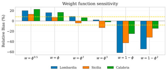
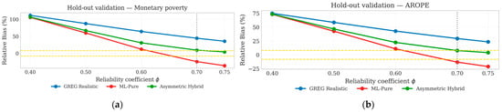
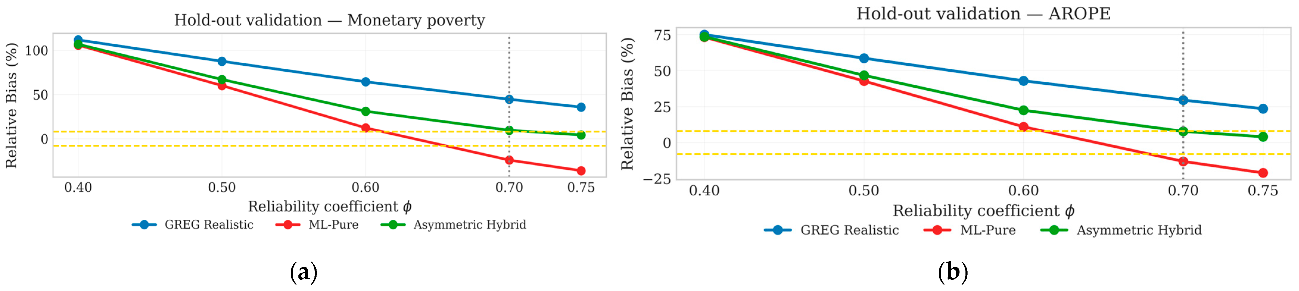
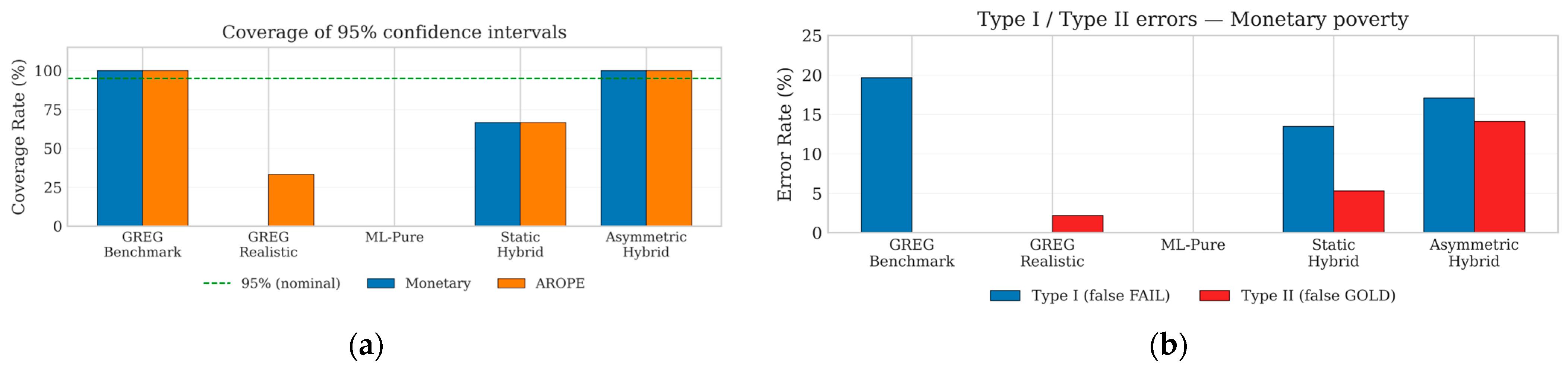

Disclaimer/Publisher’s Note: The statements, opinions and data contained in all publications are solely those of the individual author(s) and contributor(s) and not of MDPI and/or the editor(s). MDPI and/or the editor(s) disclaim responsibility for any injury to people or property resulting from any ideas, methods, instructions or products referred to in the content. |
© 2026 by the author. Licensee MDPI, Basel, Switzerland. This article is an open access article distributed under the terms and conditions of the Creative Commons Attribution (CC BY) license.