Grünwald–Letnikov Fractional Ensemble with α-Specific Power Weighting for Multi-Cancer Classification

Abstract

Standard ensemble classifiers assign weights based on performance over a single feature space, leaving multi-scale fractional representations unexplored as a tabular augmentation strategy. This study proposes the FRAE (Fractional-order Recalibrated Adaptive Ensemble) framework, which applies Grünwald–Letnikov (GL) derivatives at four memory orders as tabular feature augmentation and couples each view’s memory order to its ensemble weight via an α-specific power exponent. FRAE was evaluated on three open-access cancer datasets—WAW-TACE HCC (n = 198), Ye Prostate Cancer (C1 n = 298; C2 n = 300, external), and HANCOCK HNSCC (n = 763)—against nine baselines under 5-fold stratified cross-validation, with ablation across ten configurations. FRAE ranks first by MCC in D2 (0.587 vs. CAWPE 0.563) and second in D1 and D3, with the highest sensitivity in D3 (0.766). Ablation confirms that GL feature augmentation, not weight allocation, is the primary performance driver, contributing a directionally consistent AUC increment of 0.82–1.41 percentage points across all three tasks. On the external cohort, FRAE achieves AUC = 0.8305 [95% CI: 0.7772, 0.8739], ranking first by F1 and NPV, and tied for first by MCC among ten models, though confidence intervals overlap across all model pairs. Multi-institutional prospective validation remains the necessary next step.

1. Introduction

Cancer remains one of the leading causes of morbidity and mortality worldwide, with close to 20 million new cases and 9.7 million deaths globally in 2022 [1]. Three cancer types addressed in this study represent heterogeneous clinical decision problems suitable for evaluating generalizable predictive analytics frameworks: hepatocellular carcinoma (HCC)—the predominant form of primary liver cancer, accounting for 75–85% of cases, with a high mortality-to-incidence ratio reflecting late-stage diagnosis [2]; prostate cancer—the second most frequently diagnosed cancer and fifth leading cause of cancer death among men worldwide [3]; and head and neck squamous cell carcinoma (HNSCC)—the seventh most common cancer diagnosis globally, with approximately 890,000 new cases and 450,000 deaths annually [4].

Accurate clinical decision support for these malignancies relies on the ability to classify patients from heterogeneous tabular features—including radiomics descriptors, laboratory biomarkers, and hematological ratios—which vary substantially in distribution, scale, and predictive signal across cancer sites. Ensemble learning methods reduce variance and bias through model combination, with classifier diversity identified as the principal driver of generalization over single classifiers [5,6]. Empirical support for this advantage in tabular medical data includes applications to pancreatic cancer [7] and multi-omics cancer classification [8]. However, standard ensemble weighting schemes such as CAWPE assign weights by raising cross-validated performance estimates to a fixed power exponent applied to a single feature space [9]; weights therefore reflect predictive accuracy but not the information content of the underlying representation.

Fractional calculus—the generalization of differentiation and integration to non-integer orders—has attracted growing interest as a feature engineering and optimization tool in machine learning (ML) [10]. The Grünwald–Letnikov (GL) and Caputo definitions of the fractional derivative are the most widely implemented in discrete computational settings. By parameterizing the derivative order α ∈ (0, 1), fractional operators interpolate between pure memory (α → 0, integrating the entire history of the signal) and the integer-order first difference (α → 1, capturing only local change). This memory intensity spectrum has been applied in biomedical signal modeling; for example, as a feature operator in image-based cancer detection [11] and as a physiological parameter in cardiovascular biomarker modeling [12].

In the ML literature, fractional operators have been incorporated primarily at the optimizer level: Wu et al. [13] proposed the fractional light gradient boosting machine (NFLightGBM), in which a non-causal fractional difference operator—defined as half the difference of causal and anti-causal fractional difference operators via Z-transform—replaces the integer-order gradient descent step within LightGBM, reporting performance improvements on eight benchmark datasets. A parallel development applied a fractional gradient descent algorithm to extreme gradient boosting [14]. In both approaches, the fractional operator is applied at the gradient update step during model training; the input feature space remains integer-ordered and unmodified. This application point differs from the present work, in which GL fractional derivatives are applied directly as feature transformation operators on tabular clinical data—constructing augmented feature views prior to ensemble learning rather than modifying the optimization trajectory within a single learner. Herrera-Alcántara [15] demonstrated Caputo-derivative-based gradient optimizers for neural network training in human activity recognition, and Raubitzek et al. [10] reviewed the full landscape of fractional-derivative integration in ML, noting that the use of fractional operators as feature space transformation tools for tabular clinical data remains underexplored. To the best of the author’s knowledge, no prior work has applied GL derivatives simultaneously as a tabular feature augmentation operator within a multi-cancer validated ensemble framework.

Ensemble methods—including gradient boosting, random forests, stacking, and weighted probabilistic combination—have been widely applied to cancer classification from tabular clinical and biomarker data. For HCC and TACE response prediction, radiomics-based random survival forest and XGBoost models have been shown to complement clinical Cox regression models in prognostic tasks [16,17]. For prostate cancer diagnosis, automated ML pipelines combining PSA variants and routine complete blood count (CBC) parameters have achieved improved specificity over PSA screening alone [18]. For HNSCC, a deep neural network with recursive feature elimination trained on systemic inflammatory markers demonstrated competitive post-treatment recurrence detection with external validation on an independent institutional cohort [19]. Despite these advances, each study validates a single model architecture on a single cancer cohort; cross-cancer generalizability and fractional-order feature transformation remain unaddressed in this literature.

A structured comparison of representative studies published in 2023–2026, evaluating each study across five key analytical dimensions—feature type, method category, multi-dataset validation, use of fractional feature transformation, and use of fractional ensemble weighting—is presented in Table 1.

Table 1. Comparison of selected studies (2023–2026) on fractional calculus in ML and ensemble methods for cancer classification.

Study	Cancer/Task	Feature	Method	MD	FF	FW	Key Metric/Limitation
[13]	Generic benchmarks (incl. breast cancer)	Tabular	NFLightGBM (fractional difference in optimizer step)	Y	N	N	Acc = 0.993/fractional in optimizer only; no cancer clinical context
[11]	Melanoma (HAM10000; 7-class)	Image	GL + EfficientNetV2S	N	Y	N	Acc = 0.810; F1 = 0.81/no tabular; no ensemble; no MCC
[20]	Breast cancer	Tabular	7 ML classifiers + Caputo ODE	N	N	N	Acc = 0.977; AUC = 0.995/fractional in ODE only; no ensemble weighting
[21]	Tumor (benign vs. malignant; n = 608)	Tabular	FrFT + BP neural network	N	Y	N	Acc = 0.932/no AUC/MCC
[22]	Brain tumor MRI (4-class)	Image	GL denoising + ResNet50–EfficientNetB0	Y	Y	N	Acc = 0.988/GL in image denoising only
[23]	32 cancer types (TCGA)	Tabular (genomic)	Single XGBoost	N	N	N	BACC = 77.53%; AUC = 0.97/no ensemble weighting
[24]	Colorectal cancer + liver metastasis	Tabular	AdaBoost	N	N	N	Acc = 0.911/private data; no AUC; no MCC
[25]	Lung cancer (2 datasets)	Tabular	Hard voting (RF + SVM + LR)	Y	N	N	Acc = 99%/92.5%/no AUC; no MCC
[26]	Breast cancer (WDBC)	Tabular	Stacking ensemble	N	N	N	Acc = 0.999/no MCC; no external validation
[18]	Prostate cancer	Tabular	AutoML (H2O GBM)	N	N	N	AUC = 0.72/private data; no external validation; no MCC
[27]	Prostate cancer (n = 84)	Tabular + image	Stacking ensemble (TabPFN + LightGBM + EfficientNetV2)	N	N	N	F1 = 0.907; AUC = 0.911/no MCC; private data
[19]	HNSCC (n = 778 + n = 173 ext.)	Tabular	DNN-RFE	Y	N	N	AUC = 0.883 (CV); 0.784 (ext.)/no ensemble weighting; no MCC
[28]	Breast cancer (WDBC)	Tabular	Stacking + DL meta-learner	N	N	N	Acc = 0.977; AUC = 0.974/no external validation; no MCC
[16]	HCC (TACE outcome) (n = 252)	Radiomics	Random survival forest	N	N	N	C-index = 0.713/No external validation
[17]	HCC post-TACE (n = 105)	Radiomics + tabular	XGBoost	N	N	N	AUC = 0.979 (train), 0.750 (test)/severe imbalance; no external validation
[7]	Pancreatic cancer	Tabular	Soft voting (RF + NB)	N	N	N	AUC = 0.990/no MCC; uniform voting weights
This Study	HCC, PCa, HNSCC	Tabular	FRAE: GL multi-view + α-specific weighting	Y	Y	Y	AUC = 0.8305, MCC = 0.5846 (both external, C2, n = 300)/same-institution external validation

Note: MD = multi-dataset validation; FF = fractional feature transformation; FW = fractional ensemble weighting; Y = yes; and N = no.

Across these studies, none simultaneously applies GL fractional feature transformation, AUC-based ensemble recalibration, and multi-cancer validation with an external holdout cohort—a gap that motivates three open problems. First, current ensemble methods for clinical tabular classification do not exploit the memory structure of feature spaces: weights assigned to ensemble components reflect predictive performance but not the transformation scale or information depth of the underlying feature representation. Second, AUC alone is an insufficient primary evaluation criterion for imbalanced clinical classification tasks: it does not account for the cost asymmetry between false positives and false negatives [29], and under a class imbalance its optimistic bias—arising from the inflated true-negative denominator of FPR—can obscure Poor minority class performance [30]; deployment-sensitive metrics that integrate sensitivity, calibration, and discriminative capacity under different clinical priorities are needed. Third, existing fractional calculus ML methods confine the fractional operator to the gradient update step rather than to the input feature space, leaving tabular GL feature augmentation across multiple cancer datasets unexplored.

To address these gaps, this study proposes Fractional-order Recalibrated Adaptive Ensemble (FRAE), a multi-view ensemble framework that simultaneously applies GL fractional derivatives as a tabular feature augmentation operator and couples the fractional order of each view to its AUC-based ensemble weight.

The specific contributions are as follows:

(i)

GL fractional derivatives at four orders (α ∈ {0.3, 0.5, 0.7, 0.9}) are applied row-wise to the tabular feature matrix, constructing complementary augmented views whose correlation structure with the original feature space varies systematically because the binomial coefficient decay rate varies with α.

(ii)

Each view’s ensemble weight is coupled to its GL memory order via an α-specific power exponent, producing dataset-adaptive, non-uniform weight distributions. This constitutes a structural contribution: the ablation study confirms that the mechanism produces non-degenerate weight distributions but does not confer a measurable AUC advantage over uniform weighting—indicating that view diversity, not weight allocation, is the primary performance driver.

(iii)

The framework is evaluated across three heterogeneous cancer tasks—HCC, prostate cancer, and HNSCC—spanning different feature types, imbalance ratios, and sample sizes, with a fully held-out external cohort (n = 300) evaluated under a lock-and-test protocol.

Together, these contributions establish a computationally reproducible fractional-order ensemble framework for multi-cancer classification, evaluated with an initial external validation assessment under a lock-and-test protocol.

2. Materials and Methods

2.1. Datasets

Three publicly available cancer datasets were used. Each involves a binary classification task with a clinically defined outcome and heterogeneous tabular features. Dataset characteristics—including sample size, feature count, imbalance ratio (IR), and preprocessing configuration—are summarized in Table 2.

Table 2. Dataset characteristics.

ID	Name	Cancer Type	Task	n	Raw Features	Selected	IR	Positive Class
D1	WAW-TACE [31]	Hepatocellular carcinoma	TACE response	198	549 (clinical + radiomics)	20 (MI top 20)	1.00	TACE responder
D2	Ye Prostate [32]	Prostate cancer	Diagnosis	298 (C1 train) + 300 (C2 ext)	18 (clinical lab)	18 (all)	1.24 (C1)/1.40 (C2)	Cancer-positive
D3	HANCOCK [33]	HNSCC	Overall survival	763	53 (clinical + pathological + blood + derived)	53 (all)	2.58	Deceased

2.1.1. D1—WAW-TACE

The WAW-TACE dataset comprises 198 patients with HCC who underwent transarterial chemoembolization (TACE) at a single center. The classification task is TACE response prediction (responder vs. non-responder). The raw feature space contains 549 variables combining pre-treatment clinical measurements and CT-based radiomics descriptors extracted using PyRadiomics [34]. The survival time variable was excluded before feature selection to prevent outcome leakage, and the top 20 features were selected by mutual information with the binary outcome. The class distribution is balanced (n_pos = 99, n_neg = 99; IR = 1.00).

2.1.2. D2—Ye Prostate

The Ye Prostate Cancer dataset was partitioned into two independent cohorts: a Training-and-Validation Cohort (C1; n = 298; 133 cancer-positive, 165 cancer-negative; IR = 1.24) and an External Validation Cohort (C2; n = 300; 125 cancer-positive, 175 cancer-negative; IR = 1.40). The task is prostate cancer diagnosis (cancer-positive vs. cancer-negative). The feature space consists of 18 clinical laboratory markers including prostate-specific antigen (PSA) variants (tPSA, fPSA, PSAD, and prostate volume), CBC parameters, and demographic variables; all 18 features were retained. The observed class distributions differ slightly from the Mendeley repository descriptions (C1: 131 positive, 167 negative; C2: 127 positive, and 173 negative); this discrepancy originates in the repository metadata and does not reflect any record exclusion during preprocessing.

2.1.3. D3—HANCOCK

The HANCOCK dataset comprises 763 patients with HNSCC. The task is overall survival prediction, operationalized as a binary outcome (deceased vs. living). Multi-modal features were constructed from three source files: clinical records, pathological reports, and pre-treatment blood panel analytes. Clinical records included age, year of diagnosis, days to first treatment, sex, smoking status, and metastasis status; pathological reports provided positive and resected lymph node counts, resection margin, infiltration depth, pT stage, and histological grade; and blood analytes comprised 38 measurements covering CBC, coagulation, and biochemistry markers, each extracted as the patient’s earliest pre-treatment value. Three derived hematological ratios were additionally computed: neutrophil-to-lymphocyte ratio (NLR = granulocytes/lymphocytes), platelet-to-lymphocyte ratio (PLR = platelets/lymphocytes), and lymphocyte-to-monocyte ratio (LMR = lymphocytes/monocytes). The final feature matrix contains 53 variables, all retained without further selection. The dataset is imbalanced (n_pos = 213, n_neg = 550; IR = 2.58), which is consistent with the class distribution in the original data release.

2.1.4. Preprocessing

For all three datasets, missing and infinite values were replaced by column-wise medians (SimpleImputer, strategy = ‘median’), with imputation parameters fitted exclusively on training folds. Features were then standardized using QuantileTransformer (output_distribution = ‘normal’, random_state = 42), which maps each feature marginal to an approximate standard normal distribution. A secondary StandardScaler was applied within each per-view feature space as part of the GL view construction process described below. All preprocessing steps were fitted on the training partition of each CV fold and applied to the corresponding validation partition without refitting, ensuring no information leakage across folds.

2.2. Grünwald–Letnikov Fractional Derivative

The GL definition of the fractional derivative is employed as the feature transformation operator. For a discrete sequence x = {x₀, x₁, …, x_N−1} and fractional order α ∈ (0, 1), the GL derivative of order α at position n is defined in Equation (1) as [35,36]:

$$D_n^{\left(\alpha \right)}\left[x\right]={\displaystyle \sum _{k=0}^n{c}_k}{x}_{n-k}$$

(1)

where the binomial-type coefficients $c_k$ satisfy the recursion in Equation (2):

$$c_0=1, c_k=c_{k-1}\cdot {\displaystyle \frac{k-1-\alpha }{k}}, k=1,2,\dots ,n$$

(2)

The GL formulation admits a direct discrete implementation on finite sequences without numerical integration, making it computationally tractable for tabular clinical data. This distinguishes it from the Riemann–Liouville and Caputo definitions, which require convolution integrals over continuous domains [36].

For α ∈ (0, 1), the coefficients $c_k$ are non-zero for all k ≤ n, rendering $D^{\left(\alpha \right)}$ a non-local operator in which each transformed value incorporates contributions from all preceding observations. The decay rate of $\left|c_k\right|$ with increasing lag k increases with α, which is consistent with the theoretical properties of the GL operator. Consequently, lower α values weight distant observations more heavily—approaching a cumulative weighted sum of all preceding features—while higher α values approach the behavior of the integer-order first difference (α → 1). This memory intensity spectrum motivates the multi-view design of FRAE: each GL order captures a different transformation scale of the feature space, contributing complementary discriminative information to the ensemble.

The GL operator is applied row-wise to each patient’s feature vector, treating the feature index as a surrogate sequential dimension rather than a temporal one. Each transformed value at position n encodes a weighted sum of preceding features with binomial-coefficient-decaying weights, producing augmented views whose correlation structure with the original feature space varies with α. Column ordering follows the data loading and preprocessing sequence, was held constant across all folds and models, and its sensitivity was evaluated via a 10-permutation test. Four values α ∈ {0.3, 0.5, 0.7, 0.9} were selected to provide approximately uniform coverage of (0, 1), excluding the boundary values α = 0 (constant transform) and α = 1 (integer-order first difference). These values were fixed a priori without dataset-specific tuning; sensitivity to this grid choice was assessed using three alternative grids: Grid A {0.2, 0.4, 0.6, 0.8}, Grid B {0.1, 0.3, 0.5, 0.7}, and Grid C {0.4, 0.6, 0.8, 0.95}.

2.3. FRAE Framework

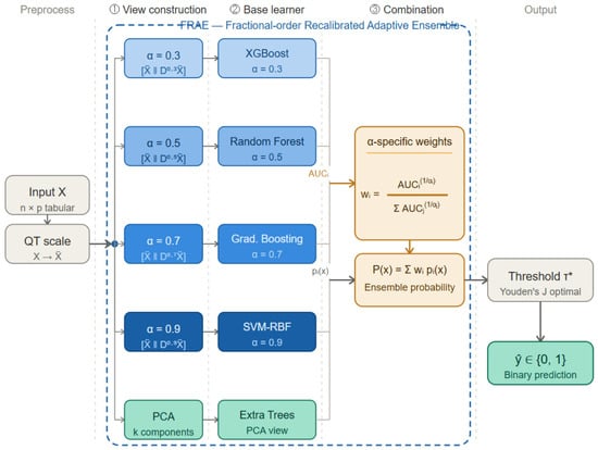
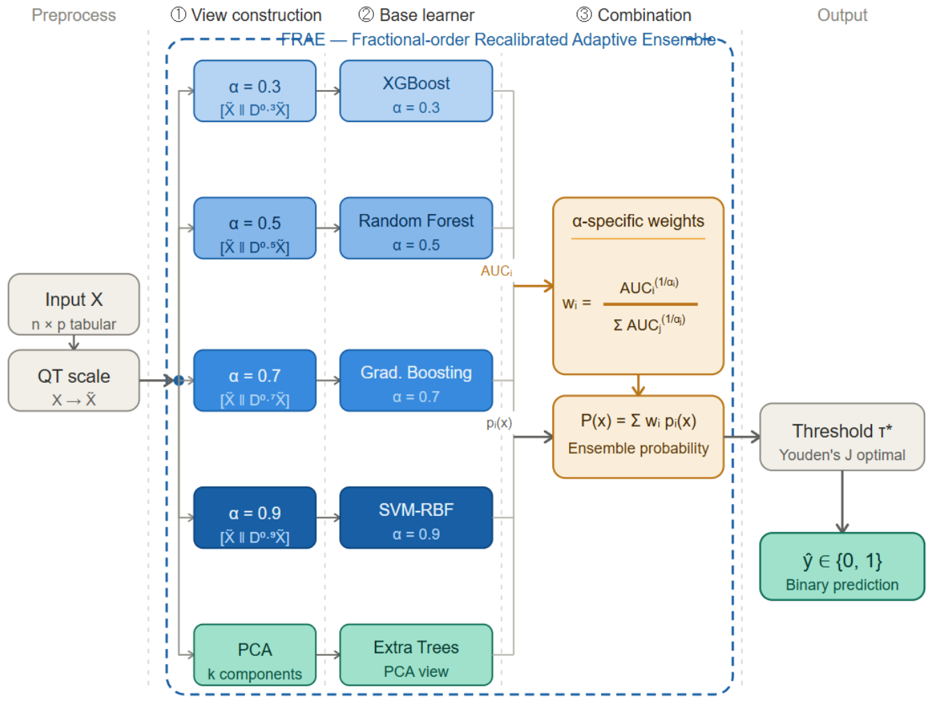
The FRAE framework combines GL fractional derivative feature views with an α-specific fractional power ensemble weighting mechanism. As shown in Figure 1, the FRAE pipeline proceeds through three core stages.

Figure 1. FRAE architecture (dashed border). Blue gradient encodes GL memory order: light (α = 0.3, long memory) → dark (α = 0.9, near-integer derivative). Learner box colors match the corresponding GL view. AUC_i feeds α-specific weight computation; p_i(x) feeds ensemble probability aggregation. Binary prediction ŷ is obtained via Youden’s J-optimal threshold τ*. Preprocessing (QT scale) is applied prior to the three core FRAE stages.

2.3.1. View Construction Stage

Five parallel feature views are constructed from the QT-scaled input matrix X ∈ ℝ^n×p. For each α_i ∈ {0.3, 0.5, 0.7, 0.9}, the GL derivative is computed row-wise and horizontally concatenated with the original features to form the augmented view matrix V_i = [X ‖ D^(α_i⁾X] ∈ ℝ^{n×2p}, which is subsequently standardized using StandardScaler fitted on the training fold. The fifth view is obtained by applying PCA to X to extract k orthogonal components, where k = 8 for D1 and D2 and k = 10 for D3; the PCA transform is fitted on the training fold only. The four GL views capture memory-weighted feature interactions at different scales, while the PCA view provides a decorrelated linear summary of the original feature space.

2.3.2. Base Learners

Each view is processed by a dedicated base learner with a fixed assignment: XGBoost (α = 0.3 view), random forest (RF) (α = 0.5 view), gradient boosting (GB) (α = 0.7 view), Support Vector Machine with RBF kernel (SVM-RBF) (α = 0.9 view), and Extra Trees (ETs) (PCA view). Architectural diversity across classifier families—gradient-boosted trees, kernel methods, and randomized ensemble classifiers—is maintained by design, as classifier diversity has been identified as a driver of ensemble generalization [5,6]. Each base learner yields a per-fold area under the ROC curve (AUC) value, AUC_i ∈ [0, 1], and a class-probability vector p_i(x). All base learner hyperparameters are fixed a priori without tuning; complete configurations are listed in Table A1.

2.3.3. α-Specific Fractional Power Weighting

The ensemble weight assigned to view i is defined in Equation (3) as:

$$w_i={\displaystyle \frac{{\mathrm{AUC}}_i^{1/{\alpha }_i}}{{\displaystyle \sum _{j=1}^5{\mathrm{AUC}}_j^{1/{\alpha }_j}}}}$$

(3)

where α_i ∈ {0.3, 0.5, 0.7, 0.9} for the four GL views. The weights satisfy w_i ≥ 0 and Σ_iw_i = 1. The exponent 1/α_i controls weight sensitivity to AUC differences: lower α yields a larger exponent, amplifying inter-view performance differences relative to higher α views. Weights are estimated on the training partition of each fold and applied to the corresponding validation partition to prevent leakage.

The PCA view was assigned a fractional exponent of α = 0.5, which is a conventional midpoint of the unit interval; sensitivity to this assignment was assessed across α_PCA ∈ {0.1, 0.3, 0.5, 0.7, 0.9}.

This formulation differs structurally from CAWPE [9], as summarized in Table 3. The term adaptive in FRAE refers to dataset-specific weights computed from cross-validated AUC performance via α-specific power exponents—not to iterative weight updates during training—and the fractional exponent 1/α_i constitutes the principal structural distinction from CAWPE.

Table 3. Structural comparison of FRAE and CAWPE ensemble weighting mechanisms.

Property	CAWPE	FRAE
Weight formula	wi = AUCiα/Σj AUCjα (α = 4)	wi = AUCi(1/αi)/Σj AUCj(1/αj)
Exponent type	Fixed power exponent (α = 4)	Fractional: 1/αi, view-specific
α-order dependence	None	αi ∈ {0.3, 0.5, 0.7, 0.9} per GL view; α = 0.5 (PCA)
Memory encoding	None	αi encodes GL memory intensity
Feature space	Single (QT-scaled X)	Five views: 4 × [XQT ‖ D(αi) XQT] + 1 × PCA(XQT)
Base learners	5 (XGBoost, RF, GB, SVM-RBF, ETs)—matched to FRAE	5 (XGBoost, RF, GB, SVM-RBF, ETs); one per view
Weight amplification	Power (α = 4): amplifies differences in 5-fold cross-validated AUC estimates (re-implementation; original uses 10-fold cross-validated accuracy)	Fractional power: magnitude controlled by 1/αi
Decision threshold	Youden’s J (τ*) (re-implementation; original uses argmax probability)	Youden’s J (τ*)

2.3.4. Ensemble Aggregation and Threshold Optimization

The ensemble probability for an observation x is computed in Equation (4) as the weighted mean of per-view estimates:

$$P\left(x\right)={\displaystyle \sum _{i=1}^5{w}_i{p}_i}\left(x\right)$$

(4)

The binary prediction ŷ is obtained in Equation (5) by applying a dataset-specific threshold τ*:

$$\widehat{y}=1\left[P(x)\ge {\tau }^{\ast }\right]$$

(5)

The threshold τ* is determined by Youden’s J criterion [37], defined in Equation (6):

$${\tau }^{\ast }=\underset{\tau \in \left[0,1\right]}{\arg \max }J\left(\tau \right), J\left(\tau \right)=\mathrm{Sensitivity}\left(\tau \right)+\mathrm{Specificity}\left(\tau \right)-1$$

(6)

τ* is estimated on the training partition of each fold and applied to the corresponding validation partition. Youden’s J criterion was selected because it jointly optimizes sensitivity and specificity without requiring prior specification of a cost ratio between false positives and false negatives [38].

2.4. Baseline Models

Nine baseline classifiers were evaluated: Logistic Regression (LR), linear-kernel SVM (SVM-Lin), SVM-RBF, RF, ETs, GB, Multilayer Perceptron (MLP), XGBoost, and CAWPE. All single classifiers receive the same QT-scaled feature space (QuantileTransformer-scaled, with mutual information selection applied only to D1). CAWPE is re-implemented following the power exponent weighting scheme of Large et al. [9]—w_i ∝ p_i^α (α = 4)—using five base classifiers (XGBoost, RF, GB, SVM-RBF, and ETs), which are identical to the FRAE base learner set, operating on the same QT-scaled feature space without GL views (Table 3). Three modifications from the original formulation were adopted: (1) fold-level AUC replaces cross-validated accuracy as the performance estimate p_i; (2) Youden’s J-optimal threshold replaces the original argmax-probability decision rule; and (3) 5-fold stratified CV replaces the original 10-fold CV. Class imbalance was addressed using class_weight = ‘balanced’ for LR, SVM-Lin, SVM-RBF, RF, ETs, and MLP. All hyperparameters are fixed a priori without tuning; complete configurations for all nine baselines are listed in Table A2.

2.5. Evaluation Metrics

Classification performance was assessed using AUC, F1-score, Matthews correlation coefficient (MCC), sensitivity, specificity, positive predictive value (PPV), negative predictive value (NPV), and accuracy. MCC was prioritized as the primary summary metric because it incorporates all four cells of the confusion matrix and is more informative than F1 and accuracy under class imbalance [29]; it is defined in Equation (7) as:

$$\mathrm{MCC}={\displaystyle \frac{\mathrm{TP}\cdot \mathrm{TN}-\mathrm{FP}\cdot \mathrm{FN}}{\sqrt{\left(\mathrm{TP}+\mathrm{FP}\right)\left(\mathrm{TP}+\mathrm{FN}\right)\left(\mathrm{TN}+\mathrm{FP}\right)\left(\mathrm{TN}+\mathrm{FN}\right)}}}$$

(7)

where TP, TN, FP, and FN denote true positives, true negatives, false positives, and false negatives, respectively. AUC, F1, MCC, sensitivity, and specificity were computed as means across five CV folds; accuracy is reported as the fold mean with standard deviation and 95% Wald confidence interval (CI; mean ± 1.96 × SD/√5). The Expected Calibration Error (ECE) [39] and Brier score [40] were additionally computed to characterize probability calibration. The area under the precision–recall curve (average precision, AP) was computed as a supplementary calibration-related metric under class imbalance, complementing AUC where the positive class is underrepresented [30]. For probability calibration assessment, ECE, Brier score, AUC, and MCC are additionally computed on pooled out-of-fold predictions; pooled and fold mean values are reported alongside each other where they differ.

Pairwise comparisons between FRAE and each baseline were conducted using a two-sided paired t-test on fold-level accuracy values (n = 5 pairs per comparison), with effect size quantified by Cohen’s d. These comparisons are exploratory; inference is based on directional consistency and effect size magnitudes. p-values are reported without correction for multiple comparisons, which is consistent with the exploratory framing; effect sizes (Cohen’s d) are reported alongside p-values as the primary measure of practical difference magnitude [41]. The significance levels used throughout were ns = p > 0.05, * = p ≤ 0.05, ** = p ≤ 0.01, and *** = p ≤ 0.001. Post hoc calibration was assessed using Platt scaling and isotonic regression within a nested 4-fold inner CV.

To address concerns regarding the sensitivity of the Grünwald–Letnikov derivative to the arbitrary ordering of input features, a column permutation test was conducted for each dataset. Ten independent random permutations of the feature columns were applied prior to FRAE evaluation (random seeds 0–9), and AUC and MCC were recorded for each permutation. The standard deviation and range of the resulting AUC distribution serve as a robustness index: a small SD (<0.01) indicates that FRAE performance is not substantially driven by the order in which features are presented to the GL operator.

2.6. Feature Importance and Correlation Analysis

Feature importance was assessed per dataset using an RF classifier (n_estimators = 300, class_weight = ‘balanced’, random_state = 42) on the preprocessed feature space. Three importance criteria were computed: RF impurity-based importance, absolute Pearson correlation |r| between each feature and the binary outcome, and mean absolute SHAP values (described below). A consensus rank was defined as the mean of each feature’s rank under these three criteria (RF importance, |r|, and SHAP), with lower mean rank indicating higher importance. SHAP (SHapley Additive exPlanations) values were additionally computed using TreeExplainer [42] for the RF classifier to provide model-specific feature attribution scores.

To examine whether GL-derived features introduce information beyond the original feature space, the Pearson cross-correlation matrix between original features and their GL-transformed counterparts was computed for D2 (first 12 of 18 features shown; 12 × 12 matrix) at each α ∈ {0.3, 0.5, 0.7, 0.9}. The diagonal of this matrix captures same-feature self-correlation between original and transformed versions, while off-diagonal entries quantify cross-feature information.

2.7. Ablation Study

To quantify the contribution of individual FRAE components, an ablation study was conducted over ten model configurations. The baseline is the full FRAE with all four GL views (α ∈ {0.3, 0.5, 0.7, 0.9}), the PCA view, and α-specific fractional power weighting. Nine ablated variants were constructed by systematically removing individual views (without α = 0.3, without α = 0.5, without α = 0.7, without α = 0.9, and without PCA), replacing fractional power weights with uniform weights (w_i = 0.2 for all i), removing all GL features while retaining the PCA view (no-fractional: PCA-only view processed by ETs, without any GL augmentation), retaining only the α = 0.9 view (single-view α = 0.9), and retaining only the α = 0.7 and α = 0.9 views (two-view α = 0.7 + 0.9). All ablated variants use the same preprocessing, CV protocol, and threshold optimization as the full FRAE.

2.8. External Validation Protocol

Consistent with the original dataset design, C1 (n = 298) is used exclusively for model training and 5-fold stratified CV, and C2 (n = 300) is reserved as a fully held-out External Validation Cohort [32]. No hyperparameter selection, threshold tuning, or any form of model fitting was performed using C2 data at any stage of development. The Youden’s J-optimal threshold and fractional power ensemble weights were determined exclusively from C1 cross-validation and applied without modification to C2.

Bootstrap confidence intervals (n = 1000 stratified resamples with replacement, random_state = 42) were computed for AUC, F1, MCC, sensitivity, and specificity on the external cohort C2; PPV, NPV, and Youden’s J are reported as point estimates.

2.9. Experimental Setup

All experiments were implemented in Python 3.10 with scikit-learn 1.6.1, XGBoost 1.7.x, NumPy 1.26.4, and Pandas 2.2.3. Experiments were conducted on an Intel Core i7-4770 processor (3.40 GHz, 4 cores) with 16 GB RAM running Windows 10. A 5-fold stratified CV (StratifiedKFold, n_splits = 5, shuffle = True, random_state = 42) was applied uniformly across all models and datasets, preserving the positive-class proportion in each fold. The GL derivative was implemented using the recursive coefficient formula without reliance on any external fractional calculus library, ensuring computational reproducibility. Decision thresholds were swept over τ ∈ [0.25, 0.55] in increments of 0.05.

3. Results

3.1. Classification Performance

Table 4 reports the AUC, F1, MCC, sensitivity, specificity, and accuracy (mean ± SD across 5 folds) for all 10 models across three datasets under 5-fold stratified CV. FRAE achieves the highest F1 and MCC in D2 and the highest sensitivity in D3; in D1, CAWPE achieves the highest sensitivity (0.790) and highest F1 (0.717) and MCC (0.404), while FRAE leads by specificity (0.625) and ranks second by MCC (0.384).

Table 4. Classification performance under 5-fold stratified CV.

Model	Accuracy ± SD	Sensitivity	Specificity	F1	AUC	MCC
D1 WAW-TACE (HCC, n = 198, IR = 1.00)
LR	0.6111 ± 0.0704	0.6061	0.6162	0.5912	0.6432	0.2223
SVM-Lin	0.5957 ± 0.0633	0.5960	0.5959	0.5780	0.6290	0.1919
SVM-RBF	0.4808 ± 0.0617	0.4040	0.5556	0.4127	0.4953	−0.0408
RF	0.6061 ± 0.0544	0.6162	0.5960	0.5936	0.6397	0.2124
ETs	0.5908 ± 0.0652	0.5960	0.5858	0.5751	0.6015	0.1819
GB	0.6012 ± 0.0473	0.6061	0.5960	0.5848	0.6506	0.2022
MLP	0.5353 ± 0.0389	0.5253	0.5454	0.5137	0.5991	0.0707
XGBoost	0.5908 ± 0.0537	0.5960	0.5858	0.5740	0.6699 (†)	0.1818
CAWPE	0.6867 ± 0.0554 (†)	0.7895 (†)	0.5879	0.7166 (†)	0.6682	0.4044 (†)
FRAE	0.6817 ± 0.0573	0.7368	0.6253 (†)	0.6948	0.6652	0.3837
D2 Ye Prostate (C1, n = 298, IR = 1.24)
LR	0.7315 ± 0.0322	0.7077	0.7515	0.6999	0.7297	0.4725
SVM-Lin	0.7449 ± 0.0179	0.6464	0.8242	0.6917	0.7330	0.4890
SVM-RBF	0.7182 ± 0.0151	0.6915	0.7394	0.6808	0.7332	0.4412
RF	0.7687 ± 0.0402	0.6630	0.8545	0.7180	0.7672	0.5366
ETs	0.7653 ± 0.0302	0.6553	0.8545	0.7115	0.7740	0.5324
GB	0.7385 ± 0.0433	0.7225 (†)	0.7515	0.7109	0.7439	0.4793
MLP	0.7246 ± 0.0550	0.6789	0.7636	0.6870	0.7338	0.4759
XGBoost	0.7688 ± 0.0371	0.7080	0.8182	0.7286	0.7791	0.5376
CAWPE	0.7821 ± 0.0336	0.7080	0.8424	0.7411	0.7939 (†)	0.5627
FRAE	0.7921 ± 0.0317 (†)	0.6860	0.8788 (†)	0.7435 (†)	0.7910	0.5867 (†)
D3 HANCOCK (HNSCC, n = 763, IR = 2.58)
LR	0.6829 ± 0.0498	0.6255	0.7055	0.5225	0.7238	0.3047
SVM-Lin	0.7261 ± 0.0031	0.0423	0.9909 (†)	0.0784	0.7244	0.1189
SVM-RBF	0.7326 ± 0.0187	0.1548	0.9564	0.2381	0.6954	0.1915
RF	0.7051 ± 0.0126	0.0707	0.9509	0.1155	0.7102	0.0488
ETs	0.7392 ± 0.0151 (†)	0.1316	0.9745	0.2162	0.7105	0.2151
GB	0.7157 ± 0.0382	0.2875	0.8818	0.3531	0.7048	0.2000
MLP	0.6698 ± 0.0253	0.3719	0.7855	0.3791	0.6056	0.1585
XGBoost	0.7222 ± 0.0261	0.2966	0.8873	0.3703	0.7041	0.2218
CAWPE	0.6960 ± 0.0489	0.7234	0.6855	0.5711 (†)	0.7331 (†)	0.3736 (†)
FRAE	0.6579 ± 0.0480	0.7662 (†)	0.6164	0.5561	0.7224	0.3468

Note: (†) Best value per column within each dataset. Accuracy: fold mean ± SD across 5 folds; 95% CI = mean ± 1.96 × (SD/√5). Sensitivity, specificity, F1, AUC, and MCC: fold mean. All models use Youden’s J-optimal threshold τ*.

In D1 (WAW-TACE, n = 198), FRAE attains sensitivity = 0.7368, specificity = 0.6253 (†), F1 = 0.6948, MCC = 0.3837, and AUC = 0.6652 (accuracy 0.6817 ± 0.0573, 95% CI [0.631, 0.732]). CAWPE achieves the highest F1 (0.7166 (†)) and MCC (0.4044 (†)), with accuracy indistinguishable from FRAE (0.6867 ± 0.0554 (†) vs. 0.6817 ± 0.0573). For the AUC, FRAE ranks second behind XGBoost (0.6699), differing by 0.0047. All models cluster within an AUC range of 0.495–0.670, reflecting the difficulty of radiomics-based TACE response prediction.

In D2 (Ye Prostate, C1, n = 298), FRAE achieves the highest F1 (0.7435 (†)), MCC (0.5867 (†)), accuracy (0.7921 (†) ± 0.0317, 95% CI [0.764, 0.820]), and specificity (0.8788 (†)); GB attains the highest sensitivity (0.7225 (†)). CAWPE attains the highest AUC (0.7939 (†)), marginally exceeding FRAE (0.7910; Δ = 0.0029).

In D3 (HANCOCK, n = 763, IR = 2.58), FRAE attains AUC = 0.7224, MCC = 0.3468, F1 = 0.5561, sensitivity = 0.7662 (†), and accuracy = 0.6579 ± 0.0480 at τ* = 0.25. CAWPE ranks first by AUC (0.7331 (†)), MCC (0.3736 (†)), and F1 (0.5711 (†)), and ETs ranks first by accuracy (0.7392 (†)); FRAE ranks fourth by AUC and second by MCC and F1. Models operating at high specificity thresholds—such as SVM-Lin (accuracy = 0.726, sensitivity = 0.042)—identify almost no positive cases despite higher overall accuracy, illustrating the sensitivity–specificity trade-off at IR = 2.58.

3.2. Statistical Significance

Table 5 reports pairwise comparisons between FRAE and each baseline model using a two-sided paired t-test on fold-level accuracy. Given only five fold-level observations per comparison, these tests are underpowered; the results indicate the direction of the effect rather than confirmatory evidence.

Table 5. Pairwise accuracy comparisons between FRAE and baseline models.

Comparison	Δ Accuracy	t-Statistic	p-Value	Significance	Cohen’s d
D1 WAW-TACE
FRAE vs. LR	+0.0705	2.396	0.0987	ns	0.860
FRAE vs. SVM-Lin	+0.0853	2.367	0.1017	ns	0.945
FRAE vs. SVM-RBF	+0.2009	2.366	0.1018	ns	1.723
FRAE vs. RF	+0.0756	2.973	0.0565	ns	1.043
FRAE vs. ETs	+0.0909	2.972	0.0565	ns	1.256
FRAE vs. GB	+0.0805	3.516	0.0347	*	1.800
FRAE vs. MLP	+0.1464	13.244	0.0003	***	2.793
FRAE vs. XGBoost	+0.0909	3.607	0.0226	*	1.613
FRAE vs. CAWPE	−0.0050	−0.196	0.8544	ns	−0.087
D2 Ye Prostate
FRAE vs. LR	+0.0607	2.344	0.0791	ns	1.048
FRAE vs. SVM-Lin	+0.0473	2.059	0.1086	ns	0.921
FRAE vs. SVM-RBF	+0.0740	4.226	0.0134	*	1.890
FRAE vs. RF	+0.0234	1.247	0.2804	ns	0.558
FRAE vs. ETs	+0.0268	1.971	0.1200	ns	0.882
FRAE vs. GB	+0.0537	4.021	0.0159	*	1.798
FRAE vs. MLP	+0.0676	1.633	0.1778	ns	0.730
FRAE vs. XGBoost	+0.0234	1.719	0.1607	ns	0.769
FRAE vs. CAWPE	+0.0100	1.169	0.3073	ns	0.523
D3 HANCOCK
FRAE vs. LR	−0.0250	−1.529	0.2432	ns	−0.512
FRAE vs. SVM-Lin	−0.0682	−3.139	0.0484	*	−2.007
FRAE vs. SVM-RBF	−0.0748	−4.081	0.0218	*	−2.053
FRAE vs. RF	−0.0472	−2.626	0.0786	ns	−1.347
FRAE vs. ETs	−0.0813	−3.738	0.0287	*	−2.288
FRAE vs. GB	−0.0578	−2.667	0.0755	ns	−1.333
FRAE vs. MLP	−0.0119	−0.610	0.6144	ns	−0.310
FRAE vs. XGBoost	−0.0643	−2.843	0.0638	ns	−1.666
FRAE vs. CAWPE	−0.0381	−1.559	0.1941	ns	−0.697

Note: ns = p > 0.05; * = p ≤ 0.05; and *** = p ≤ 0.001. Two-sided paired t-test on per-fold accuracy (n = 5 pairs, df = 4). Negative Δ accuracy and Cohen’s d in D3 reflect FRAE’s sensitivity-optimized threshold (τ* = 0.25).

In D1, FRAE achieves statistically significant improvement over GB (p = 0.035), XGBoost (p = 0.023), and MLP (p = 0.0003). Comparisons with the remaining six baselines—including CAWPE (p = 0.854, d = −0.087)—are non-significant, which is consistent with the near-identical fold-level accuracy of FRAE (0.6817) and CAWPE (0.6867). In D2 (C1, n = 298), statistically significant improvement is observed over two of nine baselines: SVM-RBF (p = 0.013, d = 1.890) and GB (p = 0.016, d = 1.798). Comparisons with the remaining seven baselines—including CAWPE (p = 0.307, d = 0.523) and XGBoost (p = 0.161)—are non-significant. Effect sizes remain moderate to large for LR (d = 1.048), SVM-Lin (d = 0.921), and MLP (d = 0.730). In D3, FRAE achieves significantly lower accuracy than SVM-Lin (p = 0.048, d = −2.007), SVM-RBF (p = 0.022, d = −2.053), and ETs (p = 0.029, d = −2.288), reflecting the sensitivity-oriented threshold (τ* = 0.25) that sacrifices accuracy for recall under IR = 2.58. The FRAE vs. CAWPE comparison remains non-significant (p = 0.194, d = −0.697).

3.3. α-Specific Weight Analysis

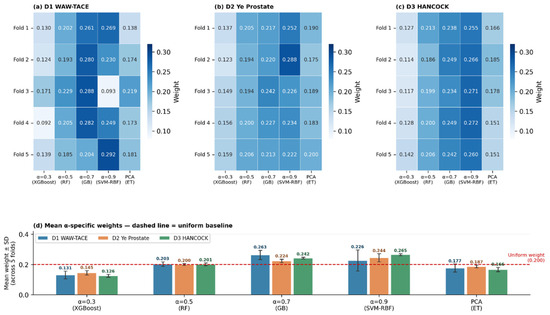
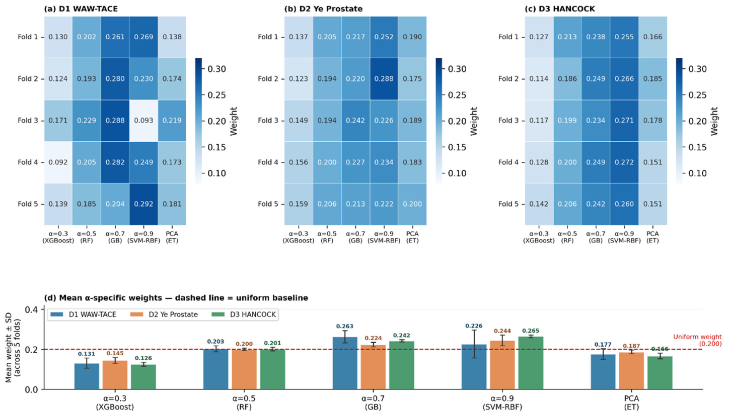
Figure 2 presents the α-specific fractional power weights as heatmaps (rows = folds, columns = views); Table 6 provides the numerical summary. The heatmaps reveal that α = 0.7 receives the highest mean weight in D1 (0.263 ± 0.031), while α = 0.9 dominates in D2 (0.244 ± 0.027) and D3 (0.265 ± 0.007). Fold-to-fold SD is highest for the α = 0.9 view in D1 (SD = 0.070) and lowest for the α = 0.5 view across all datasets (SD = 0.015 in D1, 0.006 in D2, and 0.009 in D3).

Figure 2. α-specific fractional power weight heatmaps and mean ± SD across folds.

Table 6. α-specific fractional power weights (mean ± SD across 5 folds).

Dataset	α = 0.3 (XGBoost)	α = 0.5 (RF)	α = 0.7 (GB)	α = 0.9 (SVM-RBF)	PCA (ETs)	Max/Min
D1 WAW-TACE	0.1311 ± 0.0256	0.2028 ± 0.0149	0.2630 ± 0.0307	0.2264 ± 0.0697	0.1768 ± 0.0261	2.01×
D2 Ye Prostate (C1, n = 298)	0.1448 ± 0.0146	0.1997 ± 0.0060	0.2238 ± 0.0111	0.2444 ± 0.0269	0.1872 ± 0.0091	1.69×
D3 HANCOCK	0.1256 ± 0.0098	0.2010 ± 0.0089	0.2423 ± 0.0059	0.2648 ± 0.0066	0.1663 ± 0.0140	2.11×

Note: Max/Min = ratio of highest to lowest mean weight. All weights sum to 1.00 per fold.

3.4. Feature Importance and GL Feature Correlation Analysis

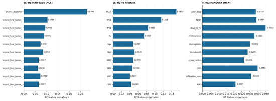
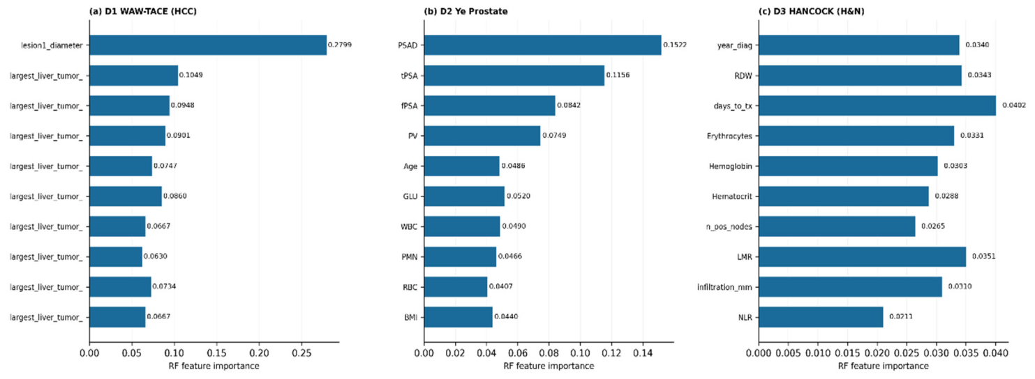
Figure 3 presents the top 10 features by consensus rank (RF importance, |Pearson r|, and SHAP) for each dataset; complete rankings with all three scores are in Table A3. Bar lengths represent RF importance, the primary component of the consensus rank.

Figure 3. Top 10 features by consensus rank (RF importance, |r|, SHAP) for D1, D2, and D3.

In D1 (WAW-TACE), lesion1_diameter dominates (RF = 0.280, |r| = 0.260, SHAP = 0.091), accounting for more than twice the importance of the second-ranked feature (GLCM-MCC: RF = 0.105, SHAP = 0.048). All top 10 features are radiomics-derived (GLCM, GLSZM, GLRLM, GLDM, and ngtdm descriptors), with no clinical or demographic variables appearing in the top tier.

In D2 (Ye Prostate), the top four features are all PSA-domain markers—PSAD (RF = 0.152, |r| = 0.200, SHAP = 0.107), tPSA (RF = 0.116, |r| = 0.217, SHAP = 0.062), fPSA (RF = 0.084, |r| = 0.222, SHAP = 0.042), and PV (RF = 0.075, |r| = 0.167, SHAP = 0.042)—collectively accounting for 43% of the total RF importance. The remaining top 10 features (ranked 5th–10th by consensus Rank_c) include Age (5th; Rank_c = 6.33, RF = 0.049), GLU (6th; Rank_c = 8.33, RF = 0.052), WBC (7th; Rank_c = 8.67, RF = 0.049), PMN (8th; Rank_c = 9.33, RF = 0.047), RBC (9th; Rank_c = 9.67, RF = 0.041), and BMI (10th; Rank_c = 10.67, RF = 0.044).

In D3 (HANCOCK), year_diag ranks first by |r| (0.207, RF = 0.034, SHAP = 0.022), followed by RDW (rank 2; RF = 0.034, |r| = 0.175, SHAP = 0.024) and days_to_tx (rank 3; RF = 0.040, |r| = 0.133, SHAP = 0.024). Erythrocyte-related markers occupy ranks 4–6 (erythrocytes: |r| = 0.196; hemoglobin: |r| = 0.180; and hematocrit: |r| = 0.178). The LMR (lymphocyte-to-monocyte ratio) ranks 8th by SHAP (0.025) despite a low |r| (0.072), suggesting the nonlinear predictive value was not captured by correlation. n_pos_nodes (rank 7) and NLR (rank 10) complete the top 10, highlighting that both hematological status and pathological staging variables contribute to survival prediction in this HNSCC cohort.

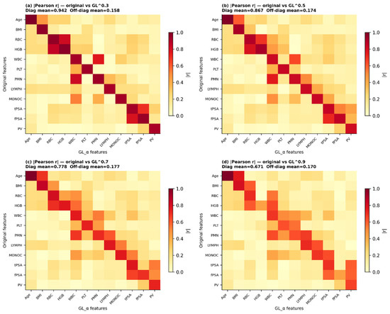
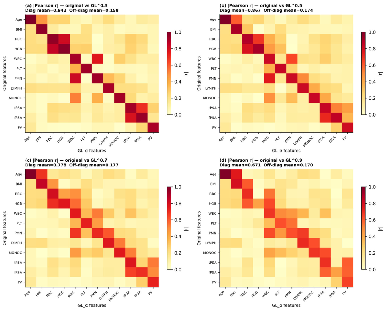
Figure 4 presents the absolute Pearson correlation |r| between original and GL-transformed features at each α for D2 C1 (n = 298), showing the first 12 features. Each panel is a 12 × 12 matrix: rows are original features, columns are GL-transformed features at the same α.

Figure 4. Absolute Pearson correlation |r| between original and GL-transformed features (D2, first 12 features).

Diagonal entries (same-feature self-correlation, |r| of orig_X vs. GL_X) decrease monotonically with increasing α: mean |r| = 0.942 (α = 0.3; diagonal-to-off-diagonal ratio = 5.95×), 0.867 (α = 0.5; ratio = 4.99×), 0.778 (α = 0.7; ratio = 4.40×), and 0.671 (α = 0.9; ratio = 3.94×), confirming that higher GL orders impose progressively stronger transformations on the original feature space. The off-diagonal mean |r| remains low across all four panels (0.158, 0.174, 0.177, and 0.170 at α = 0.3, 0.5, 0.7, 0.9, respectively), indicating that the GL operator does not introduce spurious cross-feature dependencies.

At α = 0.3, Age shows perfect self-correlation (|r| = 1.000), which persists across all four panels, indicating that the GL operator at all tested orders preserves the Age feature almost entirely. This is consistent with the mathematical behavior of the GL operator on slowly varying or constant-rate sequences: for a feature with near-zero variance across the ordered index, the memory-weighted sum converges to a value highly correlated with the original, regardless of α. At α = 0.9, the features with the lowest self-correlation are HGB (|r| = 0.429) and fPSA (|r| = 0.435), indicating that the near-integer derivative most substantially transforms these two biomarkers relative to others.

Notably, high off-diagonal values are observed specifically for biologically correlated feature pairs: orig_RBC vs. GL_HGB (|r| = 0.817 at α = 0.3) and orig_HGB vs. GL_RBC (|r| = 0.855 at α = 0.3) reflect the known co-variation between red blood cell count and hemoglobin concentration. Similarly, orig_WBC vs. GL_PMN reaches |r| = 0.761 at α = 0.3, which is consistent with the fact that PMN (polymorphonuclear neutrophils) is a major component of the WBC count. These cross-feature correlations diminish with increasing α, as the stronger transformation breaks the linear dependency.

3.5. Ablation Study and Sensitivity Analysis

3.5.1. Component Ablation

Table 7 reports the mean AUC per configuration per dataset across ten ablated variants. The no-fractional variant—retaining the PCA-only view processed by Extra Trees, without any GL augmentation—degrades AUC consistently across all three datasets (D1: −1.04%, D2: −0.82%, and D3: −1.41%), indicating that GL feature augmentation contributes positively regardless of feature space dimensionality.

Table 7. Ablation study results.

Configuration	D1		D2		D3
	AUC	ΔAUC	AUC	ΔAUC	AUC	ΔAUC
Full FRAE	0.6652	—	0.7910	—	0.7224	—
Without α = 0.3	0.6749	+0.97%	0.7869	−0.41%	0.7335	+1.12%
Without α = 0.5	0.6784	+1.32%	0.7858	−0.52%	0.7337	+1.13%
Without α = 0.7	0.6759	+1.07%	0.7855	−0.55%	0.7338	+1.15%
Without α = 0.9	0.6779	+1.27%	0.7847	−0.63%	0.7286	+0.62%
Without PCA	0.6717	+0.65%	0.7912	+0.02%	0.7228	+0.05%
Uniform weights	0.6662	+0.11%	0.7906	−0.04%	0.7209	−0.14%
No-fractional (PCA + ETs only)	0.6547	−1.04%	0.7828	−0.82%	0.7082	−1.41%
Single-view α = 0.9	0.6798	+1.46%	0.7828	−0.82%	0.7158	−0.66%
Two-view α = 0.7 + 0.9	0.6758	+1.06%	0.7913	+0.03%	0.7256	+0.32%

Note: ΔAUC = (AUC_config − AUC_Full FRAE) × 100 percentage points. AUC reported as the fold mean across 5 folds.

Replacing the α-specific fractional power weights with uniform weights (w_i = 0.2 for all i) produces near-zero AUC changes across all three datasets (ΔAUC: +0.11%, −0.04%, and −0.14%), indicating that multi-view feature construction is the primary performance driver and that the weighting mechanism does not confer a measurable AUC advantage over uniform weighting in this experimental setting. The mechanism is nonetheless non-degenerate, producing non-uniform weight distributions across all three datasets (Table 6). The single-view ablation (α = 0.9 only) degrades AUC in D2 by 0.82% (to 0.7828), matching the no-fractional variant. In D1 (n = 198), individual view removals yield modest AUC gains (+0.65–+1.32%). This pattern is consistent with the bias-variance trade-off in small-sample settings. Each individual GL view may introduce variance that exceeds its marginal information gain; the ensemble collectively retains discriminative value that is lost only when all views are removed simultaneously (ΔAUC = −1.04%). In D2 (n = 298), individual view removals consistently degrade AUC (−0.41% to −0.63%), while in D3 (n = 763), individual removals yield modest gains (+0.62% to +1.15%), a pattern similar to D1 that may reflect the higher imbalance (IR = 2.58) and the Youden’s J threshold constraint at τ* = 0.25.

3.5.2. Sensitivity to Pre-Specified Choices

Three configuration choices were fixed a priori without tuning: the column ordering supplied to the row-wise GL operator, the fractional-order grid α ∈ {0.3, 0.5, 0.7, 0.9}, and the exponent α = 0.5 assigned to the PCA view for weighting. Each was assessed separately.

Column permutation analysis (Table A4) indicates that FRAE performance is stable under feature reordering. Across 10 permutations per dataset, AUC standard deviations were 0.0045 (D1), 0.0020 (D2), and 0.0026 (D3), with total ranges of 0.014, 0.007, and 0.009. Permuted MCC exceeded the original ordering in D1 and D3, indicating that the loading-sequence ordering is not privileged. Stability under permutation confirms that FRAE performance is not driven by the specific feature ordering, though this test cannot distinguish the contribution of binomial decay weighting from that of any fixed linear feature mixing.

Three alternative grids were evaluated: Grid A {0.2, 0.4, 0.6, 0.8}, Grid B {0.1, 0.3, 0.5, 0.7}, and Grid C {0.4, 0.6, 0.8, 0.95} (Table A5). AUC deviations from the original grid ranged from −0.92 to +0.51 pp (D1), −0.31 to +0.09 pp (D2), and +0.62 to +0.83 pp (D3). MCC was more responsive than AUC, with deviations from −4.70 pp (D1, Grid B) to +2.10 pp (D3, Grid A). Grid C, which emphasizes higher fractional orders, produced non-negative AUC deviations in all three datasets, which is consistent with the pattern that higher α values receive greater ensemble weighting in D2 and D3. Grid B, which extends to α = 0.1, produced the largest degradation in D1 and D2, indicating that long-memory orders contribute least under the present configuration.

Sensitivity analysis across α_PCA ∈ {0.1, 0.3, 0.5, 0.7, 0.9} yielded AUC ranges of 0.0085 (D1), 0.0034 (D2), and 0.0013 (D3)—at least an order of magnitude below the between-model AUC spread within each dataset (Table 4). This assignment is therefore not a material determinant of performance.

3.6. ROC Analysis and Threshold Sensitivity

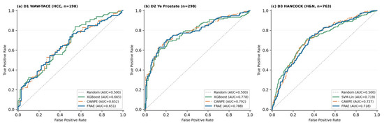
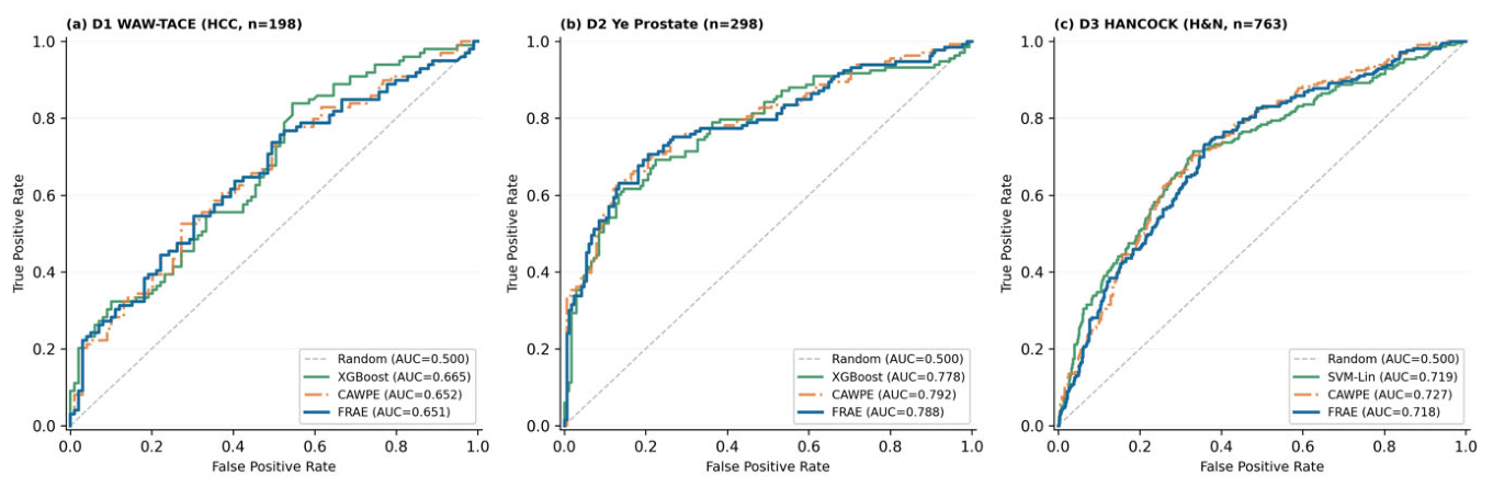
Figure 5 presents ROC curves for FRAE, CAWPE, and the best single baseline classifier per dataset (pooled 5-fold predictions). In D1, FRAE and CAWPE achieve near-identical pooled AUC (0.651 vs. 0.652), with XGBoost being the highest at 0.665. In D2 (C1, n = 298), CAWPE pooled AUC = 0.792 marginally exceeds FRAE (0.788) and XGBoost (0.778)—a difference consistent with the non-significant pairwise accuracy test (Table 5). In D3, CAWPE pooled AUC = 0.727 exceeds FRAE (0.718) and SVM-Lin (0.719). Pooled values (concatenated fold predictions) differ from the fold mean values in Table 4 due to between-fold aggregation; this applies to both AUC (D1: 0.651 vs. 0.665; D2: 0.788 vs. 0.791; and D3: 0.718 vs. 0.722) and Youden’s J (D1: 0.233 vs. 0.362; D2: 0.559 vs. 0.565; and D3: 0.336 vs. 0.383; the fold mean values from Table A6).

Figure 5. ROC curves for FRAE, CAWPE, and the best single baseline classifier per dataset.

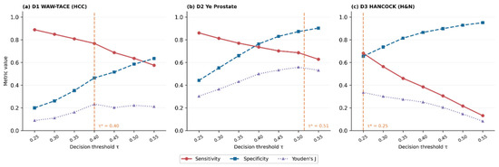
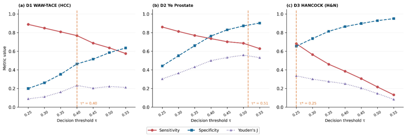
Figure 6 presents the threshold sensitivity analysis across τ ∈ [0.25, 0.55]. Youden’s J-optimal thresholds (pooled predictions across folds): τ* = 0.40 (D1, J = 0.233), τ* = 0.5143 (D2, J = 0.559), and τ* = 0.25 (D3, J = 0.336). At τ* = 0.5143 in D2, FRAE achieves sensitivity = 0.686 and specificity = 0.873. At τ* = 0.25 in D3, sensitivity = 0.682 and specificity = 0.655, declining monotonically thereafter as τ increases.

Figure 6. Threshold sensitivity analysis τ ∈ [0.25, 0.55] with Youden’s J-optimal τ per dataset.

3.7. Probability Calibration and Platt Scaling

Table 8 reports the AUC, MCC, ECE, and Brier score before and after Platt scaling and isotonic regression; both calibrators were applied within a nested 4-fold inner CV. ECE and Brier score are computed on pooled out-of-fold predictions. The fold mean ECE for all ten models is reported in Table A7 for consistency with all other CV metrics in this paper. Pooled ECE is lower than the fold mean ECE because fold-specific calibration deviations partially cancel when predictions are concatenated across folds—a property of the bin-averaging estimator that is well-characterized in the calibration literature.

Table 8. Effect of post hoc calibration on FRAE probability reliability.

Dataset	Condition	AUC	MCC	ECE	Brier	Cal. Quality
D1 WAW-TACE	Uncalibrated	0.6652	0.3972	0.101	0.2414	Poor
	Platt scaling	0.6652 (†)	0.3972 (†)	0.054	0.2376	Acceptable
	Isotonic reg.	0.6403	0.3176	0.084	0.2434	Acceptable
D2 Ye Prostate	Uncalibrated	0.7910	0.5867	0.066	0.1803	Acceptable
	Platt scaling	0.7910 (†)	0.5867 (†)	0.064	0.1805	Acceptable
	Isotonic reg.	0.7870	0.5130	0.054	0.1845	Acceptable
D3 HANCOCK	Uncalibrated	0.7178	0.3491	0.034	0.1786	Acceptable
	Platt scaling	0.7178 (†)	0.3491 (†)	0.030	0.1797	Acceptable
	Isotonic reg.	0.7184	0.3327	0.024	0.1791	Acceptable

Note: Calibration quality: ECE < 0.10 = Acceptable; ECE ≥ 0.10 = Poor. ECE and Brier score computed on pooled out-of-fold predictions. (†) Reported to confirm rank invariance under calibration.

The AUC and MCC invariances documented in Table 8 constrain their own interpretation: they confirm that Platt scaling preserves rank-based discrimination, but provide no evidence regarding the reliability of probability estimates as absolute risk statements.

3.8. External Validation on D2 Cohort 2

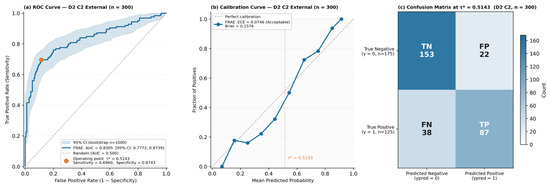
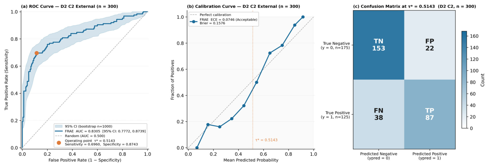
FRAE was trained on C1 (n = 298) and evaluated on the held-out C2 external cohort (n = 300; 125 cancer-positive, 175 cancer-negative; IR = 1.40) with τ* = 0.5143 and ensemble weights fixed from C1 cross-validation. Figure 7 presents a three-panel external validation summary for FRAE on C2 (n = 300). Figure 7 shows the ROC curve (AUC = 0.8305 [95% CI: 0.7772, 0.8739]); the bootstrap confidence band confirms stable performance across all FPR values, with the operating point at τ* = 0.5143 yielding sensitivity = 0.696 and specificity = 0.874. Figure 7b shows the calibration curve (ECE = 0.0746, Acceptable), with mild overconfidence at predicted probabilities of 0.25–0.55 and slight underconfidence above 0.65; Brier score = 0.1576. Figure 7c shows the confusion matrix at τ* = 0.5143: TN = 153, FP = 22, FN = 38, TP = 87; PPV = 0.798 and NPV = 0.801. Complete discrimination and calibration metrics for all 10 models are provided in Table 9; clinical safety metrics including PPV, NPV, Youden’s J, and confusion matrix elements are provided in Table A8.

Figure 7. External validation of FRAE on D2 C2 (n = 300). (a) ROC curve. (b) Calibration curve. (c) Confusion matrix at τ*.

Table 9. External validation—discrimination and calibration metrics for all 10 models on D2 cohort 2.

Model	AUC [95% CI]	F1 [95% CI]	MCC [95% CI]	Sensitivity [95% CI]	Specificity [95% CI]	ECE	Brier
FRAE	0.8305 [0.7772, 0.8739]	0.7436 (†) [0.6782, 0.8031]	0.5846 (†) [0.4903, 0.6755]	0.6960 [0.6154, 0.7752]	0.8743 [0.8212, 0.9231]	0.0746	0.1576
RF	0.8251 [0.7714, 0.8763]	0.7234 [0.6578, 0.7833]	0.5495 [0.4564, 0.6427]	0.6800 [0.5967, 0.7607]	0.8571 [0.8057, 0.9064]	0.1011	0.1654
ETs	0.8237 [0.7734, 0.8755]	0.7414 [0.6759, 0.8034]	0.5846 (†) [0.4947, 0.6783]	0.6880 [0.6071, 0.7721]	0.8800 [0.8297, 0.9286]	0.1021	0.1621
CAWPE	0.8346 (†) [0.7798, 0.8819]	0.7382 [0.6727, 0.7964]	0.5775 [0.4824, 0.6667]	0.6880 [0.6016, 0.7656]	0.8743 [0.8225, 0.9198]	0.0791	0.1538 (†)
GB	0.8182 [0.7675, 0.8668]	0.6923 [0.6295, 0.7535]	0.4587 [0.3602, 0.5624]	0.7200 (†) [0.6429, 0.8000]	0.7429 [0.6823, 0.8078]	0.1195	0.1771
XGBoost	0.8108 [0.7597, 0.8593]	0.6888 [0.6201, 0.7566]	0.4813 [0.3785, 0.5820]	0.6640 [0.5757, 0.7482]	0.8114 [0.7500, 0.8721]	0.0915	0.1706
SVM-Lin	0.7407 [0.6810, 0.7953]	0.6201 [0.5472, 0.6864]	0.3931 [0.2884, 0.4913]	0.5680 [0.4848, 0.6480]	0.8114 [0.7500, 0.8663]	0.0899	0.1976
SVM-RBF	0.7393 [0.6796, 0.7939]	0.6320 [0.5616, 0.6986]	0.3691 [0.2661, 0.4732]	0.6320 [0.5538, 0.7143]	0.7371 [0.6666, 0.8011]	0.0498 (†)	0.1988
LR	0.7387 [0.6784, 0.7959]	0.6104 [0.5339, 0.6822]	0.3341 [0.2223, 0.4423]	0.6080 [0.5159, 0.6977]	0.7257 [0.6648, 0.7882]	0.0854	0.1970
MLP	0.7238 [0.6627, 0.7809]	0.6250 [0.5504, 0.6882]	0.3465 [0.2377, 0.4428]	0.6400 [0.5504, 0.7154]	0.7086 [0.6375, 0.7742]	0.2370	0.2637

Note: (†) denotes the best value per column.

On C2, bootstrap confidence intervals overlap across all model pairs; the rankings reported below quantify estimation patterns in this single external cohort (n = 300) rather than establish statistical superiority. Within these constraints, FRAE attains the highest F1 (0.744 (†)), MCC (0.585 (†), tied with ETs), PPV (0.798 (†)), NPV (0.801 (†)), and Youden’s J (0.570 (†)). CAWPE attains the highest AUC (0.8346 (†)) and lowest Brier score (0.1538 (†)); GB attains the highest sensitivity (0.720 (†)) and TP count (90 (†)); ETs attains the highest TN (154 (†)) and lowest FP (21 (†)); and SVM-RBF attains the lowest ECE (0.050 (†)).

4. Discussion

4.1. Principal Findings

FRAE attains the highest F1 and MCC in D2, and the highest sensitivity in D3, under a unified hyperparameter configuration. In D1 and D3, CAWPE achieves higher F1 and MCC, reflecting the performance advantage of ensemble combination on a single feature space for those datasets. Sensitivity is highest in D1 (0.737) and D3 (0.766); in D2, where prostate cancer class imbalance is moderate (IR = 1.24), the sensitivity-maximizing model is GB (0.723), while FRAE achieves 0.686 at a threshold that jointly optimizes sensitivity and specificity.

MCC is used as the primary performance criterion throughout. By MCC, FRAE ranks first in D2 (0.587 vs. CAWPE 0.563) and second in D1 (0.384 vs. CAWPE 0.404) and D3 (0.347 vs. CAWPE 0.374). By AUC—a threshold-independent metric—FRAE ranks second in D1 and D2 (behind XGBoost and CAWPE respectively), and fourth in D3. In D2, CAWPE attains a marginally higher AUC than FRAE (0.7939 vs. 0.7910; Δ = 0.0029), while FRAE attains higher MCC (0.587 vs. 0.563) and F1 (0.744 vs. 0.741); the difference is non-significant (Table 5), reflecting the comparable overall performance of the two base learner-matched ensemble architectures on this clinical laboratory dataset.

Because FRAE and CAWPE differ simultaneously in feature space, weighting formula, and base learner composition (Table 3), the observed performance difference reflects the combined effect of all three dimensions. CAWPE should therefore be interpreted as an alternative ensemble architecture rather than a controlled comparator for the weighting mechanism in isolation.

These patterns suggest that GL feature augmentation provides its greatest marginal gain when the original feature space has limited discriminative range—in D2, the AUC range across all ten models is 0.064—or when balanced metric performance is prioritized over the raw AUC rank.

4.2. Ablation Study and Role of GL Features

The ablation results provide evidence for the contribution of each FRAE component. The consistent AUC degradation under the no-fractional variant (D1: −1.04%, D2: −0.82%, D3: −1.41%) aligns with the low off-diagonal correlation (0.158–0.177) between original and GL-transformed features, supporting the interpretation that GL features introduce information not collinear with the original feature space.

The near-zero AUC change under uniform weighting (Table 7; ΔAUC: +0.11%, −0.04%, and −0.14% across D1, D2, and D3) indicates that view diversity, not weight allocation, is the primary performance driver. The α-specific mechanism nonetheless produces structured, non-uniform weight distributions without additional hyperparameter search, constituting a cost-free structural component even when its AUC contribution is negligible. The single-view ablation (α = 0.9 only) matches the no-fractional variant in D2, which is consistent with the interpretation that view diversity rather than any individual view’s discriminative strength is the primary driver of gain. Individual GL view removals produce modest AUC changes across datasets (D1: +0.65% to +1.32%; D2: −0.41% to −0.63%; and D3: +0.62% to +1.15%), which is consistent with the principle that each view contributes a small marginal increment when others are present [6]. The PCA view contributes negligibly in D2 (Without PCA ΔAUC = +0.02%), indicating that a decorrelated linear summary adds little beyond the GL views in compact clinical laboratory feature spaces. Marginal PCA contributions are observed in D1 (+0.65%) and D3 (+0.05%), which is consistent with greater redundancy-reduction potential at higher feature dimensionality.

4.3. α-Specific Weight Patterns

The dataset-dependent weight pattern—higher α favored in D2 and D3, moderate α (=0.7) favored in D1—is recorded as an empirical observation. Mathematically, the GL fractional order α parameterizes the effective memory window through the binomial coefficient decay rate: as α → 1, the operator shrinks toward a local finite difference transform, while lower α retains longer-range weighted contributions from preceding feature indices [43]. This mathematical property is well-characterized and dataset-independent. Why specific α values receive higher ensemble weights for specific feature types—radiomics in D1 versus clinical laboratory markers in D2 and D3—cannot be causally determined in this framework. The GL operator is applied row-wise with an arbitrary column ordering, and no controlled variation in the feature order was performed. Fractional-order parameters have been interpreted as physiologically meaningful indices of memory in biomedical signal contexts [12,44], but such interpretation requires a sequentially meaningful input dimension, which tabular feature vectors do not provide. The weight patterns should therefore be regarded as dataset-adaptive empirical outcomes of the α-specific power weighting formula, not as evidence of a biologically grounded memory preference.

4.4. Calibration, Threshold Analysis, and Deployment Context

Calibration performance differs substantially across datasets. In D2 training cohort C1 (n = 298, IR = 1.24), FRAE achieves ECE = 0.066 (Acceptable), Brier score = 0.180, and average precision AP = 0.781—the highest among all evaluated models; SVM-RBF achieves the lowest ECE (0.043) and six of ten models reach Acceptable calibration (Table A7). On the external cohort C2, FRAE achieves ECE = 0.075 (Acceptable) and Brier score = 0.158. In D1, all models achieve Poor calibration under fold mean assessment (ECE ≥ 0.10), with FRAE achieving a fold mean ECE = 0.166. The generally Poor calibration in D1 may be attributable to the limited sample size (n = 198) and high-dimensional radiomics origin of the features. Overconfident probability estimates have been documented in high-capacity classifiers trained on limited data [45]; this tendency extends to ensemble methods applied in small high-dimensional radiomics settings [46]. The ECE metric is additionally sensitive to sample size in its bin-based estimation [39], which may partly explain the elevated ECE observed in D1.

Post hoc calibration was evaluated using Platt scaling and isotonic regression within a nested cross-validation framework. On pooled out-of-fold predictions, Platt scaling reduced the D1 ECE from 0.101 (Poor) to 0.054 (Acceptable), indicating that the D1 calibration deficit is attributable to the ensemble probability scale and is correctable by a monotone calibration layer rather than reflecting an irreducible property of the feature space. The corresponding fold mean ECE reduction is 0.166 → 0.137, which remains Poor, which is consistent with the small-sample constraint documented above. In D2 and D3, where uncalibrated ECE was already Acceptable, Platt scaling produced marginal further improvement (D2: 0.066 → 0.064; D3: 0.034 → 0.030). Isotonic regression yielded similar ECE reductions in some folds but consistently reduced MCC relative to uncalibrated FRAE (D1: 0.397 → 0.318; D2: 0.587 → 0.513), which is consistent with the known overfitting behavior of isotonic regression when calibration fold sizes are small (D1 inner validation fold: approximately 30 samples). Platt scaling is therefore recommended as the post hoc calibration step for clinical deployment of FRAE, particularly in small-sample radiomics settings.

FRAE achieves the highest Youden’s J in D2 (0.565; Table A6), reflecting the most balanced sensitivity–specificity trade-off in that dataset. In D1, CAWPE achieves the highest Youden’s J (0.377 vs. FRAE 0.362), which is consistent with CAWPE’s higher sensitivity (0.790 vs. FRAE 0.737); in D3, CAWPE similarly leads by Youden’s J (0.409 vs. FRAE 0.383) at the sensitivity-optimizing threshold. A sensitivity of 0.766 means that 23.4% of deceased patients in D3 are not flagged at τ* = 0.25. Whether this miss rate is Acceptable depends on the downstream consequence of a missed positive. For an initial screening stage where positive predictions trigger further workup, the high NPV (0.874) supports a rule-out strategy: patients classified as surviving have a high probability of truly surviving, reducing unnecessary follow-up burden.

4.5. Limitations and External Validation

Four principal limitations of the present study warrant consideration. First, the D2 External Validation Cohort (C2; n = 300) originates from the same institutional source as the training cohort (C1; n = 298) and does not constitute fully independent, multi-institutional validation. The AUC improvement observed on C2 (0.830) relative to C1 cross-validation (0.791) may partly reflect cohort-level differences in class distribution and patient composition. True generalizability—including the stability of Platt scaling calibration benefits under distribution shift—requires prospective evaluation on cohorts from independent institutions. Second, statistical comparisons are conducted on n = 5 fold-level observations, which limits power. The reported significance levels should be interpreted as exploratory and consistent-direction evidence rather than confirmatory inference; results for D2 in particular (2 of 9 comparisons are significant) reflect both the reduced power of 5-fold paired t-tests and the genuinely competitive performance of ensemble baselines on this dataset. Larger-scale replication with independent cohorts is needed. Third, three design choices were fixed a priori without optimization: the row-wise GL feature ordering (assessed via column permutation), the α grid {0.3, 0.5, 0.7, 0.9}, and the PCA view exponent (α = 0.5). XGBoost was additionally configured without class-weight reweighting, unlike other classifiers; this asymmetry is most relevant in D3 (IR = 2.58), where Youden’s J-optimal thresholding provides implicit imbalance correction. Fourth, FRAE was not benchmarked against tabular deep learning architectures such as TabNet [47], FT-Transformer [48], and SAINT [49]. The present study focuses on interpretable fractional-order ensemble mechanisms under a fixed hyperparameter configuration, where the contribution of GL feature augmentation can be isolated through ablation.

Despite these limitations, the external validation on C2 provides an initial—if institutionally constrained—generalizability assessment. The consistency between C1 cross-validation and C2 external performance (fold mean Youden’s J: 0.565 vs. 0.570; ECE: 0.066 vs. 0.075) indicates that threshold and weight transfer from C1 to C2 did not result in meaningful performance degradation, supporting the stability of the lock-and-test protocol under same-institution conditions. PPV = 0.798 and NPV = 0.801 on C2 indicate clinically useful discriminative capacity for both classes at the locked threshold, pending validation on larger independent cohorts.

5. Conclusions

GL fractional derivatives applied at multiple memory orders contribute a consistent within-framework AUC increment across three heterogeneous cancer classification tasks—HCC, prostate cancer, and HNSCC—under a single fixed hyperparameter configuration, with gains confirmed by ablation and performance profiles that vary interpretably by dataset, feature type, and evaluation metric.

Three findings warrant emphasis:

• GL feature augmentation is the primary performance driver. Removing all GL views degrades AUC by 0.82–1.41% across all three datasets; replacing α-specific weights with uniform weights changes AUC by less than 0.15%. The α-specific weighting mechanism is therefore a cost-free structural property—producing non-degenerate, dataset-adaptive weight distributions without hyperparameter search—rather than a source of discriminative gain.
• Weight adaptation is dataset-dependent and emerges without tuning. The dominant GL view shifts from α = 0.7 in D1 (radiomics) to α = 0.9 in D2 and D3 (clinical laboratory and hematological features), reflecting dataset-specific differences in view discriminability rather than a fixed design choice.
• External validation supports generalizability, with caveats. On the held-out prostate cancer cohort (n = 300), FRAE ranks first by F1 and NPV, and tied for first by MCC (with ETs), against nine baselines (AUC = 0.8305); bootstrap confidence intervals overlap across all model pairs, indicating that this cohort size does not permit unambiguous ranking.

Priority directions include multi-institutional validation across all three cancer types, data-driven GL order selection, and temperature scaling evaluation to complement the Platt scaling results reported here.

References

- Bray, F.; Laversanne, M.; Sung, H.; Ferlay, J.; Siegel, R.L.; Soerjomataram, I.; Jemal, A. Global Cancer Statistics 2022: GLOBOCAN Estimates of Incidence and Mortality Worldwide for 36 Cancers in 185 Countries. CA Cancer J. Clin. 2024, 74, 229–263. [Google Scholar] [CrossRef] [Scilit] [PubMed]
- Li, Q.; Ding, C.; Cao, M.; Yang, F.; Yan, X.; He, S.; Chen, W. Global Epidemiology of Liver Cancer 2022: An Emphasis on Geographic Disparities. Chin. Med. J. 2024, 137, 2334–2342. [Google Scholar] [CrossRef] [Scilit] [PubMed]
- Schafer, E.J.; Laversanne, M.; Sung, H.; Soerjomataram, I.; Briganti, A.; Dahut, W.; Jemal, A. Recent Patterns and Trends in Global Prostate Cancer Incidence and Mortality: An Update. Eur. Urol. 2025, 87, 302–313. [Google Scholar] [CrossRef] [Scilit] [PubMed]
- Barsouk, A.; Aluru, J.S.; Rawla, P.; Saginala, K.; Barsouk, A. Epidemiology, Risk Factors, and Prevention of Head and Neck Squamous Cell Carcinoma. Med. Sci. 2023, 11, 42. [Google Scholar] [CrossRef] [Scilit] [PubMed]
- Kuncheva, L.I.; Whitaker, C.J. Measures of Diversity in Classifier Ensembles and Their Relationship with the Ensemble Accuracy. Mach. Learn. 2003, 51, 181–207. [Google Scholar] [CrossRef] [Scilit]
- Brown, G.; Wyatt, J.; Harris, R.; Yao, X. Diversity Creation Methods: A Survey and Categorisation. Inf. Fusion 2005, 6, 5–20. [Google Scholar] [CrossRef]
- Almisned, F.A.; Usanase, N.; Ozsahin, D.U.; Ozsahin, I. Incorporation of Explainable Artificial Intelligence in Ensemble Machine Learning-Driven Pancreatic Cancer Diagnosis. Sci. Rep. 2025, 15, 14038. [Google Scholar] [CrossRef] [Scilit] [PubMed]
- Ma, B.; Meng, F.; Yan, G.; Yan, H.; Chai, B.; Song, F. Diagnostic Classification of Cancers Using Extreme Gradient Boosting Algorithm and Multi-Omics Data. Comput. Biol. Med. 2020, 121, 103761. [Google Scholar] [CrossRef] [Scilit] [PubMed]
- Large, J.; Lines, J.; Bagnall, A. A Probabilistic Classifier Ensemble Weighting Scheme Based on Cross-Validated Accuracy Estimates. Data Min. Knowl. Discov. 2019, 33, 1674–1709. [Google Scholar] [CrossRef] [Scilit] [PubMed]
- Raubitzek, S.; Mallinger, K.; Neubauer, T. Combining Fractional Derivatives and Machine Learning: A Review. Entropy 2023, 25, 35. [Google Scholar] [CrossRef] [Scilit] [PubMed]
- Anber, B.; Yurtkan, K. Fractional Differentiation Based Image Enhancement for Automatic Detection of Malignant Melanoma. BMC Med. Imaging 2024, 24, 231. [Google Scholar] [CrossRef] [Scilit] [PubMed]
- Bahloul, M.A.; Aboelkassem, Y.; Laleg-Kirati, T.M. Human Hypertension Blood Flow Model Using Fractional Calculus. Front. Physiol. 2022, 13, 838593. [Google Scholar] [CrossRef] [Scilit] [PubMed]
- Wu, H.; Mao, Y.; Weng, J.; Yu, Y.; Wang, J. Fractional Light Gradient Boosting Machine Ensemble Learning Model: A Non-Causal Fractional Difference Descent Approach. Inf. Fusion 2025, 118, 102947. [Google Scholar] [CrossRef] [Scilit]
- Wu, H.; Weng, J.; Lou, Y.; Shen, Y.; Wang, J. Fast and Accurate Fractional Order Gradient Descent Algorithm and Its Application in Extreme Gradient Boosting. Knowl.-Based Syst. 2025, 326, 114911. [Google Scholar] [CrossRef] [Scilit]
- Herrera-Alcántara, O. Fractional Derivative Gradient-Based Optimizers for Neural Networks and Human Activity Recognition. Appl. Sci. 2022, 12, 9264. [Google Scholar] [CrossRef] [Scilit]
- Bartnik, K.; Krzyziński, M.; Bartczak, T.; Korzeniowski, K.; Lamparski, K.; Wróblewski, T.; Mech, K.; Januszewicz, M.; Biecek, P. A Novel Radiomics Approach for Predicting TACE Outcomes in Hepatocellular Carcinoma Patients Using Deep Learning for Multi-Organ Segmentation. Sci. Rep. 2024, 14, 14779. [Google Scholar] [CrossRef] [Scilit] [PubMed]
- Zhang, M.; Kuang, B.; Zhang, J.; Peng, J.; Xia, H.; Feng, X.; Peng, L. Enhancing Prognostic Prediction in Hepatocellular Carcinoma Post-TACE: A Machine Learning Approach Integrating Radiomics and Clinical Features. Front. Med. 2024, 11, 1419058. [Google Scholar] [CrossRef] [Scilit] [PubMed]
- Satır, A.; Üstündağ, Y.; Yeşil, M.R.; Huysal, K. Prediction of Prostate Cancer from Routine Laboratory Markers with Automated Machine Learning. J. Clin. Lab. Anal. 2025, 39, e25143. [Google Scholar] [CrossRef] [Scilit] [PubMed]
- So, Y.K.; Kim, Z.; Cheong, T.Y.; Chung, M.J.; Baek, C.-H.; Son, Y.-I.; Seok, J.; Jung, Y.-S.; Ahn, M.-J.; Ahn, Y.C.; et al. Detection of Cancer Recurrence Using Systemic Inflammatory Markers and Machine Learning after Concurrent Chemoradiotherapy for Head and Neck Cancers. Cancers 2023, 15, 3540. [Google Scholar] [CrossRef] [Scilit] [PubMed]
- Amilo, D.; Sadri, K.; Hincal, E.; Hafez, M. A Hybrid Machine Learning and Fractional-Order Dynamical Framework for Multi-Scale Prediction of Breast Cancer Progression. CMES-Comput. Model. Eng. Sci. 2025, 145, 2189–2222. [Google Scholar] [CrossRef] [Scilit]
- Liu, X.; Gao, N.; He, S.; Wang, L. Application of Fractional Fourier Transform and BP Neural Network in Prediction of Tumor Benignity and Malignancy. Fractal Fract. 2025, 9, 267. [Google Scholar] [CrossRef] [Scilit]
- Lin, J.; Huang, L.; Ding, L.; Yan, S. Deep Brain Tumor Lesion Classification Network: A Hybrid Method Optimizing ResNet50 and EfficientNetB0 for Enhanced Feature Extraction. Fractal Fract. 2025, 9, 614. [Google Scholar] [CrossRef] [Scilit]
- Zelli, V.; Manno, A.; Compagnoni, C.; Ibraheem, R.O.; Zazzeroni, F.; Alesse, E.; Tessitore, A. Classification of Tumor Types Using XGBoost Machine Learning Model: A Vector Space Transformation of Genomic Alterations. J. Transl. Med. 2023, 21, 836. [Google Scholar] [CrossRef] [Scilit] [PubMed]
- Yu, Z.; Li, G.; Xu, W. Rapid Detection of Liver Metastasis Risk in Colorectal Cancer Patients through Blood Test Indicators. Front. Oncol. 2024, 14, 1460136. [Google Scholar] [CrossRef] [Scilit] [PubMed]
- Ali, T.M.; Mir, A.; Rehman, A.U.; Humayun, M.; Shaheen, M.; Alshammari, R.T.S. Revolutionizing Lung Cancer Detection: A High-Accuracy Machine Learning Framework for Early Diagnosis. BioMed Res. Int. 2025, 2025, 9961773. [Google Scholar] [CrossRef] [Scilit] [PubMed]
- Reshan, M.S.A.; Amin, S.; Zeb, M.A.; Sulaiman, A.; Alshahrani, H.; Azar, A.T.; Shaikh, A. Enhancing Breast Cancer Detection and Classification Using Advanced Multi-Model Features and Ensemble Machine Learning Techniques. Life 2023, 13, 2093. [Google Scholar] [CrossRef] [Scilit] [PubMed]
- El-Melegy, M.; Mamdouh, A.; Ali, S.; Badawy, M.; El-Ghar, M.A.; Alghamdi, N.S.; El-Baz, A. Prostate Cancer Diagnosis via Visual Representation of Tabular Data and Deep Transfer Learning. Bioengineering 2024, 11, 635. [Google Scholar] [CrossRef] [Scilit] [PubMed]
- Gurcan, F. Enhancing Breast Cancer Prediction through Stacking Ensemble and Deep Learning Integration. PeerJ Comput. Sci. 2025, 11, e2461. [Google Scholar] [CrossRef] [Scilit] [PubMed]
- Chicco, D.; Jurman, G. The Advantages of the Matthews Correlation Coefficient (MCC) over F1 Score and Accuracy in Binary Classification Evaluation. BMC Genom. 2020, 21, 6. [Google Scholar] [CrossRef] [Scilit] [PubMed]
- Saito, T.; Rehmsmeier, M. The Precision-Recall Plot Is More Informative Than the ROC Plot When Evaluating Binary Classifiers on Imbalanced Datasets. PLoS ONE 2015, 10, e0118432. [Google Scholar] [CrossRef] [Scilit] [PubMed]
- Bartnik, K.; Bartczak, T.; Krzyziński, M.; Korzeniowski, K.; Lamparski, K.; Węgrzyn, P.; Lam, E.; Bartkowiak, M.; Wróblewski, T.; Mech, K.; et al. WAW-TACE: A Hepatocellular Carcinoma Multiphase CT Dataset with Segmentations, Radiomics Features, and Clinical Data. Radiol. Artif. Intell. 2024, 6, e240296.2024. [Google Scholar] [CrossRef]
- Ye, H. Prostate Cancer Data, Version 1. Mendeley Data 2024. [Google Scholar] [CrossRef]
- Dörrich, M.; Balk, M.; Heusinger, T.; Beyer, S.; Mirbagheri, H.; Fischer, D.J.; Kist, A.M. A Multimodal Dataset for Precision Oncology in Head and Neck Cancer. Nat. Commun. 2025, 16, 7163. [Google Scholar] [CrossRef] [Scilit] [PubMed]
- Van Griethuysen, J.J.; Fedorov, A.; Parmar, C.; Hosny, A.; Aucoin, N.; Narayan, V.; Aerts, H.J. Computational Radiomics System to Decode the Radiographic Phenotype. Cancer Res. 2017, 77, e104–e107. [Google Scholar] [CrossRef] [Scilit] [PubMed]
- Oldham, K.; Spanier, J. The Fractional Calculus: Theory and Applications of Differentiation and Integration to Arbitrary Order; Academic Press: New York, NY, USA, 1974; Volume 111. [Google Scholar]
- Podlubny, I. Fractional Differential Equations: An Introduction to Fractional Derivatives, Fractional Differential Equations, to Methods of Their Solution and Some of Their Applications; Academic Press: San Diego, CA, USA, 1998; Volume 198. [Google Scholar]
- Youden, W.J. Index for Rating Diagnostic Tests. Cancer 1950, 3, 32–35. [Google Scholar] [CrossRef]
- Fluss, R.; Faraggi, D.; Reiser, B. Estimation of the Youden Index and Its Associated Cutoff Point. Biom. J. 2005, 47, 458–472. [Google Scholar] [CrossRef] [Scilit] [PubMed]
- Pakdaman Naeini, M.; Cooper, G.; Hauskrecht, M. Obtaining Well Calibrated Probabilities Using Bayesian Binning. In Proceedings of the AAAI Conference on Artificial Intelligence, Austin, TX, USA, 25–30 January 2015; AAAI Press: Palo Alto, CA, USA, 2015; Volume 29. [Google Scholar] [CrossRef] [Scilit]
- Brier, G.W. Verification of Forecasts Expressed in Terms of Probability. Mon. Weather Rev. 1950, 78, 1–3. [Google Scholar] [CrossRef]
- Lakens, D. Calculating and Reporting Effect Sizes to Facilitate Cumulative Science: A Practical Primer for t-Tests and ANOVAs. Front. Psychol. 2013, 4, 863. [Google Scholar] [CrossRef] [Scilit] [PubMed]
- Lundberg, S.M.; Lee, S.I. A Unified Approach to Interpreting Model Predictions. In Advances in Neural Information Processing Systems; Curran Associates: Red Hook, NY, USA, 2017; Volume 30, pp. 4765–4774. [Google Scholar]
- Abdelouahab, M.S.; Hamri, N.E. The Grünwald–Letnikov Fractional-Order Derivative with Fixed Memory Length. Mediterr. J. Math. 2016, 13, 557–572. [Google Scholar] [CrossRef] [Scilit]
- Magin, R.L. Fractional Calculus in Bioengineering. Crit. Rev. Biomed. Eng. 2004, 32, 1–104. [Google Scholar] [CrossRef] [Scilit] [PubMed]
- Guo, C.; Pleiss, G.; Sun, Y.; Weinberger, K.Q. On Calibration of Modern Neural Networks. In Proceedings of the 34th International Conference on Machine Learning, Sydney, Australia, 6–11 August 2017; PMLR: Cambridge, MA, USA, 2017; Volume 70, pp. 1321–1330. [Google Scholar]
- An, C.; Park, Y.W.; Ahn, S.S.; Han, K.; Kim, H.; Lee, S.K. Radiomics Machine Learning Study with a Small Sample Size: Single Random Training-Test Set Split May Lead to Unreliable Results. PLoS ONE 2021, 16, e0256152. [Google Scholar] [CrossRef] [Scilit] [PubMed]
- Arik, S.Ö.; Pfister, T. TabNet: Attentive Interpretable Tabular Learning. In Proceedings of the AAAI Conference on Artificial Intelligence, Virtual, 2–9 February 2021; AAAI Press: Palo Alto, CA, USA, 2021; Volume 35, pp. 6679–6687. [Google Scholar] [CrossRef] [Scilit]
- Gorishniy, Y.; Rubachev, I.; Khrulkov, V.; Babenko, A. Revisiting Deep Learning Models for Tabular Data. In Advances in Neural Information Processing Systems; Curran Associates: Red Hook, NY, USA, 2021; Volume 34, pp. 18932–18943. [Google Scholar]
- Somepalli, G.; Goldblum, M.; Schwarzschild, A.; Bruss, C.B.; Goldstein, T. SAINT: Improved Neural Networks for Tabular Data via Row Attention and Contrastive Pre-Training. arXiv 2021, arXiv:2106.01342. [Google Scholar] [CrossRef] [Scilit]
Disclaimer/Publisher’s Note: The statements, opinions and data contained in all publications are solely those of the individual author(s) and contributor(s) and not of MDPI and/or the editor(s). MDPI and/or the editor(s) disclaim responsibility for any injury to people or property resulting from any ideas, methods, instructions or products referred to in the content. |
© 2026 by the author. Licensee MDPI, Basel, Switzerland. This article is an open access article distributed under the terms and conditions of the Creative Commons Attribution (CC BY) license.