Numerical Solution of Eighth-Order Boundary Value Problem Using Shifted Horadam Collocation Method ^†

Abstract

Higher-order boundary value problems model several physical phenomena in fluid dynamics, astrophysics, hydrodynamics, beam theory, astronomy, hydromagnetic stability, and engineering. Eighth-order boundary value problems arise in the physics of various hydrodynamic stability problems, advanced structural mechanics, and several other real-world systems. This paper applies an efficient collocation method based on the shifted Horadam polynomials to obtain approximate solutions of an eighth-order boundary value problem in ordinary differential equations. The Horadam collocation method expresses the solution of the proposed problem as a shifted Horadam polynomial series. Using the zeros of the shifted Horadam polynomials as the collocation points, the proposed boundary value problem is reduced to a set of algebraic equations in the expansion coefficients of the series solution. The obtained algebraic equations are then solved for the unknown expansion coefficients using Newton’s iterative method. Two illustrative examples of the proposed boundary value problem are considered for the purpose of accuracy, efficiency, and reliability of the proposed method. Numerical solutions obtained are compared with the exact solutions and other existing solutions. Comparisons of results are demonstrated in tables and graphs. It is observed that the proposed method yields higher accuracy compared to the existing methods. This research work shows that the Horadam polynomial-based collocation method is an efficient method for obtaining accurate and reliable approximate solutions of higher-order boundary value problems in ordinary differential equations.

1. Introduction

Boundary value problems appear in several applied sciences and several other real-life phenomena such as fluid dynamics, astrophysics, hydrodynamics, beam theory, astronomy, induction motors, solid mechanics, mathematical physics, mathematical biology, economics, finance, and engineering [1]. Higher-order boundary value problems model many real-world scenarios in the aforementioned fields. As a result, a number of researchers have applied both analytical and numerical techniques to study higher-order boundary value problems [2,3,4,5,6]. To be more specific, the eighth-order boundary value problems appear in the deflection of beam theory and analysis, plate deflection theory, viscoelastic and inelastic flows, deformation of beams, and the physics of various hydrodynamic stability theories [7,8,9]. Eighth-order boundary value problems have been considered in [10] (Nonic spline method); ref. [11] (non-polynomial spline technique); ref. [12] (differential quadrature method); ref. [2] (reproducing kernel method); ref. [13,14,15] (variational iteration method); ref. [16] (modified decomposition method); ref. [17] (variational iteration decomposition); and ref. [18] (homotopy perturbation method). Recently, the authors in [3] used the Haar wavelet method to obtain numerical solutions of eighth-order boundary value problems. Moreover, very recently, Kumar et al. [8] and Raji et al. [19] used collocation methods based on Vieta–Lucas polynomials and Chebyshev polynomials to obtain numerical solutions of eighth-order boundary value problems, respectively. Others include Elahi et al. [20] (Legendre Galerkin method) and ref. [21] (Galerkin method with quintic b-spline).

In this paper, the author employs a shifted Horadam collocation method [22] to obtain numerical solutions of the eighth-order boundary value problem:

$$\begin{array}{cc}\hfill & v^{\left(8\right)}\left(x\right)=f(x,v\left(x\right),v^{\prime }\left(x\right),v^{″}\left(x\right),\dots ,v^{\left(7\right)}\left(x\right))(0<x<1)\hfill \\ \hfill & v\left(0\right)={\xi }_1,v\left(1\right)={\eta }_1,v^{\prime }\left(0\right)={\xi }_2,v^{\prime }\left(1\right)={\eta }_2,\hfill \\ \hfill & v^{″}\left(0\right)={\xi }_3,v^{″}\left(1\right)={\eta }_3,v^{‴}\left(0\right)={\xi }_4,v^{‴}\left(1\right)={\eta }_4.\hfill \end{array}$$

(1)

Since the governing problem is of the eighth order, the general solution contains eight constants of integration, which requires eight boundary conditions to obtain a unique physical state of the system. Here $v\left(x\right)$ is the deflection, displacement, or state variable, which represents the physical state of the underlying system; ${\xi }_i\in \mathbb{R}$$(i=1,2,3,4)$ are four boundary conditions specified at the start-point $x=0$, while ${\eta }_i\in \mathbb{R}$$(i=1,2,3,4)$ are four boundary conditions specified at the end-point $x=1$; and f is a sufficiently smooth function. Each successive derivative represents a higher-order rate of change of the physical system. The proposed collocation method assumes that the solution of the boundary value problem (1) can be expressed as a shifted Horadam polynomial series, with unknown expansion coefficients. Collocating at the zeros of the Horadam polynomials reduces the proposed boundary value problem to a set of algebraic equations (in the expansion coefficients) which are then solved using Newton’s iterative method. Two illustrative examples of the proposed boundary value problem are considered to ensure efficiency, accuracy, and reliability of the proposed method. Numerical solutions and errors obtained are compared with existing solutions and are shown in tables and graphs. The results show that the proposed method, even with a small degree of approximating polynomials, yields higher accuracy compared to the existing ones.

2. Shifted Horadam Polynomials

The mth-degree shifted Horadam polynomials [22,23] ${\mathsf{h}}_m\left(x\right):=h_m^{(\alpha ,\beta ;a,b)}(2x-1)$ are defined by the recursive formula

$$\begin{array}{cc}\hfill {\mathsf{h}}_m\left(x\right)=& (2x-1)\alpha h_{m-1}(2x-1)+\beta h_{m-2}(2x-1)(x\in \mathbb{R},m=2,3,\dots )\hfill \end{array}$$

(2)

$$\begin{array}{cc}\hfill {\mathsf{h}}_0\left(x\right)=& a,{\mathsf{h}}_1\left(x\right)=(2x-1)b,\hfill \end{array}$$

(3)

where $\alpha ,\beta ;a,b$ are real constants. Now setting $a=1$, $b=\alpha =-2$, and $\beta =-1$, we obtain special mth-degree shifted Horadam polynomials [22] ${\mathsf{H}}_m\left(x\right):=h_m^{(-2,-1;1,-2)}(2x-1)$ defined by the recursive formula

$$\begin{array}{cc}\hfill {\mathsf{H}}_m\left(x\right)=& -2(2x-1){\mathsf{H}}_{m-1}\left(x\right)-{\mathsf{H}}_{m-2}\left(x\right)(x\in \mathbb{R},m=2,3,\dots )\hfill \end{array}$$

(4)

$$\begin{array}{cc}\hfill {\mathsf{H}}_0\left(x\right)=& 1,{\mathsf{H}}_1\left(x\right)=-2(2x-1).\hfill \end{array}$$

(5)

The shifted Horadam polynomials ${\mathsf{H}}_m\left(x\right)$ admit the generating function [23]

$$G(x,t)={\displaystyle \frac{1}{t^2+2(2x-1)t+1}}={\displaystyle \sum _{m=0}^{\infty }}{\mathsf{H}}_m\left(x\right)t^m.$$

(6)

Moreover, the shifted Horadam polynomials ${\mathsf{H}}_m\left(x\right)$ have the analytic finite series formulation [22]

$${\mathsf{H}}_m\left(x\right)=-{\displaystyle \frac{1}{2\sqrt{\pi }}}{\displaystyle \sum _{p=0}^m}{\displaystyle \frac{(1+2m-p)!\mathsf{\Gamma }\left(-\frac{1}{2}-m+p\right)}{(m-p)!p!}}{x}^{m-p}(m=0,1,2,\dots ),$$

(7)

satisfying the pointwise identities

$$\begin{array}{c}\hfill {\mathsf{H}}_m\left(0\right)=m+1,{\mathsf{H}}_m\left(1\right)={(-1)}^m(m+1).\end{array}$$

(8)

The first shifted Horadam polynomials ${\mathsf{H}}_m\left(x\right)$ are given as follows:

$$\begin{array}{cc}\hfill {\mathsf{H}}_0\left(x\right)=& 1\hfill \\ \hfill {\mathsf{H}}_1\left(x\right)=& -4x+2\hfill \\ \hfill {\mathsf{H}}_2\left(x\right)=& 16x^2-16x+3\hfill \\ \hfill {\mathsf{H}}_3\left(x\right)=& -64x^3+96x^2-40x+4\hfill \\ \hfill {\mathsf{H}}_4\left(x\right)=& 256x^4-512x^3+336x^2-80x+5\hfill \\ \hfill {\mathsf{H}}_5\left(x\right)=& -1024x^5+2560x^4-2304x^3+896x^2-140x+6\hfill \\ \hfill {\mathsf{H}}_6\left(x\right)=& 4096x^6-12288x^5+14080x^4-7680x^3+2016x^2-224x+7\hfill \\ \hfill {\mathsf{H}}_7\left(x\right)=& -16384x^7+57344x^6-79872x^5+56320x^4-21120x^3+4032x^2-336x+8\hfill \\ \hfill {\mathsf{H}}_8\left(x\right)=& 65536x^8-262144x^7+430080x^6-372736x^5+183040x^4-50688x^3+7392x^2\hfill \\ \hfill & -480x+9\hfill \\ \hfill {\mathsf{H}}_9\left(x\right)=& -262144x^9+1179648x^8-2228224x^7+2293760x^6-1397760x^5+512512x^4\hfill \\ \hfill & -109824x^3+12672x^2-660x+10\hfill \\ \hfill {\mathsf{H}}_{10}\left(x\right)=& 1048576x^{10}-5242880x^9+11206656x^8-13369344x^7+9748480x^6-4472832x^5\hfill \\ \hfill & +1281280x^4-219648x^3+20592x^2-880x+11.\hfill \end{array}$$

(9)

As a consequence of the finite series definition (7), we have the following higher-order differentiation formulae.

Proposition 1.

The following differentiation formulae hold $(m,r=1,2,\dots ;m\ge r).$

$$\begin{array}{cc}\hfill {\mathsf{H}}_m^{\left(r\right)}\left(x\right)=& -{\displaystyle \frac{1}{2\sqrt{\pi }}}{\displaystyle \sum _{p=0}^{m-r}}{\displaystyle \frac{(1+2m-p)!\mathsf{\Gamma }\left(-\frac{1}{2}-m+p\right)(m-p)!}{(m-p)!p!(m-p-r)!}}{x}^{m-p-r}\hfill \end{array}$$

(10)

$$\begin{array}{cc}\hfill {\mathsf{H}}_m^{\left(r\right)}\left(x\right)=& -{\displaystyle \frac{\mathsf{\Gamma }\left(-m-\frac{1}{2}\right)\mathsf{\Gamma }(2m+2)}{2\sqrt{\pi }\mathsf{\Gamma }(m-r+1)}}{}_{2}F_1\left(-m-{\displaystyle \frac{1}{2}},r-m;-2m-1;{\displaystyle \frac{1}{x}}\right)x^{m-r}.\hfill \end{array}$$

(11)

In particular,

$$\begin{array}{cc}\hfill {\mathsf{H}}_m^{\left(r\right)}\left(0\right)=& -{\displaystyle \frac{\mathsf{\Gamma }\left(-r-\frac{1}{2}\right)(m+r+1)!}{2\sqrt{\pi }(m-r)!}},\hfill \end{array}$$

(12)

$$\begin{array}{cc}\hfill {\mathsf{H}}_m^{\left(r\right)}\left(1\right)=& -{\displaystyle \frac{\mathsf{\Gamma }\left(-\frac{2m+1}{2}\right)\mathsf{\Gamma }(2m+2)\mathsf{\Gamma }(-m)\mathsf{\Gamma }\left(-\frac{1}{2}-r\right)}{2^{2m+3}\pi \mathsf{\Gamma }(m-r+1)\mathsf{\Gamma }(-m-r-1)}}.\hfill \end{array}$$

(13)

Let

$${\mathcal{H}}_N=\mathrm{s}\mathrm{p}\mathrm{a}\mathrm{n}\left\{{\mathsf{H}}_m\left(x\right):0\le m\le N\right\}.$$

(14)

Any function $v=v\left(x\right)\in {\mathcal{H}}_N$ may be expressed in terms of the shifted Horadam polynomials as

$$v_N\left(x\right)={\displaystyle \sum _{m=0}^N}{c}_m{\mathsf{H}}_m\left(x\right)(N\in \mathbb{N}),$$

(15)

where the coefficients $c_m$$(0\le m\le N)$ are to be determined.

3. Shifted Horadam Collocation Method of Solution

In this section, we present the shifted Horadam collocation method for solving the eighth-order boundary value problem (1). To this end, one assumes that the solution $v\left(x\right)$ can be expressed as a shifted Horadam polynomial series (15). Collocating at the $N-7$ zeros of the shifted Horadam polynomials ${\mathsf{H}}_{N-7}\left(x\right)$, and upon applying the eight boundary conditions in (1), we obtain a set of $N+1$ algebraic equations, which are then solved for the $N+1$ unknown expansion coefficients. We use Newton’s iterative method via Wolfram Mathematica software 12.0.

Now, when substituting the series solution (15) into the problem (1), one has

$$\begin{array}{cc}\hfill & {\displaystyle \sum _{m=0}^N}{c}_m{\mathsf{H}}_m^{\left(8\right)}\left(x\right)=f\left(x,{\displaystyle \sum _{m=0}^N}{c}_m{\mathsf{H}}_m\left(x\right),{\displaystyle \sum _{m=0}^N}{c}_m{\mathsf{H}}_m^{\prime }\left(x\right),{\displaystyle \sum _{m=0}^N}{c}_m{\mathsf{H}}_m^{″}\left(x\right),\dots ,{\displaystyle \sum _{m=0}^N}{c}_m{\mathsf{H}}_m^{\left(7\right)}\left(x\right)\right)\hfill \\ \hfill & {\displaystyle \sum _{m=0}^N}{c}_m{\mathsf{H}}_m\left(0\right)={\xi }_1,{\displaystyle \sum _{m=0}^N}{c}_m{\mathsf{H}}_m\left(1\right)={\eta }_1,{\displaystyle \sum _{m=0}^N}{c}_m{\mathsf{H}}_m^{\prime }\left(0\right)={\xi }_2,{\displaystyle \sum _{m=0}^N}{c}_m{\mathsf{H}}_m^{\prime }\left(1\right)={\eta }_2\hfill \\ \hfill & {\displaystyle \sum _{m=0}^N}{c}_m{\mathsf{H}}_m^{″}\left(0\right)={\xi }_3,{\displaystyle \sum _{m=0}^N}{c}_m{\mathsf{H}}_m^{″}\left(1\right)={\eta }_3,{\displaystyle \sum _{m=0}^N}{c}_m{\mathsf{H}}_m^{‴}\left(0\right)={\xi }_4,{\displaystyle \sum _{m=0}^N}{c}_m{\mathsf{H}}_m^{‴}\left(1\right)={\eta }_4.\hfill \end{array}$$

(16)

Using the properties (8) and Proposition 1, and then collocating at the zeros ${\mathsf{x}}_{q,N}$$(0\le q\le N-8)$, we obtain the required collocating scheme that generates a set of $N+1$ algebraic equations in the $N+1$ unknown expansion coefficients $c_m$$(m=0,1,2,\dots ,N)$.

4. Illustrative Examples

This section presents two illustrative examples of the eighth-order boundary value problem (1) using the shifted Horadam polynomial collocation algorithm presented in Section 3. To this end, we define the absolute error, AE, and the maximum absolute error, MAE, respectively, by

$$\begin{array}{c}\hfill \begin{array}{c}\hfill AE=\left|v_{\mathrm{ex}.}\left(x\right)-v_N\left(x\right)\right|,\mathrm{M}\mathrm{A}\mathrm{E}=\underset{x\in (0,1)}{\max }\left|v_{\mathrm{ex}.}\left(x\right)-v_N\left(x\right)\right|.\end{array}\end{array}$$

(17)

Here $v_{\mathrm{ex}.}\left(x\right)$ represents the exact solution and $v_N\left(x\right)$ denotes the approximate solution.

Example 1.

Consider the linear boundary value problem [2,3,8,13,15,19,20,21]

$$\begin{array}{cc}\hfill & v^{\left(8\right)}\left(x\right)+xv\left(x\right)=-(48+15x+x^3)e^x(0<x<1)\hfill \\ \hfill & v\left(0\right)=0,v\left(1\right)=0,v^{\prime }\left(0\right)=1,v^{\prime }\left(1\right)=-e,\hfill \\ \hfill & v^{″}\left(0\right)=0,v^{″}\left(1\right)=-4e,v^{‴}\left(0\right)=-3,v^{‴}\left(1\right)=-9e.\hfill \end{array}$$

(18)

The exact solution is $v\left(x\right)=x(1-x)e^x$. Here we obtain the approximate Horadam polynomial series solution

$$\begin{array}{cc}\hfill v\left(x\right)=& 2.91975\times {10}^{-17}+1.00000x-1.94167\times {10}^{-16}{x}^2-0.50000x^3-0.333333x^4\hfill \\ \hfill & -0.12500x^5-0.0333333x^6-0.00694444x^7-\cdots -1.90266\times {10}^{-11}{x}^{16}.\hfill \end{array}$$

(19)

Example 2.

Consider the nonlinear boundary value problem [2,3,8,14,16,17,24]

$$\begin{array}{cc}\hfill & v^{\left(8\right)}\left(x\right)=e^{-x}{v}^2\left(x\right)(0<x<1)\hfill \\ \hfill & v\left(0\right)=1,v\left(1\right)=e,v^{\prime }\left(0\right)=1,v^{\prime }\left(1\right)=e,\hfill \\ \hfill & v^{″}\left(0\right)=0,v^{″}\left(1\right)=e,v^{‴}\left(0\right)=1,v^{‴}\left(1\right)=e.\hfill \end{array}$$

(20)

The exact solution is $v\left(x\right)=e^x$. One has the approximate solution

$$\begin{array}{cc}\hfill v\left(x\right)=& 1.00000+1.00000x+0.50000x^2+0.166667x^3+0.0416667x^4+0.00833333x^5\hfill \\ \hfill & +0.00138889x^6+0.000198413x^7+\cdots +7.92391\times {10}^{-14}{x}^{16}.\hfill \end{array}$$

(21)

5. Results and Discussion

This section discusses the numerical results obtained, which are demonstrated in tables and graphs. It also presents the physical interpretations of the results.

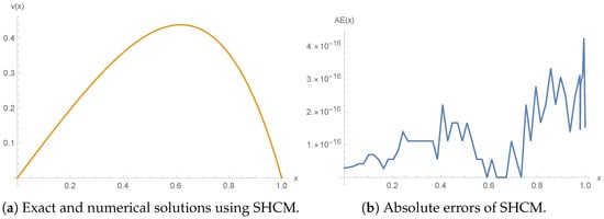
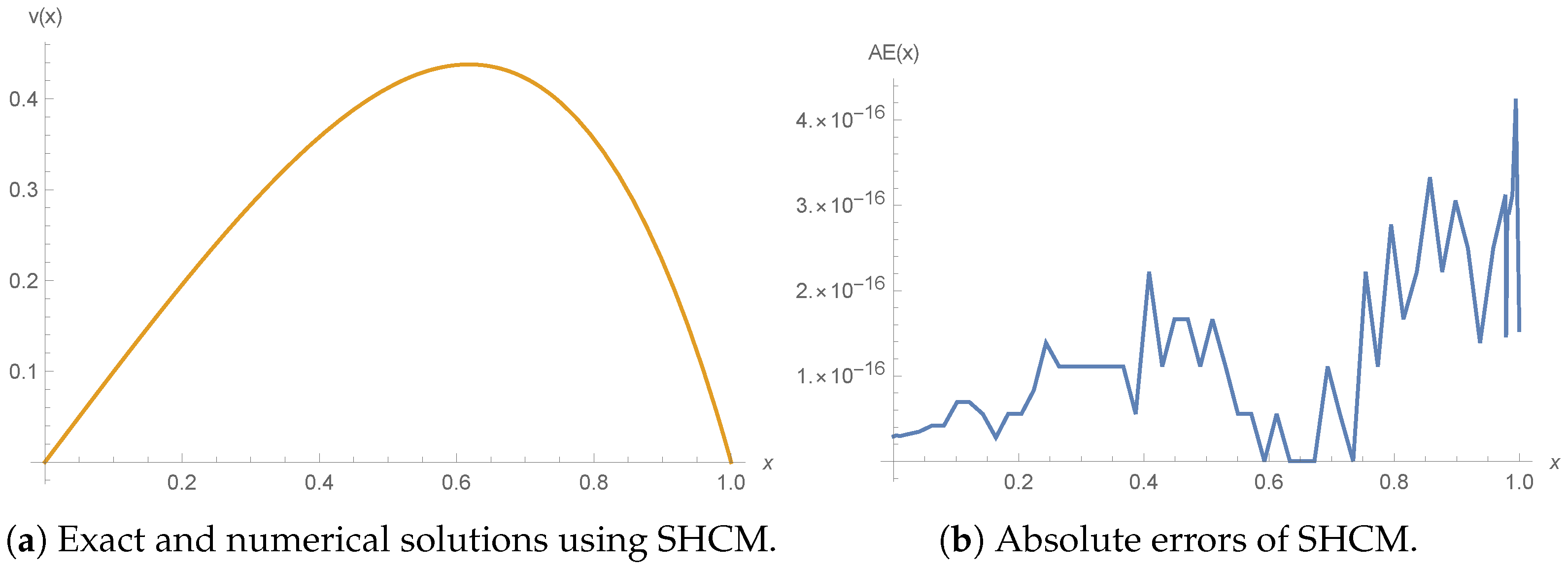
Example 1. Table 1 shows the comparison of the absolute errors and maximum absolute errors of the present method and other existing methods. It is clearly observed that the present method yields higher accuracy compared to the methods presented in [3,8,19,20,21], even for a smaller degree of approximating polynomials. The graphs of the exact and shifted Horadam polynomial series solutions are plotted in Figure 1a, while the graph of the absolute errors is shown in Figure 1b.

Table 1. Comparison of absolute errors of the present method and the methods presented in [3,8,19,20,21] for Example 1.

x	Present Method	Method [3]	Method [8]	Method [21]	Method [20]	Method [19]
$0.1$	$4.06\times {10}^{-17}$	-	$5.55\times {10}^{-9}$	$5.21\times {10}^{-8}$	$1.44\times {10}^{-7}$	$1.02\times {10}^{-6}$
$0.2$	$3.66\times {10}^{-17}$	-	$3.57\times {10}^{-8}$	$2.22\times {10}^{-6}$	$1.45\times {10}^{-6}$	$1.46\times {10}^{-6}$
$0.3$	$5.37\times {10}^{-17}$	-	$4.55\times {10}^{-8}$	$7.00\times {10}^{-6}$	$4.38\times {10}^{-6}$	$1.46\times {10}^{-6}$
$0.4$	$1.32\times {10}^{-16}$	-	$2.79\times {10}^{-8}$	$1.11\times {10}^{-5}$	$7.59\times {10}^{-6}$	$9.14\times {10}^{-7}$
$0.5$	$5.90\times {10}^{-17}$	-	$1.60\times {10}^{-7}$	$1.22\times {10}^{-5}$	$9.06\times {10}^{-6}$	$6.12\times {10}^{-9}$
$0.6$	$6.62\times {10}^{-17}$	-	$2.47\times {10}^{-7}$	$8.88\times {10}^{-6}$	$7.81\times {10}^{-6}$	$8.99\times {10}^{-7}$
$0.7$	$3.77\times {10}^{-17}$	-	$2.11\times {10}^{-7}$	$2.53\times {10}^{-6}$	$4.64\times {10}^{-6}$	$1.44\times {10}^{-6}$
$0.8$	$1.30\times {10}^{-16}$	-	$9.44\times {10}^{-8}$	$1.81\times {10}^{-6}$	$1.58\times {10}^{-6}$	$1.43\times {10}^{-6}$
$0.9$	$1.48\times {10}^{-16}$	-	$1.18\times {10}^{-8}$	$2.04\times {10}^{-6}$	$1.61\times {10}^{-7}$	$9.88\times {10}^{-7}$
MAE	$1.48\times {10}^{-16}$	$8.06\times {10}^{-12}$	$2.47\times {10}^{-7}$	$1.22\times {10}^{-5}$	$9.06\times {10}^{-6}$	$1.46\times {10}^{-6}$

The hyphen “-” indicates that the numerical value at x was not provided.

Figure 1. Comparison of exact and numerical solutions for Example 1.

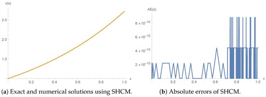
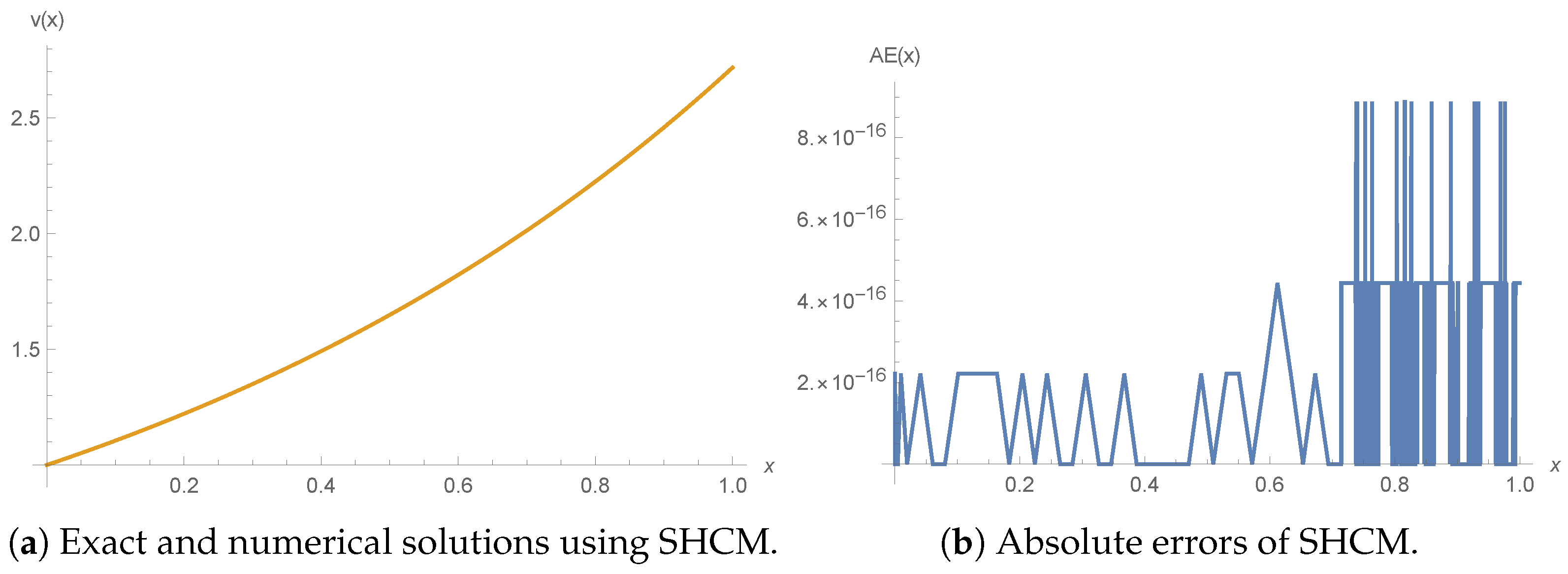
Example 2. Table 2 demonstrates the comparison of the absolute errors and maximum absolute errors of the present method and other existing methods in [3,8,24]. The results show that the present method performs better than the methods under comparison. The graphs of the exact and shifted Horadam polynomial series solutions are plotted in Figure 2a, while the graph of the absolute errors is shown in Figure 2b.

Table 2. Comparison of absolute errors of the present method and those in [2,3,8,24] for Example 2.

x	Present Method	Method [3]	Method [8]	Method I [24]	Method II [24]	Method [2]
$0.1$	$8.21\times {10}^{-17}$	-	$8.57\times {10}^{-11}$	$5.43\times {10}^{-7}$	$8.54\times {10}^{-6}$	$0.61\times {10}^{-8}$
$0.2$	$1.03\times {10}^{-17}$	-	$5.75\times {10}^{-10}$	$7.34\times {10}^{-7}$	$1.73\times {10}^{-6}$	$3.07\times {10}^{-8}$
$0.3$	$1.02\times {10}^{-16}$	-	$8.60\times {10}^{-10}$	$9.54\times {10}^{-7}$	$1.33\times {10}^{-6}$	$4.22\times {10}^{-8}$
$0.4$	$5.34\times {10}^{-19}$	-	$8.45\times {10}^{-12}$	$1.73\times {10}^{-7}$	$2.97\times {10}^{-6}$	$4.97\times {10}^{-8}$
$0.5$	$6.60\times {10}^{-17}$	-	$1.78\times {10}^{-9}$	$4.99\times {10}^{-8}$	$9.49\times {10}^{-7}$	$5.23\times {10}^{-8}$
$0.6$	$3.55\times {10}^{-17}$	-	$3.05\times {10}^{-9}$	$2.40\times {10}^{-7}$	$1.24\times {10}^{-6}$	$4.97\times {10}^{-8}$
$0.7$	$2.42\times {10}^{-16}$	-	$2.70\times {10}^{-9}$	$4.30\times {10}^{-8}$	$9.54\times {10}^{-6}$	$4.23\times {10}^{-8}$
$0.8$	$2.27\times {10}^{-16}$	-	$1.22\times {10}^{-9}$	$7.75\times {10}^{-7}$	$7.75\times {10}^{-7}$	$3.08\times {10}^{-8}$
$0.9$	$1.94\times {10}^{-16}$	-	$1.55\times {10}^{-10}$	$3.20\times {10}^{-7}$	$2.32\times {10}^{-6}$	$1.61\times {10}^{-7}$
MAE	$2.42\times {10}^{-16}$	$2.01\times {10}^{-12}$	$3.05\times {10}^{-9}$	$9.54\times {10}^{-7}$	$9.54\times {10}^{-6}$	$5.23\times {10}^{-8}$

The hyphen “-” indicates that the numerical value at x was not provided.

Figure 2. Comparison of exact and numerical solutions for Example 2.

The numerical solutions obtained give a set of discrete values representing displacement, velocity, acceleration, and higher-order internal forces at specific spatial or temporal mesh points. The numerical solutions in series form also reveal the intricate influence of the system parameters ${\xi }_i,{\eta }_i$$(i=1,2,3,4)$ on the dynamic behavior. Via the numerical solutions obtained, one can study the stability and sharp gradients. The two-dimensional graphs of solutions of the considered eighth-order problems visualise how physical quantities change across space through time simultaneously. The figures translate the visual properties of the x and v axes into real-world physical quantities and behaviour. The x-axis represents the independent variable controlled in an experiment involving time, position, or applied force. The v-axis depicts the dependent variable responding to the change such as displacement, velocity, or potential difference.

6. Conclusions

In this paper, an efficient collocation method based on shifted Horadam polynomials has been applied to obtain numerical solutions of a fourth-order boundary value problem arising in advanced structural mechanics and fluid dynamics such as the radial or vertical deflection of specialised beam-columns, magneto-hydrodynamic stability, and thermal convection layers. For comparison purposes, we considered known examples from published papers. It is clear that in each of the examples considered, the numerical solutions obtained using the present method yielded higher accuracy compared to other existing results. The present method can be extended to the fractional-order version of the governing eighth-order boundary value problem. The correct use of fractional-order differential equations provides more accurate and realistic modeling of memory and hereditary properties in real-world problems.

References

- Davidson, F.A.; Ryne, B.P. The formulation of second-order boundary value problems on time scales. Adv. Differ. Equ. 2006, 2006, 1–10. [Google Scholar] [CrossRef] [Scilit]
- Akram, G.; Rehman, H.U. Numerical solution of eighth order boundary value problems in reproducing kernel space. Numer. Algorithms 2013, 62, 527–540. [Google Scholar] [CrossRef] [Scilit]
- Amin, R.; Shah, K.; Al-Mdallal, Q.M.; Khan, I. Efficient numerical algorithm for the solution of eight order boundary value problems by Haar wavelet method. Int. J. Appl. Comput. Math. 2021, 7, 34. [Google Scholar] [CrossRef] [Scilit] [PubMed]
- Awonusika, R.O. Analytical solutions of generalised Emden–Fowler initial and boundary value problems of higher order. Int. J. Appl. Comput. Math. 2024, 10, 43. [Google Scholar] [CrossRef] [Scilit]
- Costabile, F.A.; Napoli, A. Collocation for high order differential equations with two-points Hermite boundary conditions. Appl. Numer. Math. 2015, 87, 157–167. [Google Scholar] [CrossRef] [Scilit]
- Roul, P. A higher-order B-spline collocation method for solving a class of nonlinear singular boundary value problems. J. Math. Chem. 2024, 62, 1308–1322. [Google Scholar] [CrossRef] [Scilit]
- Boutayeb, A.; Twizell, E.H. Finite-difference methods for the solution of special eighth-order boundary value problems. Int. J. Comput. Math. 1993, 48, 63–75. [Google Scholar] [CrossRef] [Scilit]
- Kumar, R.; Aeri, S.; Sharma, P. Numerical solution of eight order boundary value problems by using Vieta-Lucas polynomials. In Advances in Mathematical Modelling, Applied Analysis and Computation. ICMMAAC 2022; Singh, J., Anastassiou, G.A., Baleanu, D., Kumar, D., Eds.; Lecture Notes in Networks Systems; Springer: Cham, Switzerland, 2022; Volume 666. [Google Scholar] [CrossRef] [Scilit]
- Siddiqi, S.S.; Twizell, E.H. Spline solutions of linear eighth-order boundary-value problems. Comput. Meth. Appl. Mech. Eng. 1996, 131, 457–464. [Google Scholar] [CrossRef] [Scilit]
- Akram, G.; Siddiqi, S. Nonic spline solutions of eighth order boundary value problems. Appl. Math. Comput. 2006, 182, 829–845. [Google Scholar] [CrossRef] [Scilit]
- Siddiqi, S.S.; Akram, G. Solution of eighth-order boundary value problems using the non-polynomial spline technique. Int. J. Comput. Math. 2007, 182, 347–368. [Google Scholar] [CrossRef] [Scilit]
- Liu, G.R.; Wu, T.Y. Differential quadrature solutions of eighth-order boundary-value differential equations. J. Comput. Appl. Math. 2002, 145, 223–235. [Google Scholar] [CrossRef] [Scilit]
- Inc, M.; Evans, D.J. An efficient approach to approximate solutions of eighth-order boundary value problems. Int. J. Comput. Math. 2004, 81, 685–692. [Google Scholar] [CrossRef] [Scilit]
- He, J.H. The variational iteration method for eighth-order initial-boundary value problems. Phys. Scr. 2007, 76, 680–682. [Google Scholar] [CrossRef] [Scilit]
- Porshokouhi, M.G.; Ghanbari, B.; Gholami, M.; Rashidi, M. Numerical solution of eighth order boundary value problems with variational iteration method. Gen. Math. Notes 2011, 2, 128–133. [Google Scholar]
- Mestrovic, M. The modified decomposition method for eighth-order boundary value problems. Appl. Math. Comput. 2007, 188, 1437–1444. [Google Scholar] [CrossRef] [Scilit]
- Noor, M.A.; Mohyud-Din, S.T. Variational iteration decomposition method for solving eighth-order boundary value problems. Differ. Equ. Nonlinear Mech. 2007, 2007, 1–16. [Google Scholar] [CrossRef] [Scilit]
- Golbabai, A.; Javidi, M. Application of homotopy perturbationmethod for solving eighth order boundary value problems. Appl. Math. Comput. 2007, 191, 334–346. [Google Scholar] [CrossRef] [Scilit]
- Raji, M.T.; Christie, I.Y.; Babalola, O.O.; Ayoola, T.A.; Momoh, N.M.; Peter, O.J. Numerical solution of eighth order boundary value problems using Chebyshev polynomials. Math. Comput. Sci. 2023, 4, 18–28. [Google Scholar]
- Elahi, Z.; Akram, G.; Siddiqi, S.S. Numerical solution for solving special eighth-order linear boundary value problems using Legendre Galerkin method. Math. Sci. 2016, 10, 201–209. [Google Scholar] [CrossRef] [Scilit]
- Viswanadham, K.N.S.K.; Ballem, S. Numerical solution of eighth order boundary value problems by Galerkin method with quintic b-splines. Int. J. Comput. Appl. 2014, 89, 7–13. [Google Scholar] [CrossRef] [Scilit]
- Abd-Elhameed, W.M.; Alqubori, O.M.; Atta, A.G. A collocation approach for the nonlinear fifth-order KdV equations using certain shifted Horadam polynomials. Mathematics 2025, 13, 300. [Google Scholar] [CrossRef] [Scilit]
- Wanas, A.K. Horadam polynomials for a new family of λ-pseudo bi-univalent functions associated with Sakaguchi type functions. Afr. Mat. 2021, 32, 879–889. [Google Scholar] [CrossRef] [Scilit]
- Islam, M.S.; Hossain, M.B. Numerical solutions of eighth order BVP by the Galerkin residual technique with Bernstein and Legendre polynomials. Appl. Math. Comput. 2015, 261, 48–59. [Google Scholar] [CrossRef] [Scilit]
Disclaimer/Publisher’s Note: The statements, opinions and data contained in all publications are solely those of the individual author(s) and contributor(s) and not of MDPI and/or the editor(s). MDPI and/or the editor(s) disclaim responsibility for any injury to people or property resulting from any ideas, methods, instructions or products referred to in the content. |
© 2026 by the author. Licensee MDPI, Basel, Switzerland. This article is an open access article distributed under the terms and conditions of the Creative Commons Attribution (CC BY) license.