


Simple Summary
This study shows that machine learning can effectively identify reported Rift Valley fever occurrence from climatic and environmental conditions despite severe class imbalance, with tree-based ensemble models providing the strongest discrimination and highlighting rainfall, seasonality, and terrain as important factors, although prospective early-warning applications will require temporally and geographically independent validation.
Abstract
Rift Valley fever (RVF) is a vector-borne zoonotic disease whose occurrence is strongly associated with climatic and environmental conditions, making data-driven approaches potentially valuable for epidemiological surveillance and risk assessment. Using a publicly available historical dataset comprising 180,288 monthly observations from geographically defined administrative units across Kenya between 1981 and 2010, this study investigates machine learning (ML) for the retrospective classification of reported RVF occurrence from contemporaneous climatic, environmental, topographic, and seasonal predictors under an extremely imbalanced classification setting. The dataset provides broad geographic coverage across Kenya over a 30-year historical period; however, because the outcome reflects reported events in historical surveillance records, it is not assumed to constitute a formally population-representative national sample or to capture all underlying RVF transmission. Each observation represents a geographic unit and observation month, and the response indicates whether an RVF event was reported during that corresponding period. Therefore, the present analysis should be interpreted as contemporaneous outbreak classification rather than as a fixed-horizon prospective forecast. Thirteen classifiers representing distinct learning paradigms were systematically evaluated: Logistic Regression, Linear Discriminant Analysis, K-Nearest Neighbors, Classification and Regression Tree, Naive Bayes, Support Vector Machine, Weighted Logistic Regression, XGBoost, LightGBM, CatBoost, Balanced Random Forest, EasyEnsemble, and RUSBoost. Model performance was assessed before and after SMOTENC-based rebalancing using overall and class-specific metrics, including accuracy, precision, sensitivity, specificity, F1-score, ROC–AUC, and precision–recall-based measures. Under the retrospective stratified hold-out benchmark, XGBoost, CatBoost, Balanced Random Forest, and LightGBM achieved ROC–AUC values of 0.9176, 0.9175, 0.9114, and 0.9062, respectively. Balanced Random Forest attained the highest outbreak sensitivity (0.8851), although at the cost of very low precision, illustrating that high rare-event detection can generate a substantial false-alert burden in surveillance settings. SMOTENC produced strongly model-dependent effects: it increased outbreak sensitivity for XGBoost, LightGBM, CatBoost, KNN, CART, and RUSBoost, but substantially reduced sensitivity for Balanced Random Forest and EasyEnsemble. SHAP-based interpretability analysis indicated that month, rainfall, and slope were among the most influential predictors and further showed that class rebalancing can alter the distribution of feature contributions. Overall, the findings demonstrate that modeling reported RVF occurrence under severe class imbalance requires joint evaluation of minority-class detection, false-positive behavior, discrimination, and model interpretability rather than overall accuracy alone. The present results establish a retrospective classification benchmark for climate-informed RVF risk assessment, but they should not be interpreted as an autonomous outbreak-warning system. Translation into prospective early-warning prediction will require an explicit forecasting horizon, predictors constructed exclusively from information available before the target period, temporally and geographically independent validation, and decision thresholds evaluated against an operationally acceptable false-alert burden.
1. Introduction
Rift Valley fever (RVF) is a mosquito-borne zoonotic disease of considerable veterinary, socioeconomic, and public health importance, particularly in Sub-Saharan Africa and the Arabian Peninsula. The disease is caused by Rift Valley fever virus (RVFV), a pathogen that primarily affects domesticated ruminants and can also infect humans [1]. RVFV is currently classified within the family Phenuiviridae and the order Hareavirales [2]. The virus was first identified in 1931 following an outbreak among sheep on a farm in Kenya’s Rift Valley Province [3]. Since then, recurrent outbreaks have demonstrated the capacity of RVF to simultaneously affect animal production systems, rural livelihoods, food security, and human health. These consequences are particularly important for pastoral and agro-pastoral communities, whose economic activities and subsistence are strongly dependent on livestock [4].
In humans, the incubation period following exposure to RVFV generally ranges from 2 to 6 days [5]. Although most human infections are self-limiting, severe clinical manifestations can occur, and fatal outcomes have been reported in approximately 1% of infected individuals [6]. From the veterinary perspective, the impact of RVF can be substantially greater. The virus is particularly pathogenic in sheep, followed by goats and cattle [7]. Outbreaks in susceptible livestock populations are commonly characterized by fever, weakness, high mortality among young animals, and extensive reproductive losses. Pregnant animals are particularly vulnerable, with abortion rates approaching 100% during severe outbreaks [8]. In contrast, adult animals generally exhibit lower mortality and less severe clinical manifestations [9]. These characteristics make RVF not only an infectious-disease problem but also an important threat to livestock productivity, animal trade, household income, and regional food systems. More broadly, the emergence and re-emergence of zoonotic diseases are influenced by interactions among human activities, environmental change, agricultural intensification, land-use modification, and increasing interfaces between humans, domestic animals, wildlife, and disease vectors, reinforcing the importance of integrated One Health approaches to zoonotic-disease surveillance and prevention [10].
A major challenge in RVF surveillance is its close association with climatic and environmental conditions. RVF is considered a climate-sensitive zoonosis, and the timing and spatial distribution of reported outbreaks have been associated with interactions among rainfall, temperature, humidity, vegetation, hydrological conditions, vector ecology, and host availability [11]. Anomalous rainfall and elevated humidity may create conditions favorable to the emergence, survival, and proliferation of mosquito vectors, including species of the genus Aedes [12,13], whereas lower temperatures can constrain mosquito activity, development, and reproduction [14]. These relationships are not necessarily instantaneous or linear because environmental conditions may influence vector populations and transmission processes over different temporal scales.
Periods of excessive rainfall and flooding are especially relevant to RVF epidemiology because they can generate temporary aquatic habitats favorable to mosquito emergence. In East Africa, these environmental anomalies have frequently been associated with El Niño–Southern Oscillation (ENSO) events and have contributed to approaches for anticipating RVF activity [15]. Associations have also been reported between RVF occurrence and humidity, vegetation, land-cover, and soil-related characteristics, supporting the view that outbreak risk reflects combinations of environmental conditions rather than a single climatic determinant [3,16]. Importantly, the temporal relationship between environmental exposure and epidemiological outcome determines how such information can be interpreted. Measurements obtained during the same period as an outbreak support contemporaneous risk characterization, whereas prospective early-warning prediction requires predictors constructed exclusively from information available before the target period, such as lagged climatic variables or preceding-period environmental summaries.
One Health Perspective
RVF provides a clear One Health setting because transmission links environmental conditions, mosquito vectors, susceptible livestock, and human exposure within the same epidemiological process. Livestock occupy a particularly important position in this interface: infection affects animal health and production while also creating opportunities for human exposure through contact with infected animals, biological materials, and environments in which competent vectors are active. Environmental conditions influence this interface by modifying vector habitats and the spatial and seasonal conditions under which transmission can occur. Thus, RVF surveillance requires information from domains that are biologically connected but traditionally monitored by different sectors [10].
The present study addresses one specific component of this One Health system: the environmental and seasonal context associated with reported RVF occurrence. Climatic, topographic, edaphic, and seasonal predictors can indicate conditions under which reported events are more likely to occur, but they do not directly measure infection in livestock, vector abundance, human exposure, or viral circulation. The resulting machine learning models should therefore be viewed as an environmental risk-assessment layer that may complement veterinary, entomological, epidemiological, and laboratory surveillance rather than as a complete representation of RVF transmission. In practical terms, a positive model output should be interpreted as a risk signal that can prioritize a location or period for additional investigation, not as independent confirmation of an outbreak. This distinction defines both the scope of the present analysis and the potential role of its predictions within an integrated One Health surveillance framework.
The increasing availability of epidemiological, environmental, and climatic data provides opportunities to complement conventional surveillance with data-driven computational approaches. Artificial intelligence and machine learning (ML) methods have been widely applied to classification, prediction, and pattern-recognition problems in domains including financial forecasting, fraud detection, medical diagnosis, speech recognition, and image analysis [17,18]. In infectious-disease epidemiology, ML is particularly attractive because outbreak occurrence may depend on nonlinear relationships, higher-order interactions, seasonality, spatial heterogeneity, and combinations of epidemiological and environmental signals that are difficult to represent with simple parametric assumptions. At the same time, infectious-disease forecasting is methodologically demanding: the unit of prediction and forecasting horizon must be defined in advance, predictors must be restricted to information available before the target event, and evaluation must respect temporal and, when relevant, geographic separation. Otherwise, retrospective discrimination can be mistaken for prospective forecasting ability.
Recent computational studies of RVF illustrate the broader movement toward machine-learning-assisted infectious-disease surveillance and forecasting. Mulwa et al. [19] used XGBoost with climatic information to model RVF outbreak occurrence in Kenya, showing the potential of nonlinear ensemble learning for climate-informed disease prediction. More recently, Mulwa et al. [20] compared multiple machine learning classifiers on historical Kenyan RVF data and demonstrated that excellent overall accuracy can coexist with very poor detection of the rare outbreak class. Complementing these ML approaches, Angelakis et al. [21] modeled sparse monthly RVF incidence in northern Kenya using zero-inflated Bayesian methods and highlighted the predictive relevance of lagged climatic information. Taken together, these recent studies show that contemporary infectious-disease prediction increasingly requires not only flexible algorithms but also explicit attention to temporal structure, sparse outcomes, predictor timing, and the distinction between retrospective classification and genuine early-warning forecasting.
The same literature also emphasizes that performance cannot be judged by a single global metric when the event of interest is rare. In low-prevalence surveillance settings, high accuracy, specificity, or even strong ROC–AUC can coexist with low positive predictive value and a large number of false alerts. This has direct operational consequences because each false-positive prediction may trigger epidemiological review, veterinary field investigation, entomological assessment, laboratory testing, or other resource-intensive activities. Therefore, an operationally useful infectious-disease model should be evaluated simultaneously in terms of discrimination, minority-class sensitivity, precision, false-positive burden, calibration or threshold behavior, and transportability across time and space. These requirements are particularly important for RVF because reported outbreaks represent only a very small fraction of the available historical observations.
Broader disease-prediction research also demonstrates the flexibility of modern ensemble methods while underscoring the need for domain-specific validation. XGBoost, for example, has attracted considerable attention because of its ability to model nonlinear relationships and interactions, incorporate regularization, and operate effectively on structured datasets containing multiple predictors [22]. Recent applications in health prediction have reported competitive performance for gradient-boosting methods [23], and comparisons involving diseases such as diabetes and cardiovascular disorders have reported better predictive performance for XGBoost than for logistic regression (LR) and random forest (RF) under the evaluated experimental settings [24]. However, performance observed in non-infectious disease datasets cannot be directly generalized to RVF because prevalence, sample size, predictor characteristics, temporal dependence, geographic structure, and the operational costs of false predictions differ substantially across applications.
Although numerous studies have investigated the economic and epidemiological consequences of livestock diseases, comparatively fewer investigations have systematically evaluated how different machine learning paradigms behave when climatic and environmental predictors are combined with the extreme class imbalance characteristic of RVF surveillance data. The unresolved problem is therefore not simply whether an algorithm can achieve high global predictive performance. A useful framework must determine whether rare reported events can be detected without creating an impractical false-positive burden, whether performance persists under more restrictive temporal and geographic validation, and whether the environmental variables driving model decisions remain interpretable after imbalance-handling procedures are applied.
Within this context, the present study investigates the retrospective classification of reported RVF occurrence from contemporaneous climatic, environmental, topographic, and seasonal information under severe class imbalance. Thirteen classifiers representing distinct methodological families are systematically evaluated: Logistic Regression (LR), Linear Discriminant Analysis (LDA), K-Nearest Neighbors (KNN), Classification and Regression Tree (CART), Naive Bayes (NB), Support Vector Machine (SVM), Weighted Logistic Regression (WLR), XGBoost, LightGBM, CatBoost, Balanced Random Forest (BRF), EasyEnsemble, and RUSBoost. Rather than establishing a simple ranking of algorithms, the analysis examines how different learning strategies balance rare-event detection, specificity, precision, and false-positive generation.
A central component of the study is the controlled evaluation of SMOTENC across these model families by comparing classifier behavior before and after rebalancing under the same experimental framework. Performance is assessed using overall and minority-class-oriented measures, including sensitivity, specificity, false-negative rate, precision, F1-score, ROC–AUC, and precision–recall-based metrics. This design makes it possible to distinguish improvements in global discrimination from improvements in the detection of the rare RVF class and to identify situations in which increased sensitivity may be obtained at an operationally unfavorable cost in false-positive alerts.
The study also incorporates SHAP-based interpretability analysis to examine the predictive contribution of environmental and seasonal variables and whether their attribution patterns change after class rebalancing. The contribution of the work therefore lies in jointly evaluating four interdependent aspects of rare-event RVF classification: model discrimination, minority-class detection under different imbalance-handling strategies, false-positive burden with implications for surveillance feasibility, and the stability of model interpretation after resampling. The study does not treat retrospective classification performance as evidence of a deployable early-warning system; rather, it establishes a benchmark from which operational thresholds, prospective forecasting horizons, and independent temporal and geographic validation can be developed. These components provide complementary evidence for assessing how environment-informed machine learning may be incorporated responsibly into RVF risk assessment while recognizing the limitations of the available surveillance outcome.
The remainder of this article is organized as follows. Section 2 presents the related work, reviewing previous statistical, environmental, and machine learning approaches for Rift Valley fever modeling and highlighting challenges associated with extreme class imbalance, rare-event detection, and model interpretability. Section 3 describes the materials and methods, including the study area, dataset and predictor variables, preprocessing, SMOTENC-based rebalancing, the thirteen classifiers, hyperparameter optimization, validation strategies, performance metrics, and SHAP-based interpretability analysis. Section 4 reports the experimental results for the original and rebalanced training conditions. Section 5 discusses the findings, including their One Health interpretation, minority-class performance, false-positive burden, resampling effects, and temporal scope. Finally, Section 6 summarizes the main conclusions, limitations, and directions for future investigation.
2. Related Work
Rift Valley fever (RVF) is a climate-sensitive zoonotic disease whose epidemiology is strongly influenced by environmental, ecological, and seasonal conditions. Climatic anomalies, particularly those associated with the El Niño–Southern Oscillation (ENSO), have been repeatedly associated with RVF activity because variations in rainfall, temperature, humidity, vegetation, and hydrological conditions affect mosquito emergence, vector abundance, and the environmental suitability for transmission [12,25,26]. Consequently, the integration of epidemiological observations with climatic and environmental information has become an important component of RVF risk assessment and predictive modeling.
Early data-driven approaches focused primarily on spatial and environmental characterization of RVF risk. Palaniyandi [27] explored remotely sensed information to identify environmental conditions associated with vector-breeding habitats. Similarly, Soti et al. [28] combined very-high-resolution satellite imagery, landscape characteristics, and beta-binomial regression to identify areas associated with RVFV transmission in Senegal. These studies demonstrated the value of vegetation, temporary water bodies, and landscape structure for characterizing transmission risk, although their primary objective was spatial risk mapping rather than comparative outbreak classification.
Environmental determinants have also been investigated through vector-oriented and One Health approaches. Talla et al. [29] used generalized linear mixed models to examine climatic and environmental factors associated with hotspots of Aedes vexans and Culex poicilipes in Senegal, showing that temperature, humidity, and spatial characteristics contribute to variations in mosquito abundance. Bashir and Hassan [30] integrated epidemiological, environmental, remote-sensing, and geographic information to investigate RVF transmission in Sudan from a One Health perspective. Although these approaches strengthened the epidemiological understanding of environmental drivers, they were not designed to systematically compare machine learning classifiers under severe class imbalance.
More flexible statistical and computational strategies subsequently expanded the modeling of RVF occurrence. Nicholas et al. [31] applied geographically weighted discriminant analysis to environmental data from South Africa and demonstrated that explicitly accounting for spatial heterogeneity improved classification relative to conventional discriminant analysis. Hardcastle et al. [32] employed boosted regression trees to estimate monthly environmental suitability for RVF across Africa, Europe, and the Middle East, showing the capacity of nonlinear tree-based methods to identify complex spatial and seasonal patterns. These studies provided important evidence for nonlinear environmental modeling, although their objectives were primarily spatial suitability assessment rather than systematic comparison of rare-event classifiers.
Temporal sparsity represents an additional challenge in RVF modeling. Angelakis et al. [21] investigated zero-inflated Bayesian models for sparse monthly RVF incidence in northern Kenya and showed that explicitly accounting for the large number of zero observations improved predictive modeling. Their analysis also identified the relevance of lagged climatic information, with rainfall at a three-month lag contributing to the best-performing model. In a different methodological direction, Xue et al. [33] developed a network-based metapopulation model integrating humans, livestock, mosquito vectors, spatial movement, and weather-dependent parameters. Together, these studies highlight that RVF dynamics involve temporal dependence, environmental forcing, and heterogeneous transmission mechanisms that cannot be fully represented by simple static relationships.
More recently, machine learning has been directly investigated for RVF prediction in Kenya. Mulwa et al. [19] applied XGBoost to historical RVF observations and climatic predictors, demonstrating the potential of gradient-boosted trees for identifying nonlinear relationships associated with outbreak occurrence. This study represented an important step toward the use of modern ensemble learning for climate-informed RVF prediction, but its methodological emphasis was primarily on XGBoost rather than on the comparative behavior of different learning paradigms and imbalance-handling strategies.
A subsequent study by Mulwa et al. [20], published in Zoonotic Diseases, substantially broadened this perspective by evaluating multiple classifiers on historical RVF data from Kenya covering 1981–2010. The study compared Logistic Regression, Linear Discriminant Analysis, K-Nearest Neighbors, Classification and Regression Tree, Naive Bayes, Support Vector Machine, Random Forest, and XGBoost and evaluated their performance using conventional classification measures together with ROC- and precision–recall-based metrics. Importantly, the results exposed a central difficulty of this dataset: classifiers could achieve very high overall accuracy and specificity while exhibiting very low or even zero sensitivity for RVF outbreaks. This finding established that the major methodological challenge is not simply obtaining high overall classification performance, but learning useful decision functions when outbreak observations represent an extremely small fraction of the available data.
Table 1 summarizes representative computational, statistical, and machine learning studies on RVF and highlights their main methodological contributions and remaining limitations. The comparison shows the progression from spatial and environmental risk characterization toward more flexible nonlinear and machine learning approaches. It also indicates that, although recent studies have already compared multiple classifiers for RVF prediction, the combined effects of extreme class imbalance, explicit rebalancing strategies, minority-class-oriented evaluation, and model interpretability remain comparatively underexplored.
Table 1.
Comparison of representative studies on computational, environmental, and machine learning approaches for Rift Valley fever modeling.
Accordingly, the current research gap can no longer be characterized simply as a lack of comparative machine learning studies for RVF. Instead, an important unresolved question concerns how different learning paradigms behave when extreme outbreak rarity is explicitly addressed during model development. Specifically, limited evidence is available on whether synthetic class rebalancing produces consistent improvements across conventional classifiers, gradient-boosting methods, cost-sensitive approaches, and ensemble algorithms that already incorporate mechanisms for handling imbalance. This distinction is important because an apparent improvement in overall performance may coexist with deterioration in outbreak sensitivity, precision, or false-positive control.
A second unresolved issue concerns model interpretability under resampling. Previous studies have investigated environmental associations, correlations, feature relevance, and predictive performance; however, substantially less attention has been given to whether modifying the training distribution changes the explanatory structure learned by the classifier. This is particularly relevant for epidemiological applications, in which climatic and environmental variables are interpreted not only as predictive inputs but also as indicators of conditions associated with increased outbreak risk. Consequently, resampling should be evaluated not only according to its effect on classification metrics but also according to its effect on model attribution and the stability of predictor importance.
The present study addresses these gaps through a standardized comparison of thirteen classifiers encompassing linear, probabilistic, instance-based, margin-based, tree-based, gradient-boosting, cost-sensitive, and imbalance-oriented ensemble approaches. Each classifier is evaluated under the original training distribution and after SMOTENC-based partial rebalancing, while the independent test distribution remains unchanged. Performance is examined through overall and class-specific measures, with particular attention to outbreak sensitivity, false-negative and false-positive behavior, ROC–AUC, and precision–recall-based performance. In addition, SHAP-based analyses are used to determine whether class rebalancing modifies the relative contribution of climatic, environmental, and seasonal predictors. Therefore, rather than providing another classifier ranking, this study focuses on the interaction between learning strategy, extreme class imbalance, synthetic rebalancing, minority-class detection, and model interpretability.
3. Materials and Methods
3.1. Study Area
Kenya was selected as the study area because Rift Valley fever (RVF) has historically represented an important zoonotic and livestock-health concern in the country, with reported outbreaks exhibiting marked spatial and temporal heterogeneity. The dataset analyzed in this study covers a 30-year period, from 1981 to 2010, and contains monthly observations associated with geographically defined administrative units distributed throughout Kenya.
The analytical structure of the dataset is therefore inherently spatiotemporal: observations from the same geographic unit may occur repeatedly across different months and years, while observations from different geographic units may occur during the same time period. This structure is epidemiologically relevant because RVF occurrence may exhibit both temporal dependence, resulting from seasonality and persistent climatic conditions, and spatial dependence, resulting from shared environmental, hydrological, ecological, and geographic characteristics among neighboring or repeatedly observed locations.
Figure 1 shows the spatial distribution of reported RVF events across the administrative units represented in the dataset during the 1981–2010 study period. Considerable geographic heterogeneity is evident, with reported events concentrated in selected areas rather than uniformly distributed across the country. This spatially clustered structure motivated the inclusion of geographically grouped validation in addition to conventional random partitioning, as described in Section 3.3.
Figure 1.
Spatial distribution of reported Rift Valley fever (RVF) events across Kenya from 1981 to 2010. Administrative units are colored according to the number of recorded RVF events, ranging from no reported events to 30–65 reported events, while dashed green lines indicate provincial boundaries. The map illustrates the marked spatial heterogeneity of reported RVF occurrence across the study area.
The presence of repeated observations across administrative units and over multiple years has direct implications for predictive-model validation. Randomly allocating individual observations to training and test sets may place temporally adjacent observations or repeated measurements from the same geographic unit in both subsets. Consequently, model performance estimated exclusively from a random partition may characterize interpolation within the historical data distribution more accurately than generalization to future periods or previously unseen geographic areas. For this reason, the present study distinguishes retrospective random-split performance from temporal and spatial generalization performance.
3.2. Dataset Structure, Outcome Definition, and Predictor Selection
The dataset consists of monthly observations recorded for geographically defined administrative units in Kenya between 1981 and 2010. Each analytical observation represents the environmental and climatic conditions associated with a specific geographic unit and observation month, together with the corresponding RVF reporting status.
The response variable was formulated as a binary outcome indicating whether an RVF event was recorded for the corresponding geographic unit and observation period. Observations coded as 1 represent a reported RVF event, whereas observations coded as 0 represent periods for which no RVF event was recorded in the source dataset. Accordingly, the negative class is interpreted throughout this study as “no reported outbreak” rather than as definitive evidence of the biological absence of RVF transmission. This distinction is particularly important for historical surveillance data because the sensitivity and coverage of disease-reporting systems may vary across geographic areas and over time.
The candidate environmental predictors describe climatic, topographic, edaphic, and seasonal conditions potentially associated with RVF occurrence. The final predictive feature set comprised month, rainfall, elevation, slope, clay, and relative humidity. Month was treated as a categorical seasonal predictor, whereas rainfall, elevation, slope, clay, and humidity were handled as continuous variables.
Geographic identifiers and calendar year were retained exclusively as structural variables for exploratory analysis and validation design and were not used as direct predictive features in the machine learning models. Specifically, the geographic identifier was used to construct spatially independent validation partitions, whereas year was used to establish chronologically ordered temporal partitions. This separation prevents the models from directly exploiting geographic labels or calendar-year identifiers as surrogate predictors of the outcome and reduces the potential for information leakage.
The climatic and environmental predictors were selected because RVF transmission is strongly influenced by conditions affecting mosquito emergence, vector survival, water accumulation, and the persistence of suitable breeding habitats. Rainfall-related conditions are particularly relevant because increased precipitation and flooding may create temporary water bodies suitable for mosquito emergence. Relative humidity can affect mosquito survival and activity, while elevation and terrain characteristics may influence local hydrological conditions and vector distribution. Soil characteristics, including clay content, may further modify water retention and the persistence of temporary aquatic habitats.
Table 2 summarizes the variables used in the analytical framework and distinguishes predictive features from variables retained exclusively for temporal and spatial validation. To improve reproducibility, the table also reports the available information on variable definition, measurement scale, temporal structure, and analytical role.
Table 2.
Definition and analytical role of the variables used in the RVF machine learning framework.
A similar provenance issue was identified for the terrain variable originally labeled Slope. Its values are tightly concentrated near 90 in the source dataset, including values such as 89.9, and the available source documentation does not specify its unit or mathematical derivation. These values were already present in the original dataset and were not produced by the preprocessing performed in this study. Consequently, the variable was retained numerically as provided but is conservatively referred to as a slope-derived terrain measure. No conversion to degrees or percentage slope was performed, and no direct physical interpretation of its magnitude is assumed.
The final predictive feature matrix therefore comprised month, rainfall, elevation, slope, clay, and humidity. Geographic identifiers and calendar year were retained only to define spatially and temporally independent validation partitions and were not supplied to the classifiers as predictors. The binary RVF outcome was likewise excluded from all predictor-based exploratory analyses.
For exploratory assessment of linear dependence among continuous predictors, Pearson’s correlation coefficient was calculated. Values range from to , with values close to zero indicating weak linear association and values approaching either extreme indicating stronger negative or positive relationships [34]. Only variables with a meaningful continuous scale were included in this analysis. Geographic identifiers, calendar year, and the binary RVF outcome were excluded from the predictor correlation matrix to avoid interpreting arbitrary identifier codes or the target variable as continuous environmental measurements.
The final predictor matrix used for model development was explicitly defined as
The binary RVF status was used exclusively as the response variable . Geographic ID and calendar year were not included in . Instead, Geographic ID was retained only for spatially grouped validation, whereas Year was retained only for temporally ordered validation. Therefore, neither administrative identifiers nor calendar year contributed directly to model fitting or prediction.
Table 3 provides the descriptive and univariate characterization of the continuous environmental variables according to reported RVF status. Because several predictor distributions were non-Gaussian and the two outcome groups were strongly unequal in size, between-group differences were evaluated using the Mann–Whitney U test, while Cliff’s was used as a non-parametric measure of effect size. Statistical significance was interpreted jointly with effect-size magnitude rather than in isolation. Complementarily, Figure 2 presents the Pearson correlation matrix among the continuous predictors, providing an overview of their pairwise linear relationships and allowing the identification of potentially redundant or strongly correlated environmental variables.
Table 3.
Descriptive and univariate statistical analysis of environmental variables according to reported RVF occurrence in Kenya.
Figure 2.
Pearson correlation matrix for the continuous climatic, environmental, and topographic predictors considered in the RVF classification framework. Geographic identifiers, calendar year, and the binary RVF outcome were excluded from this predictor-correlation analysis.
The resulting dataset is characterized by extreme class imbalance. Of the 180,288 observations included in the analytical dataset, 433 correspond to reported RVF events and 179,855 correspond to observations with no reported RVF event. Thus, the positive class represents only approximately 0.24% of the available observations.
This extreme prevalence imbalance motivated the use of minority-class-oriented performance measures and imbalance-aware learning strategies described in the subsequent sections. It also motivated careful validation procedures because apparently high overall accuracy can be obtained even when a classifier has limited ability to identify the rare outbreak class.
Table 4 summarizes the distribution of the reported RVF outcome classes in the analytical dataset. The data reveal a pronounced class imbalance, with reported RVF outbreaks accounting for only 0.24.
Table 4.
Distribution of reported RVF outcome classes in the analytical dataset.
3.3. Data Pre-Processing and Validation Design
The initial dataset comprised 181,801 observations. Before model development, the data were examined for completeness, consistency, duplicate records, invalid categorical values, and potentially anomalous continuous measurements. This data-quality assessment was conducted independently of model performance and before the construction of the validation experiments.
In the original analytical workflow, potentially extreme observations in continuous variables were identified using the interquartile-range (IQR) criterion. For each continuous variable, the first () and third () quartiles were calculated and the interquartile range was defined as
Observations containing values below
or above
were flagged as potentially extreme observations. Binary and categorical variables were not subjected to this criterion and were instead evaluated according to their predefined domains.
Because extreme climatic conditions may be epidemiologically meaningful for RVF rather than representing measurement errors, the IQR criterion was not interpreted as evidence that an observation was biologically implausible. Accordingly, the effect of this preprocessing decision was evaluated separately through a sensitivity analysis comparing model performance with and without IQR-based exclusion. This procedure allows the robustness of the conclusions to be assessed without assuming that statistically extreme environmental conditions are necessarily erroneous.
The final analytical dataset used for the principal comparisons contained 180,288 observations, including 179,855 observations with no reported outbreak and 433 reported RVF-outbreak observations. A complete accounting of records excluded during data-quality processing, including the number of positive and negative observations affected by each exclusion criterion, is reported separately in the revised Section 4.
3.3.1. Validation Strategy
The spatiotemporal structure of the RVF dataset required particular attention during model validation. Because observations were repeatedly collected across geographic units over a 30-year period, a conventional random train–test split alone could allocate observations from the same geographic unit or closely related time periods to both training and test sets. Such a design is useful for estimating retrospective discrimination within the observed historical distribution but may provide optimistic estimates of generalization to future periods or geographically unseen areas.
To explicitly distinguish these forms of generalization, three complementary validation scenarios were considered: (i) a stratified random hold-out benchmark, (ii) temporally separated validation, and (iii) spatially grouped validation.
Retrospective Random Hold-Out Benchmark
For comparability with the original experimental design and with previously reported analyses of this dataset, a stratified random 80:20 train–test partition was retained as a retrospective benchmark. Eighty percent of the observations were allocated to model development and hyperparameter optimization, while the remaining 20% constituted an untouched test set. Stratification was performed according to the binary RVF outcome to preserve, as closely as possible, the extremely low prevalence of reported outbreaks in both subsets.
The pseudo-random seed was fixed at random_state = 42 to ensure reproducibility of the partition. This random-split experiment is explicitly interpreted as an estimate of within-distribution retrospective performance; it is not considered a prospective forecasting experiment because observations from different years and repeated geographic units may occur in both subsets.
Temporal Validation
To assess generalization across time, an additional temporally separated validation experiment was performed. Observations were ordered according to calendar year and complete temporal units were assigned to either model development or evaluation, such that observations from the evaluation period always occurred chronologically after observations used for model training.
The temporal validation procedure did not randomly mix observations across years. Calendar year was used exclusively to define temporal partitions and was not supplied to the classifiers as a predictive feature. Consequently, models evaluated under this design were required to transfer relationships learned from earlier historical periods to observations occurring in later periods.
Hyperparameter optimization for the temporally evaluated models was restricted to observations belonging to the training period. Temporal folds used during model selection preserved chronological ordering, so that validation observations always occurred after the observations used to fit the corresponding candidate model. After hyperparameter selection, the final model was refitted using all observations available in the temporal training period and evaluated on the chronologically subsequent hold-out period.
This design provides a more stringent estimate of temporal transportability than the random hold-out benchmark because future observations cannot contribute to model fitting, preprocessing, resampling, or hyperparameter selection.
Spatially Grouped Validation
A complementary spatial-validation experiment was conducted to evaluate model generalization to geographically unseen administrative units. All observations belonging to the same geographic unit were assigned to the same validation group. Thus, a geographic unit included in an evaluation fold was completely absent from the corresponding training fold.
The geographic identifier was used only as a grouping variable and was not included among the model predictors. Spatial partitions were constructed using group-aware stratified cross-validation whenever feasible, thereby seeking to preserve the rare-event class distribution while maintaining strict geographic separation between training and validation observations.
For a spatial fold k, if denotes the set of geographic units assigned to the evaluation partition and denotes the set assigned to model development, the partitioning procedure enforced
This constraint prevents observations from the same administrative unit from appearing simultaneously in the training and evaluation subsets and therefore provides a more rigorous assessment of geographic transportability.
Interpretation of Validation Scenarios
The three validation strategies answer different predictive questions. The random hold-out benchmark measures discrimination among observations drawn from the same historical data distribution. Temporal validation evaluates whether relationships learned from earlier periods remain informative for later observations. Spatially grouped validation evaluates whether learned relationships transfer to geographic units that were not represented during model fitting.
Accordingly, performance obtained under the random split was not used alone to claim prospective or geographically transferable prediction. Instead, model performance was interpreted jointly across the random, temporal, and spatial validation settings. Particular emphasis was placed on changes in ROC–AUC, precision–recall performance, outbreak sensitivity, specificity, and false-positive behavior when moving from the retrospective random benchmark to the more restrictive temporal and spatial validation scenarios.
3.3.2. Leakage Prevention
All preprocessing operations whose parameters depend on the observed data were performed exclusively using the training portion associated with each validation scenario. Parameters estimated from continuous variables, class weights, synthetic resampling procedures, and hyperparameter optimization were therefore fitted without access to the corresponding validation or test observations.
The general experimental structure was
For cross-validation-based model selection, this principle was applied independently within each training fold. Thus, transformations and any imbalance-handling procedure were fitted using the fold-specific training observations and subsequently applied to the corresponding untouched validation observations. No synthetic observation generated from the minority class was allowed to contribute to the construction of a validation or test set.
This design ensures that the random, temporal, and spatial experiments differ only in the way observations are partitioned and not in the fundamental principle that all model-development procedures remain isolated from the data used for performance estimation.
3.4. Handling Class Imbalance with SMOTENC
The dataset used in this study exhibits an extreme imbalance between the classes of interest. Among the 180,288 observations included in the analysis, 179,855 correspond to the absence of a Rift Valley fever outbreak (No outbreak, class 0), whereas only 433 records correspond to RVF outbreak occurrence (RVF outbreak, class 1). Therefore, the positive class represents approximately 0.24% of the entire dataset, resulting in an imbalance ratio of approximately 415:1. In problems characterized by such a marked imbalance, classification algorithms may become strongly biased toward the majority class, yielding high overall accuracy even when their ability to identify the epidemiologically relevant minority class is limited.
As a complementary strategy for investigating the effect of synthetically increasing the representation of the minority class, the Synthetic Minority Over-sampling Technique for Nominal and Continuous features (SMOTENC) was employed. SMOTENC is an extension of the original SMOTE method proposed by Chawla et al., specifically designed for datasets containing both continuous and categorical attributes. Unlike conventional SMOTE, which primarily operates through interpolation in a continuous feature space, SMOTENC explicitly accounts for the nominal nature of categorical variables during the generation of synthetic observations [35].
In the present study, the variables rainfall, elevation, slope, clay, and humidity were treated as continuous attributes, whereas month was explicitly treated as a categorical variable. This distinction is particularly important because the direct application of conventional SMOTE to numerically encoded categorical variables could generate intermediate values with no meaningful interpretation. For example, purely numerical interpolation between different months could result in artificial intermediate values that do not correspond to valid temporal categories. SMOTENC avoids this issue by applying different procedures to continuous and categorical dimensions. The implementation used in this study was based on the SMOTENC class provided by the imbalanced-learn library, which is specifically designed for datasets containing both numerical and categorical attributes [36].
For continuous attributes, the generation of a new synthetic observation can be represented in simplified form as
where denotes an observation belonging to the minority class, represents a neighboring minority-class observation, and is a pseudo-random coefficient used to position the newly generated observation between the two minority examples in the feature space. This mechanism increases the representation of the minority class without merely duplicating existing observations, which is the fundamental principle underlying SMOTE [35].
Categorical attributes are handled differently. During the construction of synthetic observations, SMOTENC accounts for the categorical information within the neighborhood of the selected minority observation and assigns a valid category to the newly generated sample rather than performing arithmetic interpolation between categorical values. In the imbalanced-learn implementation, categorical features are explicitly identified and handled separately from continuous features during the generation of synthetic samples [36]. Consequently, the month variable remains within its original categorical domain rather than being converted into an artificial intermediate value.
Before applying SMOTENC, the continuous attributes were standardized according to
where and denote, respectively, the mean and standard deviation estimated for attribute j from the training data. This standardization step prevents variables with larger numerical scales from having a disproportionate influence on the distance calculations used to identify neighboring observations. The month variable, in contrast, was encoded separately and explicitly specified as categorical within the SMOTENC procedure.
Given the severity of the observed class imbalance, complete class balancing was deliberately avoided. A full 1:1 oversampling strategy would require the approximately 346 positive observations available in the training subset to serve as the basis for generating more than 143,000 synthetic minority observations. Although computationally feasible, such an aggressive oversampling procedure would produce a training distribution that differs substantially from the epidemiological prevalence observed in the original data.
For this reason, a partial oversampling strategy was adopted and defined as
where denotes the number of RVF outbreak observations after resampling and represents the number of No outbreak observations. In this study, was adopted, corresponding to an approximate final ratio of 1:10 between the positive and negative classes in the training set. In the implementation used, this setting corresponds to sampling_strategy = 0.10. For binary classification, a numerical value assigned to sampling_strategy specifies the desired ratio between the number of minority-class observations after resampling and the number of majority-class observations [36].
Following the stratified 80%/20% training–test split, the training subset contained approximately 143,884 negative observations and 346 positive observations. With , the number of positive training observations increased to approximately 14,388, corresponding to the generation of approximately 14,042 synthetic minority examples. Therefore, the original imbalance ratio of approximately 416:1 within the training set was reduced to approximately 10:1 without imposing a fully balanced and artificial 1:1 class distribution.
The number of neighbors used for generating synthetic observations was set to through the parameter k_neighbors = 5. For each selected minority-class observation, this parameter controls the neighborhood used by the algorithm to identify other minority examples from which synthetic samples may be generated. In addition, random_state = 42 was used to ensure computational reproducibility of the resampling procedure.
A fundamental aspect of the experimental design was the prevention of data leakage. SMOTENC was applied exclusively to the training subset after the separation between training and test data. Consequently, no observation belonging to the independent test set contributed either to the identification of minority-class neighborhoods or to the generation of synthetic observations. The test set retained its original class distribution throughout all experiments. This procedure is essential because performing oversampling before the training–test split may introduce information shared between the two subsets and consequently produce overly optimistic estimates of predictive performance.
The experimental workflow can therefore be summarized as
Accordingly, two experimental conditions were evaluated for each classification algorithm: (i) training using the original class distribution and (ii) training after applying SMOTENC. In both conditions, the resulting models were evaluated on exactly the same independent test set, thereby allowing the direct quantification of the effect of minority-class synthetic generation on predictive performance.
For models incorporating explicit class weighting, the positive-class weight was recalculated after SMOTENC was applied. This procedure prevents a class weight derived from the original imbalance ratio of approximately 415:1 from being retained when the classifier is subsequently trained on a dataset with an imbalance ratio close to 10:1. In this way, excessive compensation for the minority class caused by simultaneously combining synthetic oversampling with a class weight derived from the original distribution was avoided.
The effectiveness of SMOTENC was not assessed solely on the basis of accuracy. Given the extreme class imbalance, the evaluation considered Accuracy, Sensitivity/Recall, Precision, Specificity, F1-score, FPR, FNR, NPV, ROC–AUC, and metrics derived from the Precision–Recall curve. Particular emphasis was placed on the Recall of the RVF outbreak class, the F1-score, and Average Precision, as these metrics provide a more informative assessment of the ability to identify a rare positive class. Therefore, the comparison between experiments with and without SMOTENC enabled an assessment of whether increasing the representation of the minority class through synthetic observations effectively improved outbreak detection or whether potential gains in sensitivity were achieved at the expense of an excessive increase in false-positive predictions.
3.5. Machine Learning Models
A comprehensive set of thirteen machine learning classifiers was evaluated in this study to investigate different modeling assumptions, decision mechanisms, and learning strategies for Rift Valley fever (RVF) outbreak prediction. The selected algorithms encompass linear probabilistic models, discriminant methods, instance-based learning, decision trees, probabilistic generative models, margin-based classifiers, gradient-boosting algorithms, bagging ensembles, and boosting-based approaches. This diversity was intended to provide a broad comparison between models with substantially different inductive biases and capacities for representing nonlinear relationships, feature interactions, and complex decision boundaries.
The evaluated classifiers were Logistic Regression (LR), Linear Discriminant Analysis (LDA), K-Nearest Neighbors (KNN), Classification and Regression Tree (CART), Naive Bayes (NB), Support Vector Machine (SVM), Weighted Logistic Regression (WLR), Extreme Gradient Boosting (XGBoost), Light Gradient Boosting Machine (LightGBM), CatBoost, Balanced Random Forest (BRF), EasyEnsemble, and Random Under-Sampling Boosting (RUSBoost). Table 5 summarizes the main characteristics of these algorithms.
Table 5.
Summary and main characteristics of the machine learning models evaluated in this study.
3.5.1. Logistic Regression
Logistic Regression (LR) [37] is a probabilistic linear classification model that estimates the probability of a binary outcome through the logistic transformation of a linear combination of the predictor variables. For an observation described by the predictor vector , the probability of belonging to the positive class can be expressed as
where is the intercept and represents the coefficient associated with predictor .
The coefficients are estimated by maximizing the likelihood of the observed class labels, or equivalently by minimizing the binary cross-entropy loss. Because the resulting decision function is linear in the predictor space, LR provides a relatively low-complexity and highly interpretable baseline. The sign and magnitude of the estimated coefficients indicate the direction and relative strength of the association between individual predictors and the probability of the positive class.
In the RVF prediction problem, LR provides an important reference against which more complex nonlinear methods can be compared. Its inclusion allows the assessment of whether climatic, environmental, and seasonal predictors can be adequately represented by an approximately linear decision structure or whether more flexible modeling approaches are required.
3.5.2. Linear Discriminant Analysis
Linear Discriminant Analysis (LDA) [38] is a probabilistic classification method that seeks linear combinations of predictor variables capable of separating the classes while simultaneously modeling their underlying statistical distributions. LDA assumes that observations from each class follow a multivariate Gaussian distribution with class-specific mean vectors but a shared covariance matrix.
For class k, the discriminant function can be written as
where denotes the mean vector of class k, is the common covariance matrix, and represents the prior probability of the class. An observation is assigned to the class associated with the largest discriminant score.
Unlike LR, which directly models the posterior probability of the response, LDA models the class-conditional distributions and derives the corresponding decision rule. Because of the shared covariance assumption, the resulting decision boundary is linear. LDA was included as an alternative linear classifier to determine whether distribution-based class separation provides advantages over direct probabilistic regression for RVF outbreak prediction.
3.5.3. K-Nearest Neighbors
K-Nearest Neighbors (KNN) [39] is a non-parametric, instance-based learning method in which predictions are obtained according to the classes of observations located closest to a query instance in the predictor space. Unlike parametric models, KNN does not explicitly estimate a global functional relationship between the predictors and the response. Instead, the training observations themselves define the local decision structure.
Given a query observation , the algorithm identifies the K training observations with the smallest distances to . The predicted class is generally determined by majority voting among these neighbors,
where denotes the set of the K nearest neighbors and is the indicator function.
The performance of KNN is strongly influenced by the number of neighbors, the distance metric, the scaling of the predictor variables, and the local density of observations. Its inclusion provides a fundamentally different modeling perspective from global parametric and tree-based approaches, allowing the evaluation of whether RVF outbreak patterns can be effectively identified through local similarity among environmental and climatic conditions.
3.5.4. Classification and Regression Tree
Classification and Regression Tree (CART) [40] is a recursive partitioning algorithm that constructs a hierarchical decision structure by repeatedly dividing the predictor space into increasingly homogeneous regions. At each internal node, the algorithm selects a predictor and a corresponding split threshold that maximizes the separation between the classes.
For classification, split quality is commonly evaluated using impurity measures such as the Gini index,
where represents the proportion of observations belonging to class k at node t. Candidate partitions are selected according to the reduction in impurity produced by the split.
CART is capable of representing nonlinear relationships and high-order interactions without requiring explicit specification of their mathematical form. Moreover, the hierarchical nature of the resulting tree provides an interpretable sequence of decision rules. However, individual decision trees may exhibit high variance and sensitivity to relatively small changes in the training sample. CART was therefore included both as an interpretable nonlinear classifier and as a reference for comparison with more sophisticated tree-based ensemble models.
3.5.5. Naive Bayes
Naive Bayes (NB) [41] is a probabilistic generative classifier based on Bayes’ theorem and the assumption that predictor variables are conditionally independent given the class label. For a predictor vector , the posterior probability of class can be expressed as
In the Gaussian Naive Bayes formulation adopted for continuous predictors, the conditional distribution of each variable is modeled using a Gaussian density characterized by a class-specific mean and variance.
Although the conditional-independence assumption is often violated in real-world datasets, NB can remain competitive because of its low variance, computational efficiency, and probabilistic formulation. In the present study, NB provides a comparatively simple generative baseline for evaluating whether the individual distributions of climatic and environmental variables contain sufficient information for RVF outbreak discrimination.
3.5.6. Support Vector Machine
Support Vector Machine (SVM) [42] is a margin-based supervised learning algorithm that determines a separating hyperplane designed to maximize the distance between observations from different classes located closest to the decision boundary. These critical observations are referred to as support vectors.
For a linear SVM, the decision function can be represented as
where defines the orientation of the separating hyperplane and b is the intercept. Model estimation can be formulated as the optimization problem
subject to
where C controls the trade-off between maximizing the margin and penalizing classification errors.
SVM is particularly effective in problems in which the optimal class separation depends on the observations located near the decision boundary. Its inclusion therefore provides a margin-based alternative to probabilistic, distance-based, and tree-based classification methods.
3.5.7. Weighted Logistic Regression
Weighted Logistic Regression (WLR) [43] extends conventional Logistic Regression by assigning class-dependent penalties during parameter optimization. Consequently, observations can exert different levels of influence on the estimated decision function while preserving the probabilistic and interpretable structure of the original logistic model.
For a binary classification problem, the weighted log-loss can be expressed as
where is the observed class, is the predicted probability of the positive class, and represents the weight associated with the corresponding class.
The introduction of observation-dependent weights modifies the relative contribution of individual training instances to the optimization process. WLR therefore preserves the interpretability of conventional Logistic Regression while providing additional flexibility in defining the importance assigned to different observations during learning.
3.5.8. XGBoost
Extreme Gradient Boosting (XGBoost) is an ensemble-learning algorithm based on gradient-boosted decision trees [44]. The model is constructed sequentially, with each new tree attempting to correct residual errors produced by the preceding ensemble.
For an ensemble containing T trees, the prediction can be represented as
where denotes the space of regression trees. XGBoost optimizes a regularized objective function combining prediction loss with penalties associated with tree complexity,
The algorithm incorporates first- and second-order gradient information, regularization, learning-rate shrinkage, feature subsampling, and observation subsampling. These mechanisms provide substantial flexibility for modeling nonlinear relationships and complex interactions among environmental, climatic, seasonal, and geographical predictors.
3.5.9. LightGBM
Light Gradient Boosting Machine (LightGBM) is a gradient-boosted decision-tree framework developed for efficient learning from structured datasets [45]. Similar to other boosting methods, LightGBM constructs an additive ensemble in which successive trees are fitted to reduce the errors of the current model.
A distinguishing characteristic of LightGBM is its leaf-wise tree-growth strategy. Rather than expanding all nodes at the same depth, the algorithm selects the leaf that produces the largest reduction in the objective function. This approach can increase representational efficiency by concentrating model complexity in regions where additional partitioning provides the greatest improvement.
LightGBM also employs histogram-based feature discretization and includes computational strategies such as Gradient-based One-Side Sampling and Exclusive Feature Bundling. These mechanisms reduce computational cost while maintaining the ability to represent nonlinear effects and interactions among predictor variables.
3.5.10. CatBoost
CatBoost is a gradient-boosting algorithm based on decision trees that incorporates an ordered boosting strategy intended to reduce prediction shift and improve generalization [46]. Although the method was originally developed with particular emphasis on categorical variables, its boosting architecture is also suitable for general structured tabular datasets containing continuous and discrete predictors.
As in other gradient-boosting algorithms, CatBoost constructs an additive sequence of weak learners. However, the ordered boosting procedure modifies the estimation process so that predictions used during training are less affected by target leakage from the same observations.
The algorithm also incorporates regularization mechanisms and symmetric tree structures that can provide stable prediction rules. In this study, CatBoost was included as an alternative gradient-boosting formulation to XGBoost and LightGBM, enabling comparison among three modern boosting architectures with different tree-construction and optimization strategies.
3.5.11. Balanced Random Forest
Balanced Random Forest (BRF) extends the conventional Random Forest framework by combining randomized tree induction with balanced sampling during the construction of individual trees [47]. A standard Random Forest generates an ensemble of decision trees from bootstrap samples and introduces additional randomness by considering only a subset of predictors at each split.
For a classification problem, the final prediction of a forest containing B trees can be represented as
where denotes the prediction generated by tree b.
BRF modifies the sampling stage used to construct the individual trees, producing different training subsets across the ensemble. Consequently, different observations may contribute to different trees while the final decision is obtained through ensemble aggregation. The combination of bootstrap-like sampling, randomized feature selection, and multiple decision trees provides a flexible framework for capturing nonlinear relationships and interactions while reducing the variance associated with individual CART models.
3.5.12. EasyEnsemble
EasyEnsemble is an ensemble-learning strategy based on constructing multiple classifiers from independently generated training subsets [48]. Rather than relying on a single training sample, the algorithm generates several subsets and fits an independent learner to each of them. The resulting models therefore observe partially different representations of the available data.
If M component classifiers are generated, their outputs can be aggregated according to
where denotes the prediction generated by the mth component model and represents its contribution to the ensemble.
The use of multiple independently trained classifiers increases model diversity and enables information from different training subsets to contribute to the final decision. EasyEnsemble therefore provides an ensemble architecture that differs substantially from both tree bagging and conventional gradient boosting.
3.5.13. RUSBoost
Random Under-Sampling Boosting (RUSBoost) combines iterative sampling with the adaptive learning mechanism of boosting [49]. During each boosting iteration, a subset of the available training observations is used to fit a weak learner, while observation weights are updated according to classification performance.
The final classifier can be represented as a weighted combination of weak learners,
where represents the weak learner generated at iteration t and denotes its corresponding ensemble weight.
The boosting mechanism progressively assigns greater influence to observations that are difficult to classify, allowing subsequent weak learners to focus on errors produced during previous iterations. RUSBoost therefore combines sample selection and adaptive ensemble construction within a single iterative learning framework.
Overall, the thirteen classifiers provide complementary representations of the RVF outbreak-prediction problem. LR and LDA provide linear decision models based on discriminative and distributional formulations, respectively; KNN represents instance-based learning; NB provides a probabilistic generative approach; SVM introduces margin-based classification; and CART provides an interpretable nonlinear recursive-partitioning model. WLR extends the conventional logistic formulation through weighted optimization. XGBoost, LightGBM, and CatBoost represent modern gradient-boosting architectures, whereas BRF, EasyEnsemble, and RUSBoost provide different ensemble-learning mechanisms based on randomized tree construction, multiple training subsets, and adaptive boosting, respectively. Consequently, the experimental framework enables comparison across substantially different statistical assumptions, model complexities, and decision mechanisms, as summarized in Table 5.
3.6. Evaluation Metrics in ML
Table 6 summarizes the main metrics used to evaluate the binary classification models. The selected measures characterize different aspects of predictive performance, including discrimination between positive and negative classes, classification errors, and threshold-dependent behavior. Particular attention is given to F1-score, ROC-AUC, and AUPRC due to their relevance in imbalanced classification problems.
Table 6.
Binary classification evaluation metrics and their importance.
4. Results
This section presents the predictive performance and interpretability results obtained for the thirteen machine learning classifiers evaluated for RVF outbreak prediction. The analysis first reports the optimized model configurations and subsequently compares performance on the original and SMOTENC-balanced training conditions using overall and class-specific metrics, including sensitivity, specificity, F1-score, ROC–AUC, and precision–recall measures. The effect of SMOTENC is further examined through metric variations, row-normalized confusion matrices, and ROC curves, providing a detailed assessment of the trade-offs between outbreak detection and false-positive control. Finally, SHAP-based analyses are used to investigate the contribution, direction, and relative importance of the climatic and environmental predictors across models and experimental conditions.
Table 7 summarizes the computational environment, software libraries, and versions used throughout the experimental pipeline. The listed resources supported data preprocessing, statistical analysis, model training and optimization, performance evaluation, visualization, and model interpretability. A fixed random seed was adopted, where applicable, to improve the reproducibility of stochastic procedures.
Table 7.
Computational environment and software resources used to conduct the experiments.
Table 8 summarizes the hyperparameter search spaces used for the machine learning models evaluated in this study, together with the optimal configurations obtained for the retrospective stratified 80:20 benchmark. Hyperparameter optimization was performed exclusively within the model-development data, and observations reserved for final performance assessment were not used during model selection.
Table 8.
Hyperparameter search spaces and optimal configurations selected for the retrospective stratified 80:20 benchmark. The same search spaces were used for independent hyperparameter optimization under the temporal and spatial validation designs.
For the retrospective stratified 80:20 experiment, GridSearch was applied only to the 80% training subset, while the independent 20% hold-out set remained completely untouched until final model evaluation. For the additional temporal and spatial validation experiments, the same predefined hyperparameter search spaces were retained, but model selection was performed independently within the corresponding model-development data. Therefore, the configuration optimized under the retrospective random split was not automatically imposed on the temporally or geographically independent validation scenarios.
For temporal validation, hyperparameter optimization was restricted to chronologically earlier observations. Internal validation partitions preserved temporal ordering, ensuring that observations occurring later in time did not contribute to the optimization of models fitted using earlier observations. Calendar year was used exclusively to define the temporal partitions and was not included as a predictive feature.
For spatially grouped validation, the geographic grouping structure was preserved throughout model selection. All observations associated with the same administrative unit were assigned to the same group, preventing observations from that unit from simultaneously contributing to the training and validation portions of a given fold. The geographic identifier was therefore used exclusively for partition construction and was excluded from the predictive feature matrix.
All data-dependent preprocessing operations were fitted exclusively within the corresponding training partitions. These operations included continuous-feature scaling, estimation of class-dependent weights, and imbalance-handling procedures. When SMOTENC was evaluated, synthetic minority-class observations were generated exclusively from the training portion of each cross-validation fold. SMOTENC was therefore applied after the construction of the fold-specific training and validation subsets and was never applied to the complete model-development dataset before cross-validation.
Consequently, neither the independent test observations nor fold-specific validation observations contributed to feature-scaling parameter estimation, class-weight estimation, minority-class neighborhood construction, synthetic sample generation, or hyperparameter selection. After identification of the optimal configuration, the corresponding classifier was refitted using the complete model-development subset associated with the validation scenario and subsequently evaluated on observations that had remained unseen throughout preprocessing, resampling, hyperparameter optimization, and model fitting.
The hyperparameter configurations reported in Table 8 correspond specifically to the retrospective stratified 80:20 benchmark. Hyperparameters for the temporal and spatial validation experiments were re-optimized independently using the same search spaces and the validation constraints described above. This strategy avoids implicitly favoring one validation design by imposing a model configuration selected under a different data-partitioning structure and provides a more appropriate assessment of retrospective, temporal, and geographic generalization.
4.1. Model Performance Under the Retrospective Hold-Out Benchmark
Table 9 summarizes the predictive performance of the evaluated machine learning models under the retrospective stratified 80:20 hold-out benchmark. The results reported in this table correspond to performance on the independent 20% test subset that remained completely unseen during preprocessing, hyperparameter optimization, resampling, and model fitting. Therefore, the values reported here represent point estimates obtained from the retrospective hold-out experiment rather than averages across repeated random executions.
Table 9.
Performance of the evaluated machine learning models under the retrospective stratified 80:20 hold-out benchmark, using the original imbalanced training data and training data resampled with SMOTENC.
The results demonstrate the substantial effect of extreme class imbalance on conventional classification metrics. Logistic Regression (LR), Linear Discriminant Analysis (LDA), K-Nearest Neighbors (KNN), Naive Bayes (NB), and Support Vector Machine (SVM) achieved very high overall accuracy and specificity on the original imbalanced dataset, generally exceeding 0.98. However, these models exhibited zero or near-zero sensitivity for the reported RVF-outbreak class. Their apparently strong overall performance was therefore primarily attributable to correct classification of the overwhelmingly dominant no-reported-outbreak class rather than effective detection of the rare epidemiologically relevant outcome.
Application of SMOTENC produced model-dependent effects. Minority-class sensitivity increased for KNN from 0.0000 to 0.0690, for CART from 0.0345 to 0.1609, and for NB from 0.0000 to 0.0805. These increases, however, were accompanied by very low positive predictive values and correspondingly limited F1-scores. Weighted Logistic Regression maintained substantially greater outbreak sensitivity (0.5747 under both conditions), but this improvement in minority-class detection occurred at the expense of considerably lower specificity and overall accuracy. These findings illustrate the fundamental trade-off between identifying rare reported RVF events and controlling false-positive classifications.
The ensemble-based methods generally provided stronger discrimination than the conventional classifiers. On the original imbalanced dataset, XGBoost and CatBoost produced nearly identical ROC–AUC point estimates of 0.9176 and 0.9175, respectively, while Balanced Random Forest and LightGBM achieved ROC–AUC values of 0.9114 and 0.9062. Given the very small numerical difference between XGBoost and CatBoost, these point estimates should not be interpreted as evidence of meaningful superiority of one model over the other without considering statistical uncertainty.
Balanced Random Forest achieved the greatest outbreak sensitivity among the evaluated models under the original-data condition (0.8851), although this was associated with substantially lower specificity (0.8240) and accuracy (0.8241). XGBoost and CatBoost showed lower sensitivity, 0.4483 and 0.4713, respectively, but retained substantially greater specificity. LightGBM achieved a sensitivity of 0.2414 with specificity of 0.9823.
After SMOTENC, outbreak sensitivity increased from 0.4483 to 0.5057 for XGBoost, from 0.2414 to 0.3563 for LightGBM, from 0.4713 to 0.5517 for CatBoost, and from 0.5287 to 0.5632 for RUSBoost. These improvements were, however, generally accompanied by reductions in specificity, ROC–AUC, precision, or combinations of these metrics. Conversely, Balanced Random Forest exhibited a marked decline in outbreak sensitivity from 0.8851 to 0.3103 after SMOTENC despite its higher overall accuracy. EasyEnsemble also showed a decline in sensitivity, from 0.7241 to 0.6092.
Importantly, Average Precision (PR–AUC) remained low across all classifiers, reflecting the extremely low prevalence of reported RVF events in the evaluation set. Consequently, ROC–AUC and overall accuracy were not interpreted in isolation. Greater emphasis was placed on outbreak sensitivity, precision, F1-score, PR–AUC, specificity, and the trade-off between outbreak detection and false-positive predictions.
Class-Specific Performance
Table 10 provides a class-specific view of model behavior under the retrospective hold-out benchmark. This analysis is particularly important because aggregate accuracy is strongly influenced by the extreme prevalence imbalance. The evaluation set contained 35,971 observations with no reported RVF outbreak and only 87 observations associated with a reported outbreak.
Table 10.
Class-specific performance of the evaluated machine learning models under the retrospective stratified 80:20 hold-out benchmark.
For the no-reported-outbreak class, most conventional classifiers achieved precision and recall values close to one. However, this strong majority-class performance frequently coincided with complete failure to identify reported RVF events. LR, LDA, KNN, NB, and SVM produced zero outbreak recall when trained on the original imbalanced data, demonstrating that high overall accuracy does not necessarily reflect epidemiologically useful event detection.
SMOTENC improved outbreak recall for selected conventional models. KNN increased from 0.0000 to 0.0690, CART from 0.0345 to 0.1609, and NB from 0.0000 to 0.0805. Nevertheless, the positive predictive values of these models remained very low, resulting in limited outbreak-class F1-scores.
The imbalance-aware ensemble methods exhibited substantially different sensitivity–specificity trade-offs. Balanced Random Forest achieved an outbreak recall of 0.8851 on the original dataset, followed by EasyEnsemble (0.7241), Weighted Logistic Regression (0.5747), RUSBoost (0.5287), CatBoost (0.4713), and XGBoost (0.4483). However, the high sensitivity of Balanced Random Forest and EasyEnsemble was accompanied by very low outbreak precision (0.0120 and 0.0047, respectively), indicating a substantial false-positive burden.
Among the boosting models, CatBoost produced an outbreak-class F1-score of 0.0614, compared with 0.0563 for LightGBM and 0.0538 for XGBoost under the original-data condition. These values should be interpreted as descriptive point estimates rather than definitive evidence that one classifier is superior, particularly given the small number of positive observations in the test set.
After SMOTENC, outbreak recall increased for XGBoost, LightGBM, CatBoost, and RUSBoost but did not consistently translate into improved F1-score or PR–AUC. Balanced Random Forest showed the opposite pattern: outbreak recall decreased from 0.8851 to 0.3103, despite improvement in outbreak precision and F1-score. EasyEnsemble also exhibited reduced outbreak sensitivity after SMOTENC.
Overall, these class-specific results demonstrate that the principal modeling challenge is not recognition of the overwhelmingly prevalent no-reported-outbreak class, but rather achieving useful sensitivity for rare reported RVF events while maintaining an operationally acceptable false-positive rate. Consequently, subsequent temporal and spatial validation analyses focus particularly on the stability of outbreak sensitivity, precision, PR–AUC, and specificity under more restrictive generalization conditions.
Table 11 quantifies the change in model performance after SMOTENC relative to the original dataset and confirms that its effect is strongly classifier-dependent. The clearest improvements were observed for KNN and CART, whose sensitivity increased by and , respectively, accompanied by substantial gains in ROC-AUC ( and ) and F1-score, despite moderate reductions in accuracy and specificity. LightGBM also showed a marked increase in sensitivity () and corresponding reduction in FNR, although its ROC-AUC remained essentially stable (). XGBoost and CatBoost similarly improved outbreak detection ( and in sensitivity), but at the cost of lower specificity, precision, F1-score, ROC-AUC, and PR-based performance, indicating a trade-off rather than an unequivocal improvement. The most pronounced adverse effect occurred for Balanced Random Forest: although accuracy and specificity increased by and , sensitivity decreased by and FNR increased by the same magnitude, demonstrating that the apparent improvement in overall classification was driven primarily by better recognition of the majority class. EasyEnsemble showed a similar, although less severe, pattern, whereas RUSBoost achieved modest simultaneous gains in accuracy, specificity, and sensitivity but experienced reductions in ROC-AUC and AUPRC. In contrast, LR, LDA, SVM, and Weighted Logistic Regression exhibited negligible or unfavorable changes and no improvement in outbreak sensitivity. Table 11 shows that SMOTENC benefits selected classifiers, particularly KNN, CART, and LightGBM, but does not provide a universally favorable shift across metrics, reinforcing the importance of evaluating changes in minority-class sensitivity together with specificity and precision–recall performance.
Table 11.
Performance variation in the evaluated machine learning models after applying SMOTENC relative to the original dataset.
The row-normalized confusion matrices presented in Figure 3 reveal substantial differences in the ability of the evaluated classifiers to distinguish RVF outbreak observations from non-outbreak cases, while also highlighting heterogeneous responses to SMOTENC-based resampling. Importantly, the results demonstrate that improved recognition of the majority class does not necessarily translate into enhanced outbreak detection. Among the ensemble methods, EasyEnsemble and Balanced Random Forest achieved comparatively high sensitivity for the outbreak class when trained on the original dataset, reaching 72.4% and 88.5%, respectively; however, both exhibited a marked decline in outbreak sensitivity after SMOTENC, particularly Balanced Random Forest, whose sensitivity decreased to 31.0%. In contrast, RUSBoost showed a more favorable response to rebalancing, with outbreak sensitivity increasing from 52.9% to 56.3%, accompanied by improved classification of non-outbreak observations. CatBoost and XGBoost displayed a more balanced behavior, with modest improvements in outbreak recognition after SMOTENC, while LightGBM also increased its detection of the positive class while maintaining high specificity. Conversely, several conventional classifiers, particularly LR, LDA, SVM, KNN, and NB, remained strongly biased toward the non-outbreak class, with some models classifying virtually all observations as negative and consequently achieving near-zero sensitivity for RVF outbreaks despite apparently strong performance for the majority class. This behavior illustrates why accuracy, when considered in isolation, can be misleading in a highly imbalanced setting and reinforces the need to jointly interpret sensitivity, specificity, false-negative rate, precision–recall-based metrics, and class-specific performance. Overall, the visual comparison shown in Figure 3 indicates that SMOTENC does not produce a universally beneficial effect across classifiers; rather, its impact is strongly model-dependent, improving minority-class recognition for some algorithms while substantially deteriorating the sensitivity–specificity trade-off for others.
Figure 3.
Row-normalized confusion matrices comparing the classification performance of the evaluated machine learning models with and without SMOTENC-based class rebalancing.
As shown in Figure 4, the ROC analysis reveals three distinct performance patterns across the evaluated classifiers. First, the tree-based boosting and ensemble methods provided the strongest discrimination on the original dataset, with XGBoost (AUC = 0.9176), CatBoost (0.9175), Balanced Random Forest (0.9114), and LightGBM (0.9062) clearly outperforming the remaining approaches. After SMOTENC, these models retained high discriminative ability, although their AUC values decreased to 0.8917, 0.8978, 0.8987, and 0.8992, respectively. The largest reduction within this group occurred for XGBoost (AUC = ), whereas LightGBM was comparatively stable (AUC = ). Second, RUSBoost and EasyEnsemble showed intermediate discrimination on the original data (AUC = 0.7423 and 0.7529), but both deteriorated after SMOTENC to 0.7083 and 0.7197, suggesting that combining additional resampling with classifiers already designed to address imbalance may not necessarily improve ranking performance. Third, the conventional classifiers generally exhibited weaker discrimination: WLR, SVM, NB, LDA, and LR produced AUC values around 0.69–0.70 and showed only marginal changes after SMOTENC. In contrast, CART and KNN were the only models to exhibit substantial gains, increasing from 0.5832 to 0.6558 (AUC = ) and from 0.5788 to 0.6640 (AUC = ), respectively, although their final discrimination remained below that of the boosting-based models. Overall, Figure 4 demonstrates that SMOTENC primarily benefited weaker local or partition-based classifiers, whereas the strongest ensemble methods either remained stable or experienced modest reductions in ROC–AUC. Given the extreme class imbalance, however, these results should be interpreted jointly with the confusion matrices, class-specific sensitivity, and precision–recall analysis, since ROC–AUC alone may obscure clinically or epidemiologically relevant differences in minority-class detection.
Figure 4.
Receiver operating characteristic (ROC) curves for the machine learning classifiers evaluated before and after SMOTENC-based class rebalancing.
Figure 5 and Figure 6 jointly show that the explanatory structure of the models is strongly algorithm-dependent and that SMOTENC can modify not only predictive performance but also the pattern of feature contributions. In the original dataset, month, rainfall, and slope generally account for most of the predictive influence, although their roles vary across classifiers. RUSBoost and EasyEnsemble rely heavily on month; Balanced Random Forest distributes importance more evenly across slope, month, and rainfall; and the boosting-based methods (LightGBM, XGBoost, and CatBoost) exhibit denser and wider SHAP distributions, indicating a greater capacity to capture nonlinear effects and interactions among predictors. In contrast, simpler models such as Naive Bayes, KNN, CART, LR, LDA, and SVM display more concentrated or regular structures, with less dispersion of SHAP values across several variables, suggesting lower flexibility in representing the relationship between the predictors and the outcome.
Figure 5.
SHAP summary plots for the thirteen machine learning classifiers trained on the original RVF dataset.
Figure 6.
SHAP summary plots for the thirteen machine learning classifiers trained after SMOTENC-based class rebalancing of the RVF training data.
After SMOTENC, some of these patterns remain stable, whereas others undergo important redistributions. LR, Weighted Logistic Regression, LDA, and SVM preserve nearly the same feature hierarchy, suggesting that rebalancing had little effect on their explanatory logic. By contrast, RUSBoost and EasyEnsemble place even greater emphasis on month, while Naive Bayes becomes less exclusively dominated by rainfall, distributing more influence across other variables. The most evident structural change occurs in the boosting-based models, especially XGBoost, in which rainfall loses prominence and slope becomes more dominant after rebalancing; LightGBM and CatBoost also retain their overall patterns but with greater relative emphasis on slope and, in some cases, elevation. In addition, CART and KNN exhibit more dispersed and less degenerate distributions after SMOTENC, suggesting a broader use of the feature space. Taken together, the two figures indicate that SMOTENC tends to preserve the interpretation of linear and margin-based models, while it can substantially alter the distribution of both local and global predictor importance in ensembles and classifiers that are more sensitive to sample structure, reinforcing that resampling affects not only performance metrics but also model interpretability.
Figure 7 presents the normalized global feature-importance maps based on SHAP, showing that the relative contribution of the predictors depends strongly on the classifier and, in some cases, changes substantially after the application of SMOTENC. In the original dataset, Figure 7a, month exhibits high importance for RUSBoost (0.50), EasyEnsemble (0.42), and Balanced Random Forest (0.33), whereas rainfall strongly dominates the Naive Bayes model (0.81). For the boosting-based models, feature importance is more evenly distributed across the predictors, with rainfall and slope standing out in XGBoost, LightGBM, and CatBoost. After SMOTENC, Figure 7b, some importance patterns remain relatively stable, particularly for LR, LDA, SVM, and Weighted Logistic Regression, whereas others exhibit more pronounced changes. In RUSBoost, for example, the relative contribution of month increases from 0.50 to 0.62, while that of rainfall decreases from 0.33 to 0.25; a similar pattern is observed for EasyEnsemble, in which the importance of month increases from 0.42 to 0.56. Naive Bayes exhibits the most substantial redistribution of feature importance, with the dominance of rainfall decreasing from 0.81 to 0.32 and the relative contributions of month, humidity, and slope increasing, indicating a predictive structure that is less concentrated on a single predictor. Among the boosting models, the relevance of slope increases after rebalancing, particularly for LightGBM (0.21 to 0.28), XGBoost (0.19 to 0.23), and CatBoost (0.22 to 0.25), accompanied by a reduction in the relative importance of rainfall. These findings suggest that SMOTENC may affect not only predictive performance but also the way in which certain algorithms distribute predictive influence among the input variables. However, because the SHAP values were normalized within each model, the results should be interpreted primarily in terms of relative feature importance and within-model redistribution of predictor contributions, rather than as a direct comparison of the absolute magnitude of SHAP values across classifiers.
Figure 7.
Normalized global SHAP feature importance for the thirteen machine learning models under (a) the original dataset and (b) the SMOTENC-balanced training condition.
5. Discussion
The results demonstrate the difficulty of modeling reported Rift Valley fever (RVF) occurrence under extreme class imbalance. With only approximately 0.24% of the observations belonging to the positive class, several conventional classifiers achieved very high accuracy and specificity while identifying few or no reported RVF events. Overall accuracy is therefore particularly uninformative in this setting because correct classification of the dominant negative class can mask failure to detect the epidemiologically relevant rare class. Sensitivity, precision, F1-score, specificity, and precision–recall performance provide a more informative characterization of classifier behavior.
Tree-based ensemble methods provided the strongest overall discrimination in the retrospective benchmark. XGBoost, CatBoost, Balanced Random Forest, and LightGBM achieved ROC–AUC values above 0.90, consistent with previous evidence that nonlinear methods can represent complex environmental relationships associated with RVF occurrence [19,32]. However, similar ROC–AUC values did not correspond to similar outbreak-detection profiles. Balanced Random Forest achieved the highest sensitivity (0.8851), whereas XGBoost and CatBoost retained considerably greater specificity while detecting a smaller proportion of reported events. The near-identical ROC–AUC values obtained by XGBoost and CatBoost should likewise be interpreted as descriptive point estimates rather than evidence of meaningful superiority of one classifier over the other.
The effect of SMOTENC was strongly classifier-dependent. Positive-class sensitivity increased for XGBoost, LightGBM, CatBoost, CART, KNN, and RUSBoost, but these gains were frequently accompanied by reductions in specificity, precision, ROC–AUC, or combinations of these measures. Balanced Random Forest and EasyEnsemble, in contrast, lost sensitivity after resampling. This behavior is especially relevant for algorithms that already incorporate mechanisms for handling class imbalance because additional modification of the training distribution may interfere with their internal sampling or weighting strategies. SMOTENC should therefore be considered part of the classifier configuration rather than a preprocessing operation expected to improve all models uniformly.
The low positive-class precision observed among the strongest discriminative models is particularly important for practical interpretation. CatBoost, LightGBM, and XGBoost achieved precision values of 0.0329, 0.0319, and 0.0286, respectively, despite comparatively high ROC–AUC values. Consequently, the evaluated decision thresholds would generate substantially more false-positive alerts than correctly identified outbreaks. Balanced Random Forest illustrates the opposite side of the same trade-off: its high sensitivity substantially increased the proportion of reported events identified, but at the expense of many more false-positive classifications. Thus, operational suitability cannot be determined by sensitivity or discrimination alone; the number of investigations generated by false alerts must also be considered.
One Health Interpretation and Surveillance Implications
These performance trade-offs acquire particular importance in a One Health surveillance context. The models evaluated here primarily capture the environmental and seasonal component of a system that also includes mosquito vectors, livestock infection, human exposure, and surveillance activity. Their predictions therefore indicate geographic-unit–month combinations whose environmental profiles resemble those associated with reported RVF events, but they do not by themselves establish active viral circulation or an outbreak in animals or humans. This distinction is consistent with the integrated human–animal–environment perspective required for zoonotic-disease surveillance [10].
The observed false-positive burden also defines a practical role for these models within such a system. A positive prediction could be used to prioritize a location or period for additional investigation rather than being interpreted as an outbreak declaration. Confirmation could then incorporate livestock morbidity and abortion reports, entomological surveillance, veterinary field investigation, laboratory testing, and human case information when available. Under this interpretation, environmental machine learning functions as an initial risk-screening layer within a broader surveillance process, allowing statistical signals to be evaluated against epidemiological and biological evidence before operational action is taken.
The historical outcome labels reinforce the need for this integrated interpretation. A negative observation indicates that no RVF outbreak was recorded in the source dataset for that geographic unit and period; it does not confirm absence of viral transmission. Surveillance coverage and reporting sensitivity may have differed across locations and across the 1981–2010 study period. Consequently, some predictions counted as false positives against the historical reference could theoretically correspond to conditions associated with unreported or undetected circulation. The available data do not allow such cases to be distinguished retrospectively, and the models should therefore be interpreted as classifiers of reported RVF occurrence, not of the complete underlying transmission process.
From an operational One Health perspective, this limitation also affects threshold selection. Increasing sensitivity may be desirable when missing an outbreak has substantial veterinary or public-health consequences, but the resulting false-alert burden must remain compatible with the capacity to conduct field investigation and laboratory confirmation. Decision thresholds should therefore ultimately reflect surveillance resources and the relative consequences of false-negative and false-positive decisions rather than being selected solely to maximize a statistical metric.
The SHAP analyses provide additional information about the environmental structure learned by the classifiers. Month, the rainfall-derived measure, and the slope-derived terrain measure recurrently contributed to model discrimination, although their relative importance varied across classifiers and training conditions. The importance of month indicates that seasonal structure contributes substantially to the discrimination of reported RVF observations. At the same time, the contribution of environmental and terrain-related variables indicates that predictive information is distributed across multiple dimensions rather than being attributable to a single factor. Variables with modest univariate effect sizes could nevertheless receive substantial SHAP importance, suggesting that part of their contribution arises through nonlinear effects or interactions captured by the fitted models.
These SHAP results should be interpreted predictively rather than causally. Feature attribution describes how variables contribute to a fitted model under the observed data distribution; it does not demonstrate that intervening on a predictor would directly alter RVF transmission. This distinction is particularly relevant for seasonal and terrain-related attributes, which may also encode broader ecological or geographic structure. In addition, the changes in SHAP attribution observed after SMOTENC demonstrate that resampling can modify not only classification performance but also the representation learned by nonlinear models. Interpretability results in severely imbalanced epidemiological datasets should therefore be considered together with the training distribution from which the model was estimated.
An additional issue concerns the temporal meaning of the predictions. The time-varying climatic variables used in the present study correspond to the same observation period as the reported RVF outcome. The current framework therefore evaluates contemporaneous classification rather than fixed-horizon prospective forecasting. Formally, the primary task is
where represents the climatic, environmental, and seasonal information associated with geographic unit g during period t, and denotes its corresponding reported RVF status. A genuine early-warning model would instead require
so that all time-varying information used to generate a prediction is available before the target period. Lagged rainfall-derived measures, humidity, and antecedent environmental summaries could consequently be evaluated for one-, two-, or three-month-ahead prediction, whereas static topographic and soil characteristics would remain available at prediction time.
The historical period and available predictor set also delimit the scope of the current findings. Relationships estimated from observations collected between 1981 and 2010 may not fully represent contemporary conditions because climate, land use, livestock systems, vector ecology, and surveillance infrastructure can change over time. Moreover, the available environmental variables do not directly represent several components of RVF transmission, including mosquito abundance, livestock density and movement, animal vaccination, vegetation and surface-water dynamics, or surveillance intensity. These omissions do not invalidate the retrospective comparison performed here, but they restrict the epidemiological processes that the models can represent and reinforce the need for independent contemporary validation before operational application.
Overall, the results do not support selecting a single classifier solely from its highest global performance value. Gradient-boosting methods provided strong retrospective discrimination, whereas imbalance-aware approaches could achieve greater sensitivity under selected conditions, but each configuration produced a distinct balance between outbreak detection and false-positive burden. Similarly, SMOTENC altered both predictive performance and feature attribution in a model-specific manner. The main contribution of the present framework is therefore the simultaneous evaluation of discrimination, rare-event detection, false-positive control, and interpretability for reported RVF occurrence. Within a One Health setting, these outputs are most appropriately used as environmental risk signals that complement, rather than replace, animal, vector, laboratory, and human surveillance.
6. Conclusions
The results show that machine learning performance for Rift Valley fever (RVF) classification cannot be adequately assessed using overall accuracy or ROC–AUC alone. Under the severe class imbalance observed in this dataset, models with strong discrimination frequently exhibited low positive-class precision, whereas classifiers with greater outbreak sensitivity produced substantially more false-positive predictions. Model selection should therefore consider the joint behavior of sensitivity, precision, specificity, PR–AUC, and false-positive burden.
SMOTENC also produced markedly different effects across classifiers. For some models, resampling increased outbreak sensitivity, whereas for others it reduced minority-class detection or altered the balance between sensitivity and specificity. The SHAP analyses further indicated that rebalancing can modify feature-attribution patterns. Thus, imbalance handling should be considered part of the model specification rather than a neutral preprocessing step.
The present results should be interpreted as a retrospective classification of reported RVF occurrence from contemporaneous climatic, environmental, and seasonal information. Within this scope, the study provides a comparative framework for evaluating rare-event classifiers while explicitly accounting for class imbalance, minority-class performance, and changes in model interpretability.
6.1. Limitations
The study has four main limitations. First, only 433 of the 180,288 analytical observations correspond to reported RVF events. Consequently, performance estimates for the positive class are based on a limited number of events, and very small numerical differences between classifiers should not be interpreted as evidence of meaningful superiority.
Second, the outcome represents reported RVF occurrence. A record coded as negative indicates that no outbreak was reported in the source dataset, not that RVF transmission was definitively absent. Because surveillance coverage and reporting sensitivity may have varied across Kenya between 1981 and 2010, undetected outbreaks may introduce outcome-label noise.
Third, the retrospective benchmark uses a fixed stratified 80:20 partition. Although this provides a reproducible comparison across classifiers, the reported values are point estimates rather than estimates of variability across independent random partitions. Statistical uncertainty around performance differences was therefore not used to establish pairwise superiority between models.
Fourth, the available predictors provide only a partial representation of RVF epidemiology. Variables directly related to vector abundance, livestock distribution and movement, vaccination, vegetation, surface-water dynamics, and surveillance intensity were not available in the analytical dataset. In addition, the original documentation does not fully establish the physical scale or transformation of the rainfall-derived and slope-derived variables, limiting direct interpretation of their numerical magnitude.
6.2. Future Work
The next methodological step is to convert the present contemporaneous classification framework into a genuine early-warning setting. This requires defining a prediction horizon and constructing lagged predictors using only information available before the target month. The resulting models should then be evaluated on chronologically subsequent periods and geographically unseen administrative units.
Future analyses should also quantify uncertainty in the principal performance metrics, particularly ROC–AUC, PR–AUC, and outbreak sensitivity, using bootstrap confidence intervals or other resampling-based procedures. This would allow numerically close models to be compared without relying solely on point estimates.
Operational evaluation should additionally focus on decision thresholds rather than global discrimination alone. In particular, sensitivity should be examined at predefined false-positive rates, together with the number of false alerts per 1000 observations. Such thresholds should be defined according to the capacity of RVF surveillance systems to investigate suspected events rather than selected solely to maximize a statistical metric.
Finally, incorporating vector, livestock, hydrological, vegetation, and surveillance-related variables may help determine whether the limited positive-class precision observed in the present study can be improved without an unacceptable increase in missed outbreaks. These extensions would provide a more direct assessment of whether climate-informed machine learning can progress from retrospective risk characterization toward operational RVF surveillance.
Author Contributions
Conceptualization: F.R.T.F., L.M.d.C., A.A.G.N., E.d.S.P.P. and C.M.S.; Methodology: F.R.T.F., L.M.d.C., A.A.G.N., E.d.S.P.P. and C.M.S.; Software: F.R.T.F., L.M.d.C., A.A.G.N., E.d.S.P.P. and C.M.S.; Validation: F.R.T.F., L.M.d.C., A.A.G.N., E.d.S.P.P. and C.M.S.; Formal Analysis: F.R.T.F., L.M.d.C., A.A.G.N., E.d.S.P.P. and C.M.S.; Investigation: F.R.T.F., L.M.d.C., A.A.G.N., E.d.S.P.P. and C.M.S.; Resources: F.R.T.F., L.M.d.C., A.A.G.N., E.d.S.P.P. and C.M.S.; Data Curation: F.R.T.F., L.M.d.C., A.A.G.N., E.d.S.P.P. and C.M.S.; Writing—original draft: F.R.T.F., L.M.d.C., A.A.G.N., E.d.S.P.P. and C.M.S.; Writing—review & editing: F.R.T.F., L.M.d.C., A.A.G.N., E.d.S.P.P. and C.M.S.; Visualization: F.R.T.F., L.M.d.C., A.A.G.N., E.d.S.P.P. and C.M.S.; Supervision: F.R.T.F., L.M.d.C., A.A.G.N., E.d.S.P.P. and C.M.S.; Project Administration: F.R.T.F., L.M.d.C., A.A.G.N., E.d.S.P.P. and C.M.S. All authors have read and agreed to the published version of the manuscript.
Funding
This research received no external funding.
Institutional Review Board Statement
Not applicable. This study used publicly available secondary data and did not involve direct recruitment, intervention, or experimental procedures involving human participants or animals.
Informed Consent Statement
Not applicable. This study did not involve direct participation of human subjects, and no identifiable individual-level information was collected by the authors.
Data Availability Statement
All data used in this study are publicly available at https://www.kaggle.com/datasets/damarisfelistusmulwa/rift-valley-fever-data-from-1981-to-2010-kenya (accessed on 21 February 2026). The computational workflow and source code used for data processing and model development are available at https://colab.research.google.com/drive/1yFXZ0W-oaz3XqH2BThrNUIPyHWm-3bVN#scrollTo=D2NXVIwrAkIU (accessed on 6 August 2026).
Conflicts of Interest
The authors declare no conflicts of interest.
References
- Gaudreault, N.N.; Indran, S.V.; Balaraman, V.; Wilson, W.C.; Richt, J.A. Molecular Aspects of Rift Valley Fever Virus and the Emergence of Reassortants. Virus Genes 2019, 55, 1–11. [Google Scholar] [CrossRef] [Scilit] [PubMed]
- Kuhn, J.H.; Brown, K.; Adkins, S.; de la Torre, J.C.; Digiaro, M.; Ergünay, K.; Firth, A.E.; Hughes, H.R.; Junglen, S.; Lambert, A.J.; et al. Promotion of Order Bunyavirales to Class Bunyaviricetes to Accommodate a Rapidly Increasing Number of Related Polyploviricotine Viruses. J. Virol. 2024, 98, e01069-24. [Google Scholar] [CrossRef] [Scilit] [PubMed]
- Taylor, D.; Hagenlocher, M.; Jones, A.E.; Kienberger, S.; Leedale, J.; Morse, A.P. Environmental Change and Rift Valley Fever in Eastern Africa: Projecting beyond HEALTHY FUTURES. Geospat. Health 2016, 11, 115–128. [Google Scholar] [CrossRef] [Scilit] [PubMed]
- Webb, J.L.A., Jr. Disease and Epidemiology of Humans and Animals: Methods. In Oxford Research Encyclopedia of African History; Oxford University Press: Oxford, UK, 2019. [Google Scholar] [CrossRef] [Scilit]
- Peters, C.J.; Linthicum, K.J. Rift Valley Fever. In Handbook of Zoonoses, 2nd ed.; Beran, G.W., Ed.; CRC Press: Boca Raton, FL, USA, 1994; pp. 125–138. [Google Scholar]
- Hartman, A.L. Rift Valley Fever. Clin. Lab. Med. 2017, 37, 285–301. [Google Scholar] [CrossRef] [Scilit] [PubMed]
- Odendaal, L.; Davis, A.S.; Clift, S.J. Insights into the Pathogenesis of Viral Haemorrhagic Fever Based on Virus Tropism and Tissue Lesions of Natural Rift Valley Fever. Viruses 2021, 13, 709. [Google Scholar] [CrossRef] [Scilit] [PubMed]
- Ali, H.; Ali, A.; Umer, Z.; Numan, A.; Ali, H.; Adil, M.T.; Ashraf, U.; Khan, H.H.; Jamil, H.; Umer, S. Rift Valley Fever: Insights into Abortive and Zoonotic Disease. In Zoonosis; Aguilar-Marcelino, L., Zafar, M.A., Abbas, R.Z., Khan, A., Eds.; Unique Scientific Publishers: Faisalabad, Pakistan, 2023; Volume 3, pp. 609–624. [Google Scholar] [CrossRef] [Scilit] [PubMed]
- LaBeaud, A.D.; Pfeil, S.; Muiruri, S.; Dahir, S.; Sutherland, L.J.; Traylor, Z.; Gildengorin, G.; Muchiri, E.M.; Morrill, J.; Peters, C.J.; et al. Factors Associated with Severe Human Rift Valley Fever in Sangailu, Garissa County, Kenya. PLoS Neglected Trop. Dis. 2015, 9, e0003548. [Google Scholar] [CrossRef] [Scilit] [PubMed]
- Tazerji, S.S.; Nardini, R.; Safdar, M.; Shehata, A.A.; Duarte, P.M. An overview of anthropogenic actions as drivers for emerging and re-emerging zoonotic diseases. Pathogens 2022, 11, 1376. [Google Scholar] [CrossRef] [Scilit] [PubMed]
- Kiunga, P.N. The Application of Ecological Niche Model to Map out the Rift Valley Fever Risk Areas in Kenya. Master’s Thesis, University of Nairobi, Nairobi, Kenya, 2015. [Google Scholar]
- Chevalier, V.; Pépin, M.; Plée, L.; Lancelot, R. Rift Valley Fever: A Threat for Europe? Eurosurveillance 2010, 15. [Google Scholar] [CrossRef] [Scilit]
- Nanyingi, M.O.; Munyua, P.; Kiama, S.G.; Muchemi, G.M.; Thumbi, S.M.; Bitek, A.O.; Bett, B.; Muriithi, R.M.; Njenga, M.K. A Systematic Review of Rift Valley Fever Epidemiology 1931–2014. Infect. Ecol. Epidemiol. 2015, 5, 28024. [Google Scholar] [CrossRef] [Scilit] [PubMed]
- Lumley, S.; Horton, D.L.; Hernandez-Triana, L.L.M.; Johnson, N.; Fooks, A.R.; Hewson, R. Rift Valley Fever Virus: Strategies for Maintenance, Survival and Vertical Transmission in Mosquitoes. J. Gen. Virol. 2017, 98, 875–887. [Google Scholar] [CrossRef] [Scilit] [PubMed]
- Anyamba, A.; Chretien, J.P.; Small, J.; Tucker, C.J.; Formenty, P.B.; Richardson, J.H.; Britch, S.C.; Schnabel, D.C.; Erickson, R.L.; Linthicum, K.J. Prediction of a Rift Valley Fever Outbreak. Proc. Natl. Acad. Sci. USA 2009, 106, 955–959. [Google Scholar] [CrossRef] [Scilit] [PubMed]
- Gachohi, J.M.; Bett, B.; Njogu, G.; Mariner, J.C.; Jost, C.C. The 2006–2007 Rift Valley Fever Outbreak in Kenya: Sources of Early Warning Messages and Response Measures Implemented by the Department of Veterinary Services. Rev. Sci. Tech. 2012, 31, 877–887. [Google Scholar] [CrossRef] [Scilit] [PubMed]
- Das, S.; Dey, A.; Pal, A.; Roy, N. Applications of Artificial Intelligence in Machine Learning: Review and Prospect. Int. J. Comput. Appl. 2015, 115, 31–41. [Google Scholar] [CrossRef] [Scilit]
- Bent, O. Machine Learning Applied to Prediction, Control and Planning from Dynamic Epidemiological Models. Ph.D. Thesis, University of Oxford, Oxford, UK, 2020. [Google Scholar]
- Mulwa, D.; Kazuzuru, B.; Misinzo, G.; Bett, B. An XGBoost Approach to Predictive Modelling of Rift Valley Fever Outbreaks in Kenya Using Climatic Factors. Big Data Cogn. Comput. 2024, 8, 148. [Google Scholar] [CrossRef] [Scilit]
- Mulwa, D.; Kazuzuru, B.; Misinzo, G.; Bett, B. Machine Learning Approach to Predicting Rift Valley Fever Disease Outbreaks in Kenya. Zoonotic Dis. 2025, 5, 20. [Google Scholar] [CrossRef] [Scilit]
- Angelakis, A.; Nyawanda, B.O.; Vounatsou, P. Modeling Sparse Rift Valley Fever Incidence Data: A Bayesian Perspective on Zero-Inflated Self-Exciting and Autoregressive Models. BMC Infect. Dis. 2025, 25, 1221. [Google Scholar] [CrossRef] [Scilit] [PubMed]
- Demirsoy, I.; Karaibrahimoglu, A. Identifying Drug Interactions Using Machine Learning. Adv. Clin. Exp. Med. 2023, 32, 829–838. [Google Scholar] [CrossRef] [Scilit] [PubMed]
- Afrifa-Yamoah, E.; Adua, E.; Peprah-Yamoah, E.; Anto, E.O.; Opoku-Yamoah, V.; Acheampong, E.; Macartney, M.J.; Hashmi, R. Pathways to Chronic Disease Detection and Prediction: Mapping the Potential of Machine Learning to the Pathophysiological Processes while Navigating Ethical Challenges. Chronic Dis. Transl. Med. 2025, 11, 1–21. [Google Scholar] [CrossRef] [Scilit] [PubMed]
- Fatima, S.; Hussain, A.; Amir, S.B.; Awan, M.G.Z.; Ahmed, S.H.; Aslam, S.M.H. XGBoost and Random Forest Algorithms: An In-Depth Analysis. Pak. J. Sci. Res. 2023, 3, 26–31. [Google Scholar] [CrossRef] [Scilit]
- Balkhy, H.H.; Memish, Z.A. Rift Valley Fever: An Uninvited Zoonosis in the Arabian Peninsula. Int. J. Antimicrob. Agents 2003, 21, 153–157. [Google Scholar] [CrossRef] [Scilit] [PubMed]
- Rupasinghe, R.; Chomel, B.B.; Martínez-López, B. Climate Change and Zoonoses: A Review of the Current Status, Knowledge Gaps, and Future Trends. Acta Trop. 2022, 226, 106225. [Google Scholar] [CrossRef] [Scilit] [PubMed]
- Palaniyandi, M.; Anand, P.H.; Maniyosai, R.; Mariappan, T.; Das, P.K. The Integrated Remote Sensing and GIS for Mapping of Potential Vector Breeding Habitats, and the Internet GIS Surveillance for Epidemic Transmission Control and Management. J. Entomol. Zool. Stud. 2016, 4, 310–318. [Google Scholar]
- Soti, V.; Chevalier, V.; Maura, J.; Bégué, A.; Lelong, C.; Lancelot, R.; Thiongane, Y.; Tran, A. Identifying Landscape Features Associated with Rift Valley Fever Virus Transmission, Ferlo Region, Senegal, Using Very High Spatial Resolution Satellite Imagery. Int. J. Health Geogr. 2013, 12, 10. [Google Scholar] [CrossRef] [Scilit] [PubMed]
- Talla, C.; Diallo, D.; Dia, I.; Ba, Y.; Ndione, J.A.; Morse, A.P.; Diop, A.; Diallo, M. Modelling Hotspots of the Two Dominant Rift Valley Fever Vectors (Aedes vexans and Culex poicilipes) in Barkédji, Sénégal. Parasites Vectors 2016, 9, 111. [Google Scholar] [CrossRef] [Scilit] [PubMed]
- Bashir, R.S.E.; Hassan, O.A. A One Health Perspective to Identify Environmental Factors That Affect Rift Valley Fever Transmission in Gezira State, Central Sudan. Trop. Med. Health 2019, 47, 54. [Google Scholar] [CrossRef] [Scilit] [PubMed]
- Nicholas, D.E.; Delamater, P.L.; Waters, N.M.; Jacobsen, K.H. Geographically Weighted Discriminant Analysis of Environmental Conditions Associated with Rift Valley Fever Outbreaks in South Africa. Spat. Spatio-Temporal Epidemiol. 2016, 17, 75–83. [Google Scholar] [CrossRef] [Scilit] [PubMed]
- Hardcastle, A.N.; Osborne, J.C.P.; Ramshaw, R.E.; Hulland, E.N.; Morgan, J.D.; Miller-Petrie, M.K.; Hon, J.; Earl, L.; Rabinowitz, P.; Wasserheit, J.N.; et al. Informing Rift Valley Fever Preparedness by Mapping Seasonally Varying Environmental Suitability. Int. J. Infect. Dis. 2020, 99, 362–372. [Google Scholar] [CrossRef] [Scilit] [PubMed]
- Xue, L.; Scott, H.M.; Cohnstaedt, L.W.; Scoglio, C. A Network-Based Meta-Population Approach to Model Rift Valley Fever Epidemics. J. Theor. Biol. 2012, 306, 129–144. [Google Scholar] [CrossRef] [Scilit] [PubMed]
- Ratner, B. The Correlation Coefficient: Its Values Range between +1/−1, or Do They? J. Target. Meas. Anal. Mark. 2009, 17, 139–142. [Google Scholar] [CrossRef] [Scilit]
- Chawla, N.V.; Bowyer, K.W.; Hall, L.O.; Kegelmeyer, W.P. SMOTE: Synthetic Minority Over-sampling Technique. J. Artif. Intell. Res. 2002, 16, 321–357. [Google Scholar] [CrossRef] [Scilit]
- Lemaître, G.; Nogueira, F.; Aridas, C.K. Imbalanced-learn: A Python Toolbox to Tackle the Curse of Imbalanced Datasets in Machine Learning. J. Mach. Learn. Res. 2017, 18, 1–5. [Google Scholar]
- Cox, D.R. The Regression Analysis of Binary Sequences. J. R. Stat. Soc. Ser. B (Methodol.) 1958, 20, 215–232. [Google Scholar] [CrossRef] [Scilit]
- Fisher, R.A. The Use of Multiple Measurements in Taxonomic Problems. Ann. Eugen. 1936, 7, 179–188. [Google Scholar] [CrossRef] [Scilit]
- Cover, T.M.; Hart, P.E. Nearest Neighbor Pattern Classification. IEEE Trans. Inf. Theory 1967, 13, 21–27. [Google Scholar] [CrossRef] [Scilit]
- Breiman, L.; Friedman, J.H.; Olshen, R.A.; Stone, C.J. Classification and Regression Trees; Wadsworth International Group: Belmont, CA, USA, 1984. [Google Scholar]
- Domingos, P.; Pazzani, M. On the Optimality of the Simple Bayesian Classifier under Zero-One Loss. Mach. Learn. 1997, 29, 103–130. [Google Scholar] [CrossRef] [Scilit]
- Cortes, C.; Vapnik, V. Support-Vector Networks. Mach. Learn. 1995, 20, 273–297. [Google Scholar] [CrossRef] [Scilit]
- King, G.; Zeng, L. Logistic Regression in Rare Events Data. Political Anal. 2001, 9, 137–163. [Google Scholar] [CrossRef] [Scilit]
- Chen, T.; Guestrin, C. XGBoost: A Scalable Tree Boosting System. In Proceedings of the 22nd ACM SIGKDD International Conference on Knowledge Discovery and Data Mining, San Francisco, CA, USA, 13–17 August 2016; pp. 785–794. [Google Scholar]
- Ke, G.; Meng, Q.; Finley, T.; Wang, T.; Chen, W.; Ma, W.; Ye, Q.; Liu, T.Y. LightGBM: A Highly Efficient Gradient Boosting Decision Tree. In Proceedings of the Advances in Neural Information Processing Systems, Long Beach, CA, USA, 4–9 December 2017; Volume 30, pp. 3146–3154. [Google Scholar]
- Prokhorenkova, L.; Gusev, G.; Vorobev, A.; Dorogush, A.V.; Gulin, A. CatBoost: Unbiased Boosting with Categorical Features. In Proceedings of the Advances in Neural Information Processing Systems, Montréal, QC, Canada, 3–8 December 2018; Volume 31, pp. 6638–6648. [Google Scholar]
- Chen, C.; Liaw, A.; Breiman, L. Using Random Forest to Learn Imbalanced Data; Technical Report 666; Department of Statistics, University of California, Berkeley: Berkeley, CA, USA, 2004. [Google Scholar]
- Liu, X.Y.; Wu, J.; Zhou, Z.H. Exploratory Undersampling for Class-Imbalance Learning. IEEE Trans. Syst. Man Cybern. Part B (Cybern.) 2009, 39, 539–550. [Google Scholar] [CrossRef] [Scilit] [PubMed]
- Seiffert, C.; Khoshgoftaar, T.M.; Van Hulse, J.; Napolitano, A. RUSBoost: A Hybrid Approach to Alleviating Class Imbalance. IEEE Trans. Syst. Man Cybern. Part Syst. Hum. 2010, 40, 185–197. [Google Scholar] [CrossRef] [Scilit]
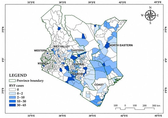
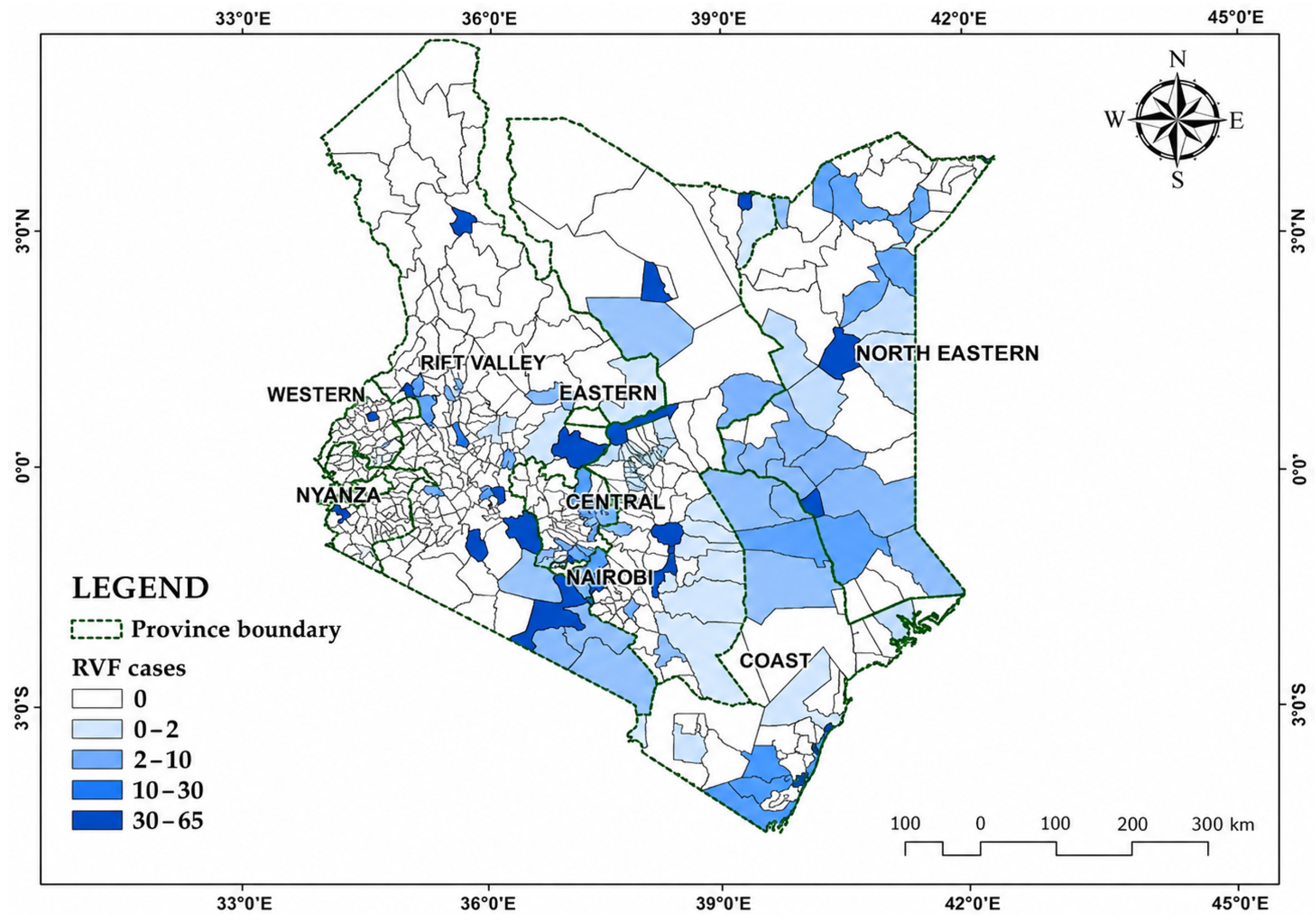
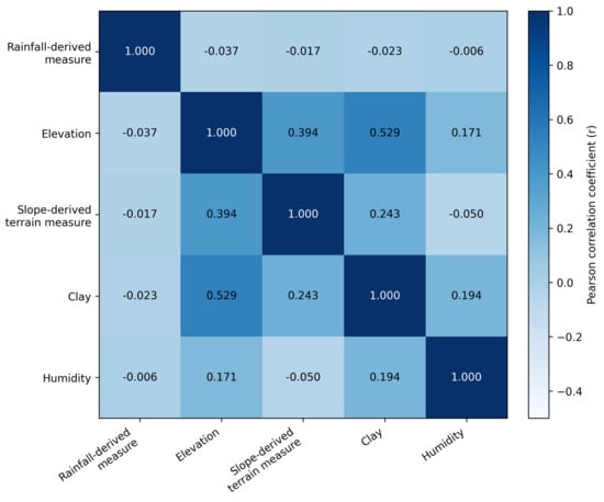
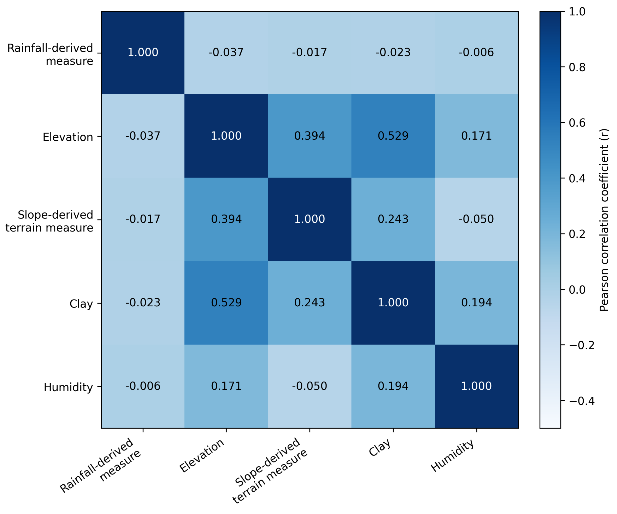
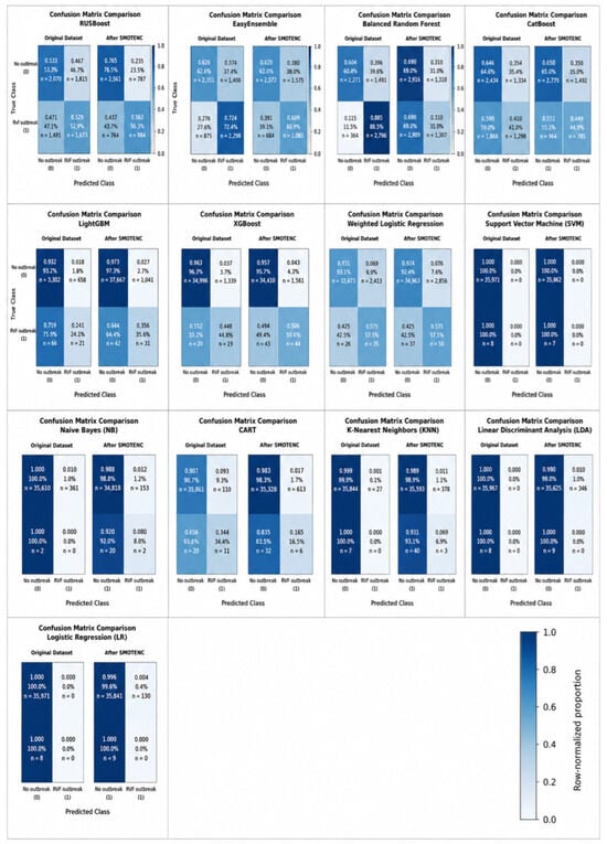
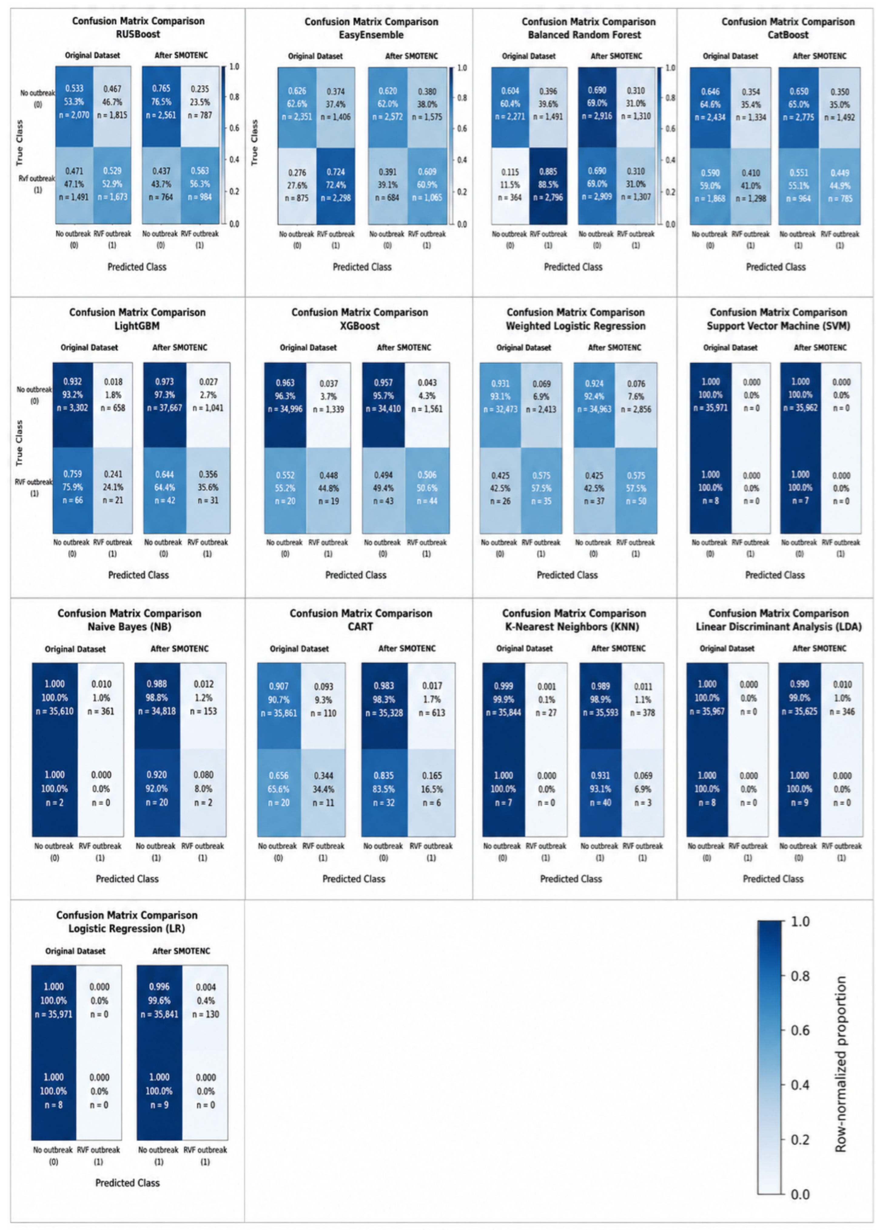
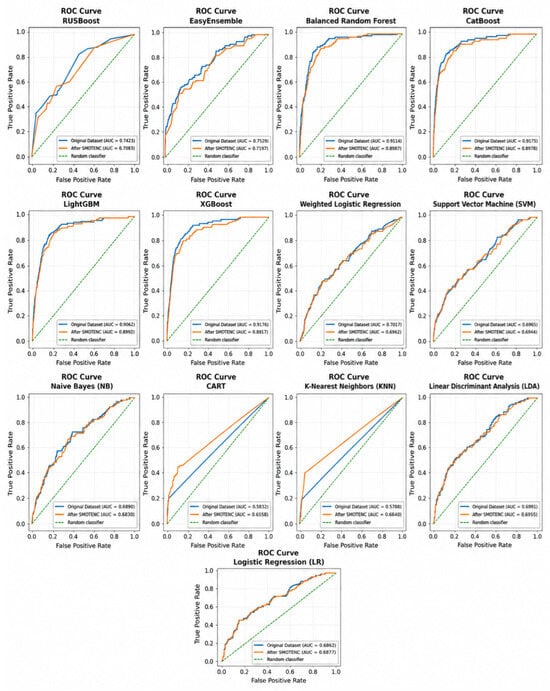
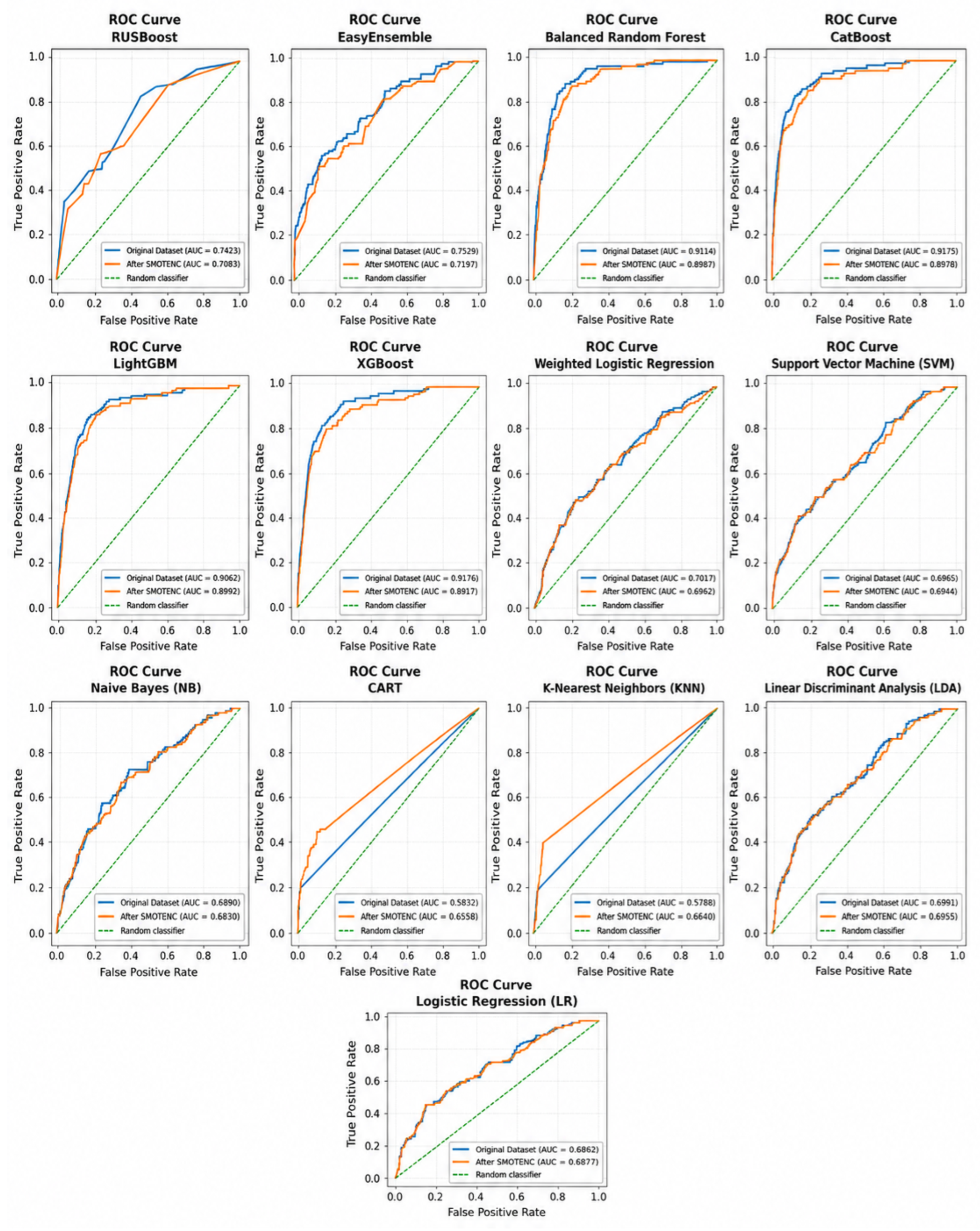
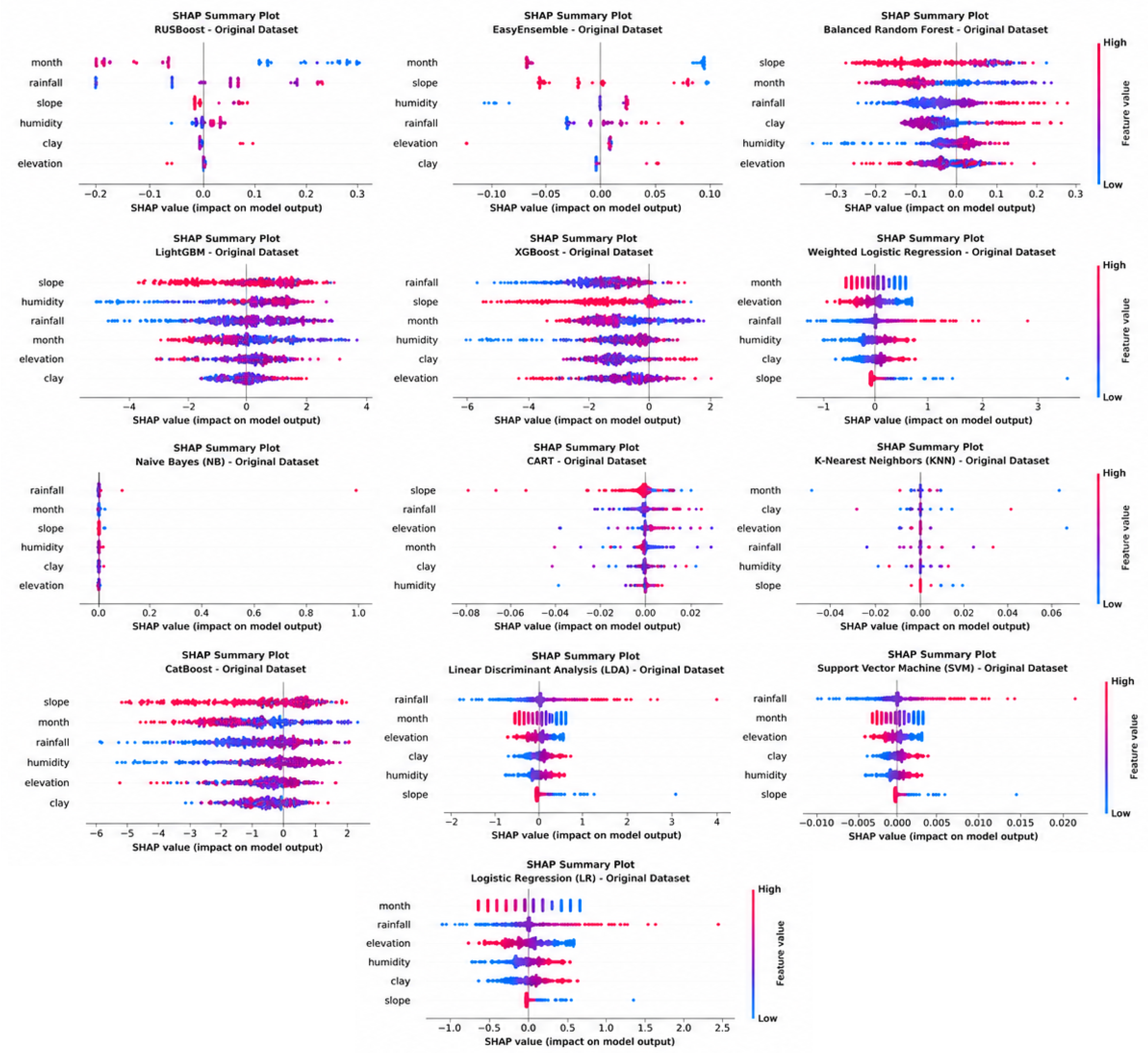
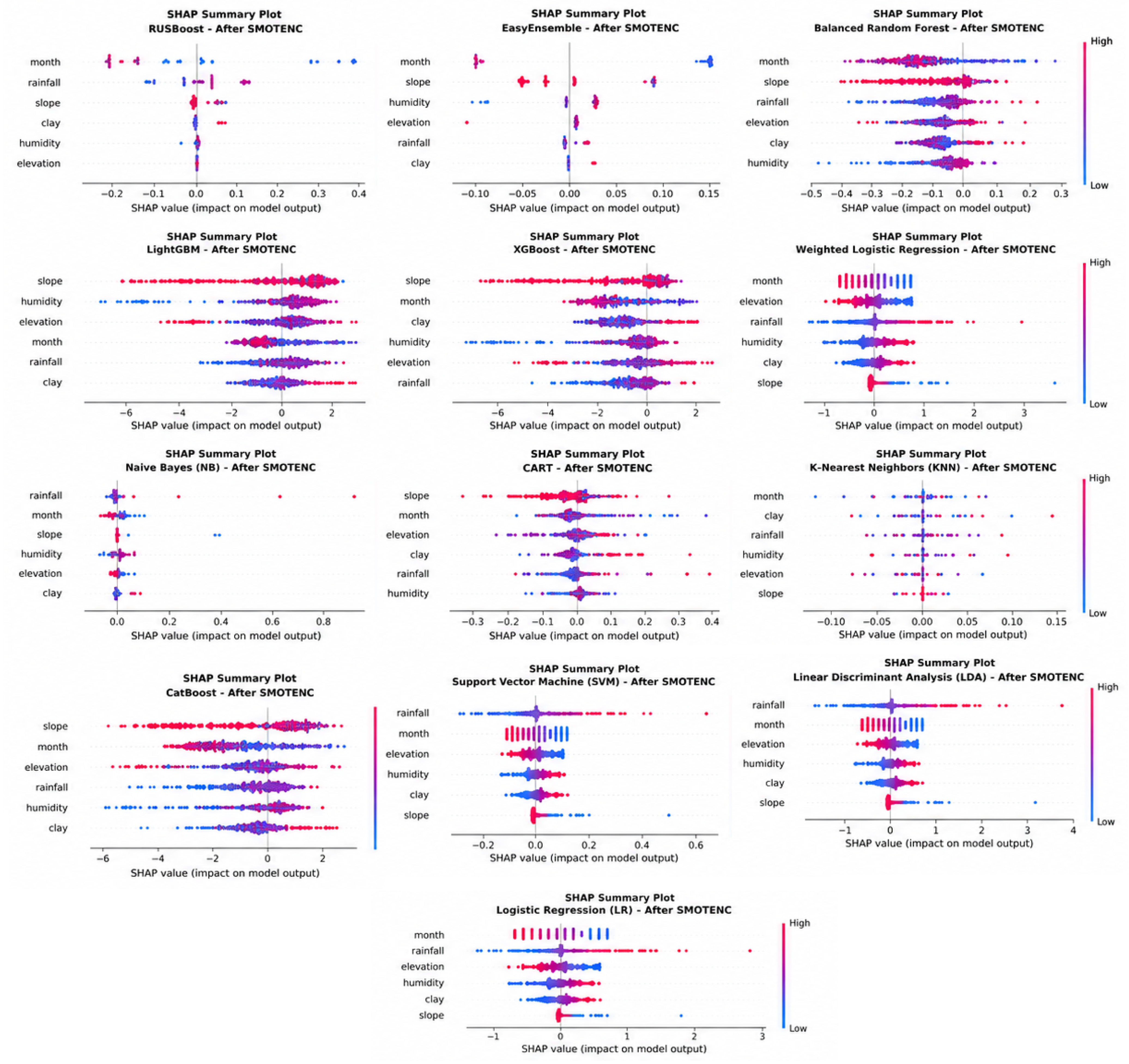
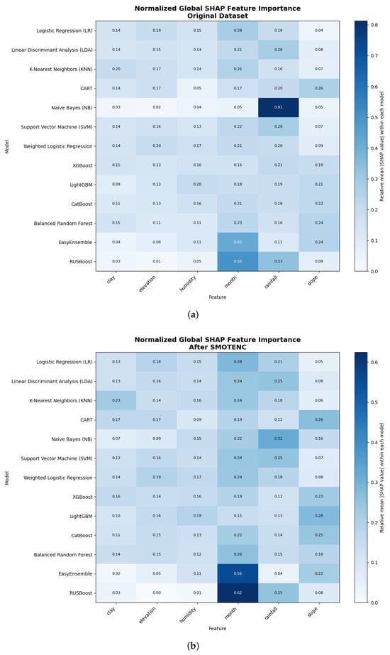

Disclaimer/Publisher’s Note: The statements, opinions and data contained in all publications are solely those of the individual author(s) and contributor(s) and not of MDPI and/or the editor(s). MDPI and/or the editor(s) disclaim responsibility for any injury to people or property resulting from any ideas, methods, instructions or products referred to in the content. |
© 2026 by the authors. Licensee MDPI, Basel, Switzerland. This article is an open access article distributed under the terms and conditions of the Creative Commons Attribution (CC BY) license.