A Regime-Adaptive Expert System for Cryptocurrency Portfolio Optimisation Using Dynamic Correlation Graph Neural Networks

Abstract

Background: Cryptocurrency allocation tools that use graph learning are often judged on gross performance and rarely stress-tested under realistic trading frictions. Methods: We evaluate a regime-supervised graph-neural tangency pipeline on 33 large-cap Binance USDT pairs (April 2021–June 2026), combining rolling Pearson correlation graphs, GCN/GraphSAGE/GAT inference under a composite Sharpe–modularity–ranking loss, and a hidden Markov layer that gates graph sparsity and long-only constraints. Six classical benchmarks share the same five-day calendar and ten-basis-point costs. An in-sample Kupiec coverage check is reported only as a diagnostic identity and is not treated as out-of-sample VaR validation. The contribution is an empirical stress test under trading frictions, not a new learning architecture: unconstrained dynamic graphs destroy net performance after costs; on this sample, a matched hidden-Markov supervisor records a higher net Sharpe ratio than a volatility-threshold rule, a descriptive difference that is not tested for significance; and no graph specification ranks above passive benchmarks on full-sample headline metrics. Results: Unconstrained dynamic graphs raise turnover by about 67% and produce negative net Sharpe; static GCN records the best GNN Sharpe (0.31), while HMM-gated GraphSAGE recovers a positive dynamic Sharpe (0.18). On this sample, cap-weight and minimum-variance rules rank above every GNN specification on headline Sharpe and drawdown; in the ablation, the HMM supervisor records a net Sharpe of 0.18 against $-0.09$ for a matched volatility-threshold rule on this sample, with no formal significance test. Conclusions: Graph adaptivity is not free. Regime supervision is associated with stronger dynamic performance in the 2023 recovery and 2024 bull windows and with weaker performance in 2022 and 2025–26. The evidence supports a sample-specific risk-policy evaluation, not an unconditional alpha claim or a practically viable allocator: positive Sharpe ratios coexist with maximum drawdowns of $-82\%$ to $-99\%$.

1. Introduction

Cryptocurrency markets now support continuous trading of a multi-trillion-dollar asset class on venues such as Binance. Institutional allocators increasingly ask for systematic portfolio tools that operate on exchange-reported prices and volumes, respond to structural breaks—the Terra/LUNA collapse of May 2022 and the FTX insolvency of November 2022 being canonical examples—and remain usable when returns are heavy-tailed [1,2]. Classical mean–variance theory, and the tangency portfolio that maximises the Sharpe ratio in particular, remains a natural benchmark for that task. In practice, however, the tangency weight $w_t\propto {\Sigma }_t^{-1}{\mu }_t$ is among the most estimation-error-sensitive objects on the efficient frontier: errors in expected returns and in the covariance matrix compound through inversion [3,4,5]. In crypto markets the problem is amplified by non-stationarity, correlation breakdown during systemic stress, and the absence of a regulated equity-style benchmark with fixed constituents.

Graph neural networks offer a structured way to share statistical strength across assets. Message-passing layers propagate information over a neighbourhood defined by an adjacency matrix, which can stabilise both mean and covariance estimates relative to asset-by-asset estimation [6,7,8]. Liu et al. [9] apply this idea to tangency portfolios, combining GCN layers with a composite loss that rewards Sharpe ratio, modularity of the estimated precision matrix, and ranking consistency. Their empirical work rests on a static industry-chain adjacency constructed from proprietary supply–demand data for CSI300 equities. The framework is persuasive for equities, yet three obstacles block a direct transfer to digital-asset management. First, tokens do not inherit corporate supply-chain graphs; value derives from protocol utility, network effects and speculative demand. Second, crypto pairwise correlations can converge toward unity in stress episodes, so a fixed topology is least informative precisely when diversification is most needed [10]. Third, classroom and prototype replications that swap industry-chain graphs for correlation graphs have rarely reported turnover, effective leverage under dollar-neutral decompositions, or drawdown decompositions, even when Sharpe ratios look acceptable alongside maximum drawdowns beyond $-85\%$.

This paper evaluates a regime-supervised graph-neural tangency pipeline for cryptocurrency portfolios on Binance USDT daily data for 33 large-cap coins through June 2026. Relative to recent GNN and network portfolio work [11,12,13,14], the contribution is not a new learning principle but an integrated empirical stress test under frictions that those studies often omit. Five components are examined together: (i) rolling correlation-graph construction; (ii) a GNN tangency engine; (iii) an HMM supervisory controller; (iv) regime-dependent sparsity and long-only rules; and (v) cost-aware execution with an in-sample Kupiec coverage check. Rolling Pearson networks replace proprietary industry-chain priors; on-chain CoinGecko attributes enrich node features.

Table 1 situates the design against nearby studies. The comparators were chosen because each is a direct predecessor on one dimension of the design: Liu et al. for GNN tangency estimation, Soleymani and Paquet for graph-based portfolio learning, Giudici and Pagnottoni for network crypto allocation, Korangi et al. for time-varying graph portfolios, and Zhou et al. for evolving graph models in crypto markets. The table is a positioning device, not a claim that ticking more boxes constitutes a new method. Jing and Rocha [15] and Ekmekcioğlu and Pınar [16] are discussed in the related-work section as further network and GNN portfolio benchmarks. The scientific spine is threefold and falsifiable: unconstrained dynamic graphs destroy net Sharpe after costs; a matched HMM-versus-volatility ablation describes how the two supervisors differ on this sample; and classical benchmarks remain stronger on full-sample headline metrics. Expert-system terminology and a design–development–testing–evaluation (DDTE) checklist are used only as documentation aids, not as claims of architectural novelty.

Table 1. Positioning relative to closest relational-portfolio and GNN tangency studies.

Study	Crypto	Dyn. Graph	Tx Costs	Class. Bench.	Regime Ctrl	Cost-Aware
Liu et al. (2026) [9]	No	Industry (static)	No	Limited	No	No
Soleymani and Paquet (2021) [17]	Yes	Learned	Partial	RL	No	Partial
Giudici and Pagnottoni (2020) [11]	Yes	Network	No	MV	No	No
Korangi et al. (2024) [12]	No	Time-var.	No	MV/HRP	No	No
Zhou et al. (2025) [13]	Yes	Evolving	No	GARCH	No	No
This paper	Yes	Roll. $\widehat{\rho }$	Yes	Six	HMM	Yes

Abbreviations: Dyn. = dynamic; Tx = transaction; Class. bench. = classical benchmarks; Regime ctrl = regime control with ablation where marked HMM; Cost-aware = net-of-cost evaluation under a stated tariff; MV = mean–variance; RL = reinforcement-learning baselines; HRP = hierarchical risk parity.

The contribution is therefore empirical and methodological rather than promotional. First, we transfer Liu-style GNN tangency estimation to exchange-native crypto data when no industry graph exists. Second, we show—with classical benchmarks—that unconstrained graph adaptivity destroys net performance after realistic turnover costs, while static and regime-supervised variants remain comparatively viable among GNN designs. Third, ablation evidence compares the HMM supervisor against a rolling-volatility threshold rule with identical decision logic; the comparison is descriptive and specific to this sample. Fourth, we report a negative result on the adaptivity hypothesis itself (H1), which prior dynamic-graph studies rarely test under identical cost conventions.

Three research questions organise the empirical design. RQ1: Can rolling correlation graphs substitute for industry-chain priors in GNN tangency estimation on exchange-native crypto data? RQ2: Does graph adaptivity improve net risk-adjusted performance once transaction costs and conventional portfolio benchmarks are applied? RQ3: Can a hidden Markov supervisory layer raise the net Sharpe of an otherwise loss-making dynamic graph strategy above zero on this sample? Five testable hypotheses follow, and Section 4 reports a verdict on each.

H1. 

Dynamic graphs raise net Sharpe relative to static graphs.

H2. 

GraphSAGE outperforms GCN and GAT among unconstrained dynamic specifications.

H3. 

Dynamic graphs increase average turnover by at least 30% relative to static graphs.

H4. 

Dollar-neutral tangency weights amplify maximum drawdown relative to long-only counterparts through gross leverage near two.

H5. 

An HMM overlay raises the net Sharpe of dynamic GraphSAGE above zero and improves calm-market performance relative to the unconstrained dynamic baseline.

The remainder of the paper is organised as follows. Section 2 reviews related work and states the novelty gap. Section 3 describes data, graph construction, GNN training, the HMM overlay and the DDTE protocol. Section 4 reports out-of-sample results. Section 5 discusses implications. Section 6 concludes. Section 7 collects limitations and future research.

2. Related Work

The problem sits at the intersection of portfolio econometrics and relational machine learning. Classical mean–variance tangency portfolios are fragile under estimation error [4,5]; shrinkage and factor structure partially stabilise inputs [18,19]; and dynamic correlation models show that dependence evolves through time [10]. Financial-network studies further demonstrate that asset relationships carry state information [20,21]. Graph neural networks now provide a learnable representation of such relationships [6,7,8], and portfolio applications are emerging in applied AI and FinTech venues [11,12,17].

For cryptocurrencies, factor structure and connectedness are well documented [2,22,23], and graph-based forecasting and allocation have advanced rapidly [11,12,13,14]. Two further anchors matter for the present design. Jing and Rocha [15] build cryptocurrency portfolios from price-correlation networks and show that network structure can change Markowitz allocations, without graph-neural estimation or transaction-cost accounting. Ekmekcioğlu and Pınar [16] use graph neural networks to stabilise deep portfolio optimisation, again outside a crypto exchange universe and without a regime supervisor. Recent work applies evolving and attention-based graph models to crypto volatility and portfolio selection [13,14], while equity GNN tangency studies such as Liu et al. [9] rely on proprietary industry-chain graphs. Yet prior GNN portfolio contributions rarely couple relational learning with (i) explicit transaction costs on a live exchange universe, (ii) a broad set of classical portfolio benchmarks under identical rebalancing rules, and (iii) a supervisory control layer ablated against simpler heuristics. The gap addressed here is a friction-aware empirical evaluation: documenting when graph adaptivity destroys rather than creates value, and whether latent-regime supervision improves on a transparent volatility trigger.

3. Materials and Methods

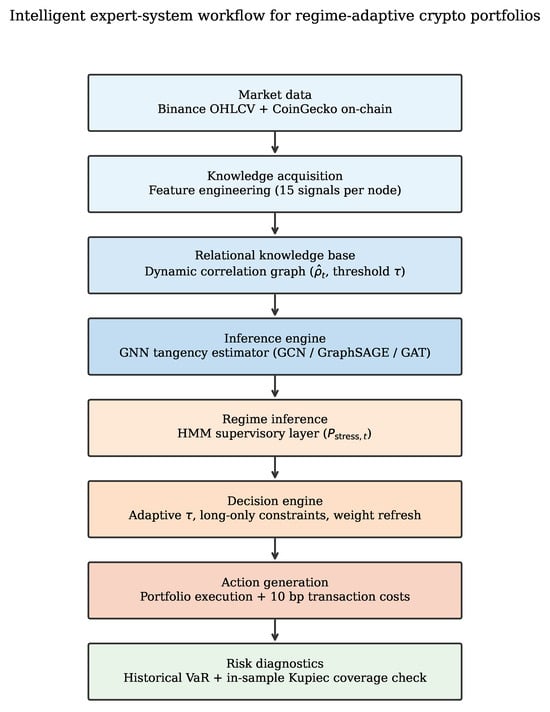
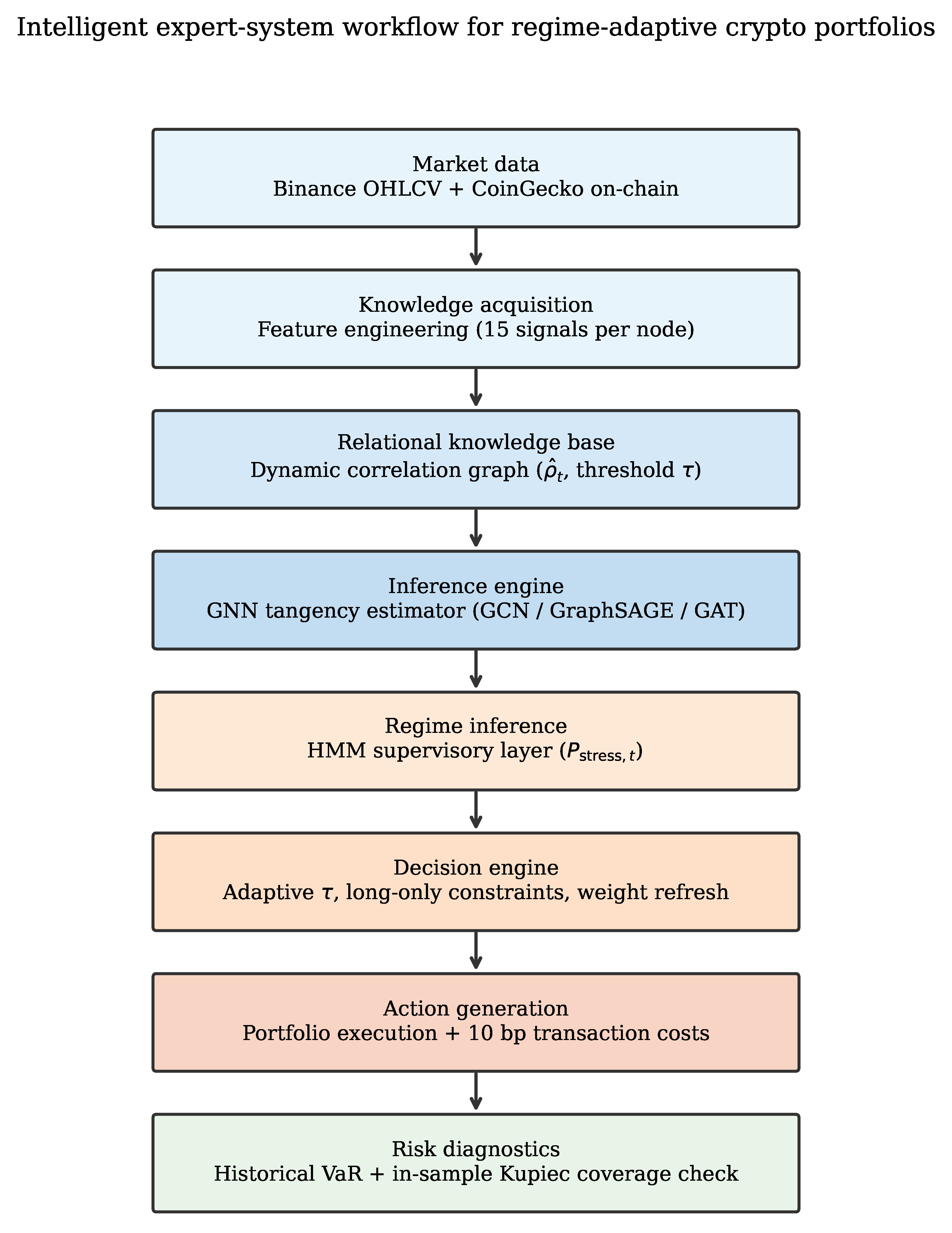
Figure 1 presents the workflow from market data to portfolio actions. Table 2 summarises the modules in decision-support terms.

Figure 1. Workflow for regime-supervised cryptocurrency portfolio evaluation. The final risk-diagnostics stage is an in-sample coverage check, not an out-of-sample VaR validation.

3.1. System Architecture

The framework implements a full decision loop rather than a standalone learner. Knowledge acquisition ingests Binance OHLCV data and CoinGecko on-chain attributes, then constructs a dynamic correlation graph whose edges encode pairwise dependence at date t. Inference is performed by the GNN tangency engine, which propagates node features over the current graph and outputs portfolio parameters through the composite loss in Equation (2). Supervisory control is provided by the HMM regime module, which infers a latent market state from benchmark return and volatility features and translates it into decision rules—raising the correlation threshold and enforcing long-only weights when stress probability is high. Action generation converts inferred weights into positions on a five-day refresh calendar and deducts ten-basis-point transaction costs. Diagnostics include an in-sample historical VaR and Kupiec [24] coverage check; as noted below, this check is not treated as out-of-sample forecast validation.

The modules are complementary rather than interchangeable. Removing dynamic graph construction leaves a static topology whose value is state-dependent (Section 3.2 and Section 4); removing the GNN engine reverts to classical mean–variance estimation without relational regularisation; removing the HMM supervisor leaves an unconstrained dynamic learner that churns excessively; and omitting cost accounting overstates net performance. Section 4 tests these design choices empirically.

3.2. Design, Development, Testing and Evaluation Protocol

To support reproducibility, we document the pipeline through a short design–development–testing–evaluation (DDTE) checklist. Table 3 maps each stage to concrete artefacts in this study. The checklist is organisational, not a claim of expert-systems novelty.

Design. Requirements were specified before estimation: exchange-native data only (no proprietary graphs), net-of-cost evaluation, leverage transparency, and falsifiable hypotheses on adaptivity (H1–H5). The knowledge base, inference engine, control layer and diagnostic module were defined with explicit inputs, outputs and failure modes (e.g., dense-graph homogeneity, Property 1; dollar-neutral leverage amplification, Property 2).

Development. Implementation uses PyTorch (v2.13.0) and PyTorch Geometric (v2.8.0.post1) for GCN, GraphSAGE and GAT; a two-state Gaussian HMM estimated with hmmlearn (v0.3.3) for regime posteriors; and a five-day rebalancing calendar with ten-basis-point turnover costs. Hyperparameters ($\tau =0.60$, 40-day graph window, 60 training epochs, composite-loss weights) were fixed ex ante from threshold-sensitivity analysis (Figure 2) and Liu et al.’s loss specification; no tuning on the July 2022–June 2026 test window was performed. Code and processed outputs are documented for replication (Data Availability Statement). Generative AI tools were used for literature organisation and code scaffolding; all numerical results and interpretations were verified by the author against the replication pipeline.

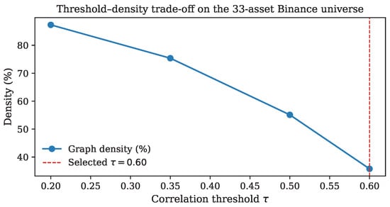
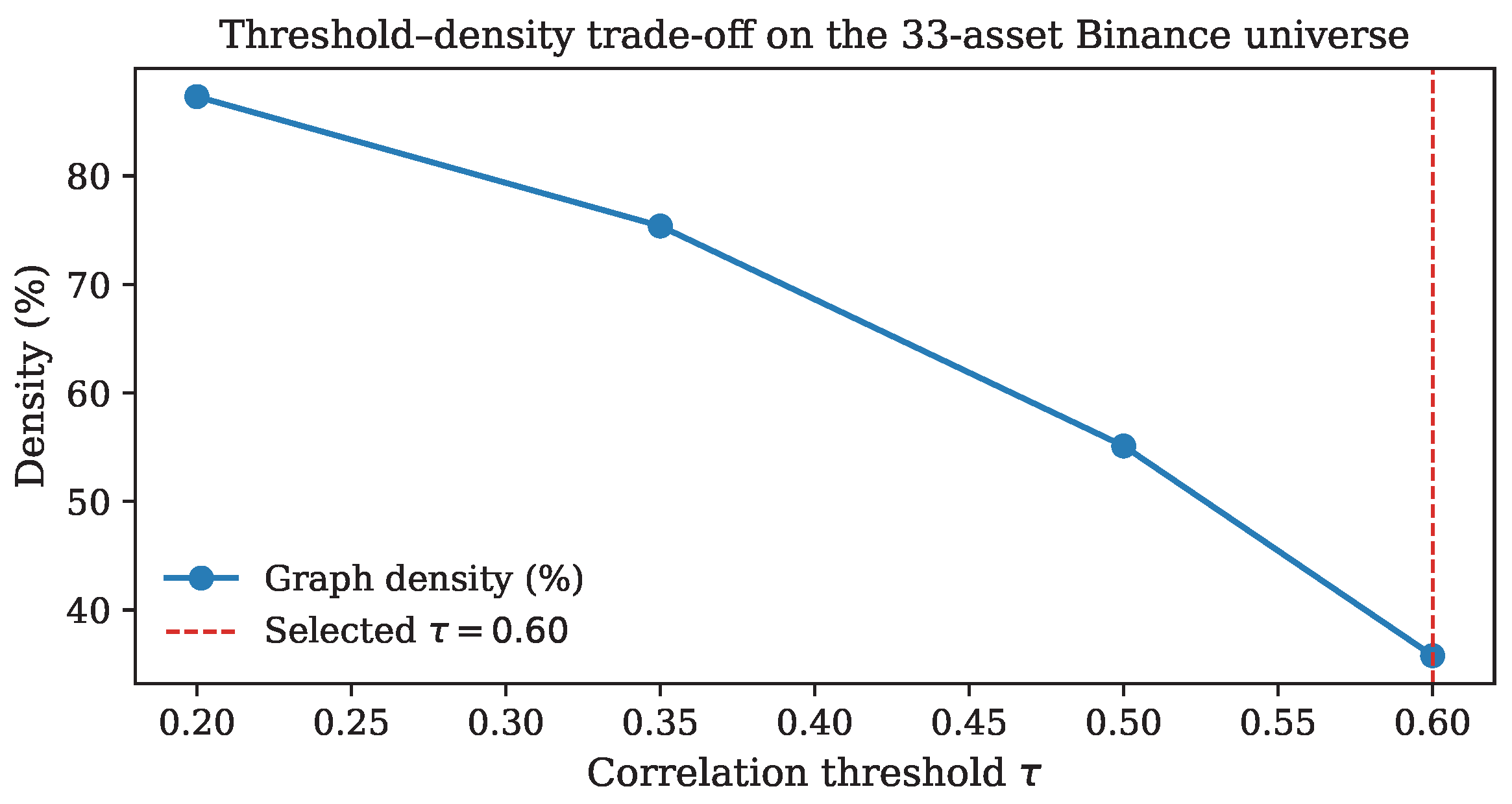
Figure 2. Correlation threshold versus graph density on the Binance universe.

Testing. Checks include an in-sample Kupiec [24] coverage identity at 5% and 1%, turnover and gross-leverage accounting, and supervisory-trigger logging (Section 4.5). Integration tests compare all GNN variants and six classical benchmarks on an identical calendar and cost convention. Ablation isolates the HMM supervisor against a volatility-rule supervisor with matched trigger thresholds.

Evaluation. Out-of-sample metrics span full-sample Sharpe, maximum drawdown, CVaR, turnover and calendar-regime splits (bear 2022, recovery 2023, bull 2024, consolidation 2025–26). Cost figures between 0 and 20 bp are obtained by linear extrapolation from gross and 10 bp net performance (not a full re-simulation). Graph-window robustness (30–50 days) and threshold sensitivity (0.20–0.60) assess density stability. Hypothesis verdicts (Section 4.2) summarise acceptance or rejection on this sample.

Table 2. Expert-system mapping for the proposed crypto tangency framework.

Module	Implementation	Role
Knowledge base	Binance OHLCV, CoinGecko on-chain scores, rolling ${\widehat{\rho }}_t$	Stores exchange-native facts and relational structure
Inference engine	PyG GCN/GraphSAGE/GAT + composite loss	Estimates tangency weights from graph embeddings
Diagnostics	Historical VaR + in-sample Kupiec check	Coverage identity check (not OOS forecast validation)
Control layer	Two-state Gaussian HMM on benchmark features	Raises $\tau$ and switches to long-only under stress

Table 2. Expert-system mapping for the proposed crypto tangency framework.

Module	Implementation	Role
Knowledge base	Binance OHLCV, CoinGecko on-chain scores, rolling ${\widehat{\rho }}_t$	Stores exchange-native facts and relational structure
Inference engine	PyG GCN/GraphSAGE/GAT + composite loss	Estimates tangency weights from graph embeddings
Diagnostics	Historical VaR + in-sample Kupiec check	Coverage identity check (not OOS forecast validation)
Control layer	Two-state Gaussian HMM on benchmark features	Raises $\tau$ and switches to long-only under stress

Table 3. DDTE protocol: stages, artefacts and evaluation criteria.

Stage	Artefact	Success Criterion
Design	Module specs, H1–H5, module map (Table 2)	All modules have defined I/O; hypotheses stated ex ante in the manuscript
Development	PyG pipeline, HMM overlay, cost engine	Reproducible run from public APIs; fixed hyperparameters
Testing	In-sample Kupiec check, ablation, trigger logs	Diagnostics logged; supervisor compared to vol. rule
Evaluation	Benchmark tables, regime splits, sensitivity	Net metrics vs. six baselines; H1–H5 verdicts

Table 3. DDTE protocol: stages, artefacts and evaluation criteria.

Stage	Artefact	Success Criterion
Design	Module specs, H1–H5, module map (Table 2)	All modules have defined I/O; hypotheses stated ex ante in the manuscript
Development	PyG pipeline, HMM overlay, cost engine	Reproducible run from public APIs; fixed hyperparameters
Testing	In-sample Kupiec check, ablation, trigger logs	Diagnostics logged; supervisor compared to vol. rule
Evaluation	Benchmark tables, regime splits, sensitivity	Net metrics vs. six baselines; H1–H5 verdicts

3.3. Data and Features

The investable universe is built from CoinGecko market-capitalisation rankings filtered to Binance USDT spot pairs with more than 95% complete daily history over April 2021–June 2026, excluding stablecoins and wrapped tokens. Membership was fixed once, using that full-sample completeness rule and a single market-cap ranking, and the same 33 names are held throughout the evaluation. The screen is therefore retrospective: coins that were delisted or too incomplete to meet the 95% threshold never enter. This survivorship filter likely flatters the level of every strategy. It does not, by itself, explain differences among strategies that share the same fixed universe. A point-in-time investable universe is not reconstructed here and is listed as a limitation. The final panel contains $n=33$ large-cap assets. Daily closes and quote-asset volumes are taken from the Binance public kline API between April 2021 and June 2026. Log returns are annualised on a 365-day convention to reflect continuous trading. A capitalisation-weighted benchmark is formed from circulating supply and Binance closes. Estimation uses data through June 2022; the out-of-sample window runs from July 2022 to June 2026 (1460 days) and spans the 2022 bear market, the 2023 recovery, the 2024 bull run and the 2025–26 consolidation.

Each node carries fifteen features. Seven exchange signals—one-, five- and twenty-day returns, twenty-day volatility, volume z-score, sixty-day momentum and RSI scaled to $[-1, 1]$—capture short-horizon price and liquidity dynamics. Eight on-chain and fundamental scores from CoinGecko—community, developer and liquidity scores, public-interest score, circulating-to-max supply ratio, and log forks, stars and four-week commits—are standardised cross-sectionally and concatenated. Where CoinGecko responses are incomplete for a subset of coins, medians fill missing cells so that the feature dimension remains balanced across the universe. These eight scores are a single cross-sectional snapshot retrieved from the CoinGecko API, not a historical panel dated to each rebalancing day. They are constant across time, so they do not import future returns into the feature path, but they can embed information that was not observable in 2021–2022. Median imputation is used only to keep the feature dimension balanced; missingness is unlikely to be random, and no separate missingness robustness check is reported. Exchange-price features, by contrast, are trailing windows ending at date t.

3.4. Dynamic Correlation Graphs and GNN Estimation

At rebalancing date t the manager seeks tangency weights

$$w_t^{\ast }={\displaystyle \frac{{\Sigma }_t^{-1}{\mu }_t}{{\mathbf{1}}^{\top }{\Sigma }_t^{-1}{\mu }_t}}.$$

(1)

Rather than estimate ${\mu }_t$ and ${\Sigma }_t$ asset by asset, we construct a graph neighbourhood and learn embeddings that pool information from correlated peers. Over a trailing forty-day window we compute the Pearson matrix ${\widehat{\rho }}_t$ and form a binary adjacency $A_{ij,t}=⊮\left(\right|{\widehat{\rho }}_{ij,t}|>\tau )$, retaining absolute correlations so that strongly anti-correlated pairs remain informative for diversification. The absolute-value rule is a modelling choice, not a claim that $+0.8$ and $-0.8$ are economically equivalent. A large negative correlation is kept because the neighbour’s return is informative for covariance estimation even when the economic relationship is a hedge. Signed or weighted edges, and rank-correlation graphs, are natural alternatives. They are not re-estimated in this revision: the archived outputs do not contain the daily weight paths required to rerun the GNN grid, and a new training pass is left as future work. Conclusions about dynamic networks should therefore be read as conditional on this binary absolute-correlation rule. The matrix is symmetrised, self-loops are removed, and the normalised adjacency feeds GNN layers. The threshold $\tau$ is not a cosmetic hyperparameter. Under mean aggregation, dense graphs drive embeddings toward homogeneity, the Gram matrix of embeddings approaches low rank, and the implied precision matrix becomes ill-conditioned.

Property 1 (Homogeneity instability).

Let $h_i,h_j\in {\mathbb{R}}^d$ be GNN embeddings for assets connected in a dense graph under mean aggregation. As graph density $\delta \to 1$, $\parallel h_i-h_j\parallel \to 0$ for all $i,j$, so that $\widehat{\Sigma }=H{H}^{\top }/d$ approaches rank one and ${\widehat{\Sigma }}^{-1}$ becomes ill-conditioned, causing tangency weights to explode.

Figure 2 confirms the practical force of this insight on our thirty-three-node universe: density falls from about 87% at $\tau =0.20$ to about 36% at $\tau =0.60$, the calm-market default used below.

Property 2 (Gross leverage bound).

Let $w=w^{+}-w^{-}$ be a dollar-neutral soft-max decomposition with ${\mathbf{1}}^{\top }{w}^{+}={\mathbf{1}}^{\top }{w}^{-}=1$. Gross exposure equals ${\parallel w\parallel }_1=2$. If both legs retain positive market beta $\beta >0$, then $\mathrm{Var}\left(R_p\right)\approx 4{\beta }^2{\sigma }_m^2$, amplifying drawdowns beyond the underlying index decline.

Property 2 explains why Sharpe ratios and maximum drawdowns can diverge sharply in long–short GNN tangency systems, and motivates the long-only and HMM-triggered constraints introduced later.

Two-layer GCN, GraphSAGE and GAT models are implemented in PyTorch Geometric with hidden width 16, embedding dimension 8 and precision-matrix rank capped at 64. Every twenty trading days the network is retrained for sixty Adam epochs at learning rate ${10}^{-3}$ with a ten-epoch linear warmup and gradient clipping at unit norm. The composite loss follows Liu et al. [9],

$$\mathcal{L}=\exp \left(-\sqrt{365}{\displaystyle \frac{{\overline{r}}_p}{{\sigma }_p}}\right)+{\lambda }_M{\mathcal{L}}_{\mathrm{mod}}+{\lambda }_R{\mathcal{L}}_{\mathrm{rank}},$$

(2)

with ${\lambda }_M=0.1$ and ${\lambda }_R=0.01$. Here ${\overline{r}}_p$ and ${\sigma }_p$ are the mean and standard deviation of in-sample portfolio returns $r_{p,t}=w^{\top }{r}_t$; ${\mathcal{L}}_{\mathrm{mod}}$ encourages community-aligned structure in the estimated precision matrix; and ${\mathcal{L}}_{\mathrm{rank}}$ aligns predicted weight ranks with realised twenty-day cross-sectional returns. Portfolio weights are refreshed every five days. Dollar-neutral long–short weights use

$$w_i^{+}={\displaystyle \frac{e^{{\tilde{w}}_i}}{{\sum }_j{e}^{{\tilde{w}}_j}}},w_i^{-}={\displaystyle \frac{e^{-{\tilde{w}}_i}}{{\sum }_j{e}^{-{\tilde{w}}_j}}},w_i=w_i^{+}-w_i^{-},$$

(3)

where $\tilde{w}={\widehat{\Sigma }}^{-1}\widehat{\mu }$; long-only portfolios truncate negative raw weights and renormalise.

The experimental grid crosses graph type (a static pre-test graph versus dynamic forty-day graphs), architecture (GCN, GraphSAGE, GAT) and constraint (dollar-neutral versus long-only), with HMM- and volatility-rule supervisory overlays on dynamic GraphSAGE. The static graph is not estimated on the full April 2021–June 2026 sample. At the first out-of-sample date (1 July 2022) the adjacency is computed from the preceding forty daily returns only, and that edge set is then held fixed. Later static-GCN retraining updates weights on trailing returns up to date t, but it does not update the correlation graph with evaluation-period pairs. The static GCN Sharpe of 0.31 is therefore an out-of-sample result with respect to graph topology. It is not a look-ahead comparator, and the rejection of H1 does not rest on future correlations. Six classical benchmarks—equal weight, cap weight, rolling mean–variance tangency, minimum variance, risk parity and hierarchical risk parity (HRP)—are rebalanced on the same five-day calendar and evaluated under identical ten-basis-point costs.

3.5. Design Choices

Several choices were fixed before the July 2022–June 2026 evaluation and were not selected by maximising test-window Sharpe. The forty-day correlation window is long enough to estimate a $33\times 33$ Pearson matrix and short enough to move; density at $\tau =0.60$ is stable near 60% for thirty-, forty- and fifty-day windows (Section 4.4), so forty days is a midpoint rather than a searched optimum. The calm-market threshold $\tau =0.60$ is the sparsest value in the reported grid (Figure 2): density falls from about 87% at $\tau =0.20$ to about 36% at $\tau =0.60$, which is the operating point suggested by the homogeneity argument in Property 1. The stress threshold $0.70$ is a one-step sparsification of that default, not a second optimised grid. Portfolio weights refresh every five days so that rebalancing is regular without daily turnover; the network is retrained every twenty days because a full sixty-epoch pass on every rebalance date is costly and because the five-day refresh still updates weights from the latest frozen model. The HMM triggers are probability conventions: $P_{\mathrm{stress},t}>0.5$ means the high-volatility state is the more probable one and raises $\tau$; $P_{\mathrm{stress},t}>0.6$ requires a clearer stress posterior before short exposure is switched off, because shutting the short leg is the more consequential action. These cutoffs were not chosen by scanning test Sharpe.

3.6. Transaction Costs, Risk Diagnostics, and Regime Overlay

Net returns deduct ten basis points per unit turnover on rebalancing days,

$$r_{p,t}^{\mathrm{net}}=r_{p,t}-0.001\times {\mathrm{TO}}_t,{\mathrm{TO}}_t=\frac{1}{2}\sum _i|w_{i,t}-w_{i,t-1}|.$$

(4)

Unless stated otherwise, Sharpe ratios, drawdowns and regime splits below are net of these costs. As a transparency diagnostic, historical VaR at $\alpha \in \{0.05, 0.01\}$ is computed as the full-sample empirical quantile of each strategy’s net return series and scored with the Kupiec unconditional coverage likelihood-ratio test [24]. Because the threshold is taken from the same series that is tested, the exercise is an in-sample coverage identity check rather than a validation of out-of-sample VaR forecasts; identical violation counts across strategies are therefore expected and are not interpreted as evidence of calibrated risk forecasts.

Regime adaptation is introduced through a two-state Gaussian HMM estimated on expanding windows of benchmark features $(r_t,{\sigma }_{5\mathrm{d}},{\sigma }_{20\mathrm{d}})$, using only observations dated t or earlier. At each estimation date the model is refit on that expanding sample and the portfolio uses the posterior probability of the high-volatility state at the sample endpoint. Because the endpoint has no later observations inside the estimation window, this endpoint posterior coincides with the filtered probability and does not use returns after the decision date. Probabilities are refreshed every five days and carried forward until the next refresh. The implementation is therefore a real-time filtered posterior, not a full-sample smoothed path. When $P_{\mathrm{stress},t}>0.5$ the correlation threshold rises from $0.60$ to $0.70$, sparsifying the graph; when $P_{\mathrm{stress},t}>0.6$ the portfolio switches to long-only weights to shut off short-leg leverage. For ablation, a volatility-rule supervisor applies the same decision logic to a normalised twenty-day benchmark-volatility score rather than an HMM posterior, allowing a descriptive comparison of latent regime inference with a transparent volatility trigger. No significance test is applied to this comparison.

4. Results

4.1. Overall Performance

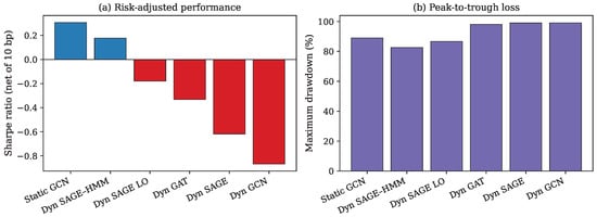
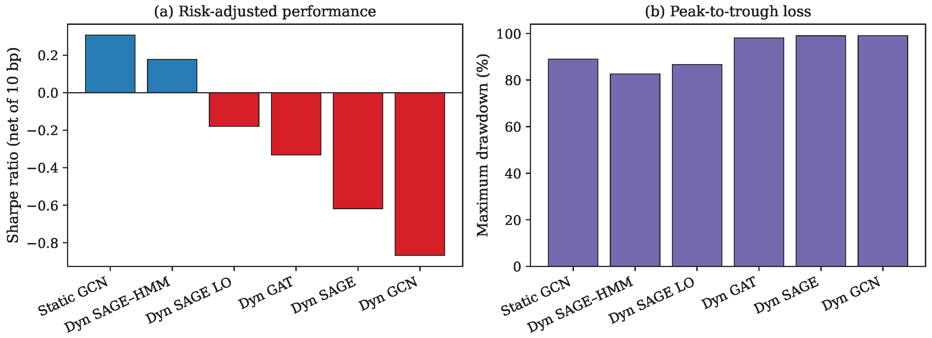
Table 4 and Figure 3 summarise out-of-sample performance after ten-basis-point costs, evaluated under the DDTE protocol of Section 3.2. The static GCN records the strongest GNN Sharpe ratio (0.31) with annualised return 22.1%. Among dynamic specifications, only the HMM-augmented GraphSAGE remains positive (Sharpe 0.18). Unconstrained dynamic GraphSAGE, GCN and GAT all deliver negative net Sharpes, despite occasional gross-of-cost improvements in prototypes without transaction costs. The ranking reverses the naive expectation that more frequent graph updates must dominate a static topology: once turnover is priced, inertia can be an advantage.

Table 4. Out-of-sample performance, July 2022–June 2026, net of 10 bp transaction costs ($n=1460$ days).

Strategy	Ann. Ret.	Ann. Vol.	Sharpe	Max. DD	CVaR95	Turnover
Static GCN	22.1%	71.7%	0.31	$-89.0\%$	$-8.5\%$	1.09
Dyn. SAGE–HMM	13.1%	73.5%	0.18	$-82.6\%$	$-8.9\%$	1.53
Dyn. SAGE long-only	$-12.0\%$	66.9%	$-0.18$	$-86.7\%$	$-8.5\%$	0.68
Dyn. GAT	$-29.4\%$	88.6%	$-0.33$	$-98.1\%$	$-11.1\%$	1.57
Dyn. SAGE	$-57.6\%$	93.2%	$-0.62$	$-99.0\%$	$-12.3\%$	1.82
Dyn. GCN	$-67.9\%$	78.2%	$-0.87$	$-99.1\%$	$-10.1\%$	1.55

Figure 3. Net-of-cost Sharpe ratios and maximum drawdowns for PyG tangency strategies, July 2022–June 2026. In panel (a), blue bars denote positive and red bars negative net Sharpe ratios. Panel (b) uses a single colour and reports maximum drawdown as a positive percentage loss. LO = long-only.

Table 5 places the GNN strategies alongside conventional rules estimated on the identical calendar and cost convention. Capitalisation-weight and rolling minimum-variance benchmarks attain higher net Sharpe ratios (0.50 and 0.45) and materially lower drawdowns ($-59\%$ and $-53\%$) than any GNN configuration over the full sample. The comparison therefore rejects a claim that graph learning ranks above passive crypto allocation on headline risk-adjusted performance in this sample. The value of the study lies instead in (i) operationalising Liu-style tangency estimation without proprietary graphs, (ii) documenting when adaptivity destroys value after costs, and (iii) showing that a regime-supervised overlay can restore positive dynamic performance in recovery and bull windows (Section 4.5).

Table 5. GNN strategies versus conventional benchmarks, July 2022–June 2026, net of 10 bp costs.

Strategy	Ann. Ret.	Ann. Vol.	Sharpe	Max. DD	Turnover
Cap-weight	24.5%	49.5%	0.50	$-59.0\%$	0.00
Min-variance	21.9%	48.5%	0.45	$-52.6\%$	0.10
Mean–variance	2.9%	61.4%	0.05	$-81.0\%$	0.16
Risk parity	1.8%	61.6%	0.03	$-78.7\%$	0.01
HRP	$-13.4\%$	66.8%	$-0.20$	$-85.0\%$	0.63
Static GCN	22.1%	71.7%	0.31	$-89.0\%$	1.09
Dyn. SAGE–HMM	13.1%	73.5%	0.18	$-82.6\%$	1.53
Equal-weight benchmark	$-2.7\%$	65.4%	$-0.04$	$-82.6\%$	0.00
Dyn. SAGE	$-57.6\%$	93.2%	$-0.62$	$-99.0\%$	1.82

The hypothesis that dynamic graphs raise Sharpe relative to static graphs is therefore rejected under full training with costs: static GCN ranks highest among GNN designs. Architecture comparisons among unconstrained dynamic models are clearer than the introductory H2 wording anticipated. GAT ($-0.33$) is less destructive than unconstrained SAGE ($-0.62$) or GCN ($-0.87$), so GraphSAGE does not win among unconstrained dynamic specifications; H2 is rejected. Only the HMM overlay restores a positive dynamic Sharpe, which is the object of H5 rather than H2.

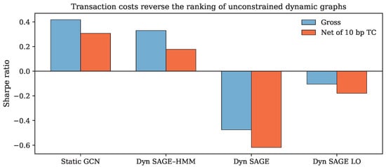
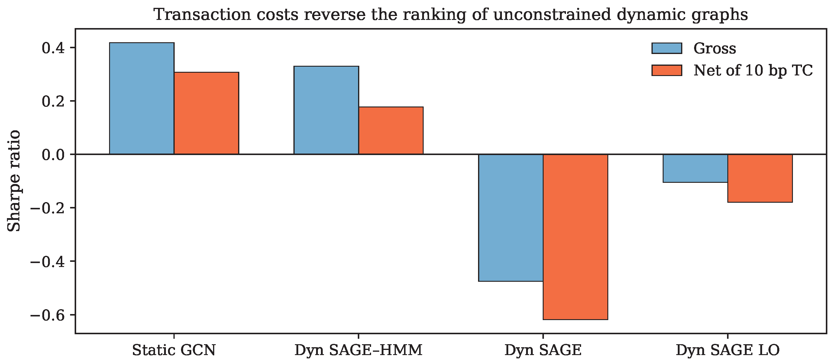
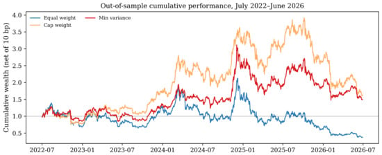
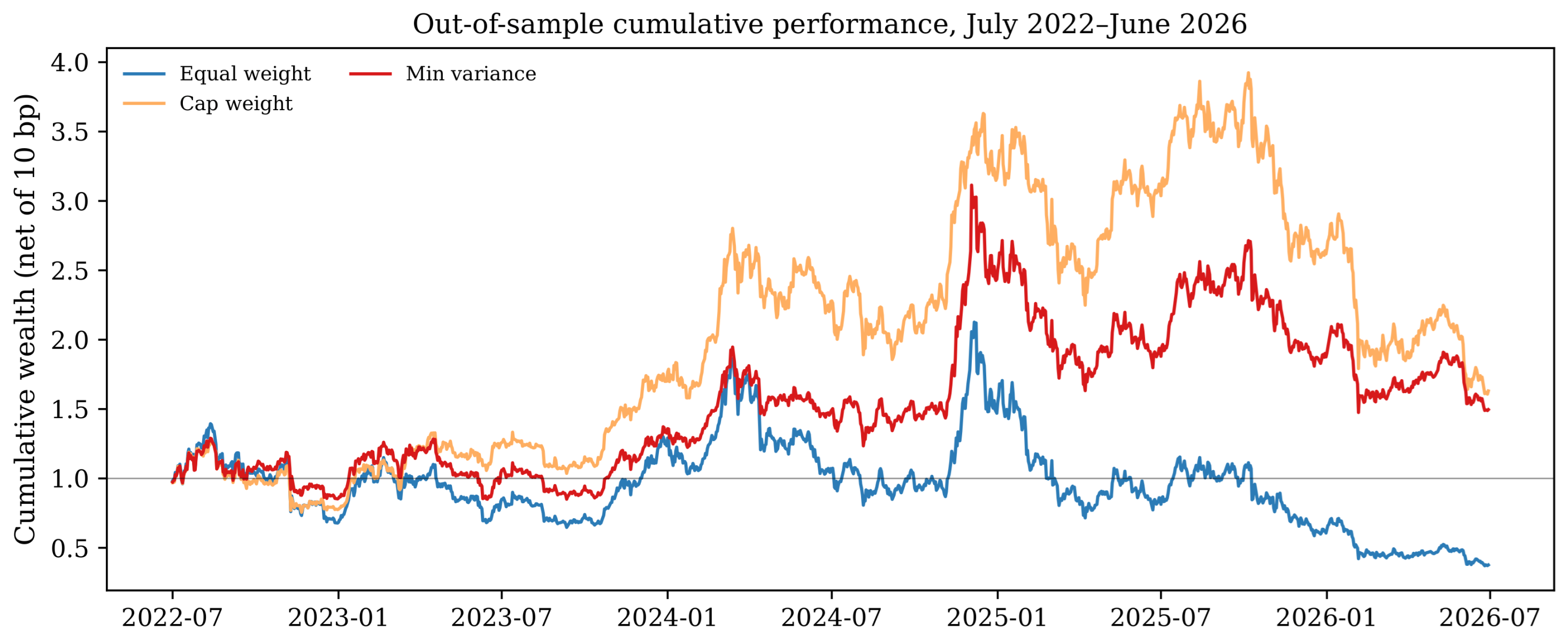
Figure 4 makes the cost channel explicit. Gross-of-cost Sharpes for dynamic GraphSAGE and the HMM overlay look more competitive; after ten basis points the unconstrained dynamic strategy collapses, while the static GCN retains a clear lead. Any evaluation that reports only gross performance would therefore overstate the case for unconstrained adaptivity. Figure 5 plots cumulative wealth for the equal-weight, cap-weight and minimum-variance benchmarks. GNN wealth paths are not plotted because their daily return series were not archived (Section 7); GNN performance is reported in Table 4 and, by calendar window, in Section 4.5.

Figure 4. Gross versus net-of-cost Sharpe ratios for selected strategies.

Figure 5. Cumulative wealth of the equal-weight, cap-weight and minimum-variance benchmarks, net of 10 bp transaction costs, July 2022–June 2026. The grey horizontal line marks initial wealth of 1.

4.2. Risk Diagnostics and Turnover

Table 6 reports the in-sample Kupiec coverage identity check on net returns. Violation counts match $n\alpha$ at both the 5% and 1% levels for the tabulated strategies, and p-values fail to reject correct unconditional coverage—as expected when VaR is the full-sample empirical quantile of the same series. Extreme drawdowns therefore coexist with a mechanically non-rejected coverage identity: the check does not establish calibrated out-of-sample risk forecasts, and it is not used as a contribution claim.

Table 6. In-sample Kupiec [24] coverage identity check on net-of-cost returns (full-sample historical VaR).

Strategy	$\mathit{\alpha }$	Violations	Expected	LRuc	p-Value
Static GCN	5%	73	73.0	0.00	1.00
Static GCN	1%	15	14.6	0.01	1.00
Dyn. SAGE–HMM	5%	73	73.0	0.00	1.00
Dyn. SAGE–HMM	1%	15	14.6	0.01	1.00
Dyn. SAGE	5%	73	73.0	0.00	1.00
Dyn. SAGE	1%	15	14.6	0.01	1.00

Turnover and leverage clarify the cost channel (Table 7). Dynamic GraphSAGE turns over 1.82 on average, about 67% above the static GCN (1.09), supporting H3. At ten basis points, that gap is large enough to convert a weak gross outcome into a clearly negative net Sharpe. Dollar-neutral GNN portfolios operate near gross leverage of two; the long-only GraphSAGE cuts leverage to one and turnover to 0.68, improving drawdown relative to unconstrained SAGE while remaining short of the static GCN on risk-adjusted return. The leverage-amplification hypothesis (H4) is supported in direction—drawdowns deepen under dollar-neutral weights—even though the drawdown ratio versus long-only falls slightly below a strict 1.5 threshold.

Table 7. Average turnover and gross leverage for PyG strategies.

Strategy	Avg. Turnover	Gross Leverage	vs. Static
Dyn. SAGE	1.82	2.00	$+67\%$
Dyn. SAGE–HMM	1.53	1.71	$+40\%$
Dyn. GCN	1.55	1.96	$+42\%$
Static GCN	1.09	1.96	—
Dyn. SAGE long-only	0.68	1.00	$-38\%$

Note: “vs. Static” is the percentage difference in average turnover relative to static GCN; — marks static GCN as the reference row.

Table 8 summarises the hypothesis verdicts on this sample. H1 is rejected: static GCN ranks above dynamic GCN/SAGE/GAT after costs. H2 is rejected: among unconstrained dynamic models, GAT is least negative and GraphSAGE does not outperform GCN or GAT. H3, H4 and H5 are not accepted as formal tests. No block-bootstrap or other confidence interval for Sharpe differences is reported, because the archived replication files contain summary metrics rather than the daily GNN return paths required for resampling. H3 is descriptively consistent with the pre-specified turnover gap. H4 is only partly consistent with a strict drawdown-amplification threshold. H5 is descriptively consistent with the data: the HMM overlay raises dynamic-SAGE net Sharpe from $-0.62$ to $0.18$ and improves calm-market performance (Section 4.5). These are observed differences on one path, not significance claims.

Table 8. Hypothesis evaluation summary (net of 10 bp costs).

ID	Verdict	Key Evidence
H1	Reject	Static GCN Sharpe 0.31 vs. dyn. GCN $-0.87$
H2	Reject	Unconstrained ranking GAT > SAGE > GCN; HMM evidence is H5
H3	Descriptive	Turnover 1.82 vs. 1.09 ($+67\%$ vs. static)
H4	Partial	Gross leverage $\approx 2$; drawdown ratio $<1.5$
H5	Descriptive	Sharpe $-0.62\to 0.18$; calm-state gain (vol. rule $-0.09$)

Note: “Descriptive” means an observed difference on one sample path; no significance test is reported, including for the HMM versus volatility-rule comparison.

Table 9 reports a linear cost extrapolation for the leading GNN specifications. Under that extrapolation, rankings among GNN designs are unchanged between five and twenty basis points: static GCN remains the best GNN, unconstrained dynamic SAGE remains negative, and the HMM overlay preserves a positive but modest Sharpe. The cap-weight benchmark continues to rank highest on headline Sharpe at higher cost assumptions because its turnover is negligible. These figures are not a full re-simulation of alternative cost paths.

Table 9. Illustrative linear cost sensitivity of Sharpe ratios. Rows are extrapolated from gross and 10 bp net performance; they are not a full re-simulation of the weight path.

Strategy	0 bp	5 bp	10 bp	20 bp
Cap-weight benchmark	0.50	0.50	0.50	0.50
Static GCN	0.42	0.36	0.31	0.20
Dyn. SAGE–HMM	0.33	0.25	0.18	0.03
Dyn. SAGE	$-0.48$	$-0.55$	$-0.62$	$-0.76$

Note: This table is an illustrative sensitivity, not a re-estimated robustness exercise. Crypto trading costs also depend on spreads and size; that nonlinearity is not modelled here. GNN cost rows are extrapolated from gross and net performance at ten basis points; benchmark turnover is near zero.

4.3. Supervisory Overlay Ablation

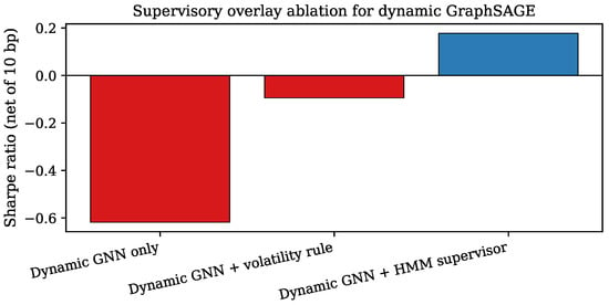
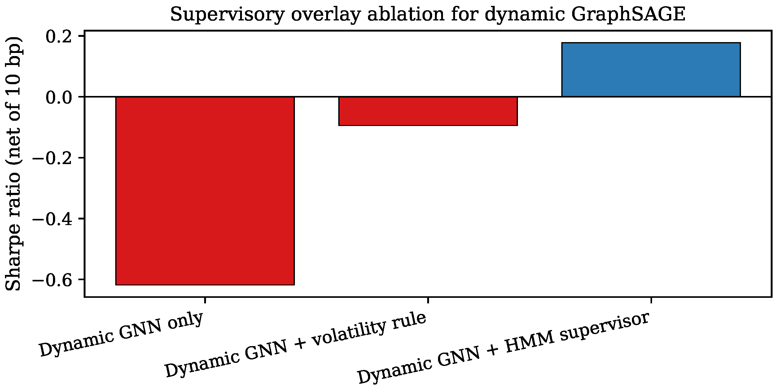
A central design question is whether the HMM supervisor is essential or whether a simpler volatility rule suffices. We therefore compare three dynamic GraphSAGE specifications that share identical graph construction, training and cost assumptions: (i) unconstrained dynamic GNN; (ii) dynamic GNN with a rolling-volatility supervisor that applies the same $\tau$ and long-only triggers to a normalised twenty-day benchmark-volatility score; and (iii) dynamic GNN with the HMM supervisor. Table 10 and Figure 6 report the results. The unconstrained dynamic model is decisively negative (Sharpe $-0.62$). The volatility rule materially reduces losses relative to the unconstrained baseline (Sharpe $-0.09$) but remains negative on a full-sample net basis, whereas the HMM supervisor is the only overlay that restores a positive Sharpe (0.18) while lowering turnover and maximum drawdown relative to both alternatives. These are point estimates from a single sample path. Because the daily return paths needed for resampling were not archived, no significance test is reported for the HMM–volatility gap. The ranking is therefore descriptive and sample-specific; it does not establish that the HMM supervisor is statistically superior to the volatility rule.

Table 10. Supervisory overlay ablation for dynamic GraphSAGE, net of 10 bp costs. Point estimates on one sample path; no significance test.

Specification	Sharpe	Max. DD	Turnover
Dynamic GNN only	$-0.62$	$-99.0\%$	1.82
Dynamic GNN + volatility rule	$-0.09$	$-95.4\%$	1.59
Dynamic GNN + HMM supervisor	0.18	$-82.6\%$	1.53

Figure 6. Supervisory overlay ablation: net Sharpe ratios for dynamic GraphSAGE variants. Blue bars denote positive and red bars negative net Sharpe ratios.

4.4. Robustness and Sensitivity Analysis

Table 11 summarises robustness checks. Correlation-threshold sensitivity (Figure 2) shows that graph density falls from 87% to 36% as $\tau$ rises from 0.20 to 0.60, confirming that sparsification is materially affected by the supervisory layer’s threshold shifts. Graph-window sensitivity indicates stable average density near 60% for thirty-, forty- and fifty-day windows, suggesting that the forty-day default is not an accidental density optimum. The transaction-cost extrapolation in Table 9 preserves GNN rankings between five and twenty basis points, while passive benchmarks with negligible turnover remain strongest on headline Sharpe throughout.

Table 11. Sensitivity analysis summary.

Parameter	Range Tested	Main Finding
Correlation threshold $\tau$	0.20–0.60	Density 87% → 36%; HMM shifts 0.60 → 0.70
Graph rolling window	30, 40, 50 days	Density stable near 60% at $\tau =0.60$
Transaction cost	0–20 bp (extrapolated)	Linear extrapolation preserves GNN ranking
Supervisory rule	Vol. vs. HMM	Only HMM gives positive Sharpe (descriptive)

4.5. Regime Analysis

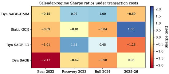
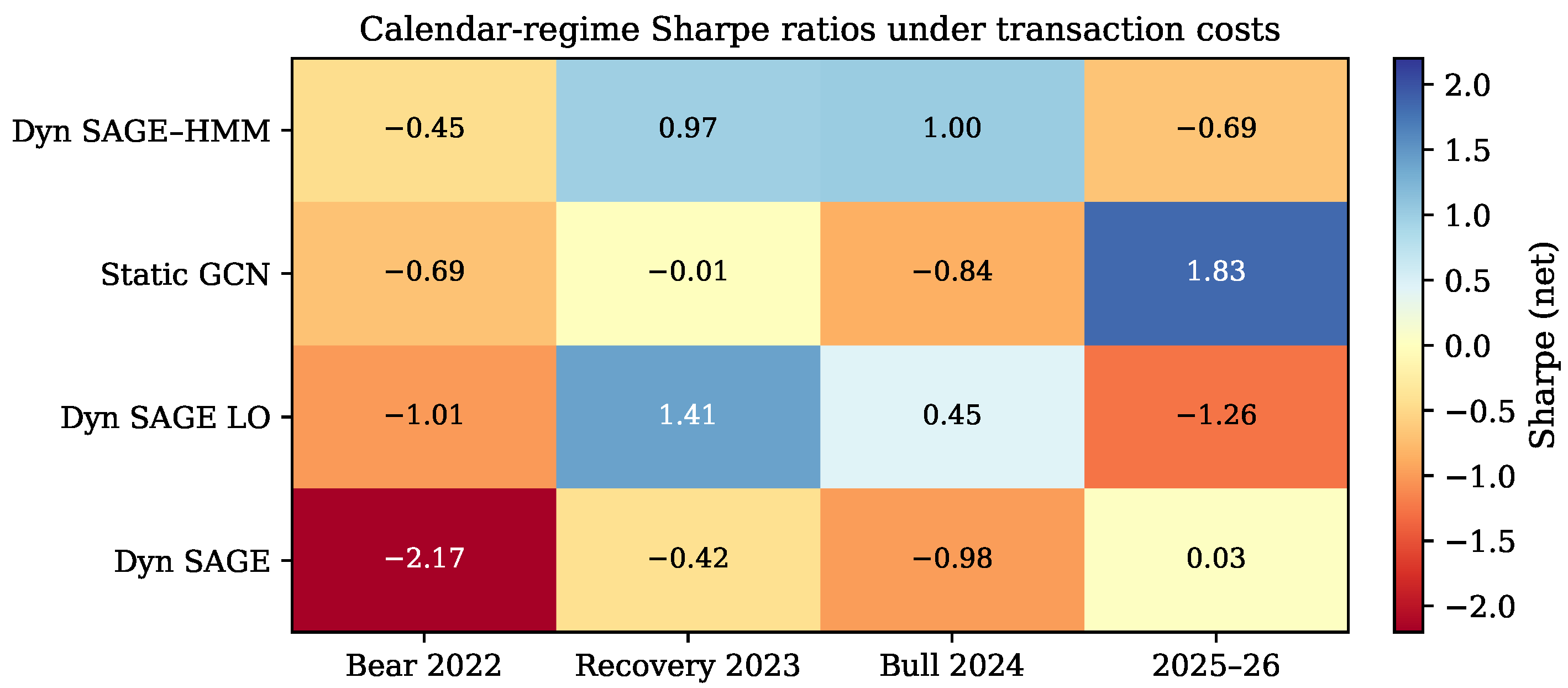
Calendar splits (Table 12 and Figure 7) show that no architecture is reliable in every state. The HMM overlay posts Sharpe ratios of 0.97 in the 2023 recovery and 1.00 in the 2024 bull market, far above unconstrained dynamic SAGE in the same windows, but the same overlay is negative in the 2022 bear window ($-0.45$) and in 2025–26 ($-0.69$). The static GCN, by contrast, is weak through 2022–24 but strong in 2025–26 (Sharpe 1.83). The useful reading is therefore not that HMM supervision restores dynamic graphs in general. It is that supervision helps in some windows and fails in others, while the frozen pre-test graph helps in a different window. No single graph rule dominates the calendar split. Long-only GraphSAGE also recovers in 2023 (1.41) but deteriorates again in 2025–26.

Table 12. Calendar-regime Sharpe ratios, net of 10 bp costs.

Strategy	Bear 2022	Recovery 2023	Bull 2024	2025–26
Dyn. SAGE–HMM	$-0.45$	0.97	1.00	$-0.69$
Static GCN	$-0.69$	$-0.01$	$-0.84$	1.83
Dyn. SAGE long-only	$-1.01$	1.41	0.45	$-1.26$
Dyn. SAGE	$-2.17$	$-0.42$	$-0.98$	0.03

Figure 7. Calendar-regime Sharpe heatmap under ten-basis-point costs.

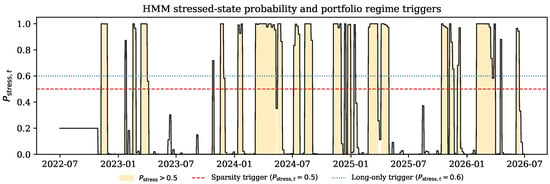
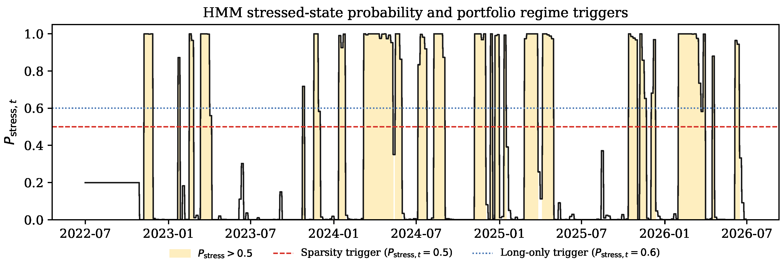
HMM-state splits reinforce the same mechanism (Table 13). Unconstrained dynamic SAGE performs relatively well in HMM stress (Sharpe 0.46) but collapses in calm markets ($-1.11$). The overlay reverses that asymmetry: calm-state Sharpe rises to 0.34 while stress-state losses remain contained ($-0.16$). Relative to unconstrained dynamic SAGE, the overlay therefore raises the full-sample net Sharpe from $-0.62$ to $0.18$ and shallows maximum drawdown from $-99.0\%$ to $-82.6\%$, which is descriptively consistent with H5 on this sample rather than a formal test of it. Figure 8 plots the stressed-state probability and the two trigger levels used in portfolio construction.

Table 13. HMM calm versus stress Sharpe ratios, net of 10 bp costs.

Strategy	Calm (${\mathit{P}}_{\mathbf{stress}}\le 0.5$)	Stress (${\mathit{P}}_{\mathbf{stress}}>0.5$)
Dyn. SAGE–HMM	0.34	$-0.16$
Static GCN	0.89	$-1.00$
Dyn. SAGE	$-1.11$	0.46
Dyn. SAGE long-only	$-0.19$	$-0.16$

Figure 8. HMM stressed-state probability with sparsity and long-only triggers. The shaded areas mark days with $P_{\mathrm{stress},t}>0.5$.

5. Discussion

The results invite reflection rather than celebration, because their most instructive feature is the disconnect between the two headline measures of performance. A strategy can post a respectable Sharpe ratio while carrying a drawdown profile that no fiduciary would tolerate, and the mechanism behind this tension is leverage. When the tangency solution is left unconstrained, the optimiser responds to the thin, unstable expected-return estimates that Michaud [4] and Best and Grauer [5] warned about by taking large offsetting long and short positions. Those positions can flatter the ratio of mean to volatility over a benign stretch while exposing the portfolio to catastrophic loss the moment the estimated relationships break down. Property 2 makes the arithmetic plain: dollar-neutral soft-max weights with unit long and short mass create roughly 200% gross exposure. In a market where most constituents share a common crypto factor, the short leg does not hedge that factor; it often reinforces losses when correlations rise. The unconstrained GraphSAGE configuration, which produced a deeply negative net Sharpe ratio in our experiments, is the clearest illustration: the model was not incapable of learning structure, but the objective, applied without leverage discipline, amplified estimation error exactly as classical theory predicts. Long-only constraints and stress-triggered long-only switches are therefore best read as leverage controls rather than as secondary robustness checks.

A second theme is the trade-off between adaptivity and turnover. The appeal of a dynamic-correlation graph model is that it should re-hedge as the dependence structure of the market evolves, and in gross terms it often does. The difficulty is that every adjustment must be paid for. Once realistic transaction costs are imposed, a portion of the informational advantage that the dynamic model earns is handed straight back to the exchange, and the residual benefit must exceed the cost of trading before adaptivity is worthwhile. This explains what might otherwise look like a paradox, namely that a static graph convolutional configuration achieved the strongest net Sharpe ratio among GNN designs in our study, ranking above its more elaborate dynamic and regime-switched cousins after costs. The static model trades less, and by trading less it keeps more of what it earns. Figure 4 shows the reversal explicitly. The finding echoes the long-standing observation that simple, stable rules are hard to beat once frictions are honestly accounted for, and it cautions against equating architectural sophistication with economic value. Adaptivity is not free, and a model that reacts to every wobble in the estimated correlation matrix will, in a market as noisy as cryptocurrency, spend heavily chasing signals that do not persist.

It is precisely this tension that motivates the hidden Markov model as a control layer rather than as a forecasting device in its own right. The HMM does not try to predict returns; it decides when the dynamic apparatus should be sparsified and when short exposure should be shut off. By inferring a latent market state and gating graph density and weight constraints accordingly, the regime filter aims to concentrate risky rewiring in the periods where re-hedging pays and to fall back on stability when it does not. The HMM-gated GraphSAGE strategy, with its positive if modest Sharpe ratio of 0.18, embodies this compromise: it is more conservative than the unconstrained optimiser and more responsive than a purely static rule in recovery and bull windows. The practical lesson is that the interesting question is often not which model is best in isolation, but which meta-level policy decides when each model should act.

Placing these findings alongside the wider literature sharpens their meaning. DeepPocket [17] and the network-Markowitz approach of Giudici and Pagnottoni [11] both report that relational information improves allocation, and our gross results are consistent with that claim. Where we differ is in insisting on a cost-aware ranking against conventional benchmarks. Once that discipline is applied, the case for unconstrained dynamic relational modelling becomes more qualified than a gross comparison would suggest. Over the full sample, cap-weight and minimum-variance rules rank above every GNN specification on net Sharpe and drawdown, a result that should be stated plainly rather than obscured. The contribution is therefore not a claim that graph tangency portfolios beat passive crypto allocation in all states of the world, but an empirical stress test that (i) transfers Liu-style estimation to exchange-native data, (ii) quantifies when adaptivity destroys value, and (iii) shows that a regime-supervised overlay can recover positive dynamic performance in selected windows.

The study carries limitations that are collected in Section 7.

What, then, should a fiduciary take from this? Not that graph neural networks are a panacea, and not that they are a distraction, but that their value is contingent on leverage limits, honest cost accounting, and regime-aware constraint policy. On this sample the GNN paths are not fiduciary-ready: drawdowns remain extreme and passive rules rank higher on headline metrics. The useful content is diagnostic—when adaptivity destroys value, and how a supervisor changes that path.

Severe maximum drawdowns ($-82\%$ to $-99\%$) must be interpreted in context. Cryptocurrency markets experienced multiple drawdowns exceeding $-70\%$ at the index level during the sample (2022 bear market, FTX contagion, 2025–26 consolidation). A long–short tangency engine operating at roughly $200\%$ gross exposure on a single crypto factor will necessarily amplify those moves. Reducing drawdown from $-99\%$ to $-82\%$ under HMM supervision is an improvement relative to the unconstrained dynamic path, not a governance success in absolute terms. A positive net Sharpe is not treated as evidence that a strategy is usable. In this paper, “usable” means only that the net Sharpe on this sample is positive. It does not mean that the path is acceptable to a fiduciary. Static GCN (Sharpe 0.31, maximum drawdown $-89\%$) and HMM–GraphSAGE (Sharpe 0.18, maximum drawdown $-82.6\%$) fail that practical test. Cap-weight and minimum-variance, with smaller though still large drawdowns, remain the stronger full-sample benchmarks. The study is therefore best read as a risk-policy evaluation—showing when to sparsify graphs, when to shut off short legs, and when dynamic adaptivity destroys value—rather than as proof that any GNN strategy is ready for unconstrained fiduciary deployment.

6. Conclusions

This paper asked whether graph neural networks that encode rolling correlation structure can improve tangency portfolios once cryptocurrency trading frictions are taken seriously. To answer it we assembled a cost-aware pipeline on a live Binance universe of 33 large-cap USDT pairs, learned node representations with GCN, GraphSAGE and GAT under the composite Sharpe–modularity–ranking loss of Liu et al. [9], and estimated tangency weights from those representations. A two-state Gaussian HMM raises the correlation threshold and switches to long-only weights under latent stress. Ten-basis-point costs are imposed throughout. An in-sample Kupiec coverage identity check is reported for transparency but is not treated as out-of-sample VaR validation.

After costs, a static graph convolutional configuration delivered the strongest GNN Sharpe ratio (0.31), ranking above the regime-gated GraphSAGE strategy at 0.18 and the unconstrained GraphSAGE optimiser at $-0.62$. Maximum drawdowns remain economically severe across GNN variants, consistent with Property 2; the HMM overlay shallows the worst dynamic-SAGE drawdown from $-99.0\%$ to $-82.6\%$, which is a relative improvement only. That HMM improvement is window-specific: Sharpe ratios of 0.97 and 1.00 in 2023 and 2024 sit next to $-0.45$ in 2022 and $-0.69$ in 2025–26, while static GCN is strongest in 2025–26. Dynamic relational learning can help in gross terms, but its net advantage is contingent on leverage discipline, cost awareness and regime-sensitive control. The matched ablation is descriptive evidence on this sample, not a formal test that the HMM supervisor outperforms the volatility rule.

The contributions are empirical. We transfer Liu-style GNN tangency estimation to exchange-native crypto data; we reject unconstrained dynamic-graph adaptivity after costs (H1) and reject the claim that GraphSAGE wins among unconstrained dynamic architectures (H2); we report that, on this path, the HMM supervisor is associated with a higher dynamic-SAGE Sharpe than both the unconstrained baseline (H5) and a matched volatility trigger, with both comparisons descriptive and untested for significance; and we state plainly that cap-weight and minimum-variance rules rank above every GNN design on full-sample headline metrics. Supervisory control can matter as much as the underlying learner, but architectural sophistication should be judged on net, benchmarked performance rather than gross appeal.

7. Limitations and Future Research

The conclusions above are bounded by the following limits. Our fifteen-dimensional feature set, while informed by the crypto factor evidence of Liu and Tsyvinski [2] and the connectedness findings of Ji et al. [22], is inevitably thinner than the firm-level panels used in equity GNN tangency studies, and richer inputs such as exchange netflows or active addresses might change the balance between static and dynamic models. The eight CoinGecko scores are a current snapshot, not point-in-time histories. Our cost assumption of ten basis points is a single point rather than a full grid. Table 9 extrapolates other tariffs; it does not reprice the stored weight path, and it ignores spread and size effects. The Binance universe is a fixed list of 33 names that satisfy a full-sample 95% completeness screen, so delisted tokens are absent and levels are likely flattered. The HMM depends on the choice of observable state variables, and a different conditioning set—for example Deribit implied volatility or stablecoin-flow imbalances—could infer different regimes. The binary absolute-correlation graph, the absence of block-bootstrap intervals, and the in-sample Kupiec identity are further limits: signed or weighted edges were not re-estimated, and daily GNN return paths were not in the archived outputs, so resampling and rolling out-of-sample VaR could not be added in this revision. Training dynamics under the composite loss produce higher turnover than lightweight prototypes, so numerical results should be read as indicative of relative behaviour on this sample rather than as forecasts.

Further work should store daily weight and return paths, re-estimate signed and weighted graphs, rebuild a point-in-time universe, replace the CoinGecko snapshot with historically dated on-chain series, reprice costs from those paths, and add block-bootstrap intervals for Sharpe differences. Network metrics computed on each window, a minimum spanning tree, multi-state HMM policies, and decentralised-exchange venues are natural extensions. None of these steps is claimed as completed here.

References

- Cont, R. Empirical properties of asset returns: Stylized facts and statistical issues. Quant. Financ. 2001, 1, 223–236. [Google Scholar] [CrossRef]
- Liu, Y.; Tsyvinski, A. Risks and returns of cryptocurrency. Rev. Financ. Stud. 2021, 34, 2689–2727. [Google Scholar] [CrossRef] [Scilit]
- Markowitz, H. Portfolio selection. J. Financ. 1952, 7, 77–91. [Google Scholar] [CrossRef] [Scilit]
- Michaud, R.O. The Markowitz optimization enigma: Is “optimized” optimal? Financ. Anal. J. 1989, 45, 31–42. [Google Scholar] [CrossRef] [Scilit]
- Best, M.J.; Grauer, R.R. On the sensitivity of mean-variance-efficient portfolios to changes in asset means: Some analytical and computational results. Rev. Financ. Stud. 1991, 4, 315–342. [Google Scholar] [CrossRef] [Scilit]
- Kipf, T.N.; Welling, M. Semi-supervised classification with graph convolutional networks. In Proceedings of the International Conference on Learning Representations, Toulon, France, 24–26 April 2017. [Google Scholar]
- Hamilton, W.L.; Ying, R.; Leskovec, J. Inductive representation learning on large graphs. Proc. Adv. Neural Inf. Process. Syst. 2017, 30, 1024–1034. [Google Scholar]
- Veličković, P.; Cucurull, G.; Casanova, A.; Romero, A.; Liò, P.; Bengio, Y. Graph attention networks. In Proceedings of the International Conference on Learning Representations, Vancouver, BC, Canada, 30 April–3 May 2018. [Google Scholar]
- Liu, B.; Li, H.; Kang, L. Tangency portfolios using graph neural networks. Neural Netw. 2026, 193, 108043. [Google Scholar] [CrossRef] [Scilit] [PubMed]
- Engle, R. Dynamic conditional correlation: A simple class of multivariate generalized autoregressive conditional heteroskedasticity models. J. Bus. Econ. Stat. 2002, 20, 339–350. [Google Scholar] [CrossRef] [Scilit]
- Giudici, P.; Pagnottoni, P. Network models to enhance automated cryptocurrency portfolio management. Front. Artif. Intell. 2020, 3, 22. [Google Scholar] [CrossRef] [Scilit] [PubMed]
- Korangi, K.; Mues, C.; Bravo, C. Large-scale time-varying portfolio optimisation using graph attention networks. arXiv 2024, arXiv:2407.15532. [Google Scholar] [CrossRef] [Scilit]
- Zhou, Y.; Xie, C.; Wang, G.J.; Gong, J.; Zhu, Y. Forecasting cryptocurrency volatility: A novel framework based on the evolving multiscale graph neural network. Financ. Innov. 2025, 11, 45. [Google Scholar] [CrossRef] [Scilit]
- Jiang, Y.; Olmo, J.; Atwi, M. Deep reinforcement learning for portfolio selection. Glob. Financ. J. 2024, 62, 101016. [Google Scholar] [CrossRef] [Scilit]
- Jing, R.; Rocha, L.E.C. A network-based strategy of price correlations for optimal cryptocurrency portfolios. Financ. Res. Lett. 2023, 58, 104503. [Google Scholar] [CrossRef] [Scilit]
- Ekmekcioğlu, Ö.; Pınar, M.Ç. Graph neural networks for deep portfolio optimization. Neural Comput. Appl. 2023, 35, 20663–20674. [Google Scholar] [CrossRef] [Scilit]
- Soleymani, F.; Paquet, E. Deep graph convolutional reinforcement learning for financial portfolio management—DeepPocket. Expert Syst. Appl. 2021, 182, 115127. [Google Scholar] [CrossRef] [Scilit]
- Ledoit, O.; Wolf, M. A well-conditioned estimator for large-dimensional covariance matrices. J. Multivar. Anal. 2004, 88, 365–411. [Google Scholar] [CrossRef] [Scilit]
- Fama, E.F.; French, K.R. Common risk factors in the returns on stocks and bonds. J. Financ. Econ. 1993, 33, 3–56. [Google Scholar] [CrossRef] [Scilit]
- Onnela, J.P.; Chakraborti, A.; Kaski, K.; Kertész, J. Dynamic asset trees and portfolio analysis. Eur. Phys. J. B 2002, 30, 285–288. [Google Scholar] [CrossRef] [Scilit]
- Billio, M.; Getmansky, M.; Lo, A.W.; Pelizzon, L. Econometric measures of connectedness and systemic risk in the finance and insurance sectors. J. Financ. Econ. 2012, 104, 535–559. [Google Scholar] [CrossRef] [Scilit]
- Ji, Q.; Bouri, E.; Gupta, R.; Roubaud, D. Network causality structures among Bitcoin and other financial assets: A directed acyclic graph approach. Q. Rev. Econ. Financ. 2018, 70, 203–213, Erratum in Q. Rev. Econ. Financ. 2021, 81, 502–503. https://doi.org/10.1016/j.qref.2020.11.007.. [Google Scholar] [CrossRef] [Scilit]
- Hotz-Behofsits, C.; Huber, F.; Zörner, T.O. Predicting crypto-currencies using sparse non-Gaussian state space models. J. Forecast. 2018, 37, 627–640. [Google Scholar] [CrossRef] [Scilit]
- Kupiec, P.H. Techniques for verifying the accuracy of risk measurement models. J. Deriv. 1995, 3, 73–84. [Google Scholar] [CrossRef] [Scilit]
Disclaimer/Publisher’s Note: The statements, opinions and data contained in all publications are solely those of the individual author(s) and contributor(s) and not of MDPI and/or the editor(s). MDPI and/or the editor(s) disclaim responsibility for any injury to people or property resulting from any ideas, methods, instructions or products referred to in the content. |
© 2026 by the author. Licensee MDPI, Basel, Switzerland. This article is an open access article distributed under the terms and conditions of the Creative Commons Attribution (CC BY) license.