


Abstract
Predictive accuracy is often treated as a sufficient condition for profitable algorithmic trading, yet whether machine learning forecasts translate into trading performance that holds up across different market regimes remains contested. This study develops and stress-tests a prediction-driven, dynamically optimized trading framework across twelve instruments spanning equities, commodities, foreign exchange, and cryptocurrencies, and three structurally distinct regimes: a calm market (2018), the COVID-19 crisis (2020), and the Russian–Ukrainian geopolitical shock (2022). Daily price forecasts from RNN, LSTM, GRU, and hybrid architectures feed a rule-based framework that opens long or short positions from the divergence between predicted and observed prices, applies volatility-adjusted stop-loss and take-profit thresholds optimized by Sharpe-ratio grid search, and is extended with a rolling-MAPE confidence filter and an error-based dynamic position-sizing rule. Across the resulting 36 asset-period combinations, the prediction-based strategies outperformed the buy-and-hold benchmark in 86–92% of cases on cumulative return and 92% of cases on the Sharpe ratio; a one-sided binomial sign test rejects the null of no systematic advantage at p < 0.001 for every strategy variant, and the pattern is stable when each of the three regimes is examined separately (10–11 of 12 assets per period). Excluding crude oil—the only instrument where active strategies persistently underperformed, plausibly reflecting structural breaks such as the negative 2020 futures prices—raises the win rate to roughly 97%. Median outperformance reached about 15 percentage points in cumulative return and close to two Sharpe-ratio points, with maximum drawdowns falling in almost every case. The rolling-MAPE filter was the most effective mechanism for containing losses in turbulent regimes, while the position-sizing variant delivered the strongest average risk-adjusted returns. These results indicate that the value of machine learning forecasts in trading depends less on raw predictive accuracy than on the risk-management logic wrapped around it, and that this advantage is statistically robust across assets, regimes, and specification choices rather than an artifact of a single favorable sample.
JEL Classification:
C32; C45; C53; E37; G17
1. Introduction
Financial market forecasting has long been regarded as one of the most complex areas of academic research, characterized simultaneously by structural uncertainty, high volatility, and nonlinear dynamics. Classical financial theories, most notably the Efficient Market Hypothesis [1], assume that asset prices follow a random walk process and that market participants are unable to systematically outperform the market over the long term. However, empirical studies conducted over the past two decades in equity, foreign exchange, commodity, and cryptocurrency markets [2,3,4,5] have identified numerous patterns and anomalies that justify the application of machine learning techniques. Parallel to the rapid advancement of artificial intelligence, an increasing number of studies have examined whether active trading strategies based on predictive models are capable of improving risk-adjusted performance and outperforming passive buy-and-hold approaches. Research on prediction-driven trading strategies has evolved along two major directions. On the one hand, deep learning models—particularly LSTM-, GRU-, and CNN-based architectures—have demonstrated a strong ability to capture hidden temporal patterns in financial time series [6,7,8,9,10,11]. On the other hand, reinforcement learning frameworks have become increasingly widespread due to their capability to continuously adapt to changing market regimes and support dynamic portfolio management [12,13,14,15]. Recent studies have further emphasized that predictive accuracy alone is insufficient for successful trading performance. The decision-making logic built upon forecasting models (filtering mechanisms, position sizing, or volatility-based risk management) plays at least as important a role as forecast accuracy itself [16,17,18,19,20]. The 2018–2022 period provides a particularly relevant framework for investigations of this kind. During this interval, financial markets experienced three distinct market regimes: (1) a relatively calm and trend-oriented environment in 2018, (2) extreme uncertainty during the COVID-19 pandemic in 2020, and (3) a high-inflation environment characterized by geopolitical shocks in 2022. These conditions create an excellent opportunity to evaluate how trading strategies derived from machine learning forecasts behave under different market regimes and whether they can provide more stable risk management than passive investment approaches. Existing literature increasingly suggests that the advantages of ML-based models become especially pronounced in highly volatile environments [21,22,23]. In cryptocurrency markets—characterized by extreme volatility and nonlinear structures—machine learning models have proven particularly effective [24,25]. In equity markets, LSTM-based approaches have shown strong performance in capturing medium-term trends, while in foreign exchange markets ML-based systems have generally generated more stable but moderate excess returns [26]. At the same time, findings across asset classes also indicate that the performance of ML models depends strongly on the structural characteristics of the underlying time series, including volatility, the frequency of regime shifts, and exposure to fundamental shocks. The aim of the present study is to develop and evaluate a prediction-driven, parameter-sensitive trading strategy across multiple financial instruments and distinct market environments. The novelty of the proposed framework lies in combining position-switching signals based on the divergence between predicted and observed prices with volatility-based stop-loss and take-profit mechanisms optimized through Sharpe ratio maximization. An enhanced version of the model additionally incorporates prediction error (MAPE) both as a filtering mechanism and as a dynamic position-sizing rule. Although such approaches remain relatively underexplored in the literature, they represent an important step toward adaptive risk-management frameworks. Beyond constructing and backtesting the strategy, the study also formally tests whether its advantage over a passive benchmark is statistically systematic, applying a battery of non-parametric tests—an omnibus Friedman test, a directional sign test, a magnitude-sensitive Wilcoxon test, and Spearman rank correlations—to the pooled results across all instruments, regimes, and strategy specifications.
Building on this motivation, the study is guided by three research questions:
- RQ1: Do prediction-driven trading strategies deliver statistically robust outperformance over a passive buy-and-hold benchmark once results are pooled across multiple assets, asset classes, and market regimes, rather than assessed instrument by instrument?
- RQ2: Does the advantage of prediction-based strategies hold consistently across structurally different regimes—a calm market, a pandemic-driven crisis, and a geopolitical shock—or is it concentrated in specific periods?
- RQ3: To what extent do risk-management overlays, namely volatility-adjusted stop-loss/take-profit rules, MAPE-based signal filtering, and error-based position sizing, contribute to performance beyond the raw predictive signal, and does this contribution vary by asset class?
The study contributes to the existing literature in several respects. First, by simultaneously analysing multiple market regimes and asset classes, it provides a comprehensive assessment of the environments in which ML-based prediction strategies perform most effectively. Second, the parameter optimization framework offers a practical and algorithmically implementable approach for improving the efficiency of prediction-driven trading systems. Third, the evaluation extends beyond conventional return and risk indicators by also considering maximum drawdown and regime-dependent stability, thereby contributing to a more robust assessment of prediction-based trading strategies. Fourth, rather than relying on descriptive comparisons alone, the study subjects the full set of results to a formal battery of non-parametric statistical tests—an omnibus Friedman test with post hoc comparisons, a sign test, a Wilcoxon signed-rank test, and Spearman rank correlations—providing, to the authors’ knowledge, one of the more statistically rigorous robustness assessments of prediction-based trading strategies across this range of asset classes and market regimes.
2. Literature Review
The application of forecasting models in trading strategies remains a relatively underexplored area; however, several studies have attempted to examine and promote their practical implementation. Most existing investigations focus primarily on equity and cryptocurrency markets, some of which are discussed in greater detail in the following section. The discussion begins with studies concentrating on equities and stock indices.
Pourahmadi et al. [27] examined stock trading models combining reinforcement learning (RL) and technical analysis while explicitly accounting for transaction costs. The authors highlighted the limitations of conventional RL models in noisy and high-dimensional stock market environments and proposed a modified Actor–Critic-based RL framework to address these issues. The main innovation of the approach lies in augmenting the actor component with three technical indicators (Relative Strength Index (RSI), Stochastic Oscillator, and Moving Average Convergence Divergence (MACD)) in order to create more realistic and efficient trading strategies. The robustness of the model was evaluated using financial data from the S&P 500 index. The results demonstrated substantial improvements compared to traditional trading strategies. The proposed model achieved an average annual return of 11.23%, compared to only 1.57% under the buy-and-hold strategy. Furthermore, the Sharpe ratio reached 0.444 for the proposed framework, significantly exceeding the 0.057 value observed for the passive benchmark. Statistical analyses confirmed that the combination of technical analysis and reinforcement learning outperformed the conventional passive investment strategy. Zhou et al. [28] experimented with the so-called IFF-DRL (Incremental Forecast Fusion—Deep Reinforcement Learning) framework, which combines incremental learning, self-supervised time-series learning, and deep reinforcement learning (DRL) to optimize financial trading. The model first forecasts OHLCV (open, high, low, close, volume) time series using the AutoConNet predictive network and subsequently combines these forecasts with actual market data to generate daily and weekly inputs for the RL framework. Experiments were conducted on stock market indices, including the Dow Jones, S&P 500, and Hang Seng Index, over the 2007–2023 period. The methodology additionally incorporates the online Elastic Weight Consolidation (EWC) algorithm to continuously update the predictive network, thereby enabling effective adaptation to changing market regimes. The empirical results were particularly remarkable for the Hang Seng Index, where annualized returns reached 103.19%, while Sharpe ratios and other risk indicators also improved substantially relative to the buy-and-hold benchmark. The study clearly demonstrated that integrating adaptive, forward-looking forecasting mechanisms into reinforcement learning frameworks can significantly improve trading performance in volatile market environments. Ju, Shen, and Ni [22] investigated whether an LSTM-based forecasting model could generate significant excess returns relative to a traditional buy-and-hold strategy. The authors conducted a backtesting-based performance evaluation on multiple U.S. equities and analysed the results using return measures, Sharpe ratios, and maximum drawdown (MDD). The trading simulation followed the buy and sell signals generated by the LSTM model and complemented them with fixed stop-loss and take-profit levels to strengthen risk management. The best performance was achieved for Tesla (TSLA), where annualized returns reached 41.26%, accompanied by a Sharpe ratio of 1.79 and a relatively limited maximum drawdown of −12.34%. For Microsoft (MSFT), the annualized return amounted to 29.47%, with a Sharpe ratio of 1.12 and a maximum drawdown of −10.51%. By contrast, the buy-and-hold strategy generated returns of only 14.85% and 12.21%, respectively, with substantially lower Sharpe ratios (TSLA: 0.58; MSFT: 0.44). The findings demonstrated that LSTM-based decision logic is not only suitable for forecasting market trends but can also deliver superior performance within active trading strategies. In addition, the LSTM-generated strategies typically exhibited smaller maximum drawdowns and more favourable return-to-risk ratios than the conventional benchmark strategy. The authors emphasized that such models may be particularly effective over medium-term horizons, where temporal patterns embedded in financial time series can be exploited more efficiently. The study therefore provided strong evidence that LSTM-based price forecasting offers not only theoretical but also practical advantages for capital market trading. Shah et al. [29] presented a stock market trading framework based on deep learning architectures designed for automated trading of the Nifty 50 index. The proposed strategy relies on a stacked CNN–LSTM model using a 20-day lookback window to analyse market data. Although the primary objective of the study was accurate price forecasting, the framework implicitly described a trading strategy built upon these predictions. Trading signals were generated according to forecasts of the Nifty 50 closing price, thereby optimizing trading decisions. The CNN–LSTM approach achieved substantially higher returns than the traditional buy-and-hold strategy, which generated a cumulative return of 107% over ten years, whereas the proposed framework achieved excess returns of 342%. Quantifying predictive outputs—the target variable of the model—may assist traders in identifying trading opportunities, particularly in the context of derivative and options markets. Cheng et al. [30] investigated a time-series framework combining deep learning with an integrated indicator-selection methodology for stock price forecasting and trading strategy development. The proposed framework follows a hybrid approach that combines the automated selection of financial technical indicators with deep learning models. A key component of the strategy lies in generating buy and sell signals based on the selected technical indicators, which directly influence trading decisions. The model was tested using Taiwanese stock market data, with particular emphasis placed on evaluating realized trading profits. Experimental results confirmed that the proposed framework was capable of generating significant trading profits. Specifically, during a 30-day testing period, the model achieved a gross return of 4.5%, compared to a 0.5% loss under the buy-and-hold strategy. The study highlighted the advantages of the synergistic integration of technical indicators and deep learning methods in developing more reliable and profitable algorithmic trading strategies.
Another popular asset class in the literature is cryptocurrencies. Several empirical studies in this area are presented below. Jing and Kang [24] introduced an automated cryptocurrency trading strategy based on an ensemble deep reinforcement learning (DRL) framework, with particular emphasis on the interpretation of visual information derived from candlestick chart images. The core idea of the strategy is that the DRL model learns complex market patterns from temporal and spatial information extracted from multi-resolution candlestick images and generates trading decisions accordingly. Model performance was evaluated using different data types and strategies over a 30-day testing period. Among the DRL-based approaches, the DQN model utilizing candlestick image (CI) data achieved the strongest performance, generating a return of 26.12% during the testing period. The corresponding Sortino ratio reached 0.0344, while the maximum drawdown remained limited to −2.10%. This strategy significantly outperformed the conventional buy-and-hold approach, which achieved an 18.54% return and a Sortino ratio of 0.02 over the same period. The study emphasized that the ensemble DRL framework, through its comprehensive use of candlestick-based visual information, provides a more sophisticated understanding of market dynamics, thereby enabling more efficient and profitable trading decisions in highly volatile cryptocurrency markets. Omole and Enke [26] applied deep learning models to forecast Bitcoin price direction and empirically compared the profitability of trading strategies built upon these predictions. The study evaluated several deep learning architectures, including CNN–LSTM, LSTM, and TCN models, against the ARIMA benchmark model using on-chain data combined with feature-selection techniques such as Boruta, genetic algorithms, and LightGBM. The trading framework generated buy and sell decisions according to predicted Bitcoin price movements. Based on the simulated trading results, the “long and short” strategy achieved the best performance, generating an annualized return of 6653.74% and a Sharpe ratio of 1.85. This substantially outperformed both the “long-only buy-and-sell” strategy (437.24% return; Sharpe ratio: 0.13) and the “short-only buy-and-sell” strategy (1084.16% return; Sharpe ratio: 0.18). The study further emphasized that deep learning models and careful feature selection are critical for navigating the highly volatile and complex cryptocurrency market environment successfully and profitably. Ghadiri and Hajizadeh [25] proposed an advanced artificial intelligence-based trading system designed specifically for highly volatile cryptocurrency markets. The authors implemented a two-stage framework: first, the XGBoost algorithm was used to identify the most informative variables from market, technical, macroeconomic, and blockchain-related data; second, a deep learning architecture integrating LSTM, BiLSTM, and GRU layers was employed to generate trading signals. The framework was tested using Bitcoin and Ethereum data over the 2017–2023 period, and the results demonstrated substantial outperformance relative to the buy-and-hold benchmark. For Bitcoin, the GRU-XGB model achieved an annualized return of 24.85% with a Sharpe ratio of 0.514, whereas the buy-and-hold strategy produced a negative return of −8.9% and a Sharpe ratio of only 0.01. For Ethereum, the LSTM-XGB model delivered particularly strong performance, achieving a 90.26% annualized return and a Sharpe ratio of 1.22. The study additionally confirmed the statistical significance of the excess performance through Wilcoxon tests, especially in the case of GRU and BiLSTM architectures. The authors emphasized the importance of blockchain-related variables and the practical advantages of deep learning frameworks, while also highlighting challenges related to overfitting, data saturation, and hyperparameter optimization. Kang, Hong, and Kim [31] investigated the effectiveness of cryptocurrency trading strategies combining deep learning-based price prediction with technical indicators. The objective of the study was to develop a decision-support framework capable of improving risk-adjusted returns across several crypto assets, including Bitcoin, Ethereum, and Ripple. The authors applied twelve different deep learning architectures, including SegRNN, Transformer, and TimesNet models, and combined them with technical indicators such as Bollinger Bands, RSI, and MACD within trading simulations. Backtesting procedures were conducted across four different time horizons (30 min, 1 h, 4 h, and daily intervals), while performance was evaluated using return measures, maximum drawdown, and Sharpe ratios. The strongest performance was achieved in the Ethereum market using a strategy that combined the TimesNet model with Bollinger Bands. This framework generated a return of 3.19%, while maintaining a maximum drawdown of −7.46% and a Sharpe ratio of 3.56, substantially exceeding the buy-and-hold benchmark values. The findings indicated that although deep learning models are capable of generating accurate forecasts independently, their integration with technical indicators further improves trading strategy effectiveness. The study particularly emphasized the practical advantages of medium-term (4 h) forecasting horizons and the synergistic application of deep learning models and technical indicators in cryptocurrency trading. Viéitez et al. [21] focused on forecasting Ethereum prices and evaluating the performance of associated investment strategies, with particular attention to the practical trading applicability of machine learning models. The authors applied several forecasting models, including LSTM, GRU, and SVM architectures, across both moderately volatile and highly volatile market periods. Trading strategies derived from these models were evaluated and compared with a passive buy-and-hold strategy using cumulative returns and Sharpe ratios. The best-performing strategy emerged during the more volatile second period and was based on an active trading framework driven by the LSTM model. During testing, the strategy operated with an exceptionally low loss ratio while generating annualized cumulative returns several times higher than the benchmark buy-and-hold strategy. In the first period, the GRU model combined with Pearson-based feature selection achieved a cumulative return of 373.4%, whereas the buy-and-hold strategy generated only 91.9% over the same interval. The results further demonstrated that the best active strategy achieved a Sharpe ratio of 1.36, substantially higher than the benchmark value of 0.52, clearly indicating a considerable improvement in risk-adjusted performance. An important contribution of the study is that machine learning models were not only capable of successfully forecasting price movements, but also of generating reliable trading strategies that significantly outperformed passive investment approaches. The results proved especially convincing during highly volatile periods, where conventional buy-and-hold strategies frequently resulted in lower returns and higher risk exposure. These findings support the conclusion that properly validated machine learning models, particularly LSTM and GRU networks, can provide a reliable foundation for cryptocurrency forecasting and trading strategy development. Most studies additionally emphasize that the reported returns are presented on a gross basis, meaning that taxes, transaction costs, and other trading-related expenses are generally not incorporated into the analysis.
3. Materials and Methods
3.1. Data
In the present study, daily prices data were examined across multiple asset categories, including equity market indices (S&P 500, DAX, Nikkei 225), commodities (crude oil, gold, and silver), cryptocurrencies (Bitcoin, Ethereum, and Litecoin), as well as major foreign exchange pairs (EUR/USD, GBP/USD, and AUD/USD). The observation window extends from 1 January 2016, to 30 June 2022. For commodity markets, futures price series were utilized in the case of crude oil, gold, and silver, while spot prices were considered for all remaining assets. The selection of the sample period is justified by two primary factors. First, it incorporates heterogeneous market conditions, including a relatively calm phase (2018), the disruption caused by the COVID-19 pandemic (2020), and the geopolitical tensions emerging in 2022. Second, given the relatively recent development of cryptocurrency markets, the availability of historical data is more limited compared to traditional financial instruments; therefore, the chosen period represents a balanced compromise that ensures comparability across asset classes. The data were collected from www.finance.yahoo.com (accessed on 1 December 2022), except for cryptocurrency prices, which were retrieved from www.coinmarketcap.com (accessed on 1 December 2022).
During the data preprocessing stage and the examination of the time series, particular attention was paid to missing observations. This issue proved especially relevant for the estimation of the correlation matrix, as the number of available data points varied across assets. To mitigate this problem, linear interpolation techniques were employed. In contrast, missing values were less problematic for the forecasting models, since each asset was analysed separately. The handling of trend and seasonal components is addressed in a later section within the context of volatility modelling. For the forecasting exercises, these components were not modelled explicitly; rather, they were captured implicitly through the pattern recognition capabilities of the applied modelling approaches. Subsequently, the dataset was partitioned into three distinct subperiods. The first subsample reflects a relatively stable economic environment, covering the period from 1 January 2016, to 30 June 2018. The second subsample spans from 1 January 2018, to 30 June 2020, and was designed to capture the effects of the COVID-19 crisis. The third subsample corresponds to another period of economic turbulence associated with the Russian–Ukrainian conflict, covering the interval from 1 January 2020, to 30 June 2022. Throughout the empirical analysis, the two crisis periods played a central role in evaluating the robustness of the applied models. Descriptive statistics of the variables included in the empirical investigation are presented in the following section.
In the first subsample analysed (Table 1), equity markets exhibited a pattern of moderate growth combined with relatively low and stable volatility. The S&P 500 index reached an average level of 2360.37 points, accompanied by a standard deviation of 258.18 points. In comparison, the DAX and Nikkei 225 indices displayed higher mean values as well as greater dispersion, indicating more pronounced price fluctuations in European and Asian stock markets. During the same period, crude oil prices averaged USD 50.81, with a relatively high standard deviation of USD 9.54, reflecting the sensitivity of energy markets to geopolitical developments and supply–demand imbalances. Precious metals, including gold and silver, functioned as comparatively stable stores of value, characterized by lower volatility; in particular, silver exhibited limited price variation, as indicated by a standard deviation of USD 1.25. By contrast, cryptocurrency markets—especially Bitcoin and Ethereum—were associated with extremely high volatility. Bitcoin’s standard deviation amounted to USD 4189.45, while Ethereum recorded a value of USD 298.89, capturing the rapid price increases and the strongly speculative nature of digital asset markets. In the foreign exchange segment, major currency pairs such as EUR/USD, GBP/USD, and AUD/USD remained relatively stable, as evidenced by low dispersion and narrow ranges between minimum and maximum values. Overall, this initial period can be described as relatively stable for traditional financial markets, whereas cryptocurrencies experienced substantial growth accompanied by elevated volatility.
Table 1.
Descriptive statistics of the 12 products for the period between 1 January 2016 and 30 June 2018.
In the second subsample (Table 2), which partially overlaps with the onset of the COVID-19 pandemic, financial markets were characterized by heightened uncertainty, increased volatility, and significant structural adjustments. Equity indices—most notably the S&P 500 (mean: 2862.46) and the DAX (mean: 12099.54)—continued to exhibit moderate growth compared to the previous period. At the same time, a slight decline in their standard deviations was observed, potentially indicating a temporary phase of stabilization prior to the full unfolding of the crisis. The crude oil market underwent an extraordinary shock, with futures prices falling to historically unprecedented levels. This is illustrated by the negative minimum price of −37.63 USD recorded in April 2020, highlighting the extreme stress experienced in energy markets. In contrast, precious metals particularly gold benefited from their safe-haven role. The average gold price increased to USD 1394.23, accompanied by a notable rise in volatility, as reflected in a standard deviation of USD 159.39. Cryptocurrencies such as Bitcoin and Ethereum continued to display substantial volatility; however, the increase in their median values was less pronounced than in the earlier period, which may indicate initial signs of market consolidation or maturation. Litecoin followed a similar pattern, with a higher average price and elevated volatility. In foreign exchange markets, the EUR/USD and GBP/USD exchange rates showed moderate depreciation, while the AUD/USD pair declined more markedly, consistent with the Australian economy’s strong linkage to commodity market developments. In summary, this period was characterized by increased instability and observable adjustment processes across both conventional and emerging asset classes.
Table 2.
Descriptive statistics of the 12 products for the period between 1 January 2018 and 30 June 2020.
The third subsample (Table 3) reflects a phase of significant transformation in global financial markets, driven by the COVID-19 pandemic, the subsequent recovery period, and intensifying geopolitical tensions related to the Russian–Ukrainian conflict. The S&P 500 index reached an average value of 3851.17 points, while its volatility increased considerably, as indicated by a standard deviation of 599.47 points. Comparable trends were observed in the DAX and Nikkei 225 indices, both of which exhibited higher average and peak values alongside rising dispersion; volatility was particularly pronounced in the case of the Nikkei 225. Energy markets proved highly sensitive to geopolitical developments. In the crude oil market, price variability increased substantially, with the standard deviation rising to USD 25.23 and maximum prices reaching USD 123.70. These dynamics were largely driven by supply disruptions and uncertainty surrounding Russian exports, particularly in the energy sector. At the same time, demand for precious metals—especially gold—strengthened amid rising risk aversion. Although gold prices remained elevated, they displayed relative stabilization, with an average level of USD 1803.00. Cryptocurrency markets experienced exceptionally strong price dynamics during this period. Bitcoin and Ethereum reached historically high levels, with Bitcoin averaging USD 30,776.76 and exhibiting an extremely high standard deviation of USD 18,183.70. These developments can be linked to a combination of increased risk aversion, speculative activity, and portfolio reallocation away from traditional assets under persistent uncertainty. In foreign exchange markets, the EUR/USD and GBP/USD pairs remained broadly stable, although mild depreciation pressures were observed, reflecting Europe’s direct exposure to geopolitical risks. Overall, this period was dominated by heightened geopolitical tensions, significant energy market shocks, and a general environment of elevated investor risk aversion.
Table 3.
Descriptive statistics of the 12 products for the period between 1 January 2020 and 30 June 2022.
Throughout the empirical analysis, both univariate and multivariate modelling approaches were applied. In the univariate framework, daily closing prices constituted the sole input variable, with forecasts based on information from the preceding 50 trading days. In the multivariate setting, the same input window length was maintained; however, the feature space was extended to include daily opening, high, low, and closing prices, thereby enabling a more comprehensive representation of market dynamics.
3.2. Methods
3.2.1. Simple Recurrent Neural Network (RNN)
A simple Recurrent Neural Network (RNN) is a class of artificial neural networks consisting of an input layer, one or more hidden layers, and an output layer. In contrast to feedforward architectures, RNNs are characterized by the presence of recurrent connections within the hidden layers, enabling information to be propagated across time steps. Specifically, the hidden state at time depends not only on the current input but also on the previous hidden state, which can be formally expressed as:
where denotes the input vector, the hidden state, and a nonlinear activation function.
At each time step, the hidden state is mapped to the network’s output through a linear readout layer,
where yt denotes the model’s one-step-ahead prediction (the forecast price used throughout Section 3.6), and Wy and by are the readout weight matrix and bias, learned jointly with the recurrent weights during training. The same readout layer (Equation (2)) is applied to the hidden state produced by the GRU and LSTM architectures described next; only the internal computation of the hidden state itself differs across the three architectures.
This recursive formulation allows the network to capture temporal dependencies and evolving patterns in sequential data. Consequently, RNNs are well suited for modeling time-dependent phenomena, as they incorporate information from past observations into current predictions [32,33,34].
3.2.2. Gated Recurrent Unit (GRU)
The Gated Recurrent Unit (GRU) is an extension of the standard RNN architecture designed to improve forecasting performance while maintaining computational efficiency. Although its overall structure is similar to that of a simple RNN, the GRU introduces a gating mechanism that regulates information flow through two components: the update gate and the reset gate . These can be defined as:
The update gate determines the extent to which past information is preserved, while the reset gate controls how prior states are combined with new inputs. The candidate hidden state is then computed and combined with the previous state to produce the final hidden representation.
Explicitly, the candidate hidden state combines the current input with the reset-gated previous state,
and the final hidden state at time t is then obtained as a convex combination of the previous hidden state and this candidate, governed by the update gate,
so that the update gate zt determines the proportion of the previous state that is retained versus replaced by the new candidate. The resulting ht is passed through the same readout layer as the RNN (Equation (2)) to produce the model’s one-step-ahead prediction.
Compared to Long Short-Term Memory (LSTM) networks, GRUs employ a simplified gating structure by merging certain functionalities, thereby reducing model complexity and training time without a substantial loss in predictive capability [35,36,37].
3.2.3. Long Short-Term Memory (LSTM)
Long Short-Term Memory (LSTM) networks constitute a specialized form of recurrent neural networks developed to address the vanishing gradient problem inherent in traditional RNNs. In this architecture, temporal dependencies are captured through memory cells that maintain and update information over extended sequences. Each LSTM unit replaces the conventional hidden layer with a structured block containing three gates: the input gate , the forget gate , and the output gate . Their operation can be summarized as follows:
where represents the cell state. Through this mechanism, LSTM networks can selectively retain, update, or discard information, enabling them to model long-range temporal dependencies more effectively than standard RNNs [38,39,40].
The two components left implicit above are defined as follows. The output gate, which controls how much of the (squashed) cell state is exposed as the hidden state, is computed analogously to the forget and input gates,
and the candidate cell state, combined with the forget and input gates in Equation (7) to update the cell state, is computed as
The hidden state actually passed forward to the next time step—and, via the same readout layer as Equation (2), used to form the model’s one-step-ahead prediction—is then
where the cell state ct is squashed by the hyperbolic tangent before being scaled by the output gate, giving the LSTM explicit, separately learned control over what is stored (ct) versus what is exposed to the rest of the network (ht).
3.2.4. LSTM–GRU Hybrid Model
The hybrid LSTM–GRU architecture combines the advantages of both LSTM and GRU networks in order to enhance predictive performance while limiting overfitting. In this configuration, the first hidden layer is composed of LSTM units, which are responsible for extracting long-term temporal dependencies from the input sequence. The resulting representations are then passed to a GRU layer, which refines the learned features with a more computationally efficient structure. Finally, the processed information is fed into a fully connected dense layer that generates the output predictions. This layered approach leverages the strong memory capabilities of LSTM alongside the efficiency of GRU, providing a balanced framework for complex time series modeling tasks.
3.2.5. RNN–LSTM Hybrid Model
The RNN–LSTM hybrid architecture is designed to exploit the complementary strengths of simple RNNs and LSTM networks. In this framework, the first hidden layer consists of standard RNN units, which capture short-term temporal dynamics and generate intermediate feature representations. These representations are subsequently processed by an LSTM layer that models longer-term dependencies through its memory cell structure. The output of the LSTM layer is then connected to a dense layer, which produces the final predictions. This hierarchical structure enables the model to integrate both short- and long-term information in a coherent manner.
3.2.6. RNN–GRU Hybrid Model
Although less frequently discussed in the literature, the RNN–GRU hybrid model follows a conceptually similar design to other hybrid architectures. In this setup, a simple RNN layer is employed as the first hidden layer to extract sequential features and short-term dependencies. The resulting outputs are then forwarded to a GRU layer, which serves as the second hidden layer and enhances learning through its gating mechanism. The final feature representations are subsequently passed to a dense layer for prediction. By combining the simplicity of RNNs with the efficiency of GRUs, this architecture aims to achieve a favorable trade-off between model complexity and forecasting accuracy.
3.3. Software Environment and Hyperparameter Optimization
The development and empirical implementation of the applied models were conducted using the Python programming language (version 3.9), which was chosen due to both methodological and practical considerations. Python provides a broad and continuously evolving ecosystem, particularly in the domains of data manipulation and analysis (e.g., Pandas v1.5.2, NumPy v1.23.5), as well as machine learning and deep learning (e.g., TensorFlow v2.11.0, Keras v2.11.0, Scikit-learn v1.1.3, PyTorch v1.13.1). This extensive library support enables the efficient construction and deployment of advanced neural network architectures. Furthermore, Python is an open-source and platform-independent language, which contributes to cost-effective development and supports the reproducibility of empirical research. Its clear and concise syntax facilitates rapid prototyping, which is especially advantageous in studies requiring iterative model calibration and refinement. Additional benefits include strong framework integration, robust capabilities for deep learning applications, and widespread acceptance in both academic and industrial contexts. The computational experiments were carried out partly on the Google Colab platform and partly in a local environment using the Visual Studio Code (version 1.74.1) integrated development environment. To support reproducibility, a fixed random seed was applied consistently across data shuffling and neural network weight initialization for all models reported in this study.
To ensure a fair and consistent comparison across forecasting models, hyperparameters were optimized separately for each instruments, forecasting model, and evaluation period using an exhaustive Grid Search (GridSearchCV v1.1.3) procedure. The optimization systematically evaluated all predefined combinations of hyperparameter values within the specified search space and selected the configuration yielding the best predictive performance. During this process, the training and testing datasets were treated as strictly separate throughout the model development workflow to prevent data leakage and to preserve the integrity of the out-of-sample evaluation. Consequently, each model was calibrated under conditions tailored to the specific commodity and market regime without introducing information from the test period into the optimization process. The complete hyperparameter search space for each forecasting models (normal and hybrid) are presented in Appendix A (Table A1).
3.4. Evaluation of Models
The predictive performance of the forecasting models was assessed using several widely applied accuracy measures, including the root mean square error (RMSE), the mean absolute error (MAE), and the mean absolute percentage error (MAPE). Among these, MAPE was selected as the primary evaluation metric in this study, as it provides an intuitive measure of forecast accuracy expressed in percentage terms, thereby facilitating comparability across different assets.
Lower values of the applied error measures indicate higher predictive accuracy and improved model performance. The MAPE metric expresses forecast errors relative to the observed values, making it scale-independent. This property is particularly advantageous in a multi-asset framework, where variables may differ substantially in magnitude.
Given that the empirical analysis encompasses multiple financial instruments across different geographical regions and includes periods characterized by significant economic disruptions, the use of MAPE ensures a consistent and comparable evaluation of model performance across both assets and market conditions.
3.5. Results of the Best Prediction Models
For the evaluation of the trading algorithms, the best-performing forecasting model was identified for each analysed asset (Table 4). The predicted values generated by these models subsequently served as the foundation of the trading strategies.
Table 4.
Models with the best performance by product categories and periods.
3.6. Prediction-Based Dynamically Optimized Trading Strategy
The proposed algorithm represents a parameter-dependent trading framework built upon machine learning-based forecasts, which is evaluated against a benchmark buy-and-hold strategy. The core principle of the approach lies in generating trading signals based on the relationship between predicted and observed price levels, while optimizing the resulting risk–return profile through the adjustment of key parameters, including stop-loss (SL), take-profit (TP), and the volatility estimation window (VOL_LOOKBACK). The primary objective of the strategy is to maximize performance as measured by the Sharpe ratio. The input data are provided in a structured, multi-sheet Excel file containing, for each asset, the time index (Date), observed market prices (closing values), and the corresponding predictions generated by the applied forecasting models. Trading decisions are derived from the comparison between predicted and lagged actual prices. Specifically, a long position is initiated if the predicted price exceeds the most recent observed value, whereas a short position is taken otherwise. Formally, the decision rule can be expressed as:
- long position if ,
- short position if .
Returns are computed in logarithmic form:
To enhance risk management, the strategy incorporates a volatility-adjusted mechanism based on three parameters. The SL_MULTIPLIER defines the stop-loss threshold relative to recent volatility, the TP_MULTIPLIER determines the take-profit level, and VOL_LOOKBACK specifies the rolling window used for volatility estimation. Volatility is calculated as the rolling standard deviation of returns:
Based on this, the stop-loss and take-profit thresholds are defined as:
where α and β denote the respective multipliers. Realized returns are truncated when these thresholds are reached. In the case of long positions, gains are capped at the take-profit level and losses at the stop-loss level; analogous rules apply for short positions. Building upon this baseline specification, two alternative extensions were also implemented. In the first variation, a 5-day rolling MAPE indicator is computed and used as a filtering mechanism: positions are opened only when the indicator falls below a cutoff threshold, thereby restricting trading activity to periods of higher predictive accuracy. This threshold was not fixed a priori; it was included as an additional dimension of the same in-sample, Sharpe-ratio-maximizing grid search described above, which identified 3% as the Sharpe-optimal cutoff among the candidate values considered and is the value reported throughout this study. Because the threshold was selected on the same sample used for evaluation, the caveats regarding in-sample parameter optimization discussed in Section 4.6.6 and the Limitations apply to it in the same way as to the stop-loss, take-profit, and volatility-lookback parameters. In the second variation, the same rolling MAPE measure is used to dynamically adjust position sizes. Specifically, higher forecast errors lead to reduced exposure, while lower errors result in increased position sizes.
It is important to be explicit about what this rule does and does not model. The stop-loss and take-profit thresholds are applied ex post, as a truncation of the already-realized close-to-close daily return, rather than as a live intraday order that would execute the moment the underlying price crosses a threshold. Each trading decision is also re-evaluated fresh every day from the model’s one-step-ahead forecast; the framework does not model multi-day position holding, intraday price paths, execution gaps, order-fill timing, or slippage at the moment a threshold is crossed intraday. The mechanism is therefore best understood as a daily, close-to-close, volatility-scaled return-shrinkage rule that limits the extremes of the realized daily return distribution, rather than as a literal simulation of a broker-executed stop-loss/take-profit order. This simplification is standard in daily-frequency backtests of this kind, but it does mean that the reported results should not be read as a claim that the strategy is directly executable in this form without further, intraday-aware implementation work; this is noted as a limitation in Section 4.6.6 and revisited in the Conclusions.
The algorithm performs both static and cumulative performance evaluations for each parameter configuration and asset. Key performance indicators include the average daily return (μ), the standard deviation of returns (σ), and the Sharpe ratio, calculated in semi-annualized form as:
In addition, cumulative returns, maximum drawdown (defined as the largest peak-to-trough decline in the cumulative return series), and the win rate are also computed. These metrics are evaluated separately for the benchmark buy-and-hold strategy and the dynamically managed trading strategy, enabling a comprehensive comparative analysis. Parameter optimization is conducted an exhaustive grid search procedure. The parameter space is defined as follows:
All possible combinations (27 in total) were evaluated, and the configuration yielding the highest Sharpe ratio is selected as the optimal parameter set for the given asset. Finally, the results are summarized graphical comparison, where cumulative returns of the different strategies are presented in bar chart form for each instrument. This visualization facilitates the assessment of whether the proposed model-based trading strategy is capable of consistently outperforming the passive benchmark. In summary, the developed framework provides a flexible and generalizable tool for the analysis of prediction-driven trading strategies. Its main features include the explicit incorporation of predictive signals, volatility-based risk management, automated parameter optimization, and systematic benchmarking against a buy-and-hold approach. The methodology is readily applicable not only in simulation environments but also in backtesting systems, model validation procedures, and sensitivity analyses.
It should be noted that, in line with much of the existing literature, transaction costs, taxes, and other market frictions are not taken into account; therefore, the reported results should be interpreted as gross returns.
3.7. Robustness and Sensitivity Testing Framework
Beyond the asset-by-asset and regime-by-regime comparisons reported in Section 4.1, Section 4.2, Section 4.3, Section 4.4 and Section 4.5, the study formally tests whether the observed advantage of the three prediction-based strategies over the buy-and-hold benchmark is statistically systematic. For this purpose, the period-level key performance indicators (cumulative return and Sharpe ratio) for all four strategies—buy-and-hold, the Base Strategy, the MAPE-filter, and the MAPE-position variant—are pooled across the 12 instruments and the three regimes into 36 asset-period cells (Appendix B), and four complementary, non-parametric tests are applied, each of which is designed to probe a different aspect of robustness.
First, because the four strategies are evaluated on the same 36 cells, a Friedman test is used as an omnibus, rank-based repeated-measures test of whether the four strategies are interchangeable; where the Friedman test rejects this null hypothesis, a Nemenyi post hoc procedure identifies which pairs of strategies differ significantly. Second, a one-sided binomial sign test evaluates, for each strategy separately, whether the direction of the difference against buy-and-hold (win or loss) departs from the 50% rate expected if the strategy had no genuine edge. Third, because the sign test discards information on the size of the outperformance, a Wilcoxon signed-rank test is applied to the paired differences to test whether the outperformance is significant in magnitude, not only in direction. Fourth, Spearman rank correlations are computed between the asset rankings produced by different strategy specifications (to test specification sensitivity) and between the asset rankings produced by the same strategy in different regimes (to test regime stability at the individual-asset level, as a complement to the strategy-level regime comparison in Section 4.1, Section 4.2, Section 4.3 and Section 4.4).
All four tests are applied to the same 36-cell pooled sample and are reported together in Section 4.6, so that the strategy-level robustness conclusions of the study rest on convergent evidence from independent statistical procedures rather than on a single test or a single metric.
3.8. Summary of Methodological Workflow
The empirical framework follows a sequential six-stage process linking data preparation, machine learning-based forecasting, model selection, trading strategy construction, backtesting, and robustness analysis. First, the financial data are collected and prepared for the three predefined market regimes, after which multiple recurrent neural network architectures are trained separately for each asset and period using univariate and multi-variate inputs. The best-performing forecasting model is then selected based on predictive accuracy, and its forecasts are incorporated into the trading layer through alternative risk-management strategies. The resulting strategies are backtested across the three market regimes and evaluated using both return- and risk-adjusted performance measures. Finally, statistical tests and sensitivity analyses are applied to assess whether the observed differences in strategy performance are robust across the 36 asset–period combinations. The complete empirical workflow is illustrated in Figure 1.
Figure 1.
From raw market data to statistically validated, regime-robust trading performance. Notes: SL = stop-loss; TP = take-profit; MAPE = mean absolute percentage error; MDD = maximum drawdown. Source: authors’ research.
4. Results
The construction of the trading strategies relied on the predictive outputs of the best-performing forecasting models for each subperiod and asset class. The following analysis compares the performance of strategies derived from predicted values with that of a benchmark buy-and-hold approach, using backtesting results based on realized market data.
4.1. Results of the Backtests for Calm Period (2018)
Based on the results for 2018 (Figure 2), it can be observed that machine learning-based strategies frequently outperformed the traditional buy-and-hold approach. This advantage was particularly evident in highly volatile asset classes, such as cryptocurrencies, and to a lesser extent in precious metals, although improvements were also present in equity and foreign exchange markets. In the case of stock indices (S&P 500 and DAX), strategies incorporating MAPE-based decision rules demonstrated clear superiority. For instance, the buy-and-hold strategy for the S&P 500 yielded a cumulative return of only 0.83%, whereas MAPE-based approaches achieved returns in the range of 12–14%, accompanied by a Sharpe ratio of approximately 2.15. A similar pattern was observed for the DAX, where the passive strategy resulted in a negative return (−9.15%), while the predictive models generated positive outcomes and substantially improved risk characteristics. For Nikkei 225, however, all strategies produced negative returns, indicating unfavorable market conditions during this period. In the case of gold and silver, predictive strategies also enhanced performance. For example, the MAPE-position approach generated a return of 10.71% for gold, with a Sharpe ratio exceeding 2, while the passive strategy produced only marginal gains. Crude oil represented a notable exception: the buy-and-hold strategy achieved a strong positive return (20.56%), whereas active strategies failed to deliver comparable results. Their negative Sharpe ratios and relatively large drawdowns suggest that the models were unable to adequately capture the nonlinear dynamics of the oil market. The most substantial differences were observed in cryptocurrency markets. Bitcoin’s buy-and-hold return was markedly negative (−73.38%), while the Base Strategy produced a cumulative return exceeding 86.69%. Similar improvements were recorded for Ethereum and Litecoin. In foreign exchange markets (EUR/USD, GBP/USD, AUD/USD), predictive strategies generally achieved higher Sharpe ratios than the passive benchmark, even though absolute return levels remained relatively modest. In addition, maximum drawdowns were typically lower under the active approaches. In 2018, prediction-based strategies consistently outperformed the buy-and-hold benchmark across most asset classes, both in terms of returns and risk-adjusted performance, with the oil market being the primary exception.
Figure 2.
Comparison of the 4 trading strategies for the calm period (2018). Source: authors’ research.
4.2. Results of the Backtests for COVID-19 Period (2020)
The turbulent market conditions of 2020, driven by the COVID-19 pandemic (Figure 3), further accentuated the differences between investment strategies. In this environment, the buy-and-hold approach underperformed in several asset classes relative to adaptive, machine learning-based strategies, which not only generated higher returns but also achieved superior risk-adjusted outcomes and reduced drawdowns. A clear illustration is provided by the S&P 500, where the passive strategy resulted in a slightly negative return (−5.65%), while the Base Strategy achieved a cumulative return of 74.26%. The Sharpe ratio of the predictive models reached approximately 2.2, in contrast to the negative value observed for buy-and-hold. Comparable patterns emerged for the DAX and Nikkei 225, where passive strategies yielded losses, whereas MAPE-based approaches generated positive returns and more favorable risk profiles. Precious metals also benefited from active strategies. In the case of gold, the MAPE-position strategy achieved a return of approximately 23% and a Sharpe ratio above 2, clearly outperforming the benchmark. Moreover, maximum drawdowns were lower, indicating more effective risk management. Once again, crude oil deviated from the general pattern. While the buy-and-hold strategy delivered a positive return (17.12%), active strategies incurred substantial losses and exhibited negative Sharpe ratios. This outcome can likely be attributed to extreme and unprecedented market conditions, including negative futures prices, which introduced structural breaks that the models were not able to accommodate. In cryptocurrency markets, predictive strategies consistently generated strong outperformance. For example, Litecoin’s buy-and-hold return was only 1.23%, whereas the model-based approach achieved a cumulative return of 127.96% with a Sharpe ratio exceeding 1.5. Similar trends were observed for Bitcoin and Ethereum, where active strategies produced returns above 100% alongside robust risk-adjusted metrics. In foreign exchange markets, the improvements were more moderate but still noticeable. Although differences in absolute returns were limited, predictive models generally enhanced Sharpe ratios and reduced drawdowns. Overall, in the highly volatile environment of 2020, machine learning-based strategies proved to be not only viable alternatives but, in many cases, more effective tools for portfolio management. Nevertheless, the oil market continued to present significant challenges.
Figure 3.
Comparison of the 4 trading strategies for COVID-19 period (2020). Source: authors’ research.
4.3. Results of the Backtests for Russian–Ukrainian Conflict Period (2022)
The market conditions of 2022 (Figure 4) were shaped by geopolitical tensions, inflationary pressures, and tightening monetary policy, resulting in elevated volatility across financial markets. In this context, prediction-based strategies often provided effective downside protection and, in several cases, generated positive returns where passive strategies incurred substantial losses. In equity markets, the limitations of the buy-and-hold approach became particularly evident. The S&P 500 recorded a return of −22.42% with a strongly negative Sharpe ratio, whereas the Base Strategy achieved a positive return of 13.49% and a Sharpe ratio above 1.5. An even more pronounced contrast was observed for the DAX, where the passive strategy produced a −31.16% return, while predictive approaches delivered positive, albeit more moderate, results. Similar findings apply to Nikkei 225, where the Base Strategy significantly outperformed the benchmark. For precious metals, predictive strategies again improved both returns and risk-adjusted performance. However, crude oil remained an outlier: the buy-and-hold strategy achieved an exceptionally high return (35.48%), while most active approaches underperformed, with only the MAPE-filter strategy generating a modest positive outcome. This divergence likely reflects the influence of irregular and nonlinear factors, such as geopolitical shocks and supply disruptions, which are difficult to capture standard predictive models. Cryptocurrency markets experienced substantial corrections in 2022, leading to severe losses under the buy-and-hold approach. In contrast, predictive strategies significantly mitigated these losses and, in some cases, generated positive returns. For example, the Base Strategy yielded a return of approximately 49% for Litecoin. Similar, though less pronounced, improvements were observed for Bitcoin, while for Ethereum the negative trend could not be fully offset. In foreign exchange markets, predictive strategies also demonstrated advantages. For instance, while the EUR/USD pair recorded a negative return under buy-and-hold, the corresponding model-based strategy achieved a positive outcome with a favorable Sharpe ratio. Results for GBP/USD and AUD/USD were more mixed, yet the passive strategy generally remained inferior. In 2022, machine learning-based strategies demonstrated considerable value in navigating adverse and highly volatile market environments. They were able to reduce losses and frequently generate positive returns across multiple asset classes, although the oil market continued to represent a notable limitation.
Figure 4.
Comparison of the 4 trading strategies for Russian–Ukrainian conflict period (2022). Source: authors’ research.
4.4. Comparison of Three Periods
Across the three analysed periods, a consistent pattern emerges: machine learning-based active strategies generally outperform the buy-and-hold benchmark in terms of both absolute returns and risk-adjusted performance. This advantage is particularly pronounced in equity and cryptocurrency markets and becomes more evident during periods of elevated volatility, such as 2020 and 2022. A persistent exception is the crude oil market, where active strategies repeatedly underperform. This may be explained by the characteristics of commodity markets, including sensitivity to geopolitical developments, supply-side shocks, and abrupt price movements occurring over short time horizons. The results suggest that machine learning-based approaches constitute a valuable addition to investment decision-making frameworks. However, they should not be viewed as universally applicable solutions, as their effectiveness may vary across asset classes and market conditions. Consequently, predictive models are best interpreted as complementary tools that enhance, rather than replace, traditional financial analysis.
4.5. Analysis of Equally Weighted Portfolios by Asset Classes
Beyond the evaluation of individual assets, portfolio-level analyses were also conducted using different weighting schemes, as discussed in the subsequent section. Figure 5 illustrates the cumulative returns for 2018 based on equally weighted portfolios across four asset classes. The results indicate that the buy-and-hold strategy underperforms across all portfolio configurations, most notably in the cryptocurrency portfolio, which experienced a substantial loss. In contrast, the Base Strategy significantly improves performance, particularly in the cryptocurrency segment, where it achieves a cumulative return exceeding 100%. Strategies incorporating MAPE-based mechanisms exhibit more stable and conservative outcomes. For the commodity portfolio, both the MAPE-filter and MAPE-position approaches generated returns of approximately 12%, outperforming the passive benchmark. Similar improvements are observed in equity and currency portfolios, especially under MAPE-based specifications. In the cryptocurrency portfolio, the MAPE-filter strategy delivers moderate but positive performance, while the MAPE-position approach achieves substantially higher returns, reflecting its ability to adapt position sizes in highly volatile environments. Overall, the findings suggest that prediction-based active strategies are particularly effective in managing high-risk asset classes, while also delivering consistent, albeit more moderate, improvements in more stable market segments.
Figure 5.
Cumulative semi-annual returns of equally weighted portfolios by asset class for the calm period (2018). Source: authors’ research.
Figure 6 illustrates the cumulative returns of different portfolio configurations in 2020, highlighting substantial heterogeneity across both asset classes and trading strategies. Within the equity portfolio, the buy-and-hold approach resulted in a negative return (−7.51%), whereas the Base Strategy and the MAPE-position strategy generated considerable positive outcomes (37.74% and 36.90%, respectively). This suggests that prediction-driven, active strategies are capable of outperforming passive investment approaches even under crisis conditions. In the commodity portfolio, the results exhibit a contrasting pattern. Although the buy-and-hold strategy achieved a positive return (11.17%), both the Base Strategy and the MAPE-position approach produced slightly negative returns (−2.11% and −1.92%), indicating limited adaptability of these models to commodity market dynamics during this period. The cryptocurrency portfolio displayed exceptionally strong performance across all strategies. While the buy-and-hold approach yielded a return of 27.43%, the Base Strategy and the MAPE-position strategy achieved markedly higher cumulative returns (120.96% and 107.37%, respectively). In foreign exchange markets, overall returns remained relatively low across all strategies; however, prediction-based approaches still provided a modest improvement over the passive benchmark. Taken together, the findings for 2020 indicate that machine learning-based strategies were particularly effective in high-volatility environments, such as equity and cryptocurrency markets, while their performance was more limited—or occasionally inferior—in more stable or structurally complex segments, such as commodities and currencies.
Figure 6.
Cumulative semi-annual returns of equally weighted portfolios by asset class for the COVID-19 period (2020). Source: authors’ research.
The results for 2022 (Figure 7) reveal a broadly unfavorable performance of the buy-and-hold strategy across all portfolio categories, most notably in the cryptocurrency portfolio, where cumulative losses reached −92.05%. In contrast, the Base Strategy consistently outperformed the passive benchmark, particularly in the equity (13.05%) and cryptocurrency (24.23%) portfolios, achieving positive returns despite elevated market volatility. The MAPE-filter strategy exhibited a more conservative profile, delivering stable and moderate gains—exceeding 10% in both equity and commodity portfolios—while recording a marginal loss (−1.67%) in the cryptocurrency segment. Similarly, the MAPE-position strategy demonstrated strong performance in equity (12.29%) and cryptocurrency portfolios (21.99%), indicating that dynamic position sizing based on forecast errors can effectively reduce risk exposure under turbulent conditions. In the commodity portfolio, both the Base and MAPE-position strategies produced slight negative returns, suggesting that these models were less effective in capturing the underlying price dynamics of this asset class. In foreign exchange markets, all strategies generated relatively similar, modest positive returns (approximately 1.4–2.1%), reflecting the lower volatility and limited predictability of these instruments. The results indicate that prediction-based active strategies generally outperformed the buy-and-hold approach, particularly in equity and cryptocurrency markets, even in periods characterized by significant market stress.
Figure 7.
Cumulative semi-annual returns of equally weighted portfolios by asset class for the Russian–Ukrainian conflict period (2022). Source: authors’ research.
Figure 8 presents the cumulative performance of equally weighted portfolios (with each asset assigned a weight of 1/12) over three distinct years, evaluated across four different strategic frameworks. The buy-and-hold strategy recorded substantial losses in 2018 and 2022 (−19.45% and −27.95%, respectively), while achieving a moderate positive return of 7.12% in 2020. In contrast, the Base Strategy delivered positive cumulative returns in all examined periods, with particularly strong performance in 2020 (39.75%) and a marked outperformance relative to the passive benchmark in 2018 (29.52%). The MAPE-filter strategy exhibited a more conservative yet stable performance profile, generating returns of 8.98% in 2018, 20.52% in 2020, and 5.26% in 2022. The MAPE-position approach also significantly outperformed the buy-and-hold strategy, especially in 2018 and 2020, with cumulative returns of 27.60% and 36.17%, respectively. These results suggest that incorporating prediction-error-based filtering and position-sizing mechanisms can enhance robustness and reduce downside risk across varying market conditions. The evidence indicates that strategies integrating forecast-based signals with adaptive risk management techniques are capable of improving both performance and stability in diversified portfolio settings.
Figure 8.
Semi-annual cumulative returns of equally weighted portfolios composed of 12 assets for the calm period, the COVID-19 period, and the Russian–Ukrainian conflict period (2018, 2020, and 2022). Source: authors’ research.
4.6. Robustness and Sensitivity Analysis
The asset-by-asset discussion above shows that prediction-based strategies usually, but not always, beat the buy-and-hold benchmark. To test whether this advantage is systematic rather than driven by a handful of favourable observations, the results reported in Appendix B (Table A8, Table A9 and Table A10) were pooled into 36 asset-period cells (12 instruments × 3 regimes) and examined with four complementary tests, each of which jointly considers all four strategies—the buy-and-hold benchmark and the three prediction-based variants (Base Strategy, MAPE-filter, MAPE-position): an omnibus Friedman test with Nemenyi post hoc comparisons, a directional win-rate/sign test, a magnitude-sensitive Wilcoxon signed-rank test, and a specification-sensitivity check based on Spearman rank correlations.
4.6.1. Omnibus Comparison Across All Strategies
Because the four strategies are evaluated on the same 36 asset-period cells, they form a repeated-measures design in which a non-parametric, rank-based omnibus test is appropriate. A Friedman test was therefore run jointly across the buy-and-hold benchmark, the Base Strategy, the MAPE-filter, and the MAPE-position variant, treating each of the 36 asset-period cells as a block. The test strongly rejects the null hypothesis that the four strategies are interchangeable, both for cumulative return (χ2(3) = 40.43, p < 0.001) and for the Sharpe ratio (χ2(3) = 46.60, p < 0.001; Table 5). The mean ranks (1 = best of the four in a given cell) place buy-and-hold last on both metrics (mean rank 3.64 for return, 3.75 for Sharpe), while the three prediction-based strategies occupy the top three ranks in every case.
Table 5.
Friedman test and Nemenyi post hoc results across all four strategies (buy-and-hold, Base Strategy, MAPE-filter, MAPE-position), pooled across the 36 asset-period cells.
A Nemenyi post hoc test was used to identify which pairs of strategies differ significantly. On both metrics, buy-and-hold differs significantly from each of the three prediction-based strategies (all p < 0.001), whereas no pair among the Base Strategy, the MAPE-filter, and the MAPE-position variant differs significantly from one another (all p ≥ 0.31; Table 5). This pattern is informative in its own right: the joint test does not merely confirm that “active beats passive”, it shows that the three risk-management overlays considered in this study are statistically indistinguishable from each other in aggregate rank, even though Section 4.1, Section 4.2, Section 4.3, Section 4.4 and Section 4.5 show that they behave differently in specific regimes and asset classes. The omnibus result therefore provides the strongest single piece of evidence for RQ1: the advantage of prediction-based trading over a passive benchmark holds when all four strategies are compared jointly, not only in a series of separate pairwise checks.
4.6.2. Directional Consistency: Win Rate and Sign Test
As a complementary, more interpretable check, each prediction-based strategy was compared directly against buy-and-hold across the 36 cells. All three variants beat the benchmark in 86–89% of cells on cumulative return and in 92% of cells on the Sharpe ratio; a one-sided binomial sign test rejects the null of no directional advantage at p < 0.001 for every strategy-metric combination (Table 6). The win rate is not concentrated in a single regime: examined period by period, each strategy beats the benchmark in 10 or 11 of the 12 instruments in 2018, 2020, and 2022 alike, directly supporting RQ2. Crude oil is the only instrument for which the prediction-based strategies persistently underperform, consistent with the structural breaks discussed in Section 4.3; excluding it from the pool raises the win rate to approximately 97% for every strategy-metric combination, indicating that the crude oil result is a genuine, asset-specific anomaly rather than evidence that the pooled result is fragile.
Table 6.
Pooled win-rate and one-sided binomial sign-test results for prediction-based strategies versus buy-and-hold, across 12 instruments × 3 regimes (N = 36 asset-period observations; N = 33 excluding crude oil).
4.6.3. Magnitude of Outperformance: Wilcoxon Signed-Rank Test
The sign test evaluates direction only; a Wilcoxon signed-rank test was therefore also applied to the paired differences between each prediction-based strategy and buy-and-hold, which accounts for the size as well as the sign of the outperformance. All three strategies show a significant positive shift relative to buy-and-hold on both metrics (Base Strategy: return p = 2.7 × 10⁻⁶, Sharpe p = 3.1 × 10⁻⁷; MAPE-filter: return p = 1.3 × 10⁻⁶, Sharpe p = 7.8 × 10⁻⁹; MAPE-position: return p = 1.6 × 10⁻⁶, Sharpe p = 2.4 × 10⁻⁷). Consistent with the win-rate analysis, the median advantage over buy-and-hold across the pooled sample is approximately 15 percentage points in cumulative return and close to two Sharpe-ratio points for all three strategy variants, and maximum drawdowns are lower under the active strategies in the large majority of cases (Appendix B). Comparing the three prediction-based variants speaks to RQ3: the Base Strategy and the MAPE-position rule produce the largest median return advantage, indicating that once a volatility-adjusted stop-loss/take-profit overlay is in place, dynamic position sizing adds further value primarily through amplified exposure during high-confidence periods; the MAPE-filter variant trades some of this upside for lower dispersion, showing the smallest cumulative-return win rate of the three (86.1%) but the most consistent loss containment in the 2020 and 2022 crises, consistent with its role as a confidence-based filter rather than a return-maximizing overlay.
4.6.4. Specification Sensitivity and Regime Stability: Spearman Rank Correlations
The win-rate analysis was supplemented with Spearman rank correlations computed from the same Appendix B results, addressing two further questions. First, on specification sensitivity (RQ3): the asset rankings produced by the Base Strategy, the MAPE-filter, and the MAPE-position variant correlate strongly and significantly with one another across the pooled 36 asset-period sample (ρ = 0.79–0.99 for cumulative return, ρ = 0.82–0.96 for the Sharpe ratio, all p < 0.001; Table 7). This shows that the choice of risk-management overlay does not fundamentally reshuffle which instruments perform relatively well or poorly—the three strategies are consistent with one another, reinforcing that the results of Section 4.6.1 and Section 4.6.2 are not an artefact of a single, arbitrarily well-fitting specification.
Table 7.
Spearman rank correlations between strategy variants, pooled across the 36 asset-period cells.
Second, as a finer-grained test of regime stability (RQ2), the Spearman correlation between the assets’ return rankings was computed across each pair of periods (2018 vs. 2020, 2018 vs. 2022, 2020 vs. 2022) separately for each strategy. These correlations are typically weaker and mostly not significant (ρ ≈ −0.06 to 0.65; the 2018–2022 pair is the weakest for every strategy, ρ = 0.20–0.25), meaning that although each strategy consistently beats buy-and-hold within every regime (Section 4.6.1 and Section 4.6.2), exactly which instruments deliver the largest relative advantage shifts materially from one regime to the next. Taken together, these two results refine the answer to RQ2: the strategy-level advantage over buy-and-hold was consistent across all three regimes examined here and is statistically robust within that scope, but the relative ranking of individual assets is not—the framework generalizes at the strategy level while offering no stable “always buy this asset” recommendation at the instrument level.
4.6.5. Asset-Class Subgroup Analysis
Finally, the win rate against buy-and-hold was broken down by asset class (three instruments per class × three regimes = nine cells per class). Foreign exchange (100% for all three strategies on both metrics) and cryptocurrencies (89–100%) show the most consistent outperformance, equities are close behind (89% on both metrics for all three strategies), and commodities are the weakest but still favour the active strategies on balance (67% on cumulative return, 78% on the Sharpe ratio). This subgroup pattern is consistent with the asset-class discussion in Section 4.1, Section 4.2, Section 4.3, Section 4.4 and Section 4.5 and is consistent with the crude-oil-driven weakness identified above being concentrated in the commodity class specifically, rather than reflecting a broader problem with the framework.
4.6.6. Caveats
Two considerations qualify the robustness evidence above. First, the stop-loss/take-profit/volatility-lookback parameters and the 3% MAPE-filter threshold were themselves selected by in-sample Sharpe-ratio grid search (Section 3.5), so part of the measured advantage may reflect sample-specific fitting rather than a parameter-free property of the framework; this is addressed further in the Limitations section. Second, all four tests in this section treat the 36 asset-period cells as independent, whereas returns on the same instrument across overlapping sub-periods, and on correlated asset classes such as the three cryptocurrencies, are unlikely to be fully independent; the reported p-values should therefore be read as indicating strong, convergent statistical evidence across four different test designs rather than as exact, fully independent inferential probabilities. This concern deserves a more concrete answer than a qualitative caveat. To approximate how much the result depends on treating the 36 cells as independent, the cells were collapsed into 12 conservative clusters, one per regime-by-asset-class combination (three regimes and four asset classes: equities, commodities, foreign exchange, cryptocurrencies), since the three instruments within an asset class are the most plausible source of cross-sectional correlation and the three regimes are separated by disjoint, non-overlapping trading windows. A cluster was scored as a “win” for the Base Strategy if at least two of its three constituent instruments outperformed buy-and-hold on cumulative return. Under this substantially more conservative accounting—an effective sample size of 12 rather than 36—the Base Strategy still wins in all 12 clusters, and a one-sided sign test at this cluster level remains significant (p = 0.0002). While this clustering is only one reasonable way to approximate the dependence structure and does not replace a fully specified dependence-robust inferential procedure, it indicates that the qualitative conclusion of Section 4.6.2 is not an artefact of inflating 12 genuinely informative regime-by-asset-class observations into 36 nominal ones; it does, however, reinforce that the more extreme p-values reported elsewhere in this section should be interpreted as descriptive evidence of a strong and consistent pattern rather than as precise, fully independent inferential probabilities. Both caveats are consistent with the overall conclusion—a broad advantage for prediction-based strategies over buy-and-hold that held consistently across the regimes examined, supported jointly and pairwise, with a genuine asset-class exception in commodities—but they temper the strength of the statistical claim and are revisited in the Limitations section.
4.6.7. Transaction-Cost Sensitivity
None of the results reported above include transaction costs, spreads, financing charges, or slippage; Section 4.6.6 already flags this as a limitation. Rather than leaving this as a purely qualitative caveat, this section derives an illustrative breakeven transaction cost—the approximate per-round-trip cost that would be needed to erase the median outperformance documented in Section 4.6.3—directly from the results already reported, without re-running the backtests.
The median advantage of the prediction-based strategies over buy-and-hold is approximately 15 percentage points in cumulative return over each roughly 125-trading-day (six-month) sub-period (Section 4.6.3). Because the trading rule re-evaluates its directional signal every day (described in Section 3.6). The number of round-trip trades executed over a sub-period depends on how often the signal’s direction actually changes from one day to the next—a quantity not recorded in the present study, since turnover was not logged during backtesting. Table 8 therefore reports the breakeven per-round-trip cost under three illustrative turnover assumptions spanning a plausible range, from the upper-bound case in which the position direction changes every single day (125 round-trips) to a more conservative case in which it changes on only about one day in four (31 round-trips).
Table 8.
Illustrative breakeven per-round-trip transaction cost required to erase the median 15-percentage-point outperformance over a 125-trading-day sub-period, under three assumed turnover levels.
These figures indicate that the measured advantage is not trivially robust to costs: 12–24 basis points per round-trip is well within the range of realistic costs for cryptocurrency and retail foreign-exchange trading once spreads and exchange fees are included, and financing charges on short positions (not modelled at all here) would erode the advantage further. The advantage looks more resilient against typical institutional equity-trading costs, which are often below 10 basis points per round-trip, but even there the daily rebalancing design of the Base Strategy variant implies a turnover level, and therefore a cost drag, considerably higher than the buy-and-hold benchmark’s near-zero turnover. Because the actual turnover was not logged, these breakeven figures should be read as an order-of-magnitude illustration of cost sensitivity rather than a precise net-of-cost performance estimate; a full net-return simulation using logged trade-level turnover is identified as a priority for future work in the Conclusions.
5. Discussion
The results demonstrate that machine learning-based trading strategies can significantly improve both absolute and risk-adjusted performance compared to traditional buy-and-hold approaches across multiple asset classes and market regimes. The advantages of the proposed framework were particularly visible during the crisis periods of 2020 and 2022, suggesting that prediction-based strategies are especially effective under volatile and uncertain market conditions. These findings are consistent with earlier studies emphasizing the superior adaptability of ML-driven trading systems in turbulent environments [21,22]. The greatest improvements were observed in equity and cryptocurrency markets, where the active strategies frequently generated higher cumulative returns, higher Sharpe ratios, and lower drawdowns than passive benchmarks. This supports previous evidence showing that deep learning architectures such as LSTM and GRU models can successfully capture nonlinear temporal dynamics and improve trading performance [6,25,29]. In particular, the cryptocurrency results align with studies arguing that highly volatile digital asset markets provide favourable conditions for machine learning-based forecasting systems [24,31]. In equity markets specifically, the relative performance of the strategies was more period-dependent than in other asset classes, which is consistent with earlier evidence that equity volatility regimes require asset-specific modelling choices rather than a single, one-size-fits-all parameterization [11,23].
An important finding of the study is that forecasting accuracy alone does not guarantee successful trading outcomes. Strategies integrating volatility-adjusted stop-loss and take-profit rules, as well as MAPE-based filtering and position-sizing mechanisms, generally produced the most stable performance. This result is consistent with the growing literature emphasizing the importance of adaptive risk management and trading logic in AI-driven investment systems [16,17,20]. The pooled robustness evidence in Section 4.6 reinforces this interpretation from a different angle: the Nemenyi post hoc test found no significant difference among the Base Strategy, the MAPE-filter, and the MAPE-position variant, even though the raw forecasts feeding all three are identical, so the performance differences that do exist across specifications and regimes are attributable to the risk-management layer rather than to the underlying predictions.
Taken together, the statistically significant and consistent outperformance documented in Section 4.6—supported jointly across all four strategies by the Friedman test and pairwise by the sign test, the Wilcoxon test, and the Spearman rank correlations—sits in some tension with the Efficient Market Hypothesis, under which prices are held to fully reflect available information and systematic outperformance should not be achievable using historical data alone [1]. Two qualifications keep this tension from being a direct refutation. First, all reported figures are gross of transaction costs, taxes, and slippage, none of which were modelled; since the strategies trade considerably more often than a buy-and-hold benchmark, realistic frictions would erode part of the measured advantage, potentially by a large margin for the highest-turnover cryptocurrency strategies. Second, the parameters generating this advantage were tuned in-sample, so some of it may reflect fitting to the specific sample rather than a stable, exploitable inefficiency, an issue examined further in the Limitations section below. The results are therefore best read as evidence that the semi-strong form of market efficiency is not sharply binding at the daily frequency and asset classes studied here, rather than as a claim that markets are inefficient in a way that survives realistic trading frictions and out-of-sample deployment.
It is worth commenting directly on how large the in-sample optimization effect described above is likely to be in practice, since the grid search is applied separately in each of the 36 asset-period cells. On one hand, the search space is modest by the standards of the backtest-overfitting literature—27 stop-loss/take-profit/volatility-lookback combinations, extended by a small number of MAPE-filter threshold candidates—rather than the thousands or millions of configurations that give rise to the most severe, well-documented cases of selection bias in systematic trading research [40]. On the other hand, because the search is repeated independently 36 times (12 assets × 3 regimes) rather than once on a pooled sample, the cumulative probability that at least some cells show an inflated Sharpe ratio purely from selection is not negligible, and the true, walk-forward-validated advantage is almost certainly smaller than the in-sample figures reported in Section 4.1, Section 4.2, Section 4.3, Section 4.4 and Section 4.5. Two pieces of indirect evidence in this study bound how large that gap is likely to be, without resolving it definitively. First, the three prediction-based strategy variants—which differ in how they use the same underlying forecasts, not in how aggressively they were tuned—are statistically indistinguishable from one another at the portfolio level (Section 4.6.1); if the reported advantage were driven mainly by fitting noise rather than a genuine property of combining forecasts with volatility-sensitive risk management, more divergence between the three variants would be expected. Second, the same directional advantage recurs in 10 or 11 of 12 instruments in each of three regimes separately, and survives being collapsed into the much more conservative 12-cluster test described in Section 4.6.6; an in-sample selection artefact would need to operate with unusual consistency across regimes and asset classes to produce this pattern by chance alone. Neither argument substitutes for the walk-forward or nested-validation re-estimation identified as a priority for future research in the Conclusions, but together they suggest that while some in-sample inflation should be assumed, the qualitative direction of the result—that risk-managed, prediction-based strategies outperform buy-and-hold more often than chance would predict—is unlikely to be entirely an artefact of parameter selection.
At the same time, the analysis also highlights important limitations. The crude oil market consistently represented the weakest-performing asset class for the proposed strategies, and the asset-class subgroup analysis in Section 4.6.5 indicates that this weakness is concentrated in commodities specifically. Extreme events such as the negative oil futures prices during the COVID-19 crisis likely introduced structural breaks and nonlinear dynamics that standard predictive models were unable to capture effectively. This suggests that commodity markets may require more specialized modelling frameworks or the integration of macroeconomic and geopolitical variables. The portfolio-level analysis further indicates that prediction-based approaches can improve not only individual asset performance but also diversified, equally weighted portfolio management: the strongest portfolio-level gains were observed in cryptocurrencies, while equity and currency portfolios also benefited from more stable risk-adjusted returns. At the same time, because the portfolios examined in Section 4.5 use fixed, equal weights, they say nothing about whether an optimizer that actively reallocates capital across assets based on the underlying forecasts could extract additional value beyond what the equally weighted construction already captures; this is a natural, unexplored extension of the current framework and is discussed as a direction for future research in the Conclusions.
Overall, the findings suggest that machine learning-based forecasting models can provide practical value when combined with adaptive trading rules and volatility-sensitive risk management. The strategies proved particularly effective in volatile equity and cryptocurrency markets, while their performance remained more limited in structurally unstable commodity markets. Consequently, ML-based trading systems should be interpreted as complementary decision-support tools rather than universal investment solutions.
Returning to the research questions set out in the Introduction, the robustness analysis in Section 4.6 provides a direct, multi-test answer to RQ1: prediction-based strategies do not merely win on a favourable subset of instruments but outperform the buy-and-hold benchmark in a statistically significant majority of the 36 asset-period observations, supported jointly by the Friedman test (p < 0.001 on both cumulative return and the Sharpe ratio) and pairwise by the sign test and the Wilcoxon signed-rank test (p < 0.001 for every strategy-metric combination). RQ2 is answered with more nuance by combining the regime-by-regime win-rate breakdown with the Spearman rank-correlation analysis: the same 10-to-11-out-of-12 win pattern recurs in the calm, crisis, and geopolitical-shock periods alike, so the strategy-level advantage over buy-and-hold is a property of the framework rather than of any single market environment, even though the Spearman correlations show that the identity of the best-performing individual assets shifts materially from one regime to the next. RQ3 is answered by the comparison across strategy variants: the volatility-adjusted stop-loss/take-profit overlay accounts for most of the gain over the raw predicted-price signal, the MAPE-based position-sizing rule adds incremental return by scaling exposure with forecast confidence, and the MAPE-based filter trades some upside for the most consistent loss containment during the 2020 and 2022 crises—evidence that the risk-management logic wrapped around a forecast, not forecast accuracy alone, is what converts predictive skill into trading performance.
6. Conclusions
The backtesting results of the rule-based, prediction-driven trading strategies indicated that they were able to outperform the buy-and-hold benchmark across most periods and asset classes, and Section 4.6 shows that this advantage is statistically robust within the sample examined, subject to the independence caveats discussed below. The MAPE-filtered variant provided additional risk-management benefits by excluding positions associated with low forecasting confidence, and the Sharpe-ratio results indicate that the predictive strategies generally achieved superior risk-adjusted, not only absolute, performance relative to return volatility.
The results also demonstrate substantial differences between the unpredictability of cryptocurrencies and the relative stability of foreign exchange markets, which directly affected trading performance. The asset-specific analyses highlighted that volatility influences strategy effectiveness in different ways across market segments: in cryptocurrency markets the MAPE filter proved particularly effective in reducing losses, in foreign exchange markets the Base Strategy exhibited the greatest stability, and in equity markets the relative performance of the strategies was more period-dependent. These findings support the need for asset-specific parameterization to achieve maximum effectiveness. A further conclusion is that the performance of prediction-driven strategies within equally weighted portfolios was not uniform across market segments: differences between strategy variants were relatively moderate in commodity and foreign exchange portfolios but substantial for cryptocurrencies, again indicating that the effectiveness of trading strategies and forecasting models can only be interpreted in relation to a given asset class and market period.
The performance of the trading strategies varied considerably across market environments. During the relatively calm conditions of 2018, almost all model-based strategies generated stable profits, whereas forecasting performance deteriorated in 2020 and 2022 as market volatility intensified. The MAPE-filtered systems nonetheless reduced downside risk in both crisis periods, underscoring the importance of adaptive decision mechanisms. Strategy performance therefore depends not only on forecasting accuracy itself but also on the volatility-sensitive application of the predictive framework: one of the central conclusions of the study is that machine learning-based trading systems deliver stable performance during crisis periods only when they incorporate built-in forecast validation and adaptive filtering mechanisms.
These conclusions rest on more than a favourable set of illustrative examples. Pooling all 36 asset-period observations, a Friedman test confirms that the four strategies are not interchangeable (p < 0.001 on both cumulative return and the Sharpe ratio), with the buy-and-hold benchmark ranked significantly worse than every prediction-based variant while the three prediction-based variants are statistically indistinguishable from one another. This omnibus result is corroborated by three further, independent tests: a one-sided sign test (p < 0.001 for every strategy-metric combination), a Wilcoxon signed-rank test confirming that the outperformance is significant in magnitude and not only in direction, and Spearman rank correlations showing that the relative ranking of assets is largely preserved across the three risk-management specifications. Together, this multi-test evidence across twelve instruments, three structurally different regimes, and four strategy specifications is, in the authors’ view, the strongest support the study offers for treating the reported gains as a genuine property of combining machine learning forecasts with volatility-sensitive trading rules, rather than as an artefact of a single specification or sample window.
Practically, the results suggest that institutional and sophisticated retail investors adopting machine learning-based forecasting should not treat predictive accuracy as an end in itself: the largest and most consistent gains in this study came from wrapping forecasts in volatility-adjusted risk controls, and the specific choice among the three risk-management overlays tested here mattered far less than the decision to use one at all. For asset allocation, the asset-class subgroup results indicate that such frameworks are best deployed first in equities, foreign exchange, and cryptocurrencies, where the statistical advantage is most consistent, and applied more cautiously—or with additional safeguards—in commodity markets prone to structural breaks.
Limitations and Future Research
The study is subject to several limitations arising from the simplifying assumptions applied at the current stage of the research. Transaction costs, taxes, bid–ask spreads, slippage effects, and liquidity constraints were not incorporated into the evaluation of the trading strategies. Consequently, the reported cumulative returns and Sharpe ratios should be interpreted as gross performance measures, and net performance would likely be lower, and potentially materially lower for the highest-turnover cryptocurrency strategies, under real-world trading conditions. The second limitation is that parameter optimization was based exclusively on Sharpe-ratio maximization using an in-sample grid search over the stop-loss, take-profit, volatility-lookback, and MAPE-filter threshold. Although this approach is widely used, it may be sensitive to extreme returns and non-normal return distributions, which are particularly common in cryptocurrency markets and during crisis periods, and it means that part of the robustness evidence reported in Section 4.6 may reflect fitting to the specific sample rather than a parameter-free property of the framework. The third limitation concerns the statistical tests themselves: all four robustness tests in Section 4.6 treat the 36 asset-period cells as independent, whereas returns on the same instrument across overlapping sub-periods, and on correlated asset classes such as the three cryptocurrencies, are unlikely to be fully independent, so the effective sample size for inference is smaller than the nominal 36 cells, and the most extreme reported p-values should be viewed with corresponding skepticism as exact probabilities. Section 4.6.6 quantifies one conservative version of this concern directly: collapsing the 36 cells into 12 regime-by-asset-class clusters still yields a significant result (p = 0.0002), which suggests the qualitative conclusion is not solely an artefact of an inflated sample size, but this remains an approximation rather than a full dependence-robust re-analysis. The reported p-values should therefore be read as strong, convergent evidence of directional and rank consistency across four different test designs rather than as exact, fully independent inferential probabilities. The fourth limitation is that the analysis relies primarily on daily data, excluding intraday market dynamics, high-frequency trading effects, and short-term liquidity fluctuations. Finally, the portfolio-level results in Section 4.5 are based on fixed, equally weighted portfolios; they do not speak to whether an active allocation approach could extract additional value beyond what equal weighting already captures.
Building directly on these limitations, five directions appear particularly promising. First, the parameter grid and MAPE-filter threshold should be re-optimized under a walk-forward or rolling out-of-sample procedure, rather than the single in-sample optimization used here, to establish whether Section 4.6 robustness results survive genuine out-of-sample deployment. Second, transaction-cost-adjusted and higher-frequency (intraday) extensions of the same testing protocol would clarify how much of the gross outperformance documented here survives realistic trading frictions. Third, incorporating macroeconomic and geopolitical variables, or sentiment indicators, into the forecasting models could help address the structural breaks that limit performance in commodity markets, particularly crude oil. Fourth, extending the sample to additional crisis and calm periods, and to a broader set of instruments within each asset class, would allow the regime- and asset-class-level findings of Section 4.6 to be tested on a larger and more heterogeneous sample. Fifth, and directly motivated by the equally weighted portfolio results in Section 4.5, a natural extension is to replace the fixed-weight portfolio construction with a machine learning-based portfolio optimization layer—for example, using the models’ predicted returns as inputs to a mean-variance or Black–Litterman allocation, or training a reinforcement-learning agent to reallocate capital dynamically across the twelve instruments based on the same forecasting and confidence signals used in the trading strategies here. Such an approach would test whether active, prediction-informed allocation across assets can extract additional value beyond what the current equally weighted, single-asset-at-a-time framework already captures, and would require the full daily return and covariance history underlying the results reported in this paper rather than the period-level summary statistics used in the present analysis.
Author Contributions
Conceptualization, L.V., T.T. and T.B.; methodology, L.V.; software, L.V.; validation, L.V., T.T. and T.B.; formal analysis, L.V.; investigation, T.T. and T.B.; resources, L.V.; data curation, L.V.; writing—original draft preparation, L.V.; writing—review and editing, L.V., T.T. and T.B.; visualization, L.V.; supervision, T.T.; project administration, T.T. All authors have read and agreed to the published version of the manuscript.
Funding
This research was supported by the eköp-mate/2026/27/k university research scholarship programme of the ministry of science and technology from the source of the national research, development and innovation fund.
Institutional Review Board Statement
Not applicable.
Informed Consent Statement
Not applicable.
Data Availability Statement
All data used in the present study are publicly available.
Acknowledgments
During the preparation of this manuscript, the authors used [Claude Sonnet 5 and ChatGPT-5.5] for the purposes of academic text proofreading, translation and language refinement, paraphrasing, academic writing guidance, and conceptual clarifications to improve clarity and coherence. The authors have reviewed and edited the output and take full responsibility for the content of this publication.
Conflicts of Interest
The authors declare no conflicts of interest.
Abbreviations
The following abbreviations are used in this manuscript:
| AI | Artificial Intelligence |
| ARIMA | AutoRegressive Integrated Moving Average |
| AUD/USD | Australian Dollar/US Dollar |
| BiLSTM | Bidirectional Long Short-Term Memory |
| CI | Candlestick Images |
| CNN | Convolutional Neural Network |
| CNN–LSTM | Convolutional Neural Network—Long Short-Term Memory |
| COVID-19 | Coronavirus Disease 2019 |
| DQN | Deep Q-Network |
| DRL | Deep Reinforcement Learning |
| EMH | Efficient Market Hypothesis |
| ETH | Ethereum |
| EUR/USD | Euro/US Dollar |
| EWC | Elastic Weight Consolidation |
| GBP/USD | British Pound/US Dollar |
| GRU | Gated Recurrent Unit |
| IFF-DRL | Incremental Forecast Fusion—Deep Reinforcement Learning |
| LSTM | Long Short-Term Memory |
| LSTM-XGB | Long Short-Term Memory—XGBoost |
| MACD | Moving Average Convergence Divergence |
| MAPE | Mean Absolute Percentage Error |
| MDD | Maximum Drawdown |
| ML | Machine Learning |
| MSFT | Microsoft Corporation |
| OHLCV | Open, High, Low, Close, Volume |
| RL | Reinforcement Learning |
| RNN | Recurrent Neural Network |
| RSI | Relative Strength Index |
| SL | Stop-Loss |
| SVM | Support Vector Machine |
| TCN | Temporal Convolutional Network |
| TP | Take-Profit |
| TSLA | Tesla Inc. |
| VOL_LOOKBACK | Volatility Estimation Lookback Window |
| XGBoost | Extreme Gradient Boosting |
Appendix A
Table A1.
Hyperparameters.
Table A2.
MAPE indicators estimated using univariate methods for the period between 1 January 2018 and 30 June 2018.
Table A3.
MAPE indicators estimated using multivariate methods for the period between 1 January 2018 and 30 June 2018.
Table A4.
MAPE indicators estimated using univariate methods for the period between 1 January 2020 and 30 June 2020.
Table A5.
MAPE indicators estimated using multivariate methods for the period between 1 January 2020 and 30 June 2020.
Table A6.
MAPE indicators estimated using univariate methods for the period between 1 January 2022 and 30 June 2022.
Table A7.
MAPE indicators estimated using multivariate methods for the period between 1 January 2022 and 30 June 2022.
Appendix B
Table A8.
Key performance indicators of the applied trading strategies for the period between 1 January 2018 and 30 June 2018.
Table A9.
Key performance indicators of the applied trading strategies for the period between 1 January 2020 and 30 June 2020.
Table A10.
Key performance indicators of the applied trading strategies for the period between 1 January 2022 and 30 June 2022.
Table A11.
Returns of equally weighted portfolios by asset class, trading strategy, and subperiod.
References
- Fama, E.F. Efficient Capital Markets: A Review of Theory and Empirical Work. J. Financ. 1970, 25, 383–417. [Google Scholar] [CrossRef] [Scilit]
- Atsalakis, G.S.; Valavanis, K.P. Surveying Stock Market Forecasting Techniques—Part II: Soft Computing Methods. Expert Syst. Appl. 2009, 36, 5932–5941. [Google Scholar] [CrossRef] [Scilit]
- Goodell, J.W.; Kumar, S.; Lim, W.M.; Pattnaik, D. Artificial Intelligence and Machine Learning in Finance: Identifying Foundations, Themes, and Research Clusters from Bibliometric Analysis. J. Behav. Exp. Financ. 2021, 32, 100577. [Google Scholar] [CrossRef] [Scilit]
- Akba, F.; Medeni, I.T.; Guzel, M.S.; Askerzade, I. Manipulator Detection in Cryptocurrency Markets Based on Forecasting Anomalies. IEEE Access 2021, 9, 108819–108831. [Google Scholar] [CrossRef] [Scilit]
- Yahia, A.; Mouhssine, Y.; El Alaoui, A.; El Alaoui, S.O. Exploring Machine Learning-Based Methods for Anomalies Detection: Evidence from Cryptocurrencies. Int. J. Data Sci. Anal. 2024, 20, 3951–3964. [Google Scholar] [CrossRef] [Scilit]
- Fischer, T.; Krauss, C. Deep Learning with Long Short-Term Memory Networks for Financial Market Predictions. Eur. J. Oper. Res. 2018, 270, 654–669. [Google Scholar] [CrossRef] [Scilit]
- Lalwani, P.; Ganeshan, R. A Novel CNN-BiLSTM-GRU Hybrid Deep Learning Model for Human Activity Recognition. Int. J. Comput. Intell. Syst. 2024, 17, 278. [Google Scholar] [CrossRef] [Scilit]
- Mojtahedi, F.F.; Yousefpour, N.; Chow, S.H.; Cassidy, M. Deep Learning for Time Series Forecasting: Review and Applications in Geotechnics and Geosciences. Arch. Comput. Methods Eng. 2025, 32, 3415–3445. [Google Scholar] [CrossRef] [Scilit]
- Afraji, D.M.A.A.; Lloret, J.; Peñalver, L. An Integrated Hybrid Deep Learning Framework for Intrusion Detection in IoT and IIoT Networks Using CNN-LSTM-GRU Architecture. Computation 2025, 13, 222. [Google Scholar] [CrossRef] [Scilit]
- Ao, X.; Gong, Y.; He, A. A Review of Time Series Prediction Models Based on Deep Learning. IEEE Access 2025, 13, 153696–153712. [Google Scholar] [CrossRef] [Scilit]
- Aydogan-Kilic, D.; Selcuk-Kestel, A.S. Modification of Hybrid RNN-HMM Model in Asset Pricing: Univariate and Multivariate Cases. Appl. Intell. 2023, 53, 23812–23833. [Google Scholar] [CrossRef] [Scilit]
- Betancourt, C.; Chen, W.H. Deep Reinforcement Learning for Portfolio Management of Markets with a Dynamic Number of Assets. Expert Syst. Appl. 2021, 164, 114002. [Google Scholar] [CrossRef] [Scilit]
- Rezaei, M.; Nezamabadi-Pour, H. A Taxonomy of Literature Reviews and Experimental Study of Deep Reinforcement Learning in Portfolio Management. Artif. Intell. Rev. 2025, 58, 94. [Google Scholar] [CrossRef] [Scilit]
- Khemlichi, F.; Idrissi Khamlichi, Y.; Elhaj Ben Ali, S. Modular Reinforcement Learning for Multi-Market Portfolio Optimization. Information 2025, 16, 961. [Google Scholar] [CrossRef] [Scilit]
- Agal, S.; Raulji, K.; Odedra, N.D. A Machine Learning Approach to Risk Based Asset Allocation in Portfolio Optimization. Sci. Rep. 2025, 15, 42263. [Google Scholar] [CrossRef] [Scilit] [PubMed]
- Ouyang, Z.S.; Yang, X.T.; Lai, Y. Systemic Financial Risk Early Warning of Financial Market in China Using Attention-LSTM Model. North. Am. J. Econ. Financ. 2021, 56, 101383. [Google Scholar] [CrossRef] [Scilit]
- Olorunnimbe, K.; Viktor, H. Deep Learning in the Stock Market—A Systematic Survey of Practice, Backtesting, and Applications. Artif. Intell. Rev. 2023, 56, 2057–2109. [Google Scholar] [CrossRef] [Scilit] [PubMed]
- Al-Khasawneh, M.A.; Raza, A.; Khan, S.U.R.; Khan, Z. Stock Market Trend Prediction Using Deep Learning Approach. Comput. Econ. 2025, 66, 453–484. [Google Scholar] [CrossRef] [Scilit]
- Rahman, M.K.; Dalim, H.M.; Reza, S.A.; Ahmed, A.; Zeeshan, M.A.F.; Jui, A.H.; Nayeem, M.B. Assessing the Effectiveness of Machine Learning Models in Predicting Stock Price Movements during Energy Crisis: Insights from Shell’s Market Dynamics. J. Bus. Manag. Stud. 2025, 7, 44–61. [Google Scholar] [CrossRef] [Scilit]
- Herremans, D.; Low, K.W. Forecasting Bitcoin Volatility Spikes from Whale Transactions and CryptoQuant Data Using Synthesizer Transformer Models. IEEE Access 2025, 13, 117788–117807. [Google Scholar] [CrossRef] [Scilit]
- Viéitez, A.; Santos, M.; Naranjo, R. Machine Learning Ethereum Cryptocurrency Prediction and Knowledge-Based Investment Strategies. Knowl.-Based Syst. 2024, 299, 112088. [Google Scholar] [CrossRef] [Scilit]
- Ju, C.; Shen, Q.; Ni, X. Leveraging LSTM Neural Networks for Stock Price Prediction and Trading Strategy Optimization in Financial Markets. Appl. Comput. Eng. 2024, 112, 47–53. [Google Scholar] [CrossRef] [Scilit]
- Yu, Y.; Lin, Y.; Hou, X.; Zhang, X. Novel Optimization Approach for Realized Volatility Forecast of Stock Price Index Based on Deep Reinforcement Learning Model. Expert Syst. Appl. 2023, 233, 120880. [Google Scholar] [CrossRef] [Scilit]
- Jing, L.; Kang, Y. Automated Cryptocurrency Trading Approach Using Ensemble Deep Reinforcement Learning: Learn to Understand Candlesticks. Expert Syst. Appl. 2024, 237, 121373. [Google Scholar] [CrossRef] [Scilit]
- Ghadiri, H.; Hajizadeh, E. Designing a Cryptocurrency Trading System with Deep Reinforcement Learning Utilizing LSTM Neural Networks and XGBoost Feature Selection. Appl. Soft Comput. 2025, 175, 113029. [Google Scholar] [CrossRef] [Scilit]
- Omole, O.; Enke, D. Deep Learning for Bitcoin Price Direction Prediction: Models and Trading Strategies Empirically Compared. Financ. Innov. 2024, 10, 117. [Google Scholar] [CrossRef] [Scilit]
- Pourahmadi, Z.; Fareed, D.; Mirzaei, H.R. A Novel Stock Trading Model Based on Reinforcement Learning and Technical Analysis. Ann. Data Sci. 2024, 11, 1653–1674. [Google Scholar] [CrossRef] [Scilit]
- Zhou, C.; Huang, Y.; Kong, Y.; Lu, X. Enhancing Trading Strategies by Combining Incremental Reinforcement Learning and Self-Supervised Prediction. Expert Syst. Appl. 2025, 289, 128297. [Google Scholar] [CrossRef] [Scilit]
- Shah, A.; Gor, M.; Sagar, M.; Shah, M. A Stock Market Trading Framework Based on Deep Learning Architectures. Multimed. Tools Appl. 2022, 81, 14153–14171. [Google Scholar] [CrossRef] [Scilit] [PubMed]
- Cheng, C.H.; Tsai, M.C.; Chang, C. A Time Series Model Based on Deep Learning and Integrated Indicator Selection Method for Forecasting Stock Prices and Evaluating Trading Profits. Systems 2022, 10, 243. [Google Scholar] [CrossRef] [Scilit]
- Kang, M.; Hong, J.; Kim, S. Harnessing Technical Indicators with Deep Learning Based Price Forecasting for Cryptocurrency Trading. Phys. A 2025, 660, 130359. [Google Scholar] [CrossRef] [Scilit]
- Amalou, I.; Mouhni, N.; Abdali, A. Multivariate Time Series Prediction by RNN Architectures for Energy Consumption Forecasting. Energy Rep. 2022, 8, 1084–1091. [Google Scholar] [CrossRef] [Scilit]
- Afzal, F.; Afzal, F.; Kamran, M.; Pan, H. Stock Market Predictive Modeling Using Recurring Neural Network with Long Short-Term Architecture. Int. J. Islam. Middle East. Financ. Manag. 2026, 19, 719–739. [Google Scholar] [CrossRef] [Scilit]
- Sako, K.; Mpinda, B.N.; Rodrigues, P.C. Neural Networks for Financial Time Series Forecasting. Entropy 2022, 24, 657. [Google Scholar] [CrossRef] [Scilit] [PubMed]
- Lawi, A.; Mesra, H.; Amir, S. Implementation of Long Short-Term Memory and Gated Recurrent Units on Grouped Time-Series Data to Predict Stock Prices Accurately. J. Big Data 2022, 9, 89. [Google Scholar] [CrossRef] [Scilit]
- Zhang, X.; Liu, G. Stock Prices Forecasting by Using a Novel Hybrid Method Based on the MFO-Optimized GRU Network. Ann. Data Sci. 2025, 12, 1369–1387. [Google Scholar] [CrossRef] [Scilit]
- Li, X.; Khishe, M.; Qian, L. Evolving Deep Gated Recurrent Unit Using Improved Marine Predator Algorithm for Profit Prediction Based on Financial Accounting Information System. Complex Intell. Syst. 2024, 10, 595–611. [Google Scholar] [CrossRef] [Scilit]
- Hochreiter, S.; Schmidhuber, J. Long Short-Term Memory. Neural Comput. 1997, 9, 1735–1780. [Google Scholar] [CrossRef] [Scilit] [PubMed]
- Li, Q.; Kamaruddin, N.; Yuhaniz, S.S.; Al-Jaifi, H.A.A. Forecasting Stock Price Changes Using Long Short-Term Memory Neural Network with Symbolic Genetic Programming. Sci. Rep. 2024, 14, 422. [Google Scholar] [CrossRef] [Scilit] [PubMed]
- Gülmez, B. A Hybrid Approach for Stock Market Price Forecasting Using Long Short-Term Memory and Seahorse Optimization Algorithm. Ann. Data Sci. 2025, 1–27. [Google Scholar] [CrossRef] [Scilit]
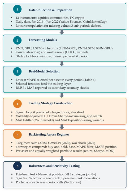
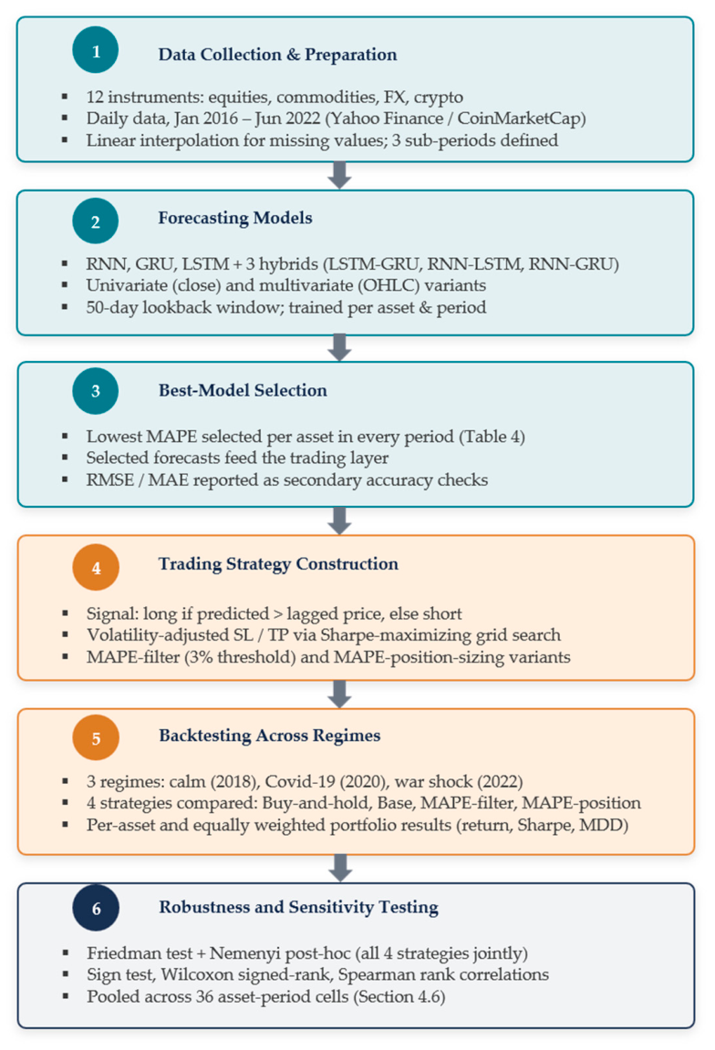
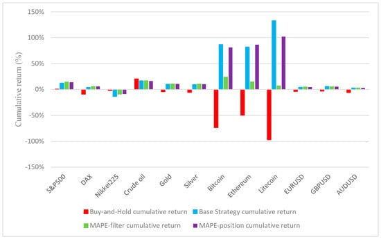
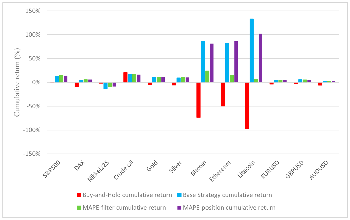
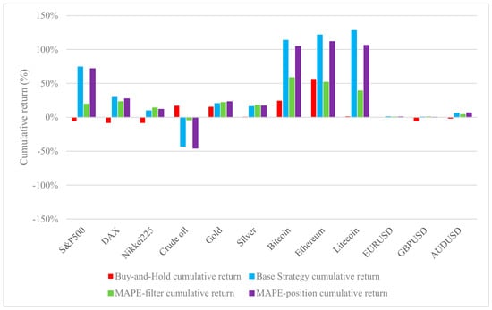
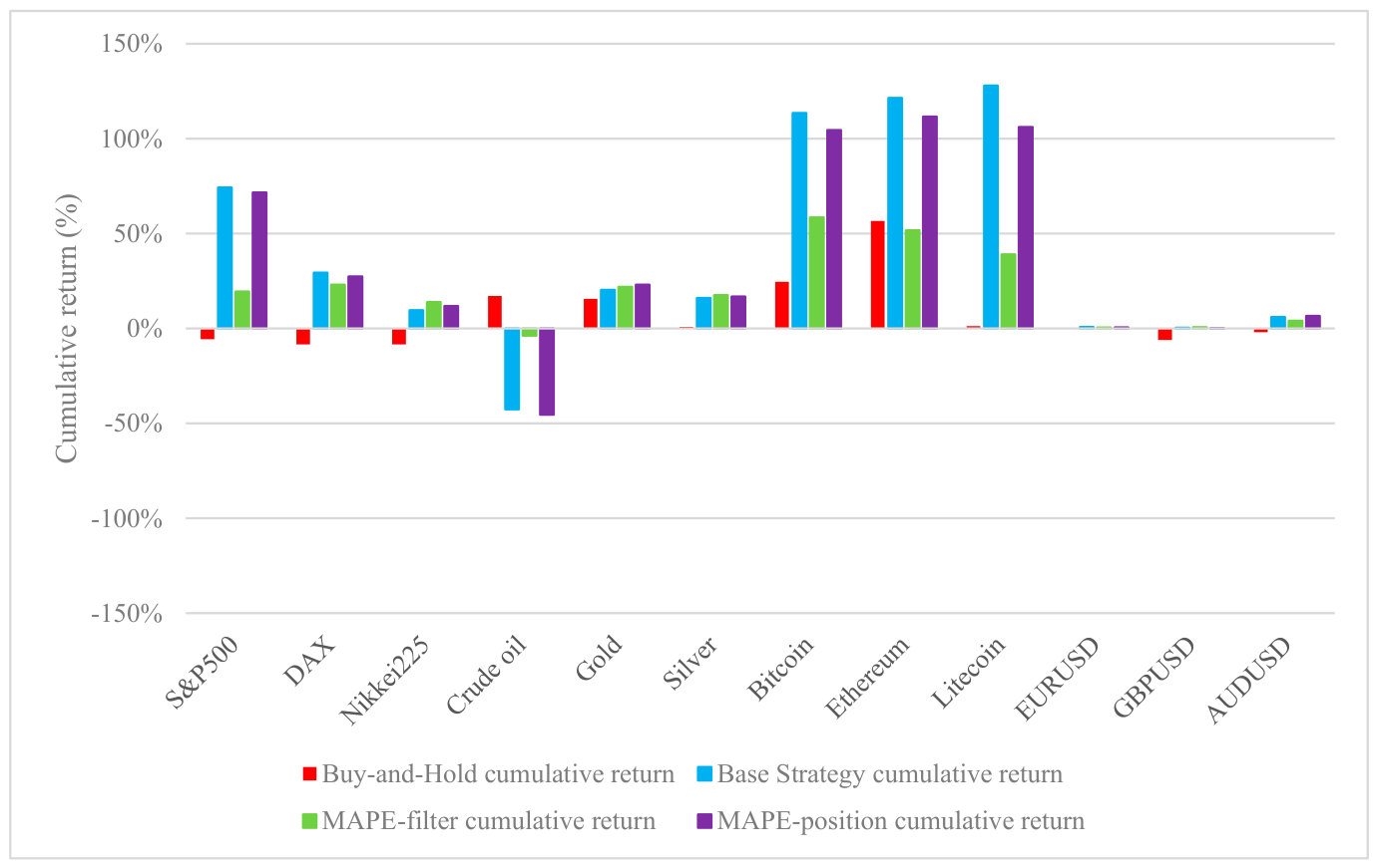
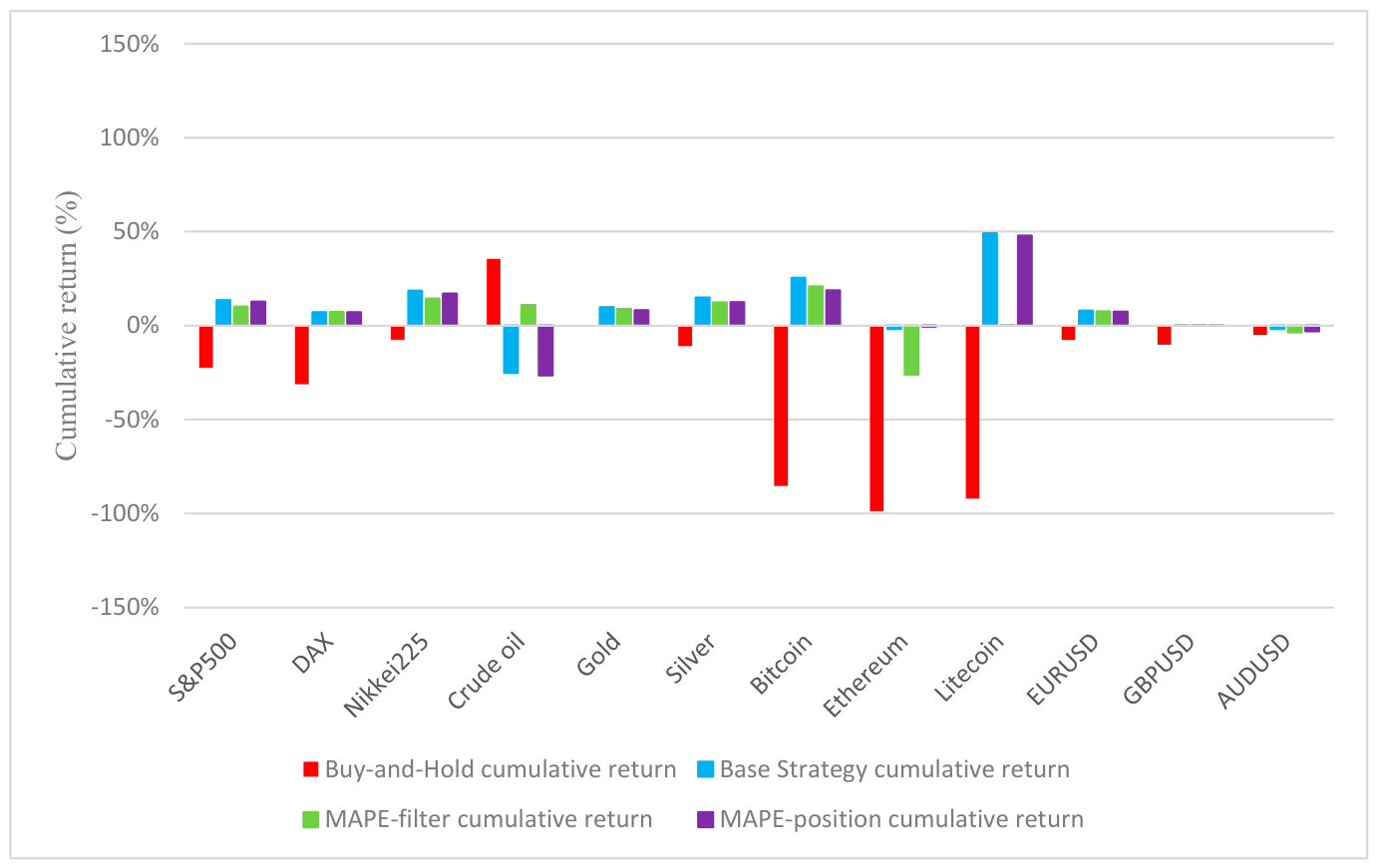
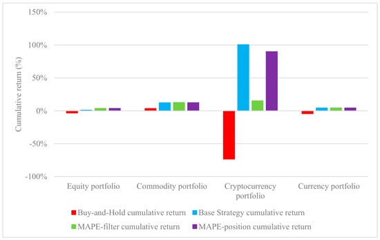
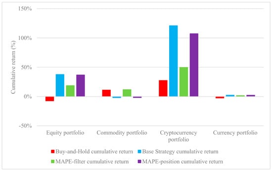
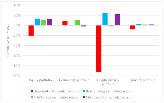
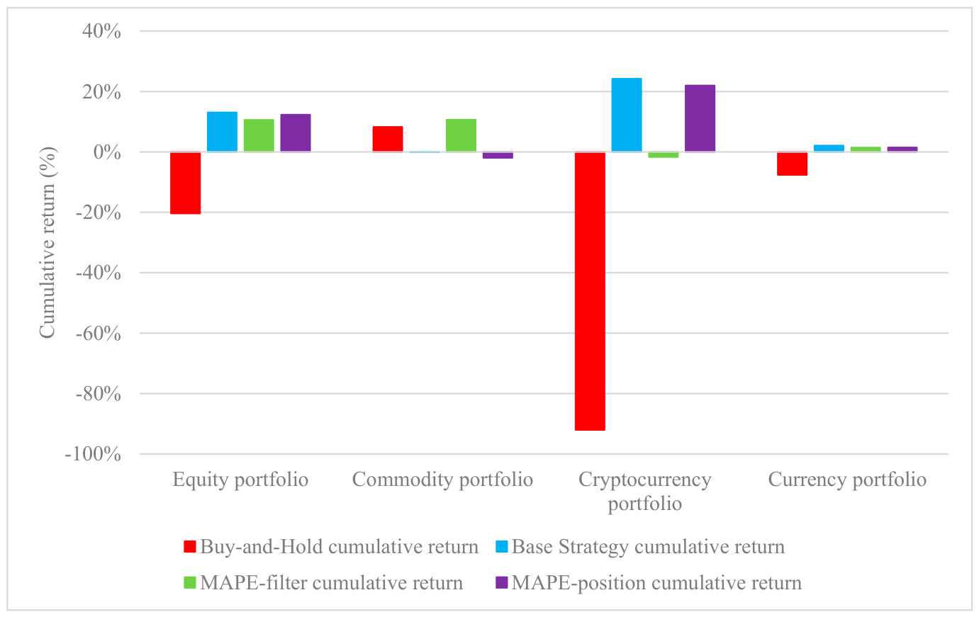
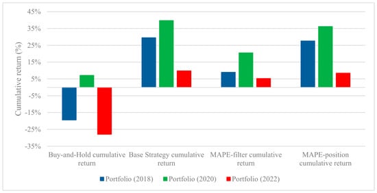
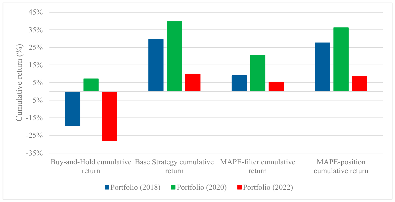

Disclaimer/Publisher’s Note: The statements, opinions and data contained in all publications are solely those of the individual author(s) and contributor(s) and not of MDPI and/or the editor(s). MDPI and/or the editor(s) disclaim responsibility for any injury to people or property resulting from any ideas, methods, instructions or products referred to in the content. |
© 2026 by the authors. Licensee MDPI, Basel, Switzerland. This article is an open access article distributed under the terms and conditions of the Creative Commons Attribution (CC BY) license.