An Empirical Model for Non-Linear Pressure Drag Across Non-Hydrostatic Flow Regimes with Trapped Lee Waves

Abstract

This study introduces a novel empirical model to estimate the total pressure drag generated by trapped lee waves (TLW) and upward-propagating internal waves in moderate-to-strong non-hydrostatic, stratified flow over a mountain ridge, as a function of flow non-linearity. The core framework is based on a two-layer atmosphere characterized by a piecewise-constant Scorer parameter, l, where a lower layer of constant $l_1$ underlies an upper layer with $l_2<l_1$. This framework incorporates key features to extend beyond idealized assumptions, providing a reliable tool for predicting non-linear flow regimes over mountainous terrain, particularly those featuring realistic vertical profiles of the Scorer parameter. To develop the empirical formulation, a micro- to mesoscale numerical model is employed to simulate realistic, non-linear flows over steep topography. The proposed empirical model yields results that compare favorably with numerical simulations across a range of moderate-to-strong non-hydrostatic regimes, including complex cases derived from observational data and realistic vertical profiles of the Scorer parameter. The model demonstrates robust performance ranging from strongly to moderately non-hydrostatic regimes (the latter corresponding to dimensionless half-widths of approximately 5), and provides accurate drag estimates for non-linearities up to a dimensionless mountain height of approximately unity. Therefore, this empirical approach serves as a valuable foundation for improving drag parameterizations in weather prediction models, offering a computationally efficient alternative to high-resolution numerical downscaling over steep terrain.

1. Introduction

The hydrostatic approximation has been adopted in many classic studies because mesoscale non-hydrostatic effects are often modest, and this assumption greatly simplifies the analysis. Consequently, most modern orographic drag parameterization schemes were developed for hydrostatic flows, with closed-form expressions for total drag derived in several foundational studies [1,2,3,4].

Since many flows over mountains are non-linear, studying the impact of non-linearity on gravity-wave drag is essential. In the hydrostatic regime, this impact is well-documented: Lilly and Klemp [5] showed how finite amplitude and asymmetry amplify drag, while Smith [6] and Durran [7] clarified the limits of linear theory and scaling laws. Furthermore, Ólafsson and Bougeault [8] and Miranda and James [9] examined drag enhancement and the transition to wave-breaking for non-dimensional mountain heights $N{h}_0/U\sim O\left(1\right)$, where drag substantially surpasses linear values.

On the other hand, as wind speed increases or static stability decreases, flow becomes increasingly non-hydrostatic. Unlike the hydrostatic regime, where all forced waves act as upward-propagating internal waves that freely transport momentum vertically into the stratosphere, non-hydrostatic scenarios render high-wavenumber components evanescent. If an evanescent layer overlies a propagating one, this upward momentum transport is halted and wave energy is reflected downward. This mechanism generates trapped lee waves (TLW)—which propagate horizontally downstream within the lower troposphere—leading to resonance and amplified drag—phenomena also possible via partial reflection under hydrostatic conditions [4,5]. Notably, non-hydrostatic drag can match or exceed its hydrostatic counterpart [10,11].

In contrast to hydrostatic flows, non-linear drag in non-hydrostatic flows has received considerably less attention. Here, “non-linear drag” refers to the flow regime where the dimensionless mountain height ${\widehat{h}}_0=N{h}_0/U$ (where N is the stability and U is the wind speed) approaches $\mathcal{O}\left(1\right)$, so that the linear assumption of small perturbations fails, causing the total drag to deviate significantly from the analytical $D\propto h_0^2$ scaling. In an analogous way, “non-hydrostatic flows” refer to the flow regime where the dimensionless width $\widehat{a}=Na/U$ is much less than 10 (e.g., $\widehat{a}\le 2$), causing vertical accelerations in the fluid to become physically significant. Among the existing literature, Peltier and Clark [12] documented amplification regimes and transitions to wave breaking, while Lott [13] analyzed how non-linear intensification of TLW TLW modes and critical-level interactions modify momentum flux. Vosper [14] demonstrated that linear theory underestimates wave amplitudes in boundary-layer (BL) inversions for short horizontal wavelengths; large amplitudes can trigger flow separation and rotors, leading to significant regime shifts in drag. Doyle and Coauthors [15], using Terrain-induced Rotor Experiment (T-REX) campaign simulations, reported how wave intensification, TLW, and rotor patterns modulate pressure drag. Moreover, Teixeira et al. [10] used a two-layer atmosphere with piecewise-constant parameters (following [16]) to show that TLW drag can equal or exceed that of vertically propagating waves, with significant implications for drag parameterizations [17]. Similarly, Teixeira et al. [11] found comparable contributions from TLW and propagating waves for lee waves trapped at an inversion capping a neutral layer. Despite these foundational studies, a comprehensive mapping of drag as a function of non-linearity in non-hydrostatic flows featuring TLW is still lacking. Recently, Argain [18] verified that non-linearity is comparably important for the drag produced by both upward-propagating waves and TLW. Therefore, further studies are essential to better understand this drag behaviour and to establish a robust basis for more accurate parameterization schemes in weather forecasting models.

For the reasons explained above, the primary motivation of this work is to develop a baseline, easily implementable empirical model that can serve as a base tool for building viable alternatives to parameterize total pressure drag under non-linear conditions. Based on the foundational two-layer configuration of Scorer [16], the proposed model is evaluated using diverse TLW cases from the literature, including aircraft observations over the Blue Ridge Mountains [19], satellite imagery of Macquarie Island [20], and wind profiler data from Hong Kong [21]. Additionally, reference profiles derived from high-resolution simulations and reanalyses [22] are used to represent upper-level evanescence regimes. The model is shown to agree well with numerical simulations for moderate-to-strong non-hydrostatic and non-linear regimes featuring TLW generation.

The article is organized as follows: Section 2 and Section 3 describe the linear and numerical models, respectively. Section 4 introduces the empirical model, its theoretical basis, and its practical implementation procedure. Section 5 provides the model validation and discussion, and finally, Section 6 offers concluding remarks.

2. Linear Model

We consider a linear model for a steady, inviscid, non-rotating, and stratified flow over a two-dimensional (2D) mountain ridge of relatively small amplitude, oriented perpendicularly to the incident flow. The spatial scale of the flow is large enough that viscous effects are negligible (i.e., a free-atmosphere flow rather than a BL flow), yet sufficiently small that the Earth’s rotation can be safely ignored (implying a large Rossby number, $Ro\gg 1$).

By linearizing the equations of motion under the Boussinesq approximation about a reference mean state and expressing the dependent variables as Fourier integrals in x, the Fourier transform of the vertical-velocity perturbation, $w_k$, is shown to satisfy the stationary form of the Taylor–Goldstein equation [3,16]:

$${\displaystyle \frac{{\partial }^2{w}_k}{\partial z^2}}+\left(l^2-k^2\right)w_k=0,\mathrm{with}l={\left({\displaystyle \frac{N^2}{U^2}}-{\displaystyle \frac{1}{U}}{\displaystyle \frac{d^{2}U}{d{z}^2}}\right)}^{1/2},$$

(1)

where l is the Scorer parameter of the atmosphere. Mathematically, the non-hydrostaticity of the flow is expressed in Equation (1) when the horizontal wavenumber k is of the same order of magnitude as the Scorer parameter l, meaning the $k^2$ term cannot be neglected compared to $l^2$. Here, k is the horizontal wavenumber in the x direction, $N^2\left(z\right)=(g/\theta )(d\theta /dz)>0$ is the Brunt–Väisälä (buoyancy) frequency of the reference state (g being the gravitational acceleration and $\theta$ the potential temperature), and $U\left(z\right)$ is the incoming wind speed perpendicular to the ridge. Consistent with the Boussinesq approximation applied above, the atmospheric fluid is essentially treated as incompressible except where density variations generate these buoyancy forces. Equation (1) describes how the amplitude of the vertical velocity perturbation for each wavenumber varies with altitude, depending on the vertical structure of the atmosphere through $l\left(z\right)$. The existence of TLWs fundamentally requires that the squared Scorer parameter, $l^2\left(z\right)$, decreases with height sufficiently for high-wavenumber components to become evanescent aloft while remaining vertically propagating below. Specifically, there must exist wavenumbers k satisfying $l_2<k<l_1$. This condition is a strict prerequisite for the formation of trapped modes within the lower tropospheric waveguide.

In this model, the atmosphere is divided into vertical layers, each with a constant Scorer parameter. Within each layer, the vertical velocity solution takes a simple mathematical form: either a combination of oscillatory functions (if the flow is propagating) or exponential functions (if it is evanescent), depending on the relationship between the horizontal wavenumber and the local Scorer parameter.

Boundary conditions are imposed to determine the arbitrary constants in each layer. At the surface ($z=0$), $w_k$ is determined by the orography ($h_k$), as the incident flow is vertically displaced by the underlying topography. At the interfaces between layers, continuity of vertical velocity and pressure (or its vertical derivative) is required to ensure smooth transitions. Finally, a radiation condition is applied at the top of the uppermost layer to ensure that waves propagate upward or decay without artificial reflection. Once the system has been solved for each wavenumber, the complex amplitude $w_k(k,z)$ is determined for any altitude.

From the linearised horizontal momentum equation, the pressure perturbation $p_k$ can be expressed in terms of the vertical velocity and its vertical derivative:

$$p_k={\displaystyle \frac{{\rho }_0}{ik}}\left(U\left(z\right){\displaystyle \frac{\partial w_k}{\partial z}}+w_k{\displaystyle \frac{\partial U}{\partial z}}\right).$$

(2)

Evaluating this expression at $z=0$ yields the amplitude of the surface pressure perturbation for each wavenumber.

The spatial distribution of the surface pressure, $p(x,z=0)$, is reconstructed via an inverse Fourier transform. Finally, the pressure drag force across the ridge, per unit length in the span-wise direction, is defined as:

$$D={\int }_{-\infty }^{+\infty }p(x,z=0){\displaystyle \frac{\partial h}{\partial x}}dx.$$

(3)

Physically, Equation (3) represents the net horizontal force exerted by the pressure perturbation integrated along the topographic slope [3]. It is important to note how this linear wave drag differs from its non-linear counterpart mathematically. Formula (2) strictly represents the linear drag. By assuming an infinitesimally small topographic amplitude, the lower boundary condition is linearized and evaluated at the flat reference level $z=0$. Since both the pressure perturbation $p(x,z=0)$ and the topographic gradient $\partial h/\partial x$ are directly proportional to the mountain height $h_0$, this linear drag scales perfectly with $h_0^2$. In contrast, non-linear drag (which dominates when ${\widehat{h}}_0\sim \mathcal{O}\left(1\right)$) dictates that the exact boundary condition must be applied at the actual physical surface $z=h\left(x\right)$. In such finite-amplitude regimes, evaluating the pressure along the actual terrain—as performed by the numerical model in Section 3—yields a total drag that deviates significantly from the $h_0^2$ scaling.

The model described above (hereafter referred to as the Drag Linear Model (DLM) is primarily used to compute the resonance modes, characterized by their wavenumber $k_{tlw}$ (or wavelength ${\lambda }_{tlw}=2\pi /k_{tlw}$), and the total linear pressure drag, $D_L$. Additionally, the linear theoretical models of Teixeira et al. [10] and Teixeira et al. [11] are employed. Developed under the same assumptions, these models are applied to idealized atmospheric configurations and allow D to be partitioned into TLW drag ($D_{tlw}$) and vertically propagating wave drag ($D_{pw}$): $D=D_{tlw}+D_{pw}$.

Finally, the orography is assumed to be a symmetric, bell-shaped ridge:

$$h\left(x\right)={\displaystyle \frac{h_0}{1+{(x/a)}^2}}⟹h_k\left(k\right)={\displaystyle \frac{h_{0}a}{2}}{e}^{-a\left|k\right|},$$

(4)

where $h_0$ is the maximum height and a is the half-width.

3. Numerical Model

Unlike the linear model presented in Section 2, which is formulated in Cartesian coordinates, this study employs the FLEX model. The name “FLEX” stands for “flexible,” highlighting its ability to simulate a wide range of flow types—from BL flows to outer free-atmosphere flows—regardless of the degree of non-linearity or hydrostaticity. As a 2D micro-to-mesoscale numerical model formulated in orthogonal curvilinear coordinates, it has been previously used to investigate resonant mountain waves [10,11,23,24,25]. The use of such a terrain-following coordinate system is essential for accurately studying the effects of increasing the mountain height ($h_0$) into the non-linear regime, as it prevents grid distortion and the subsequent penalization of numerical accuracy that typically occurs over steep orography.

The vertical spacing is $\Delta z=25$ m. The horizontal resolution $\Delta x$ is the minimum of ${\lambda }_{tlw,min}/40$ and $a/5$, ensuring at least 40 points per minimum TLW wavelength and 5 points per mountain half-width. It should be noted that $\Delta x$ and $\Delta z$ represent the constant grid spacings within the uniform computational domain, which are subsequently mapped onto the physical space via the orthogonal curvilinear transformation. The computational domain extends vertically to a height of six hydrostatic vertical wavelengths (${\lambda }_{z0}=2\pi /l_1$). Horizontally, it spans $7a$ upstream and $15{\lambda }_{tlw,max}$ downstream. Here, ${\lambda }_{tlw,min}$ and ${\lambda }_{tlw,max}$ denote the shortest and longest wavelengths, respectively, for configurations where multiple TLW modes coexist; in single-mode cases, both default to the unique wavelength, ${\lambda }_{tlw}$. The integration time step is set to $\Delta t=1$ s.

A $2.5{\lambda }_{z0}$ top sponge layer is applied, while a radiation condition and lateral sponges are used at the boundaries. FLEX is calibrated using $D_L$ values from the DLM, as the total drag D is sensitive to boundary-absorbing sponges. Accurate $D_L$ calculation is vital, as it is used to normalize D in the empirical model.

4. Empirical Model

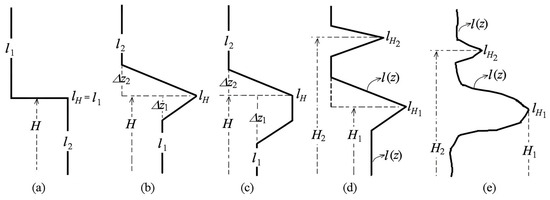
Figure 1 illustrates the various atmospheric configurations considered for the development of the empirical model. Figure 1a depicts the two-layer Scorer atmosphere which, as previously noted, forms the basis of this drag empirical model (DEM). In this baseline configuration, the DLM and FLEX models employ a uniform background wind of $U=10$ m s⁻¹ (so the curvature term vanishes). Static stability is prescribed as $N_1=0.02$ s⁻¹ in the lower layer and $N_2=0.004$ s⁻¹ in the upper layer, resulting in $N_2/N_1=0.2$ and $l_2/l_1=0.2$.

Figure 1. Vertical profiles of the Scorer parameter, $l\left(z\right)$, representing the diverse atmospheric configurations used to develop the DEM. In all panels, the vertical axis represents altitude (z) and the horizontal axis denotes the Scorer parameter (l). (a) The classical two-layer Scorer atmosphere, featuring a constant lower layer ($l_1$) and upper layer ($l_2$) separated by an interface at height H (where $l_H=l_1$). (b) An idealized profile with a continuous transition to a maximum $l_H$ over a vertical distance $\Delta z_1$, followed by a decay over $\Delta z_2$. (c) An idealized profile featuring a maximum $l_H$ at a sharp discontinuity (plateau edge). (d,e) Idealized and realistic (arbitrary) profiles, respectively, featuring multiple discrete wave-trapping maxima ($l_{H_1}$, $l_{H_2}$) at specific altitudes ($H_1$, $H_2$).

For the two-layer Scorer profile (Figure 1a), the dimensionless mountain height and half-width are determined as ${\widehat{h}}_0=N_1{h}_0/U=l_1{h}_0$ and $\widehat{a}=N_{1}a/U=l_{1}a$. For more complex profiles, such as those illustrated in Figure 1b–e, ${\widehat{h}}_0$ and $\widehat{a}$ are defined using the maximum value of $l\left(z\right)$, closest to the surface, that produces TLW. For instance, in the case of the profile in Figure 1c, ${\widehat{h}}_0=l_H{h}_0$ and $\widehat{a}=l_{H}a$, while for Figure 1d, ${\widehat{h}}_0=l_{H_1}{h}_0$ and $\widehat{a}=l_{H_1}a$.

In all cases, a bell-shaped mountain (4) is used to control a and $h_0$ variations. Non-linearity is modulated via $h_0$, from the linear regime (${\widehat{h}}_{0,L}=0.02$) up to ${\widehat{h}}_0\approx 1$ (e.g., $h_0$ ranging from approximately 10 m to 500 m, for typical $l_1$ values). Larger ${\widehat{h}}_0$ values are omitted because, as shown by Argain [18], TLW effects on drag variability—the dominant driver in this flow regime—become secondary for ${\widehat{h}}_0>1$. Consistent with that study, no wave breaking was observed in our simulations. Indeed, when atmospheric conditions strongly favor wave trapping in the lower layers, vertical energy propagation is severely restricted, effectively suppressing classic mid-tropospheric wave breaking even at higher non-linearities (e.g., Doyle and Reynolds [26]). Therefore, the associated drag enhancement typical of breaking waves is absent.

4.1. DEM for a Two-Layer Scorer Atmosphere

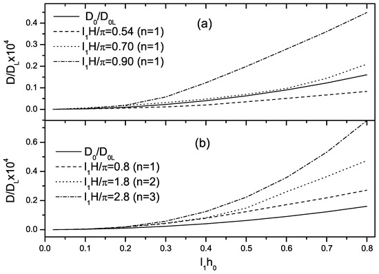
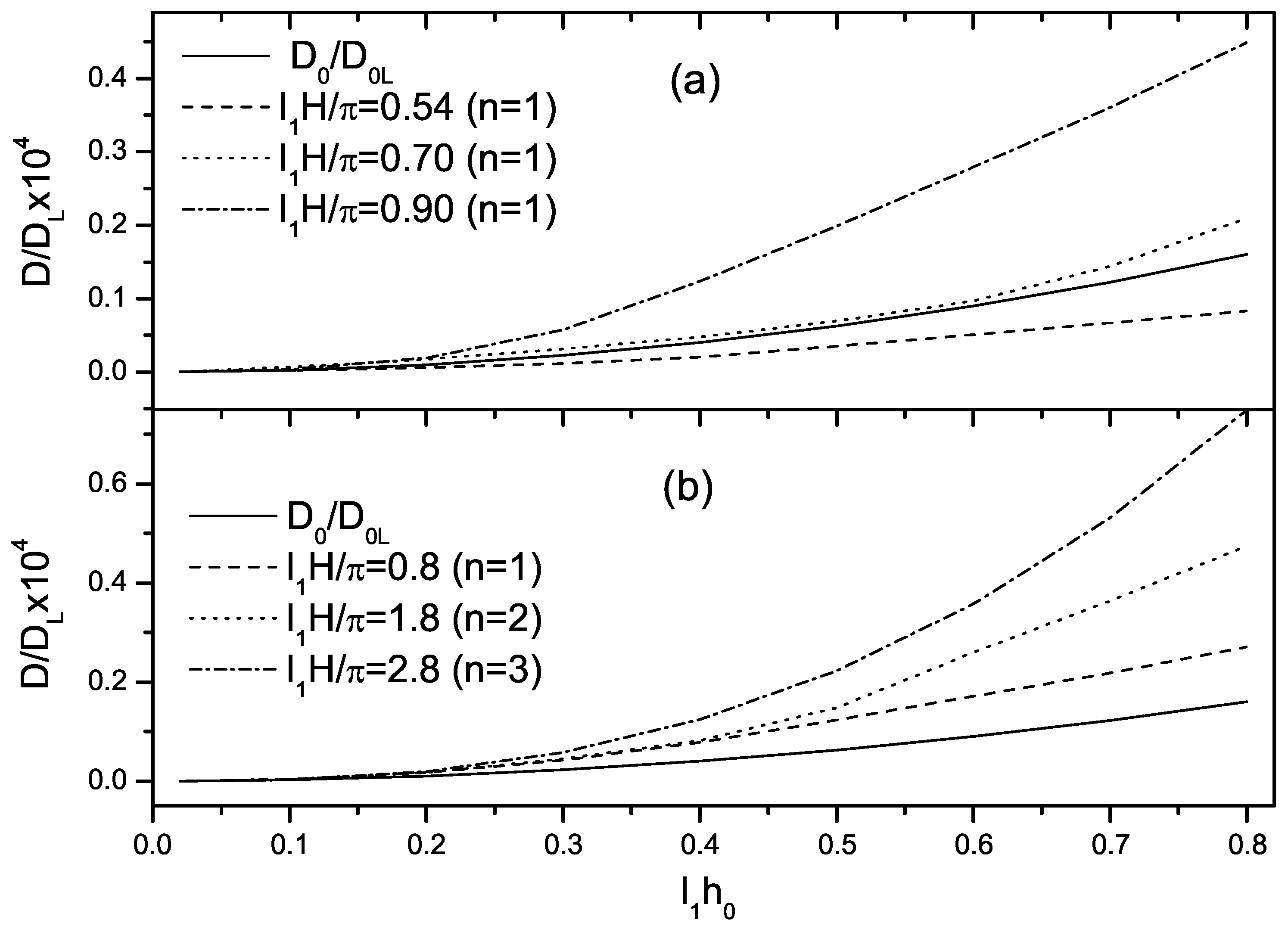
Figure 2 shows the normalised linear drag $D_L/D_{L,0}$ and its components ($D_{L,tlw}$ and $D_{L,pw}$) as a function of $\widehat{H}\in [0.5, 3.0]$, calculated following Teixeira et al. [10] for a Scorer atmosphere (Figure 1a). Results are presented for moderate ($\widehat{a}=5, a=2500$ m; Figure 2a) and strong ($\widehat{a}=2, a=1000$ m; Figure 2b) non-hydrostatic effects, both in the linear regime (${\widehat{h}}_{0,L}=0.02$). Here, $D_{L,0}=0.25\pi {\rho }_0{l}_1{\left(h_{0,L}U\right)}^2$ is the linear hydrostatic reference.

Figure 2. Normalized total linear drag $D_L/D_{L,0}$ (solid lines) and its trapped ($D_{L,tlw}/D_{L,0}$, dotted lines) and propagating ($D_{L,pw}/D_{L,0}$, dashed lines) components vs. dimensionless duct depth $\widehat{H}$, from the model of Teixeira et al. [10]. (a) $\widehat{a}=5$ (moderate non-hydrostatic effect, $a=2500$ m). (b) $\widehat{a}=2$ (strong non-hydrostatic effect, $a=1000$ m). Here, $D_{L,0}=0.25\pi {\rho }_0{l}_1{\left(h_{0,L}U\right)}^2$ is the linear hydrostatic reference (${\widehat{h}}_{0,L}=0.02$ is the linear dimensionless mountain height).

Notably, in non-hydrostatic regimes (Figure 2b), $D_{L,tlw}$ can equal or exceed $D_{L,pw}$, representing a substantial fraction of the total drag. In Figure 2a (moderately non-hydrostatic), $D_{L,tlw}$ remains below $D_{L,pw}$ but still accounts for $\approx 50\%$ of the total drag. This contrasts with classical hydrostatic cases where the TLW contribution is negligible (see Figure 17a in [10]). Generally, flows where $D_{L,tlw}\sim D_L$ exhibit moderate-to-strong non-hydrostaticity ($\widehat{a}\approx 1$–5), which is the focus of this study. A key insight for the DEM, derived from Figure 2a,b, is the similarity in the functional form of drag across different trapped modes. Specifically, while the maximum intensity of the normalized drag ($D_L/D_{L,0}$) at the resonance peaks gradually decreases as the mode number increases (i.e., the peak amplitude for $n=1$ is greater than for $n=2$, and so forth), the underlying structural shape of the resonance curves remains remarkably consistent for successive modes. This repeated geometric profile justifies modelling the drag using a single unified empirical base function, which can then be accurately adjusted for each individual mode by applying a mode-dependent amplitude scaling factor depending on n. This insight inspired the formulation of a generic drag function, $D\left(\widehat{H}\right)$, calibrated for the first mode ($n=1$) within $\widehat{H}\in [0.5,1.5]$, which is then scaled to reconstruct the behavior of higher-order modes ($n>1$).

Figure 3a illustrates $D/D_L({\widehat{h}}_0)$ profiles for $\widehat{H}=0.54$, $0.7$, and $0.9$ (within the $n=1$ range, $\widehat{H}\in [0.5,1.5]$). Figure 3b presents analogous profiles for different modes: $\widehat{H}=0.8$ ($n=1$), $\widehat{H}=1.8$ ($n=2$), and $\widehat{H}=2.8$ ($n=3$). Furthermore, for comparison, both plots include a linear extrapolation of the hydrostatic single-layer total drag, $D_L=0.25\pi {\rho }_0{l}_1{\left(h_{0}U\right)}^2$, normalized by the linear value $D_{L,0}$.

Figure 3. Numerical $D/D_L$ profiles for various $\widehat{H}$, obtained with the FLEX model. (a) $D/D_L\left({\widehat{h}}_0\right)$ ($n=1$) for $\widehat{H}=0.54$, $0.7$, and $0.9$. (b) $\widehat{H}=0.8$ ($n=1$), $\widehat{H}=1.8$ ($n=2$), and $\widehat{H}=2.8$ ($n=3$). $D_0/D_{L,0}$ is the linear extrapolation of the hydrostatic single-layer total drag, $D_L=0.25\pi {\rho }_0{l}_1{\left(h_{0}U\right)}^2$, normalized by the linear value $D_{L,0}=0.25\pi {\rho }_0{l}_1{(h_{0,L}U)}^2$.

Consistent with Argain [18], the $n=1$ profiles (Figure 3a) exhibit a quadratic behaviour ($D/D_L\propto {\widehat{h}}_0^2$), suggesting that the linear scaling is preserved and can be fitted by an expression of the form $\mathsf{\Phi }(\tilde{H}){\tilde{h}}_0^2+1$. In Figure 3b, the $n=1$ and $n=2$ profiles coincide up to ${\widehat{h}}_0\approx 0.5$ before $n=2$ diverges toward higher drag. A similar trend occurs for $n=3$, with divergence starting earlier at ${\widehat{h}}_0\approx 0.3$. These results indicate that both the quadratic exponent and $\mathsf{\Phi }$ must be adjusted (increased) as the mode number n increases. In this formulation, this is achieved by multiplying $\mathsf{\Phi }(\tilde{H})$ by a function of the form ${\left[{\tilde{h}}_0^{\beta }\mathsf{\Psi }\left(\tilde{H}\right)\right]}^{n-1}$.

Based on a detailed analysis of all numerical profiles, the following expression is proposed to estimate D for the two-layer Scorer model (using the $l\left(z\right)$ profile shown in Figure 1a), for arbitrary values of n and $\widehat{H}$:

$${\displaystyle \frac{D}{D_L}}\left({\tilde{h}}_0\right)=\mathsf{\Phi }\left(\tilde{H}\right){\tilde{h}}_0^2{\left[{\tilde{h}}_0^{1/5}\mathsf{\Psi }\left(\tilde{H}\right)\right]}^{n-1}+1,$$

(5)

where ${\tilde{h}}_0={\widehat{h}}_0/{\widehat{h}}_{0,1}-1$ and $\tilde{H}=\widehat{H}/0.5-1$. In this formulation, ${\widehat{h}}_{0,1}$ represents the minimum dimensionless mountain height considered in the numerical simulations. (It should be noted that the fractional exponent 1/5 is empirically derived to optimally capture the drag amplification). Furthermore, $\widehat{H}$ is adjusted such that $\widehat{H}=\widehat{H}+0.5$ if $\widehat{H}<0.5$, and $\widehat{H}=\widehat{H}-\mathrm{nint}(\widehat{H})+1$, where $\mathrm{nint}$ denotes the nearest integer function. The parameters $D_L$ and n are determined using the DLM framework.

The functions $\mathsf{\Phi }(\tilde{H})$ and $\mathsf{\Psi }(\tilde{H})$ are defined by the following expressions:

$$\mathsf{\Phi }\left(\tilde{H}\right)=a_{1}exp[+a_2{\tilde{H}}^{a_3}]+a_4{\tilde{H}}^{a_5}+a_6\mathrm{for}\widehat{H}\le 1.032$$

(6)

$$\mathsf{\Phi }\left(\tilde{H}\right)=b_{1}exp[-b_2{\tilde{H}}^{b_3}]+b_4{\tilde{H}}^{b_5}+b_6\mathrm{for}\widehat{H}>1.032$$

(7)

$$\mathsf{\Psi }\left(\tilde{H}\right)=c_1+{\displaystyle \frac{c_2-c_1}{1+exp\left[c_3(\tilde{H}-c_4)\right]}}\mathrm{for}\widehat{H}\le 0.825$$

(8)

$$\mathsf{\Psi }\left(\tilde{H}\right)=d_2{\tilde{H}}^2+d_1\tilde{H}+d_0\mathrm{for}\widehat{H}>0.825.$$

(9)

To determine the empirical coefficients for the functions $\mathsf{\Phi }(\tilde{H})$ and $\mathsf{\Psi }(\tilde{H})$, optimization methods based on the least-squares criterion were applied. Specifically, the polynomial components were fitted using standard linear regression (via MATLAB R2025b’s polyfit routine), while the non-linear components were obtained by minimizing a non-linear sum-of-squared-errors cost function using the fminsearch routine. For the non-linear components, the fit was achieved by minimizing a non-linear sum-of-squared-errors cost function. It is important to emphasize that the mathematical form chosen for these non-linear components—a logistic (sigmoid) function—was deliberately selected to guarantee a stable asymptotic behavior. This formulation ensures that the drag corrections remain bounded, preventing numerical divergences or unrealistic drag amplification if the DEM is extrapolated to flow configurations slightly outside the strictly tested parameter domain.

The sets of constants $a_i, b_i, c_i,$ and $d_i$, derived from fitting, are as:

(a)

$a_1=-0.0007272$, $a_2=7.0221$, $a_3=1.0645$, $a_4=4.61$, $a_5=2.3724$, and $a_6=0.56966$;

(b)

$b_1=2.8863$, $b_2=0.031476$, $b_3=19$, $b_4=0.056042$, $b_5=-1.1833$, and $b_6=2.1822$;

(c)

$c_1=0.642$, $c_2=1.0026$, $c_3=20.7235$, and $c_4=0.29845$;

(d)

$d_2=0.76594$, $d_1=-2.31083$ and $d_0=1.748$.

These functions are specifically designed to capture the regime transitions and modal dependence inherent in moderate-to-strong non-hydrostatic flows. By distinguishing between different ranges of the dimensionless duct depth $\widehat{H}$, the model accounts for the shifting dominance of TLW modes. Furthermore, the high precision of the reported constants is essential for the numerical reproducibility of the DEM, ensuring consistent drag estimations across the diverse atmospheric configurations explored in this study.

Modes are limited to $n=3$, as higher-order configurations are rare in nature and increase model complexity without proportional practical gains. Furthermore, numerical simulations show that achieving a quasi-stationary state for D becomes increasingly difficult as n increases, requiring greater computational effort to ensure convergence.

4.2. DEM for an Arbitrary Atmosphere

A key feature of the DEM is the normalization by $D_L$, which ensures $D/D_L=1$ in the linear limit and standardizes results across distinct $l\left(z\right)$ structures. As demonstrated below, simulations using various idealized configurations (Figure 1a–d) with identical $\widehat{H}$ show that $D/D_L({\widehat{h}}_0)$ profiles remain remarkably similar, often nearly coincident.

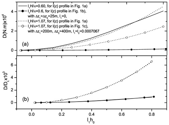
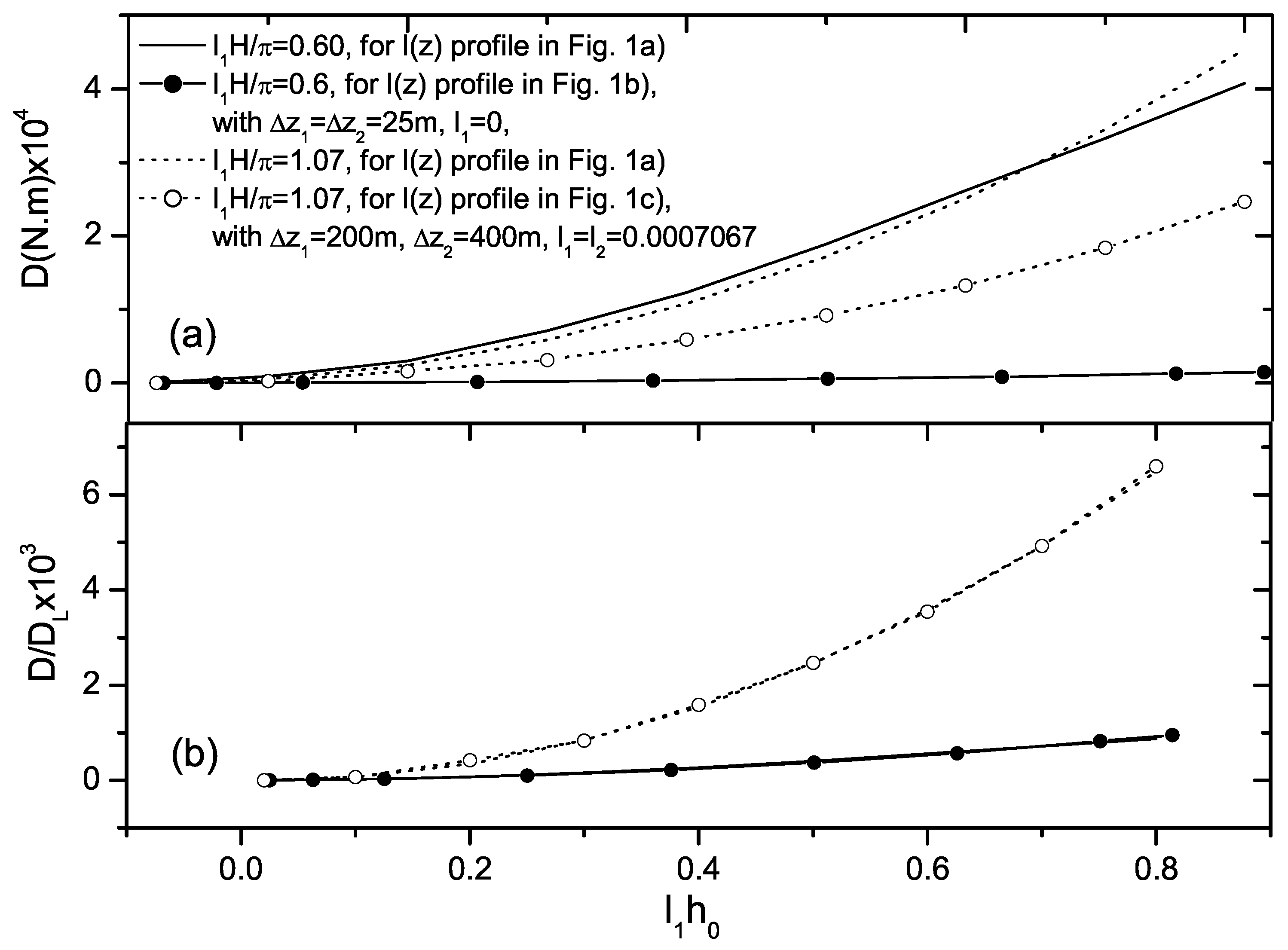
Figure 4a contrasts the $D({\widehat{h}}_0)$ profiles (i.e., not normalized by $D_L$) for $\widehat{H}=0.6$ and $\widehat{H}=1.07$ to illustrate how the geometry of the $l\left(z\right)$ profile influences drag. For $\widehat{H}=0.6$, the solid line with solid circles represents an extreme case where waves are trapped by a thin inversion capping a neutral layer ($l\left(z\right)$ profile in Figure 1b with $l_1=0$ m⁻¹), a flow regime investigated by Teixeira et al. [11]. This configuration features an inversion at $H=500$ m ($l_H=1.25\times {10}^{-3}$ m⁻¹, $\Delta z_1=\Delta z_2=25$ m) with $l_2=1\times {10}^{-3}$ m⁻¹ aloft. The solid line corresponds to the $l\left(z\right)$ profile in Figure 1a with the same parameters but with $\Delta z_1=\Delta z_2=0$.

Figure 4. (a) Non-normalized $D({\widehat{h}}_0)$ profiles and (b) normalized $D/D_L({\widehat{h}}_0)$ profiles for two different cases of $l_{1}H/\pi$: $0.6$ and $1.07$. In (a), solid lines denote the $l\left(z\right)$ profile from Figure 1a for $l_{1}H/\pi =0.6$, and solid lines with solid circles denote the $l\left(z\right)$ profile from Figure 1b for the same ratio. Similarly, dotted lines denote the $l\left(z\right)$ profile from Figure 1a for $l_{1}H/\pi =1.07$, and dotted lines with open circles denote the $l\left(z\right)$ profile from Figure 1c for the same ratio. The same line styles and symbols apply to subfigure (b).

For $\widehat{H}=1.07$, the dotted line with open symbols corresponds to an $l\left(z\right)$ profile of the type shown in Figure 1c with the following parameters: $H=1000$ m, $l_H=2.8\times {10}^{-3}$ m⁻¹, $l_1=1.4\times {10}^{-3}$ m⁻¹, $l_2=2.8\times {10}^{-4}$ m⁻¹, $\Delta z_1=200$ m, and $\Delta z_2=400$ m. The dotted line with open circles represents the baseline Scorer profile in Figure 1a for $\widehat{H}=1.07$ (same parameters but with $\Delta z_1=\Delta z_2=0$). A comparison of these $D({\widehat{h}}_0)$ profiles reveals that, consistent with the previous case, they differ considerably.

Using the same symbology, Figure 4b shows the same profiles as Figure 4a, but normalized by $D_L$. The high degree of coincidence observed for both $\widehat{H}=0.6$ and $1.07$ confirms that $D_L$-normalization enables the two-layer Scorer model to serve as a universal baseline for the DEM across distinct $l\left(z\right)$ structures with identical $\widehat{H}$.

Notably, the non-normalized Scorer (solid line) and thin-inversion (dotted line) profiles diverge significantly despite sharing the same $\widehat{H}$.

Additional tests with $l\left(z\right)$ profiles featuring multiple $l_H$ maxima, such as that in Figure 1d, confirm that $D_L$-normalization is equally effective for these configurations. In such cases, the normalised total surface drag $D({\tilde{h}}_0)$ is effectively the sum of the contributions from each maximum. Thus, following Equation (5), the total drag is:

$${\displaystyle \frac{D}{D_L}}\left({\tilde{h}}_0\right)={\displaystyle \frac{1}{D_L}}{\displaystyle \sum _{i=1}^m}{D}_i({\tilde{H}}_i,{\tilde{h}}_0,n_i),$$

(10)

where m is the number of contributing maxima, $D_L$ is the total linear drag computed by the DLM for the full $l\left(z\right)$ profile, while $n_i$ and $D_i$ denote the number of modes and the drag contribution associated with each ${\tilde{H}}_i$, respectively. It should be noted that using the DLM is crucial for determining, by a process of elimination, which maxima effectively generate TLW.

Equation (10) defines the final formulation DEM, which is, in principle, applicable to any $l\left(z\right)$ profile.

4.3. Final Remarks on the DEM Formulation

Although the DEM intentionally smooths the abrupt drag transitions associated with mode shifts, this simplification is robustly justified. Firstly, the regions of abrupt transition are parametrically narrow. For instance, in the non-hydrostatic linear reference regime (Figure 3b), the transition from $n=1$ to $n=2$ occurs over a small interval of $\Delta \widehat{H}\approx 0.2$ (between $\widehat{H}\approx 1.4$ and $1.6$), and a similar width is observed for the $n=2$ to $n=3$ shift (between $\widehat{H}\approx 2.4$ and $2.6$). Consequently, the statistical error introduced by this smoothing over a broad climatological distribution of atmospheric states is minimal. Secondly, and more importantly from a physical standpoint, the sharp resonant discontinuities predicted by idealized piecewise-constant theory are rarely realized in the actual atmosphere. Natural variability in atmospheric profiles, transient flow effects, and three-dimensional dispersion inherently “smear” these resonant peaks. Therefore, the continuous functions of the DEM arguably provide a more realistic representation of bulk atmospheric drag than a strictly discontinuous formulation.

For shallow lower layers ($\widehat{H}<0.5$), the flow exhibits one of two distinct states: in the extremely shallow, fully sub-critical evanescent regime (e.g., $\widehat{H}\lesssim 0.4$), the atmosphere lacks the physical waveguide thickness required to sustain efficient wave trapping, rendering TLW effects negligible; conversely, the narrow band approaching the critical threshold ($0.4<\widehat{H}<0.5$) represents the resonant onset phase, where the waveguide becomes just thick enough to trigger the fundamental mode ($n=1$), causing a sharp, highly non-linear spike in drag over a narrow interval ($\Delta \widehat{H}\approx 0.2$, between $\approx 0.4$ and $0.55$). As previously discussed, the DEM intentionally smooths these abrupt mode-shift transitions to prevent unphysical hypersensitivity to small variations in atmospheric profiles and to ensure the parameterization remains bounded and predictable. Therefore, the $+0.5$ shift effectively maps this entire shallow domain—encompassing both the near-zero drag region and the narrow resonant onset—directly into the fundamental pre-resonant interval $\widehat{H}\in [0.5,1.0]$. This transformation allows the model to safely bypass abrupt mode-switching singularities. Consequently, the DEM successfully yields physically realistic drag predictions that accurately reflect the diminishing wave activity as $\widehat{H}\to 0$.

4.4. Practical Implementation Procedure of the DEM

To facilitate the practical application of the proposed model, the following clear and concise workflow (visually summarized in the flowchart of Figure 5) is recommended for its implementation:

Figure 5. Flowchart illustrating the sequential practical implementation procedure of the Drag Empirical Model (DEM).

1.

DLM Profile representation: Use the DLM to represent the vertical profile of the Scorer parameter, $l^2\left(z\right)$ (defined in Equation (1)), through a discretization into constant-value layers. This step establishes the theoretical basis for identifying wave modes.

2.

Filtering and Mode Selection: Based on the identified maxima of $l^2\left(z\right)$ in the profile, apply an exclusion criterion to determine which layers effectively support TLW. Identify only the maxima that generate genuine modes (by solving the layer-wise Taylor–Goldstein Equation (1)), thereby defining the number of interfaces, their locations (${\widehat{H}}_i$), and the respective horizontal wavenumbers ($k_n$) and eigenvalues (${\lambda }_n$).

3.

Numerical Model Calibration and Validation: Before the final DEM application, use the numerical model (FLEX) to compute the total drag (D) under reference conditions. We recommend that this calibration be primarily performed using the linear case (i.e., calculating $D_L$ according to Equation (3)), as this is typically the only robust reference value universally available. However, if estimated drag values for non-linear situations are available—derived from local observational data or site-specific campaigns—these should be prioritized for the calibration process, as they provide a more realistic basis for non-linear regimes. During this step, adjust the sponge layer characteristics (including the vertical and lateral damping coefficients and the respective layer thicknesses) and the domain dimensions (including grid resolution, horizontal and vertical domain extent) to ensure the computed drag is physically consistent and free from spurious reflections.

4.

Empirical Model (DEM) Application: With the validated modes and the determined drag D, apply the final DEM formulation (using Equation (5) for configurations with a single wave-trapping maximum, or Equation (10) for complex profiles with multiple maxima). This model allows for a robust estimation of non-linear pressure drag, integrating the contribution of the identified modes while avoiding the need for computationally expensive numerical integrations.

5. Model Validation and Discussion

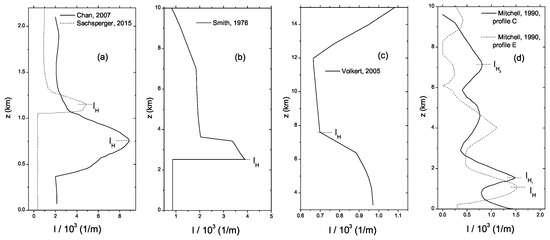
To establish a real-world benchmark for validation, atmospheric profiles derived from observational TLW field campaigns are utilized to compare the $D/D_L({\widehat{h}}_0)$ results computed by the FLEX model against those predicted by the DEM. To facilitate ${\widehat{h}}_0$ variation, a bell-shaped mountain (4) replaces actual orography. Profiles and DLM parameters (Figure 6) generally exhibit moderate non-hydrostatic effects, except for the strongly non-hydrostatic case in Volkert and collaborators [22]. All data were digitized from the original publications.

Figure 6. Observational profiles used to test the present empirical model, DEM. (a) Sachsperger et al. [27] (dotted line), Chan [21] (solid line). (b) Smith [19]. (c) Volkert and collaborators [22]. (d) Mitchell et al. [20], profile C—solid line and profile E—dotted line.

Sachsperger et al. [27] analyzed lee waves trapped at a BL inversion. Applying the DLM to the $l\left(z\right)$ profile reveals a single $l_H$ maximum and one mode ($m=1, n=1$) with: ${\lambda }_{tlw}=4974$ m, $l_H=4.87\times {10}^{-3}$ m⁻¹, $H=1153$ m, $\widehat{H}=1.79$, $a=1000$ m, and $\widehat{a}=4.9$ (moderate non-hydrostaticity).

Chan [21] studied stationary lee waves over Hong Kong ($\lambda \approx 2.8$ km). While the author suggested a single mode, the DLM identifies two TLW modes ($m=1, n=2$) from a single $l_H$ maximum. Parameters include ${\lambda }_{tlw1}=2740$ m, ${\lambda }_{tlw2}=942$ m, $l_H=8.9\times {10}^{-3}$ m⁻¹, $H=750$ m, $\widehat{H}=2.12$, $a=450$ m, and $\widehat{a}=4$ (moderate non-hydrostaticity).

Smith [19] reported aircraft observations of lee waves over the Blue Ridge Mountains, where vertical trapping was driven by an $l\left(z\right)$ profile decaying aloft. Similar to Sachsperger et al. [27], this case features $m=1, n=1$. Parameters: ${\lambda }_{tlw}=7450$ m, $l_H=3.9\times {10}^{-3}$ m⁻¹, $H=2520$ m, $\widehat{H}=3.13$, $a=1000$ m, $\widehat{a}=3.9$ (moderate non-hydrostaticity).

Volkert and collaborators [22] presented a phase diagram distinguishing between trapped lee waves (TLWs) and vertically propagating mountain waves based on the $l\left(z\right)$ profile. Unlike the direct observational data from other authors discussed herein, the profiles in Volkert and collaborators [22] represent reference cases derived from high-resolution numerical simulations performed with the Meso-Scale Non-Hydrostatic (MESO-NH) model and meteorological reanalyses. For the specific reference case selected from Volkert and collaborators [22], similarly to the case of Chan [21], the DLM reveals two TLW modes associated with a single $l_H$ maximum ($m=1$, $n=2$). The corresponding flow and terrain parameters are $l_H=7\times {10}^{-4}$ m⁻¹, ${\lambda }_{\mathrm{tlw},1}=14615$ m, ${\lambda }_{\mathrm{tlw},2}=8820$ m, $H=7609$ m, $\widehat{H}=1.69$, $a=2000$ m, and $\widehat{a}=1.4$ (strong non-hydrostaticity).

Finally, Mitchell et al. [20] presented satellite observations of TLW over Macquarie Island. We utilize profiles C and E; both contain local $l\left(z\right)$ maxima that do not produce waves ($7.7\times {10}^{-4}$ m⁻¹ at 4600 m for C, and $1.1\times {10}^{-3}$ m⁻¹ at 4000 m for E). Profile E reveals one mode ($m=1, n=1$) with: $l_H=1.52\times {10}^{-3}$ m⁻¹, ${\lambda }_{tlw}=8650$ m, $H=1095$ m, $\widehat{H}=0.53$, $a=1000$ m, $\widehat{a}=1.5$ (strong non-hydrostatic effects). Profile C exhibits two maxima and two modes ($m=2, n_1=1, n_2=1$) with: $l_{H_1}=1.47\times {10}^{-3}$ m⁻¹, ${\lambda }_{tlw,1}=8920$ m, $H_1=1536$ m, ${\widehat{H}}_1=0.72$, $l_{H_2}=7.93\times {10}^{-4}$ m⁻¹, ${\lambda }_{tlw,2}=13250$ m, $H_2=7104$ m, ${\widehat{H}}_2=1.79$, $a=2000$ m, $\widehat{a}=2.94$ (moderate-to-strong non-hydrostaticity).

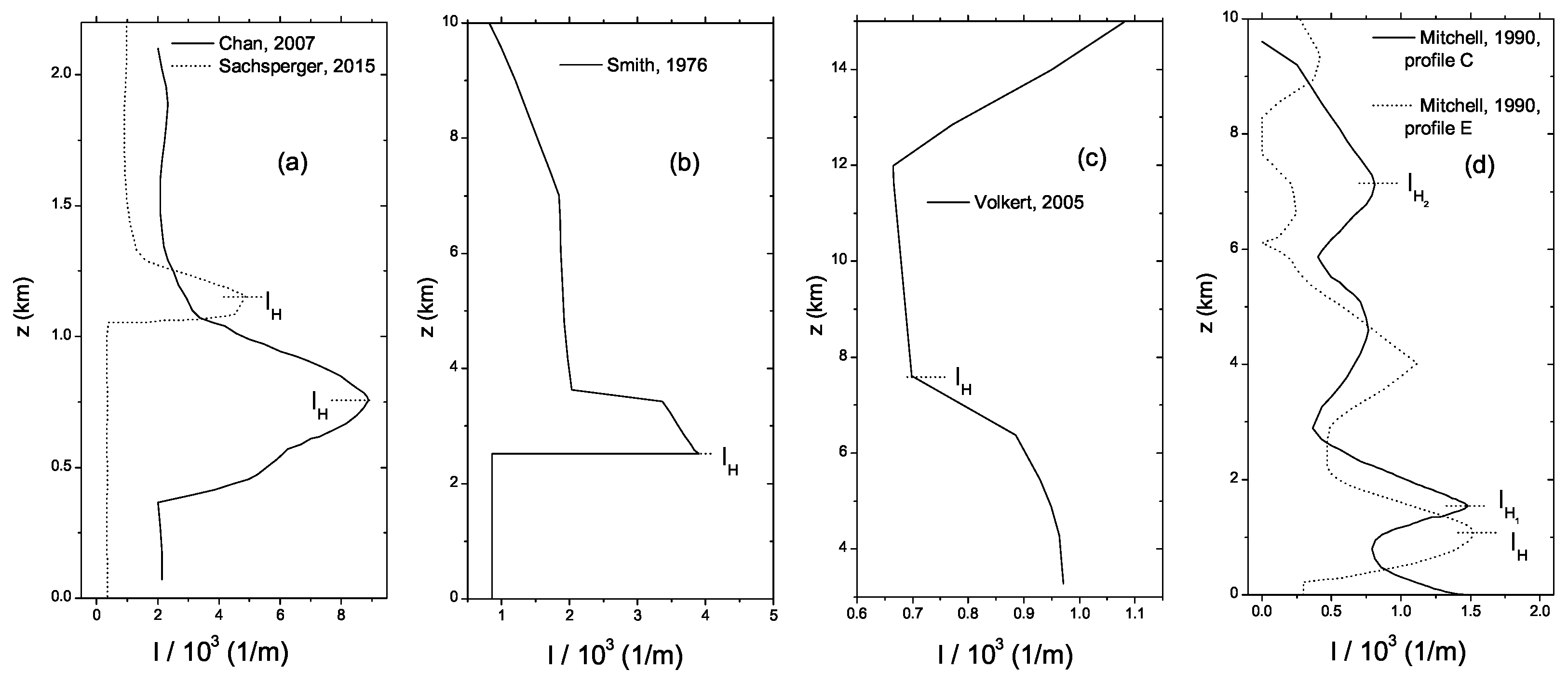
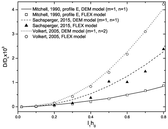
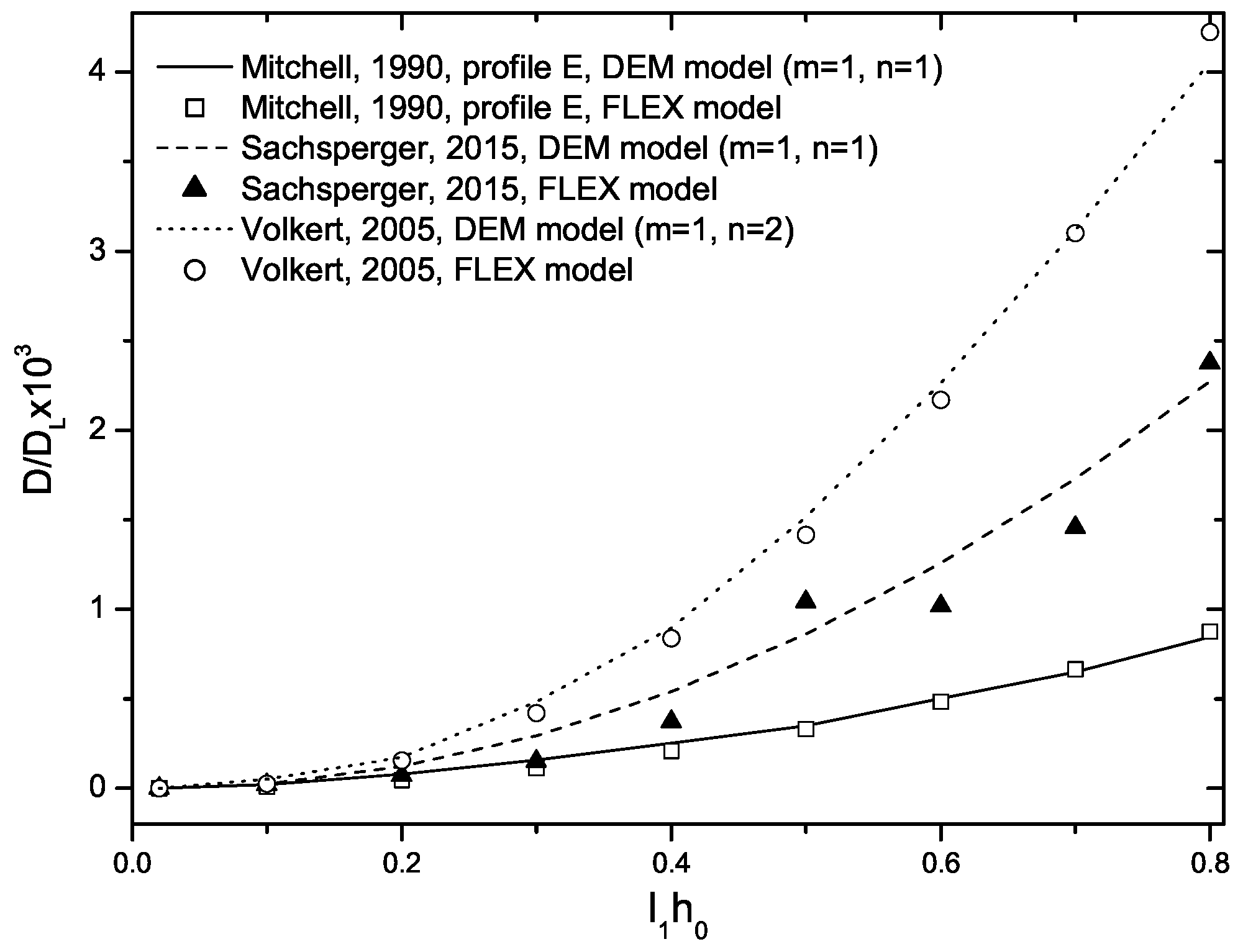
Figure 7 and Figure 8 compare $D/D_L({\widehat{h}}_0)$ results from FLEX and DEM for the observational cases. Except for the [27] case and profile C [20], both models show high consistency. Profile C [20] is the most complex ($m=2,n_1=n_2=1$), with discrepancies appearing only for ${\widehat{h}}_0>0.7$ while maintaining robust overall agreement. For the [27] case, numerical scatter complicates validation, though the DEM follows the general trend of the simulations. Overall, these results confirm the reliability of the DEM across diverse atmospheric conditions, ranging from moderate-to-strong non-hydrostatic regimes.

Figure 7. $D/D_L({\widehat{h}}_0)$ profiles obtained using the FLEX and DEM models for the observational $l\left(z\right)$ profiles reported by [19,20,21]. Profile C refers to the data from [20].

Figure 8. As in Figure 7 but for the observational $l\left(z\right)$ profiles from [20,22,27]. Profile E refers to the data from [20].

Limitations and Applicability of DEM

The DEM assumes a 2D, inviscid, non-rotating flow, where the BL is either negligible or the waves of interest reside above the friction-dominated region. While the real atmosphere features a BL up to 1 km, an inviscid free-slip lower boundary is physically consistent for scenarios where its influence on wave generation is secondary.

Following the analysis of Argain [18], this inviscid configuration precludes wave breaking and classical rotors, which are intrinsically linked to friction and no-slip conditions. In their absence, the system responds via internal mechanisms: duct resonance detuning, harmonic generation, and leakage into propagating waves. These processes typically lead to drag saturation or redistribution rather than sharp monotonic increases.

However, TLW and rotors are often interconnected, neglecting friction removes a key momentum transfer pathway. Consequently, by suppressing friction, the DEM may either overestimate wave drag in rotor-prone regimes, or conversely, underestimate total drag in cases where friction-driven flow separation creates additional form drag (e.g., wake effects). Despite this, the model remains a robust tool for a wide range of realistic atmospheric scenarios. The relevance of such internal-wave dynamics in the free atmosphere, far from surface frictional effects, is exemplified by recent observations and simulations of wave trapping occurring even at high altitudes, such as near the tropopause (e.g., [28]).

Note that the accuracy of the DEM is contingent upon the correct identification of the dominant Scorer parameter maxima; thus, it is not recommended for flows where the Scorer parameter vertical structure is poorly defined or highly transient.

6. Conclusions

This study introduces and validates DEM, a parametric framework for estimating total pressure drag, as a function of non-linearity ($D({\widehat{h}}_0)$), in moderate-to-strong non-hydrostatic flows, characterized by TLW. By leveraging the two-layer Scorer atmosphere as a physical baseline, the DEM provides a computationally inexpensive alternative to high-resolution numerical simulations, offering a physically grounded approach to drag estimation in realistic atmospheric conditions.

The primary contributions of this work are threefold:

• Normalization Strategy: Normalizing total drag by its linear counterpart ($D_L$, obtained via DLM) provides a robust unifying framework. Since $D_L$ is efficiently calculated with negligible computational cost, this approach effectively collapses the complex dependence of drag on non-linearity ($D({\widehat{h}}_0)$) into a set of non-linear correction functions suitable for real-time applications. These functions are defined by the mode number n, the duct depth H, and the Scorer parameter at the interface ($z=H$).
• Modal Dependence: Non-linear drag enhancement in the presence of TLW is critically dependent on the mode number n. While the fundamental mode ($n=1$) largely maintains the quadratic mountain-height scaling characteristic of linear theory, higher-order modes exhibit marked divergence as non-linearity increases. The DEM successfully accounts for this behavior through its mode-dependent formulation.
• Validation and Robustness: The model demonstrates strong agreement with FLEX numerical simulations across a diverse range of soundings. The high consistency of the DEM across the majority of the cases investigated suggests that, in scenarios where numerical simulations exhibit instability, the empirical model provides a more physically consistent representation of the drag trend, effectively bypassing numerical artifacts associated with near-singular resonance zones.

By capturing realistic trends such as resonance and saturation under non-linear conditions, the DEM provides a robust strategy for improving orographic drag parameterizations in weather and climate models. Its implementation can significantly reduce the computational overhead of resolving non-hydrostatic effects over steep terrain. Future research should incorporate surface friction and three-dimensional topographic effects to further extend the applicability and realism of this empirical framework.

References

- Phillips, D.S. Analytical surface pressure and drag for linear hydrostatic flow over three-dimensional elliptical mountains. J. Atmos. Sci. 1984, 41, 1073–1084. [Google Scholar] [CrossRef] [Scilit]
- Shutts, G.J.; Gadian, A. Numerical simulations of orographic gravity waves in flows which back with height. Q. J. R. Meteorol. Soc. 1999, 125, 2743–2765. [Google Scholar] [CrossRef] [Scilit]
- Smith, R.B. The influence of mountains on the atmosphere. Adv. Geophys. 1979, 21, 87–230. [Google Scholar] [CrossRef] [Scilit]
- Teixeira, M.A.C.; Miranda, P.M.A. A linear model of gravity wave drag for hydrostatic sheared flow over elliptical mountains. Q. J. R. Meteorol. Soc. 2006, 132, 2439–2458. [Google Scholar] [CrossRef] [Scilit]
- Lilly, D.K.; Klemp, J.B. The effects of terrain shape on nonlinear hydrostatic mountain waves. J. Fluid Mech. 1979, 95, 241–261. [Google Scholar] [CrossRef] [Scilit]
- Smith, R.B. Hydrostatic airflow over mountains. Adv. Geophys. 1989, 31, 1–41. [Google Scholar] [CrossRef] [Scilit]
- Durran, D.R. Mountain Waves and Downslope Winds. In Atmospheric Processes over Complex Terrain; Meteorological Monographs; American Meteorological Society: Boston, MA, USA, 1990; Volume 23, pp. 59–81. [Google Scholar]
- Ólafsson, H.; Bougeault, P. Nonlinear flow past an elliptic mountain ridge. J. Atmos. Sci. 1996, 53, 2465–2489. [Google Scholar] [CrossRef] [Scilit]
- Miranda, P.M.A.; James, I.N. Non-linear three-dimensional effects on gravity-wave drag: Splitting flow and breaking waves. Q. J. R. Meteorol. Soc. 1992, 118, 1057–1081. [Google Scholar]
- Teixeira, M.A.C.; Argain, J.L.; Miranda, P.M.A. Drag produced by trapped lee waves and propagating mountain waves in a two-layer atmosphere. Q. J. R. Meteorol. Soc. 2013, 139, 964–981. [Google Scholar]
- Teixeira, M.A.C.; Argain, J.L.; Miranda, P.M.A. Orographic drag associated with lee waves trapped at an inversion. J. Atmos. Sci. 2013, 70, 2930–2947. [Google Scholar] [CrossRef] [Scilit]
- Peltier, W.R.; Clark, T.L. Nonlinear mountain waves in two and three spatial dimensions. Q. J. R. Meteorol. Soc. 1983, 109, 527–548. [Google Scholar] [CrossRef] [Scilit]
- Lott, F. A New Theory for Downslope Windstorms and Trapped Mountain Waves. J. Atmos. Sci. 2016, 73, 3585–3597. [Google Scholar] [CrossRef] [Scilit]
- Vosper, S.B. Inversion effects on mountain lee waves. Q. J. R. Meteorol. Soc. 2004, 130, 1723–1748. [Google Scholar] [CrossRef] [Scilit]
- Doyle, J.D.; Coauthors. An intercomparison of T-REX mountain-wave simulations and implications for mesoscale predictability. Mon. Weather Rev. 2011, 139, 2811–2831. [Google Scholar]
- Scorer, R.S. Theory of waves in the lee of mountains. Q. J. R. Meteorol. Soc. 1949, 75, 41–56. [Google Scholar] [CrossRef] [Scilit]
- Lott, F. A study of the low frequency inertio-gravity waves observed during PYREX. J. Geophys. Res. 1998, 103, 1747–1757. [Google Scholar]
- Argain, J.L. Pressure drag produced by trapped lee waves and propagating mountain waves under nonlinear conditions. EGUsphere 2026, preprint. [Google Scholar] [CrossRef] [Scilit]
- Smith, R.B. The Generation of Lee Waves by the Blue Ridge. J. Atmos. Sci. 1976, 33, 2548–2560. [Google Scholar] [CrossRef] [Scilit]
- Mitchell, R.M.; Cechet, R.P.; Turner, P.J.; Elsum, C.C. Observation and Interpretation of Wave Clouds over Macquarie Island. Q. J. R. Meteorol. Soc. 1990, 116, 741–752. [Google Scholar] [CrossRef] [Scilit]
- Chan, P.W. Atmospheric Waves Associated with a Valley of Lantau Island: Observation, Theory and Numerical Simulation. In Proceedings of the 12th Conference on Mesoscale Processes, American Meteorological Society, Waterville Valley, NH, USA, 6–9 August 2007; American Meteorological Society: Boston, MA, USA, 2007; Paper 122547. [Google Scholar]
- Volkert, H.; Collaborators, E. Physical Background of Lee Waves: Trapped versus Vertically Propagating. In EUMETRAIN Training Modules; Consortium, E., Ed.; EUMETRAIN/DLR: Oberpfaffenhofen, Germany, 2005; Chapter IV. [Google Scholar]
- Argain, J.L.; Miranda, P.M.A.; Teixeira, M.A.C. Estimation of the friction velocity in stably stratified boundary layer flows over hills. Bound.-Layer Meteorol. 2009, 130, 15–28. [Google Scholar]
- Teixeira, M.A.C.; Miranda, P.M.A. Linear criteria for gravity-wave breaking in resonant stratified flow over a ridge. Q. J. R. Meteorol. Soc. 2005, 131, 1815–1820. [Google Scholar]
- Teixeira, M.A.C.; Miranda, P.M.A.; Argain, J.L. Mountain waves in two-layer sheared flows: Critical level effects, wave reflection, and drag enhancement. J. Atmos. Sci. 2008, 65, 1912–1926. [Google Scholar] [CrossRef] [Scilit]
- Doyle, J.D.; Reynolds, C.A. Implications of Regime Transitions for Mountain-Wave-Breaking Predictability. Mon. Weather Rev. 2008, 136, 5211–5223. [Google Scholar]
- Sachsperger, J.; Serafin, S.; Grubišić, V. Lee Waves on the Boundary-Layer Inversion: Their Dependence on Atmospheric Stability. Front. Earth Sci. 2015, 3, 70. [Google Scholar]
- Dörnbrack, A. Transient tropopause waves. J. Atmos. Sci. 2024, 81, 1647–1668. [Google Scholar] [CrossRef] [Scilit]
Disclaimer/Publisher’s Note: The statements, opinions and data contained in all publications are solely those of the individual author(s) and contributor(s) and not of MDPI and/or the editor(s). MDPI and/or the editor(s) disclaim responsibility for any injury to people or property resulting from any ideas, methods, instructions or products referred to in the content. |
© 2026 by the author. Licensee MDPI, Basel, Switzerland. This article is an open access article distributed under the terms and conditions of the Creative Commons Attribution (CC BY) license.