


Abstract
This study presents a novel detailed mathematical model of vibrational relaxation in pure methane. Based on the critical analysis of the available experimental data, a new kinetic scheme of vibrational energy exchanges is constructed. A reduced five-process scheme for the bending modes is proposed for comparison with experiments. The state-to-state rate coefficients of vibrational–translational (VT) and vibrational–vibrational (VV) processes are calculated on the basis of the forced harmonic oscillator (FHO) model, which is for the first time applied to CH4–CH4 collisions in a unified two-oscillator formulation covering intermolecular and intramolecular energy exchanges. The model parameters are calibrated against experimental relaxation times in the temperature range 140–1100 K. The state-to-state, three-temperature, and two-temperature descriptions of the bending mode relaxation are assessed by solving the isothermal bath problem. It is shown that the three-temperature model yields excellent agreement with the state-resolved solution for the relaxation time. The two-temperature model is valid mainly for moderate and high temperatures. The roles of individual energy transitions in the relaxation are identified, the VT deactivation of the triply degenerate bending mode dominating the relaxation.
1. Introduction
Methane attracts considerable attention nowadays in planetary science, atmospheric physics, and spectroscopy. It is a key component of the atmosphere of Titan, explored by the Cassini–Huygens mission [1,2] and targeted by the planned Dragonfly mission [3], and of the ice-giant atmospheres considered for future in situ exploration [4]. Accurate knowledge of the methane spectrum, including transitions between excited vibrational states, is necessary for the reliable detection of CH4 in planetary and exoplanet atmospheres [5,6,7], and the interpretation of the observed emission depends on the non-equilibrium populations of the vibrational states [8,9]. Non-equilibrium spectra of methane are also studied in laboratory hypersonic flows [10]. Vibrational relaxation directly affects the laser-based photoacoustic detection of atmospheric methane [11]. In the Earth atmosphere, methane is the second most important anthropogenic greenhouse gas after carbon dioxide [12,13]. In all these fields, vibrational energy transitions play an important role. However, the description of the methane vibrational kinetics remains rather limited.
Vibrational relaxation times in methane and its mixtures were measured in numerous experimental studies [14,15,16,17,18,19,20,21,22,23]. Early measurements showed that, despite the four distinct vibrational modes of the CH4 molecule, the gas can be attributed with a single relaxation time, commonly interpreted as an indication of rapid mutual equilibration of the bending modes [14,15]. Later state-selective experiments [24,25,26,27,28,29] resolved individual channels of VT and VV energy exchange, established the staged character of the relaxation with the slow deactivation of the bending modes, and provided elementary rate coefficients for several transitions between the lowest vibrational levels. Nevertheless, the data remain rather scattered: the relaxation times reported near room temperature disagree by almost a factor of two, the state-resolved rates are available only near room temperature, and the low- and high-temperature ranges are covered sparsely.
Theoretical modeling of the methane vibrational kinetics is much less developed than that of other polyatomic gases, such as carbon dioxide [30,31,32,33,34,35]. In plasma chemistry, detailed kinetic models of methane conversion were constructed [36,37], and vibrationally excited CH4 states were explicitly included in [38], following the level schemes developed for CO2 plasmas [39,40]. In such models, the vibrational kinetics is reduced to a small number of effective levels, and the rate coefficients of vibrational transitions are evaluated from approximate scaling relations. Growing attention is also paid to flows of methane–nitrogen mixtures associated with entry into the Titan atmosphere. Thermochemical kinetic models of such flows were proposed in [41,42], new shock-tube benchmarks have been reported recently [43,44], and continuum and direct simulation Monte Carlo studies of the entry conditions were performed [45]. Recently, the multi-temperature and state-to-state descriptions were applied to the Titan atmospheric entry [46]. In the fluid-dynamic models, vibrational relaxation is described by phenomenological correlations [21,47] fitted to a limited set of data. In our previous work [48], a self-consistent one-temperature model of methane flows was developed and applied to the shock-wave structure, with the vibrational relaxation time evaluated from the correlation [21]. Thus, the existing descriptions either treat the vibrational energy reservoir as a whole or are restricted to transitions between the lowest vibrational states. To the authors’ knowledge, a kinetic scheme following from the experimentally observed transitions, supplemented with a consistent set of state-resolved rate coefficients, has not yet been developed for methane.
Constructing such a scheme requires theoretical models of the rate coefficients since higher vibrational states become populated with increasing temperature and degree of non-equilibrium, whereas the experiments mostly probe small perturbations of the equilibrium state and transitions between the first excited levels. The observed processes therefore have to be generalized to higher vibrational levels, and the complete set of state-to-state (STS) rate coefficients has to be reconstructed from the limited measured data. For polyatomic molecules, two semiclassical models are commonly employed, the Schwartz–Slawsky–Herzfeld (SSH) model [49] and the forced harmonic oscillator model [50,51]. In the first-order SSH formulation, only single-quantum transitions are allowed, and the computed probabilities may exceed unity at high temperatures. The corresponding perturbation integrals were evaluated for methane already in the early studies [52,53], and the SSH-type calculations were later extended to polyatomic gases [54].
The FHO model is based on the exact solution for a harmonic oscillator forced by a classical trajectory [55,56], extended to two oscillators exchanging quanta [57]. It allows for multi-quantum transitions within a single collision, employs the symmetrized collision velocity consistent with detailed balance, and accounts for the non-collinear collision geometry through empirical steric factors [50]. A three-dimensional extension free of empirical steric factors was also developed (FHO-FR) [51]. For polyatomic molecules, the FHO model was applied to CO2 and its mixtures, with the mode parameters obtained from the normal-mode analysis and the intermolecular exchanges taken into account [32,58,59,60].
For methane, the applicability of the SSH-type models is known to be limited: the comparison with the measured deactivation rates showed disagreement by orders of magnitude [61]. The FHO model, which avoids the single-quantum and unbounded-probability limitations of the first-order treatment, has not yet been applied, to the authors’ knowledge, to CH4–CH4 collisions. Developing the FHO-based description of vibrational energy transitions in pure methane is the main goal of the present study. Such a description closes the kinetic scheme constructed from the experimentally observed transitions, for which state-resolved rate coefficients have not been available so far. It thereby extends the modeling of methane flows beyond the one-temperature approach of our previous work and makes it possible to formulate the state-to-state and multi-temperature fluid-dynamic models on a consistent kinetic basis.
The objectives of the present study are the following: (1) to analyze the available experimental data on vibrational energy transitions in CH4–CH4 collisions and to construct a new kinetic scheme of VT and VV processes; (2) to extend the FHO model to CH4–CH4 collisions in a unified formulation covering intermolecular and intramolecular energy exchanges; (3) to calibrate the model parameters against the measured bending relaxation times; (4) to develop advanced closed fluid-dynamic models of methane flows with vibrational relaxation in the state-to-state, three-temperature, and two-temperature approximations, taking into account different kinetic scaling; (5) to assess the reduced models against the state-resolved solution of the isothermal bath problem; and (6) to identify the roles of individual processes in the relaxation of the bending modes.
The paper is organized as follows. In Section 2, we carry out a critical analysis of the experimental data on vibrational energy transfer in CH4–CH4 collisions and select the processes governing the relaxation of the bending modes. The experimental data on the VV exchanges and the complete kinetic scheme are written in Appendix A and Appendix B, respectively. Section 3 presents the closed systems of governing equations in the state-to-state and two multi-temperature approaches. In Section 4, the FHO model is applied to CH4–CH4 collisions, and the calculated VV rate coefficients are compared with the measured ones. Section 5 presents the calibration of the model parameters and the assessment of the STS and MT in the isothermal bath problem. Concluding remarks are provided in Section 6.
2. Vibrational Energy Transfer in CH4–CH4 Collisions
In this section, we analyze the available experimental data on vibrational energy transitions in methane, identifying the main channels of vibrational energy relaxation. The data are then used to construct a kinetic scheme that reflects the processes observed in the experiments, generalized to higher vibrational levels of the methane molecule. The scheme itself is presented in Appendix B.
2.1. Vibrational Spectrum of Methane Molecule
Before discussing the experimental data in detail, let us first summarize the main features of the methane molecule and the assumptions on its spectrum adopted in the present work. Methane is a nonlinear five-atom molecule possessing three rotational and nine vibrational degrees of freedom. In this study, a quasi-classical description is adopted: the translational motion is treated classically, whereas the rotational and vibrational degrees of freedom are assumed to be quantized.
The rotational energy is assumed to be independent of the vibrational state and is evaluated in the rigid-rotor approximation. Since CH4 is a spherical-top molecule belonging to the point group, all three principal moments of inertia are equal, which leads to a comparatively simple structure of rotational levels [62].
The methane molecule has four normal vibrational modes that differ in symmetry and degeneracy as illustrated in Figure 1 and summarized in Table 1. Modes and correspond to the symmetric and antisymmetric C–H stretching vibrations, whereas modes and represent the bending deformations. The lowest-frequency mode is , followed by , while both stretching modes are characterized by considerably higher vibrational quanta. This frequency ordering indicates that the bending subsystem is expected to dominate the direct vibration–translation relaxation, whereas the stretching modes relax primarily through vibration–vibration energy redistribution.
Figure 1.
Normal vibrational modes of the methane molecule. The arrows indicate the relative atomic displacements.
Table 1.
Spectroscopic constants of the normal vibrational modes of methane.
Within the harmonic-oscillator approximation, the vibrational energy of a methane molecule in the vibrational state is written as [62]
where h is the Planck constant, c is the speed of light, is the spectroscopic constant of mode m related to its frequency, is the degeneracy of the mth mode, and is the corresponding vibrational quantum number. For the dissociation energy J, this model yields 1935 vibrational states below the dissociation threshold [48].
Due to the degeneracy of the bending (, ) and antisymmetric stretching () modes, each vibrational state has a statistical weight [48]
which accounts for the number of degenerate sub-states sharing the same vibrational energy (1).
The harmonic-oscillator approximation (1) is adopted in the present work. Second-order perturbative approaches to vibrational anharmonicity have been developed for polyatomic molecules, including analytical formulations for linear and symmetric-top molecules [64] and perturb-then-diagonalize treatments applicable to spherical tops such as methane [65,66]. Their application to the present vibrational-energy model would require the determination of the corresponding molecule-specific parameters and an additional treatment of degeneracy and resonance effects. The inclusion of anharmonicity is therefore left for future work, where both the calculation of anharmonic constants and the use of vibrational energies available from variational or spectroscopic studies [6,67,68] may be considered.
2.2. Vibrational Energy Transitions in Methane Collisions
We now specify the types of vibrational energy transitions considered in this work. Since pure single-component methane is studied, all collisions are those of two CH4 molecules. In a binary collision, and denote the vibrational states of the colliding molecules, and the primed symbols denote the post-collision values. In the VT transitions, the partner state does not change, and the exchange occurs for the specific mode only, e.g.,
In the VV exchanges, either both partners change their vibrational states, or energy exchange occurs between different modes of a polyatomic molecule. The VV transitions are written as
The energy excess in the transition is transferred to the translational motion.
2.3. Experimental Data on VT Relaxation
Most of the available experimental data for pure methane are related to VT relaxation. The measurements were obtained by a variety of techniques, such as ultrasonic absorption and velocity-dispersion measurements [14,15,16,17,18,19,20,69], shock-tube vacuum-ultraviolet absorption [21], laser-induced vibrational fluorescence [24,61], photoacoustic and spectrophone phase-shift techniques [22,23,27,70], and time-resolved pump–probe double-resonance measurements [28,29]. Figure 2 summarizes the experimental data on the pressure-normalized vibrational relaxation time in pure methane gas [14,15,16,17,18,19,20,22,23,24,25,27,28,29,61,69,70,71,72,73].
Figure 2.
Experimental data on VT relaxation times in pure methane [14,15,16,17,18,19,20,21,22,23,24,25,27,28,29,61,69,70,71,72,73].
At moderate temperatures, the data obtained by different techniques follow a common trend, although the values reported near room temperature can still disagree by almost a factor of two. At low and high temperatures the data are much sparser and the uncertainty is correspondingly higher. In the same figure we also show the phenomenological model of Millikan–White [47], in which the relaxation time is evaluated from the characteristic vibrational temperature of the mode with the lowest frequency, together with the model of Richards and Sigafoos [21] adopted in our previous work [48]. The Millikan–White model overestimates the relaxation time by more than an order of magnitude. The Richards–Sigafoos formula was fitted to shock-tube data and agrees with the data near and above room temperature, overestimating only at low temperatures.
In most experiments, the reported VT relaxation time corresponds to the relaxation of the bending subsystem rather than of an isolated mode since the modes and have similar frequencies and are efficiently coupled by VV redistribution [24,26,27,28,29]. Following common notation, the symbol is used throughout the paper for the mode m. Therefore, the observed VT relaxation is usually interpreted as the effective relaxation of the combined bending subsystem [23,24]:
where is the VT relaxation time of mode m, and is the equilibrium population of the first excited level of mode m at the translational–rotational temperature T [23,24] so that for the Boltzmann distribution,
Here, is the Boltzmann constant. In Figure 2, we assume that the experimental data correspond to this effective case, the only exception being the times reported for the third mode [25]. To further illustrate the inaccuracy of the Millikan–White formula, we also show its effective relaxation time calculated from Equation (5), which also deviates substantially from the measurements.
For the calibration of the FHO model parameters (Section 5), we will employ the bending-relaxation times of Boursier et al. [28,29], Hill and Winter [19], Wang and Springer [20], Parker and Swope [72], Avramides and Hunter [27], Eucken and Aybar [14], and Perrin et al. [22,23]. These works cover the whole temperature range 140–1100 K while avoiding duplicated data sets.
2.4. Experimental Data on VV Energy Exchanges
Experimental studies on VV exchanges in pure methane are much less common than those on VT transitions. The VV relaxation times were measured by Yardley and Moore [24], Vasconcelos and De Vries [70], Hess, Kung and Moore [26], Avramides and Hunter [27], and Boursier et al. [28,29]. Some of them were revised in Ref. [9]. Most of the measurements were performed near room temperature, so their conclusions apply mainly to the low- and moderate-temperature kinetics. The time values are summarized in Appendix A and are collected in Figure 3, grouped according to the type of process and the number of exchanged quanta.
Figure 3.
Experimental VV exchange rates in CH4–CH4 collisions near room temperature, grouped by process type [9,24,26,27,28,29,70].
In the compact notations of the processes, is the kth vibrational level of mode , and the tilde marks the modes of the collision partner. Thus, denotes the intermolecular exchange of the bending quanta, and the intramolecular one. Additionally, denotes an unresolved bending quantum ( or ), and marks totals over unresolved channels. Unless indicated otherwise, the transitions proceed mostly from the first excited level of the initial mode to the first excited levels of the resulting modes. Here, we mostly review the direct reactions (→) as reported in experiments, unless written otherwise.
The names of the processes in Figure 3 are adopted from the experimental works. The resonant transfer of a vibrational quantum to the same mode of the collision partner, , reported for the and modes, was denoted as “swap” in [28,29], and this designation is used throughout the paper. The term “sharing” refers to the transitions distributing the vibrational energy of the excited molecule between both collision partners. The label “mixed” marks the summary rates over unresolved channels.
The most rapid exchanges (see Figure 3) are those responsible for the intra-manifold equilibration, that is, the redistribution within the stretching subsystem and the redistribution within the bending subsystem. The values reported for the stretch–stretch energy exchange agree well and show that the two stretching modes can be treated as mutually equilibrated on the timescale of the slower channels. The data show larger scatter. Still, the small energy gap between the two bending modes and recent pump–probe measurements [28,29] indicate that this exchange is also rapid.
The resonant intermolecular exchange within the mode (the -ladder processes ) also has comparatively large rates that scale almost linearly with the level number. This shows that, once the energy enters the bending manifold, it is redistributed rapidly over the ladder of the levels.
The most important result of the analysis of VV measurements is the identification of the dominant stretch-to-bend energy transition channels. The direct single-quantum transition is slow because of its large energy release. The near-resonant double-quantum and combination pathways, such as or , are much more efficient and are expected to be the main channels towards the redistribution of energy between stretching and bending modes.
Overall, the analysis of experimental data shows that vibrational relaxation in methane proceeds in several distinct stages, consistently reported in [24,25,28,29]: (i) the rapid resonant and near-resonant exchanges first establish quasi-equilibrium within the stretching and within the bending manifolds; (ii) the stretch-to-bend transition channels then transfer energy between the manifolds on a distinctly longer timescale; and (iii) finally, the vibrational energy accumulated in the bending manifold is deactivated to translation through the slow VT processes. During the intermediate stages, the two manifolds may therefore have different vibrational temperatures.
Based on the above observations, we construct the kinetic scheme presented in Appendix B. The scheme includes the reactions observed in the experiments, generalized to higher vibrational levels, together with several additional processes. The next step is to identify the rate coefficients for the processes of the scheme.
In the present work, due to the large number of vibrational exchanges in methane, we start with a perturbation of the mode, following the conditions of most experiments. Five processes are considered: the VT relaxation of the two bending modes, VT2 (A2) and VT4 (A3); the intramolecular and intermolecular exchanges, and (A7); and the resonant quantum swap within the mode, (A8). The kinetic scheme contains an explicit swap for the mode only since no experimental rate is available for the analogue. The subsets of these processes retained in each fluid-dynamic model are specified in the next section, where the corresponding systems of governing equations are constructed.
3. Fluid-Dynamic Models for Describing Vibrational Relaxation of the Bending Modes
In this section, we present the closed systems of governing equations for non-equilibrium gas flows in pure methane, written for the state-to-state (STS) approach and for the reduced multi-temperature (MT) models within the generalized Chapman–Enskog method [74]. A closed one-temperature description of pure methane was considered in our previous work [48]. Here the three-dimensional systems are presented within the assumption of a vibrationally excited bending manifold. The vibrational excitation of the stretching modes and chemical reactions are neglected.
3.1. State-to-State Model
The STS formulation provides the most detailed flow description by treating the number density of each vibrational state as an independent macroscopic variable. The characteristic timescales within the reduced kinetic scheme are related as follows:
where and are the characteristic times of translational and rotational relaxation, is the characteristic time of the vibrational swaps within the mode, corresponds to the near-resonant exchange, is the VT relaxation time of the bending modes, and is the characteristic time of macroscopic parameter variation. Within the STS approach, only the equilibration of the translational and rotational degrees of freedom at the gas temperature T is used. The kinetic time-scale relation (7) allows one to specify the invariants of the most frequent collisions and to construct the closed system of governing equations [74]. The transport properties and relaxation terms can then be evaluated within the generalized Chapman–Enskog method. Details can be found in [74]. The system of governing equations reads [48,74]
where t is the time, and are the Cartesian coordinates. The vector of conservative variables and the vectors of convective fluxes , , have the form
The vectors of viscous fluxes and the source term vector are written as
Here, is the gas density, is the macroscopic velocity, is the pressure ( is the total number density, , m is the mass of a CH4 molecule), and the total energy per unit mass is defined as
The first row of (9) represents the equations for the state populations, and is the STS relaxation source term, which collects the contributions of the five processes of the kinetic scheme,
The explicit forms of the terms are specified in Section 3.4. The translational and rotational contributions to the energy are evaluated classically, and for nonlinear molecules
The rigid-rotor approximation and the Boltzmann distribution over rotational levels, combined with the small characteristic rotational temperature of the methane molecule, K, evaluated from the rotational constants reported in [62,75], allow the classical evaluation within the considered temperature range. The vibrational energy is calculated as the sum over the vibrational states,
with given by Equation (1). Since only the bending manifold is excited in the considered problems, the full set of 1935 vibrational states of methane is not required. The stretching modes are kept in their ground states, , because the processes by which they gain or lose quanta are not included in the kinetic scheme. The retained states with energies below the dissociation threshold form the 185-state domain.
The transport terms are the pressure tensor , the heat flux vector , and the diffusion velocities . The pressure tensor, which has the same form in all three models, is
where and are the shear and bulk viscosity coefficients, is the unit tensor, and is the relaxation pressure arising from the rapid inelastic RT exchanges and the slow inelastic processes [74]. Within the STS approach, the vibrational energy is transported by the diffusion of vibrational states. The diffusion velocity of molecules in state i and the heat flux are evaluated from [74]
Here, and are the state-resolved multicomponent diffusion and thermal diffusion coefficients, and is the thermal conductivity of the translational and rotational degrees of freedom.In this work, transport terms are not evaluated: the spatially homogeneous problems of Section 5 do not involve them.
3.2. Three-Temperature Model
The three-temperature model additionally assumes that the resonant exchanges within each bending mode are rapid:
The swaps conserve the number of vibrational quanta in each mode, so that the total numbers of and quanta thus become the additional collision invariants. Moreover, within the harmonic-oscillator assumption, the vibrational energy of each mode can replace the number of quanta as the invariant, and each mode acquires a Boltzmann distribution with its own vibrational temperature [30]. The non-equilibrium state is then described by three temperatures, T, , and . The 3T model is thus valid as long as the intra-mode exchanges remain faster than the inter-mode exchange and the VT relaxation, so that the populations within each mode retain the Boltzmann form. Its accuracy is verified against the state-resolved solution in Section 5.3. The governing equations retain the conservative form of the STS system (8), with two differences. The equations for the individual state populations are replaced by the single continuity equation for the gas density , and the system is supplemented with the relaxation equations for the mode vibrational energies,
where are the vibrational heat fluxes defined below, and and are the relaxation source terms:
The system is closed by the quasi-equilibrium distributions,
with being the vibrational statistical weight (2) evaluated with the stretching modes in their ground states (), is the partition function of the bending manifold evaluated over the retained set of states, and and are the energies of the first excited states. The mode vibrational energies, counted from the ground vibrational state, are
so that , the last term being the constant zero-point contribution. The vibrational heat capacities of the modes are introduced as the derivatives of the mode energies with respect to the corresponding vibrational temperatures, , . Mass diffusion vanishes in a single-component gas, and the vibrational energy is transported by the gradients of the vibrational temperatures:
where are the coefficients of vibrational energy transport, with in the present model and in the two-temperature model below. The pressure tensor retains the same form (15) as in the STS model.
3.3. Two-Temperature Model
The two-temperature model further assumes that the near-resonant exchange is also rapid:
The remaining vibrational invariant is the total number of bending quanta, and the two modes share a common bending temperature, . The 2T model therefore requires the inter-mode exchange to be faster than the VT relaxation of both modes, which restricts its applicability as assessed in Section 5.3 and Section 5.4. The distributions are given by Equation (21) with this constraint. The two vibrational energy equations (19) are replaced by a single equation for the combined bending energy ,
with the flux given by Equation (23). Only the two VT channels contribute to the source , each term being the corresponding mode contribution evaluated at (31). The vibrational heat capacity of the combined bending manifold is defined similarly, .
3.4. Relaxation Source Terms
The STS relaxation source term for state i under the , , and processes, in which only one molecule changes its vibrational state, can be written as
Here, is the state-to-state rate coefficient of process , under which state i changes to state . The backward coefficients follow from the detailed balance,
In the intermolecular processes and , both collision partners change their states, and the source term is written as follows:
where k and are the initial and final states of the partner. The backward coefficients follow from the detailed balance for the pair,
In the multi-temperature models, the energy source terms are obtained by the hybrid closure [31,32]: the STS production rates (26) and (28), evaluated with the quasi-equilibrium distributions (21), are summed with the corresponding vibrational energy,
In the 3T model, runs over the four processes of the sums (20). In the 2T model, the single source term is the sum of the two mode contributions,
A computationally cheaper closure employs the Landau–Teller expressions based on relaxation times. Within the multi-temperature approximation, each vibrational energy relaxes with a source term of the form
In the 3T model, corresponds to the two bending modes, with the relaxation times of the respective channels evaluated from the same rate coefficients (Section 5). In the 2T model, the combined bending energy relaxes through both VT channels, whose rates are additive. The Landau–Teller formulation is widely used in computational fluid dynamics. However, it is derived under the assumption of small deviations from equilibrium and loses accuracy under strongly non-equilibrium conditions [30,32,74].
In the present work, only spatially homogeneous relaxation problems are solved. The closure of the governing equations therefore reduces to evaluation of the state-resolved rate coefficients. Their construction for CH4–CH4 collisions on the basis of the FHO model is presented in the next section.
4. FHO Model Application for Methane Molecules
In this section, the forced harmonic oscillator (FHO) model [50,51,53,57] is extended to CH4–CH4 collisions to provide the state-to-state rate coefficients of vibrational energy transitions. The extension to methane is based on the structure of the model itself. The FHO probabilities are derived for an abstract harmonic oscillator driven by a classical trajectory. The molecule enters the model only through the mode frequency, the reduced oscillator mass, and the mass parameter, together with the interaction parameters and steric factors of the collision pair. Within the harmonic approximation adopted here, the vibrational motion of CH4 is represented by independent normal oscillators so that every mode can be treated as a forced harmonic oscillator to which the model applies directly. For methane, this mapping was introduced by Cottrell and Ream [53]. The remaining three-dimensional effects of the collision geometry are absorbed into the steric factors. These corrective factors were introduced for noncollinear collisions in Ref. [50] and are calibrated against rate data in the polyatomic applications [32,58] and in the present work. The main limitations of the resulting description should be kept in mind: the vibration–rotation Coriolis coupling, which is not negligible for the modes of a light and fast-rotating molecule, is not taken into account.
In the present work, both formulations of the FHO probabilities for polyatomic methane collisions are employed: the original Zelechow-type expressions, as in Ref. [58], and the simplified Bessel-function expressions of Adamovich et al. [50]. The choice between them for the VT and VV transitions is justified by direct comparison in Section 4.3.
4.1. Rate Coefficients from Integral Cross Sections
Consider a binary collision of two methane molecules, in which the vibrational states of the partners change in a VT (3) or VV (4) transition. The general state-to-state rate coefficient is given by [30,59,74]
where is the reduced mass of the collision pair, g is the relative velocity, and is its dimensionless counterpart. The integral scattering cross section is factored into the elastic and the inelastic parts [32,59]:
where is the elastic collision cross section of the pair and is the probability of the corresponding transition.
4.2. Elastic Collision Cross Section
The elastic collision cross section is calculated using the variable hard sphere (VHS) model [76]:
where the diffusion and viscosity cross sections are
The model parameters , , , and for CH4–CH4 interactions are obtained by fitting the VHS cross sections to the collision integrals computed from the Lennard–Jones potential with the methane parameters Å and K [77]. Their values are reported in Table 2. The fit is performed over the temperature interval 500–2000 K, so at the lower temperatures of the present study, down to 140 K, the power-law correlation is extrapolated beyond its fitting range.
Table 2.
VHS model parameters for CH4–CH4 interactions.
4.3. FHO Transition Probabilities
Here, we present the FHO expressions for the inelastic transition probabilities entering the factorization (34), first for the VT and then for the VV exchanges.
4.3.1. VT Transition Probability
For a VT-type transition (3), in which only the vibrational state of methane changes, the exact FHO probability follows from the closed-form solution for a harmonic oscillator forced by a classical trajectory [55,56]. For a transition within a single active mode m, it reads [58]
where the dimensionless FHO parameter represents the first-order perturbation theory (FOPT) probability of the fundamental single-quantum transition:
where and are the Morse potential parameters (the repulsion range parameter and the well depth), is the reduced oscillator mass for the active mode, is the mass parameter of the vibrational mode, and is the steric factor. The angle parameter is
The average oscillator frequency is computed from the vibrational energy change:
Here, s is the total number of exchanged vibrational quanta,
The symmetrized collision velocity is [50]
The original expression (37) was simplified by Adamovich et al. [50] into the Bessel-function form
where the combinatorial factor accounts for the multi-mode structure of methane [32]:
For the single-quantum VT transitions retained in the kinetic scheme, the two expressions give practically identical results: in our calculations, the rate coefficients computed from Equations (37) and (43) agree within over 140–1100 K for all retained transitions. The simplifiedform (43) is therefore used for the VT transitions.
4.3.2. VV Transition Probability
For a VV-type exchange (4), the original factorial probability was derived by Zelechow et al. [57] for two collinear harmonic oscillators carried by the colliding molecules. In this intermolecular form it was applied to the CO2–CO2 exchanges by Vargas et al. [58]. For the intramolecular transitions of CO2, in which one molecule changes several of its own modes while the partner only provides the perturbation, Kravchenko et al. [32] employed the single-oscillator VT expressions instead. Here, the two-oscillator construction is applied in a unified form to both configurations. The two exchanging oscillators are either the active modes of the two colliding molecules (intermolecular exchanges) or two effective oscillators of one molecule (intramolecular transitions).
Let the two exchanging oscillators change their states as (the oscillator losing quanta) and (the oscillator gaining quanta), and denote , . The probability reads
where , , , and are the orthogonal transformation matrices [57], which connect the product basis of the two oscillators with the normal-mode basis of the collision system. The parameter is given by Equation (38). The VV coupling parameter is
Here, is the VV steric factor. The symmetrized velocity in the VV case is evaluated by Equation (42), where the energy change is replaced by the net vibrational energy variation of the collision system .
The two configurations differ only in the assignment of the oscillators. In the intermolecular exchanges, the oscillators are the active modes of the two molecules, and is evaluated at the frequency of the mode losing quanta. In the intramolecular channels, the mode losing quanta forms the first oscillator. The resulting modes are combined into one effective oscillator, which carries their summed quanta and the oscillator mass of the mode gaining the most. The frequencies follow from the energy changes per exchanged quantum, in line with Equation (40), and is evaluated with the mass of the first oscillator at the frequency of the net energy variation , the energy actually exchanged with the translational motion. In both configurations, the steric factor applied to the -dependent (translational) factors is denoted and the one applied to is denoted .
In the regime , when the quantum exchange decouples from the translational motion, the sum reduces to the simplified expression [50]
with and being the combinatorial factors (44) computed for the two colliding molecules from their initial and final quantum numbers. Each factor is evaluated with the number of quanta exchanged by the corresponding molecule, and the exponent in Equation (47) is . The parameter accounts for near-resonant energy exchange:
For strictly resonant exchange (), and , so that the probability depends only on the parameter .
The two formulations are not equivalent for the VV exchanges. For the resonant intra-mode processes, the condition holds, and with the calibrated parameters of Section 5 the two formulations agree within . For the non-resonant inter-mode channels, the energy variation must be accommodated by the translational motion, the condition breaks down, and the predictions of the two formulations diverge by up to three orders of magnitude. The inaccuracy of the compact expressions for non-resonant multi-quantum VV transitions was noted already in Ref. [50]. Accordingly, the simplified formulation (47) is used for the resonant intra-mode exchanges, and the original construction for the non-resonant inter-mode channels.
4.4. Molecular Parameters for CH4–CH4 Collisions
The FHO model requires the following molecular parameters for each collision pair: the Morse interaction potential parameters (, ), the reduced oscillator masses (), the mass parameters (), the oscillator frequencies (), and the steric factors (, ). The mode frequencies are evaluated from the harmonic wave numbers listed in Table 1, which are the spectroscopic constants derived from the anharmonic force-field analysis of the measured vibration–rotation spectra of methane [63]. The values of the mass parameters and of the reduced masses can be calculated theoretically from the normal-mode analysis. The steric factors and Morse potential parameters require a fitting procedure since their values for the methane modes are not reported in the literature. The Morse parameters and the VT steric factors are fitted to the measured bending relaxation times in Section 5.2, and the VV steric factors are calibrated to the measured room-temperature rate coefficients in Section 4.5 and Section 5.4.
The reduced oscillator mass is the normal-mode reduced mass computed in the harmonic approximation [62,78]. For the () and (E) modes, the central carbon atom remains stationary by symmetry, and equals the hydrogen-atom mass exactly, whereas for the modes, the carbon atom displacement makes it slightly larger. For the latter modes, the reduced mass depends on the harmonic force field through the mixing of the two normal modes of the same symmetry, and closed-form expressions in terms of the atomic masses alone are only approximate. The values listed in Table 3 are therefore taken from the normal-mode calculation of the NIST database [79] (the harmonic normal-mode analysis at the Hartree–Fock/6-31G* level).
Table 3.
Vibrational mode parameters for CH4 used in the FHO model.
The mass parameter , evaluated theoretically from the normal-mode displacements, characterizes the fraction of the vibrational displacement carried by the atoms facing the collision partner. In methane, the vibrational displacement is carried almost entirely by the hydrogen atoms, and its projection onto the oscillation axis, averaged over the molecular orientations and the degenerate components of the mode, is close to for every mode: the value is exact for the and modes, in which the carbon atom is stationary, and deviates by less than for the modes. The value is therefore adopted for every mode as an effective orientation-averaged convention. The same value was used for all modes of CO2 in Refs. [32,58].
4.5. Calculated VV Rate Coefficients
Before employing the FHO model within the kinetic scheme, we illustrate that it yields VV rate coefficients of the correct magnitude and scaling for methane.
The calculations use the Morse parameters obtained in Section 5. The steric factors are calibrated per channel at the room-temperature reference rates. The processes accounted for include , , together with . The calibrated factors are collected in Table 4.
Table 4.
Calibrated steric factors of the resonant -ladder and stretch-to-bend VV channels; the channels of the original formulation share the factor .
Figure 4 shows the resonant quantum exchange within the mode, . For this resonant channel the two formulations coincide within one percent. The computed rates grow almost linearly with the level, reproducing the experimental scaling within the measurement uncertainty, and depend weakly on temperature. The measured rate at 193 K, however, exceeds the room-temperature value, whereas the model predicts a monotonic decrease and underestimates this point by almost a factor of two. A possible interpretation is that at low temperatures the resonant transfer becomes governed by the long-range attractive interaction, not described by the short-range repulsive FHO mechanism. A similar underestimation was reported for CO2 mixtures [32]. The FHO ladder rates should therefore be used with caution below 250 K.
Figure 4.
Rate coefficients of the resonant quantum exchange within the mode: dependence on the level at 296 K (left) and temperature dependence of the exchange (right) [9,28,29].
The non-resonant stretch-to-bend channels (Figure 5) are sensitive to the choice of the formulation. For , the original expression reproduces both measured temperatures, whereas the simplified one underestimates the 193 K rate by about and rises more steeply towards high temperatures. For , both formulations pass through the measured point by construction. The right panel shows the scaling with the stretching level, for which no measurements exist: the simplified expression grows roughly proportionally to , whereas the original one is almost independent of the level, and this difference remains the main open uncertainty of the extrapolation to highly excited states.
Figure 5.
Stretch-to-bend VV rate coefficients: temperature dependence of the and channels against the measured rates [26,28,29] and the fits of Ref. [9] (left). Dependence of the rate on the level at 296 K (right).
The simplified formulation remains accurate as long as the parameter is not too large, the underlying conditions being and [50]. For the VT transitions, they can be written as with
With the methane parameters, K for the mode and K for , so the conditions are satisfied. For the VV exchanges, however, the two formulations are equivalent only in the resonant channels (Section 4.3).
5. Results and Discussion
In this section, we present the results of fitting the FHO model parameters to the experimental data on vibrational relaxation in methane and assess the reduced fluid-dynamic models against the state-resolved description. The parameter calibration and the simulations are carried out for the kinetic scheme corresponding to bending-manifold relaxation. The calibration and the model comparisons of Section 5.2 and Section 5.3 employ the three-process set , , and , and the influence of the two remaining processes is examined in Section 5.4.
5.1. Procedures for Evaluating Vibrational Relaxation Times
To compare the predictions of the FHO model with the experimental data, the vibrational relaxation time must be rigorously defined and extracted from the kinetic equations. Three procedures are employed. The first two apply to the relaxation of the individual vibrational modes and processes, and the third defines the relaxation time for an arbitrary set of processes.
The first procedure provides a direct Landau–Teller estimate of the VT relaxation time of mode m through the rate coefficient of the fundamental VT transition, :
Here, is the characteristic vibrational temperature of mode m. The corresponding effective time of the bending manifold follows from Equation (5). The relation can also be used for the VV relaxation times, with the rate coefficient and energy of the fundamental VV transition, though such times are not directly comparable with the experimental data.
The second procedure follows from the kinetic theory [59,74]. Here, the relaxation time of a process with respect to a vibrational energy reservoir w is introduced through the averaging operator,
where is the specific heat of the subsystem, is the change of its energy in the transition, and denotes the averaging over the Maxwell distribution of the collision velocities and over the Boltzmann-weighted internal states of the partners with the cross section of process [59]. For the VT transitions, the formulation gives
The sum runs over the single-quantum deactivation transitions of the channel, is the equilibrium fraction of molecules in state i, and are the rate coefficients (33). For the combined bending relaxation time, the same expression is applied to the energy with the heat capacity (introduced in Section 3.3, here evaluated at equilibrium, ), the contributions of the two VT channels being additive.
Finally, the third and most general procedure extracts the relaxation time directly from the temporal evolution of the vibrational energy in an isothermal-bath simulation: the time is defined as the moment when the initial perturbation decays by a factor of e,
Unlike the first two procedures, the e-folding method is not restricted to the VT transitions. It operates on the computed energy evolution and therefore applies to any set of processes of the kinetic scheme. All values of the total bending time reported in this section are e-folding times, and the first two procedures provide the VT-based reference estimatescompared with them in Section 5.3. All isothermal-bath calculations of this section are performed at the pressure atm with the initial Boltzmann populations at K, unless stated otherwise.
5.2. Calibration of the FHO Model Parameters for the Bending-Manifold Relaxation
In this subsection, the FHO model parameters are fitted to the measured total bending relaxation times . The calibration set consists of 22 experimental points from the sources reviewed in Section 2 and covers the 140–1100 K temperature range. The objective function is the weighted sum of squared logarithmic deviations between the measured values and the model , extracted by the e-folding procedure (53) from the isothermal-bath solution of the STS system. The minimization is performed by the Nelder–Mead simplex algorithm in logarithmic variables and run to convergence.
Table 5 lists the resulting parameters. The calibrated model reproduces the 22-point set with a median deviation of . The largest residuals occur at 290–300 K, where the reported values themselves vary in the 1–2 μs·atm range and the fitted curve passes between them.
Table 5.
FHO parameters for the bending-manifold relaxation: , , and fitted to the total bending relaxation times, set by the 296-K closure , and the pair calibrated to Refs. [28,29].
The intramolecular exchange is described by the original formulation, whose probability carries two steric factors, in the translational () factors and in the VV () factor. They were calibrated at the fitted Morse parameters jointly to the two temperatures at which the rate coefficient is reported [28,29].
5.3. Differences Between STS and Multi-Temperature Formulations
We now assess the reduced multi-temperature descriptions of the bending-manifold relaxation against the state-resolved reference (8), with the FHO rate coefficients calculated with parameters from Table 5. Three reduced models are considered: the 3T and 2T models of Section 3 with the STS-averaged source terms (30), (31), and the 2T model closed by the Landau–Teller source terms (32) with the relaxation times evaluated from Equation (52).
Figure 6 compares the reduced models with the experimental data and shows their deviations from the state-resolved solution. The 3T model coincides with the state-resolved solution to better than over the whole range of 140–1100 K, and both 2T variants remain within , the kinetic-theory estimate (52) coinciding with the 2T Landau–Teller solution by construction. The Landau–Teller estimate (50) deviates within . The near-exact agreement of the 3T model is explained by the three-temperature distribution (21) capturing well the state-resolved populations.
Figure 6.
Reduced fluid-dynamic models of the bending-manifold relaxation: against the experimental data [14,15,16,17,18,19,20,22,23,24,25,27,28,29,61,69,70,71,72,73] (left) and the relative deviations of the reduced models and of the direct estimates from the STS solution (right).
5.4. Influence of the Rapid VV Processes
In this section we investigate the influence of VV exchanges on relaxation times and populations. First, we estimate the influence of the exchange in its intramolecular form, employed in the calculations of the previous subsections. The term affects the results only weakly (Figure 7). Under the symmetric initial conditions, switching it off changes the 3T e-folding time by at most at 140 K and by about or less above 300 K. To expose the role of the exchange directly, the initial mode temperatures are then set asymmetrically, one bending mode at 650 K and the other at 350 K, so that the energy of the overheated mode can leave it only through its own VT channel or through the exchange. With the exchange active, the mode temperatures converge on a sub-microsecond scale in both cases, whereas without it each mode relaxes independently, and the e-folding time changes by up to . For close perturbations of the modes, the exchange can therefore be neglected, which makes the 2T formulation applicable to the bending relaxation.
Figure 7.
Impact of the term in the 3T model: mode temperatures at K for different initial values of (left) and the effect on under symmetric excitation of the STS-averaged source terms (right).
We now examine the two remaining processes of the scheme, and . No previously calibrated parameter is changed: the VT and coefficients are those of Table 5, and the swap steric factor is taken from Table 4.
The steric factors of cannot be obtained directly since the measurements do not separate the intermolecular exchange from the intramolecular one [28,29]. Two limiting cases are therefore considered. In scenario (i), the steric pair calibrated for (Table 5) is applied to the intermolecular configuration without change. In scenario (ii), the factor is recalculated so that the intermolecular fundamental transition alone reproduces the measured coefficient (Table 6).
Table 6.
Calibrated steric factors of the process.
The additional processes do not influence the energy relaxation. At all seven sampled temperatures, switching on the swap and the intermolecular exchange , individually or together, changes by less than . This holds in the state-resolved and in the 3T descriptions, and for both calibration scenarios of (Figure 8). Distributing the measured exchange rate between the intramolecular and intermolecular configurations in any proportion changes by at most . The reason is that the intramolecular exchange alone equilibrates the mode temperatures three orders of magnitude faster than the VT decay.
Figure 8.
Relative change of upon inclusion of the additional processes, per model and calibration scenario: state-resolved (STS) solution (left) and 3T model (right).
The role of the intermolecular channel is more pronounced at the population level. Figure 9 shows the deviations of the state-resolved populations from the 3T distribution (21). The quoted deviations are the maxima attained beyond the initial rapid-exchange stage. At 300 K, the deviations reach for the three-process scheme since the intramolecular exchange conserves the sum and thus correlates the modes. Adding the intermolecular channel destroys this correlation, and the deviations drop to ( for the full five-process scheme shown in the figure), whereas adding the swap alone leaves them at about . At 1000 K, the deviations reach about for all variants of the scheme, at the -ladder states with . A state-resolved description is therefore required when these populations are of interest.
Figure 9.
Deviation of the state-resolved populations from the 3T distribution (21), for the three-process and the full five-process schemes at 300 K (left) and 1000 K (right).
The influence of the individual processes on the relaxation time is summarized in Figure 10, computed with the state-resolved solution of the five-process scheme. Removing any of the VV processes changes by less than . In contrast, removing increases by at 140 K and by at 1100 K, and removing increases it by a factor of 17 at 140 K and a factor of 3 at 1100 K. When both VT channels are removed, the relaxation cannot proceed, and the system retains 98– of the initial excess vibrational energy. The two intermolecular processes may therefore be omitted from the reduced energy descriptions, while the intramolecular remains the explicit coupling term of the 3T model.
Figure 10.
Removal of individual processes from the five-process scheme: the relative effect on (left) and the mode temperatures under the symmetric initial excitation K (right). The dotted line represents the bath temperature (300 K).
5.5. Numerical Efficiency of the Fluid-Dynamic Models
We now compare the computational cost of the state-resolved and MT descriptions in the isothermal bath problem, solved with identical initial data and the parameters of Table 5. Beyond the fluid-dynamic models, two sets of vibrational states are considered: the bending manifold, with the three-process scheme; and the full system of 1935 states, in which the kinetic scheme is supplemented with the relaxation channel, with the steric factors taken from Table 4. The reduced description of the full system is the 4T model, in which the quasi-equilibrium distribution (21) is supplemented by the common temperature of the stretching modes, maintained by the rapid resonant exchange. Table 7 lists the median values of calculation times over repeated single-thread runs at the seven sampled temperatures.
Table 7.
Time of the isothermal bath solution.
For the bending manifold, the costs of the two descriptions are comparable, and the 2T Landau–Teller model with the precomputed relaxation time requires less than a millisecond. For the full system, the state-resolved solution becomes roughly 10–20 times more expensive than in the 4T approximation, and the gain increases with the size of the state-resolved system: for carbon dioxide, the cost ratio of the state-resolved and hybrid multi-temperature descriptions is estimated as 80–100 [32]. The accuracy of the reduced description is retained, within for the bending manifold and within for the full system with the adopted set of parameters and the symmetric initial excitation. Since the parameters of the stretch-mode channels are evaluated at room temperature only, the full-system comparison serves primarily as a cost assessment. In multi-dimensional simulations, where transport coefficients have to be computed at each step and the number of variables dominates the cost, the advantage of the reduced models increases further.
5.6. Regression Formula for VT Relaxation Time
To provide an accessible correlation for CFD and kinetic-modeling applications [80], the state-resolved relaxation times of the bending manifold, computed with the parameters of Table 5 over 140–1100 K, are approximated by the empirical expression
Here, the term has the classical Landau–Teller form, and the additional term improves the description at low temperatures, where attractive interactions influence the measured times.
The fitted coefficients for the -excitation scheme are listed in Table 8, and the correlation reproduces the state-resolved results within over the considered temperature range.
Table 8.
Analytical regression coefficients for the modified Landau–Teller expression.
6. Conclusions
In this study, detailed models of non-equilibrium vibrational relaxation in pure methane were developed. The available experimental data on vibrational energy transitions in CH4–CH4 collisions were analyzed, and the observed VT and VV energy exchanges were classified according to the process type and the characteristic timescales. Based on this analysis, a general kinetic scheme was constructed by generalizing the observed transitions to arbitrary vibrational levels.
The state-to-state rate coefficients of the vibrational transitions were calculated using the FHO model, applied for the first time to CH4–CH4 collisions. We derived the required molecular parameters theoretically from the normal-mode analysis for methane–methane collisions. Two formulations of the transition probabilities were compared. It was shown that the simplified expressions can be applied to the VT transitions and to the resonant VV exchanges, whereas the non-resonant inter-mode channels require the original formulation. This distinction follows from the applicability conditions of the simplified formulation. For the VT transitions and the resonant exchanges, the two formulations practically coincide within the considered temperature range, whereas for the non-resonant channels, in which the energy variation has to be accommodated by the translational motion, the simplified expressions lose their accuracy, and the predictions of the two formulations differ by orders of magnitude. The model reproduces both the measured level dependence of the resonant exchange within the mode and the temperature dependence of the stretch-to-bend transitions. The unknown model parameters were calibrated by comparing the relaxation times obtained from the solution of the isothermal bath problem within the STS approach with the measured bending relaxation times, and the calibrated model reproduces the experimental data with satisfactory accuracy over a wide temperature range.
The closed systems of governing equations for non-equilibrium methane flows with excited bending manifold were presented in the state-to-state, three-temperature, and two-temperature approaches, continuing our previous one-temperature description. We assessed the reduced models with different closures of the relaxation terms against the state-resolved solution of the isothermal bath problem. It was shown that the three-temperature model yields excellent agreement with the state-resolved solution for the relaxation time. For the full system of vibrational states, the mode-temperature description with the additional stretching temperature is roughly an order of magnitude computationally cheaper than the state-resolved one, whereas for the bending manifold the costs of the two descriptions are comparable. The two-temperature model together with the Landau–Teller closure also provides good accuracy, with the largest deviations observed at low temperatures. The state-resolved populations remain close to the quasi-equilibrium 3T distribution, although noticeable deviations are found at the highly excited states of the mode. We also demonstrated that the VT deactivation of the mode dominates the relaxation, whereas the rapid VV exchanges affect the relaxation time only weakly. To summarize, the obtained results indicate that the bending-mode relaxation can be described with a common vibrational temperature of the bending modes.
Future work may include several directions. The next step is the modeling of the stretch-to-bend relaxation, which requires the calibration of the stretch-mode channels of the kinetic scheme. We also plan to extend the developed approach to methane-containing mixtures common in applications of methane flows, in particular CH4/N2, which is of interest for the planned missions to Titan. Refining the model at low temperatures and accounting for the vibration–rotation coupling and for the anharmonicity of the vibrational states are among other promising directions.
Author Contributions
Conceptualization, L.S.; methodology, L.S., E.K. and Z.M.; software, L.S. and Z.M.; validation, L.S. and Z.M.; formal analysis, L.S., E.K. and Z.M.; optimization, Z.M.; writing—original draft preparation, L.S. and Z.M.; writing—review and editing, E.K. and L.S.; supervision, E.K.; funding acquisition, E.K. All authors have read and agreed to the published version of the manuscript.
Funding
The work of L.S. and E.K. was supported by the Russian Science Foundation, project No. 23-19-00241-P.
Institutional Review Board Statement
Not applicable.
Informed Consent Statement
Not applicable.
Data Availability Statement
The data that support the findings of this study are available from the corresponding author upon reasonable request.
Conflicts of Interest
The authors declare no conflicts of interest.
Abbreviations
The following abbreviations are used in this manuscript:
| FHO | Forced Harmonic Oscillator |
| VT | Vibrational–Translational |
| VV | Vibrational–Vibrational |
| RT | Rotational–Translational |
| 1T | One-Temperature |
| MT | Multi-Temperature |
| STS | State-to-State |
| LT | Landau–Teller |
Appendix A. Experimental Data on VV Energy Exchanges in Methane
This appendix collects the available experimental data on the VV energy exchange rates in pure methane, summarized in Table A1, Table A2, Table A3, Table A4, Table A5 and Table A6. The notation follows Section 2: denotes the kth vibrational level of mode , and a prime marks a quantum belonging to the collision partner; most of the reported transitions involve only the first excited levels of the modes. For the entries whose individual channel is resolved by the experiment, the transition is additionally specified in terms of the vibrational states ; entries labeled “total” or “combined” refer to sums over channels not resolved by the experiment. The collision partner is shown only when it changes its state.
For each process , we list the pressure-normalized relaxation time and the rate coefficient . Depending on the source, the relaxation time is measured directly, derived from the observed signal decays, or inferred through the kinetic modeling of the experiment. The rate coefficient is related to by the approximate formula employed in Refs. [9,24,26,27,28,29,70]:
Table A1.
Experimental VV data from [24], laser-excited infrared fluorescence technique; K.
Table A2.
Experimental VV data from [70], optic-acoustic phase-lag measurements; K.
Table A3.
Experimental VV data from [27], optic-acoustic phase-shift measurements; K.
Table A4.
Experimental VV data from [26], laser-excited infrared fluorescence method; K.
Table A5.
Experimental VV data from [28,29], time-resolved infrared double-resonance technique; and 193 K.
The analysis of the data collected in Table A1, Table A2, Table A3, Table A4, Table A5 and Table A6, including the identification of the dominant energy-exchange channels and of their timescales, is given in Section 2. Starting from the reactions presented here, Appendix B formulates the kinetic scheme of vibrational energy exchanges in pure methane, in which the observed transitions are generalized to arbitrary vibrational levels.
Table A6.
VV data from [9], collection of linear fits to the data of works [25,81].
Appendix B. Kinetic Scheme
This appendix provides the complete list of the VT and VV processes proposed for the kinetic modeling of vibrational relaxation in pure methane. The processes are grouped into the VT and VV types (3) and (4). The energy variations are evaluated with the harmonic wave numbers of Table 1. We emphasize that the scheme is approximate: the experiments reviewed in Section 2 mostly provide data on transitions between the first excited levels of the modes, and here we extend them to higher levels. The relative importance of the individual channels may therefore change at high levels of excitation and at elevated temperatures.
Appendix B.1. VT Transitions
Direct VT relaxation proceeds through the bending modes and . Both channels are retained since the two modes have different frequencies and hence different VT rates.
- , single-quantum vibrational–translational relaxation of the mode:
- , single-quantum vibrational–translational relaxation of the mode:
Appendix B.2. VV Transitions
The VV exchanges of the first group below are rapid compared with VT relaxation and keep the stretching and bending manifolds internally equilibrated.
- , intramolecular exchange of the stretching quanta, ( cm−1):
- , intermolecular exchange of the stretching quanta, ( cm−1):
- , intramolecular exchange of the bending quanta, ( cm−1):
- , intermolecular exchange of the bending quanta, ( cm−1):
- , resonant intermolecular quantum swap within a single mode, , ; the reaction is written below for , the swaps in the remaining modes being analogous:
All processes of this first group conserve the total numbers of stretching quanta, , and bending quanta, , of the colliding pair.
The second group comprises the slower processes that transfer energy from the stretching modes to the bending modes. The relaxation of is not listed separately, as it is rapidly equilibrated with through the exchange [26,27,28].
- , single-quantum transition ( cm−1):
- , double-quantum transition ( cm−1):
- , intermolecular sharing , with one of the two created quanta residing on the collision partner ( cm−1):
- , combination transition ( cm−1):
- , single-quantum transition ( cm−1):
- , intermolecular sharing ( cm−1):
- , intermolecular transition ( cm−1):
- , intermolecular transition ( cm−1):
In the present work, we consider only the excitation of the bending manifold and a simplified kinetic scheme comprising five processes: , , the two bending exchanges and , and the resonant swap . The other VV channels are not yet included in the kinetic model. Still, for some of them the rate coefficients are calculated based on the FHO model and compared with the available data, in order to assess whether the model is capable of reproducing them (see Section 4.5).
References
- Lebreton, J.P.; Witasse, O.; Sollazzo, C.; Blancquaert, T.; Couzin, P.; Schipper, A.M.; Jones, J.B.; Matson, D.L.; Gurvits, L.I.; Atkinson, D.H.; et al. An overview of the descent and landing of the Huygens probe on Titan. Nature 2005, 438, 758–764. [Google Scholar] [CrossRef] [Scilit] [PubMed]
- Fulchignoni, M.; Ferri, F.; Angrilli, F.; Ball, A.J.; Bar-Nun, A.; Barucci, M.A.; Bettanini, C.; Bianchini, G.; Borucki, W.; Colombatti, G.; et al. In situ measurements of the physical characteristics of Titan’s environment. Nature 2005, 438, 785–791. [Google Scholar] [CrossRef] [Scilit] [PubMed]
- Barnes, J.W.; Turtle, E.P.; Trainer, M.G.; Lorenz, R.D.; MacKenzie, S.M.; Brinckerhoff, W.B.; Cable, M.L.; Ernst, C.M.; Freissinet, C.; Hand, K.P.; et al. Science goals and objectives for the Dragonfly Titan rotorcraft relocatable lander. Planet. Sci. J. 2021, 2, 130. [Google Scholar] [CrossRef] [Scilit]
- Mousis, O.; Atkinson, D.H.; Cavalié, T.; Fletcher, L.N.; Amato, M.J.; Aslam, S.; Ferri, F.; Renard, J.B.; Spilker, T.; Venkatapathy, E.; et al. Scientific rationale for Uranus and Neptune in situ explorations. Planet. Space Sci. 2018, 155, 12–40. [Google Scholar] [CrossRef] [Scilit]
- Yurchenko, S.N.; Tennyson, J. ExoMol line lists—IV. The rotation–vibration spectrum of methane up to 1500 K. Mon. Not. R. Astron. Soc. 2014, 440, 1649–1661. [Google Scholar] [CrossRef] [Scilit]
- Rey, M.; Nikitin, A.V.; Tyuterev, V.G. Accurate theoretical methane line lists in the infrared up to 3000 K and quasi-continuum absorption/emission modeling for astrophysical applications. Astrophys. J. 2017, 847, 105. [Google Scholar] [CrossRef] [Scilit]
- Bell, T.J.; Welbanks, L.; Schlawin, E.; Line, M.R.; Fortney, J.J.; Greene, T.P.; Ohno, K.; Parmentier, V.; Rauscher, E.; Beatty, T.G.; et al. Methane throughout the atmosphere of the warm exoplanet WASP-80b. Nature 2023, 623, 709–712. [Google Scholar] [CrossRef] [Scilit] [PubMed]
- Appleby, J.F. CH4 nonlocal thermodynamic equilibrium in the atmospheres of the giant planets. Icarus 1990, 85, 355–379. [Google Scholar] [CrossRef] [Scilit]
- Sanchez-Lopez, A.; Lopez-Puertas, M.; Garcia-Comas, M.; Funke, B.; Fouchet, T.; Snellen, I.A.G. The CH4 abundance in Jupiter’s upper atmosphere. Astron. Astrophys. 2022, 662, A91. [Google Scholar] [CrossRef] [Scilit]
- Dudás, E.; Vispoel, B.; Gamache, R.R.; Rey, M.; Tyuterev, V.G.; Nikitin, A.V.; Kassi, S.; Suas-David, N.; Georges, R. Non-LTE spectroscopy of the tetradecad region of methane recorded in a hypersonic flow. Icarus 2023, 394, 115421. [Google Scholar] [CrossRef] [Scilit]
- Schilt, S.; Besson, J.P.; Thevenaz, L. Near-infrared laser photoacoustic detection of methane: The impact of molecular relaxation. Appl. Phys. B 2006, 82, 319–328. [Google Scholar] [CrossRef] [Scilit]
- Saunois, M.; Stavert, A.R.; Poulter, B.; Bousquet, P.; Canadell, J.G.; Jackson, R.B.; Raymond, P.A.; Dlugokencky, E.J.; Houweling, S.; Patra, P.K.; et al. The global methane budget 2000–2017. Earth Syst. Sci. Data 2020, 12, 1561–1623. [Google Scholar] [CrossRef] [Scilit]
- Intergovernmental Panel on Climate Change (IPCC). Climate Change 2021: The Physical Science Basis. Contribution of Working Group I to the Sixth Assessment Report of the Intergovernmental Panel on Climate Change; Cambridge University Press: Cambridge, UK, 2021. [Google Scholar] [CrossRef] [Scilit]
- Eucken, A.; Aybar, S. Die Stoßanregung intramolekularer Schwingungen in Gasen und Gasmischungen. VI. Schallabsorptions- und Schalldispersionsmessungen an CH4, COS und ihren Mischungen mit Zusatzgasen. Z. Für Phys. Chem. Abt. B 1940, 46, 195–211. [Google Scholar] [CrossRef] [Scilit]
- Griffith, W. Vibrational Relaxation Times in Gases. J. Appl. Phys. 1950, 21, 1319–1325. [Google Scholar] [CrossRef] [Scilit]
- Cottrell, T.L.; Martin, P.E. Transition Probability in Molecular Encounters. Part 3. Experimental Values for Relaxation Time in Methane. Trans. Faraday Soc. 1957, 53, 1157–1159. [Google Scholar] [CrossRef] [Scilit]
- Edmonds, P.D.; Lamb, J. Vibrational Relaxation Times of a Number of Polyatomic Gases Derived from Measurements of Acoustic Absorption. Proc. Phys. Soc. 1958, 72, 940–948. [Google Scholar] [CrossRef] [Scilit]
- Gravitt, J.C.; Whetstone, C.N.; Lagemann, R.T. Thermal Relaxation Absorption of Sound in the Deuterated Methanes at 26°C. J. Chem. Phys. 1966, 44, 70–72. [Google Scholar] [CrossRef] [Scilit]
- Hill, G.L.; Winter, T.G. Effect of Temperature on the Rotational and Vibrational Relaxation Times of Some Hydrocarbons. J. Chem. Phys. 1968, 49, 440–444. [Google Scholar] [CrossRef] [Scilit]
- Wang, J.C.F.; Springer, G.S. Vibrational Relaxation Times in Some Hydrocarbons in the Range 300–900 K. J. Chem. Phys. 1973, 59, 6556–6562. [Google Scholar] [CrossRef] [Scilit]
- Richards, L.W.; Sigafoos, D.H. Vibrational Relaxation of Methane. J. Chem. Phys. 1965, 43, 492–497. [Google Scholar] [CrossRef] [Scilit]
- Perrin, M.Y. Photoacoustic study of CH4(ν2, ν4) deactivation in CH4-CH4 and CH4-monoatomic collisions. Chem. Phys. Lett. 1982, 85, 521–527. [Google Scholar] [CrossRef] [Scilit]
- Perrin, M.; Jolicard, G. Rovibrational energy transfer in mixtures of CH4 and CD4 with He and Ne. Chem. Phys. Lett. 1986, 127, 118–124. [Google Scholar] [CrossRef] [Scilit]
- Yardley, J.T.; Moore, C.B. Vibrational Energy Transfer in Methane. J. Chem. Phys. 1968, 49, 1111–1125. [Google Scholar] [CrossRef] [Scilit]
- Hess, P.; Moore, C.B. Vibrational energy transfer in methane and methane–rare-gas mixtures. J. Chem. Phys. 1976, 65, 2339–2344. [Google Scholar] [CrossRef] [Scilit]
- Hess, P.; Kung, A.; Moore, C.B. Vibration→ vibration energy transfer in methane. J. Chem. Phys. 1980, 72, 5525–5531. [Google Scholar] [CrossRef] [Scilit]
- Avramides, E.; Hunter, T.F. Vibrational-translational/rotational and vibrational-vibrational processes in methane: Optoacoustic measurements. Chem. Phys. 1981, 57, 441–451. [Google Scholar] [CrossRef] [Scilit]
- Boursier, C.; Menard, J.; Doyennette, L.; Menard-Bourcin, F. Rovibrational relaxation of methane in CH4/N2 mixtures: Time-resolved IR-IR double-resonance measurements at 193 K and kinetic modeling. J. Phys. Chem. A 2003, 107, 5280–5290. [Google Scholar] [CrossRef] [Scilit]
- Boursier, C.; Menard, J.; Menard-Bourcin, F. Vibrational relaxation of methane by oxygen collisions: Measurements of the near-resonant energy transfer between CH4 and O2 at low temperature. J. Phys. Chem. A 2007, 111, 7022–7030. [Google Scholar] [CrossRef] [Scilit] [PubMed]
- Kosareva, A.; Kunova, O.; Kustova, E.; Nagnibeda, E. Four-temperature kinetic model for CO2 vibrational relaxation. Phys. Fluids 2021, 33, 016103. [Google Scholar] [CrossRef] [Scilit]
- Kosareva, A.; Kunova, O.; Kustova, E.; Nagnibeda, E. Hybrid approach to accurate modeling of coupled vibrational-chemical kinetics in carbon dioxide. Phys. Fluids 2022, 34, 026105. [Google Scholar] [CrossRef] [Scilit]
- Kravchenko, D.; Kunova, O.; Kustova, E. Non-equilibrium CO2 kinetics: Assessment of advanced multi-temperature models of vibrational–chemical relaxation. Phys. Fluids 2026, 38, 037118. [Google Scholar] [CrossRef] [Scilit]
- Silva, T.; Grofulović, M.; Klarenaar, B.; Morillo-Candas, A.; Guaitella, O.; Engeln, R.; Pintassilgo, C.; Guerra, V. Kinetic study of low-temperature CO2 plasmas under non-equilibrium conditions. I. Relaxation of vibrational energy. Plasma Sources Sci. Technol. 2018, 27, 015019. [Google Scholar] [CrossRef] [Scilit]
- Pietanza, L.; Guaitella, O.; Aquilanti, V.; Armenise, I.; Bogaerts, A.; Capitelli, M.; Colonna, G.; Guerra, V.; Engeln, R.; Kustova, E.; et al. Advances in non-equilibrium CO2 plasma kinetics: A theoretical and experimental review. Eur. Phys. J. D 2021, 75, 237. [Google Scholar] [CrossRef] [Scilit]
- Fromentin, C.; Silva, T.; Dias, T.; Baratte, E.; Guaitella, O.; Guerra, V. Validation of non-equilibrium kinetics in CO2–N2 plasmas. Plasma Sources Sci. Technol. 2023, 32, 054004. [Google Scholar] [CrossRef] [Scilit]
- Snoeckx, R.; Aerts, R.; Tu, X.; Bogaerts, A. Plasma-based dry reforming: A computational study ranging from the nanoseconds to seconds time scale. J. Phys. Chem. C 2013, 117, 4957–4970. [Google Scholar] [CrossRef] [Scilit]
- De Bie, C.; van Dijk, J.; Bogaerts, A. The dominant pathways for the conversion of methane into oxygenates and syngas in an atmospheric pressure dielectric barrier discharge. J. Phys. Chem. C 2015, 119, 22331–22350. [Google Scholar] [CrossRef] [Scilit]
- Heijkers, S.; Aghaei, M.; Bogaerts, A. Plasma-based CH4 conversion into higher hydrocarbons and H2: Modeling to reveal the reaction mechanisms of different plasma sources. J. Phys. Chem. C 2020, 124, 7016–7030. [Google Scholar] [CrossRef] [Scilit] [PubMed]
- Kozak, T.; Bogaerts, A. Splitting of CO2 by vibrational excitation in non-equilibrium plasmas: A reaction kinetics model. Plasma Sources Sci. Technol. 2014, 23, 045004. [Google Scholar] [CrossRef] [Scilit]
- Berthelot, A.; Bogaerts, A. Modeling of plasma-based CO2 conversion: Lumping of the vibrational levels. Plasma Sources Sci. Technol. 2016, 25, 045022. [Google Scholar] [CrossRef] [Scilit]
- Koffi-Kpante, K.; Zeitoun, D.; Labracherie, L. Computation and experimental validation of N2–CH4–Ar mixture flows behind normal shock wave. Shock Waves 1997, 7, 351–361. [Google Scholar] [CrossRef] [Scilit]
- Gökçen, T. N2–CH4–Ar chemical kinetic model for simulations of atmospheric entry to Titan. J. Thermophys. Heat Transf. 2007, 21, 9–18. [Google Scholar] [CrossRef] [Scilit]
- Brandis, A.M.; Cruden, B.A. Titan Atmospheric Entry Radiative Heating. In Proceedings of the 47th AIAA Thermophysics Conference, Denver, CO, USA, 5–9 June 2017. AIAA Paper 2017-4534. [Google Scholar] [CrossRef] [Scilit]
- Radhakrishna, V.; Tancin, R.J.; Goldenstein, C.S. Characterization of non-Boltzmann CN X2∑+ behind shock waves in CH4–N2 via broadband ultraviolet femtosecond absorption spectroscopy. J. Chem. Phys. 2023, 159, 044308. [Google Scholar] [CrossRef] [Scilit] [PubMed]
- Zuppardi, G.; Mongelluzzo, G. Non-equilibrium and anisotropy in Titan atmosphere entry. Adv. Space Res. 2024, 74, 403–414. [Google Scholar] [CrossRef] [Scilit]
- Narracci, A.; Bonelli, F.; Ninni, D.; Colonna, G.; Laricchiuta, A.; Pascazio, G. Advanced thermochemical non-equilibrium modeling of hypersonic entry in Titan atmosphere. In Proceedings of the 27th AIAA International Space Planes and Hypersonic Systems and Technologies Conference, Naples, Italy, 7–10 July 2026. AIAA Paper 2026-5038. [Google Scholar] [CrossRef] [Scilit]
- Millikan, R.C.; White, D.R. Systematics of Vibrational Relaxation. J. Chem. Phys. 1963, 39, 3209–3213. [Google Scholar] [CrossRef] [Scilit]
- Maksudova, Z.; Shakurova, L.; Kustova, E. Simulation of Shock Waves in Methane: A Self-Consistent Continuum Approach Enhanced Using Machine Learning. Mathematics 2024, 12, 2924. [Google Scholar] [CrossRef] [Scilit]
- Schwartz, R.N.; Slawsky, Z.I.; Herzfeld, K.F. Calculation of Vibrational Relaxation Times in Gases. J. Chem. Phys. 1952, 20, 1591–1599. [Google Scholar] [CrossRef] [Scilit]
- Adamovich, I.; Macheret, S.; Rich, J.; Treanor, C. Vibrational energy transfer rates using a forced harmonic oscillator model. J. Thermophys. Heat Transf. 1998, 12, 57–65. [Google Scholar] [CrossRef] [Scilit] [PubMed]
- Adamovich, I.; Rich, J. Three-dimensional nonperturbative analytic model of vibrational energy transfer in atom-molecule collisions. J. Chem. Phys. 1998, 109, 7711–7724. [Google Scholar] [CrossRef] [Scilit]
- Cottrell, T.L.; Ream, N. Transition probability in molecular encounters. Part 1.—The evaluation of perturbation integrals. Trans. Faraday Soc. 1955, 51, 159–171. [Google Scholar] [CrossRef] [Scilit]
- Cottrell, T.L.; Ream, N. Transition probability in molecular encounters. Part 2.—Vibrational relaxation time in methane. Trans. Faraday Soc. 1955, 51, 1453–1465. [Google Scholar] [CrossRef] [Scilit]
- Stretton, J.L. Calculation of vibrational relaxation times in polyatomic gases. Trans. Faraday Soc. 1965, 61, 1053–1067. [Google Scholar] [CrossRef] [Scilit]
- Kerner, E.H. Note on the forced and damped oscillator in quantum mechanics. Can. J. Phys. 1958, 36, 371–377. [Google Scholar] [CrossRef] [Scilit]
- Treanor, C. Vibrational energy transfer in high-energy collisions. J. Chem. Phys. 1965, 43, 532–538. [Google Scholar] [CrossRef] [Scilit]
- Zelechow, A.; Rapp, D.; Sharp, T.E. Vibrational–vibrational–translational energy transfer between two diatomic molecules. J. Chem. Phys. 1968, 49, 286–299. [Google Scholar] [CrossRef] [Scilit]
- Vargas, J.; Lopez, B.; Lino da Silva, M. Heavy Particle Impact Vibrational Excitation and Dissociation Processes in CO2. J. Phys. Chem. A 2021, 125, 493–512. [Google Scholar] [CrossRef] [Scilit] [PubMed]
- Kustova, E.; Mekhonoshina, M. Multi-temperature vibrational energy relaxation rates in CO2. Phys. Fluids 2020, 32, 096101. [Google Scholar] [CrossRef] [Scilit]
- Kustova, E.; Mekhonoshina, M. Novel approach for evaluation of CO2 vibrational relaxation times. Chem. Phys. Lett. 2021, 764, 138288. [Google Scholar] [CrossRef] [Scilit]
- Yardley, J.T.; Fertig, M.N.; Moore, C.B. Vibrational Deactivation in Methane Mixtures. J. Chem. Phys. 1970, 52, 1450–1453. [Google Scholar] [CrossRef] [Scilit]
- Herzberg, G. Molecular Spectra and Molecular Structure. II. Infrared and Raman Spectra of Polyatomic Molecules; D.Van Nostrand Company, Inc.: New York, NY, USA, 1945. [Google Scholar]
- Gray, D.L.; Robiette, A.G. The anharmonic force field and equilibrium structure of methane. Mol. Phys. 1979, 37, 1901–1920. [Google Scholar] [CrossRef] [Scilit]
- Plíva, J. Anharmonic constants for degenerate modes of symmetric top molecules. J. Mol. Spectrosc. 1990, 139, 278–285. [Google Scholar] [CrossRef] [Scilit]
- Mendolicchio, M.; Bloino, J.; Barone, V. General perturb-then-diagonalize model for the vibrational frequencies and intensities of molecules belonging to Abelian and non-Abelian symmetry groups. J. Chem. Theory Comput. 2021, 17, 4332–4358. [Google Scholar] [CrossRef] [Scilit] [PubMed]
- Mendolicchio, M.; Bloino, J.; Barone, V. Perturb-then-diagonalize vibrational engine exploiting curvilinear internal coordinates. J. Chem. Theory Comput. 2022, 18, 7603–7619. [Google Scholar] [CrossRef] [Scilit] [PubMed]
- Nikitin, A.V.; Rey, M.; Tyuterev, V.G. Rotational and vibrational energy levels of methane calculated from a new potential energy surface. Chem. Phys. Lett. 2011, 501, 179–186. [Google Scholar] [CrossRef] [Scilit]
- Kefala, K.; Boudon, V.; Yurchenko, S.N.; Tennyson, J. Empirical rovibrational energy levels for methane. J. Quant. Spectrosc. Radiat. Transf. 2024, 316, 108897. [Google Scholar] [CrossRef] [Scilit]
- Cottrell, T.L.; Matheson, A.J. Transition Probability in Molecular Encounters. Part 5. Vibrational-Rotational Energy Transfer. Trans. Faraday Soc. 1962, 58, 2336–2341. [Google Scholar] [CrossRef] [Scilit]
- De Vasconcelos, M.H.; De Vries, A.E. Vibrational relaxation time measurements in CH4 and CH4–rare gas mixtures. Phys. A 1977, 86, 490–512. [Google Scholar] [CrossRef] [Scilit]
- Stewart, E.S. Dispersion of the Velocity and Anomalous Absorption of Sound in Hydrogen. Phys. Rev. 1946, 69, 632–640. [Google Scholar] [CrossRef] [Scilit]
- Parker, J.G.; Swope, R.H. Vibrational Relaxation in Methane-Oxygen Mixtures. J. Chem. Phys. 1965, 43, 4427–4434. [Google Scholar] [CrossRef] [Scilit]
- Lambert, J.D. Vibration–translation and vibration–rotation energy transfer in polyatomic molecules. J. Chem. Soc. Faraday Trans. 2 1972, 68, 364–373. [Google Scholar] [CrossRef] [Scilit]
- Nagnibeda, E.; Kustova, E. Nonequilibrium Reacting Gas Flows. Kinetic Theory of Transport and Relaxation Processes; Springer: Berlin/Heidelberg, Germany, 2009. [Google Scholar]
- McDowell, R.S. Rotational partition functions for spherical-top molecules. J. Quant. Spectrosc. Radiat. Transf. 1987, 38, 337–346. [Google Scholar] [CrossRef] [Scilit]
- Koura, K.; Matsumoto, H. Variable soft sphere molecular model for air species. Phys. Fluids A Fluid Dyn. 1992, 4, 1083–1085. [Google Scholar] [CrossRef] [Scilit]
- Molnar, L.F.; He, X.; Wang, B.; Merz, K.M. Further analysis and comparative study of intermolecular interactions using dimers from the S22 database. J. Chem. Phys. 2009, 131, 065102. [Google Scholar] [CrossRef] [Scilit] [PubMed]
- Wilson, E.B.; Decius, J.C.; Cross, P.C. Molecular Vibrations: The Theory of Infrared and Raman Vibrational Spectra; McGraw-Hill: New York, NY, USA, 1955. [Google Scholar]
- Johnson, R.D., III. NIST Computational Chemistry Comparison and Benchmark Database, NIST Standard Reference Database Number 101, Release 22. 2022. Available online: https://cccbdb.nist.gov/ (accessed on 12 August 2026).
- Li, Q.; Zeng, J.; Su, W.; Wu, L. Uncertainty quantification in rarefied dynamics of molecular gas: Rate effect of thermal relaxation. J. Fluid Mech. 2021, 917, A58. [Google Scholar] [CrossRef] [Scilit]
- Menard-Bourcin, F.; Boursier, C.; Doyennette, L.; Menard, J. Rotational and vibrational relaxation of methane excited to 2ν3 in CH4/H2 and CH4/He mixtures at 296 and 193 K from double-resonance measurements. J. Phys. Chem. A 2005, 109, 3111–3119. [Google Scholar] [CrossRef] [Scilit] [PubMed]
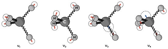
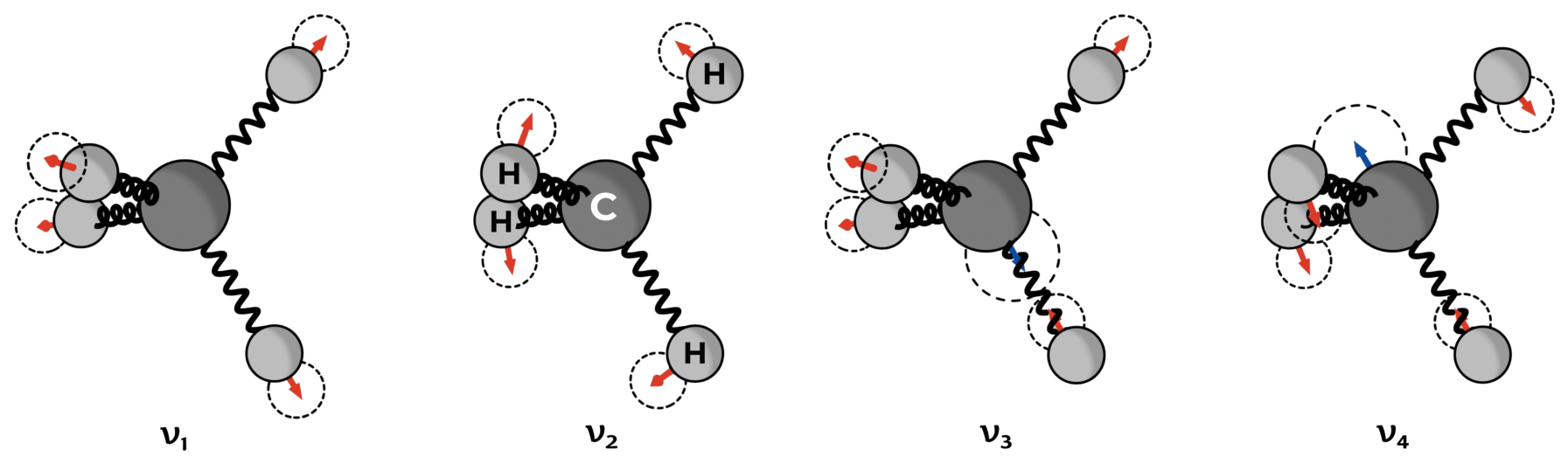
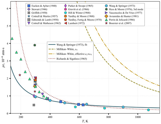
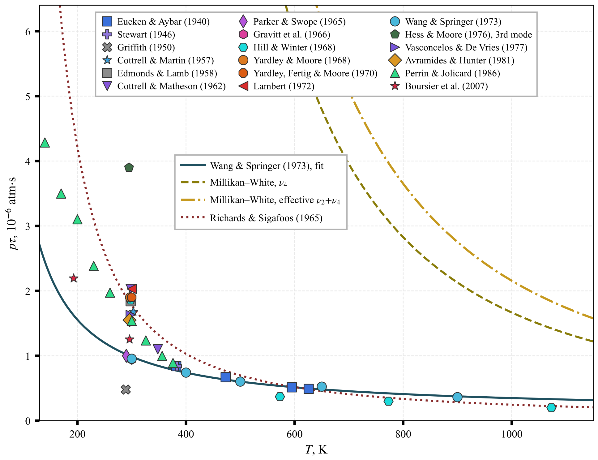
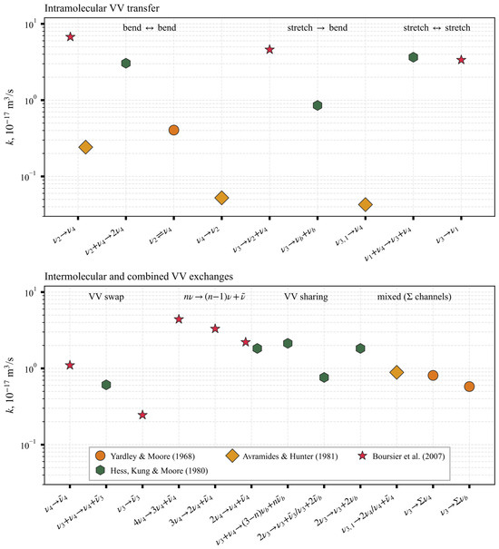
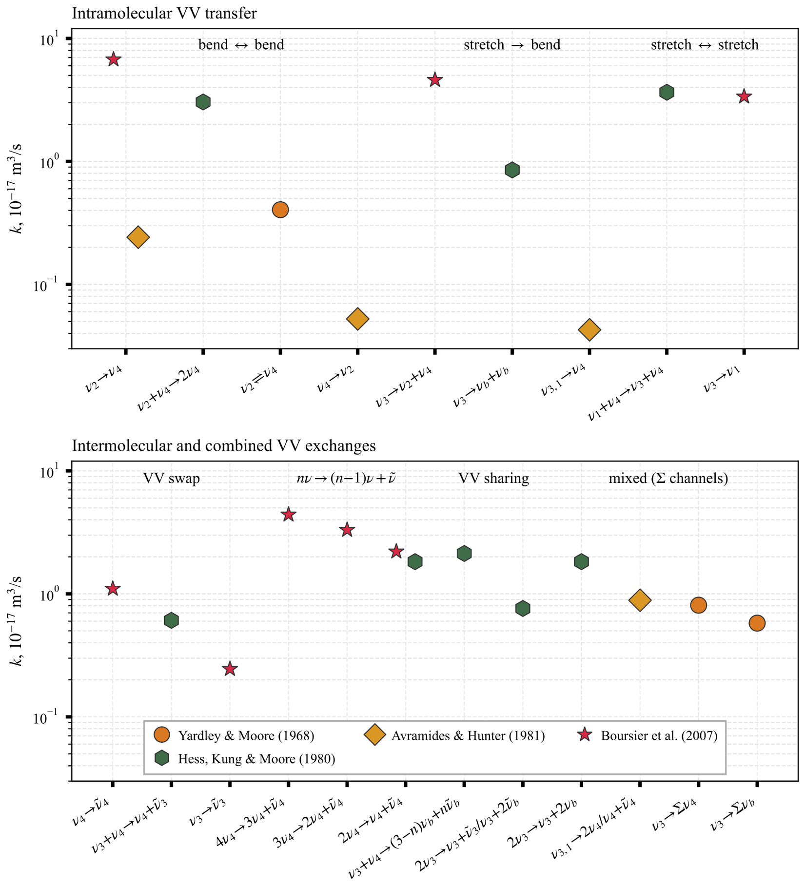
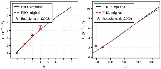
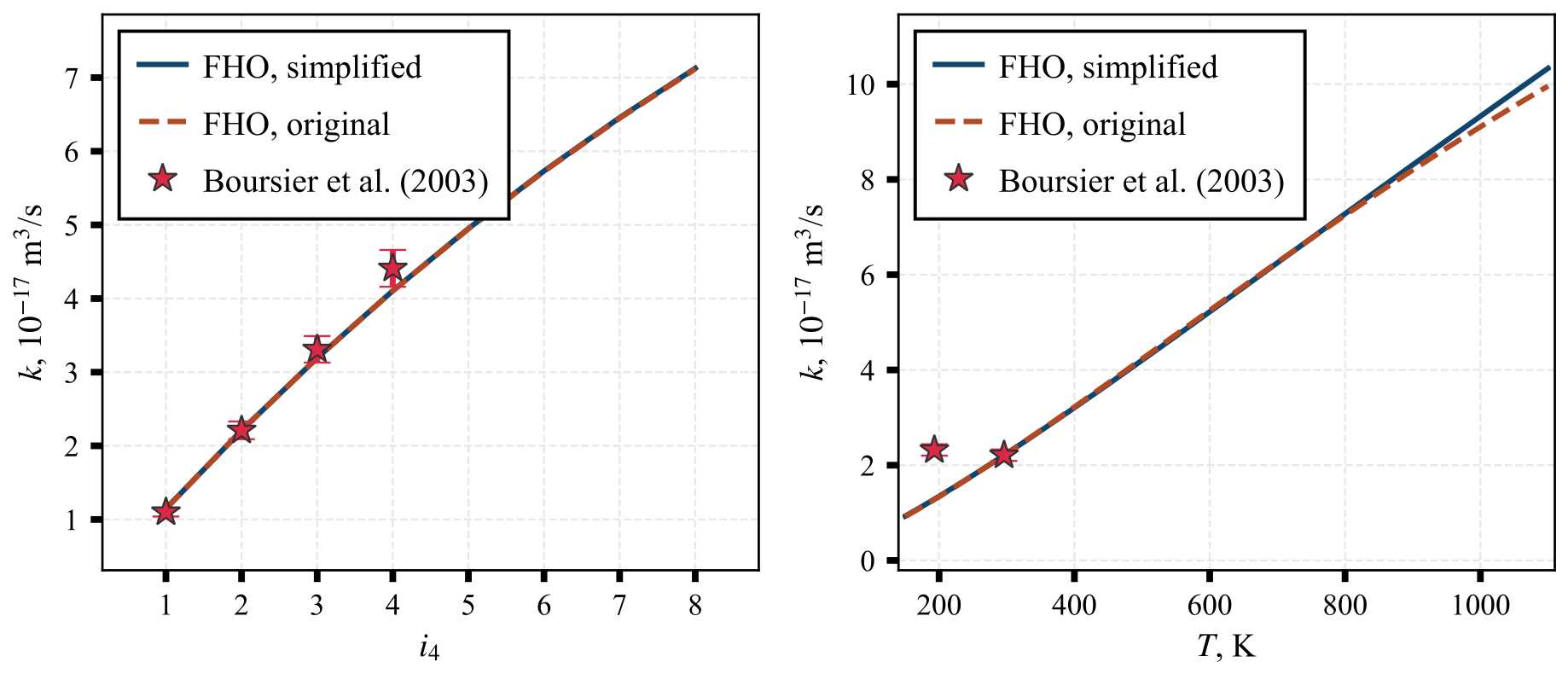
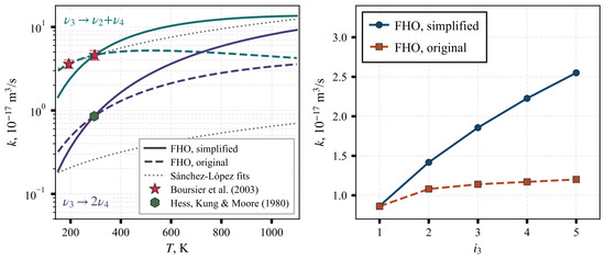
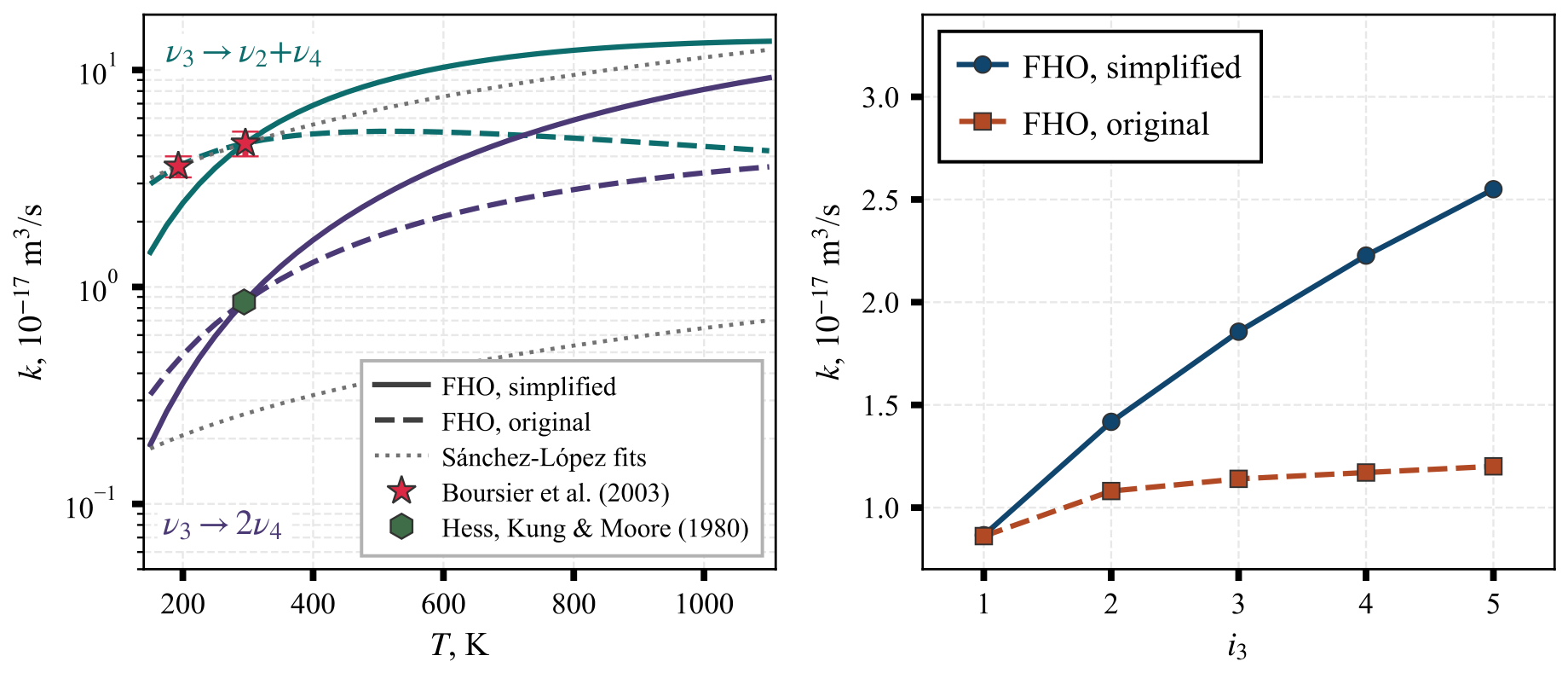
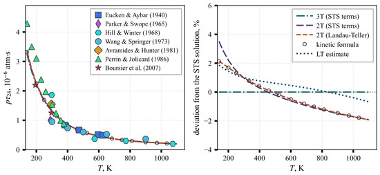
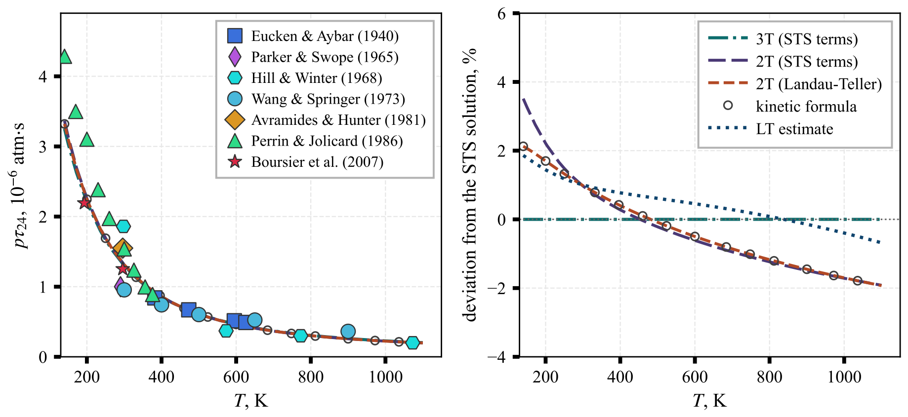
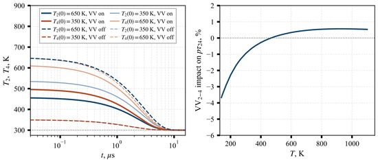
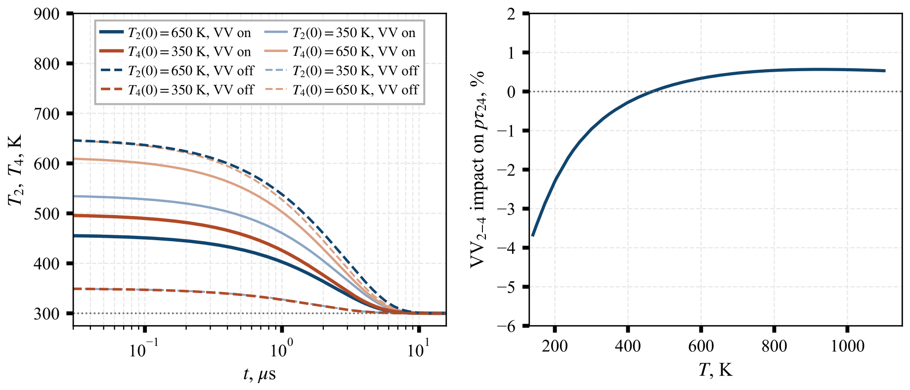
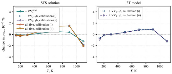
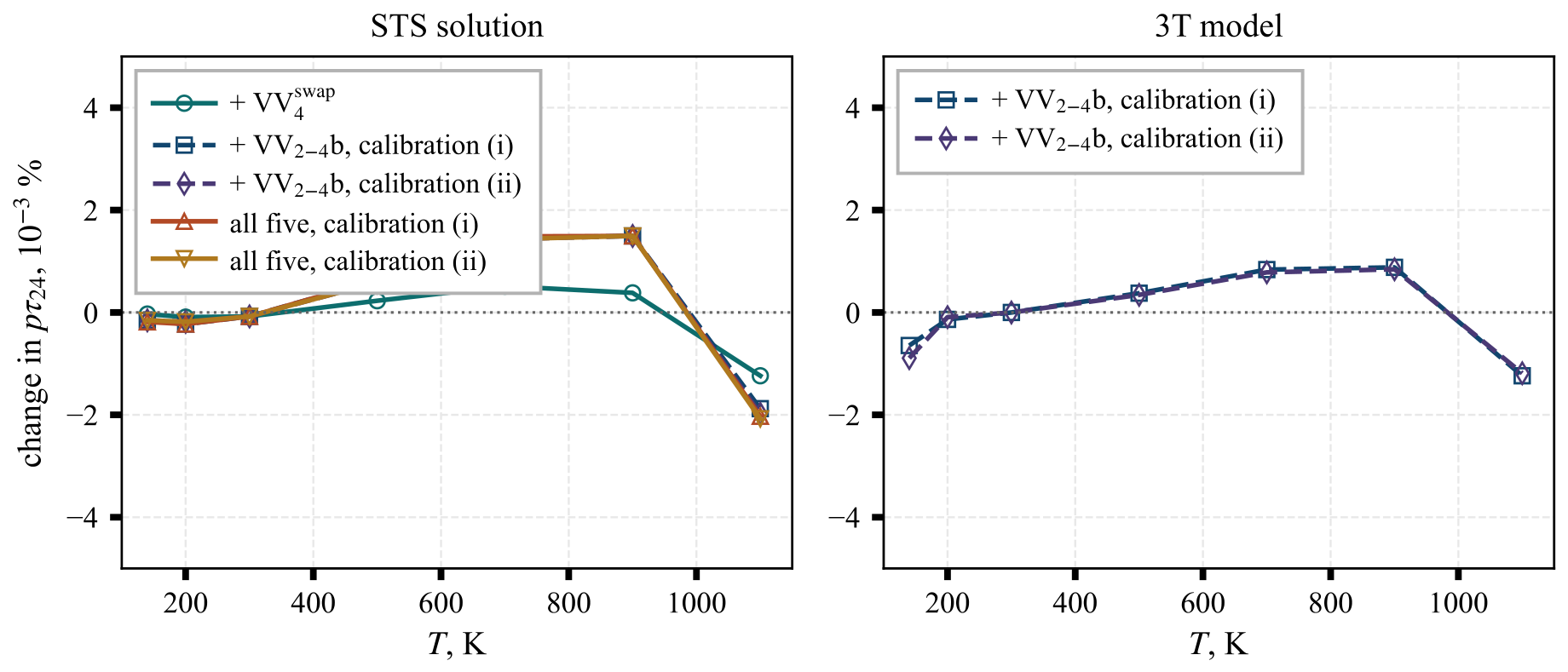
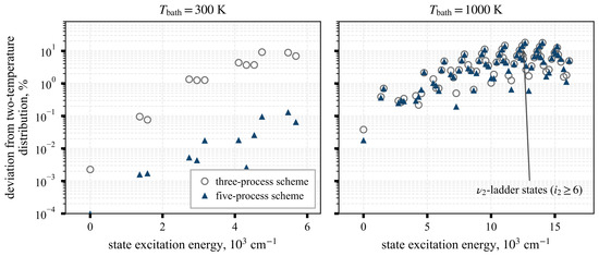
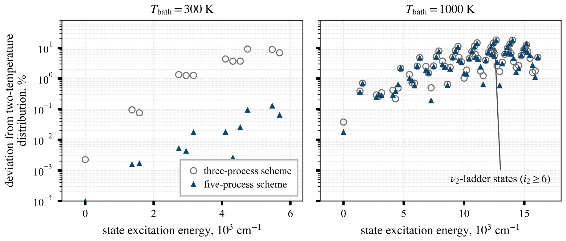
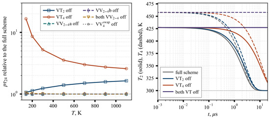
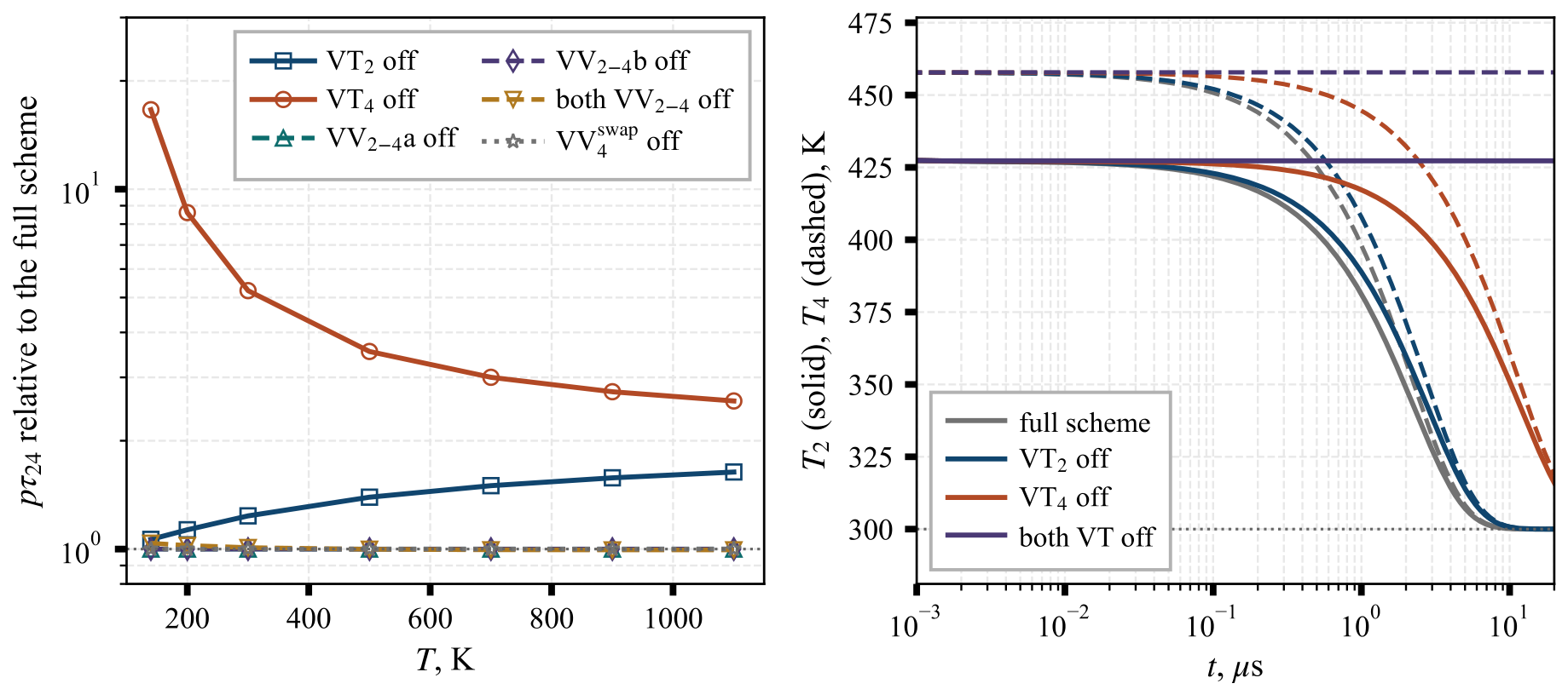

Disclaimer/Publisher’s Note: The statements, opinions and data contained in all publications are solely those of the individual author(s) and contributor(s) and not of MDPI and/or the editor(s). MDPI and/or the editor(s) disclaim responsibility for any injury to people or property resulting from any ideas, methods, instructions or products referred to in the content. |
© 2026 by the authors. Licensee MDPI, Basel, Switzerland. This article is an open access article distributed under the terms and conditions of the Creative Commons Attribution (CC BY) license.