


Abstract
Identifying areas for further wind energy investigation requires information on wind resources, accessibility, and land availability. Yet national screening may select similar areas of land while identifying different locations as assumptions change. This study assesses the geographic persistence of wind energy priorities in Yemen and how alternative electricity network maps affect the interpretation of persistent locations. On a common 1 km grid, wind power density at 100 m and road proximity determine priority, while land exclusions determine fractional availability. Cell recurrence is evaluated across 36 spatial preference analyses and a separate 17-setting weight sweep, with complementary resource formulation and processing diagnostics. Changing the road response function leaves the selected area nearly unchanged but yields a cell set Jaccard similarity of 0.722. Under the reference WPD formulation, their strict intersection retains 14,968 cells covering 12,805.42 km2 (32.9% of reference top 10% area). Alternative resource formulations also change core membership. For these fixed locations, 20.02% of available land lies within 50 km of mapped historical transmission, compared with 68.61% under modeled GridFinder. Governorate patterns and Socotra’s protected area sensitivity reveal differences obscured by national totals. These findings guide resource, land, and electricity infrastructure verification before project-level assessment.
1. Introduction
Renewable energy can help diversify electricity supply and improve energy access, particularly in power systems affected by fuel shortages and infrastructure disruptions [1,2,3]. Wind energy is one option within this transition, but its development potential depends on the spatial distribution of wind resources and the availability of suitable land [4,5]. National wind energy screening therefore helps identify areas that warrant further investigation before detailed wind measurements, land surveys, and electrical infrastructure assessments are undertaken. Geographic information system (GIS)-based multicriteria methods are widely used for this purpose because wind resource conditions must be considered alongside terrain, land use, environmental restrictions, and accessibility [6,7]. These methods have been applied to regional suitability and hybrid wind–solar assessments [8,9], national wind farm site selection [10,11], land evaluation under planning restrictions [12], technical generation potential estimation [13], and geospatial suitability validation [14].
The amount of land assigned to a national priority band and the locations comprising that band are different outcomes. Where selection is defined as a fraction of available land, total area is constrained largely by the rule itself; changes in resource scoring or accessibility preferences can nevertheless replace many of the selected cells. A meaningful robustness assessment must therefore examine not only how much land is selected but whether the same geography remains selected when assumptions change.
This distinction relates to a broader challenge in spatial multicriteria analysis: the dependence of evaluation results on uncertain inputs, criterion weights, and model structure. Previous studies have investigated these sources of uncertainty and their effects on spatial decisions [15,16,17]. Stochastic multicriteria acceptability analysis (SMAA) provides one approach to handling uncertain preferences [18]. It has been incorporated alongside ELimination Et Choix Traduisant la REalité (ELECTRE) methods in wind site assessment [19] and combined with VIKOR (Multicriteria Optimization and Compromise Solution) in renewable energy scheduling [20].
Geographic agreement has also been examined directly in wind siting research. Uguz et al. [21] compared high-suitability cell sets under criterion weight perturbations, while Luukkonen et al. [22] examined spatial overlap between allocations based on biodiversity and distance from settlements across different electricity production scenarios. These studies illustrate the importance of considering geographic agreement alongside other robustness measures. For national screening, cell-level membership within a defined priority band provides a complementary basis for evaluating the geographic consistency of screening results.
The representation of wind resources and land restrictions introduces further variation into this assessment. Large-scale wind energy studies have demonstrated the importance of resource estimation methods, spatial resolution, and land use constraints in determining wind energy opportunities [4,5,23]. Evidence from marine protected area databases shows that gaps in regulatory spatial information can complicate the representation of restricted activities and areas [24]. In addition, wind resource estimates depend on the modeling approaches used to generate them. For example, Liu et al. [25] examined alternative atmospheric modeling configurations, vegetation inputs, and data assimilation procedures against wind observations, illustrating the importance of source model choices and validation. Wind resource representation influences priority, whereas land restrictions determine availability. Keeping these functions separate identifies whether membership changes arise from ordering, available land, or both.
Electricity infrastructure adds another consideration because the usefulness of a candidate area also depends on its relationship to the power system. Spatial network information is widely used in energy system modeling [26], but electricity network datasets may differ in geographic coverage, source records, asset representation, and inferred geometry [27,28,29]. The importance of uncertain inputs and model formulation is also recognized in electricity system planning [30]. Network proximity has been incorporated into wind site suitability assessments [13,14], while regional energy supply datasets provide additional context for relating renewable resources to infrastructure [31]. However, a candidate location can appear relatively close to one mapped network and considerably farther from another without any change in its geographic position or wind resource characteristics. Comparing alternative network representations over the same selected locations therefore helps distinguish changes in mapped infrastructure context from changes in the selection of candidate areas.
These issues are particularly relevant in countries where electricity infrastructure and spatial information are constrained. Yemen provides a suitable national case study because its electricity sector has experienced prolonged disruption since 2015 associated with conflict, fuel shortages, and infrastructure deterioration [1,2,32]. According to the International Renewable Energy Agency, Yemen had approximately 456 MW of installed renewable electricity capacity at the end of 2025, almost entirely solar, with no reported installed wind capacity [33]. Previous studies have also documented challenges involving infrastructure resilience, electricity access, and the transition toward renewable energy [3,34,35]. Under these conditions, national wind energy screening can help organize subsequent investigations, provided that the selected areas are interpreted in relation to the limitations of the underlying resource, land, accessibility, and infrastructure information.
Existing wind energy research provides an important foundation for such investigations in Yemen. Local studies have assessed wind resource characteristics in Ta’izz and Al-Mokha [36,37], Al Hudaydah and Al-Mukalla [38,39], and Socotra [40], while other work has examined local technical and economic feasibility [41]. Broader investigations have addressed national wind resource conditions under present and future climates [42], regional wind climatology [43], and the feasibility of wind energy applications for water supply systems in a United Nations Children’s Fund (UNICEF) study [44]. These studies establish the resource and application context for assessing the geographic stability of national screening results.
While previous wind siting studies, including Uguz et al. [21] and Luukkonen et al. [22], have examined geographic overlap under alternative weights or spatial allocation objectives, the present study links cell-level persistence within cumulative available area priority bands to a fixed-geography comparison of alternative electricity network representations. This distinction allows changes in selected locations to be examined separately from changes in their mapped electrical context.
This study aims to assess the geographic persistence of national wind energy priorities and the dependence of their mapped electrical context on network representation. Using Yemen as a case study on a common 1 km grid, it distinguishes resource–road priority, fractional land availability, persistence under specified spatial and preference changes, and post-selection network proximity. The resulting evidence supports the identification of candidate areas and their requirements for further resource, land, and infrastructure assessment.
The study makes four connected contributions:
- (i)
- A national screening sequence that links resource–road priority, fractional land availability, cell persistence, and post-selection network context.
- (ii)
- A cell-level assessment of persistence across two specified experiments, supplemented by diagnostics of resource formulation, processing, and road reach.
- (iii)
- A comparison of electricity network representations using identical persistent cells and available area weights.
- (iv)
- National and governorate-level evidence linking the screening findings to resource, land, and infrastructure verification needs in Yemen.
The guiding hypothesis is that similar priority band areas can conceal substantial changes in selected cell membership and that persistent locations can have different mapped electrical contexts under alternative network representations.
Three research questions (RQs) guide the investigation:
- (i)
- RQ1. How do wind resource representation and road access preferences shape national priority geography when land availability is accounted for separately?
- (ii)
- RQ2. Which cells remain selected across both persistence experiments under the reference WPD formulation, and how does their persistence change under alternative resource formulations?
- (iii)
- RQ3. How does electricity network representation alter the proximity-based interpretation of fixed persistent locations and the evidence needed for subsequent investigation?
Section 2 reviews the related literature and compares the methodological choices and outputs of recent studies. Section 3 defines the spatial support, priority formation, land accounting, persistence tests, and network comparison. Section 4 reports the results and their implications; Section 5 presents the conclusions.
2. Related Work
Wind energy siting studies commonly combine resource, access, land restrictions, and environmental conditions in GIS-based multicriteria assessment [6,7], although the roles assigned to these inputs differ. Atici et al. [19] excluded ineligible land before ranking or sorting 2 km cells and 13 fields through ELECTRE and SMAA; transmission line distance served as both an exclusion constraint and a weighted evaluation criterion. At the national scale, Atalla et al. [45] used a 26-criterion fuzzy assessment for Kuwait. Analyses by Salih et al. [46], Abdi et al. [10], and Talabă et al. [12] further illustrate differences in how resource, access, and land factors are treated. Excluding unavailable land, scoring eligible cells, and examining uncertain preferences address different questions within these workflows.
For predefined alternatives, a different robustness question concerns how rankings respond to the choice of decision method. Karczmarczyk et al. [17] assessed robustness for seven offshore wind farm projects. Triantafyllidou and Vagiona [47] compared 24 weighting–ranking combinations for 11 eligible areas on Skyros, following spatial restrictions and a minimum feasible site area requirement. Vagiona [48] evaluated 58 existing wind farms using 36 model configurations and a Borda consensus ranking. At the national scale, Aghapour et al. [49] used uniform manifold approximation and projection (UMAP) and K-Means++ to group 55 Iranian regions into 12 clusters and applied several multicriteria decision making (MCDM) methods with consensus aggregation; clustering stability was assessed with the adjusted Rand index. These studies establish how the relative evaluation of predefined areas, farms, or groups varies across models; that evidence is not the same as testing which individual cells enter an area-defined national priority band.
Geographic agreement, rather than ranking agreement alone, has also become a direct object of analysis. Ligmann-Zielinska and Jankowski [16] mapped sensitivity and uncertainty associated with criterion weight variation. In wind energy siting, Uguz et al. [21] compared high-suitability cell sets defined by score quantiles under individual ±10% weight perturbations using Jaccard similarity and separately assessed agreement between candidate zone rankings. Luukkonen et al. [22] selected spatial clusters against capacity-linked land requirements, compared biodiversity- and settlement-oriented allocations, and tested geographic overlap and weight sensitivity. Unlike these approaches, the present study accumulates selected cells by their available land area to define a national priority band. The resulting selection measures are not directly interchangeable across studies. These comparisons show that stable rankings need not imply stable selected geography; spatial agreement must be interpreted in relation to the selection rule and the spatial unit actually tested.
Beyond the choice of weights, wind resource representation can change which places qualify as candidates, whereas electricity network representation changes how an already selected geography is interpreted. Electricity network data may be used as exclusion constraints and/or weighted siting criteria, as in Atici et al. [19], or as inputs to both restriction and suitability, as in Luukkonen et al. [22]. Studies of energy system models, transmission datasets, planning uncertainty, and supply region mapping illustrate the differing purposes and limits of spatial and structural evidence [26,27,28,29,30,31]. Consequently, proximity to a mapped network and the reliability of that mapping should not be confused with verified connection feasibility.
For Yemen, two recent national studies provide complementary evidence on wind resources and site suitability assessment. Gadain and Libanda [42] examined spatial wind resource conditions using the fifth-generation European Centre for Medium-Range Weather Forecasts reanalysis (ERA5), hub height modeling, and Coordinated Regional Climate Downscaling Experiment (CORDEX) projections, addressing the distribution and potential evolution of the wind resource rather than the stability of locations selected by a siting rule. Algawbery et al. [50] developed a seven-criterion GIS–Delphi–full consistency method (FUCOM) suitability assessment and compared its criterion weighting results with the analytic hierarchy process (AHP) and best–worst method (BWM), producing national suitability classes and evaluating weighting consistency and sensitivity. The present study complements this evidence by examining cell-level persistence within national available area priority bands and comparing mapped electricity networks over the same retained locations.
Table 1 compares the spatial units, selection rules, robustness evidence, and network treatment of eight representative studies. The ERA5/CORDEX study is discussed above as resource characterization rather than multicriteria siting.
Table 1.
Methodological comparison of representative wind energy siting and spatial robustness studies.
3. Materials and Methods
Figure 1 establishes the common geography for the analysis, while Figure 2 traces the analytical sequence from independent resource–road priority and fractional land availability to cumulative national priority bands. Within the common 1 km grid, two top 10% recurrence experiments define the strict joint core. Holding that geography fixed enables a network map comparison without site reselection, while complementary road reach and resource form diagnostics qualify its interpretation. Governorate profiles then connect these outputs to evidence needed for further investigation.
Figure 1.
National analytical domain and governorate context of Yemen; numerals identify small or spatially crowded units listed in the map key.
Figure 2.
Analytical workflow separating core-forming persistence analyses, complementary diagnostics, and the fixed location network comparison.
3.1. Study Area and Workflow Overview
Yemen, including Socotra, was represented on a common 1 km × 1 km grid in a Yemen-centered Albers equal area conic projection (origin 15° N; standard parallels 12° and 18° N; central meridian 48° E). Intersection with the adopted land support produced 455,853 represented land cells covering 452,872.58 km2 (Figure 1). This support provides a consistent basis for cell-level comparison and regional aggregation.
Fractional land support is retained in coastal and boundary cells, so the analytical domain area refers to the adopted geometry rather than an alternative official national area estimate. The 1 km grid supports national screening; parcel assessment and micro-siting require finer evidence [23]. The administrative boundaries were obtained from geoBoundaries [51]. The 2017 first-level administrative division (ADM1) layer adopted here contains 22 reporting units, with Amanat Al Asimah (YE-SA) and Sana’a Governorate (YE-SN) treated separately. Cells are assigned to the polygon containing their center or otherwise to the polygon with the largest land area intersection. These assignments remain fixed across analyses. Common cell identifiers connect the inputs and outputs; ADM1 boundaries are used for reporting, while scoring, exclusions, and area calculations remain cell-based.
3.2. Spatial Data and Harmonization
Global Wind Atlas (GWA) version 4 (GWA4) mean WPD at 100 m supplies the reference resource criterion; mean wind speed and International Electrotechnical Commission (IEC) classes I, II, and III capacity factor (CF) layers at the same nominal height supply alternative representations [52,53,54] (Table 2). Road data are restricted to motorway through tertiary classes in the 10 July 2026 Geofabrik OpenStreetMap (OSM) extract [55]. Elevation and Horn slope use the CGIAR Consortium for Spatial Information (CGIAR-CSI) Shuttle Radar Topography Mission (SRTM) v4.1 [56], land cover uses European Space Agency (ESA) WorldCover 2021 v200 [57], and protected areas use the July 2026 Protected Planet extract [58]. United Nations Educational, Scientific, and Cultural Organization (UNESCO) property documentation informs the Socotra representation test [59], and OurAirports supplies locations for the airport buffer cases [60]. GWA4 describes its wind resource mapping at a nominal horizontal spacing of 250 m [52]; the 100 m designation is the resource height, not the horizontal resolution.
Table 2.
Principal spatial datasets and their analytical roles.
Mean WPD, mean wind speed, and the three IEC class capacity factor rasters were separately area-averaged from their source grids to the common 1 km Albers grid and matched by cell identifier. Nearest-road distance was measured from each cell center. SRTM tiles were bilinearly reprojected to a 90 m Yemen Albers working grid, and slopes were calculated in degrees using a 3 × 3 Horn operator. Land-clipped polygon masks exceeding 15°, 20°, and 25° were aggregated as fractional cell exclusions. The adopted protected area extract contained 18 distinct site identifier (SITE_ID) features, including three recorded as Proposed; all were reprojected, repaired where necessary, clipped to Yemen land, and unioned without further attribute filtering during support construction. Land cover support was also intersected with represented land, and overlapping exclusions were unioned before area calculation. Common identifiers support membership comparisons; scenario-specific fractions determine selected area, and baseline (BASE) fractions weight the fixed core network comparison. The 1 km analysis grid is coarser than GWA4’s nominal 250 m mapping; harmonization enables consistent spatial comparisons, but neither increases the atlas’s native wind resource accuracy nor validates site-scale conditions.
Two electricity network representations were compared after selection: the documented World Bank/ENERGYDATA.INFO transmission layer, released in 2017 with a source end date of 2016 [61], and the modeled/predicted GridFinder transmission and distribution layer [29,62]. Neither enters the priority score . Their differing periods and mapped asset types are evaluated separately from priority .
3.3. Resource–Road Priority (Step 2A)
Step 2A in Figure 2 assigns each cell a dimensionless priority score from two explicit screening preferences: mean wind power density at 100 m (W m−2) and proximity to mapped roads, each transformed to a zero to one scale. The score ranks cells, whereas Step 2B determines their available area contributions independently. Electricity network proximity is assessed after selection, and the resource–road score is neither an empirically elicited stakeholder utility nor an estimate of turbine-specific generation.
For cell , let denote mean wind power density at 100 m, area-averaged to the 1 km grid. To bound the effect of extreme values without imposing a wind speed cut-in or saturation threshold, the reference factor is defined by Equation (1), with lower and upper percentile anchors = 27.320734 W m−2 and = 951.255466 W m−2.
The anchors are the 1st and 99.5th percentiles of WPD over all 455,853 represented land cells. They were calculated before exclusions and held fixed across the nine spatial cases, four crossed weight pairs, and 17-point sweep. This clipped linear scale preserves WPD spacing over most of the national distribution while limiting the leverage of upper-tail values. Its bounds are data-dependent preference parameters rather than turbine thresholds. Section 3.9.2 evaluates alternative normalizations and turbine class proxies; the reference road response formulation is retained.
Road accessibility uses the nearest-road distance , measured in kilometers. The reference road response factor in Equation (2) decreases linearly with distance and reaches zero at km:
An alternative road response factor was included in the nine-case spatial robustness design. Equation (3) uses the same road distance field and the same 25 km outer limit but introduces a 5 km breakpoint; distances in Equation (3) are expressed in kilometers:
Road accessibility has been used as a siting criterion in earlier GIS-based wind assessments [50,63,64]. In this study, both road transformations use the same road distance field and assign lower accessibility scores at greater distances. The 25 km limit is a screening parameter tested against and 50 km in Section 3.9.1. Introducing a 5 km breakpoint assigns lower accessibility scores at intermediate distances, testing one direction of response shape change. Project-stage logistics require separate evidence on route geometry, turning radii, turbine component dimensions, pavement and bridge capacity, gradients, local access, and construction conditions.
For cell in analysis , the combined dimensionless priority score is
In Equation (4), and are the power density and road weights, respectively, and is the road response factor for that spatial case. The four exact resource/road pairs in the 36-analysis design are 1/2–1/2, 2/3–1/3, 7/10–3/10, and 11/14–3/14; their decimal labels are 0.500/0.500, 0.667/0.333, 0.700/0.300, and 0.786/0.214. Calculations used the exact fractions, not rounded display values. The reference pair is 0.70/0.30, representing an explicit preference setting after normalization; it is not an empirically measured allocation of explanatory importance. Section 3.7 examines a denser preference range.
Under the 0.70/0.30 reference weights, a 100 W m−2 increase in WPD offsets approximately 6.31 km of additional road distance within the unclipped portions of both factors (Supplementary Section S3). This equivalence expresses the numerical trade-off implied by the scoring rules, not a measured stakeholder preference or an economic optimum. The four crossed preference pairs and the separate 17-point sweep over resource weights of 0.50–0.90 evaluate the spatial consequences of this choice (Section 3.6 and Section 3.7) without calibrating an optimal weight.
3.4. Fractional Land Availability (Step 2B)
Land availability was calculated independently of . Let denote the represented land geometry within cell , and let denote the geometric union of exclusions applicable in analysis . The available fraction was
and the available area contributed by the cell was
where . All areas are expressed in km2; the available fraction is dimensionless.
The baseline exclusion union comprised a slope greater than 15°, ESA WorldCover classes 50 (built-up), 80 (permanent water bodies), 90 (herbaceous wetland), and 95 (mangroves), together with the adopted protected area geometry. The exclusion components were unioned before intersection with the analytical grid.
Fractional accounting retains partial availability within 1 km cells. A high- cell may contribute little land because of exclusions, whereas a largely available cell may rank lower because of weaker resource or access scores. Thus, score order and available area contribution have distinct roles in selection.
3.5. Cumulative National Priority Bands (Step 3)
Within each analysis, cells with positive available area and finite priority scores were ordered nationally by decreasing and accumulated by available area to define cumulative top 5%, top 10%, and diagnostic top 20% bands. All cells tied at a threshold score were retained, so an inclusive band can exceed its nominal percentage when the threshold intersects a large tie block. Top 10% therefore contains top 5%, and top 20% contains both narrower bands.
For cumulative band in analysis , let be the score at which cumulative available area first reaches the nominal target. Inclusive membership was defined as
for cells with , where is the indicator function, equal to one when its condition holds and zero otherwise. The inclusive national band area was
Inclusive membership retains complete equal-score groups and avoids arbitrary ordering within ties. Top 10% serves as an intermediate comparative target, with top 5% and top 20% providing narrower and broader envelopes. Nominal and realized areas are both reported when ties expand selection. Membership uses float64 stored scores with exact strict ( > ), tie ( = ), and inclusive ( ≥ ) comparisons without random tie-breaking or rounding tolerance. The same convention governs all core-forming and road response analyses; only theoretical = 10 km factor endpoints within 1 × 10⁻¹² were canonicalized before score formation.
For governorate ,
where is the governorate priority band area, is the total available area in the governorate, is internal concentration, and is national contribution. Both fractions are dimensionless and reported as percentages. Internal concentration measures the share of a governorate’s own available land that lies within the national band; national contribution measures the share of the national band supplied by that governorate.
3.6. Spatial Preference Persistence: 36 Analyses (Step 4A)
Previous spatial multicriteria research has examined the sensitivity of mapped outcomes to criteria and weight uncertainty [15,16,65]. In the present study, nine spatial cases were crossed with four exact resource/road preference pairs to produce 36 analyses. Each alternative changes a specified BASE component while retaining the reference resource normalization. This deterministic design does not sample a probability distribution or attribute output variance to uncertain inputs and their interactions, as variance-based global sensitivity analysis would require.
BASE combines the linear road response, a 15° slope exclusion, selected WorldCover classes, and the adopted protected areas, with no airport buffer. Eight alternatives comprise slopes of 20° and 25°, the piecewise road response, the Socotra protected area/World Heritage Site (PA-WHS) representation, and four airport buffer configurations (Table 3). All nine cases enter the 36-analysis ensemble. PA-WHS substitutes the terrestrial portion of Protected Planet site 903138 on Socotra as a proxy for the UNESCO terrestrial core [58,59], leaving the mainland unchanged and excluding the UNESCO buffer. This proxy does not replace detailed conservation zoning; airport buffers likewise represent analytical sensitivity parameters. The individual facilities, coordinates, and nested set membership used in the airport buffer tests are listed in Supplementary Table S24.
Table 3.
Spatial cases used in the 36-analysis robustness design.
For cell , top 10% persistence across the 36 analyses was
The count records the number of 36 analyses in which cell belongs to the inclusive national top 10% band. A count of 36 indicates full recurrence across the specified cases; lower counts show dependence on tested spatial settings and weights. This deterministic recurrence is not a statistical confidence level.
3.7. Preference Weight Persistence: 17-Setting Sweep (Step 4B)
A separate 17-point sweep evaluates BASE resource weights from 0.50 to 0.90 in increments of 0.025, providing finer coverage than the four crossed pairs. This is a declared sensitivity range rather than an elicited probability distribution of preferences. The resource weight at point is
with
The inclusive national top 10% band was reconstructed at each weight using the same resource scale, road data, BASE availability, and tie convention. Recurrence, governorate rank and contribution ranges, and Jaccard overlap summarize the response. Cells selected at all 17 discrete weights form the preference-persistent set.
For two nonempty membership sets and , the Jaccard overlap J(A,B) was
3.8. Strict Joint Persistent Core (Step 5)
Let contain the cells present in the inclusive top 10% band in every one of the 36 spatial/preference analyses, and let contain those selected under all 17 preference weights. Their strictly persistent joint core is defined by Equation (14). The same definition is independently applied to each tested resource formulation; no cross-formulation intersection is substituted for its reference-specific joint core.
In Equation (13), vertical bars denote the number of cells in a set. Jaccard overlap describes set agreement by cell count; geographical areas are calculated using the fractional available-area weights, not nominal 1 km2 cells. Complementary road distance and resource model diagnostics do not enter the definition of the joint core. An additional 90% recurrence diagnostic requires membership in at least 33 of the 36 scenarios and at least 16 of the 17 sweep cases; it is a deterministic relaxation of the intersection rule, not a confidence interval or selection probability.
Core area is calculated by summing BASE available area weights over persistent cell identifiers, regardless of the spatial case in which selection occurred. It therefore represents BASE-available land at persistent locations rather than the geometric intersection of scenario-specific available polygons. The network comparison holds both identifiers and weights fixed. Resource score comparisons use the same area accounting convention.
3.9. Complementary Sensitivity Diagnostics
The reference core intersection tests recurrence under its declared spatial and preference conditions. Road reach and resource formulation diagnostics test further sources of geographic sensitivity without changing that core definition.
3.9.1. Road Reach Sensitivity
Road reach sensitivity is evaluated with linear road response scales , 25 and 50 km (D10, D25 and D50), retaining the 0.70/0.30 reference preference, resource representation, and BASE availability. This diagnostic varies the reach of accessibility scoring separately from the response shape alternative included among the nine spatial cases.
For each distance scale, inclusive top 10% membership, selected area, pairwise Jaccard overlap, and governorate contribution and rank were calculated. The intersection across the three scales measures road reach persistence separately from the joint core defined by the 36-analysis ensemble and the 17-weight sweep.
Selection retains boundary ties at each scale, including equal composite scores produced by flat accessibility segments. Selected area and membership are therefore calculated from each inclusive threshold rather than inferred from the nominal 10% target.
3.9.2. Wind Resource Formulation and Processing Sensitivity
Resource formulation was varied independently of the spatial and preference settings. The reference WPD scale uses the all-land 1st and 99.5th percentiles (P01–P99.5); alternatives use bounded 5th–99th percentile scaling (P05–P99), full-range Min–Max scaling, and empirical percentile rank. Defining each transformation over all represented land cells and holding it fixed as availability changes prevents exclusions from altering the resource score definition.
Resource model sensitivity was evaluated using four wind power density normalizations, IEC I, II, and III capacity factor layers under four scoring transformations each, and an auxiliary piecewise-linear mean wind speed proxy. For the capacity factor layers, the four transformations were the native fractional values, full-range Min–Max, bounded 5th–99th percentile scaling, and empirical percentile rank.
The auxiliary wind speed score W57 is zero at or below 5 m s−1, increases linearly to one at 7 m s−1, and remains one above that value. Two auxiliary anchor variants, W56 (5–6 m s−1) and W58 (5–8 m s−1), are used only for the saturation comparison reported in Supplementary Table S18; they are not additional members of the 17 resource score specifications. These anchors are screening score parameters, not turbine cut-in or rated speed thresholds. Distinct from the 17 preference weight settings in Section 3.7, these 17 resource score specifications comprise four WPD normalizations, twelve IEC-based variants, and W57. The capacity factor layers describe representative turbine class performance under their source model assumptions, not observed site-specific annual generation.
The published GWA methodology describes representative gross capacity factor calculations at 100 m using IEC-class turbine power curves [53]. Because that account predates GWA4, its specific turbine models and curves are not attributed to the Yemen CF rasters without source release confirmation; the present comparisons retain their role as model-based screening proxies. The IEC-CF proxies are distinct from the separate IEC turbine siting classification layers derived from the Global Atlas for Siting Parameters (GASP) project [66].
Each of the 17 resource specifications was evaluated using the same nine spatial cases, four preference pairs, and 17-point sweep, with common cell identifiers, area accounting, and inclusive tie rules. Comparisons quantify top 10% membership, pairwise Jaccard overlap, recurrence within each design, and their joint intersection. Upper clipping is the fraction of selected available area assigned the maximum resource score. Because normalization changes score spacing and its balance with road proximity, differences in core size and overlap are interpreted as formulation sensitivity rather than evidence that one scale predicts wind production more accurately.
Processing sensitivity was assessed by resampling the native GWA WPD raster to the same 1 km grid using area averaging, bilinear interpolation, and nearest-neighbor interpolation. Area averaging supplied the reference. Each alternative used its own national and score anchors, with road distance, the 0.70/0.30 preference, available area weights, cell identifiers, and the inclusive top 10% rule held fixed. Cell set Jaccard and retention of reference-selected available area measure the resulting processing sensitivity. The experiment compares neither independent wind observations nor different source model resolutions.
To examine variation within the common grid, the standard deviation and extrema of native source WPD were calculated for each 1 km cell. Separate sensitivity cases represented each cell by its native source minimum or maximum rather than its area-averaged mean while retaining the original WPD normalization bounds, road scores, BASE availability, and inclusive selection rule. These cases compare alternative cell-level representations of the same modeled source, not site selection on the native raster with finer land exclusions. Within-cell dispersion was evaluated from the warped first and second WPD moments as the square root of their nonnegative variance; minimum and maximum representatives were derived by the corresponding raster resampling operations. The source to cell summaries use the same 1 km support and do not recalculate subcell slope exclusions or road distances.
Input sensitivity was also examined by multiplying the reference WPD field uniformly by 0.80, 0.90, 1.10, and 1.20 before applying the original 27.320734–951.255466 W m−2 normalization bounds. The unperturbed case was checked against BASE, and each alternative was reranked using the same roads, available area weights, and top 10% rule. These deterministic shifts are illustrative stresses on the modeled input, not estimated error bounds for Yemen. The symmetric 10% and 20% magnitudes were chosen as two transparent hypothetical stress levels in each direction rather than inferred from an error distribution or calibrated to the external validation sample.
3.10. Fixed Geography Electricity Network Comparison (Step 6)
Mapped network proximity was evaluated using identical reference core cell identifiers and BASE available area weights. Holding geography and weights fixed isolates differences between the line representations and changes in site selection. Table 4 summarizes their provenance and scope of interpretation.
Table 4.
Infrastructure representations used in the post-screening distance diagnostic.
The Legacy layer describes a documented historical transmission backbone [61], whereas GridFinder combines observed OpenStreetMap lines with inferred transmission and distribution features [29,62]. Their differences in vintage, asset type, coverage, and modeling assumptions make the comparison one of infrastructure representation rather than verified network expansion. GridFinder’s road-weighted prediction of medium voltage routes also creates a potential shared data dependence with the road access factor used in priority formation.
Spearman rank correlations between OSM road distance and nearest mapped line distance were calculated for each network on the fixed BASE top 10% set and its strict core subset. This diagnostic measures association within a selected geography. It cannot establish causal dependence or statistical independence, particularly given the road information used to infer some GridFinder routes [29].
A complementary comparison grouped the fixed strict core cells by their original nearest-road distance (0–5, 5–10, and 10–25 km). Within each group, the shares of BASE-available core area lying within 50 km of Legacy and GridFinder were calculated using the same nearest-line distances, with the BASE-available core area in the respective road distance group as the denominator. This stratification tests whether the mapped network contrast persists within road distance bands; it does not remove the possible shared data dependence of GridFinder and OSM roads.
Nearest mapped line distance was calculated from each selected cell center to the network polylines in the Yemen Albers equal-area projection using planar Euclidean geometry. The identical distance convention was used for the documented transmission layer and GridFinder. Medians summarize cell-level nearest-line distances without area weighting. The proportions within 10, 25, 50, and 100 km and beyond 100 km were computed by summing BASE available area weights over qualifying core cells and dividing by total available core area. Governorate-level proportions use the corresponding governorate core area as the denominator.
The 50 km summary is an intermediate reporting distance; its engineering relevance depends on voltage, plant size, terrain, and system architecture. Additional thresholds expose how representation differences vary with distance. Connection appraisal requires asset condition, voltage, operating status, capacity, impedance, connection cost, and hosting capability. National 33/11-kV statistics provide context, but an equivalent current countrywide distribution network GIS vector was unavailable.
3.11. Spatial Outputs and Interpretation Metrics (Step 7)
Governorate planning profiles combine BASE top 10% area, internal concentration, and national contribution with joint core area and share and mapped network proximity (Section 4.6). Supplementary Table S9 reports preference weight rank ranges and separate road response ranks. The measures are interpreted jointly without combining them into a suitability or investment score.
Governorate ranks describe national top 10% contribution. Best and worst valid ranks summarize the 17-point preference sweep, with 1–1 denoting consistently first; unsupported or undefined ranks are not reported. Road response ranks follow a D10/D25/D50 order with complete boundary ties. If ties expand an inclusive band, its rank comparison is not interpreted as an equal area comparison. Governorates with zero national top 10% contribution remain unranked. These summaries describe available candidate geography, not electricity demand, projected generation, population served, or investment performance.
3.12. Quality Assurance and Reproducibility
Quality checks covered grid alignment and identifiers, represented land and fractional exclusions, score transformations, inclusive area-weighted selection, persistence counts, governorate assignment, and network distance denominators. Membership and area totals were independently cross-checked against cell-level records. All resource specifications and spatial or preference cases used consistent selection and area accounting rules. The within-cell WPD diagnostic retained BASE exclusion fractions and checked reconstructed scores against the reference using the moment and extremum calculations described in Section 3.9.2.
The WPD reference scores and membership were reproduced using the specified source raster, road distance field, fractional BASE availability, and inclusive threshold rule. The geometric grid definition, resource file characteristics, airport facility sets, and resource form consistency checks are described in Supplementary Section S21 (Tables S23 and S24). These checks concern spatial inputs and deterministic selection rather than independent wind measurements or site-level feasibility.
4. Results and Discussion
The results distinguish the amount of land selected from the identity of the selected cells and then examine which locations persist under the declared tests and how their mapped electrical context varies. This progression makes it possible to interpret a stable area total without assuming stable geography or verified grid access. Unless stated otherwise, the resource criterion is the reference WPD score at 100 m.
4.1. Spatial Distribution of Priority and Available Land
The reference 0.70/0.30 resource–road weighting produces a geographically uneven composite priority score across Yemen (Figure 3a). The cumulative bands in panel (c) show where that ordering translates into selected cells after fractional land availability is accounted for. The bounded WPD scale differentiates resource conditions, and road proximity adjusts national ranking; neither map is an estimate of turbine-specific generation.
Figure 3.
BASE screening using the WPD-based resource score and reference resource–road weights (0.70/0.30): (a) composite priority score; (b) available fraction of represented land following land exclusions; (c) non-overlapping segments of the cumulative national top 5%, top 10%, and top 20% bands; and (d) selected available area for the cumulative bands. Colored map cells represent 1 km grid footprints, whereas the selected area totals use the fractional available area of each cell.
The spatial pattern of the BASE priority bands broadly accords with that reported by Algawbery et al. [50], although differences in criteria and output definitions preclude equivalence between their suitability classes and the present priority bands. Land exclusions further differentiate the candidate footprint: 389,440.92 km2 remains available within the 452,872.58 km2 represented domain (86.0%; Figure 3b). Availability is extensive across much of eastern Yemen and more fragmented in the mountainous west, so a high priority score need not imply a large available area.
The cumulative top 5%, top 10%, and top 20% bands contain 19,472.69, 38,944.55, and 77,888.71 km2, respectively (Figure 3c,d). The top 10% band comprises 45,998 cells with unequal available area contributions. Only one cell lies at its threshold, and top 20% also remains close to its nominal target. The band areas consequently follow the cumulative area rule closely; the informative spatial outcome is the identity and distribution of the cells supplying them.
National Contribution Versus Within-Governorate Concentration
A governorate can supply a large share of the national band while having only a small proportion of its own available land selected. National contribution and internal concentration capture these distinct patterns (Table 5; Figure 4). The former measures a governorate’s share of national selected land; the latter describes selection within its own available area.
Table 5.
Selected governorate results for the WPD-based BASE inclusive national top 10% band (resource–road weights 0.70/0.30).
Figure 4.
Governorate distribution of the WPD-based BASE priority bands: (a) share of each governorate’s available land contained in the cumulative national top 5%, top 10%, and top 20%; (b) each governorate’s contribution to the available area of those national bands; and (c) contrast between internal top 10% concentration and national top 10% contribution. Panels (a) and (b) share governorate ordering but have separately labeled percentage scales.
Hadramaut and Al Mahrah dominate the national top 10% band, contributing 14,876.16 km2 (38.20%) and 8500.56 km2 (21.83%), together 60.03%. Yet the band contains only 9.94% and 14.14% of their respective available land. Their dominance therefore reflects extensive candidate geography rather than selection of most locally available land. Their combined contribution changes to 53.22% in the top 5% and 53.21% in the top 20%, showing that the inclusion threshold also affects regional composition.
Ta’izz and Lahij show a more concentrated pattern: their selected areas are smaller, at 3815.84 km2 (9.80% nationally) and 3268.94 km2 (8.39%), but contain 48.79% and 33.33% of locally available land. Shabwah contributes 4095.27 km2 (10.52%) with an internal concentration of 12.73%. These five governorates together supply 88.73% of the national selected area, but their contrasting balances of extent and concentration imply that contribution alone cannot characterize the candidates.
Small available land denominators produce a different contrast. Socotra’s 8.05 km2 selection occupies 97.45% of its 8.26 km2 BASE-available land but contributes only approximately 0.02% nationally. Aden similarly contributes 451.81 km2 (1.16% nationally) while including 69.52% of its own available land. Al Hudaydah and Al Jawf supply larger areas, 829.24 km2 (2.13%) and 682.45 km2 (1.75%), respectively. These differences make both the extent of selected land and its local concentration relevant to interpreting subsequent sensitivity and persistence.
4.2. Land and Accessibility Effects on Selection
Exclusions change the amount and distribution of available land, whereas weighting and road response assumptions change its ordering. Figure 5 compares the resulting changes in selected extent and cell membership.
Figure 5.
Sensitivity of WPD-based top 10% selection: (a) change in selected available area and cell membership Jaccard similarity across nine spatial cases relative to BASE; (b) Jaccard similarity across 17 preference weights relative to 0.70/0.30; and (c) selected available area and Jaccard similarity for road response reaches of 10, 25, and 50 km, relative to 25 km. Airport labels indicate facility counts and buffer radii. Panels (a) and (c) test road response shape and reach, respectively.
4.2.1. Land Restrictions and Available Area Effects
Relaxing the slope threshold expands available land with little change in selected cell identity. Moving from 15° to 20° increases availability from 389,440.92 to 412,974.01 km2 and top 10% area from 38,944.55 to 41,297.84 km2 (6.04%). At 25°, these totals reach 428,212.04 and 42,821.94 km2 (9.96%). The increases follow the enlarged available area denominator under an unchanged WPD score. Other exclusions have smaller national effects: PA-WHS increases availability to 390,288.73 km2 and selected area to 39,029.38 km2 (0.22% above BASE), while the four airport buffer cases yield 38,866.55–38,926.75 km2.
4.2.2. Preference Weights and Road Response Sensitivity
Unlike slope relaxation, changing preference weights or road response shape mainly replaces that cells are selected, rather than changing the total selected area. Over resource weights of 0.50–0.90, the top 10% area remains near its nominal 38,944 km2 target, yet only 21,509 of the reference band’s 45,998 cells occur at all 17 weights (Figure 5b). The alternative road response shape similarly selects 38,944.81 km2, just 0.00066% above BASE, but its cell set Jaccard is 0.722. By comparison, the 20° and 25° slope cases retain Jaccard values of 0.994 and 0.995 despite their larger area increases (Figure 5a). Thus, area expansion under slope relaxation is geographically different from the replacement induced by accessibility preferences. The response shape alternative forms part of the nine-case ensemble; changes in road reach are tested separately.
The road reach comparison reinforces this distinction (Figure 5c). Scales , 25, and 50 km select 46,395, 45,998, and 45,546 cells, contributing 38,944.48, 38,944.55, and 38,944.24 km2, respectively. Relative to D25, Jaccard falls to 0.598 for D10 and 0.710 for D50. Only 27,938 cells are common to all three scales, representing 23,542.00 km2 or 60.45% of the D25 selected area. This road reach intersection quantifies a separate sensitivity dimension from the strict joint core formed by the 36-analysis ensemble and 17-weight sweep.
The geographic replacement apparent at the cell level is partly obscured by governorate-level rankings: regional contributions change with road reach even when the leading governorates remain the same. Hadramaut supplies 31.31%, 38.20%, and 40.36% of the national top 10% area under D10, D25, and D50, while Al Mahrah supplies 15.53%, 21.83%, and 26.81%. Ta’izz and Shabwah exchange third and fourth ranks between D10 and D25. Relatively stable administrative rankings can therefore coexist with substantial changes in the cells selected within them.
4.2.3. Local Effects of Exclusion Data: Socotra
The converse problem arises when the national effect of land exclusion is small but its local effect is substantial. On Socotra, replacing the BASE protected area geometry with PA-WHS increases available land from 8.26 to 856.07 km2, although the national denominator rises by only approximately 0.218%. This contrast explains why the small national PA-WHS response cannot characterize the island’s sensitivity.
With wind and road scores held fixed, the Socotra selection expands from 272 cells contributing 8.05 km2 under BASE to 1473 cells contributing 855.80 km2 under PA-WHS. These areas represent 97.45% and 99.97% of the respective available land totals. The local gain of approximately 847.75 km2 exceeds the national increase of about 84.83 km2, from 38,944.55 to 39,029.38 km2, because the cumulative selection rule redistributes membership nationally. The result identifies conservation area representation as a major local influence on candidate geography. Site-level interpretation requires reconciliation of the PA-WHS proxy with current protected area boundaries and conservation restrictions [58,59].
4.3. Resource Formulation and Spatial Agreement
Wind resource formulation and processing can alter selected cell membership even when land availability is unchanged. The following analyses examine resource scaling, source to grid representation, and uniform WPD perturbations.
4.3.1. Resource Score Formulation and Geographic Overlap
The reference WPD scale is bounded by the national 1st and 99.5th percentiles, 27.32 and 951.26 W m−2, calculated over represented land before exclusions (Figure 6a). These fixed bounds provide a common score scale across spatial cases. They express distribution-based screening preferences rather than turbine operating limits.
Figure 6.
Sensitivity to WPD normalization: (a) resource score transformations; (b) cell membership Jaccard similarity for BASE top 10% selections and strict joint cores relative to P01–P99.5; and (c) available-area-weighted score state proportions within each formulation’s own top 10% band. Panel (a) displays 0–1200 W m−2; full-range Min–Max normalization uses the observed maximum of 9449.91 W m−2. Zero, intermediate, and maximum score states are preference scores, not capacity factors.
Spatial agreement is sensitive to the choice of WPD normalization (Figure 6b). Relative to –, – gives Jaccard values of 0.865 for BASE top 10% membership and 0.811 for the joint core. The corresponding values are 0.235 and 0.177 for full-range Min–Max and 0.800 and 0.575 for the percentile rank. The particularly low Min–Max agreement is consistent with the effect of the unusually high national maximum: scaling to this value compresses differences among most cells and changes the resource factor’s effective balance with road proximity.
Counting persistent cells alone cannot establish whether an alternative formulation retains the same persistent locations. The –, –, full-range Min–Max, and percentile rank scales retain 14,968, 16,572, 22,989, and 23,432 core cells, respectively. Larger recurrent sets under an alternative scale reflect how scores are constructed; they do not establish better resource quality or predictive validity. Supplementary Table S13 reports the selected and core counts and areas for all resource formulations.
The IEC capacity factor comparisons further distinguish similarity in size from agreement in location. Under –, IEC I, II, and III retain similarly sized cores of 17,180, 17,219, and 17,240 cells (Supplementary Table S13). Cell-matched comparisons provide the geographic evidence: across the twelve IEC-CF alternatives, Jaccard relative to the reference WPD formulation ranges from 0.578 to 0.731 for BASE top 10% membership and from 0.446 to 0.676 for strict joint core membership (Supplementary Table S19). The alternatives retain 65.0–76.6% of reference core cells and 69.4–80.9% of its BASE-available area.
Holding normalization fixed reveals closer agreement among the IEC classes: pairwise Jaccard ranges from 0.878 to 0.965 for BASE top 10% membership and from 0.847 to 0.960 for strict cores (Supplementary Table S19). Their greater agreement with one another than with WPD indicates that selected geography depends on resource representation, even under a common scoring rule. These model-based comparisons describe spatial agreement among screening proxies, not independently validated turbine-specific production.
The clipping diagnostics explain a further difference between resource scores (Figure 6c). Under –, the maximum resource score accounts for 1.46% of the formulation’s own BASE top 10% available area compared with 5.41% under –. Full-range Min–Max and percentile rank assign negligible area exactly to the maximum, consistent with their definitions. These fractions describe score scaling, not turbine performance or resource model accuracy.
Saturation is much more extensive in the auxiliary wind speed formulations. Under W57, 33,582 out of 42,143 top 10% cells receive the maximum wind score, representing 79.69% of cells and 80.33% of the selected available area. Under W56, the corresponding figures are 40,986 out of 43,594 cells, 94.02% of cells, and 94.31% of the area (Supplementary Table S18). Unlike normalization alone, the auxiliary wind speed comparison changes both the physical resource indicator and its scaling. These results characterize formulation-dependent discrimination within the selected band without identifying universally preferred normalization.
4.3.2. Spatial Representation of the Source WPD Raster
The representation of the same source raster on the common analytical grid creates a further distinct source of membership change. Relative to area averaging of the same GWA WPD source, bilinear and nearest-neighbor representations yield Jaccard values of 0.955 and 0.822 and retain 98.38% and 92.73% of the reference selected available area. Each selects approximately 38,945 km2. Because each representation recalculates its own percentile anchors, these differences reflect the combined effects of resampling and score normalization. They reveal processing-dependent geographic selection on a fixed analytical grid; they do not demonstrate improved WPD accuracy or estimate independent wind resource error.
Native source variability qualifies this comparison further. Across BASE-available land, the area-weighted mean of within-cell WPD standard deviation is 18.53 W m−2, increasing to 34.04 W m−2 in the reference top 10% band and 39.87 W m−2 in the strict core (Supplementary Table S20). Replacing area-averaged WPD with native source cell minima or maxima leaves selected area near 38,945 km2 but reduces top 10% cell set Jaccard relative to the reference to 0.680 and 0.582, respectively. The resulting geographic replacement measures sensitivity to how modeled WPD is represented within the 1 km grid without estimating wind resource error or repeating land exclusions at native resolution.
4.3.3. Declared Uniform WPD Perturbations
Unlike the changes in resource formulation and source to cell representation, the declared uniform WPD stress produces more limited, though still nonzero, geographic replacement. With the normalization bounds fixed, WPD multipliers of 0.90 and 1.10 yield top 10% Jaccard values of 0.943 and 0.947; multipliers of 0.80 and 1.20 reduce these to 0.881 and 0.901 (Supplementary Table S21). Between 93.9% and 97.3% of the reference selected available area is retained across the four nonreference cases. Uniform scaling changes resource score spacing relative to road proximity and may change clipping at the fixed anchors. It does not reproduce spatially heterogeneous atlas errors or assign statistical confidence to retained locations.
The reference strict core must therefore be interpreted as persistence under the declared WPD scale and its spatial and preference tests. Resource form and processing comparisons define the limits of that interpretation rather than extending the core to all tested representations. For candidate areas where this resource form dependence matters to further investigation, measurement-supported, finer-scale wind modeling is a relevant next step. The locally adjusted Weather Research and Forecasting (WRF) simulations and observational validation reported by Liu et al. [25] in forested terrain illustrate one such approach, not a model validated for Yemen or a substitute for local wind measurements.
4.4. Conditional Persistence of Priority Locations
Under the reference WPD formulation, the intersection of the two full-recurrence sets identifies the locations retained across both persistence experiments (Figure 7). Out of 455,853 represented land cells, 79,534 enter at least one of the 36 spatial preference top 10% bands and 19,938 enter all 36, equivalent to 25.1% of the ever-selected set. Figure 7b displays recurrence within that set, excluding the 376,319 zero-frequency cells. The separate BASE preference sweep retains 21,509 cells at all 17 weights. The first experiment combines exclusion and preference changes, whereas the second samples preferences more densely under fixed BASE conditions.
Figure 7.
Persistence of WPD-based top 10% membership: (a) selection frequency across 36 crossed analyses; (b) frequency distribution among 79,534 cells selected at least once, excluding 376,319 zero-frequency cells; and (c) intersection of the all-36 and all-17 persistent sets defining the strict joint core. Frequencies describe recurrence under the tested scenarios, not statistical probabilities.
Their intersection contains 14,968 cells, and 4970 occur only in the all-36 set and 6541 only in the all-17 set, giving a cell count Jaccard of approximately 0.565 (Figure 7c). Full recurrence in either experiment is therefore insufficient to establish recurrence in both. Weighted by BASE fractional availability, the joint core contains 12,805.42 km2 or 32.9% of the reference top 10% area. This intersection defines the conditional geography used for the subsequent infrastructure comparison.
The recurrence requirement materially affects the retained footprint. A 90% rule requiring at least 33 out of 36 spatial preference memberships and at least 16 out of 17 weight memberships retains 22,925 cells and 19,688.02 km2 of BASE-available land (Supplementary Table S11). Compared with the strict intersection, this deterministic relaxation tolerates limited membership changes within the same test space; it does not assign statistical confidence to the additional locations.
Persistence also shifts the regional balance (Table 6). Hadramaut supplies 3327.83 km2 (25.99%) of the core area, Ta’izz 2673.80 km2 (20.88%), Al Mahrah 2560.09 km2 (19.99%), Lahij 2441.81 km2 (19.07%), and Shabwah 1205.06 km2 (9.41%), together approximately 95.34%.
Table 6.
Selected governorate contribution and retention from the BASE top 10% band to the strict joint persistent core.
Although the eastern governorates remain substantial contributors, Ta’izz and Lahij retain 70.07% and 74.70% of their BASE selected area compared with 22.37% in Hadramaut and 30.12% in Al Mahrah. The large eastern baseline footprint thus differs from the higher local retention observed in the southwest.
4.5. Network Representation and Electrical Context
Cells recurring in both reference persistence experiments provide a geographically defined basis for assessing electricity network context. Holding the 14,968 core cells and their 12,805.42 km2 of BASE-available land fixed reveals how mapped proximity differs across network representations (Figure 8). The share within 50 km is 20.02% under documented historical transmission (Legacy) and 68.61% under GridFinder, a difference of 48.59 percentage points. Both values use identical cell center to line geometry and area weighting, so the contrast arises from the alternative mapped networks rather than site reselection.
Figure 8.
Geographic context of the fixed WPD joint core relative to (a) documented historical transmission (Legacy) and (b) modeled/predicted GridFinder. Shaded 50 km reach is a visualization of mapped geographic distance; the reported within 50 km percentages are area-weighted and derived from cell to line geometry, not from the drawn buffers.
Median nearest-line distance changes correspondingly from 194.63 km under Legacy to 20.78 km under GridFinder. The contrast is uneven across regions: neither Hadramaut nor Al Mahrah has core land within 50 km of Legacy, whereas their GridFinder shares are 4.68% and 68.36%. Shabwah reaches 97.39%, and all core area in Lahij and Ta’izz falls within this distance under GridFinder (Table 7). These differences concern mapped proximity and require interpretation in light of the layers’ asset types, coverage, and inference methods [29,62].
Table 7.
Governorate profiles for eight illustrative cases: (a) BASE selected area and strict core persistence; (b) area-weighted joint core coverage within 50 km of each network and median cell to line distances. Preference weight and road response ranks appear in Table S9.
Road distance stratification shows that the network representation contrast is not confined to one portion of the core’s road access distribution. Of its BASE-available area, 78.48% lies within 5 km of a mapped OSM road, 11.95% lies 5–10 km away, and 9.57% lies 10–25 km away. Within these three bands, the respective shares within 50 km of Legacy and GridFinder are 15.27% versus 60.57%, 44.57% versus 96.62%, and 28.36% versus 99.55% (Supplementary Table S22). The contrast persists within all three road distance groups, although their geographic composition differs.
Weak road–GridFinder distance correlations do not remove this dependence on source construction. Spearman’s rank correlation coefficient is 0.170 among the 45,998 BASE top 10% cells and −0.036 within the 14,968-cell core. These values describe associations conditional on the selected geography; they cannot establish independence from roads when some GridFinder routes are inferred using road-weighted routing [29]. Asset existence, topology, capacity, and connection feasibility therefore require independent verification.
4.6. Implications for Further Investigation and Transfer
4.6.1. National Implications and Evidence Needed for Follow-Up
The combined results connect candidate locations to the evidence needed for their assessment. Resource formulation, road access, and land exclusion sensitivities identify needs for wind measurements, access surveys, and parcel-level verification. Comparing Legacy and GridFinder over the fixed persistent geography identifies where utility records, line topology, and available capacity need confirmation. Several evidence needs may apply to the same location.
Table 7 combines BASE top 10% area, strict core retention, and mapped network proximity for illustrative governorates, while Supplementary Table S9 provides preference weight and road reach rank ranges. The following governorate examples illustrate why selected extent, persistence, and mapped network proximity should be considered together when identifying requirements for further investigation.
Large persistent areas can coincide with sparse mapped infrastructure or disagreement between network maps. Hadramaut contributes the largest BASE selection, 14,876.16 km2, yet only 4.68% of its 3327.83 km2 core lies within 50 km of GridFinder and none within that distance of Legacy. Further resource assessment there needs to be accompanied by verification of regional network assets. Official accounts of the Kharir–Qurayo 132 kV line and substation project document progress and implementation difficulties [67,68] but do not establish connection conditions for the selected land.
Al Mahrah and Shabwah illustrate stronger dependence on network representation: GridFinder places 68.36% and 97.39% of their respective 2560.09 and 1205.06 km2 cores within 50 km compared with none under Legacy. Reports of a proposed Yemen–Oman interconnection [69] and utility-scale generation activity in Shabwah [70,71] provide relevant regional context. They do not verify the inferred linework or its available capacity. In these areas, resolving the status and topology of mapped assets is necessary before the high modeled proximity can inform connection appraisal.
Ta’izz and Lahij combine concentrated selection with high retention, but proximity to documented historical transmission differentiates them. Their cores contain 2673.80 km2 (20.88% nationally) and 2441.81 km2 (19.07%), respectively. Legacy places 86.63% of the Ta’izz core within 50 km, compared with 6.23% in Lahij; GridFinder gives 100.00% for both. Planned or approved rehabilitation of the Haswa–Nubat Dukaym–Al Habilayn, Al-Mokha–Ta’izz and Al Habilayn–Yafea–Al Bayda corridors [72,73] makes current asset status and connection characteristics especially relevant to interpreting these candidates.
National area shares provide an incomplete basis for deciding which smaller regional footprints warrant closer examination. The cores in Al Hudaydah (192.22 km2), Amran (270.84 km2), and Al Jawf (22.02 km2) remain candidates for investigation whose value depends on local resource, land, demand and network conditions. Socotra’s approximately 4.00 km2 strict core requires a distinct island interpretation: conservation constraints, local demand, and the island power system are more informative for follow-up than distance to mainland transmission. Its sensitivity to protected area representation also makes verification of the available footprint central to any site-level assessment.
The regional comparisons show that different diagnostics point to different evidence gaps. Table 8 sets out the corresponding follow-up assessments, making explicit how screening findings can inform the next investigation without becoming an investment ranking.
Table 8.
Screening findings and associated follow-up evidence: a decision support interpretation.
4.6.2. Research Questions and Hypothesis
For RQ1, separating fractional land availability from resource–road priority reveals different effects on selected extent and cell membership. Relaxing the slope threshold from 15° to 20° increases the top 10% area by 6.04% while maintaining high geographic agreement (Jaccard similarity = 0.994). Changing the road response shape leaves the area nearly unchanged but reduces Jaccard similarity to 0.722. Full-range Min–Max WPD normalization produces a top 10% Jaccard similarity of 0.235 relative to the reference formulation.
For RQ2, the two full-recurrence sets have a Jaccard similarity of approximately 0.565. Their strict intersection retains 14,968 cells covering 12,805.42 km2 or 32.9% of reference top 10% available land. The IEC-CF alternatives yield strict core Jaccard similarities of 0.446–0.676, showing that core membership depends on resource representation. Separately, the processing diagnostics show that BASE top 10% membership is sensitive to how the source raster is represented on the common grid.
For RQ3, 20.02% of BASE-available strict core area lies within 50 km of Legacy transmission compared with 68.61% under GridFinder. With cells and area weights fixed, this contrast reflects network representation. Governorate differences identify the need to verify mapped assets, operating status, and capacity or investigate network record completeness and potential connection arrangements where mapped proximity is limited (Table 7b and Table 8).
The road response comparison supports the first component of the guiding hypothesis: a nearly unchanged selected area accompanies substantial replacement of selected cells. The fixed core network comparison supports the second: identical persistent locations have different mapped proximity contexts under the two network representations. These findings support the hypothesis within the specified screening conditions.
4.6.3. Transferability and Follow-Up Assessment
The analytical sequence can be applied in other regions when spatial inputs, screening assumptions, persistence tests, and electricity network evidence are defined for the local context (Table 9). A new application requires georeferenced wind resource, road, and exclusion layers with documented spatial support and coverage; a locally defensible equal-area grid with stable cell identifiers; and explicit definitions of land restrictions, score normalization, road response, criterion weights, cumulative area target, and perturbation space. In particular, the WPD – anchors, the reference 0.70/0.30 weighting, and the 25 km road distance scale are case-specific screening assumptions, not universal engineering thresholds or validated stakeholder preferences. Comparing network representations additionally requires two spatial datasets with interpretable provenance, dates, asset classes, and coverage evaluated over the same fixed selected cells. Where only one network representation exists, proximity may be described, but representation sensitivity cannot be assessed; unmapped assets must not be assumed absent. The reported persistent core and within 50 km shares therefore remain conditional Yemen results, not transferable site feasibility findings.
Table 9.
Transferable analytical sequence and locally defined inputs.
National screening provides a starting geography for site-specific evaluation, where local resource, land, infrastructure, and project criteria can define the alternatives to be compared. Approaches for grouping and evaluating candidate regions [49] and delineating spatially coherent candidate zones [21] provide examples of how national screening outputs may inform the definition of more specific alternatives.
Where generation capacity targets and environmental or settlement-related objectives are specified, capacity-linked spatial allocation can examine the associated land use trade-offs [22]. For sufficiently characterized alternatives, comparative criteria weighting and multicriteria ranking methods, such as those applied to eligible wind farm areas by Triantafyllidou and Vagiona [47] and to existing wind farms by Vagiona [48], can assess how methodological choices influence the ranking of alternatives. These methods can support subsequent comparisons once project-level evidence and explicit evaluation criteria are established. Subsequent electrical appraisal similarly requires verified network information and dedicated connection studies, as illustrated by Yemen-based grid-connected photovoltaic research [74] and ESMAP guidance [75,76].
4.7. Study Limitations
The strict WPD core and relaxed 90% set express recurrence under specified modeling conditions; site-level wind performance and development feasibility require further assessment. The OSM road distance factor measures proximity to mapped motorway–tertiary roads; mapping completeness, route condition, and suitability for turbine transportation were not independently verified. The IEC-class capacity factors remain screening comparators. Plant-specific grid integration studies must additionally address protection, power quality, and responses to network events [75]. As the standardized 100 m layers do not resolve turbine-specific hub heights, wind shear and local terrain or roughness can change the wind distribution experienced at a proposed site. The historically documented IEC class power curves [53] provide methodological context, not verified turbine identities for the downloaded GWA4 layers.
The resource diagnostics distinguish sensitivity within the modeled data from uncertainty in the underlying wind field. Published GWA4 validation reports mean absolute biases of 11% for wind speed and 36% for wind power density at 80 m across 52 sites in seven countries, none in Yemen [77]. Those statistics cannot be transferred as a 100 m error distribution or confidence interval for the present screening. Likewise, the uniform WPD shifts are hypothetical and do not represent spatially varying prediction errors. The within-cell standard deviations and extrema quantify variation in the modeled GWA raster, but neither validate it against measurements nor recover site-specific terrain or land constraints at native resolution. These diagnostics characterize conditional screening sensitivity rather than predictive confidence.
5. Conclusions
This study demonstrates that selected land extent, geographic persistence, and mapped electricity network proximity are distinct outcomes of national wind energy screening. Under the reference 100 m WPD–road formulation, the BASE top 10% band contains 38,944.55 km2 of available land. Changing the road response shape leaves this area nearly unchanged but reduces cell set Jaccard similarity to 0.722. Geographic agreement therefore needs to be assessed separately from selected area totals.
The strict intersection of the two persistence experiments retains 14,968 cells covering 12,805.42 km2 or 32.9% of reference top 10% available land. Membership remains resource-dependent: IEC-class capacity factor alternatives yield strict core Jaccard similarities of 0.446–0.676. Holding core cells and area weights fixed, the share within 50 km of mapped infrastructure increases from 20.02% under Legacy to 68.61% under GridFinder, a difference of 48.59 percentage points. Hadramaut and Al Mahrah contribute extensive reference priority areas, whereas Ta’izz and Lahij retain larger proportions of their initial selections. Socotra shows how substantial local sensitivity to protected area representation can be obscured by a small national response. These findings identify distinct requirements for resource, land, and infrastructure verification.
Interpretation is limited by the 1 km analytical support, modeled wind resource inputs without site-specific validation in Yemen, and the specified deterministic perturbation set. The persistent core therefore describes recurrence under the tested conditions. Differences in network vintage, asset coverage, and inferred geometry also restrict proximity-based interpretation until asset status, topology, and capacity are verified.
Future research should connect the national screening outputs to a site-specific techno-economic assessment of a wind farm in a candidate area using the persistence results, land constraints, and network context to guide its selection. Measurement-supported characterization of local wind conditions could support comparisons of turbine models, hub heights and power curves, turbine layout, and annual energy production, alongside evaluations of access, land constraints, grid connection requirements, and economic performance under alternative technical and cost scenarios. Applications in other data-constrained regions could also assess the analytical sequence under locally justified inputs and screening assumptions.
Supplementary Materials
The following supporting information can be downloaded at: https://www.mdpi.com/article/10.3390/wind6040064/s1. The accompanying document contains Tables S1–S24, providing detailed information on spatial datasets and preprocessing, resource–road scoring, land availability, persistence and sensitivity analyses, governorate-level results, electricity-network proximity, and computational consistency and reproducibility.
Funding
This research received no external funding.
Institutional Review Board Statement
Not applicable.
Informed Consent Statement
Not applicable.
Data Availability Statement
The source datasets used in this study are publicly available from the providers cited in the manuscript. Derived analysis outputs supporting the reported results, including the spatial/preference persistence outputs, joint core membership, and network distance summaries, are available from the corresponding author upon reasonable request. Raw third-party geospatial datasets are not redistributed.
Acknowledgments
Generative AI tools, including ChatGPT (https://chatgpt.com/, OpenAI), were used to assist with language refinement, manuscript organization, literature-search support, and coding assistance. All AI-assisted outputs incorporated into the study were reviewed and verified by the author, who assumes full responsibility for the originality, accuracy, integrity, and scientific content of this publication.
Conflicts of Interest
The author declares no conflicts of interest.
References
- Al-Shetwi, A.Q.; Hannan, M.A.; Abdullah, M.A.; Rahman, M.S.A.; Ker, P.J.; Alkahtani, A.A. Utilization of renewable energy for power sector in Yemen: Current status and potential capabilities. IEEE Access 2021, 9, 79278–79292. [Google Scholar] [CrossRef] [Scilit]
- Matallah, S.; Zerigui, K.; Matallah, A. Renewable energy solutions to the lack of access to electricity in conflict-ridden countries: A case study of Yemen. Energy 2024, 296, 131233. [Google Scholar] [CrossRef] [Scilit]
- Al-Wesabi, I.; Zhijian, F.; Bosah, C.P.; Dong, H. A review of Yemen’s current energy situation, challenges, strategies, and prospects for using renewable energy systems. Environ. Sci. Pollut. Res. 2022, 29, 53907–53933. [Google Scholar] [CrossRef] [Scilit]
- von Krauland, A.K.; Jacobson, M.Z. India onshore wind energy atlas accounting for altitude and land use restrictions and co-located solar. Cell Rep. Sustain. 2024, 1, 100083. [Google Scholar] [CrossRef] [Scilit]
- Dai, T.; Scown, C.D. A novel approach for large-scale wind energy potential assessment. Renew. Sustain. Energy Rev. 2025, 211, 115333. [Google Scholar] [CrossRef] [Scilit]
- Spyridonidou, S.; Vagiona, D.G. Systematic review of site-selection processes in onshore and offshore wind energy research. Energies 2020, 13, 5906. [Google Scholar] [CrossRef] [Scilit]
- Wimhurst, J.J.; Nsude, C.C.; Greene, J.S. Standardizing the factors used in wind farm site suitability models: A review. Heliyon 2023, 9, e15903. [Google Scholar] [CrossRef] [Scilit]
- Yousefi, H.; Motlagh, S.G.; Montazeri, M. Multi-criteria decision-making system for wind farm site-selection using geographic information system (GIS): Case study of Semnan Province, Iran. Sustainability 2022, 14, 7640. [Google Scholar] [CrossRef] [Scilit]
- Alotaibi, O.S.; Anzah, F. Applying an AHP-GIS model to hybrid wind-solar energy site selection in a hot desert region: A case study of the Kuwaiti desert. Geogr. Tidsskr. -Dan. J. Geogr. 2023, 123, 25–41. [Google Scholar] [CrossRef] [Scilit]
- Abdi, A.P.; Damci, A.; Kirca, O.; Turkoglu, H.; Arditi, D.; Demirkesen, S. A spatial decision-support system for wind farm site selection in Djibouti. Sustainability 2024, 16, 9635. [Google Scholar] [CrossRef] [Scilit]
- Placide, G.; Lollchund, M.R. Wind farm site selection using GIS-based mathematical modeling and fuzzy logic tools: A case study of Burundi. Front. Energy Res. 2024, 12, 1353388. [Google Scholar] [CrossRef] [Scilit]
- Talabă, O.; Vrînceanu, A.; Dumitraşcu, M.; Grigorescu, I.; Mitrică, B. Land suitability assessment for wind farm development in Romania: Policy and GIS-AHP integration. J. Environ. Manag. 2026, 400, 128777. [Google Scholar] [CrossRef] [Scilit]
- Doljak, D.; Stanojević, G.; Miljanović, D. A GIS-MCDA based assessment for siting wind farms and estimation of the technical generation potential for wind power in Serbia. Int. J. Green Energy 2021, 18, 363–380. [Google Scholar] [CrossRef] [Scilit]
- Sapkota, K.; Shabbiruddin; Sherpa, K.S. Wind farm site suitability assessment & validation using geospatially explicit multi-criteria approach: A case study of South Sikkim, India. Int. J. Green Energy 2024, 21, 300–327. [Google Scholar] [CrossRef] [Scilit]
- Malczewski, J.; Jankowski, P. Emerging trends and research frontiers in spatial multicriteria analysis. Int. J. Geogr. Inf. Sci. 2020, 34, 1257–1282. [Google Scholar] [CrossRef] [Scilit]
- Ligmann-Zielinska, A.; Jankowski, P. Spatially-explicit integrated uncertainty and sensitivity analysis of criteria weights in multicriteria land suitability evaluation. Environ. Model. Softw. 2014, 57, 235–247. [Google Scholar] [CrossRef] [Scilit]
- Karczmarczyk, A.; Wątróbski, J.; Bączkiewicz, A.; Mróz-Malik, O.; Drożdż, W. New robust multi-criteria decision-making method for wind farm location problems. Appl. Energy 2025, 398, 126401. [Google Scholar] [CrossRef] [Scilit]
- Lahdelma, R.; Hokkanen, J.; Salminen, P. SMAA—Stochastic multiobjective acceptability analysis. Eur. J. Oper. Res. 1998, 106, 137–143. [Google Scholar] [CrossRef] [Scilit]
- Atici, K.B.; Simsek, A.B.; Ulucan, A.; Tosun, M.U. A GIS-based Multiple Criteria Decision Analysis approach for wind power plant site selection. Util. Policy 2015, 37, 86–96. [Google Scholar] [CrossRef] [Scilit]
- Liu, W.; Zhang, Y.; Xing, X.; Guo, X.; Ma, R.; Li, J.; Li, Y. Stochastic multi-criteria decision-making for scheduling of wind-photovoltaic-hydropower systems. J. Water Clim. Change 2024, 15, 1653–1666. [Google Scholar] [CrossRef] [Scilit]
- Uguz, Y.F.; Bilgili, A.; Uzar, M. Toward improved siting of wind–solar hybrid farms: A novel framework integrating multi-criteria decision making, machine learning–driven feature selection, and spatial clustering. Appl. Energy 2026, 411, 127609. [Google Scholar] [CrossRef] [Scilit]
- Luukkonen, S.; Räsänen, A.; Koivula, M.; Tolvanen, A. Synergies and trade-offs between biodiversity and distance to settlements in the spatial allocation of wind power. J. Environ. Manag. 2026, 411, 130132. [Google Scholar] [CrossRef] [Scilit]
- Pelser, T.; Weinand, J.M.; Kuckertz, P.; McKenna, R.; Linssen, J.; Stolten, D. Reviewing accuracy & reproducibility of large-scale wind resource assessments. Adv. Appl. Energy 2024, 13, 100158. [Google Scholar] [CrossRef] [Scilit]
- Lippi, S.; Piroddi, C.; Graziano, M.; Di Franco, A. Highlighting the gap on spatial regulatory data in the official MPAs databases. Front. Mar. Sci. 2024, 11, 1369447. [Google Scholar] [CrossRef] [Scilit]
- Liu, Y.; Yang, Z.; Zhao, Y.; Zhou, D. Wind energy assessment in forest areas using multi-source optimized WRF model. Wind 2026, 6, 14. [Google Scholar] [CrossRef] [Scilit]
- Parzen, M.; Abdel-Khalek, H.; Fedotova, E.; Mahmood, M.; Frysztacki, M.M.; Hampp, J. PyPSA-Earth: A new global open energy system optimization model demonstrated in Africa. Appl. Energy 2023, 341, 121096. [Google Scholar] [CrossRef] [Scilit]
- Brinkerink, M.; Sherman, G.; Osei-Owusu, S.; Mohanty, R.; Majid, A.; Barnes, T.; Niet, T.; Shivakumar, A.; Mayfield, E. A global electricity transmission database for energy system modelling. Data Brief 2024, 54, 110420. [Google Scholar] [CrossRef] [Scilit]
- Xiong, B.; Fioriti, D.; Neumann, F.; Riepin, I.; Brown, T. Modelling the high-voltage grid using open data for Europe and beyond. Sci. Data 2025, 12, 277. [Google Scholar] [CrossRef] [Scilit]
- Arderne, C.; Zorn, C.; Nicolas, C.; Koks, E.E. Predictive mapping of the global power system using open data. Sci. Data 2020, 7, 19. [Google Scholar] [CrossRef] [Scilit]
- Moksnes, N.; Usher, W. The relative importance of uncertain parameters and structural formulation for electricity systems planning in Kenya and Benin. iScience 2025, 28, 111792. [Google Scholar] [CrossRef] [Scilit]
- Sterl, S.; Hussain, B.; Miketa, A.; Li, Y.; Merven, B.; Ben Ticha, M.B.; Eltahir Elabbas, M.A.; Thiery, W.; Russo, D. An all-Africa dataset of energy model “supply regions” for solar photovoltaic and wind power. Sci. Data 2022, 9, 664. [Google Scholar] [CrossRef] [Scilit]
- Almohamadi, A.M. Priorities for the Recovery and Reform of the Electricity Sector in Yemen; Sana’a Center for Strategic Studies: Sana’a, Yemen, 2021. [Google Scholar]
- International Renewable Energy Agency. Renewable Capacity Statistics 2026; International Renewable Energy Agency (IRENA): Abu Dhabi, United Arab Emirates, 2026. [Google Scholar]
- Al-Saidi, M.; Roach, E.L.; Al-Saeedi, B.A.H. Conflict resilience of water and energy supply infrastructure: Insights from Yemen. Water 2020, 12, 3269. [Google Scholar] [CrossRef] [Scilit]
- Al-Eryani, A.; Aklan, M. Energy Transition in Yemen: A Path to Justice and Sustainable Development; Sana’a Center for Strategic Studies: Sana’a, Yemen, 2025. [Google Scholar]
- Albuhairi, M.H. Assessment and analysis of wind power density in Taiz—Republic of Yemen. Assiut Univ. Bull. Environ. Res. 2006, 9, 13–20. [Google Scholar] [CrossRef] [Scilit]
- Al-Buhairi, M.H.; Al-Haydari, A. Monthly and seasonal investigation of wind characteristics and assessment of wind energy potential in Al-Mokha, Yemen. Energy Power Eng. 2012, 4, 125–131. [Google Scholar] [CrossRef]
- Al-Wesabi, F.N.; Almekhlafi, M.A.; Abdullah Al-Hagery, M.; Alamgeer, M.; Mahmood, K.; Eltahir, M.M.; Al-Sharafi, A.M.; El-Kustaban, A.M. Analysis and assessment of wind energy potential of Al-Hodeidah in Yemen. Comput. Mater. Contin. 2021, 69, 1995–2011. [Google Scholar] [CrossRef] [Scilit]
- Almekhlafi, M.A.A.; Al-Wesabi, F.N.; Eltahir, M.M.; Hilal, A.M.; El-Kustaban, A.M.; Motwakel, A.; Yaseen, I.; Hamza, M.A. Analysis and assessment of wind energy potential of Almukalla in Yemen. Comput. Mater. Contin. 2022, 72, 3113–3129. [Google Scholar] [CrossRef] [Scilit]
- Serag, S.; Ibaaz, K.; Echchelh, A. Statistical study of wind speed variations by Weibull parameters for Socotra Island, Yemen. E3S Web Conf. 2021, 234, 00045. [Google Scholar] [CrossRef] [Scilit]
- Hasan, W.S.A.; Hassan, A.S.M.; Shukri, M.A. Assessment of wind power potential and economic viability at Al-Hodeidah in Yemen: Supplying local communities with electricity using wind energy. Energy Rep. 2024, 12, 2981–2996. [Google Scholar] [CrossRef] [Scilit]
- Gadain, H.; Libanda, B. Wind energy in fragile states: A high-resolution geospatial assessment of Yemen’s untapped renewable potential under present and future climates. Arab. J. Geosci. 2026, 19, 176. [Google Scholar] [CrossRef] [Scilit]
- Yip, C.M.A.; Gunturu, U.B.; Stenchikov, G.L. Wind resource characterization in the Arabian Peninsula. Appl. Energy 2016, 164, 826–836. [Google Scholar] [CrossRef] [Scilit]
- UNICEF Yemen. Wind Energy Feasibility Study for Water Supply Systems in Yemen; Dutch Disaster Risk Reduction and Surge Support (DRRS); Netherlands Enterprise Agency (RVO): The Hague, The Netherlands, 2024. [Google Scholar]
- Atalla, M.A.; Al-Quraishi, A.M.F.; Ataalla, E.A.B.; Shebl, A.; Csámer, Á.; Al-Metwaly, W.M. Integrating fuzzy AHP and geo-spatial modeling for wind farm suitability assessment in Kuwait. Sci. Rep. 2026, 16, 11601. [Google Scholar] [CrossRef] [Scilit]
- Salih, A.; Hassaballa, A.A.; Eltawil, M.A. Integrating spatial data and multi-criteria analysis for wind farm suitability mapping in eastern Saudi Arabia. Energy 2024, 301, 131623. [Google Scholar] [CrossRef] [Scilit]
- Triantafyllidou, D.; Vagiona, D.G. Enhancing wind farm siting with the combined use of multicriteria decision-making methods. Wind 2026, 6, 4. [Google Scholar] [CrossRef] [Scilit]
- Vagiona, D.G. A comparative analysis of weighting and multi-criteria ranking methods in evaluating onshore wind farm siting. Wind 2026, 6, 52. [Google Scholar] [CrossRef] [Scilit]
- Aghapour, A.; Ansari Kharaji, M.A.; Sadeghi Lafout, A.; Tavakoli, O. A nationwide hybrid machine learning and multi-criteria decision-making framework for robust and scalable wind farm site selection. Array 2026, 30, 100937. [Google Scholar] [CrossRef] [Scilit]
- Algawbery, A.N.; Shukri, M.A.; Al-Matwakel, M.Q. Optimizing wind plant locations in Yemen: A geospatial model using full consistency method (FUCOM). Energy Rep. 2026, 15, 109096. [Google Scholar] [CrossRef] [Scilit]
- Runfola, D.; Anderson, A.; Baier, H.; Crittenden, M.; Dowker, E.; Fuhrig, S.; Goodman, S.; Grimsley, G.; Layko, R.; Melville, G.; et al. geoBoundaries: A global database of political administrative boundaries. PLoS ONE 2020, 15, e0231866. [Google Scholar] [CrossRef] [Scilit]
- Global Wind Atlas. Global Wind Atlas 4: Method. Available online: https://globalwindatlas.info/about/method (accessed on 5 September 2026).
- Davis, N.N.; Badger, J.; Hahmann, A.N.; Hansen, B.O.; Mortensen, N.G.; Kelly, M.; Larsén, X.G.; Olsen, B.T.; Floors, R.; Lizcano, G.; et al. The Global Wind Atlas: A high-resolution dataset of climatologies and associated web-based application. Bull. Am. Meteorol. Soc. 2023, 104, E1507–E1525. [Google Scholar] [CrossRef] [Scilit]
- Floors, R.; Davis, N.N.; Olsen, B.T.; Badger, J.; Hansen, B.O. Global Wind Atlas 4; The Technical University of Denmark (DTU): Kongens Lyngby, Denmark, 2025. [Google Scholar] [CrossRef]
- OpenStreetMap Contributors. OpenStreetMap Data Extract for Yemen. Available online: https://download.geofabrik.de/asia/yemen.html (accessed on 5 September 2026).
- Jarvis, A.; Reuter, H.I.; Nelson, A.; Guevara, E. Hole-Filled Seamless SRTM Data V4. Available online: https://srtm.csi.cgiar.org/ (accessed on 5 September 2026).
- Zanaga, D.; Van De Kerchove, R.; Daems, D.; De Keersmaecker, W.; Brockmann, C.; Kirches, G.; Wevers, J.; Cartus, O.; Santoro, M.; Fritz, S.; et al. ESA WorldCover 10 m 2021 v200; Zenodo: Geneva, Switzerland, 2022. [Google Scholar] [CrossRef]
- UNEP-WCMC; IUCN. Protected Planet: The World Database on Protected Areas (WDPA) and World Database on Other Effective Area-Based Conservation Measures (WD-OECM); July 2026 Release; UNEP-WCMC and IUCN: Cambridge, UK, 2026. [Google Scholar] [CrossRef]
- UNESCO World Heritage Centre. Socotra Archipelago—Map of Inscribed Property and Its Buffer Zone. Available online: https://whc.unesco.org/en/documents/101027 (accessed on 5 September 2026).
- OurAirports. Open Data Downloads: Airports.csv. Available online: https://ourairports.com/data/ (accessed on 5 September 2026).
- World Bank Group. Yemen—Electricity Transmission Network. Available online: https://energydata.info/en/dataset/yemen-electricity-transmission-network-2017 (accessed on 5 September 2026).
- Arderne, C.; Nicolas, C.; Zorn, C.; Koks, E.E. Data from: Predictive mapping of the global power system using open data. Data Repos. 2020. [Google Scholar] [CrossRef]
- Baseer, M.A.; Rehman, S.; Meyer, J.P.; Alam, M.M. GIS-based site suitability analysis for wind farm development in Saudi Arabia. Energy 2017, 141, 1166–1176. [Google Scholar] [CrossRef] [Scilit]
- Albraheem, L.; AlAwlaqi, L. Geospatial analysis of wind energy plant in Saudi Arabia using a GIS-AHP technique. Energy Rep. 2023, 9, 5878–5898. [Google Scholar] [CrossRef] [Scilit]
- Feizizadeh, B.; Blaschke, T. An uncertainty and sensitivity analysis approach for GIS-based multicriteria landslide susceptibility mapping. Int. J. Geogr. Inf. Sci. 2014, 28, 610–638. [Google Scholar] [CrossRef] [Scilit]
- Global Wind Atlas. Datasets: Wind Energy and IEC Turbine-Class Layers. Available online: https://globalwindatlas.info/en/about/dataset (accessed on 5 September 2026).
- Ministry of Electricity and Energy. Minister Kalshat Al-Mahri Lays the Foundation Stone for the Kharir-Qurayo 132 kV Transmission Towers and Transformer-Substation Projects in Wadi Hadramaut. Available online: https://moee-ye.com/site-ar/1704/ (accessed on 5 September 2026). (In Arabic)
- Public Electricity Corporation—Wadi Hadramaut. Meeting Discusses the Next-Stage Mechanism for the Kharir-Qurayo 132 kV Transmission-Tower and Transformer-Substation Project. Available online: https://pec-wadi.com/archives/1668 (accessed on 5 September 2026). (In Arabic)
- Oman Daily. Oman and Yemen Sign Agreement for an Electricity-Interconnection Project. Available online: https://www.omandaily.om/article/1210002 (accessed on 5 September 2026). (In Arabic)
- Ministry of Electricity and Energy. Vice Chairman of the Presidential Leadership Council Witnesses Commissioning of the 53 MW Shabwah Solar Power Plant. Available online: https://moee-ye.com/site-ar/2726/ (accessed on 5 September 2026). (In Arabic)
- Reuters. UAE Utility Withdraws from Yemen and Transfers Solar Power Plants to Government. Available online: https://www.reuters.com/business/energy/uae-utility-withdraws-yemen-transfers-solar-power-plants-government-2026-01-23/ (accessed on 5 September 2026).
- Presidency of the Council of Ministers. Cabinet Reviews Reports and Issues and Adopts Appropriate Decisions. Available online: https://pmo-ye.net/post/2297 (accessed on 5 September 2026). (In Arabic)
- Ministry of Electricity and Energy. Projects: Generation, Transmission, Distribution and Transformer-Substation Projects. Available online: https://moee-ye.com/site-ar/%D8%A7%D9%84%D9%85%D8%B4%D8%A7%D8%B1%D9%8A%D8%B9/ (accessed on 5 September 2026). (In Arabic)
- Azazi, M.M.A.; Vaisakh, K.; Tatish, A. Modeling and performance assessment of a grid connected large scale photovoltaic plant: A case study of Yemen. IEEE Access 2025, 13, 188771–188782. [Google Scholar] [CrossRef] [Scilit]
- Energy Sector Management Assistance Program. Grid Integration Requirements for Variable Renewable Energy; World Bank: Washington, DC, USA, 2019. [Google Scholar]
- Energy Sector Management Assistance Program. Studies for Grid Connection of Variable Renewable Energy Generation Plants; World Bank: Washington, DC, USA, 2019. [Google Scholar]
- Hansen, B.O.; Floors, R.; Badger, J. Global Wind Atlas 4—Validation: Bangladesh, Ethiopia, Maldives, Pakistan, Papua New Guinea, Vietnam and Zambia; DTU Wind and Energy Systems: Roskilde, Denmark, 2025. [Google Scholar]
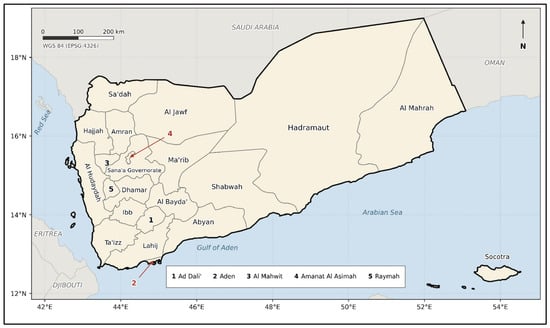
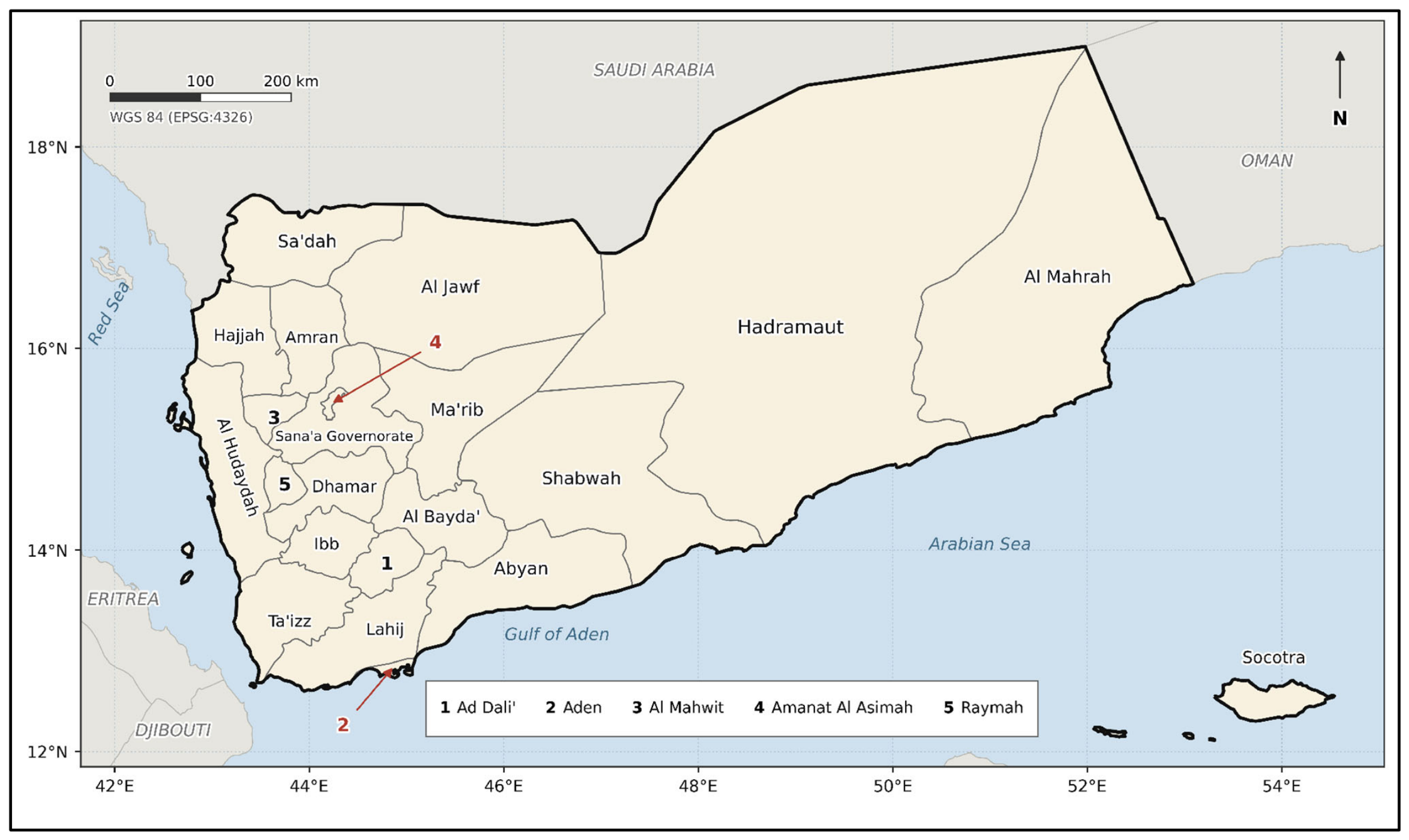
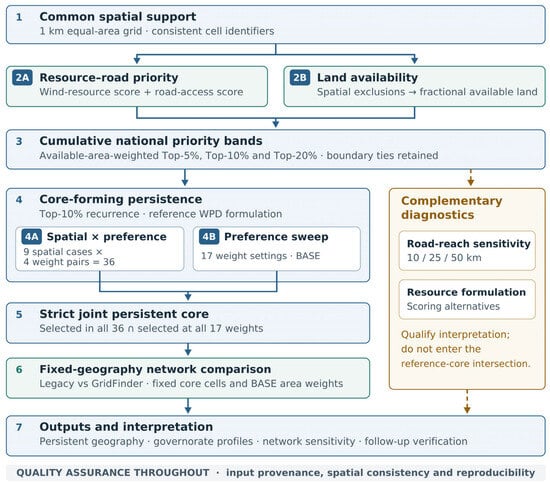
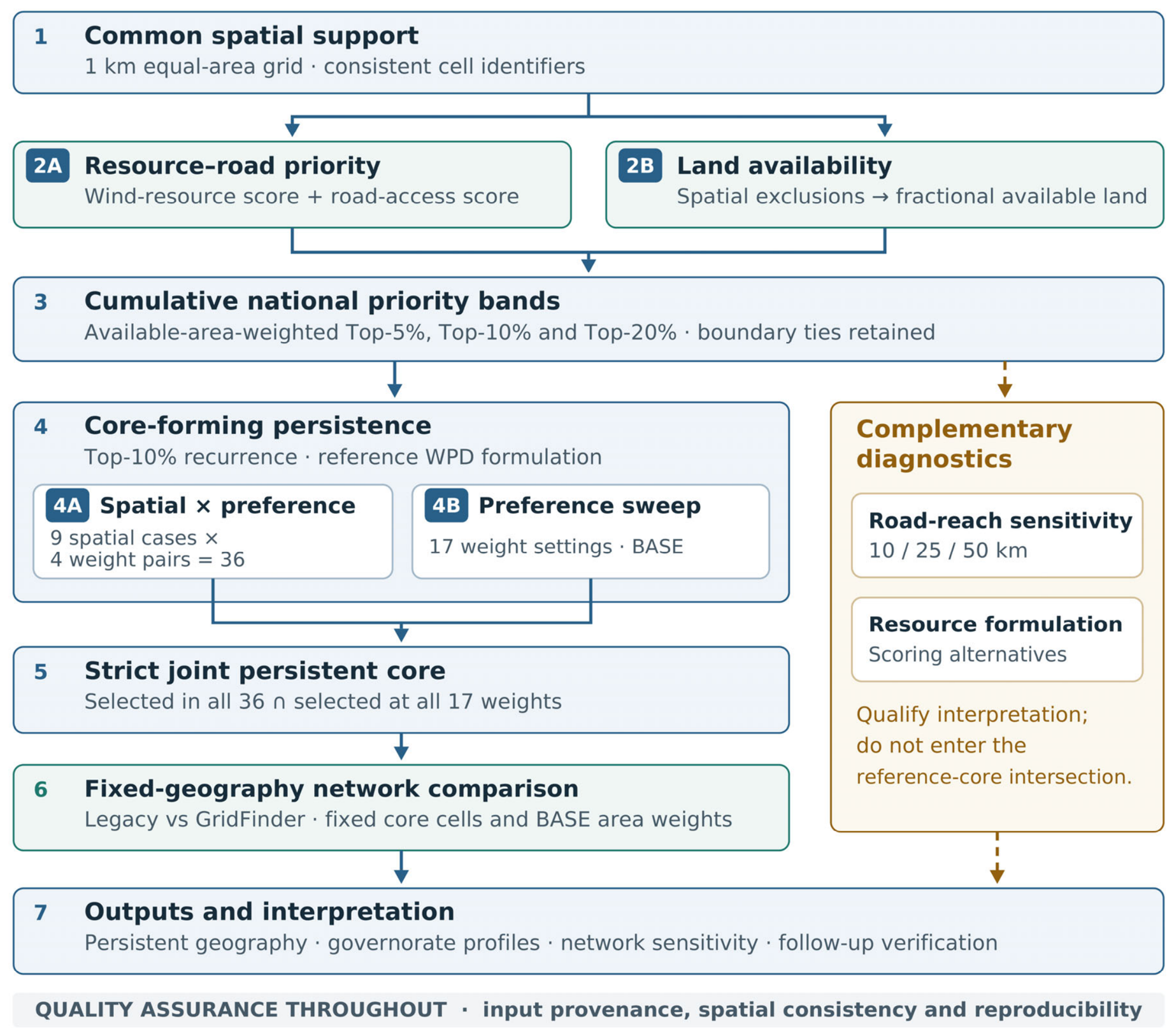
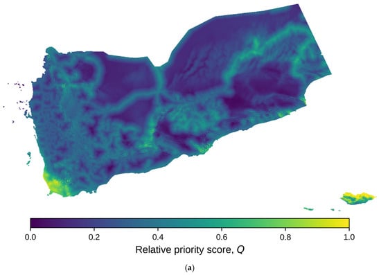
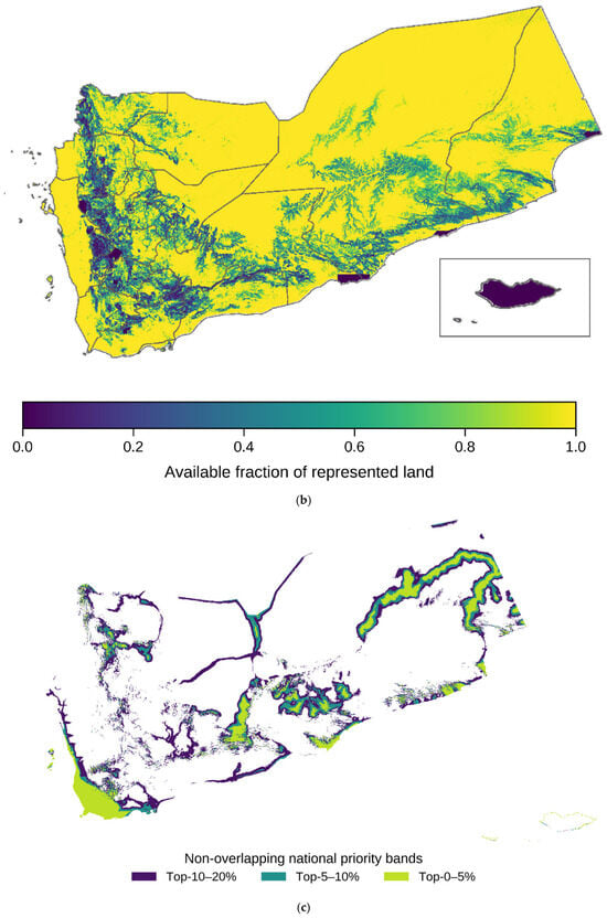
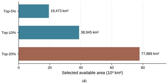
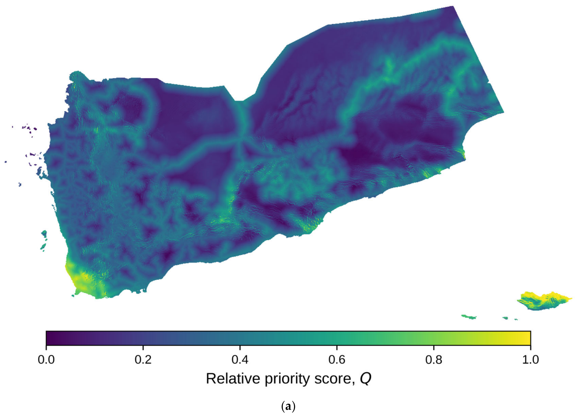
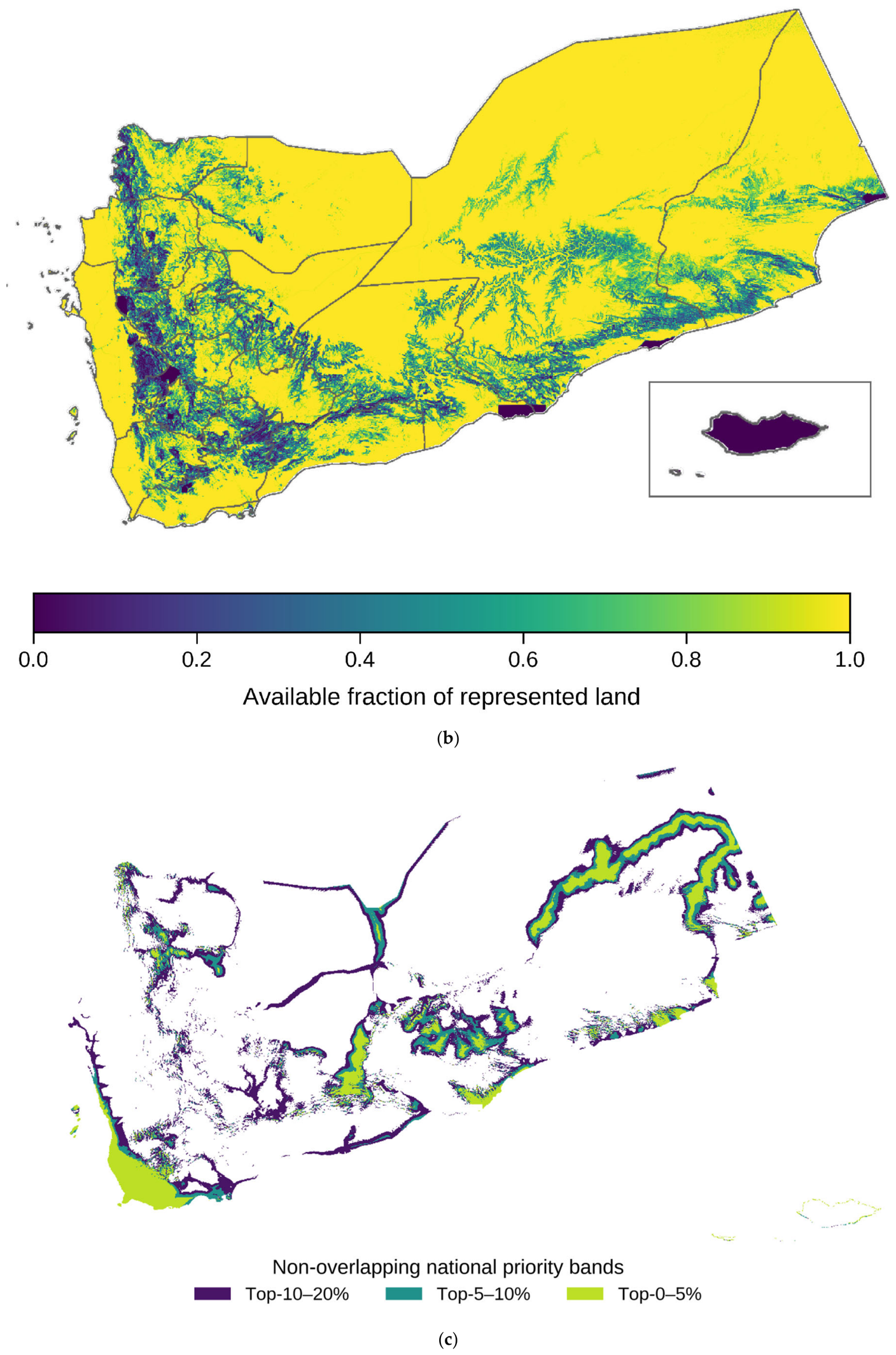
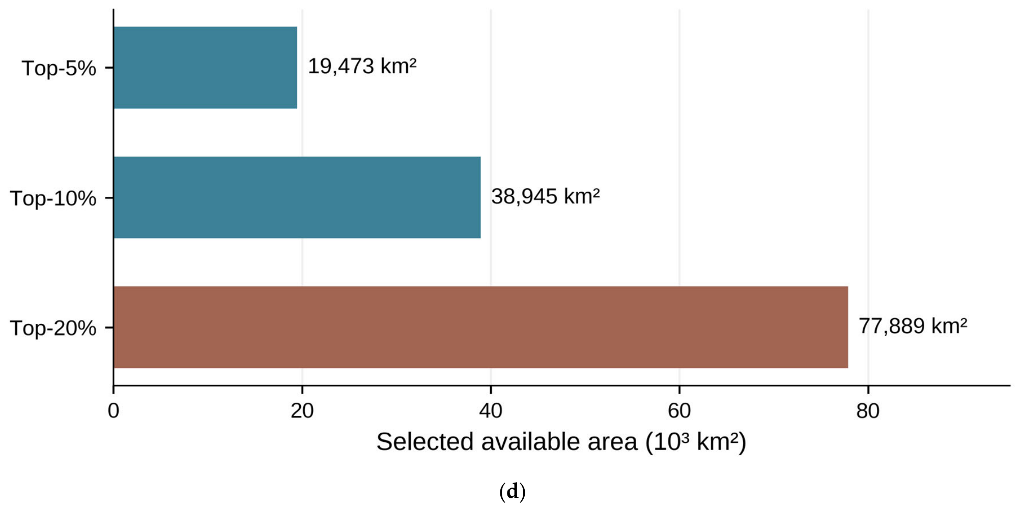
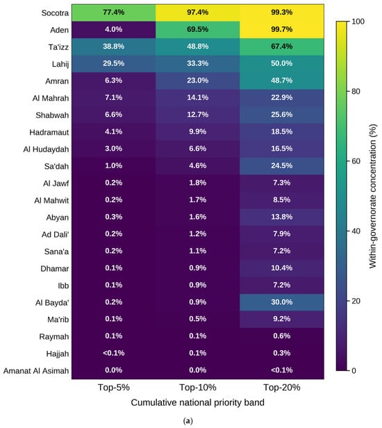
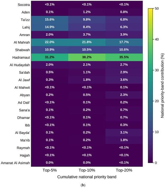
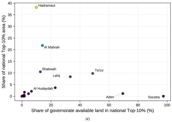
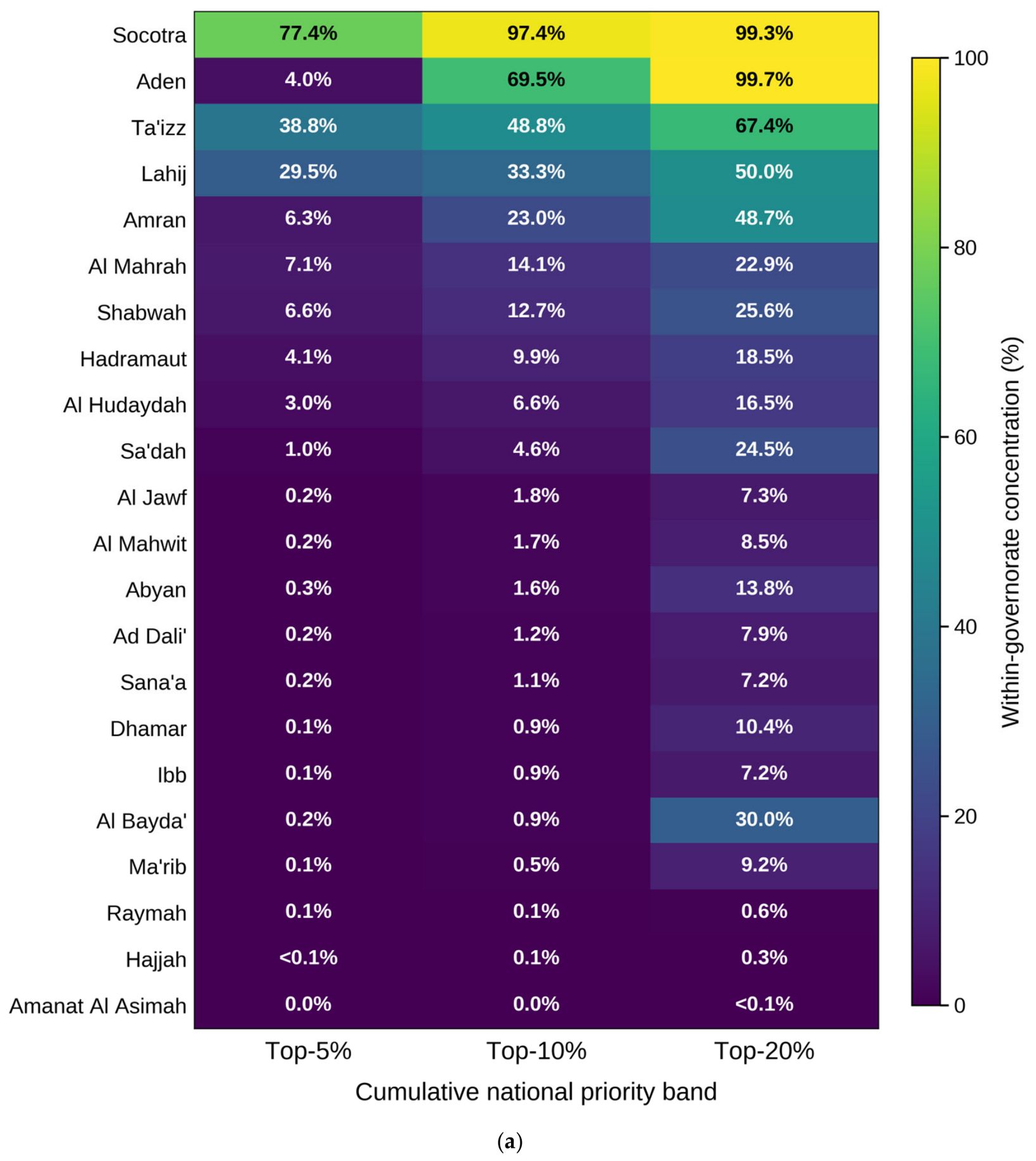
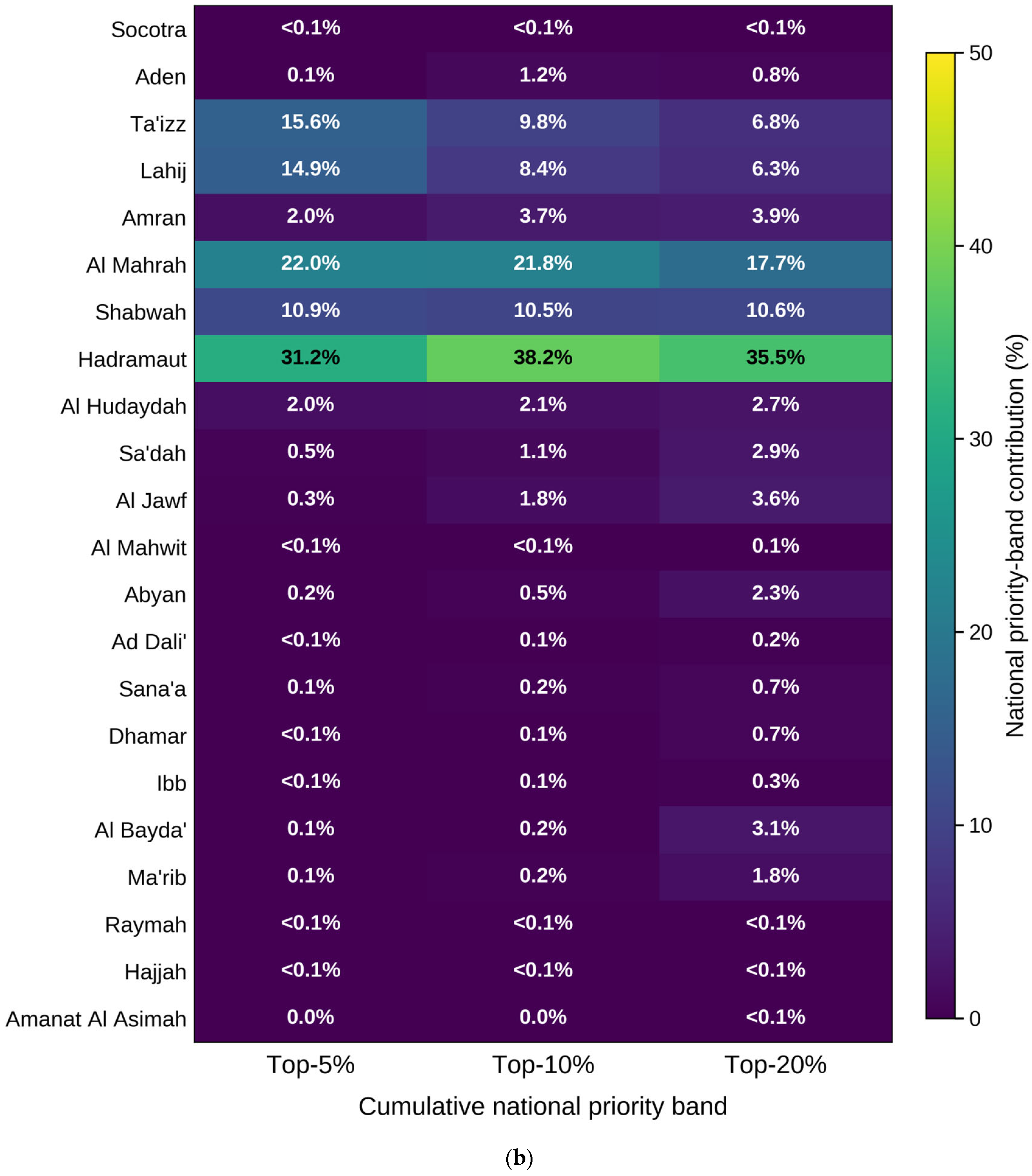
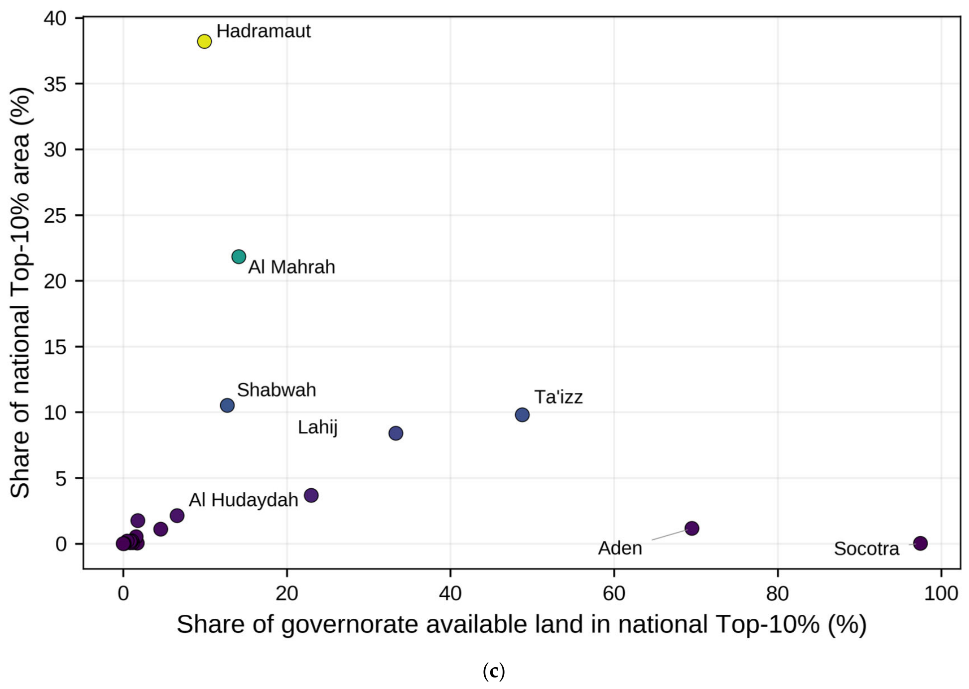
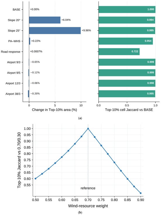
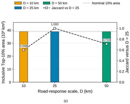
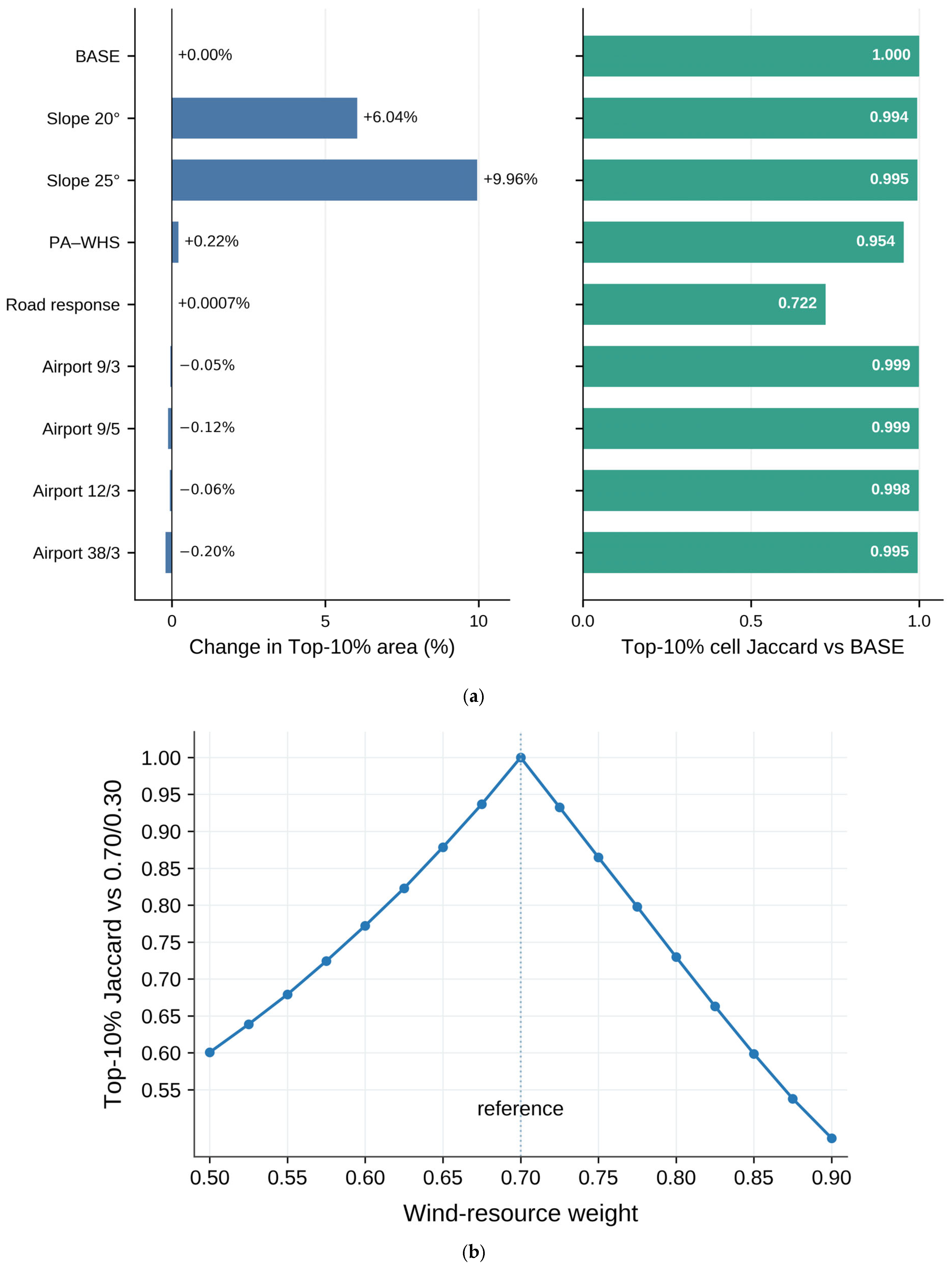
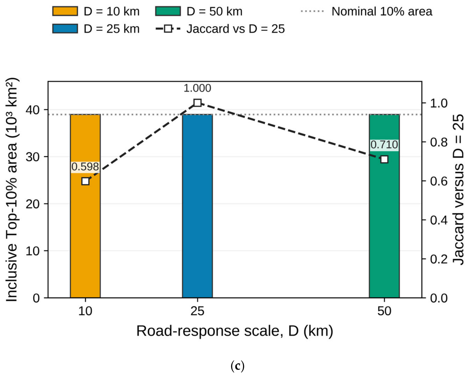
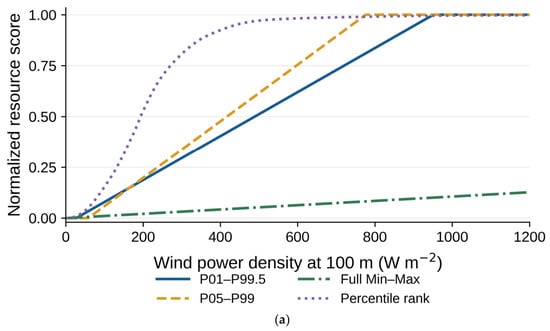
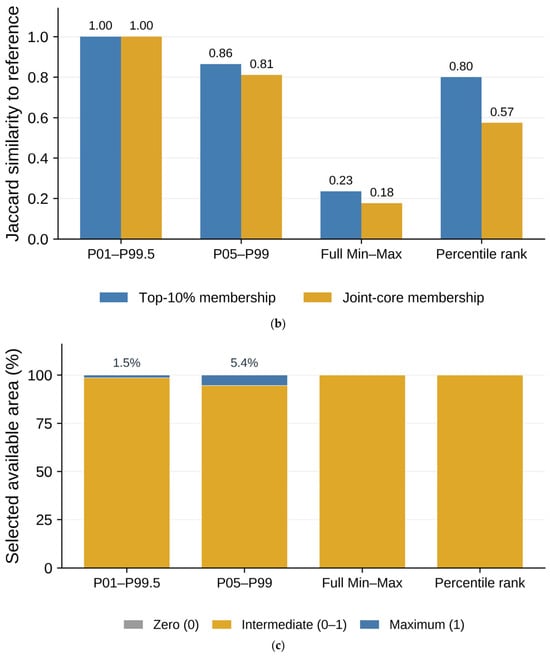
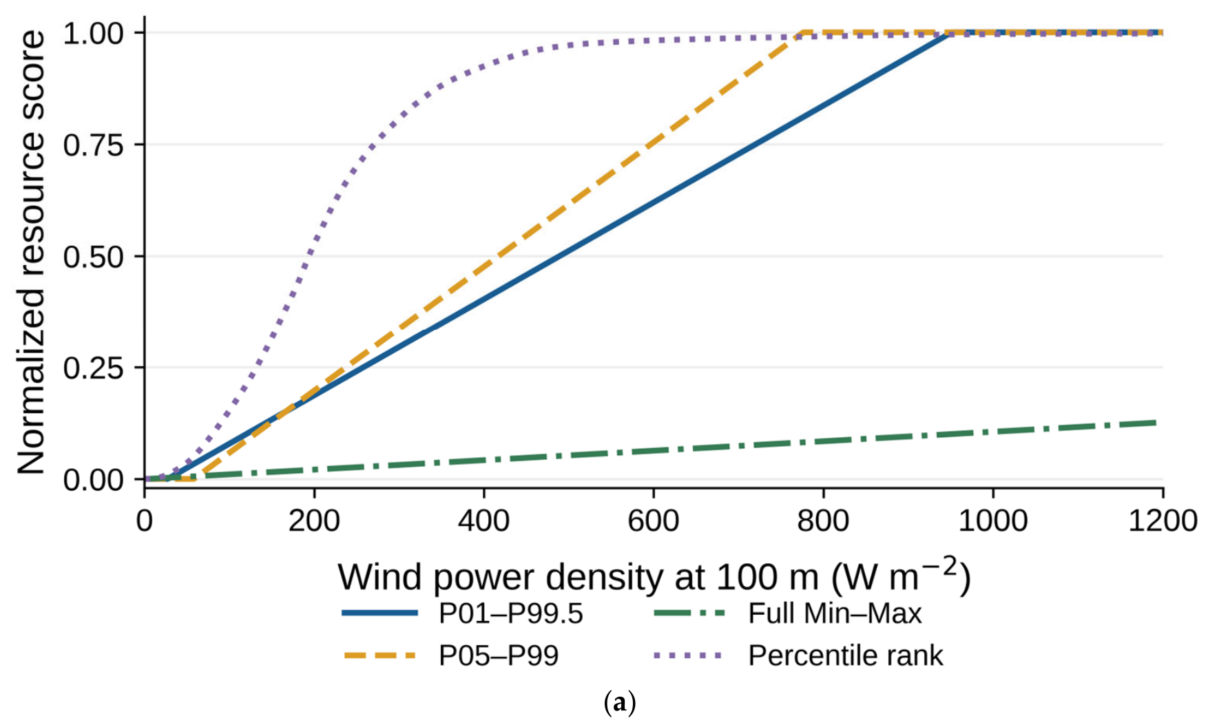
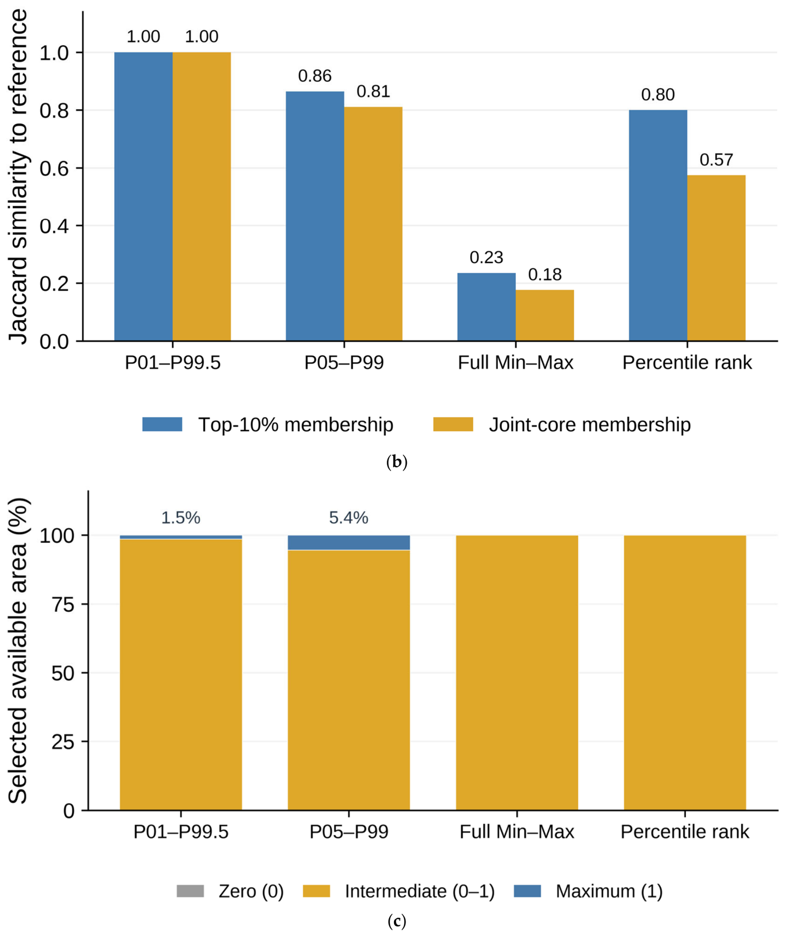
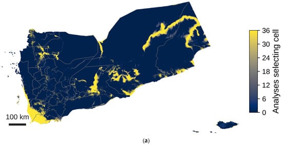
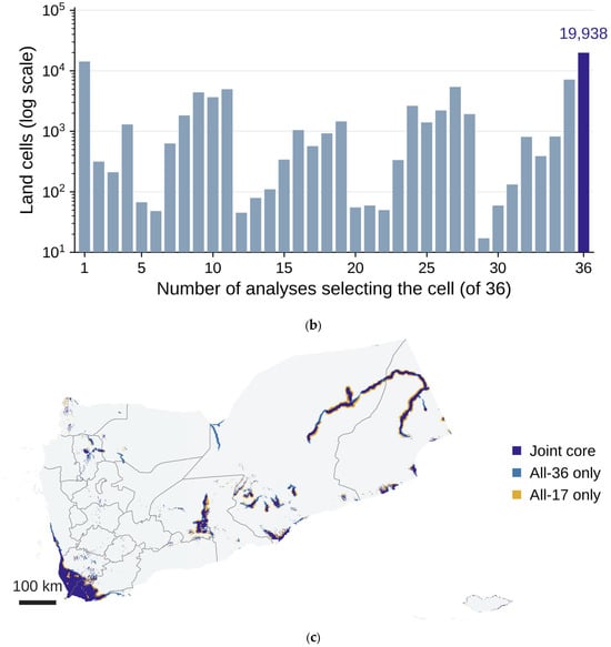
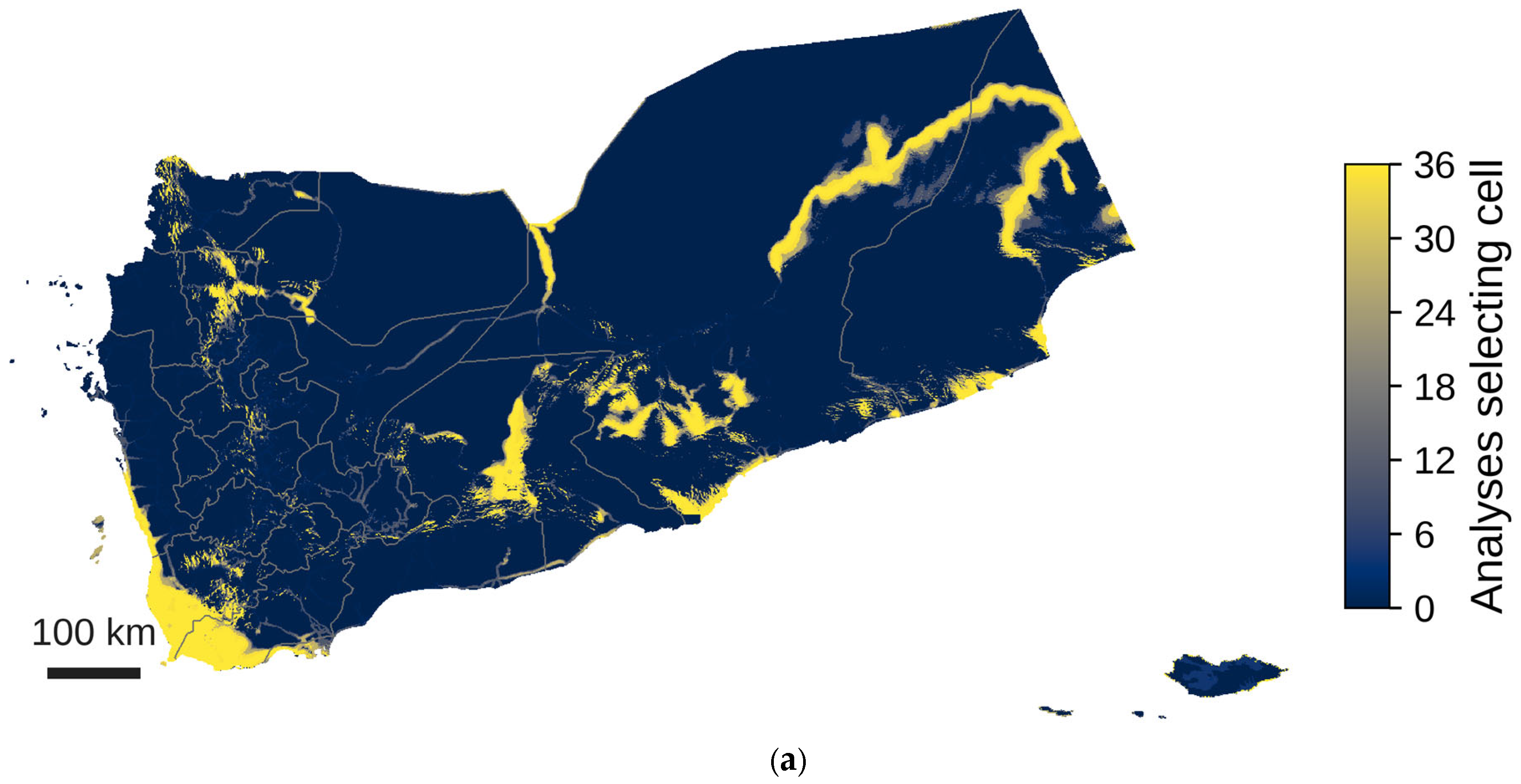
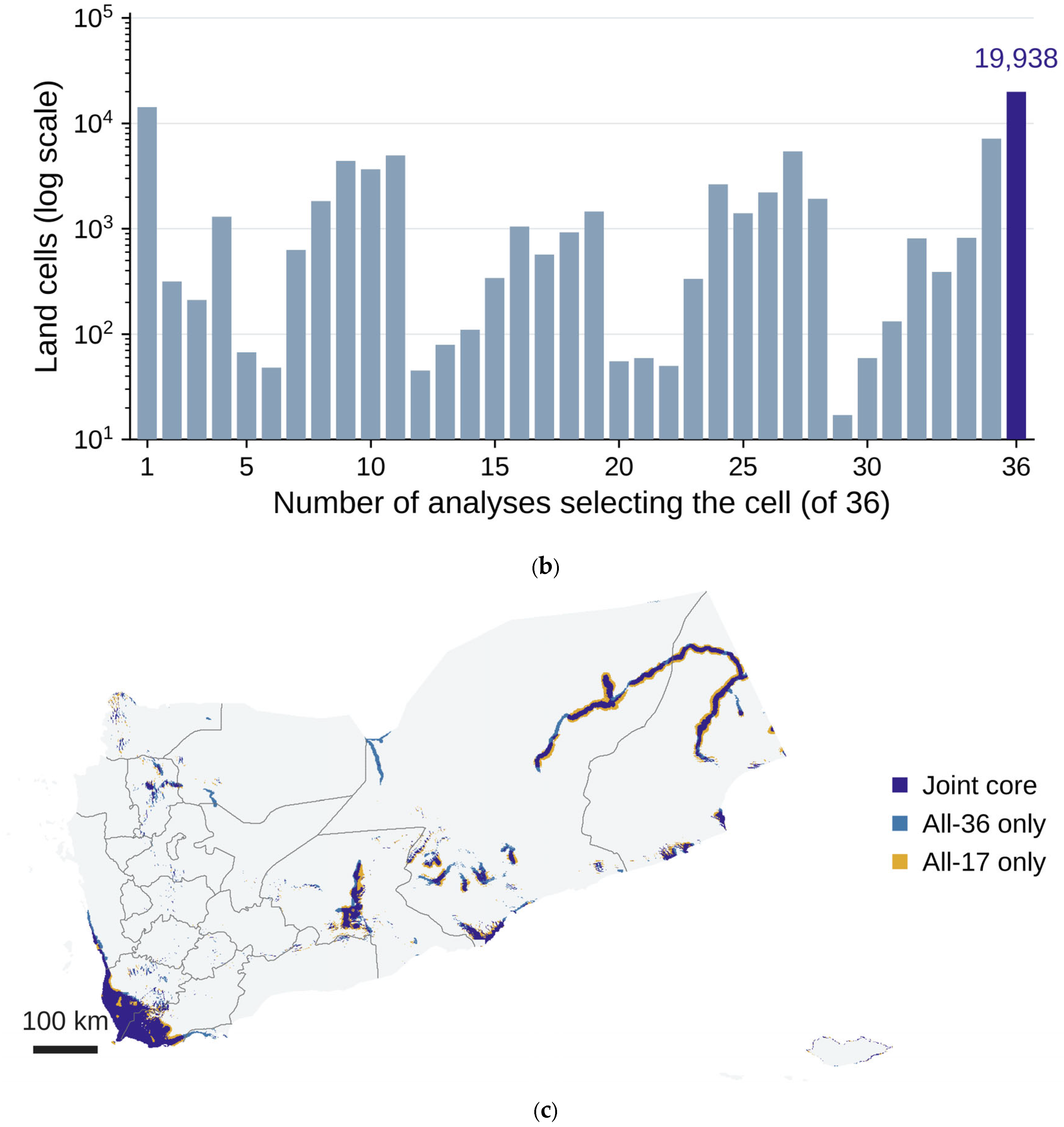
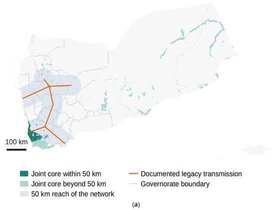
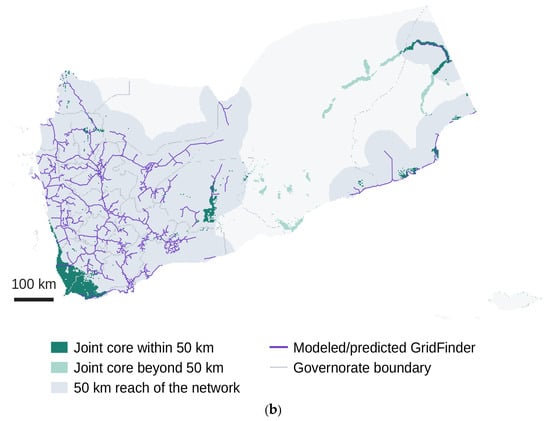
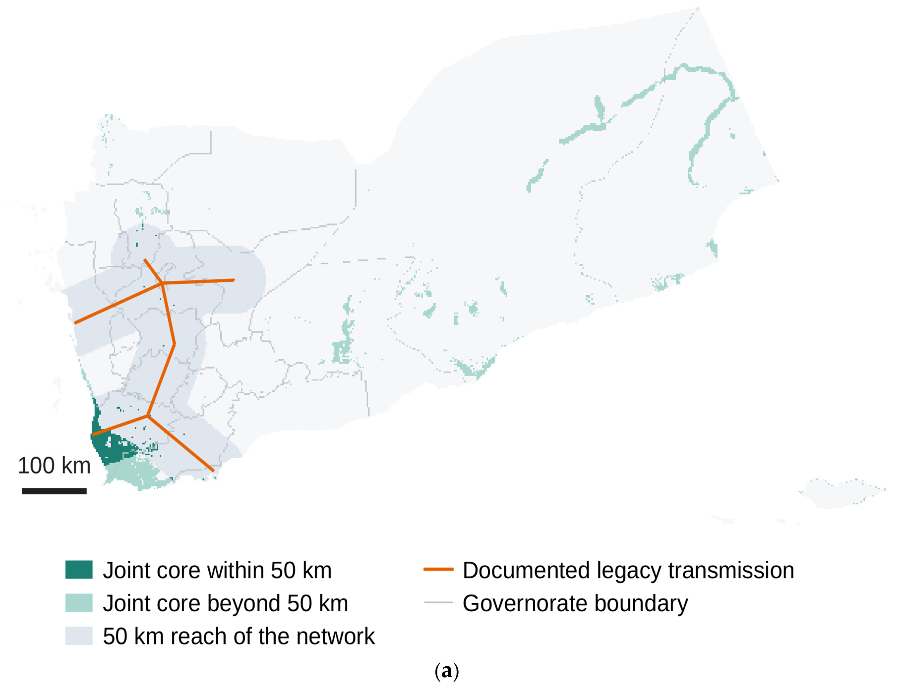
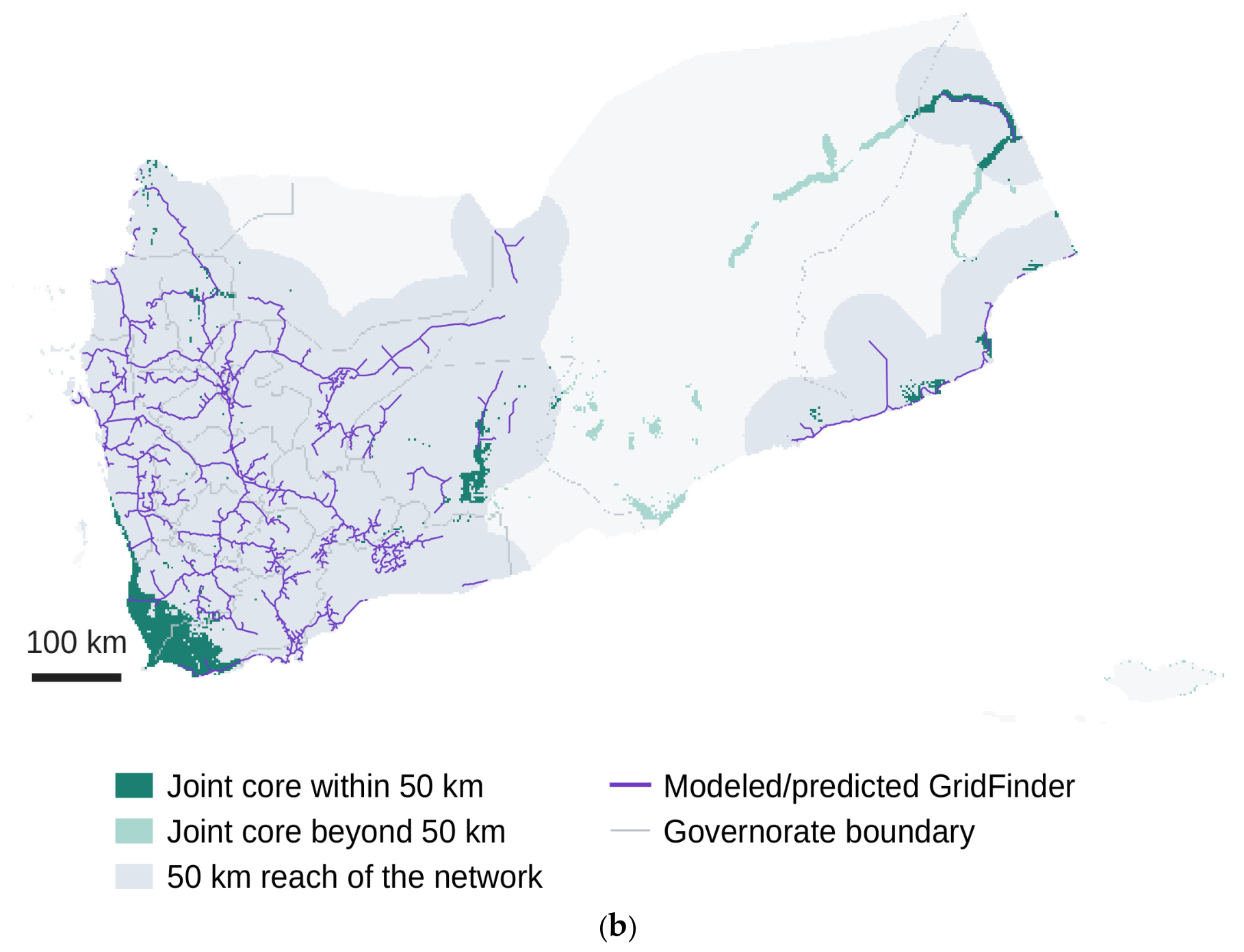

Disclaimer/Publisher’s Note: The statements, opinions and data contained in all publications are solely those of the individual author(s) and contributor(s) and not of MDPI and/or the editor(s). MDPI and/or the editor(s) disclaim responsibility for any injury to people or property resulting from any ideas, methods, instructions or products referred to in the content. |
© 2026 by the author. Licensee MDPI, Basel, Switzerland. This article is an open access article distributed under the terms and conditions of the Creative Commons Attribution (CC BY) license.