


Abstract
Partial shading deforms photovoltaic (PV) current–voltage (I–V) characteristics and complicates reliable condition monitoring. This study develops and stress-tests a compact, feature-based machine-learning framework using a public model-generated I–V dataset. The primary cohort contains 186 curves at 1000 W m−2, balanced across uniform operation and five nominal shading severities (10%, 20%, 30%, 40%, and 50%) at 31 temperatures from 20 to 50 °C. A verified set of 37 electrical, normalized, maximum-power-point, and curve-shape predictors was evaluated with six classifiers under 30 repeated stratified temperature-grouped five-fold validations, followed by nested grouped confirmation. The selected 10-feature logistic-regression model achieved 1.000 accuracy, balanced accuracy, macro-F1, Matthews correlation coefficient, Cohen’s κ, and ROC-AUC for binary and six-class diagnosis; the temperature-group bootstrap 95% confidence interval for macro-F1 was 1.000–1.000. A single normalized maximum-power-point-voltage predictor also achieved macro-F1 = 1.000, showing that the controlled source domain is strongly and partly rule-separable. The clean high-C solution was highly sensitive to measurement disturbance: under a 5% combined bias, drift, Gaussian, and quantization stress test, mean macro-F1 fell to 0.395 for binary detection and 0.095 for six-class diagnosis, whereas noise-aware training remained 0.976 and 0.962, respectively. Normalized maximum-power-point voltage, fill factor, maximum-power-point voltage, and maximum-power-point power were the dominant features. A uniform-operation negative control across 500–1000 W m−2 also exposed irradiance-domain sensitivity in the noise-aware model. The results establish reproducible controlled-domain discrimination and uncertainty sensitivity, but external measured-data validation across irradiance, modules, array configurations, and shadow geometries remains necessary before deployment.
1. Introduction
Photovoltaic generation is central to increasingly distributed, lower-carbon electricity systems [1,2,3,4,5,6,7]. Advances in module architecture, tracking, building integration, and device design have broadened PV deployment [8,9,10,11], while reliable operation still depends on timely diagnosis of disconnections, short circuits, bypass-diode failures, degradation, hot spots, soiling, and partial shading [12,13,14]. Partial shading is especially consequential because non-uniform irradiance changes the I–V and power-voltage (P–V) characteristics, displaces the usable maximum-power point (MPP), and may create multiple local maxima [15,16]. Data-driven PV diagnosis has consequently expanded across electrical, thermal, and image-based measurements [17,18,19], including I–V reconstruction and quantitative state evaluation [20,21,22]. The present benchmark includes established random-forest, support-vector-machine, and XGBoost methods [23,24,25], uses the public Mendeley dataset [26], and is positioned alongside recent Solar studies on thermal, vegetation, and AC-side anomalies [27,28,29]. Extra Trees and gradient boosting extend the ensemble comparison [30,31]. The associated source article states that the public curves were generated from a single-diode solar-PV model for emulator development [32]. Four issues motivate the revised study. First, model-generated or narrowly controlled datasets can yield optimistic performance when closely related operating conditions cross the training–test boundary. Second, a large feature space or complex classifier may add little when a small number of physically structured descriptors already separates the labels. Third, clean-data accuracy does not establish robustness to bias, drift, quantization, correlated error, or irradiance-domain shift. Fourth, practical condition monitoring requires an explicit account of I–V acquisition hardware, scan interruption, and the economic opportunity cost of moving an array away from maximum-power operation. The revised framework therefore treats partial-shading diagnosis as a combined discrimination, leakage-control, uncertainty, and deployment problem:
- The primary contribution is a reproducible analysis of 186 model-generated I–V curves at 1000 W m−2 across six balanced operating states, with all six records associated with one temperature retained in the same validation fold.
- The verified modelling matrix contains 37, rather than 45, predictors. These are documented individually and organized into core (10), no-local-peak (22), shape (17), and full (37) representations, with parsimonious one-feature and shallow-tree benchmarks.
- Model comparison uses 30 repeated stratified temperature-grouped five-fold evaluations, temperature-group bootstrap confidence intervals, exploratory paired tests, and five-outer/four-inner nested grouped confirmation.
- Deployment sensitivity is assessed using Gaussian random error, fixed bias, drift, quantization, correlated error, and a combined disturbance across multiple magnitudes. The revision also reports class-level confusion patterns, a uniform-only cross-irradiance negative control, practical acquisition pathways, and illustrative scan-interruption economics.
Section 2 describes dataset provenance, the analytical cohort, features, and related studies. Section 3 presents reconstruction, grouped validation, statistical analysis, model selection, explanation, uncertainty testing, and reproducibility procedures. Section 4 reports discrimination, robustness, physical interpretation, cross-condition findings, deployment implications, and limitations. Section 5 concludes the study.
2. Data Basis and Related Work
2.1. Dataset Provenance, Generation, and Analytical Cohort
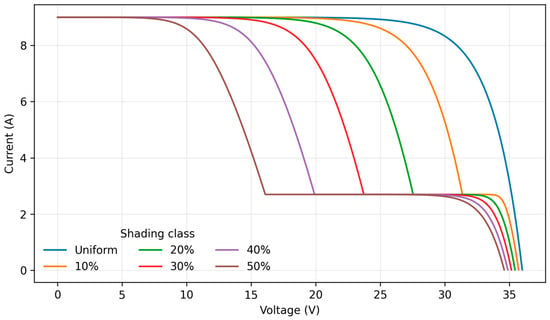
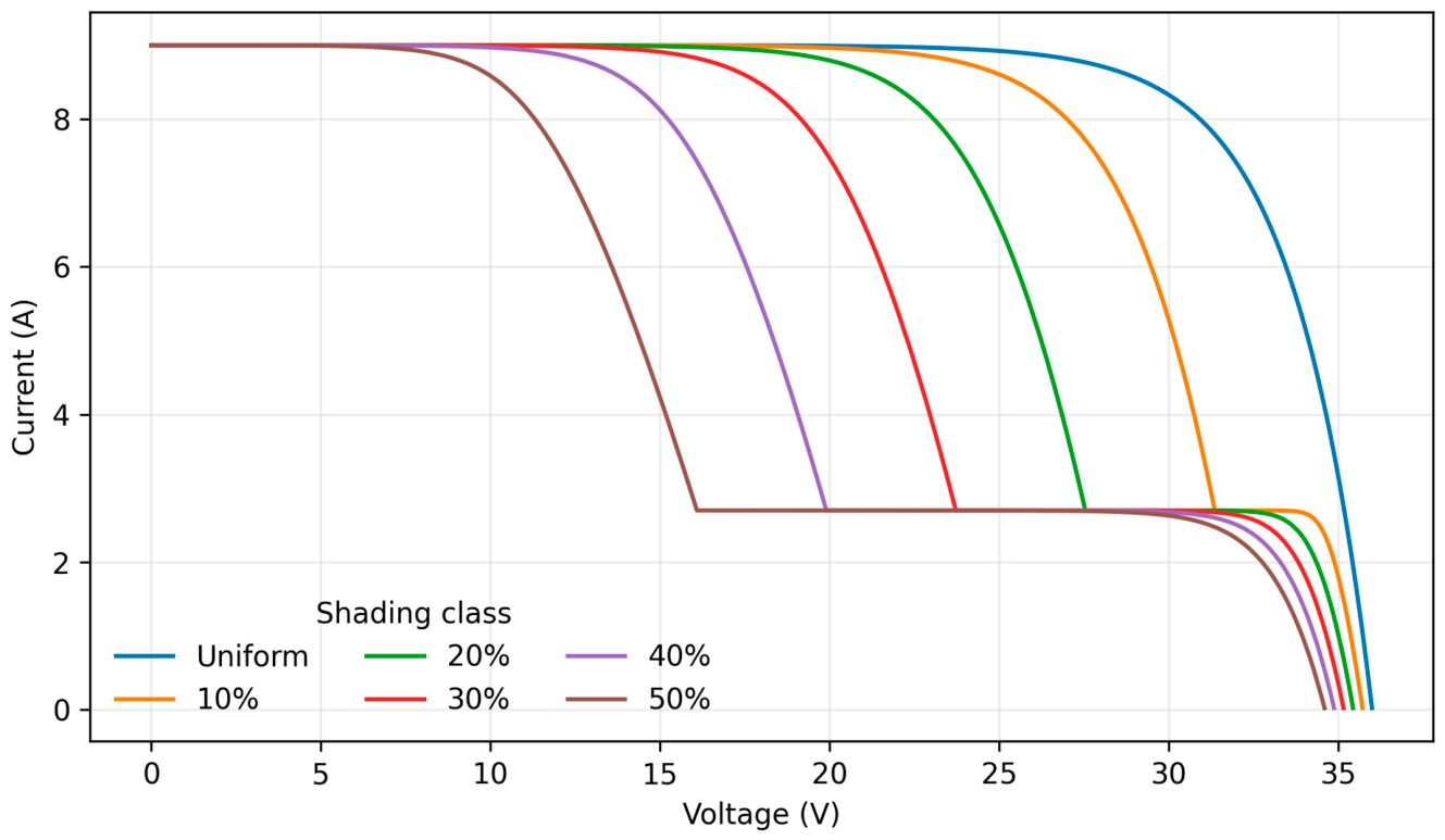
The study uses Version 1 of “PV Panel: Irradiance, Temperature, Partial Shading-IV Curves” [26]. The associated article reports that the training data were generated using a single-diode solar-PV model developed for a photovoltaic emulator [32]. The released uniform-operation domain spans irradiance from 500 to 1000 W m−2 in 50 W m−2 steps and temperature from 20 to 50 °C. The partial-shading file uses two irradiance regions, 300 and 1000 W m−2, over the same temperature range and provides nominal shading labels of 10%, 20%, 30%, 40%, and 50% (see Figure 1). The source illustrates a 60-cell panel and 12- and 24-cell shaded examples, but does not report a manufacturer-specific module datasheet, I–V tracer, scan duration, bypass-diode topology, independent shadow-pattern identifier, site, day, or replicate identifier. These unavailable details are not inferred.
Figure 1.
Representative model-generated I–V curves for the six analyzed classes at 25 °C and 1000 W m−2; voltage is in volts, and current is in amperes.
The primary analysis retains the 186 records at 1000 W m−2 so that irradiance cannot act as a direct class proxy. The cohort contains 31 temperature-matched records in each of six classes: Uniform, 10%, 20%, 30%, 40%, and 50% partial shading. The percentage labels are reported exactly as supplied by the dataset creators; because an independent spatial shadow-pattern identifier is unavailable, the study does not claim validation across different geometries at the same nominal severity. Table 1 summarizes the source and analytical cohort, while Appendix A Table A1 provides the full provenance audit. The raw curve files and supplied operating-point quantities were cross-checked before feature extraction. No exact duplicate rows, duplicate core-feature vectors, or conflicting feature-label vectors were found in the 186-record primary cohort. This audit reduces, but does not eliminate, the risk that the models reproduce the source generation rule rather than transferable physical variation. The dataset is therefore treated as a controlled model-generated benchmark, not as a field-measurement campaign. All claims in this paper are confined to the represented source domain unless an explicit negative-control or stress-test result is reported.
Table 1.
Public-dataset provenance, source-domain information, and the primary analytical cohort.
2.2. Predictor Variables and Diagnostic Targets
The released modelling matrix was audited against the extraction code and contains 37 predictors. Table 2 summarizes the four predefined representations; Appendix A Table A2 lists every predictor, definition or extraction procedure, unit, and physical interpretation. The compact core representation contains irradiance G (W m−2), temperature T (°C), open-circuit voltage V_OC (V), short-circuit current I_SC (A), global maximum-power-point voltage V_MP (V), current I_MP (A), power P_MP (W), fill factor FF (dimensionless), normalized MPP voltage V_MP/V_OC, and normalized MPP current I_MP/I_SC. The targets are binary (Uniform versus Partial shading) and six-class (Uniform and five nominal severities).
Table 2.
Predefined feature representations. The complete 37-predictor inventory, definitions, procedures, and units are provided in Appendix A Table A2.
The six-class target retains nominal shading severity, whereas the binary target evaluates general shading detection. Irradiance is constant in the primary cohort but remains in the schema so that the released feature pipeline is documented exactly. It contributes no within-cohort variance and is not interpreted as a diagnostic driver.
2.3. Feature Inventory and Physical-Consistency Audit
The 37 predictors comprise operating conditions, supplied and reconstructed electrical landmarks, global and local MPP descriptors, normalized ratios, curve areas, derivative and curvature measures, peak widths, and related shape indicators. The core, no-local-peak, shape, and full representations contain 10, 22, 17, and 37 predictors, respectively. Dense I–V reconstruction reproduced V_OC and I_SC exactly. P_MP showed a mean absolute error of 0.002694 W, a root-mean-square error of 0.003284 W, and a maximum absolute error of 0.009175 W.
The controlled design isolates severity-related electrical changes at a common irradiance while retaining temperature variation for grouped validation. As nominal severity increases, current delivery, MPP position, fill factor, and curve morphology change systematically. These effects provide the physical basis for the feature space, but the strong ordering also motivates explicit one-feature and leakage diagnostics.
2.4. Related Work and Quantitative Positioning
PV fault diagnosis has progressed from threshold-based electrical monitoring to machine-learning methods that combine electrical, environmental, thermal, and imaging measurements [12,13,14,15,16,17,18,19]. I–V and P–V characteristics are particularly relevant to partial shading because they retain open- and short-circuit landmarks, the MPP, fill factor, knee deformation, and local-power-peak structure [15,16,20]. Recent research has also investigated quantitative state evaluation under uncertain shading [19], I–V reconstruction for partial-shading assessment [20], interpretable feature selection [21,22], and edge-oriented real-time fault diagnosis [33]. Table 3 compares selected studies using dataset basis, class scope, inputs, validation, and reported quantitative performance. Direct ranking is inappropriate because the studies use different modules, fault taxonomies, class balances, and split designs. The present contribution is therefore not a new classifier alone; it is the combination of verified feature accounting, temperature-grouped and nested validation, parsimonious baselines, uncertainty stress testing, class-level analysis, and explicit deployment boundaries. A recent dual-channel spatiotemporal model reported 94.69% accuracy and macro-F1 = 0.9413 on seven PV-plant fault classes [34], illustrating the different scale and complexity of field-oriented time-series diagnosis.
Table 3.
Quantitative positioning against selected photovoltaic fault- and partial-shading-diagnosis studies. Metrics are not directly comparable because datasets, targets, and validation designs differ.
The comparison shows why perfect internal classification on a controlled source should be interpreted together with feature discriminability, uncertainty sensitivity, and external-validity limits. The revised evaluation therefore reports both the favourable clean-data result and the conditions under which it fails.
3. Materials and Methods
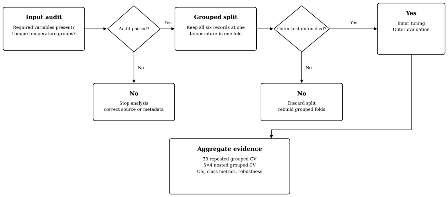
The revised workflow contains four linked stages: source and cohort audit (Figure 2), verified feature construction and dual diagnostic tasks (Figure 3), leakage-controlled nested decision logic (Figure 4), and explanation/uncertainty/deployment evaluation (Figure 5). Every transformation that can learn from the data, including imputation, scaling, model selection, and augmentation, is fitted within the corresponding training partition.
Figure 2.
Dataset eligibility, provenance, curve reconstruction, and physical-consistency audit. Decision outcomes that fail an integrity check return to source verification.
Figure 3.
Verified feature-engineering and binary/six-class classification workflow. Feature counts refer to the audited 37-predictor matrix.
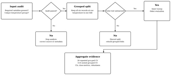
Figure 4.
Leakage-controlled grouped and nested validation with explicit yes/no decision branches for data integrity, temperature-group separation, inner selection, outer evaluation, and robustness escalation.
Figure 5.
Explainability, multi-mechanism sensor-error stress testing, cross-condition negative control, class-level analysis, and deployment interpretation.
3.1. Data Partitioning, Grouping Rationale, and Normalization
The analyzed cohort contains n = 186 model-generated I–V records and p predictors. Each of the 31 temperatures has one observation from every class. Temperature is therefore the only available operating-condition identifier that creates matched six-record groups; all records from one temperature are assigned wholly to either training or testing. This prevents temperature-matched observations from crossing the fold boundary. Irradiance is fixed at 1000 W m−2 in the primary cohort, severity is the prediction target, and no independent module, site, day, replicate, or shadow-pattern identifier is released:
The target vector in Equation (2) represents either Uniform versus Partial shading or the six nominal severity states. The labels are dimensionless categorical variables:
Four representations are evaluated: core (10 predictors), no-local-peak (22), shape (17), and all features (37). Missing values are imputed using training-fold medians. Logistic regression and RBF-SVM are standardized using training-fold statistics according to Equation (3); tree-based models use median imputation without scaling:
For feature j, xij has the unit of the original feature, while the training-fold mean μj and standard deviation σj have the same unit. Their standardized value zij in Equation (3) is dimensionless. The fitted μj and σj are applied unchanged to held-out temperature groups. The full symbol-and-unit register is given in Appendix A.6.
3.2. Raw-Curve Reconstruction and Physical Audit
For each class-temperature combination, repeated model outputs at common voltage points were averaged, ordered by increasing voltage, and interpolated onto a 2001-point grid from 0 V to V_OC (V). The current I(V) is in amperes, and the reconstructed power P(V) = V I(V) is in watts. The global maximum is the point with the largest P(V), producing V_MP in volts, I_MP in amperes, and P_MP in watts:
P(V) = VI(V)
Equation (5) defines V_MP (V), I_MP (A), and P_MP (W). Reconstructed endpoints and global MPP quantities were compared with the supplied summary records using MAE, RMSE, and MaxAE in the corresponding physical unit, and Pearson r as a dimensionless association measure. This audit verifies consistency within the public source; it is not an independent laboratory validation.
3.3. Feature Engineering
The 37 predictors describe operating conditions, electrical endpoints, global and local MPP landmarks, dimensionless ratios, integrated I–V/P–V areas, derivatives, curvature, peak widths, and related shape properties. Appendix A Table A2 provides the definitive inventory. Fill factor is defined in Equation (6), normalized MPP voltage and current in Equations (7) and (8), integrated areas in Equations (9) and (10), and curvature in Equation (11):
In Equation (6), FF is dimensionless, P_MP is in watts, V_OC is in volts, and I_SC is in amperes. V_MP/V_OC in Equation (7) is dimensionless:
Equation (8) gives I_MP/I_SC, also dimensionless. The two ratios locate the MPP relative to the I–V endpoints and reduce dependence on absolute electrical scale:
Equation (9) gives the I–V area in watt-equivalent units (V·A), and Equation (10) gives the P–V area in W·V. Numerical integration is applied to the unsmoothed interpolated curves:
Savitzky–Golay smoothing is used only for derivative estimation. Equation (11) defines I–V curvature; its numerical dimension depends on the voltage–current scaling used for the curve, so it is interpreted comparatively after standardized preprocessing rather than as a standalone physical constant:
The core, no-local-peak, shape, and full representations contain 10, 22, 17, and 37 predictors, respectively. They are specified before model comparison and are not selected using held-out performance.
3.4. Classification Tasks and Models
Two tasks are evaluated: binary Uniform-versus-Partial-shading detection and six-class severity diagnosis. The benchmark comprises logistic regression (LR), radial-basis-function support-vector machine (RBF-SVM), random forest [23], Extra Trees [30], HistGradientBoosting [31], and XGBoost [25]. A logistic model using only normalized MPP voltage and a shallow decision tree are added as parsimonious baselines.
LR and RBF-SVM use median imputation followed by standardization. Equation (12) defines dimensionless zij from feature value xij and the training-fold μj and σj; xij, μj, and σj share the physical unit of feature j:
The symbols xij, μj, σj, and zij follow the same italic/subscript convention in prose and Equation (12). Held-out observations never contribute to these preprocessing parameters.
For binary logistic regression, the probability of partial shading is modelled by Equation (13):
Equation (13) uses an intercept and a coefficient vector acting on the standardized predictor vector. For six-class diagnosis, class probabilities are obtained using the softmax model in Equation (14).
For multiclass diagnosis, the probability assigned to class k is defined by Equation (14):
In Equation (14), K = 6, and each class has an intercept and coefficient vector. Logistic models are estimated by minimizing regularized cross-entropy as expressed in Equation (15).
The regularized objective used for logistic regression is given in Equation (15):
In Equation (15), yik and pik are dimensionless class indicator and probability values, respectively; C is the dimensionless inverse regularization strength. Larger C corresponds to weaker L2 regularization.
3.5. Repeated Grouped Validation, Uncertainty, and Performance Metrics
All 48 task–feature–model combinations (2 tasks × 4 feature sets × 6 classifiers) are evaluated over 30 repeated stratified grouped five-fold experiments. Temperature is the grouping variable, yielding 1440 repeat-level evaluations and 267,840 out-of-fold predictions. The repeated folds reuse observations and are therefore interpreted as resampling-stability evidence, not as 30 independent datasets. Principal confidence intervals use 5000 bootstrap resamples of the 31 temperature groups.
Primary performance measures are macro-F1, balanced accuracy, and log loss. The class-specific F1 score is defined in Equation (16):
Precision and recall are computed for each class, and macro-F1 is the unweighted mean of the class-specific F1 scores, as defined in Equation (17):
Balanced accuracy is the mean class recall and is defined in Equation (18). It gives each class equal contribution regardless of class frequency:
True-positive and false-negative counts are evaluated class-wise. Probability quality is assessed with multiclass log loss, defined in Equation (19), which penalizes confidently incorrect predictions:
Equation (19) defines dimensionless log loss. Lower values indicate better probability assignment, but extremely low clean-data loss can also reflect near-separable source labels and should not be equated automatically with deployment calibration. The leakage-control condition for temperature-grouped validation is stated in Equation (20):
Equation (20) requires the training and test temperature-group sets to be disjointed in every fold. Additional metrics are accuracy, weighted F1, macro precision, macro recall, MCC, Cohen’s κ, and one-versus-rest ROC-AUC; all are dimensionless. The same grouped partitions are applied to the one-feature and shallow-tree baselines. Class-wise precision, recall, and F1 are reported for the combined 5% disturbance condition to identify which nominal severities become confusable.
3.6. Statistical Comparisons and Nested Confirmation
Mean performance uncertainty is quantified by temperature-group bootstrap intervals. Friedman and paired Wilcoxon–Holm analyses across repeated folds are retained as exploratory paired-resampling comparisons because folds and repetitions reuse observations. Rank-biserial correlation is reported as an effect-size descriptor. The corresponding statistics in Equations (21)–(23) are dimensionless:
3.7. Parsimony Rule and Nested Grouped Hyperparameter Confirmation
Candidate configurations are ranked by descending mean macro-F1, then ascending feature count, a predefined model-complexity order, and lower log loss. This selects the 10-feature LR model for both tasks. Nested validation uses five outer and four inner temperature-grouped folds. Each outer training set evaluates 500 random candidates over C ∈ [10−4, 104], tolerance ∈ [10−6, 10−3], class weighting, and intercept inclusion. A separate 500-candidate grouped search fits each final full-data model.
3.8. Explainability, Sensor-Error Stress Tests, and Cross-Condition Checks
Explainability uses standardized LR coefficients and 100-repeat permutation importance within nested outer test folds. The original perturbation protocol applies multiplicative zero-mean Gaussian error to primitive quantities. The revision additionally evaluates fixed bias, linear drift, quantisation, correlated random error (correlation coefficient 0.8), and a combined disturbance at 1%, 3%, 5%, and 10%. Derived FF and normalized MPP ratios are recomputed after perturbing primitive electrical quantities. Appendix A Table A3 defines every mechanism and clarifies that these are controlled stress tests, not a certified error model for a particular I–V tracer. Three deployment variants are compared: the clean high-C solution, a conventionally regularized C = 1 model, and a C = 1 model trained with five independently perturbed 2% copies of each training fold. Augmentation is confined to training data. Matched and mismatched disturbance types are assessed so that robustness is not inferred solely from identical training and test noise distributions. A limited cross-irradiance negative control applies the binary models to the available Uniform records from 500 to 1000 W m−2. Because lower-irradiance partial-shading records do not form a matched severity panel, this analysis can detect false-positive sensitivity only; it cannot establish severity generalization:
3.9. Reproducibility and Implementation
The executable workflow, random seeds, extracted features, predictions, disturbance outputs, and audit tables are retained in the revision package. To reduce main-text density, the detailed procedural algorithm requested for reproducibility is presented as Algorithm A1 in Appendix B rather than in the principal Methods section.
4. Results and Discussion
The results are interpreted in five layers: source integrity and curve agreement; clean grouped discrimination; statistical and nested confirmation; physical explanation; and uncertainty/cross-condition deployment evidence. This separation is necessary because excellent clean performance in a model-generated source does not imply universal field generalization.
4.1. Cohort Integrity and Raw-Curve Agreement
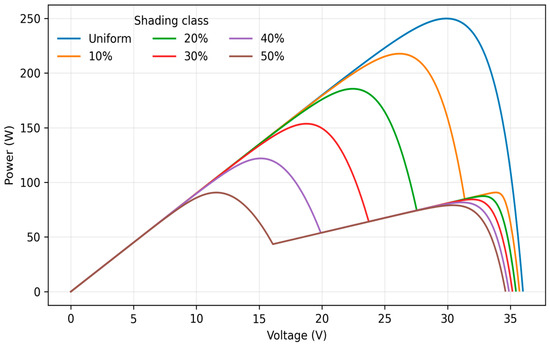
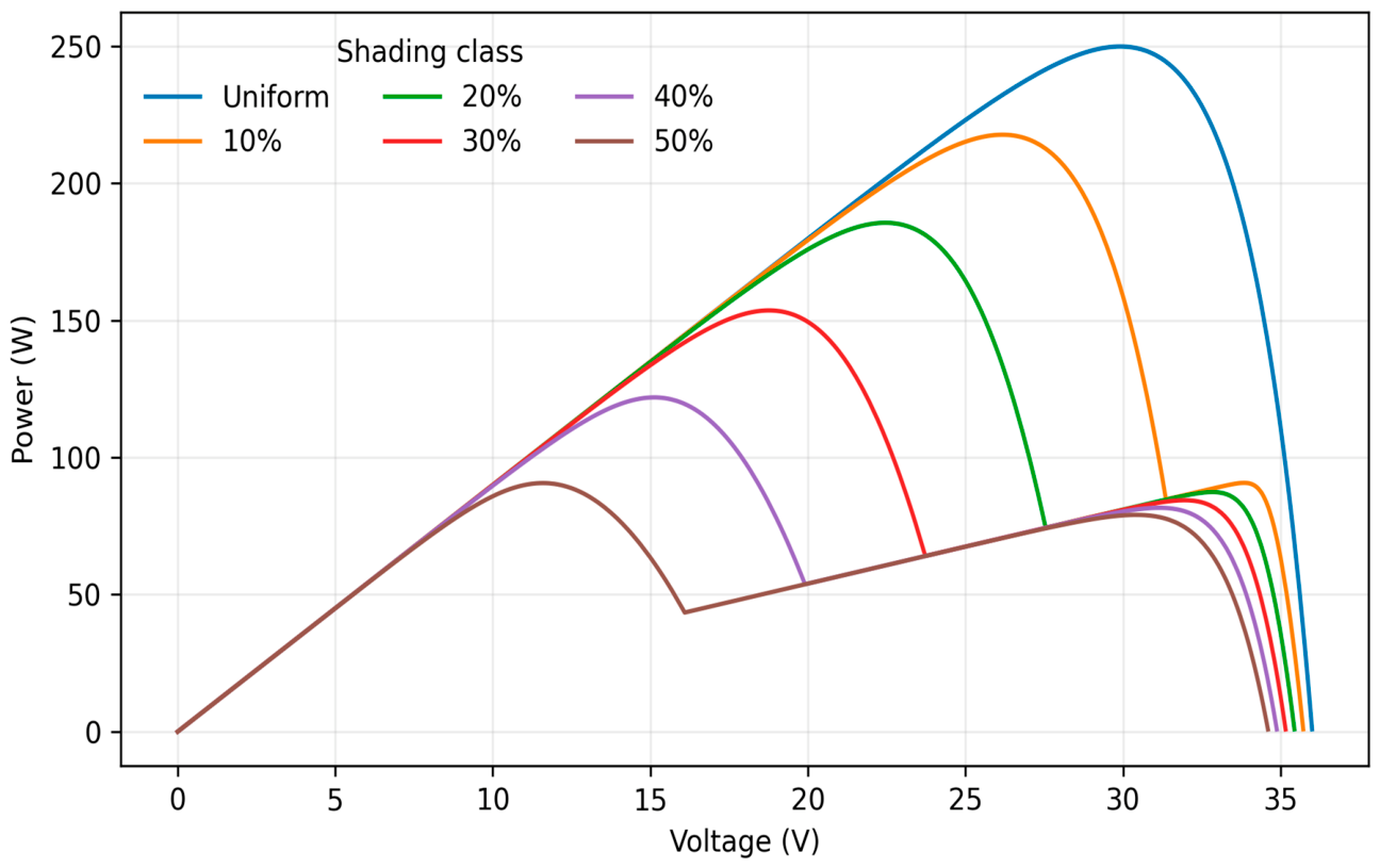
The primary cohort contains 186 model-generated curves, 31 observations in each class, and 31 non-overlapping temperature groups. Irradiance is fixed at 1000 W m−2. Dense reconstruction reproduces V_OC and I_SC exactly; P_MP has MAE = 0.002694 W, RMSE = 0.003284 W, and MaxAE = 0.009175 W. Table 4 reports the full audit. Figure 6 illustrate the representative model-generated P–V curves for the six classes at 25 °C and 1000 W m−2.
Table 4.
Agreement between supplied electrical landmarks and independently reconstructed curve quantities.
Figure 6.
Representative model-generated P–V curves for the six classes at 25 °C and 1000 W m−2; voltage is in volts and power is in watts.
The physical audit indicates negligible reconstruction error relative to the supplied summary data. Partial shading progressively changes current delivery, maximum-power-point position, and P–V shape, providing the electrical structure subsequently exploited by the feature-based classifiers.
4.2. Feature-Space Structure
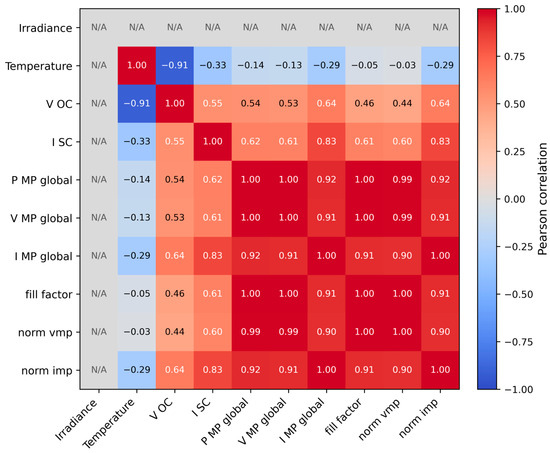
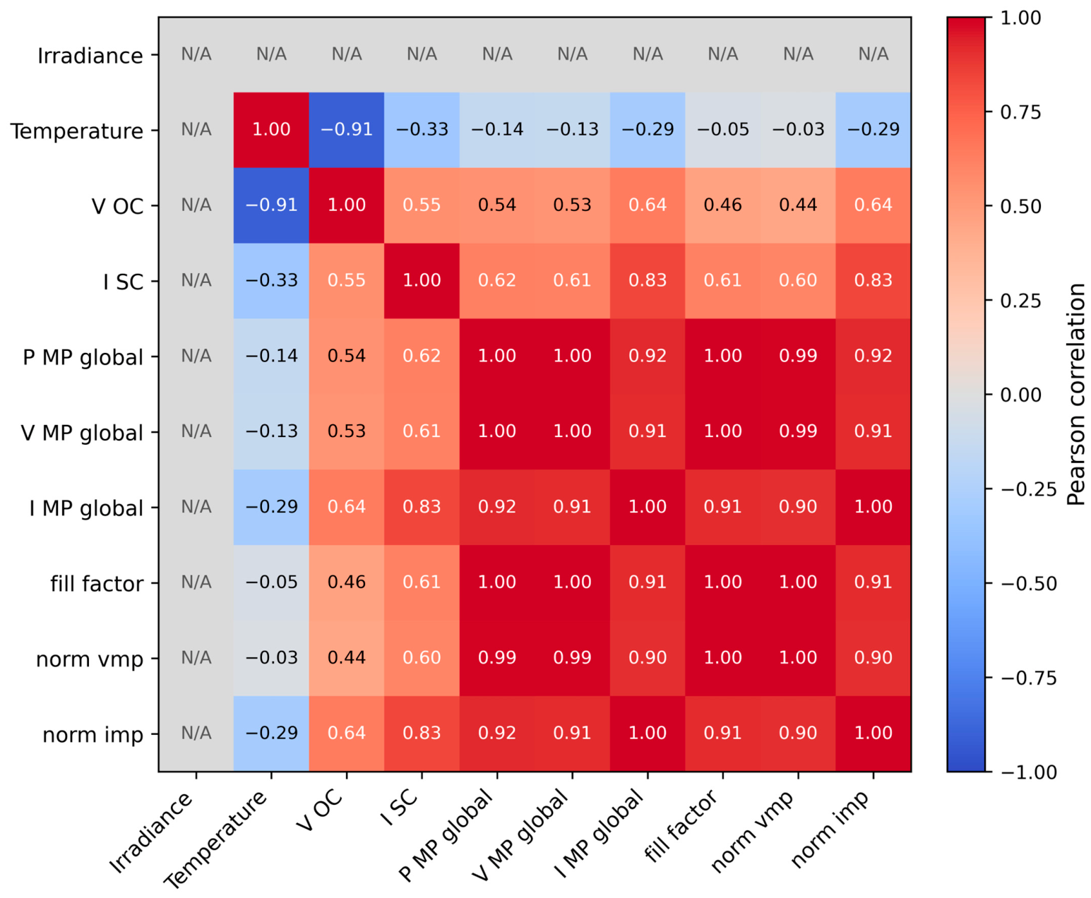
The 10-feature core representation contains irradiance, temperature, open-circuit voltage, short-circuit current, global MPP power, voltage and current, fill factor, and normalized MPP coordinates. Figure 7 shows strong correlations among the MPP-derived quantities, which is physically expected because several descriptors encode related aspects of the same operating point. The purpose of the feature set is therefore not statistical independence, but complementary and interpretable description of PV operating state.
Figure 7.
Pearson correlation matrix for the 10-feature core set; correlation coefficients are dimensionless.
The 10-feature core representation combines environmental context with supplied and reconstructed MPP landmarks. Figure 7 shows the dimensionless Pearson correlations among standardized core features. Strong dependence among MPP-derived quantities is physically expected because P_MP = V_MP I_MP and FF = P_MP/(V_OC I_SC). Coefficients are therefore interpreted as predictive associations among correlated descriptors, not independent causal effects. Principal component analysis provides an unsupervised view of class structure before classifier fitting. Figure 8 shows ordered separation among the shading classes in the first two principal components, while temperature-related variation remains within the class trajectories. This confirms that much of the diagnostic separability originates in the engineered electrical representation rather than classifier complexity alone. Even though some features are related by physical principles, the purpose of the feature set is not just to provide a set of independent variables. Instead, these variables offer complementary ways to describe the electrical operating conditions. The global MPP variables describe the actual electrical behaviour, whereas the fill factor and normalized coordinates provide dimensionless descriptions that help distinguish changes caused by shading from those due to operating conditions. Principal component analysis in Figure 8 shows ordered within-source separation among nominal severity classes. The horizontal and vertical axes are standardized principal component scores and are dimensionless. The plot describes the controlled cohort only and is not external-validation evidence. The PCA projection should not be interpreted as external evidence of generalization; it describes structure within the controlled cohort. Its value is to show why compact linear models can perform competitively when the dominant shading effects are already expressed in the selected physical descriptors.
Figure 8.
Two-component PCA projection of standardized core features. PC1 and PC2 scores are dimensionless; the unintended horizontal paragraph rule present in the earlier version has been removed.
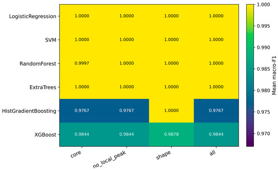
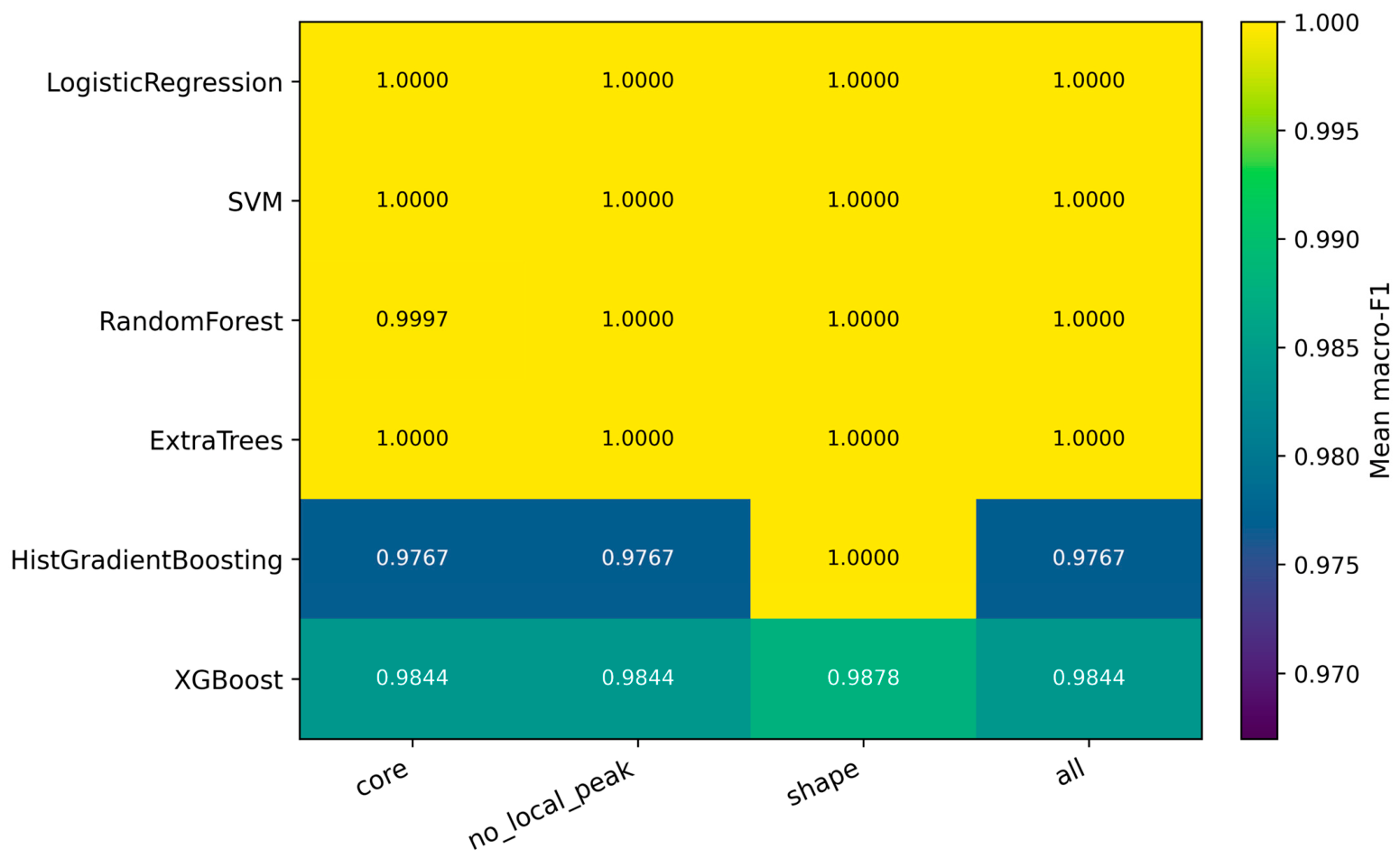
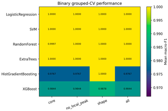
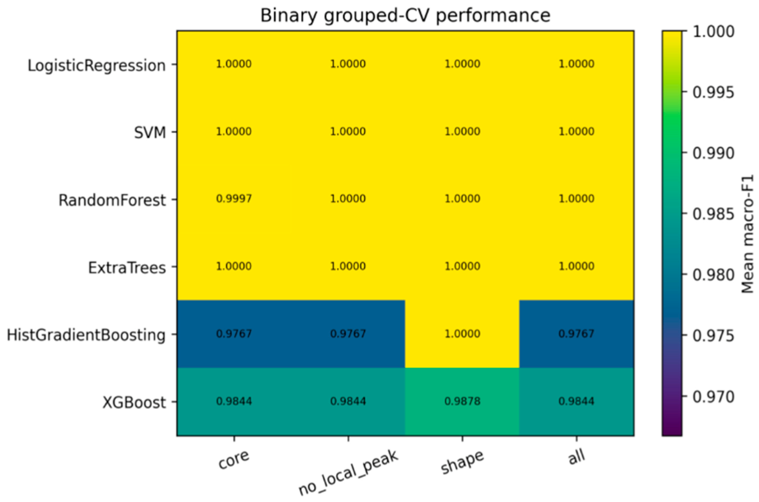
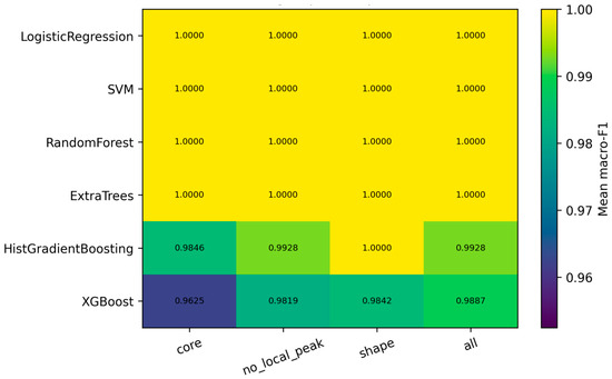
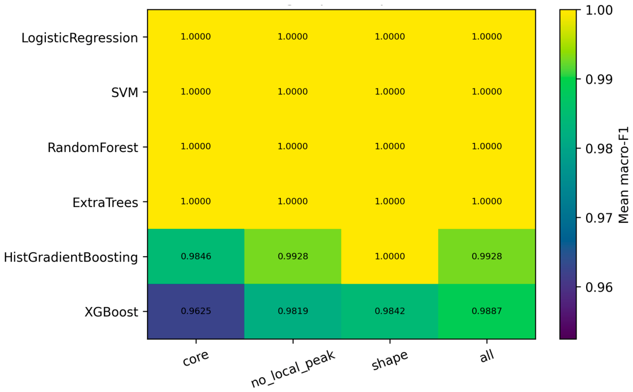
The fixed benchmark compares six classifiers across four predefined feature sets for both binary detection and six-class severity diagnosis. All configurations are evaluated over 30 repeated temperature-grouped five-fold splits. Figure 9 and Figure 10 summarize mean macro-F1 for the binary and multiclass tasks, respectively. Figure 9 reports mean binary macro-F1 and Figure 10 reports mean six-class macro-F1; both are based on the mean dimensionless macro-F1 across 30 repeated temperature-grouped five-fold validations for the binary and six-class tasks, respectively.
Figure 9.
Mean binary macro-F1 across classifiers and feature sets.
Figure 10.
Mean multiclass macro-F1 across classifiers and feature sets.
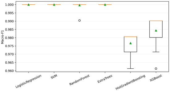
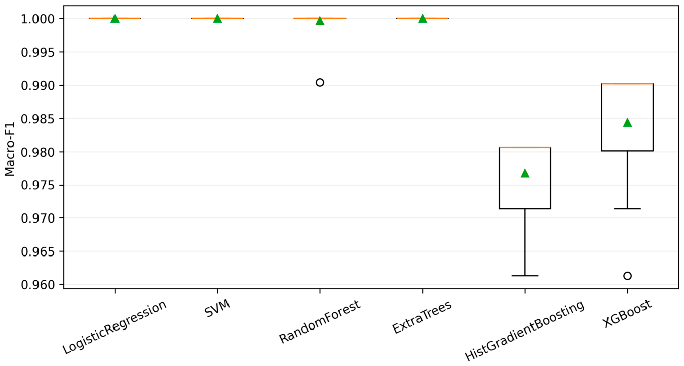
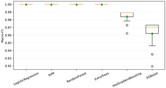
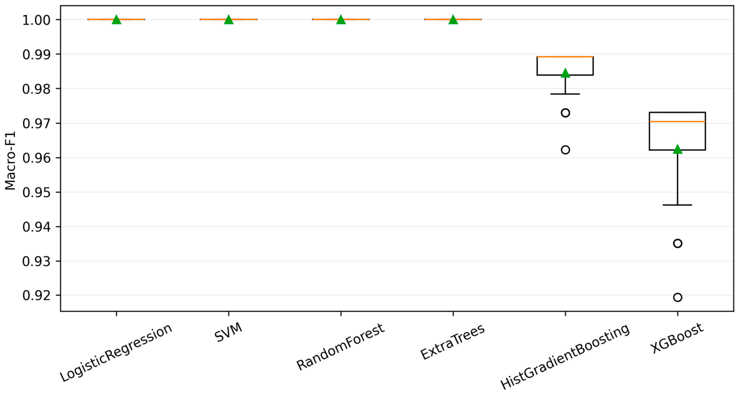
The core representation is sufficient for perfect or near-perfect grouped classification by several models. With core features, LR, RBF-SVM, and Extra Trees achieve mean binary macro-F1 = 1.000; for six-class diagnosis, LR, RBF-SVM, Random Forest, and Extra Trees achieve 1.000. Added feature complexity offers no consistent gain. Importantly, the single normalized-MPP-voltage LR baseline also achieves macro-F1 = 1.000 for both tasks, while the shallow tree reaches 1.000 for binary and 0.400 for six-class diagnosis (Appendix A.8). The source labels are therefore strongly separable and partly rule-like. Figure 11 shows the binary repeated distributions, and Figure 12 shows the six-class repeated distributions for the repeated core-feature distributions.
Figure 11.
Thirty-repeat binary macro-F1 distributions for core features. Green triangles indicate the mean, orange horizontal lines indicate the median, open circles indicate outliers, boxes represent the interquartile range, and whiskers extend to 1.5 times the interquartile range.
Figure 12.
Thirty-repeat multiclass macro-F1 distributions for core features. Green triangles indicate the mean, orange horizontal lines indicate the median, open circles indicate outliers, boxes represent the interquartile range, and whiskers extend to 1.5 times the interquartile range.
These clean results are stable across the available temperature groups, but they do not show transfer across modules, irradiances, shadow geometries, instruments, or mixed faults. Model selection therefore prioritizes parsimony and robustness rather than claiming that higher algorithmic complexity created the separation.
4.3. Statistical and Inferential Comparison
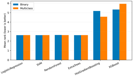
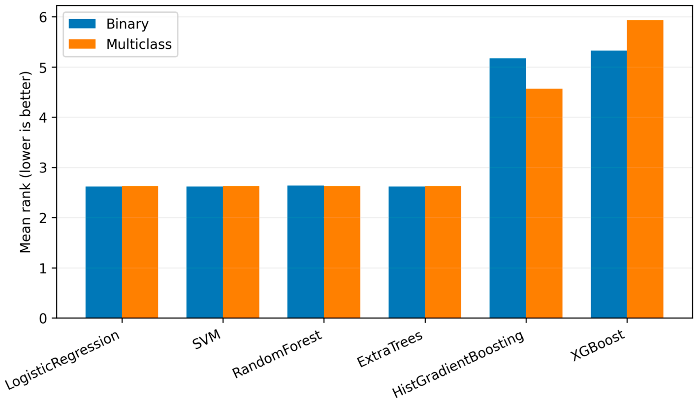
Figure 13 reports average classifier ranks. The repeated grouped evaluations support comparative stability. Because repetitions reuse the same 186 records, the Friedman and Wilcoxon–Holm results are interpreted as exploratory paired-resampling evidence. Temperature-group bootstrap intervals provide the principal uncertainty statement: nested macro-F1 is 1.000 with 95% CI 1.000–1.000 for both tasks (Appendix A.5).
Figure 13.
Average classifier ranks across the four feature sets for binary and multiclass diagnosis.
The inferential results show that identical headline macro-F1 values do not imply identical model behaviour across all paired repetitions or probability outputs. Repeated grouped validation and corrected non-parametric tests therefore provide stronger comparative evidence than a single train–test split.
4.4. Nested Grouped Validation and Final Model Performance
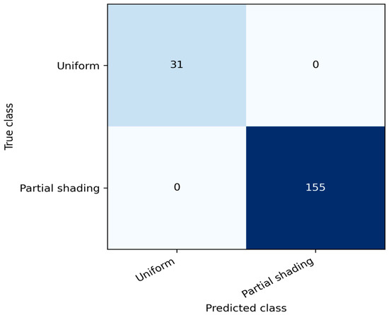
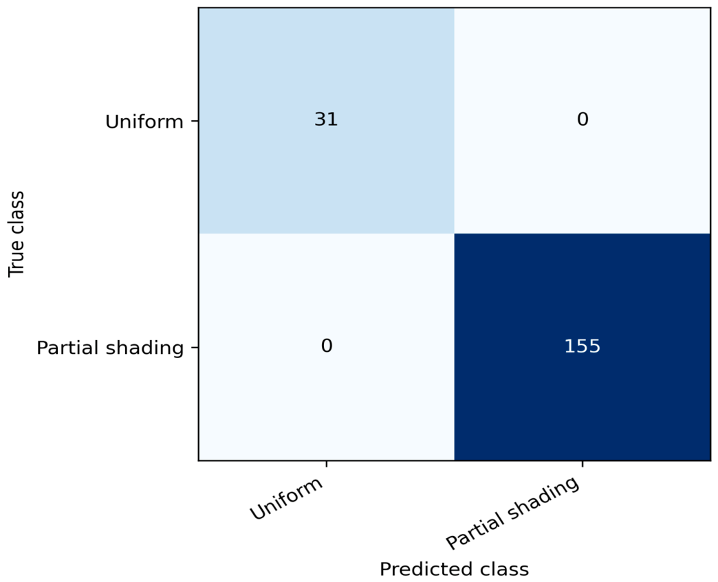
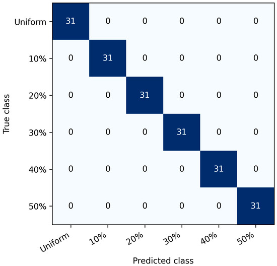
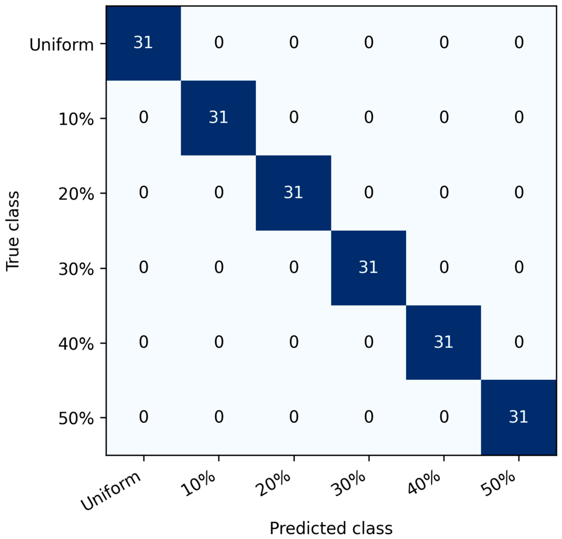
The 10-feature LR model is confirmed by five-outer/four-inner temperature-grouped validation. Both tasks produce perfect out-of-fold assignments. Binary log loss is 0.00002391 and six-class log loss is 0.00032779. Figure 14 shows the binary confusion matrix and Figure 15 shows the six-class confusion matrix; both represent the confusion matrices, while Appendix A.5 reports group-bootstrap intervals and class-wise disturbance results.
Figure 14.
Binary nested grouped-CV confusion matrix.
Figure 15.
Multiclass nested grouped-CV confusion matrix.
Every class has precision, recall, and F1 = 1.000 in the clean nested evaluation. This establishes strong internal transfer across the represented temperatures only. It does not establish field accuracy.
4.5. Final Hyperparameter Search and Model Selection
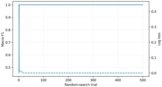
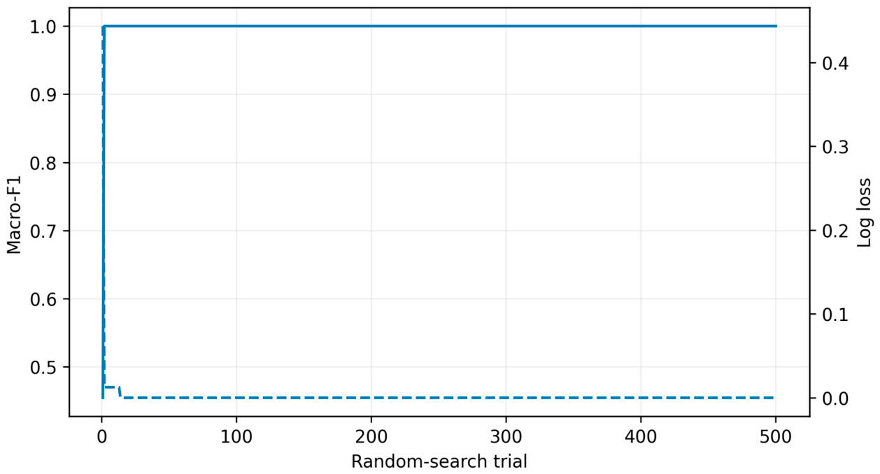
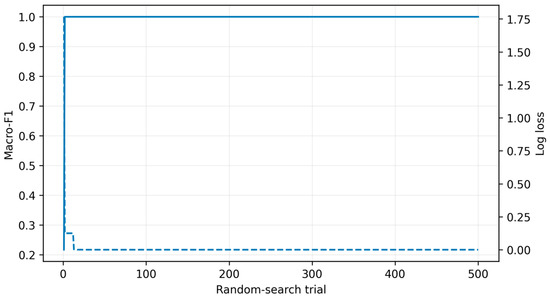
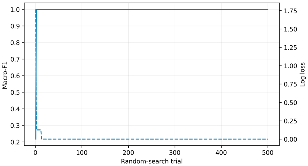
The full-data grouped searches select high-C logistic models under clean measurements. The binary search selects trial 419 with C = 7610.7929, while the multiclass search selects trial 64 with C = 7970.2028. Both achieve grouped macro-F1 = 1.000 with balanced class weights, an intercept, and the L-BFGS solver. Figure 16 shows the binary search trajectory and Figure 17 shows the six-class search trajectory; both depict the respective search convergence.
Figure 16.
Binary full-data 500-trial grouped-search convergence.
Figure 17.
Multiclass full-data 500-trial grouped-search convergence.
The final clean-data grouped searches select high-C LR models: C = 7610.7929 for binary detection and C = 7970.2028 for six-class diagnosis. Figure 16 shows the binary search trajectory, and Figure 17 shows the six-class search trajectory; both depict the search trajectories. Large C values indicate weak regularization and very steep boundaries in a nearly separable feature space.
Because many candidates tie at macro-F1 = 1.000, log loss favours very confident boundaries. The disturbance analysis demonstrates that this clean-data confidence is not equivalent to operational robustness.
4.6. Explainability and Feature-Importance Analysis
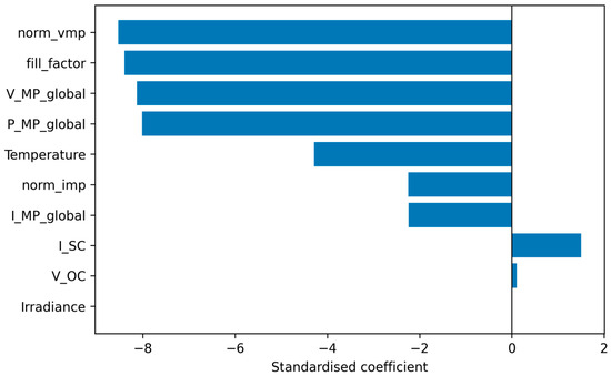
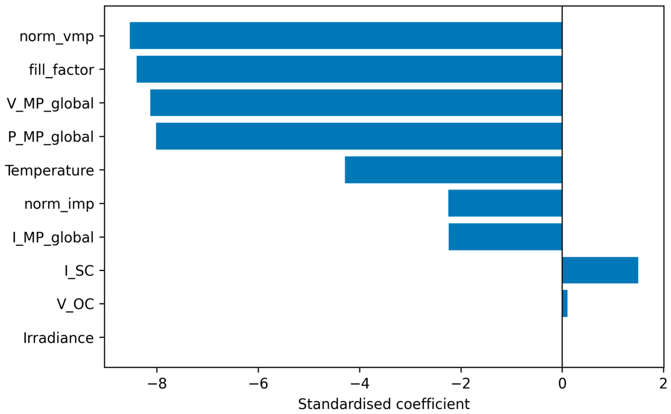
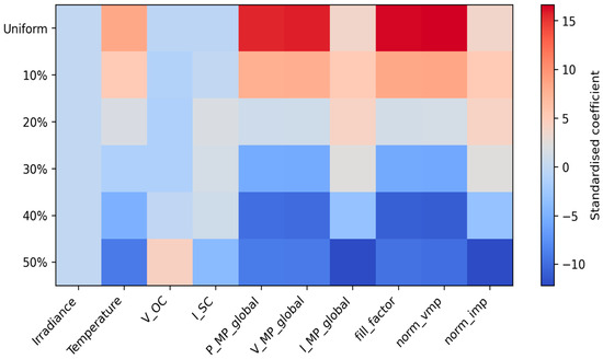
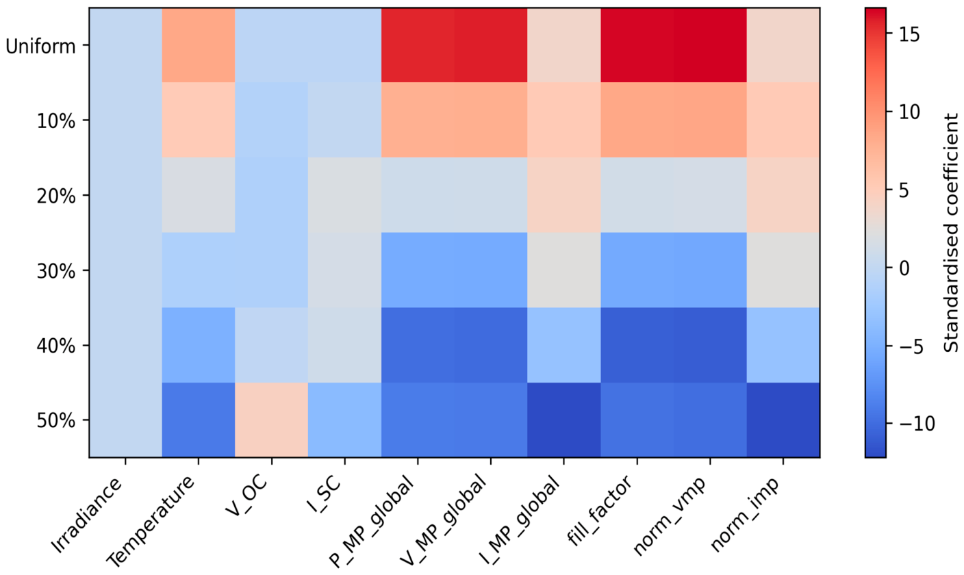
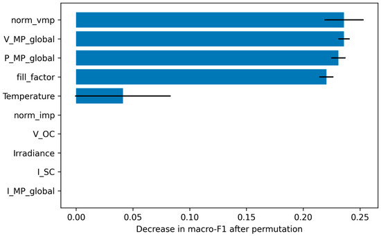
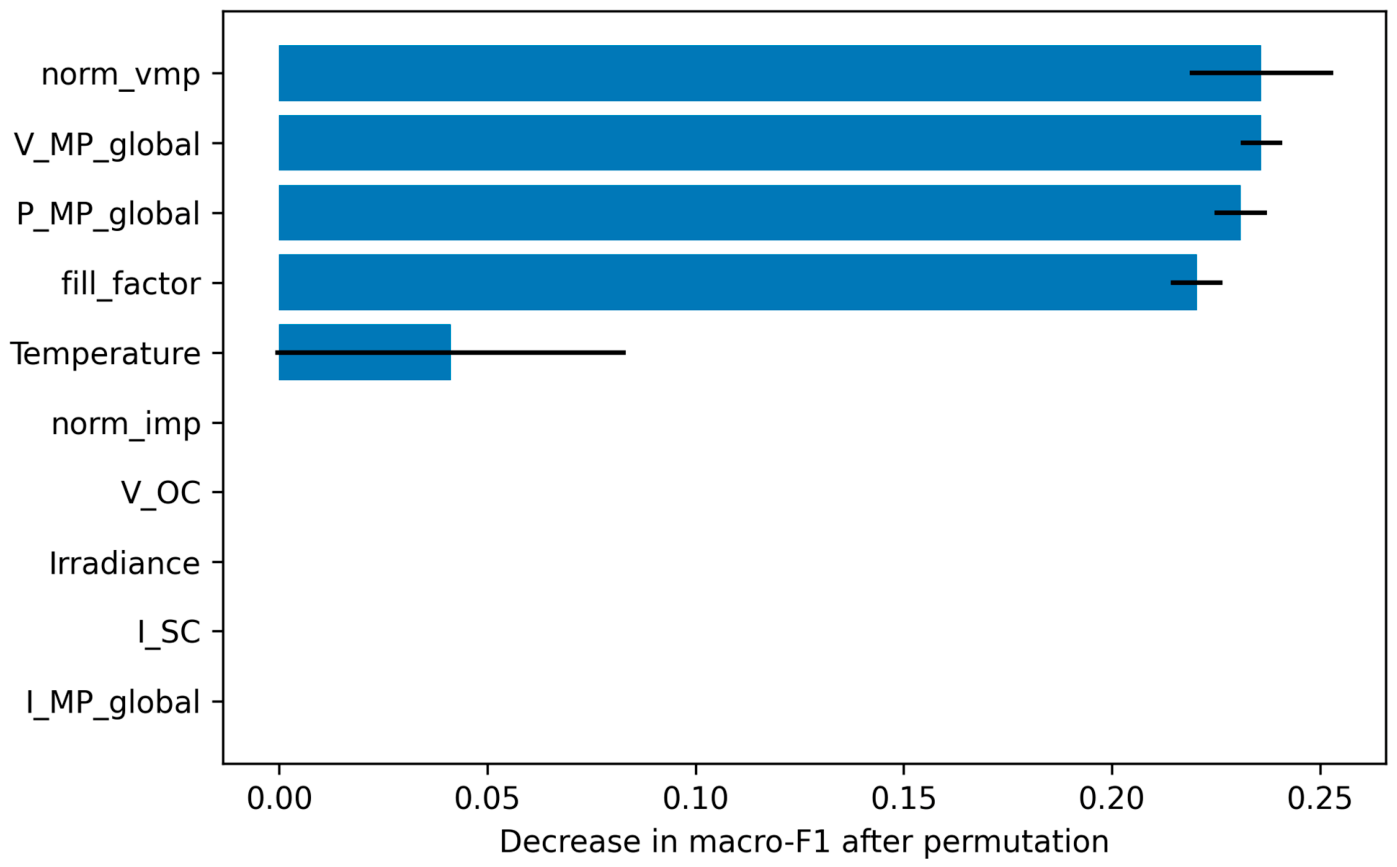
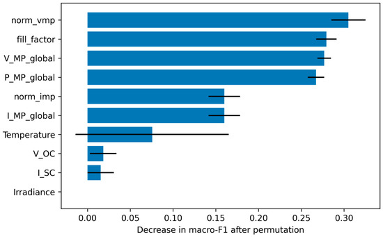
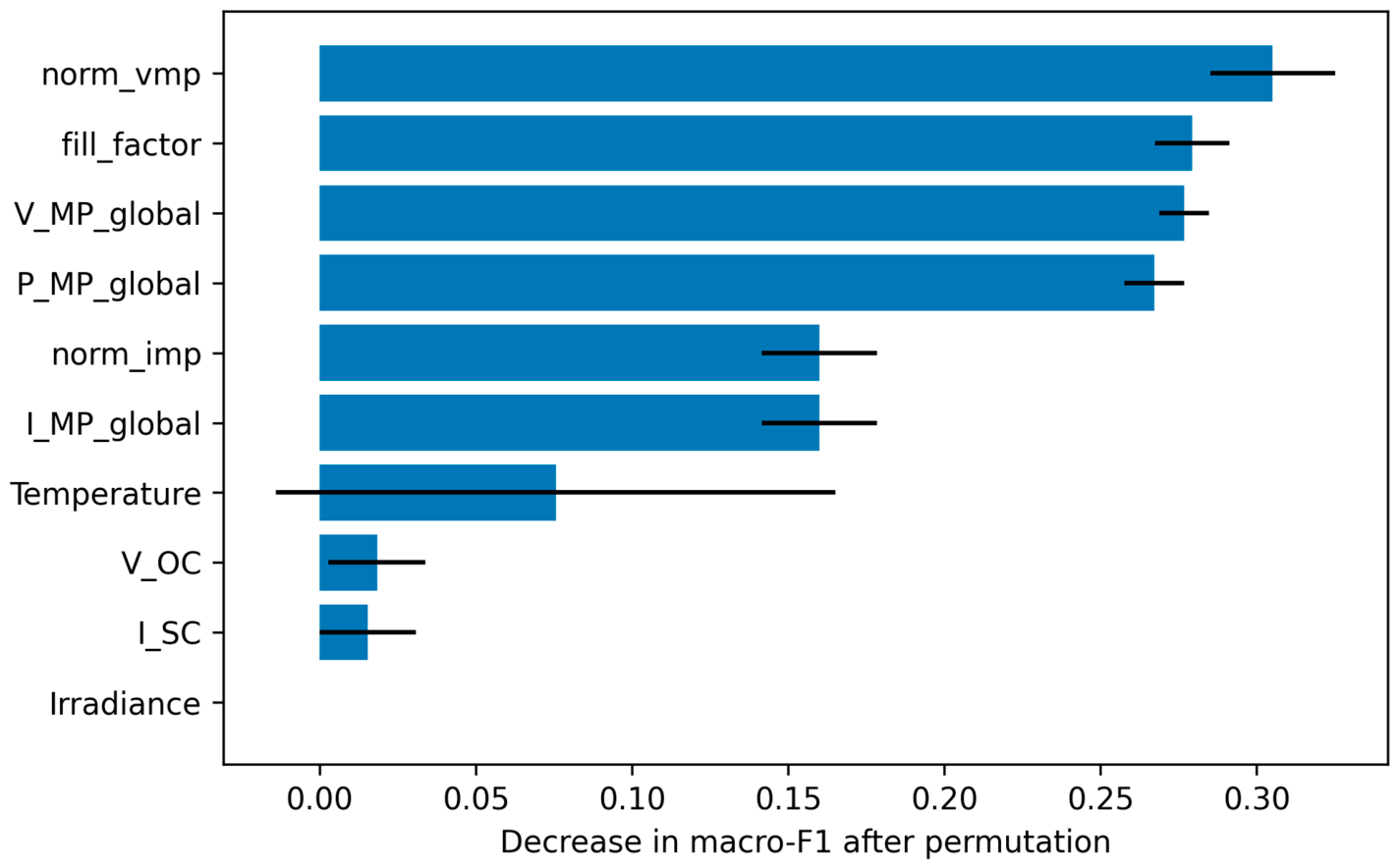
Explainability is evaluated with standardized coefficients and nested permutation importance. For binary detection, normalized MPP voltage, V_MP, P_MP, and FF have importance values of 0.236, 0.236, 0.231, and 0.220. For six-class diagnosis, normalized MPP voltage is highest at 0.305, followed by FF (0.279), V_MP (0.277), and P_MP (0.267). Figure 18 shows binary coefficients, Figure 19 shows class-specific multiclass coefficients, Figure 20 shows binary permutation importance, and Figure 21 shows multiclass permutation importance.
Figure 18.
Standardized coefficients of the final binary logistic-regression model.
Figure 19.
Class-specific standardized coefficients of the multiclass logistic-regression model.
Figure 20.
Nested outer-fold permutation importance for binary detection.
Figure 21.
Nested outer-fold permutation importance for multiclass diagnosis.
The dominant features are physically coherent. Partial shading reduces the effective photocurrent of shaded cells and may activate bypass paths, deforming the I–V knee and shifting the global operating point. V_MP/V_OC records displacement relative to the open-circuit endpoint; FF measures contraction of the usable power rectangle; V_MP locates the selected global peak; and P_MP captures the resulting available-power reduction. Their joint importance is expected, but their algebraic dependence means they should not be treated as independent causal mechanisms.
4.7. Multi-Mechanism Sensor-Error Robustness and Class Confusion
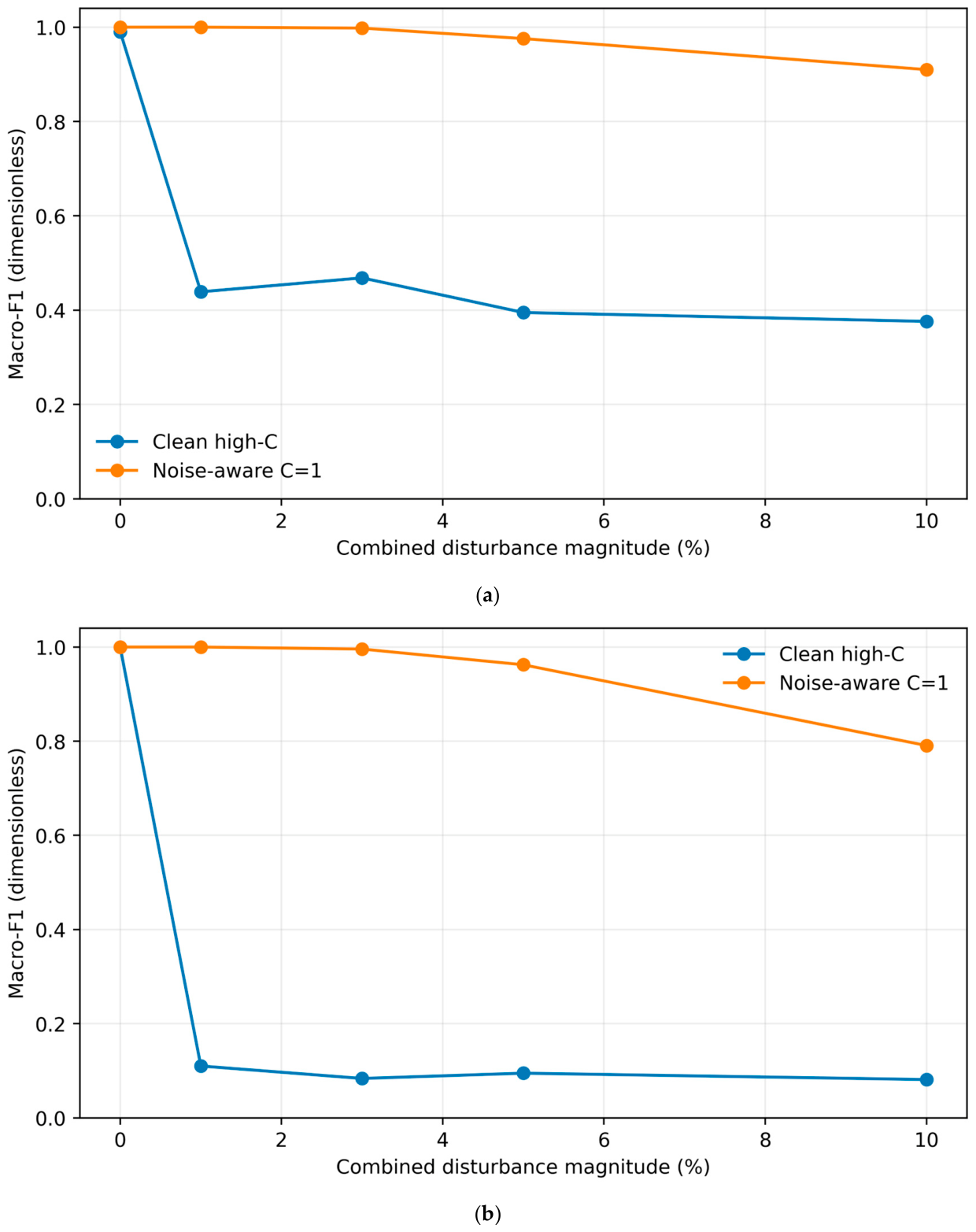
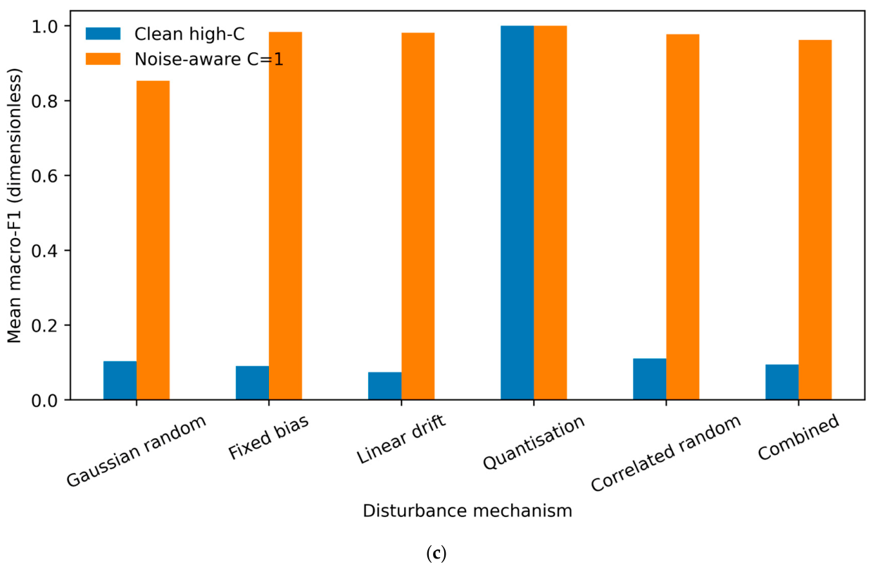
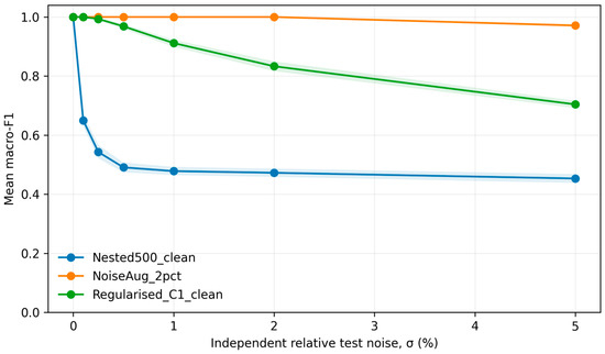
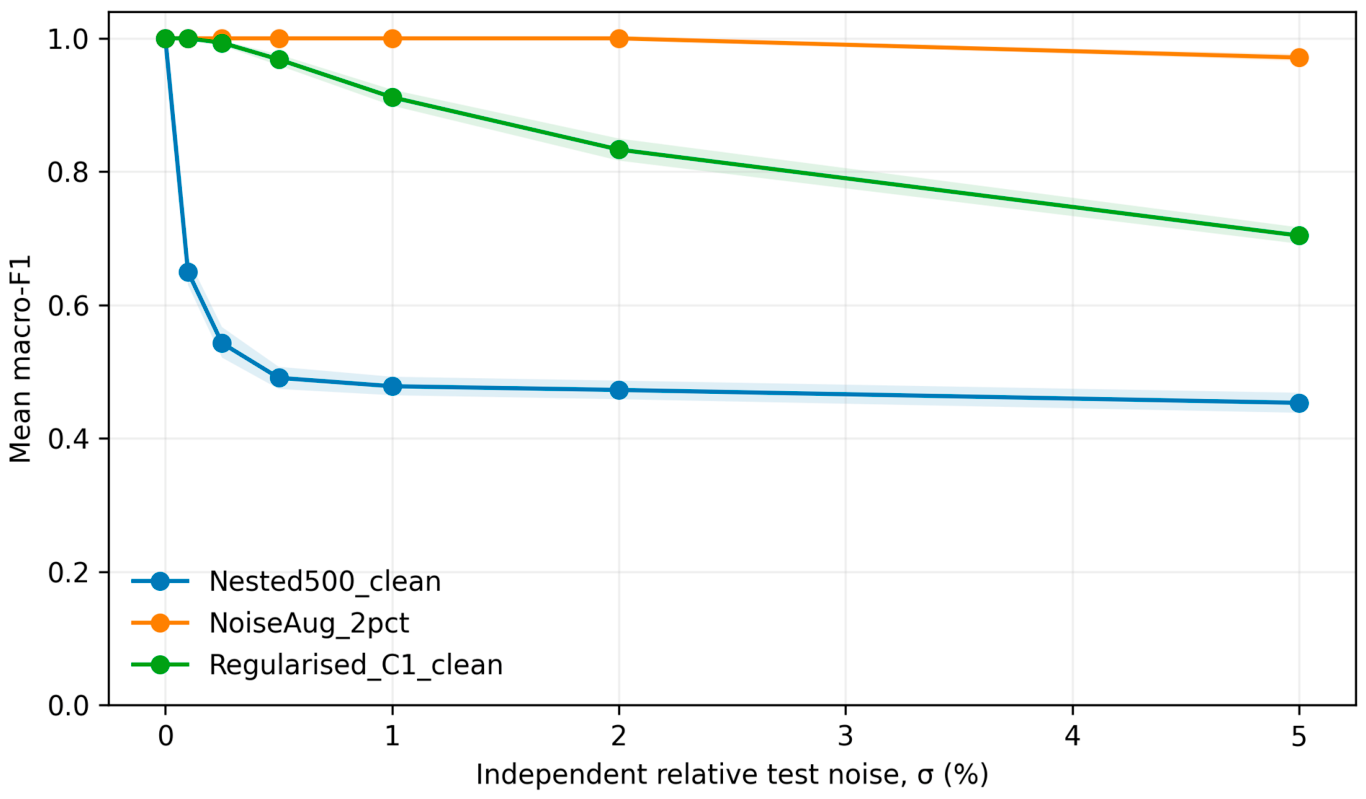
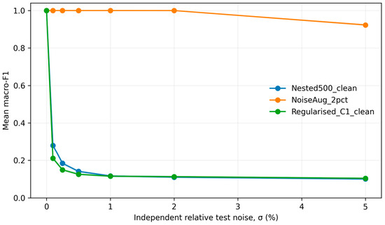
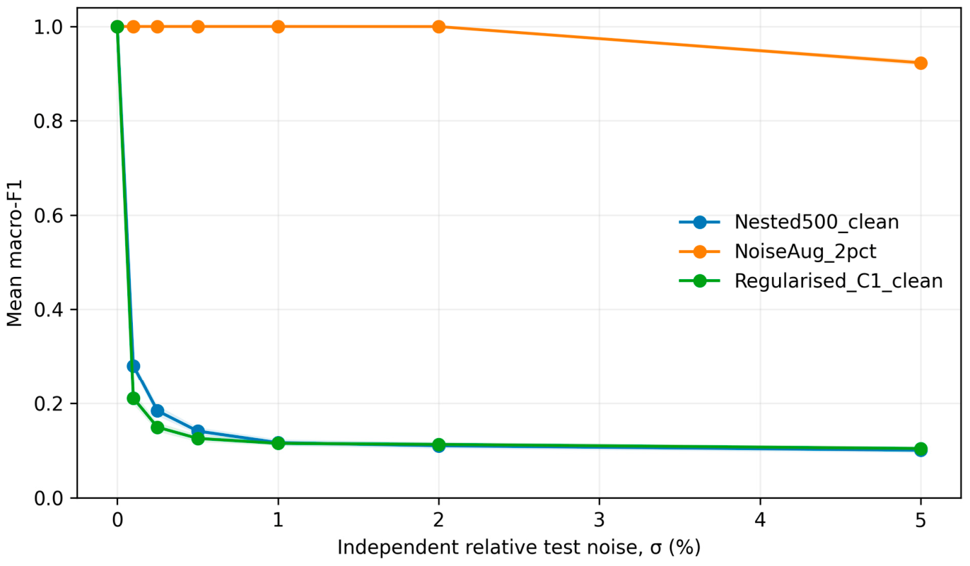
The original Gaussian perturbation experiment showed that the clean high-C model falls to macro-F1 = 0.453 for binary and 0.101 for six-class diagnosis at 5% relative noise, whereas noise-aware training retained 0.971 and 0.923. The expanded analysis confirms that the vulnerability is not confined to white noise. At 5% combined Gaussian, bias, drift, and quantisation disturbance, clean high-C mean macro-F1 is 0.395 ± 0.040 for binary and 0.095 ± 0.019 for six-class diagnosis; the noise-aware C = 1 model retains 0.976 ± 0.012 and 0.962 ± 0.022, respectively. Figure 22 retains the original binary trajectory and Figure 23 retains the original six-class trajectory; Appendix A Figure A1 reports the combined-noise extension, and Appendix A Table A3 gives the full 5% mechanism comparison.
Figure 22.
Binary mean macro-F1 under 0–5% independent relative sensor noise.
Figure 23.
Multiclass mean macro-F1 under 0–5% independent relative sensor noise.
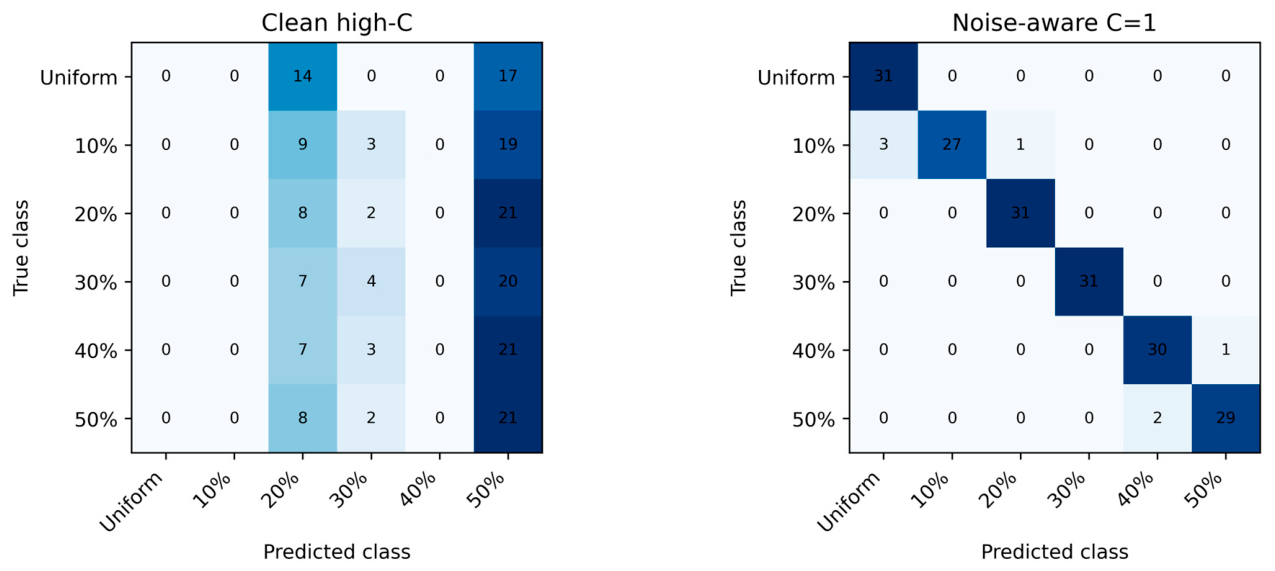
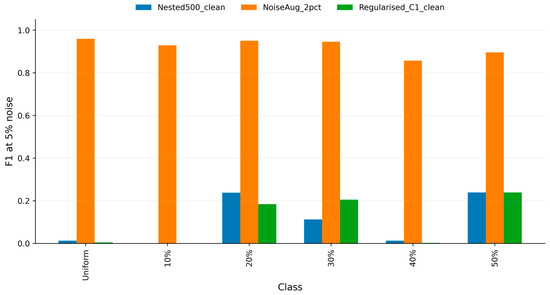
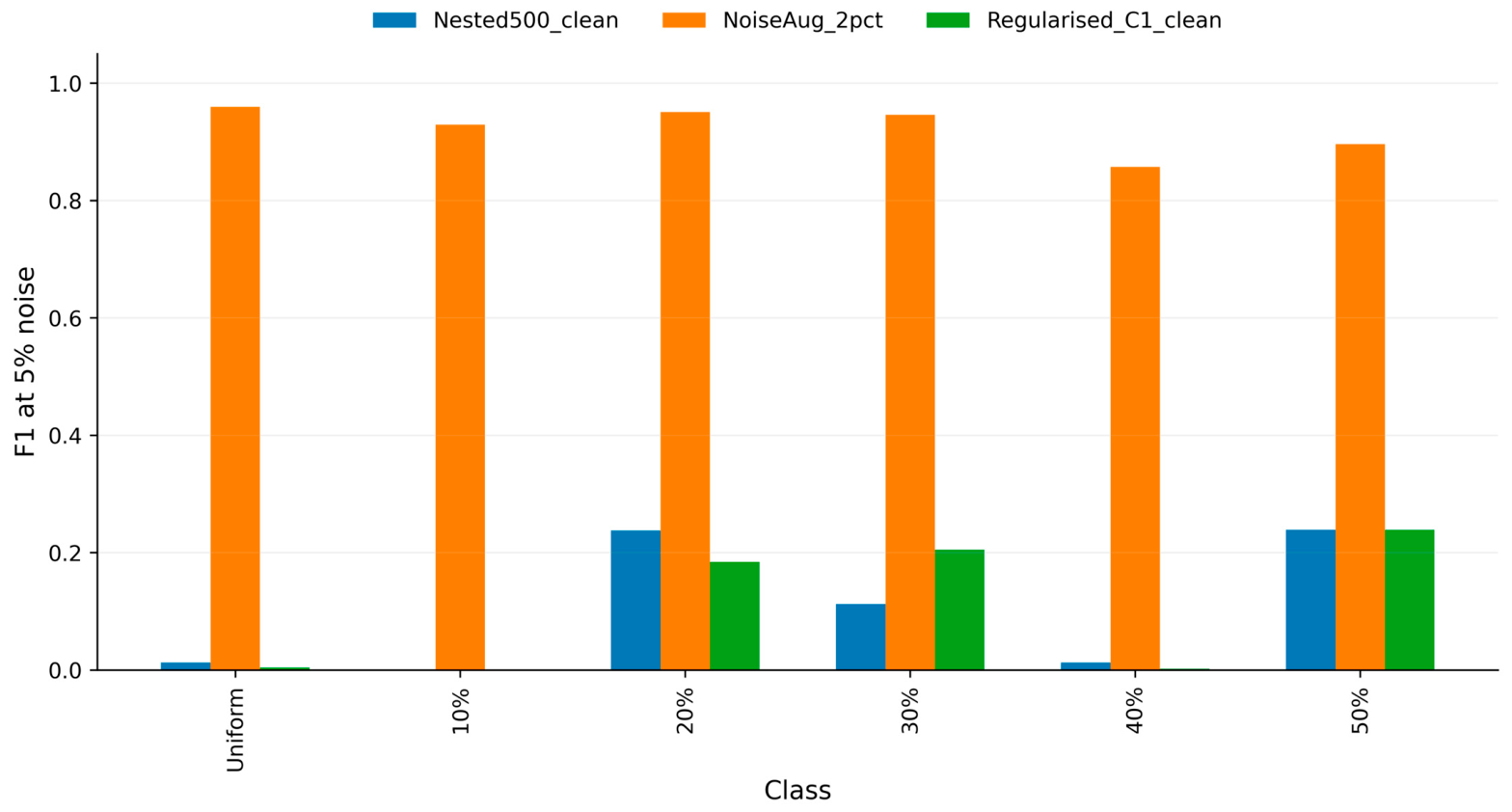
Figure 24 shows class-wise behaviour at 5% test noise; the corresponding 5% combined-disturbance confusion matrices are provided in Appendix A.5. Under combined error, the clean high-C multiclass model has F1 = 0 for Uniform, 10%, and 40% and remains weak for 20%, 30%, and 50%. Noise-aware training raises class-wise F1 to 0.931–1.000. The result supports uncertainty-aware training within this source domain, but not universal robustness to unobserved instruments or environments.
Figure 24.
Class-wise multiclass F1 at 5% test noise for the three deployment variants.
4.8. Computational Profile and Reproducibility
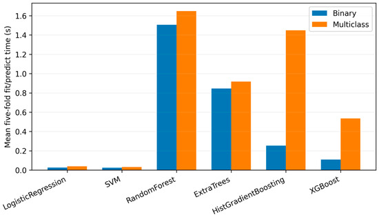
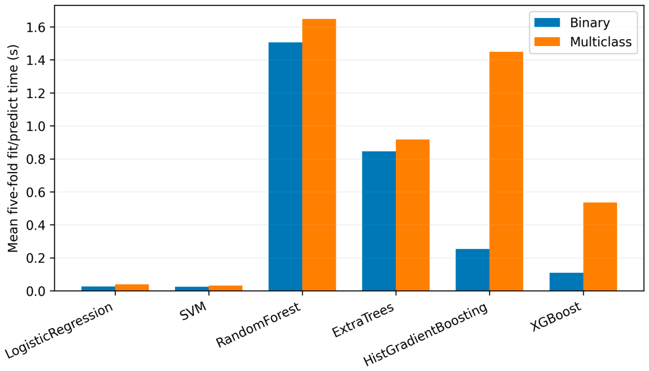
The principal benchmark contains 1440 repeat-level evaluations and 267,840 out-of-fold predictions. Nested confirmation evaluates 500 candidates in each inner search, and the final searches add 1000 candidate evaluations. The revision package adds parsimonious baselines, group-bootstrap confidence intervals, six disturbance mechanisms across multiple magnitudes, class-level confusion matrices, and a cross-irradiance negative control. Figure 25 reports mean five-fold fit-and-predict runtime; time is expressed in seconds.
Figure 25.
Mean five-fold fit-and-predict runtime by classifier and task, averaged over feature sets.
All stochastic components are seeded. The compact LR model has low fitting cost and direct interpretability; nevertheless, reproducibility of the computational result does not remove the need for independent empirical validation.
4.9. Practical Acquisition, Cross-Irradiance Check, and Economic Implications
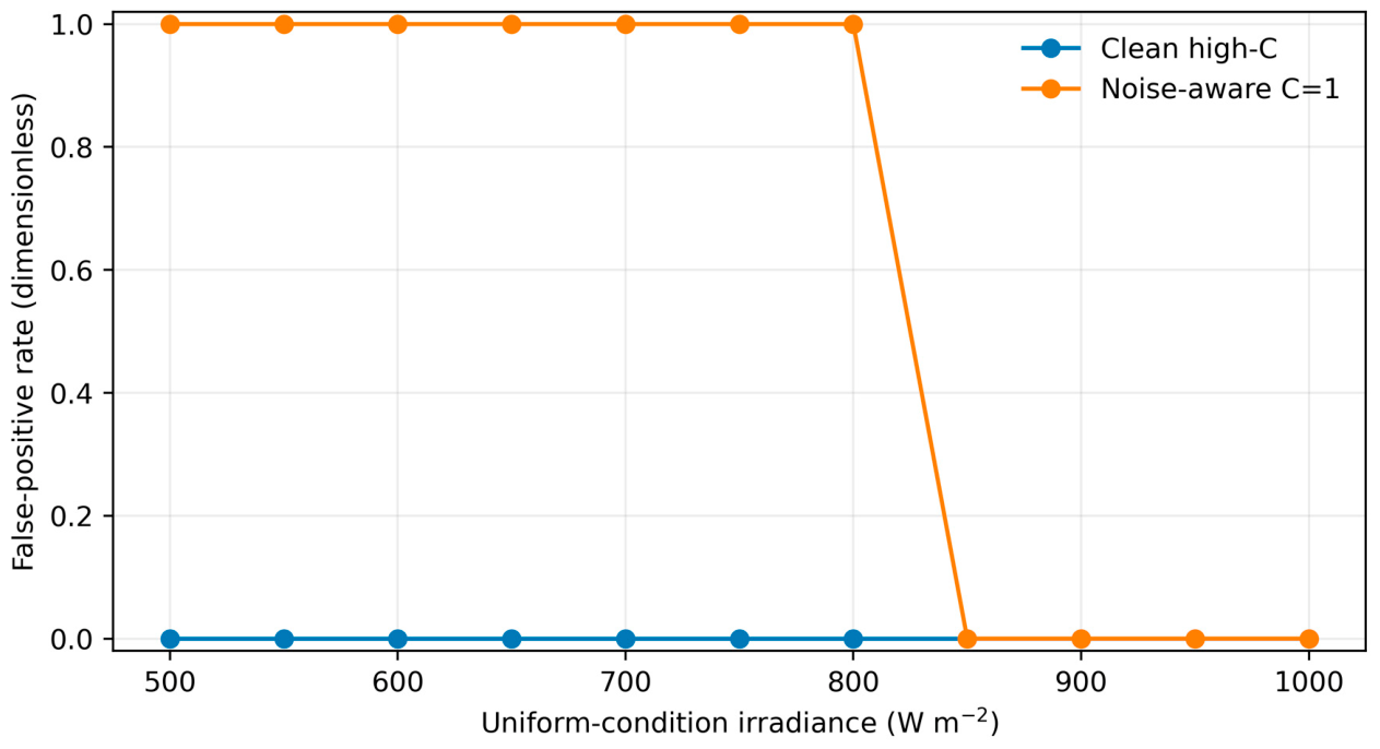
Operational use requires an I–V acquisition path. Portable tracers and programmable electronic loads can sweep the array away from its MPP and may briefly interrupt energy production; switched-converter or inverter-integrated sweeps can reduce intervention but require compatible power electronics, synchronized irradiance and temperature measurements, and appropriate safety controls. The limited Uniform-only negative control across 500–1000 W m−2 produced no false positives for the clean high-C model, but the noise-aware C = 1 model classified all Uniform records below 850 W m−2 as shaded (Appendix A Table A4 and Figure A2). This exposes irradiance-domain shift and confirms that lower-irradiance training data are required before online deployment. Scan-related opportunity cost depends on array rating, sweep duration, frequency, irradiance, and electricity value. As an illustrative upper-bound calculation, a 100 kW array subjected to a 1 s full-power-equivalent scan four times per day would forgo about 40.56 kWh year−1, valued at USD 4.06–12.17 year−1 at USD 0.10–0.30 kWh−1 (Appendix A.7). This excludes tracer capital, labour, communications, downtime, and avoided-failure benefits and is not a life-cycle economic assessment.
4.10. Limitations
The study has six principal limitations. First, the source is model-generated, and the primary cohort is small and controlled: 186 records, one irradiance, one underlying PV representation, and 31 temperatures. Second, the nominal severity labels are supplied by the dataset creators, but no independent spatial shadow-pattern identifier is released; same-severity/different-pattern validation is therefore impossible without fabricating metadata. Third, one normalized voltage feature already separates the classes, so perfect clean metrics partly reflect the source-generation structure. Fourth, the available lower-irradiance data support only a Uniform negative control, not matched cross-irradiance severity evaluation. Fifth, the disturbance mechanisms are controlled stress tests and do not constitute a certified uncertainty model for a specific tracer, inverter, or sensor chain. Sixth, repeated cross-validation reuses observations, and its paired tests are exploratory. External measured validation must therefore span module technologies, array topologies, irradiance, shading geometry, ageing, soiling, mixed faults, acquisition systems, and sites.
5. Conclusions
This study presents a noise-robust, feature-based framework for photovoltaic partial-shading diagnosis using a public model-generated I–V benchmark. The verified analysis uses 186 balanced curves, six nominal operating states, 37 predictors in four predefined representations, six classifiers, 30 repeated temperature-grouped validations, nested grouped confirmation, parsimonious baselines, explanation, and multi-mechanism uncertainty tests. Clean nested performance is perfect for both tasks, but a single normalized MPP-voltage predictor also reaches macro-F1 = 1.000, indicating low-dimensional and partly rule-driven separability. The principal scientific result is therefore the contrast between clean discrimination and deployment sensitivity. Under 5% combined disturbance, the clean high-C model falls to macro-F1 = 0.395 for binary and 0.095 for six-class diagnosis, whereas noise-aware training retains 0.976 and 0.962. Dominant features are physically consistent with MPP displacement and contraction of usable power, but cross-irradiance negative-control failures show that robustness within one source domain does not establish field transfer. The framework is reproducible and useful as a controlled benchmark; operational adoption requires external measured data, multiple irradiances, independent shadow patterns, multiple modules and arrays, instrument-specific uncertainty characterization, and prospective acquisition/economic evaluation.
Author Contributions
Conceptualization, R.D.P. and B.A.T.; methodology, R.D.P.; software, R.D.P.; validation, R.D.P. and B.A.T.; formal analysis, R.D.P.; investigation, R.D.P.; resources, B.A.T.; data curation, R.D.P.; writing—original draft preparation, R.D.P.; writing—review and editing, R.D.P. and B.A.T.; visualization, R.D.P.; supervision, B.A.T.; project administration, B.A.T. All authors have read and agreed to the published version of the manuscript.
Funding
This research received no external funding.
Institutional Review Board Statement
Not applicable.
Informed Consent Statement
Not applicable.
Data Availability Statement
The source is a public model-generated dataset available in Mendeley Data, Version 1, at https://doi.org/10.17632/z93gzbptf7.1. The associated generation study is cited as Reference [32]. The revision package contains the analysis code, derived Tables, and Figures used for the additional robustness and audit analyses.
Acknowledgments
The authors acknowledge the Department of Electrical and Electronic Engineering Technology, University of Johannesburg, for institutional support.
Conflicts of Interest
The authors declare no conflicts of interest.
Abbreviations and Symbols
The following abbreviations and symbols are used in this manuscript:
| AI | Artificial intelligence |
| ML | Machine learning |
| PV | Photovoltaic |
| I–V | Current-voltage |
| P–V | Power-voltage |
| MPP | Maximum power point |
| VOC | Open-circuit voltage |
| ISC | Short-circuit current |
| V_MP | Voltage at maximum power point |
| I_MP | Current at maximum power point |
| P_MP | Power at maximum power point |
| FF | Fill factor |
| LR | Logistic regression |
| RBF-SVM | Radial basis function support-vector machine |
| RF | Random forest |
| XGBoost | Extreme Gradient Boosting |
| XAI | Explainable artificial intelligence |
| MAE | Mean absolute error |
| RMSE | Root mean square error |
| MaxAE | Maximum absolute error |
| MCC | Matthews correlation coefficient |
| ROC | Receiver operating characteristic |
| AUC | Area under the curve |
| ROC-AUC | Receiver operating characteristic area under the curve |
| CV | Cross-validation |
| CI | Confidence interval |
| SG | Savitzky–Golay |
| X | Input feature matrix |
| y | Target vector |
| n | Number of observations |
| p | Number of predictors |
| K | Number of classes |
| C | Inverse regularization strength |
| κ | Cohen’s kappa |
| μ | Feature mean |
| σ | Feature standard deviation or sensor-noise level, as defined by context |
| ε | Random perturbation term |
| r | Pearson correlation coefficient |
Appendix A. Reproducibility, Robustness, and Deployment Evidence
Appendix A.1. Dataset Provenance
Appendix A Table A1 records all source-generation details that could be verified and explicitly identifies unavailable metadata. It is cited in Section 2.1.
Table A1.
Verified public-dataset provenance and reproducibility boundary.
Appendix A.2. Complete Predictor Inventory
Appendix A Table A2 is the definitive 37-predictor inventory cited in Section 2.2 and Section 3.3. Units marked dimensionless are ratios or standardized geometric descriptors.
Table A2.
Complete verified feature inventory with extraction procedure, unit, and physical interpretation.
Appendix A.3. Disturbance Mechanisms and Sensitivity
Table A3a defines the six controlled error mechanisms. Table A3b reports the 5% results cited in Section 4.8; Figure A1a shows the binary combined-error trajectory, Figure A1b shows the six-class combined-error trajectory, and Figure A1c compares 5% disturbance mechanisms. Macro-F1 and balanced accuracy are dimensionless.
Table A3.
(a). Controlled sensor-error stress-test mechanisms. (b). Performance under 5% disturbance by error mechanism.
Figure A1.
(a). Binary macro-F1 under combined sensor disturbance; noise magnitude is expressed as a percentage and macro-F1 is dimensionless. (b). Six-class macro-F1 under combined sensor disturbance; noise magnitude is expressed as a percentage and macro-F1 is dimensionless. (c). Six-class macro-F1 under a 5% disturbance mechanism. All performance values are dimensionless.
Appendix A.4. Uniform Cross-Irradiance Negative Control
Table A4 and Figure A2 are cited in Section 4.10. They test false positives on Uniform records only and do not constitute cross-irradiance severity validation.
Table A4.
Uniform-only cross-irradiance false-positive check.
Figure A2.
False-positive rate for Uniform records across irradiance; irradiance is in W m−2 and false-positive rate is dimensionless.
Appendix A.5. Confidence Intervals and Class-Wise Performance
Table A5a,b and Figure A3 are cited in Section 4.5 and Section 4.8. The bootstrap unit is the temperature group rather than the individual row.
Table A5.
(a). Temperature-group bootstrap confidence intervals for nested grouped macro-F1. (b). Class-wise performance at 5% combined disturbance.
Figure A3.
Six-class confusion matrices at 5% combined disturbance. Cell values are counts of model-generated I–V records.
Appendix A.6. Symbol and Unit Register
Table A6 is cited at the first equation block and standardizes MPP notation as V_MP, I_MP, and P_MP throughout.
Table A6.
Mathematical symbols, definitions, and SI units or dimensions.
Appendix A.7. Illustrative Scan-Interruption Sensitivity
Table A7 is cited in Section 4.10. It reports full-power-equivalent opportunity cost only and excludes equipment, labour, communications, downtime, and avoided-failure benefits.
Table A7.
Illustrative annual opportunity cost of I–V scan interruption.
Appendix A.8. Parsimonious Baselines and Feature Discriminability
Table A8a reports the grouped parsimonious baselines cited in Section 4.3. Table A8b shows that normalized MPP voltage has non-overlapping class ranges in the controlled source, explaining why a one-feature model can classify the labels perfectly.
Table A8.
(a). Parsimonious grouped-validation baselines. (b). Class-specific normalized-MPP-voltage ranges in the primary cohort.
Appendix B. Reproducible Computational Procedure
Algorithm A1 consolidates the implementation details moved from the main text in response to Reviewer 3.
| Algorithm A1. End-to-end training, grouped validation, explanation, robustness, and negative-control procedure. | |
| Step | Procedure |
| Input | Public source files; labels; temperature groups; four feature sets; classifiers; random seeds. |
| 1 | Verify source provenance, cohort eligibility, duplicate/conflict status, and reconstruct dense curves. |
| 2 | Extract the 37 verified features and construct the core, no-local-peak, shape, and full representations. |
| 3 | Create stratified five-fold partitions with all six records from each temperature kept together. |
| 4 | Within each training fold, fit median imputation, scaling where required, and any noise augmentation. |
| 5 | Fit the six benchmark models and the one-feature/shallow-tree baselines; predict held-out labels and probabilities. |
| 6 | Repeat grouped evaluation 30 times; retain all fold-level predictions and calculate metrics. |
| 7 | Estimate temperature-group bootstrap intervals and exploratory paired-resampling comparisons. |
| 8 | Apply five-outer/four-inner nested grouped tuning to the parsimonious 10-feature LR model. |
| 9 | Calculate coefficients, nested permutation importance, and clean class-wise confusion matrices. |
| 10 | Stress-test Gaussian, bias, drift, quantisation, correlated, and combined disturbances at multiple magnitudes. |
| 11 | Run the Uniform-only 500–1000 W m−2 negative control and report the limitation of missing lower-irradiance severity records. |
| Output | Audited features, predictions, metrics, confidence intervals, figures, robustness tables, and saved scripts. |
References
- Ahmed, S.; Ali, A.; Ansari, J.A.; Qadir, S.A.; Kumar, L. A comprehensive review of solar photovoltaic systems: Scope, technologies, applications, progress, challenges, and recommendations. IEEE Access 2025, 13, 69723–69750. [Google Scholar] [CrossRef] [Scilit]
- Sperling, K.; Hvelplund, F.; Mathiesen, B.V. Centralisation and decentralisation in strategic municipal energy planning in Denmark. Energy Policy 2011, 39, 1338–1351. [Google Scholar] [CrossRef] [Scilit]
- Gui, E.M.; MacGill, I. Typology of future clean energy communities: An exploratory structure, opportunities, and challenges. Energy Res. Soc. Sci. 2018, 35, 94–107. [Google Scholar] [CrossRef] [Scilit]
- Qadir, S.A.; Al-Motairi, H.; Ahmad, F.; Al-Fagih, L. A principal-agent approach for the effective design of a renewable energy incentive for a heavily subsidized residential sector: The case of Qatar. IEEE Access 2023, 11, 24238–24256. [Google Scholar] [CrossRef] [Scilit]
- Luo, C.; Al-Messabi, N.; Kuang, Z.; Ma, C.; El-Amin, I.; Deng, H.; Li, Y. Photovoltaic system modeling and forecasting techniques: A survey. Eng. Appl. Artif. Intell. 2025, 162, 112516. [Google Scholar] [CrossRef] [Scilit]
- Sepúlveda-Oviedo, E.H. A review of operational factors affecting photovoltaic system performance. Energy Convers. Manag. X 2025, 26, 100942. [Google Scholar] [CrossRef] [Scilit]
- Al-Ali, S.; Olabi, A.G.; Mahmoud, M. A review of solar photovoltaic technologies: Developments, challenges, and future perspectives. Energy Convers. Manag. X 2025, 27, 101057. [Google Scholar] [CrossRef] [Scilit]
- Becerra, V.G.; Valdivia-Lefort, P.; Barraza, R.; García, J.G. Electrical model analysis for bifacial PV modules using real performance data in laboratory. Energies 2024, 17, 5868. [Google Scholar] [CrossRef] [Scilit]
- Awasthi, A.; Shukla, A.K.; Murali Manohar, S.R.; Dondariya, C.; Shukla, K.N.; Porwal, D.; Richhariya, G. Review on sun tracking technology in solar PV system. Energy Rep. 2020, 6, 392–405. [Google Scholar] [CrossRef] [Scilit]
- Awuku, S.A.; Bennadji, A.; Muhammad-Sukki, F.; Sellami, N. Myth or gold? The power of aesthetics in the adoption of building integrated photovoltaics (BIPVs). Energy Nexus 2021, 4, 100021. [Google Scholar] [CrossRef] [Scilit]
- Chau, J.L.H.; Chen, R.T.; Hwang, G.L.; Tsai, P.Y.; Lin, C.C. Transparent solar cell window module. Sol. Energy Mater. Sol. Cells 2010, 94, 588–591. [Google Scholar] [CrossRef] [Scilit]
- El-Banby, G.M.; Moawad, N.M.; Abouzalm, B.A.; Abouzaid, W.F.; Ramadan, E.A. Photovoltaic system fault detection techniques: A review. Neural Comput. Appl. 2023, 35, 24829–24842. [Google Scholar] [CrossRef] [Scilit]
- Mellit, A.; Kalogirou, S. Artificial intelligence and internet of things to improve efficacy of diagnosis and remote sensing of solar photovoltaic systems: Challenges, recommendations and future directions. Renew. Sustain. Energy Rev. 2021, 143, 110889. [Google Scholar] [CrossRef] [Scilit]
- Haque, A.; Bharath, K.V.S.; Khan, M.A.; Khan, I.; Jaffery, Z.A. Fault diagnosis of photovoltaic modules. Energy Sci. Eng. 2019, 7, 622–644. [Google Scholar] [CrossRef] [Scilit]
- Ouissaaden, F.I.; Dlimi, S.; Kamel, H.; El Khaldi, S.; Elmourabit, F.; Khoukh, A. Effect of partial shading on a PV system. In Proceedings of the 2024 International Conference on Circuit, Systems and Communication (ICCSC), Fes, Morocco, 28–29 June 2024. [Google Scholar] [CrossRef] [Scilit]
- Liu, Y.; Ding, K.; Zhang, J.; Lin, Y.; Yang, Z.; Chen, X.; Li, Y.; Chen, X. Intelligent fault diagnosis of photovoltaic array based on variable predictive models and I-V curves. Sol. Energy 2022, 237, 340–351. [Google Scholar] [CrossRef] [Scilit]
- Mellit, A.; Kalogirou, S. Assessment of machine learning and ensemble methods for fault diagnosis of photovoltaic systems. Renew. Energy 2022, 184, 1074–1090. [Google Scholar] [CrossRef] [Scilit]
- Zwirtes, J.; Libano, F.; Silva, L.; Freitas, E. Fault detection in photovoltaic systems using a machine learning approach. SSRN Electron. J. 2024. [Google Scholar] [CrossRef] [Scilit]
- Liu, B.; Wang, X.; Sun, K.; Bi, Q.; Chen, L.; Xu, J.; Yang, X. A novel data-driven state evaluation approach for photovoltaic arrays in uncertain shading scenarios. Energy 2024, 312, 133533. [Google Scholar] [CrossRef] [Scilit]
- Zhang, J.; Liu, Y.; Li, Y.; Chen, X.; Ding, K.; Yan, J.; Chen, X. An I-V characteristic reconstruction-based partial shading diagnosis and quantitative evaluation for photovoltaic strings. Energy 2024, 300, 131480. [Google Scholar] [CrossRef] [Scilit]
- Amiri, A.F.; Chouder, A.; Oudira, H.; Silvestre, S.; Kichou, S. Improving photovoltaic power prediction: Insights through computational modeling and feature selection. Energies 2024, 17, 3078. [Google Scholar] [CrossRef] [Scilit]
- Bakht, M.P.; Mohd, M.N.H.; Ibrahim, B.S.K.K.; Khan, N.; Sheikh, U.U.; Ab Rahman, A.A.H. Advanced automated machine learning framework for photovoltaic power output prediction using environmental parameters and SHAP interpretability. Results Eng. 2025, 25, 103838. [Google Scholar] [CrossRef] [Scilit]
- Breiman, L. Random forests. Mach. Learn. 2001, 45, 5–32. [Google Scholar] [CrossRef] [Scilit]
- Cortes, C.; Vapnik, V. Support-vector networks. Mach. Learn. 1995, 20, 273–297. [Google Scholar] [CrossRef] [Scilit]
- Chen, T.; Guestrin, C. XGBoost: A scalable tree boosting system. In Proceedings of the 22nd ACM SIGKDD International Conference on Knowledge Discovery and Data Mining, San Francisco, CA, USA, 13–17 August 2016; pp. 785–794. [Google Scholar] [CrossRef] [Scilit]
- Kalaimohan, T.S. PV Panel: Irradiance, Temperature, Partial Shading–IV Curves; Mendeley Data, Version 1; Elsevier: Amsterdam, The Netherlands, 2021. [Google Scholar] [CrossRef]
- Szomosi, V.; Baňački, S.; Šimčák, J.; Bobček, M.; Čonka, Z.; Đurković, V.; Varga, Z. A lightweight support-vector-machine-based infrared image processing workflow for photovoltaic module thermal anomaly screening. Solar 2026, 6, 49. [Google Scholar] [CrossRef] [Scilit]
- Zargane, C.; Kabbori, A.; Guezzaz, A.; Benkirane, S.; Azrour, M. A multi-source spatiotemporal framework for vegetation anomaly detection in solar photovoltaic fields using hierarchical labels and hybrid deep learning. Solar 2026, 6, 21. [Google Scholar] [CrossRef] [Scilit]
- Guneser, M.T.; Kuzey, S.; Kose, B. AC fault detection in on-grid photovoltaic systems by machine learning techniques. Solar 2026, 6, 6. [Google Scholar] [CrossRef] [Scilit]
- Geurts, P.; Ernst, D.; Wehenkel, L. Extremely randomized trees. Mach. Learn. 2006, 63, 3–42. [Google Scholar] [CrossRef] [Scilit]
- Friedman, J.H. Greedy function approximation: A gradient boosting machine. Ann. Stat. 2001, 29, 1189–1232. [Google Scholar] [CrossRef] [Scilit]
- Saraswathi, K.T.; Arumugam, P.; Swaminathan, G.V.; Periasamy, S. An Artificial Neural Network-Based Comprehensive Solar Photovoltaic Emulator. Int. J. Photoenergy 2022, 2022, 4741428. [Google Scholar] [CrossRef] [Scilit]
- Manoharan, P.; Ravichandran, S.; Sinha, D.K.; Ramakrishnan, C.; Almomani, O. Real-Time Data-Driven Fault Diagnosis of Photovoltaic Arrays Using an Edge-Server Machine-Learning Framework. Energy Sci. Eng. 2026, 14, 2961–2982. [Google Scholar] [CrossRef] [Scilit]
- Deng, P.; Li, Z.; Huang, Z. Research on a Fault Diagnosis Method for Photovoltaic Power Plants Based on a Dual-Channel 1D-2D-CNN-BiLSTM Spatiotemporal Feature Fusion Network. Sci. Rep. 2026, 16, 22267. [Google Scholar] [CrossRef] [Scilit] [PubMed]







Disclaimer/Publisher’s Note: The statements, opinions and data contained in all publications are solely those of the individual author(s) and contributor(s) and not of MDPI and/or the editor(s). MDPI and/or the editor(s) disclaim responsibility for any injury to people or property resulting from any ideas, methods, instructions or products referred to in the content. |
© 2026 by the authors. Licensee MDPI, Basel, Switzerland. This article is an open access article distributed under the terms and conditions of the Creative Commons Attribution (CC BY) license.