Photovoltaic Power Forecasting and Performance Assessment for Off-Grid Systems

Abstract

The variable nature of photovoltaic (PV) power generation presents a significant challenge for the reliable operation of standalone PV systems, demanding accurate short-term forecasting to improve energy management and describing battery utilization. This study suggests a multivariable long short-term memory (LSTM) network for 10 min ahead PV power forecasting using one year of operational data collected from an off-grid PV system with batteries at a 5 min sampling interval. The model integrates historical PV power, solar irradiance, load demand, battery current, battery voltage, and dynamics of PV generations. The proposed model achieved a daylight forecasting accuracy of R² = 0.728, demonstrating good agreement between the measured and predicted PV power profiles while effectively capturing daily generation patterns under varying conditions. Residual analysis indicated that the prediction errors were centred around zero, confirming the absence of significant systematic bias. Moreover, the annual battery state of charge (SOC) remained within the operational limits of 20–90 percent, demonstrating stable battery operation throughout the entire assessment period. Along with the PV forecasting results, these findings provide predictive and operational insights into the performance of the off-grid PV system.

1. Introduction

Renewable energy resource exploitation is now under high demand worldwide, and Jordan is not an exception, as it depends on importing a high percentage of fossil fuels. Jordan has expanded its renewable energy sector over the years and has achieved an increasing share of green energy; however, its energy use intensity is still underdeveloped compared to some other advanced economies [1]. In Jordan, there is an abundance of renewable resources that can be used to support the energy sector and help in reducing costs. Additionally, the development and growth of the energy sector are important for protecting the natural environment and reducing greenhouse gas emissions (GHGs). Therefore, it is important to increase the capacity of renewable energy by considering the latest updates and trends [2]. Jordan has an average of 300 days of sunshine annually [3], making it feasible for harvesting solar energy most of the year, taking into account that Jordan still relies mostly on imported fossil fuels to secure energy demands. Solar energy makes up around 5% of Jordan’s electrical production capacity [4]. Jordan has adopted several polices to improve investments in the solar energy market, including facilities’ support, feeding tariffs, and selling through the national grid [5].

According to the National Electric Power company (NEPCO), the followed strategy in Jordan succeeded in increasing their proportion of renewable energy to over 26% in 2023. This achievement is in line with the action plan initiated for reducing the dependency on fossil fuels imported from outside and increasing the dependency on local resources. The accumulative capacity from renewable energy resources reached more than 1617 MW, sharing 4443 MW from traditional power plants [6].

Renewable energy statistics indicate that there was a rapid increase in renewable energy capacities, with an installed capacity of 46% by the end of 2024. The added renewable energy in 2024 reached 585 GW, consisting mainly of solar energy at 452 GW, representing growth of around 15% [7]. The global renewable energy share reached 5149 GW by the end of 2025: solar energy retained the largest share compared to other renewable energy resources with 2392 GW (47%), followed by hydropower with 1296 GW (25%) and wind energy with 1291 GW (25%); the rest of the renewable energy resources have around a 3% share, including bioenergy with 154 GW, geothermal energy with 16 GW and marine with 0.5 GW. The growth in renewable energy capacity is expected to be more than 15% in 2025 [8]. Efforts towards the development of solar cells are continuously discussed, especially on a material level, where the aim is to achieve higher performance levels; for instance, solid additives are expected to be useful for future technology [9].

The author of [10], Feron, highlighted the importance of renewable energy with off-grid schemes in delivering sustainable energy to rural areas and communities where grid access is difficult or unfeasible. The study emphasized the contribution of off-grid systems, especially PV systems, improving access to electrical loads, education, healthcare, and generating activities while decreasing reliance on fossil fuel and biomass, additionally supporting climate change mitigation by reducing greenhouse gas emissions and preventing global climate change. As a result, renewable energy investigation using off-grid powering is considered a key solution for achieving energy access and having sustainable development in unserved areas.

In [11], Schiochet et al. considered PV intermittency as a major challenge for achieving reliable integration of solar energy into the electrical grid. The study highlighted that power generated from PV is variable and non-dispatchable because it depends on the fluctuating solar irradiation and weather conditions, considering the rapid fluctuations caused by clouds and storms. Such atmospheric variations can lead to significant voltage and frequency fluctuations, especially in isolated or weak grids with high PV penetration. Accordingly, the authors noted that increasing the deployment of PV systems requires advanced control strategies and energy storage solutions that serve to overcome the rapid variations by smoothing the output power and maintaining grid stability. In conclusion, accurate forecasting, appropriate storage sizing, and intelligent control mechanisms are essential to overcome the PV intermittency challenges and ensure the reliable operation of renewable energy systems.

Short-term PV generation forecasting was performed on experimental data from a plant installed in Madrid, Spain, with a capacity of 1.32 kWp [12]. Rocha et al. compared three deep learning configurations, long short-term memory (LSTM), bidirectional LSTM, and temporal convolution network (TCN) for power forecasting, considering the voltage and efficiency using the irradiance data as inputs. The AI model has significantly outperformed persistence forecasting and confirmed the effectiveness of deep learning for modelling the nonlinear and time-dependent behaviour of PV generation.

Liu et al. [13] presented a model that enhances feature extraction from multidimensional time data. The model included uncertainty caused by variable weather conditions in PV systems, a hybrid deep learning model integrating convolutional neural networks (CNN), and bidirectional long short-term memory (BiLSTM), so data were validated from a 1 MW PV system and compared to eight forecasting models. Results show that the combination of the CNN and the BiLSTM significantly improved the forecasting accuracy, considering that removing CNN increased the Mean Absolute Error (MAE) by approximately 58%. The Root Mean Square Error (RMSE) increased by around 54%.

The research article presented by Fraihat et al. [14] evaluated the influence of several meteorological parameters on solar radiation and PV system production in the Salt region of Jordan. The study considered the LSTM with the adaptation of a fuzzy interface system. Having approximately five years of historical data, the model results show that the impact of input parameters varies according to the seasons and affects the forecasting performance. The LSTM performed at moderate correlation levels, with a Pearson correlation coefficient between 0.5 and 0.8. The achieved RMSE is between 0.04 and 0.8, which depends on the season and the selected inputs; accordingly, it is important to have proper selection of parameters and model adaptability to achieve an improved PV system prediction.

Predictive energy management research for an off-grid PV system with a battery was presented by Alnejaili et al. [15], where an LSTM network was employed to forecast both PV power generation and battery state of charge (SOC). The suggested system integrates a PV module, LiFePO₄ battery storage, and load management unit, where the control methodology prioritizes load demands based on forecasted energy availability and system conditions. The management algorithm utilizes predictions of both PV production and SOC values to schedule load operation, aiming to reduce energy deficit and improve system reliability. Simulation results demonstrated that the proposed approach can significantly enhance system performance, achieving a reduction of approximately 53% in energy and decreasing the supply power loss probability from 5% to 3%. The followed methodology focused on load-side management with rule-based control and did not explicitly address optimal battery charging strategies or high-resolution data integration [15].

In [16], a short-term PV forecasting approach is performed to enhance the self-consumption in residential systems. The study utilizes real-world meteorological data from a 38.25 kW PV system to develop and compare different machine learning models, including linear regression, Random Forest, and XGBoost. Results achieved show high prediction accuracy and a reduction in forecasting error up to 66% compared to linear regression. The proposed system integrates short-term forecasting into the energy management strategies, allowing load shifting and improved utilization of the generated energy.

A hybrid energy management study for an on-grid PV system with a battery was discussed using the genetic algorithm (GA) to optimize energy allocation between solar power, battery storage, and grid supply. The followed approach handled a multi-objective optimization problem that reduces the operating cost, satisfies load demands, and reduces grid dependency under different climate conditions. Results show significant performance improvements after simulation, reaching zero unmet load, around a 92% reduction in energy cost, and a 93% approximate decrement in grid dependency. Additionally, the system was substantially enhanced, with power supply loss reduction from 33% to 4% [17].

In [18], Wang et al. presented a short-term forecasting model based on the zebra algorithm to help in improving power system stability. Data were collected and separated into three groups, where different weather conditions are considered. The first target is to reduce the PV power uncertainty; secondly, to improve the forecasting model accuracy, a prediction algorithm was developed; and thirdly, the IZOA and SCN were utilized for the short-term power supply from the PV system considering the weather conditions. Simulation results showed that there is a significant improvement in the accuracy of the forecasting compared to other approaches.

Another short-term forecasting study was proposed by Wang et al. [19], where the GA was used to predict PV power using bidirectional long short-term memory, utilizing multi-objective optimization. Data collected were processed using principal component analysis and Gaussian noise implementation to achieve dimension reduction and better data robustness. After using bidirectional optimization and the GA, a better balance between local and global parameters is achieved. Results showed great performance compared to other models in forecasting accuracy.

Although numerous studies have investigated PV power forecasting using machine learning and deep learning techniques, most studies focus either on prediction accuracy or grid-connected applications. There is limited attention that has been given to the integration of high-resolution operation data from the off-grid PV systems with battery behaviour analysis. Furthermore, studies utilizing real one-year datasets with 5 min resolution remain relatively scarce [20,21]. The use of LSTM is primarily motivated by the temporal characteristics of the available data and short-term forecasting objective. Considering the available dataset with high resolution, the use of LSTM is particularly suitable for such time series because their gated memory structure enables the retention of relevant temporal information while mitigating the vanishing gradient limitations of conventional recurrent neural networks. LSTM has an appropriate balance between nonlinear temporal modelling and implementation requirements compared to other complex methods and can be considered a robust model for forecasting. It can also outperform other algorithms if well configured [22]. LSTM was adopted due to the sequential characteristics of the dataset used in the prediction of PV energy and the need to incorporate the temporal evolution of the system conditions in this task. Since the memory network approach enables contribution of information obtained from previous samples in the generation of PV output, LSTM proves to be quite advantageous when modeling the variations depending on the environmental and operational conditions. The use of LSTM provides an efficient solution for modeling the temporal characteristics of data.

This study considers a pilot plant that has an off-grid solar photovoltaic (PV) system with a maximum capacity of 10 kW used for powering a water desalination plant in an agricultural area located in the western area of Jordan. The area has a good solar profile and brackish water that needs to be processed (desalination) for irrigation purposes. The site also includes batteries for support where solar energy is not available. The benefit of exploiting both solar and a water desalination plant is important where both the energy and water sectors are challenging for farmers.

The most significant aspect of the present research is the combination of an evaluation for the performance of the off-grid PV system with the prediction of power using an LSTM-based approach based on actual measurements. High-resolution measurement is employed to construct the forecast model. Battery charging and discharging are characterized by battery current and voltage. This combination of approaches enables us to consider both the effectiveness of battery energy storage and predictability of PV power production.

2. Materials and Methods

2.1. System Model

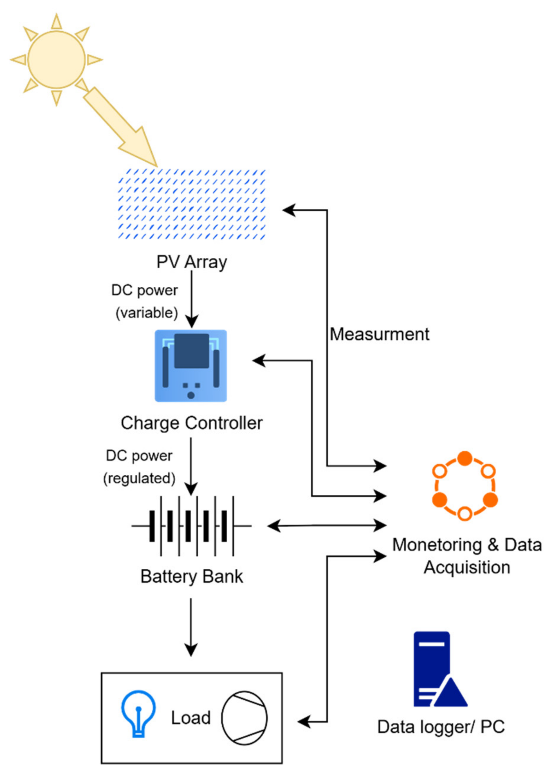
This study introduces the utilization of historical time-series data in the prediction of the power of a photovoltaic system by implementing an LSTM neural network approach. In contrast to traditional neural networks, LSTM method is effective in capturing and learning both short- and long-term sequential features through internal memory architecture. This makes the LSTM well adapted to forecasting cases containing nonlinear chronological data. The proposed methodology consists of three stages: data preparation, LSTM model formulation, and model evaluation. The overall system under study is shown in Figure 1.

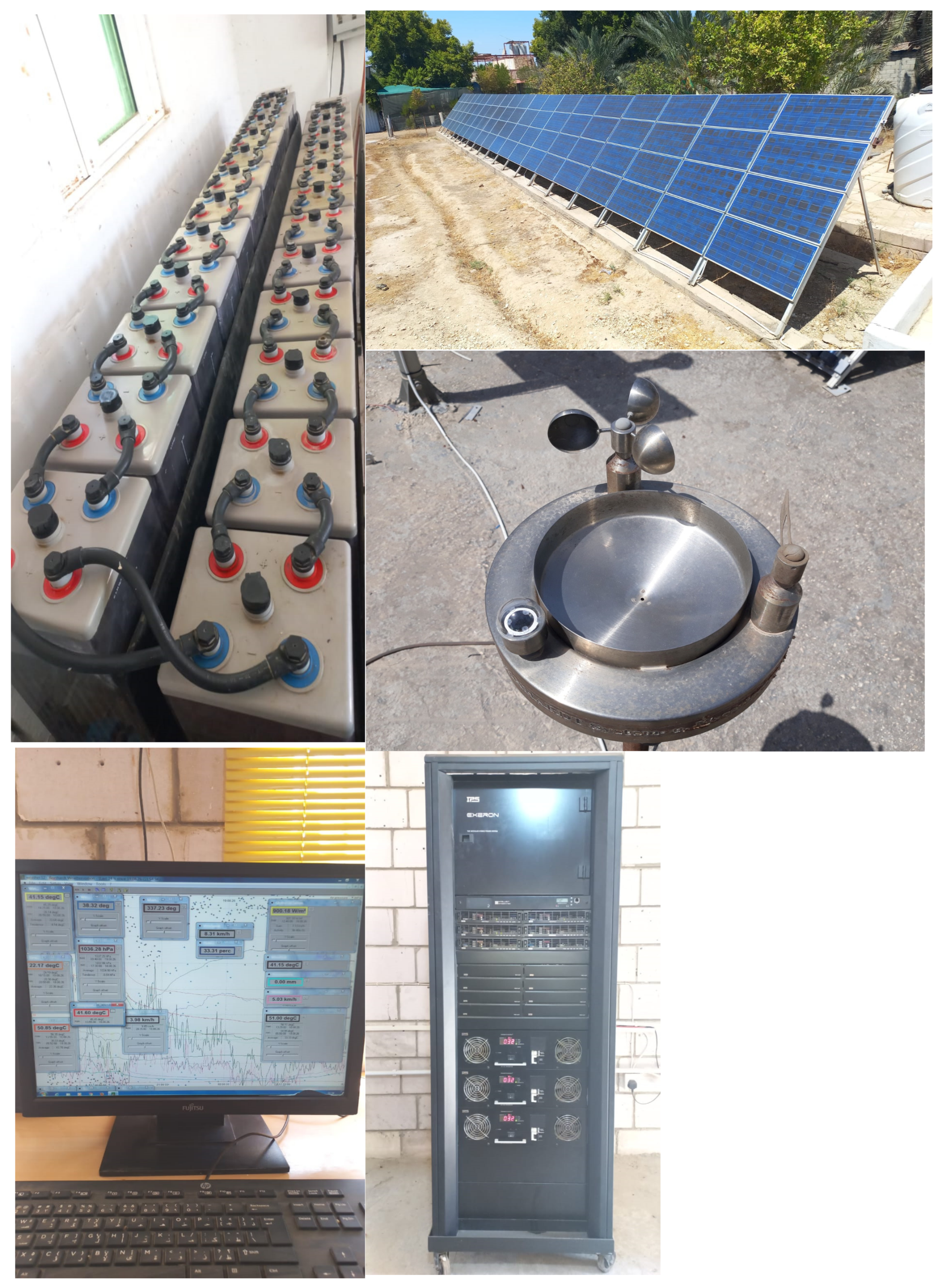
The system under study is shown in Figure 2. The PV system has capacity of 10 kWp powering the load demands, along with battery charging, which are used to power the load in the absence of solar power or in periods where solar power is not enough to drive the load. Battery charging is controlled through a charge controller, noting that the DC output is inverted to AC to meat the load input power. The system is also supported with a data acquisition system for data measurement, like power, solar irradiance, currents, and voltages.

2.2. Data Preparation

The proposed approach predicts power output by employing the historical operational variables gathered from the photovoltaic system. Dataset contains successive measurements recorded over consecutive time intervals, assisting the model to learn the time-based behaviour of the PV system. Based on the applied configuration, the LSTM input variables included historical PV power, solar irradiance, load demand, and temporal features, representing the hour of day and day of year, while the prediction target was the generated PV power.

Data are collected at the study site through a complete measurement system that collects the needed data for solar irradiance on 5 min basis, PV power output, PV voltage, charge controller voltage, battery currents, load consumption, and water supply data (

Table 1. Model input parameters.

Variable	Unit
Solar irradiance	W/m2
Batteries voltage	V
Batteries current	A
PV power production	W
Load power consumption	W
Time step	5 min

).

Initially, a continuous datetime variable was developed to set the accurate sequential order of the recorded observations to guarantee the temporal consistency. Dataset was then cleaned to remove the invalid or inconsistent records, which consequently enhanced the quality of the data and improved the stability of the learning mechanism. The cleaned time-series data were then down sampled to the desired forecasting resolution. Such procedure reduces the number of observations while preserving the temporal characteristics of the data.

Feature engineering is then developed to extract additional informative variables from the processed data, which improves the capability of the forecasting model to catch time-dependent behaviours of the PV system. Finally, the processed time-series data were converted into chronological input sequences, where each sequence consists of successive historical observations that serve as the input to the LSTM model.

2.3. Proposed LSTM Prediction Model

Because the LSTM can record both short- and long-term temporal connections within sequential data, it is the foundation of the forecasting model. In contrast to traditional neural networks, LSTM uses gating mechanisms and memory cells to retain significant previous data while eliminating irrelevant information.

The dataset was split chronologically into three parts: training (70%), validation (15%) and testing (15%). The oldest observations were included in the training part, then came the validation part, while the recent observations were assigned to the testing part. Such chronological splits helped to preserve the order of data and to avoid introduction of any information from the future observations.

The LSTM network utilizes forget, input, output, and memory cell operations to control the flow of information, as explained in the standard LSTM architecture [23,24]. The relevant equations are provided in Equations (1)–(6).

The network employs the current input vector, $x_t$, and the hidden state from the previous time step, $h_{t-1}$, at each time step. The quantity of information retained from the previous memory state is then determined by the forget gate ($f_t$) according to Equation (1).

$$f_t=\sigma \left(W_f\cdot \left[h_{t-1},x_t\right]+b_f\right)$$

(1)

The input gate ($i_t$) then controls the amount of newly obtained information retained in the memory cell, as expressed in Equation (2), whereas the candidate cell state (${\tilde{C}}_t$) is computed from the current input and previous hidden state using Equation (3).

$$i_t=\sigma \left(W_i\cdot \left[h_{t-1},x_t\right]+b_i\right)$$

(2)

$${\tilde{C}}_t=\mathit{tanh}\left(W_C\cdot \left[h_{t-1},x_t\right]+b_C\right)$$

(3)

The memory cell is then updated by combining the preserved historical information with the newly generated candidate information, as given in Equation (4).

$$C_t=f_t·C_{t-1}+i_t·{\tilde{C}}_t$$

(4)

The output gate ($o_t$) defines the information transmitted to the hidden state according to Equation (5), and the hidden state ($h_t$) is calculated using Equation (6), which denotes the output of the LSTM cell for the current time step.

$$o_t=\sigma \left(W_o\cdot \left[h_{t-1},x_t\right]+b_o\right)$$

(5)

$$h_t=o_t·\mathit{tanh}\left(C_t\right)$$

(6)

These sequences were provided as input to the LSTM network to learn the relationship between historical records and the corresponding PV power output, thus assisting the model to generate PV power predictions.

The developed architecture consisted of a single LSTM layer with 64 hidden units, along with the subsequent fully connected layer that had 16 neurons, along with ReLU activation layer. The sequence length of six data samples was considered, which was indicative of a historical period of 1 h with 10 min as sampling frequency. Adam optimizer was adopted for the training process of the model, and 0.001 was chosen as the learning rate with a mini-batch size of 512. The maximum number of epochs was 12; early stopping technique with patience value three was implemented, while no dropout layer was used.

2.4. Model Performance Evaluation

After the prediction stage, the predicted PV power values were compared with the corresponding measured values to evaluate the forecasting performance of the proposed model. The forecasting performance measures were computed, with the RMSE, MAE, and Mean Absolute Percentage Error ($MAPE$), as presented in Equations (7)–(9) [25]. The coefficient of determination ($R^2$) and Pearson’s correlation coefficient ($R$) were used to check the goodness of fit and the strength of the linear relationship between the predicted and actual values, respectively, as defined in Equations (10) and (11) [26].

The RMSE, provided in Equation (7), measures the square root of the average squared prediction error.

$$RMSE=\sqrt{{\displaystyle \frac{1}{N}}{\displaystyle \sum _{i=1}^N}{\left(y_i-{\hat{y}}_i\right)}^2}$$

(7)

The MAE is determined using Equation (8) and denotes the average absolute difference between the predicted and actual values.

$$MAE={\displaystyle \frac{1}{N}}{\displaystyle \sum _{i=1}^N}|y_i-{\hat{y}}_i|$$

(8)

The MAPE is calculated using Equation (9) and expresses the prediction error as a percentage of the actual value.

$$MAPE={\displaystyle \frac{1}{N}}{\displaystyle \sum _{i=1}^N}\left|{\displaystyle \frac{y_i-{\hat{y}}_i}{y_i}}\right|\times 100$$

(9)

The coefficient R² is presented in Equation (10), which measures how well the predicted values explain the variation in the actual PV power.

$$R^2=1-{\displaystyle \frac{{\displaystyle {\sum }_{i=1}^N}{\left(y_i-{\hat{y}}_i\right)}^2}{{\displaystyle {\sum }_{i=1}^N}{\left(y_i-\overline{y}\right)}^2}}$$

(10)

Finally, the Pearson correlation coefficient ($R$), presented in Equation (11), calculates the linear correlation between the predicted and actual PV power values.

$$R={\displaystyle \frac{{\displaystyle {\sum }_{i=1}^N}\left(y_i-\overline{y}\right)\left({\hat{y}}_i-\overline{\hat{y}}\right)}{\sqrt{{\displaystyle {\sum }_{i=1}^N}{\left(y_i-\overline{y}\right)}^2{\displaystyle {\sum }_{i=1}^N}{\left({\hat{y}}_i-\overline{\hat{y}}\right)}^2}}}$$

(11)

Lower RMSE, MAE, and MAPE performance measures represent lower errors, while higher values of R² and the Pearson correlation coefficient reflect a better fit of the model to the actual PV power values.

2.5. Battery and Energy Analysis

Battery and energy performance assessment is performed using measurements with the original resolution of 5 min. Battery state of charge (SOC) is determined from the measurement of battery current, assuming initial capacity of 200 Ah with initial state of charge of 60% and limiting the SOC within the operating range of 20% to 90%. The battery power was obtained from measured voltage and current, as defined in the equation:

$$P_{bat}=V_{bat} \left(t\right)·I_{bat} \left(t\right)$$

(12)

where $V_{bat} \left(t\right)$ and $I_{bat} \left(t\right)$ represent the measured battery voltage and current at time t, respectively. The corresponding current and power profiles were used to characterize the battery charging and discharging behavior during the study period.

Furthermore, the measured PV and load power were converted into energy using the 5 min sampling interval. The resulting energy values were accumulated monthly to calculate the variation in PV generation and load consumption over the full-year period.

3. Results and Discussion

3.1. Operational System Data

In this section, the raw solar irradiation, PV power generation, and the load profile are presented for the raw data measurement during the monitoring period.

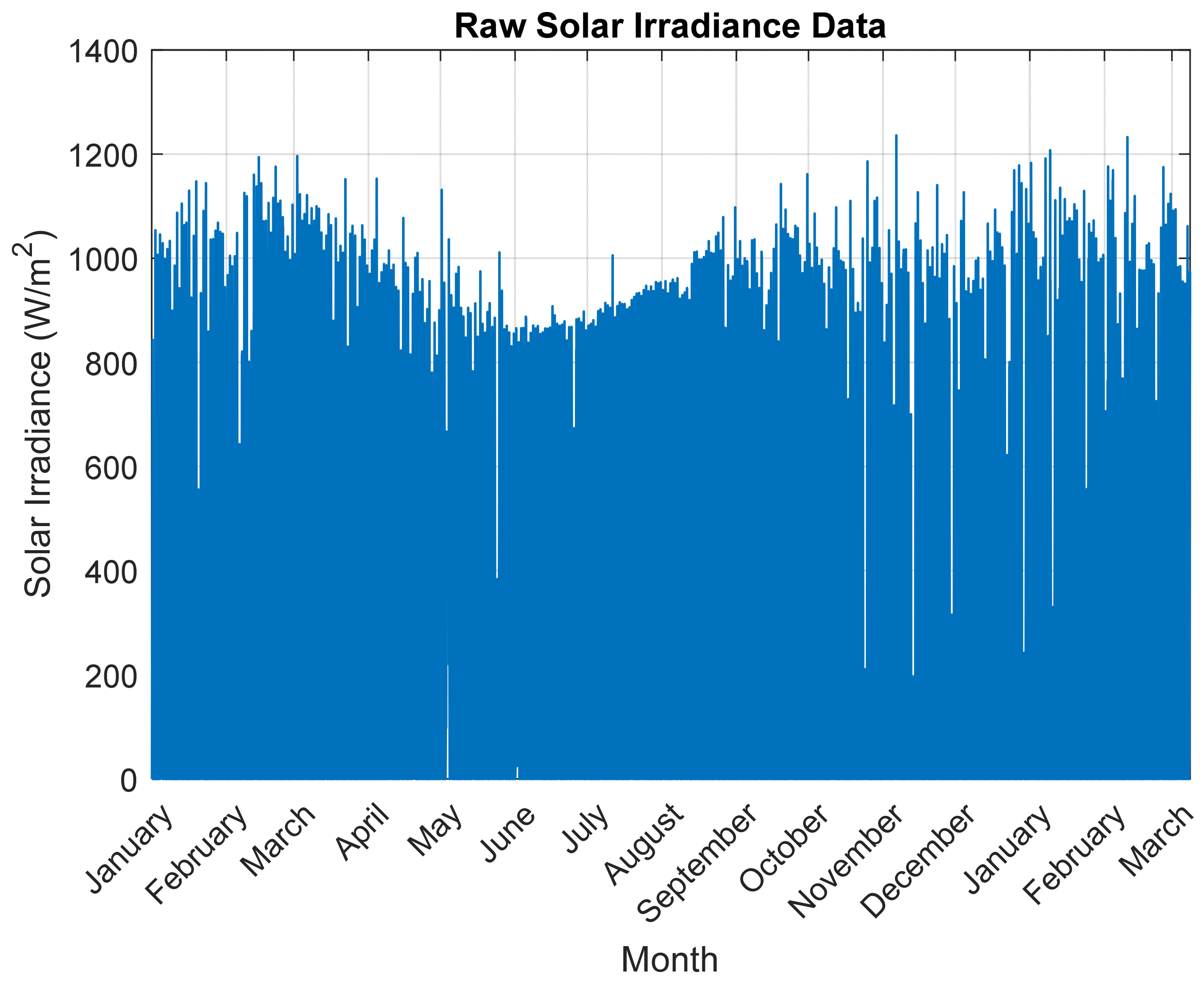
As shown in Figure 3, the measured solar irradiance over the entire monitoring period with a 5 min interval time resolution is presented. The measured values indicate a wide range of variability, ranging from zero levels during nighttime and low values during intermittent cloudy periods up to peaks exceeding 1200 w/m² under clear-sky conditions. The solar profile shows the profitable exploitation of PV systems, which verifies the use of PV technology for supplying the load demands. Having values above 800 W/m² for the whole year ensures stable power delivery that meets the load nature, mainly brackish water desalination. However, there is a noticeable period in winter, which is normal due to the cloud coverage times.

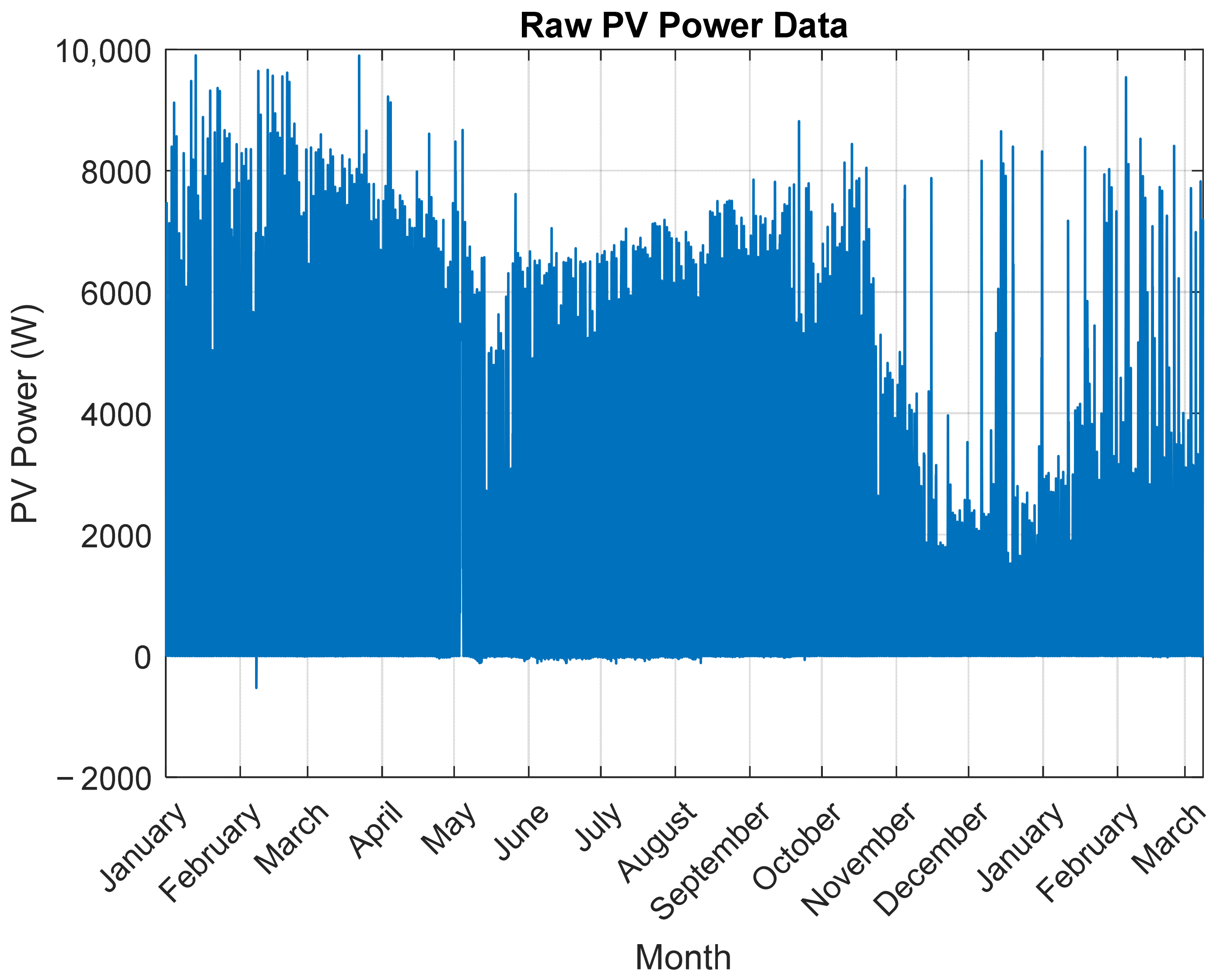
The PV-generated power shown in Figure 4 indicates significant daily and seasonal variability, which reflects the nature of solar energy and the influence of changing meteorological conditions. In high solar irradiance periods, peak power values approach 10 kW, whereas at night, it decreases, reaching zero. The seasonal trends show relatively high-power production during the first half of the monitoring period, ranging between 6 kW and 7 kW, followed by a noticeable reduction during the late autumn and winter months due to the shorter daylight hours and lower solar irradiance. The PV production has the lowest values in the period from November to February, reaching lower than 2 kW on average. This initiates the need to have continuous charging for batteries for covering the irrigation needs. It is worth mentioning that the irrigation profile decreases as well in the winter season, where plants benefit from rain. However, having a continuous fresh water supply can be achieved by relying on battery energy. There are short durations with fluctuations and occasional sharp power drops observed throughout the data, indicating the impact of transient cloud cover and other atmospheric disturbances. The high-frequency measurements effectively captured both long- and short-term variations, which provide a comprehensive dataset for training and validating the proposed LSTM-based forecasting model. The pronounced variability in PV generation emphasizes a further need for accurate forecasting to support efficient battery charging, energy management, and reliable operation for the system.

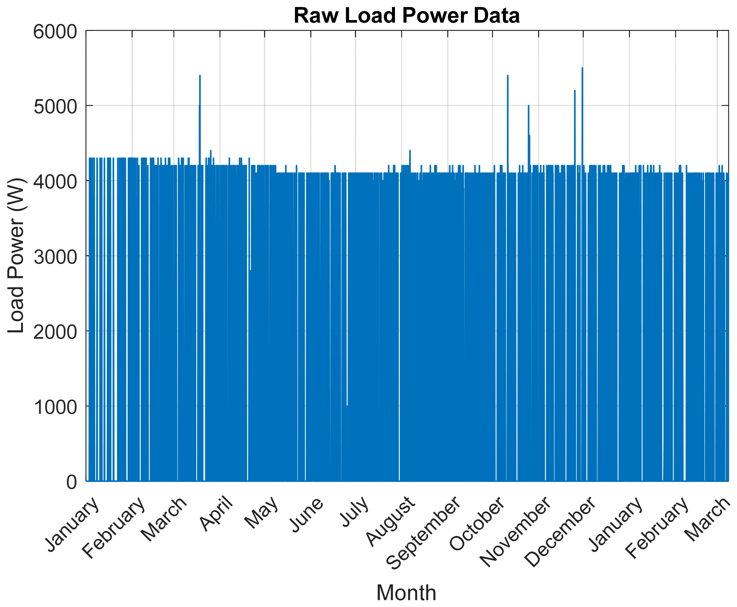
The load profile exhibits relatively stable operating behaviour, with an average demand of around 4.2 kW over the year, as illustrated in Figure 5. There are short-duration interruptions, and periods of reduced power consumption were observed, corresponding to intermittent load operation or temporary shutdowns of the electrical equipment. Furthermore, a limited number of transient peaks exceeding the nominal load level are identified, which indicates high-power application startup currents. In general, the load profile shows low seasonal variability, indicating that the electrical demand is primarily governed by operational requirements rather than environmental conditions, considering that the main load demand is powering water pumps used for water desalination. The relatively consistent load provides a suitable basis for evaluating the performance of the proposed LSTM-based PV power forecasting model and associated battery energy management strategy under realistic off-grid operating conditions. The associated load is basically the water pumps installed to operate the RO unit, including feeding pump and high-pressure pump, both with an approximately 4.2 kW power rating, as they rely on the induction motor construction. Samples with high peaks exceeding 4.2 kW are associated with the high starting current.

3.2. Forecasting Test Results

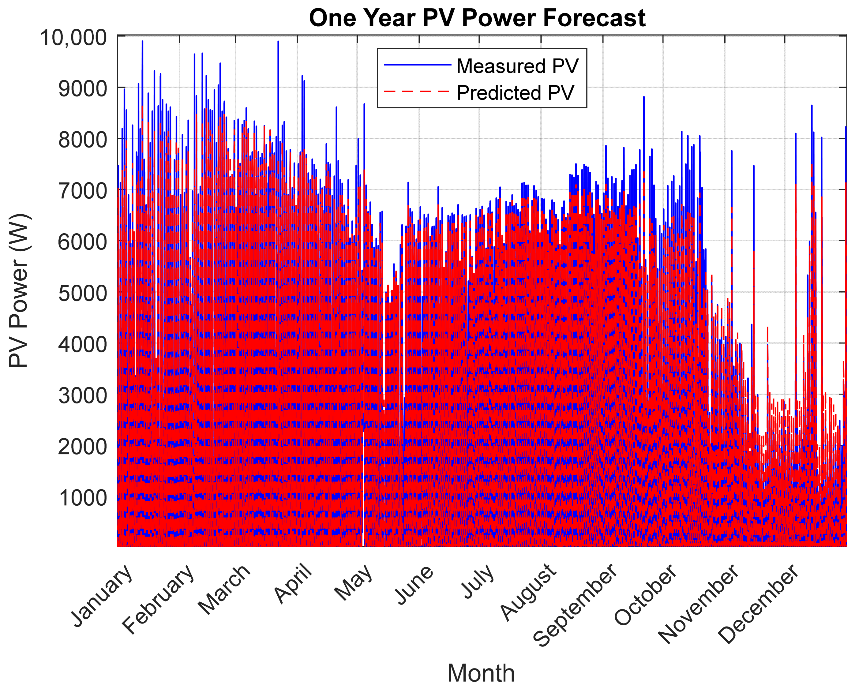
A comparison between the measured PV power and the predicted power is shown in Figure 6, where forecasting for the whole year is presented. It exhibits the characteristics of the daily generation pattern, with power increasing rapidly after sunrise, reaching peak values between 6 kW and 7 kW during most days. The measured PV power occasionally reaches between 9.5 kW and 10 kW and has power values between 2 kW and 3 kW in November and December. The predicted output generally follows the same temporal trend with slightly lower peak values, indicating a minor underestimation during periods of maximum generation. The forecasting model successfully reproduces the daily production cycles and captures the overall variation in PV output under different weather conditions. There are small deviations between the measured and predicted curves observed during sudden power fluctuations and high-power peaks, which are typically associated with the rapid changes in the solar irradiance caused by transient cloud cover. Nevertheless, the periodic profile remains in close agreement with the measured data throughout the testing period, demonstrating the capability of the LSTM model to accurately learn the nonlinear temporal characteristics of the PV power generation. This agreement is further supported by the obtained statistical performance metric R² = 0.728, indicating the sustainability of the proposed forecasting model for improving battery charging and energy management in standalone PV systems.

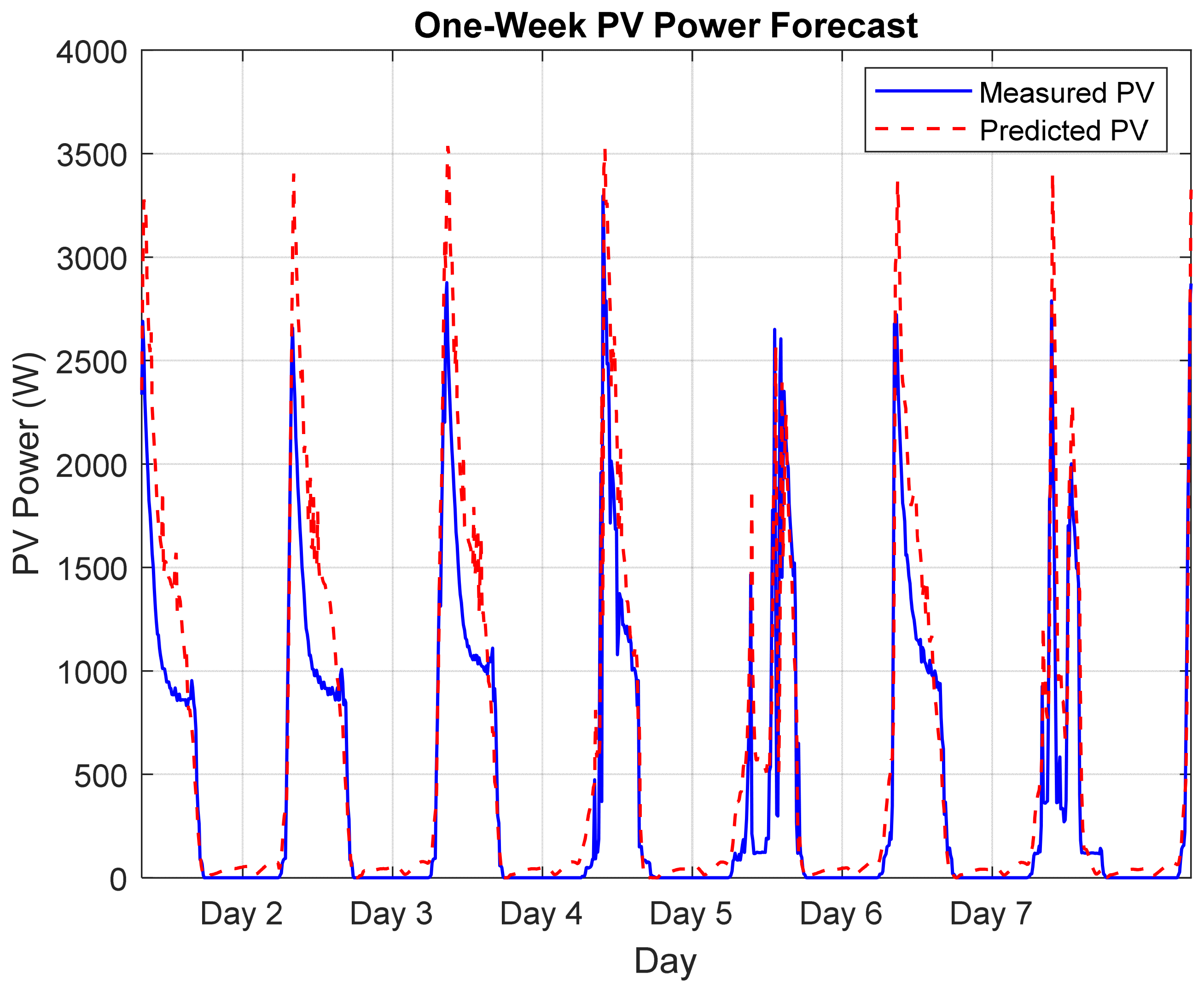
The predicted power profile follows the overall temporal behaviour of the measured PV generation, as shown in Figure 7, which is a representation of a one-week comparison between the measured PV power output and the values predicted by the proposed LSTM model as a sample taken from the annual overall forecasts. The daily production cycles are accurately reproduced and characterized by the near-zero output during nighttime and maximum generation during daylight hours. The measured PV power reaches peak values of approximately 2.6 to 3.4 kW, while the predicted output generally varies between 2.8 and 3.5 kW, indicating that the forecasting model captures the overall generation trend.

The model successfully identifies the onset and cessation of PV generation each day and accurately predicts the general shape of the daily power curve. There is a good correlation between the measured and predicted values during periods of relatively stable solar irradiance. The forecasting model accurately predicts the timing of peak generation with only minor deviations in peak magnitude, generally within 200–400 W for most days. Slight overestimation is observed on 6, 9, and 10 January, where the predicted peak power exceeds the measured values by approximately 5–10%, whereas a small underestimation occurs during periods of rapidly fluctuating PV output, particularly on 8 January, reflecting the influence of transient cloud cover and rapid irradiance variations. Despite these localized discrepancies, the forecasting model effectively reproduces the temporal dynamics of PV generation throughout the evaluation period.

Overall, the close correspondence between the measured and predicted power profiles demonstrates the capability of the proposed LSTM model to learn the nonlinear relationship between historical operating conditions and PV power generation. The forecasting accuracy is further quantified by the statistical performance obtained from the evaluation metrics R² = 0.728, approving the eligibility of the developed model for short-term PV forecasting and its potential application in predictive battery charging and energy management of the standalone PV system.

The smoothing effect that has been observed in the predicted PV power is attributed to the LSTM model learning dominant temporal patterns during high-frequency fluctuation filtering, considering atmospheric disturbances like cloud movements. Consequently, the model exhibits minor underestimation of short-duration power peaks, although the model accurately captures the overall daily generation profile.

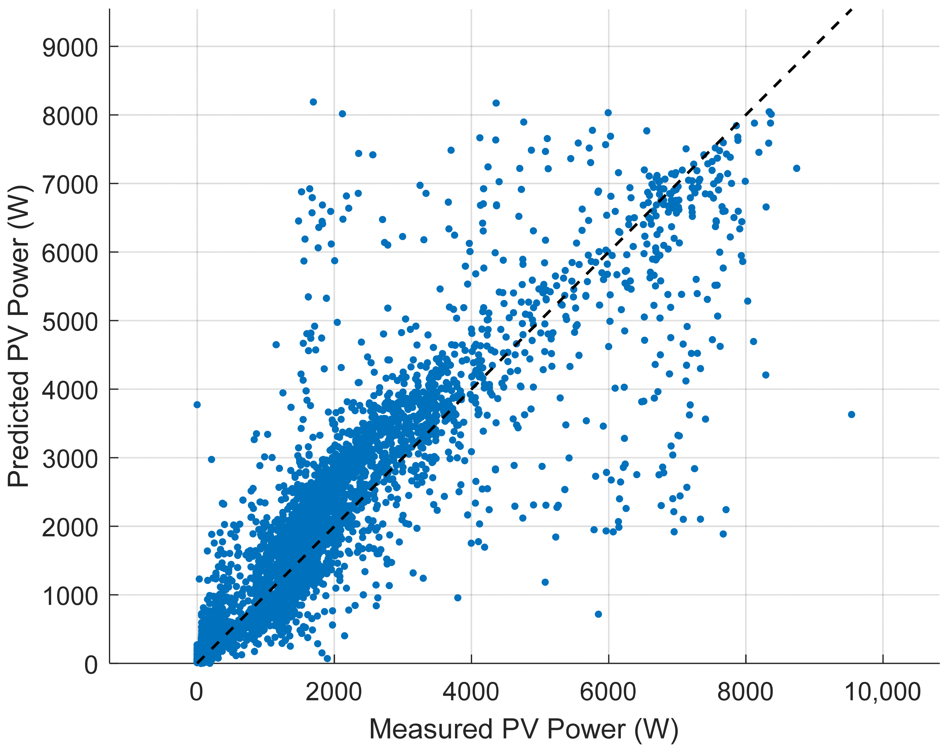
Figure 8 shows the correlation between the measured and the LSTM-predicted PV power during daylight, where each point represents a single forecast period with a 10 min interval, while the dashed diagonal line indicates the ideal one-to-one agreement between the measured and the predicted values. The measured PV power ranges from 0 to 8.5 kW, whereas the predicted values extend to approximately 8.2 kW, demonstrating that the proposed LSTM model succeeded in reproducing the overall operation range of the PV system. The obtained coefficient of determination (R² = 0.728) indicates that approximately 72.8% of the variability in the measured PV power is explained by the forecasting model, confirming a good correlation between the predicted and measured values. The highest concentration of data points is observed within the 0–4 kW range, where the predicted values are close to the one-to-one reference line, indicating high forecasting accuracy under low and moderate generation conditions. As the PV output increases beyond 5 kW, a larger dispersion of points is observed, reflecting the increased uncertainty associated with rapid irradiance fluctuations, transient cloud cover, and other atmospheric disturbances.

Nevertheless, most high-power observations remain distributed around the ideal correlation line, showing that the proposed LSTM model captured the nonlinear behaviour of the PV generation effectively over a wide operating range.

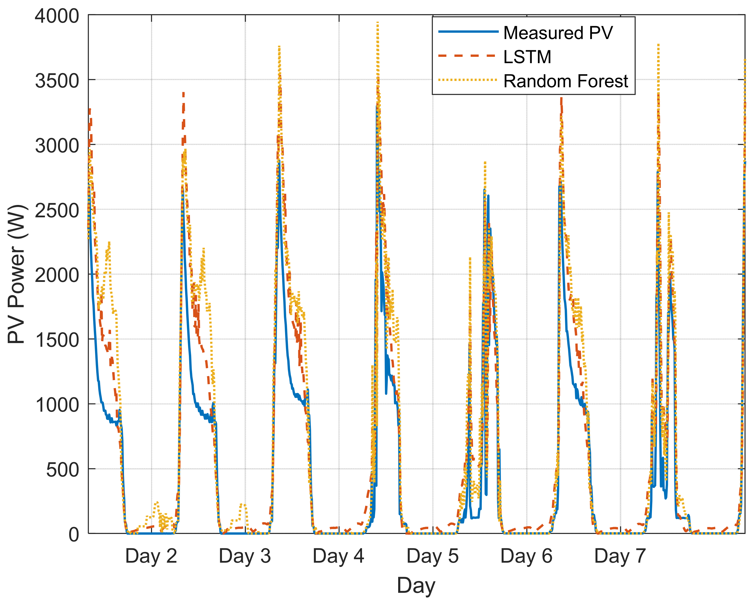
In Figure 9, the measured and forecasted PV output values by the LSTM and the Random Forest methods are compared for the chosen test period, considering the Random Forest method as a stable method for forecasting based on a time-series set [27,28]. At times of gradual change, both models show close similarity to the measured profile and accurately capture the pattern of PV production. On the other hand, at times when PV power changes abruptly, particularly during rapid increases, decreases and peak production periods, deviation is more apparent between the two. In such cases, it can be noticed that the LSTM model is closer to the measured profile, whereas the Random Forest model shows considerable deviation at various points. Generally, there are some deviations even in the case of the LSTM model at times of rapid changes, showing that it is difficult to forecast PV accurately in such instances.

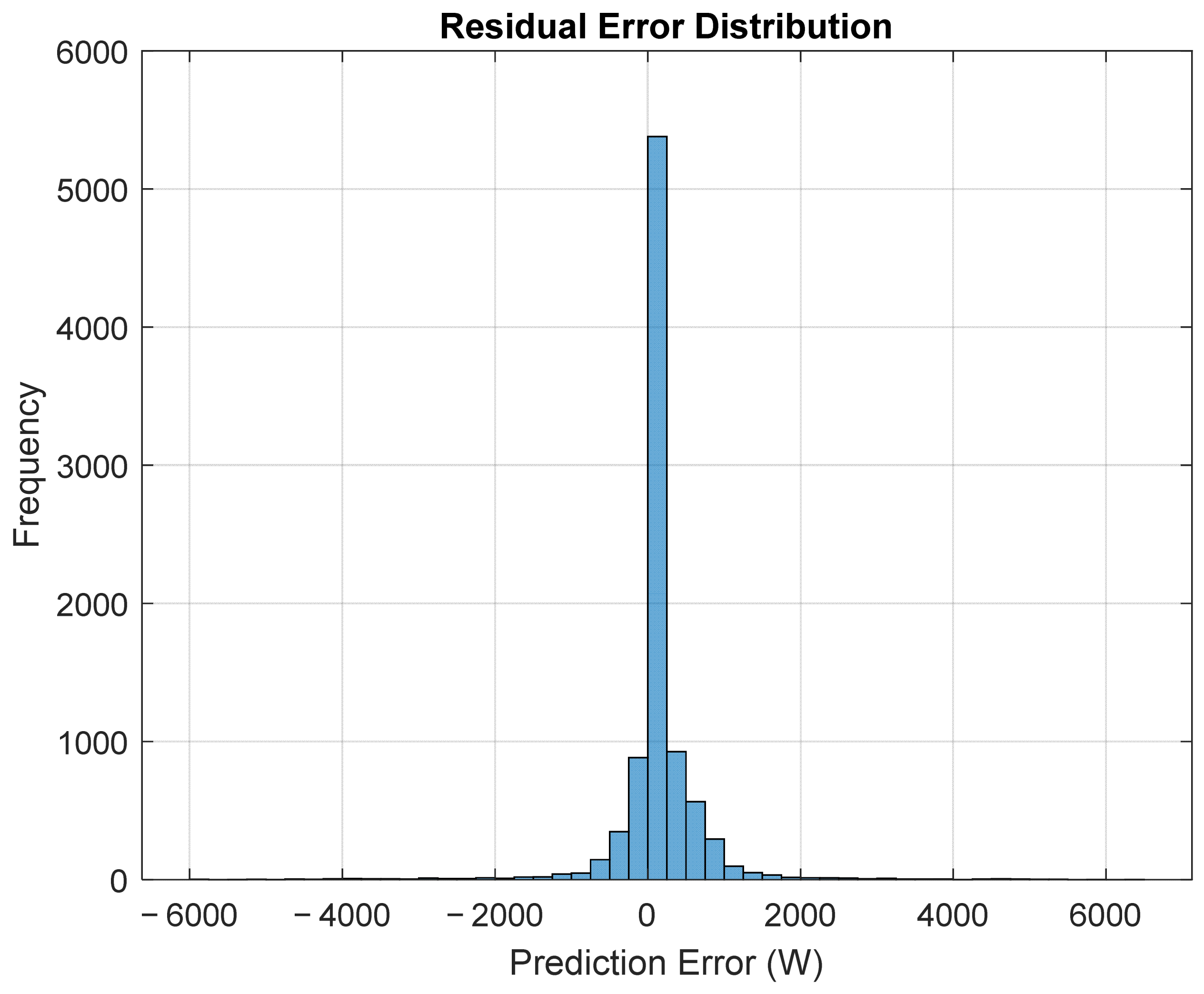
Residuals are calculated as the difference between the predicted and measured PV power values, as shown in Figure 10. The histogram exhibits a pronounced peak centred around 0 W, indicating that most forecasting errors are relatively small and that the model does not exhibit a significant systematic bias toward either overestimation or underestimation. Most errors are concentrated within approximately ±500 W, while the frequency decreases progressively as the prediction error increases in either direction. There is a limited number of larger residuals extending to approximately ±2 kW; only few isolated cases beyond this range are observed during periods of rapid irradiance fluctuations caused by transient cloud cover and changing atmospheric conditions. The distribution of the residuals is approximately symmetrical around zero, which demonstrates the forecasting errors are randomly distributed rather than exhibiting a persistent trend. The residual analysis indicates that the developed LSTM model provides reliable short-term PV power forecasting and is well suited for supporting battery charging scheduling and energy management in standalone systems.

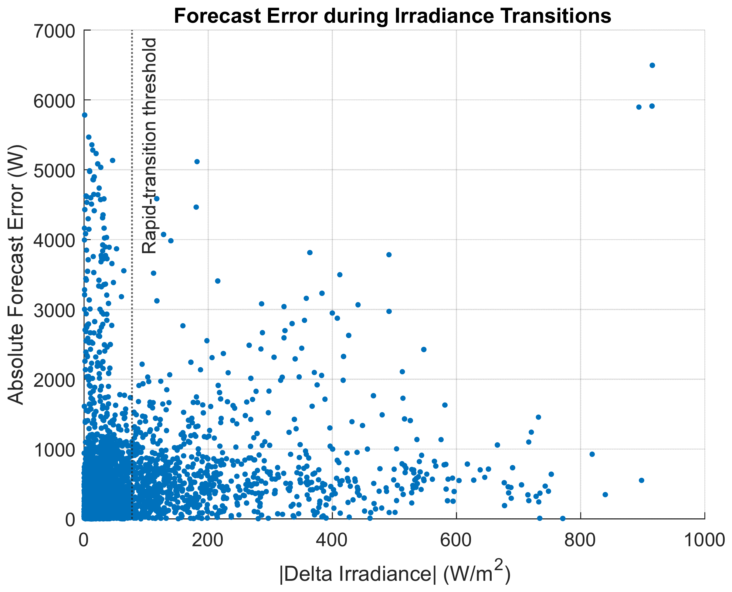
The absolute forecasting error with respect to variations in solar irradiance is shown in Figure 11. Most observations are concentrated at low error values and slight variations in irradiance. A greater range of values is seen around and beyond the rapid-transition threshold, and errors become more scattered as the irradiance variation rises. Higher irradiance changes also show several larger deviations. Overall, the distribution demonstrates that under comparatively stable irradiance conditions, lower forecasting errors are more densely concentrated, whereas larger irradiance variations are linked to a wider distribution of prediction errors.

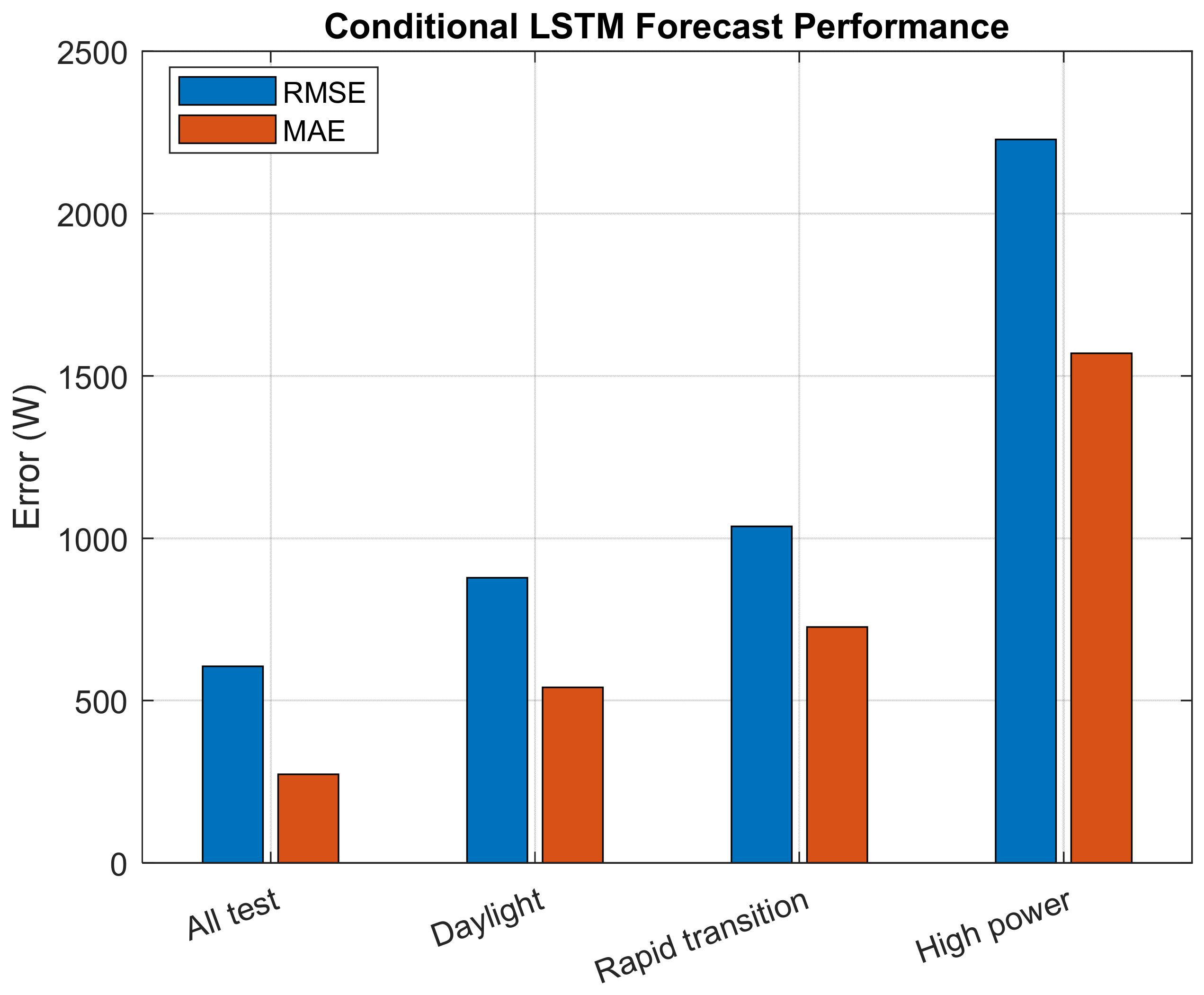
The achieved forecasting errors (RMSE and MAE) under several operating conditions are presented in Figure 12. Regarding the all-test dataset, the RMSE value is around 0.6 kW, while the MAE value is below 0.3 kW. Higher errors are observed during daylight hours. An additional increment takes place when irradiance changes at rapid transition; the RMSE value exceeds 1 kW, and the MAE value approaches 0.7 kW. The largest error values are registered in the case of high-power operation when the RMSE is larger than 2 kW, and the MAE is about 1.5 kW. The performance of the all-test dataset forecasted outputs was then compared to other LSTM PV studies. RMSE and MAE values of 0.7031 and 0.4473 kW were reported for a 5.83 kW system [29], whereas values of 1.255 and 0.889 kW were recorded for a 10 kW system [30]. Overall, the error values obtained in the current work are within a similar range and support the forecasting output achieved.

3.3. Battery Charging and Discharging Profile

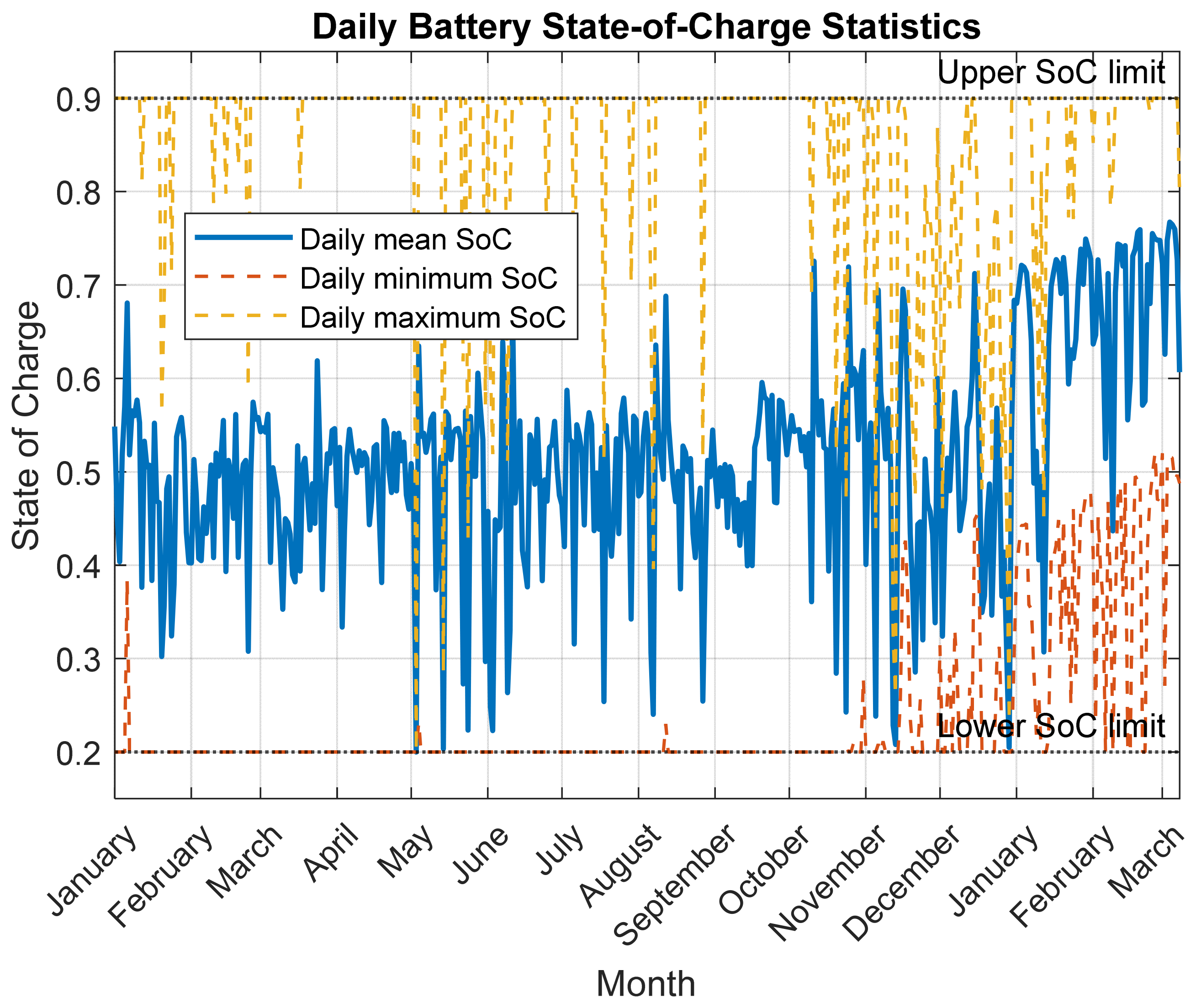
The state of charge (SOC) profile was determined through the measured battery current; the SOC was constrained within predefined operational limits of approximately 20% to 90%, thereby preventing excessive overcharging and deep discharge conditions (see Figure 13).

The obtained results show highly dynamic charging–discharging behaviour, which reflects the stochastic nature of PV generation and the continuous variation in the electrical load demands. During periods of high solar radiation, the battery is rapidly recharged, reaching the upper SOC limit frequently with 90%, indicating that the PV system is capable of simultaneously supplying the connected load and storing excess generated energy. Conversely, periods of reduced solar irradiance result in progressive battery discharge, causing the SOC to approach the lower operational threshold. The increased frequency of low-SOC events observed between November and February is consistent with the seasonal reduction in solar energy availability and shorter daylight duration.

Despite the significant temporal variability in both PV generation and load demand, the battery SOC remains predominantly within the prescribed operating limits throughout the monitoring period. This behaviour demonstrated the effectiveness of the adopted battery management strategy handled by the original control system in maintaining operational continuity while protecting the energy storage system from detrimental operating conditions. Furthermore, results highlight the critical role of battery storage in mitigating the inherent intermittency of PV generation, improving energy utilization, and ensuring a stable and reliable power supply for a standalone PV system. The SOC profile also confirms that accurate short-term PV power forecasting can provide valuable information for predictive battery charging and discharge scheduling, thereby enhancing overall system performance and extending battery service life.

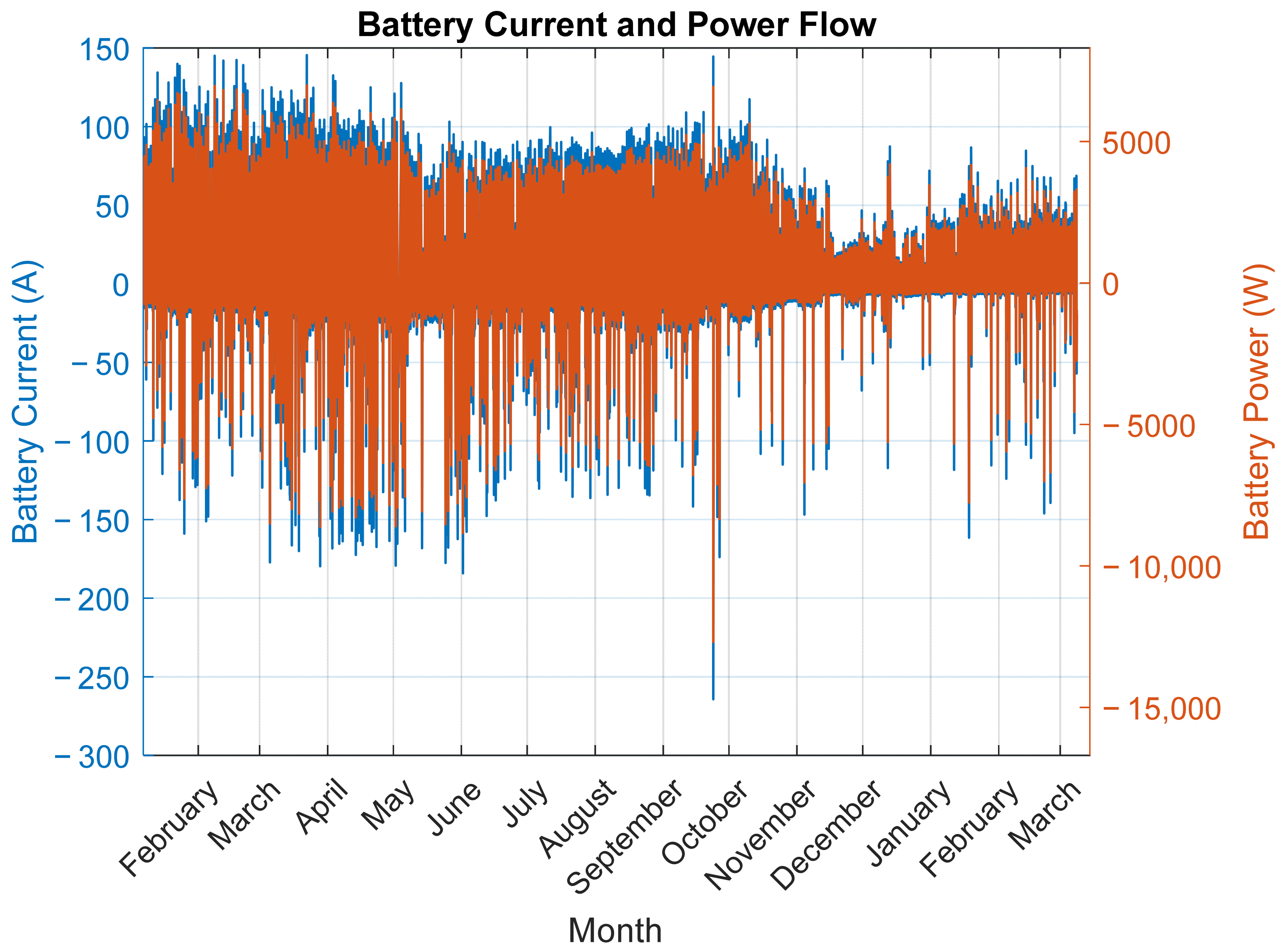
The temporal variation in the battery current and the corresponding battery power throughout the one-year monitoring period are shown in Figure 14. Positive values represent battery charging, while negative values indicate battery discharging. The achieved results show a highly dynamic battery operating profile characterized by frequent transitions between charging and discharging states. Battery charging current reached values of approximately +140 A, while peak discharging currents approached −270 A, corresponding to battery power levels exceeding +6 kW during charging and approximately −15 kW during discharge. The high peak transient events are primarily associated with periods of rapid changes in solar irradiance or sudden variations in load demand, considering the load nature of having induction motors that have high starting currents.

Having an overview of the seasonal variation, it appears that during periods of higher solar energy availability, particularly in spring and summer months, the battery operated predominantly under charging conditions, resulting from the excess PV energy after satisfying the electrical load demands. Conversely, increased discharge events were observed during the late autumn and winter months, when reduced solar irradiance limited PV generation and the battery became a source for maintaining continuous power supply, noting that the load demands are lower in winter months, which helps in having sufficient power from batteries. Despite these fluctuations, storage batteries exhibited stable bidirectional operation throughout the monitoring period.

Results further indicate that accurate short-term PV power forecasting can support predictive battery scheduling by anticipating charging opportunities during periods of high solar generation and optimizing battery discharge during intervals of reduced PV output, thereby improving system reliability, energy utilization and battery lifetime.

3.4. PV and Load Energy Summary

The annual PV energy production reached 13.3 MWh over the whole testing period, while the overall load energy was 4.43 MWh. The PV production serves both battery charging and load, and for periods under high solar irradiance, the load considered is only the water desalination plant as there are other facility loads not counted in this study as the main concern is the PV production power and delivery. Seasonal variation in energy generation was observed following the solar irradiance profile, with the highest monthly PV energy reached in July, while the lowest production occurred in winter, especially November and December. High energy production was observed during the spring and summer months due to increased solar irradiance and longer daylight hours.

The load demand exhibits moderate seasonal variation; the considered load demand is the water desalination plant, which has a constant profile power, as illustrated in Figure 4. The load demand is primarily driven by the operational requirements, with a brackish water desalination plant used for farm irrigation.

Results emphasize the importance of accurate PV power forecasting, which can be used for battery management. Actual battery behaviour is only presented in this study to balance the mismatch between variable renewable energy generation and relatively stable load demand, thereby ensuring continuous and reliable operation of the standalone PV system.

4. Conclusions

This study developed and evaluated a multivariate LSTM model for 10 min ahead PV power forecasting using one year of operational measurements collected from an off-grid PV system using batteries with a 5 min sampling time and for areas below sea level for the power water desalination plant. The proposed framework combined historical PV power, solar irradiance, electrical load, and temporal features to accurately model the nonlinear behaviour of PV generation under real operational conditions. The developed methodology incorporated comprehensive data preprocessing and sequence learning to support reliable short-term PV power forecasting.

The obtained results demonstrated that the proposed LSTM model effectively reproduced the temporal characteristics of PV power generation and achieved a daylight forecasting coefficient of determination of R² = 0.728, indicating good agreement between the measured and predicted PV power, considering that the plant under study has 10 kWp power capacity at ideal conditions; therefore, the maximum power generation might not be achieved due to climate factors, mainly solar irradiation and temperature values. In this study, power generation was mainly distributed between 6 kW and 7 kW, while it hit values above 9.5 kW in rare cases, and it reached below 2 kW in winter months, which naturally resulted from the solar profile. The forecasting LSTM followed the measured solar profile with significant consistence, and residual analysis further showed that the prediction errors were predominantly centred around zero, confirming the absence of significant systematic forecasting bias. The monthly energy analysis revealed the expected seasonal variation in PV energy production, while the electrical load exhibited smaller seasonal fluctuations due to the load demand requirements. In addition, the battery SOC remained within the prescribed operational limits of 20–90%.

The main contribution of this study is the integration of the forecast of short-term PV power generation and the performance of the standalone PV system. In this study, an LSTM neural network model was utilized for the prediction of PV power generation, and the real data from the system were studied to determine the performance of the battery during charge/discharge cycles as well as the correlation between the PV generation and the load demand. This approach makes it possible to obtain a more thorough understanding of the system performance by creating the basis for integrating PV forecasts into future performance evaluations.