


Abstract
Coastal lagoons are productive fisheries, yet lagoon complexes are often assessed as single units. We analysed 45 years (1980–2024) of areal yield and licensed-fisher counts in six Amvrakikos Gulf lagoons, Greece. All six declined at indistinguishable rates over the full record, but analyses restricted to 2010–2024 favoured divergent trends between two large and four small lagoons (7.9 AICc units better than the common-slope model; p = 0.0013), with estimated drifts of −0.061 and +0.091 yr−1, respectively. Mean areal yield in 2021–2024 relative to 2011–2020 fell 29–47% in large lagoons and rose 35–92% in small lagoons. Divergence was favoured in 48 of 56 overlapping windows and supported by year fixed effects (p = 0.0002), although exact lagoon-level inference gave p = 0.067. Licensed-fisher counts in both large lagoons remained constant during 2021–2024, raising the possibility of administrative carry-forward and leaving recent effort metrics unverified. Derived catch per unit effort showed no identifiable trend direction, preventing attribution of yield changes to effort withdrawal or resource decline. Environmental screening was inconclusive, and no equilibrium reference point was identifiable. The findings justify lagoon-specific monitoring but demonstrate neither an effect of size nor ecological recovery.
1. Introduction
Coastal lagoons are among the most productive aquatic ecosystems on Earth. Shallow, semi-enclosed and maintained by exchange across a restricted connection with the sea, they sustain primary production of 50 to more than 500 g C m−2 yr−1 and areal fishery yields commonly an order of magnitude above adjacent open coastal waters [1,2,3]. In the Mediterranean they have supported fisheries for millennia through fixed traps intercepting the seasonal migrations of mullets, eels, seabream and seabass, and remain central to the communities holding their concessions [4]. Their productivity has been attributed primarily to the gradients generated by confinement and exchange rather than to nutrient supply alone, which implies that lagoon yield should be sensitive to the geometry of the system and to anything altering its hydraulic connection with the sea [3].
That same confinement makes lagoons acutely vulnerable: shallow depth and limited flushing amplify nutrient loading, hydrological alteration modifies the freshwater and sediment input on which the salinity gradient depends, and warming acts directly on a water column with little thermal inertia. Set against these pressures is a fishing sector in its own long decline: Mediterranean lagoon fisheries have contracted widely [4], the Greek small-scale sector has lost vessels, fishers and catch [5], and reconstructed national catches indicate continuing recession rather than the recovery suggested by official statistics [6]. Disentangling a changing resource from a shrinking fishery is the central interpretive problem in any long-term analysis of lagoon landings.
The Amvrakikos Gulf in northwestern Greece offers an unusually well-defined setting in which to address it. It is a semi-enclosed, fjord-like embayment connected to the Ionian Sea by a single narrow channel, and its restricted exchange sustains a stratified water column with a persistent hypoxic to anoxic bottom layer that has demonstrably worsened: an area seasonally hypoxic in 1987 had become seasonally anoxic by 2009 [7,8]. Its northern and eastern margins carry lagoons differing by almost two orders of magnitude in area yet sharing one water body, climate and regulatory regime, and subject to datable interventions—the Pournari I and II dams on the Arachthos river (1981, 1998) and the Amvrakikos Wetlands National Park (2008). Long-term landings show a substantial decline attributed to fishing and other human pressures [9], and recent analyses document a reorganisation of catch composition and a decline in catch-derived production indicators around 2000 [10,11].
What that work has in common is the treatment of the complex as a single unit following a single trajectory, individual lagoons entering as replicates of it. This is a defensible summary of the twentieth-century record and is reproduced here. It may nevertheless no longer describe the present, and it carries a methodological consequence: a model with one fixed trend per lagoon cannot express “declined together, then separated”, and applied to the full series it will report a common trend whatever the most recent decade contains. Detecting a change in the relationship between subsystems therefore requires that the question be asked of progressively later windows.
The present analysis draws on the same complex and, for 1980–2020, the same records as two recent studies [10,11], five of the six present authors having contributed to both, so the boundary between what those studies established and what is added here is stated explicitly. Zoulias et al. [10] analysed 1980–2020 landings from Logarou, Rodia–Tsoukalio and the Mar Menor using trophic-level and Fisheries in Balance indicators and equilibrium Gordon–Schaefer models, concluding that the two Greek lagoons are low-yielding systems with declining yields and contracting fishing intensity. Zoulias et al. [11] extended the indicator approach to all six lagoons, adding primary production required, Kempton’s Q-90, the pelagic-to-demersal ratio, a chronological cluster analysis of species composition and a Ricker-type carrying-capacity estimate; it reported declining yield in every lagoon, a reorganisation of species composition around 2000, and exploitation states from over- to under-exploited. Both describe a complex settled at a reduced level of production, and [11] already concluded that one management strategy cannot serve all six lagoons.
Four elements of the present study are not contained in that work. The record is extended to 2024, and those four years make the separation substantially clearer, although some windows ending in 2020 already provide weak or marginal support. The six lagoons are contrasted as two size classes fixed a priori by area, a partition entering neither earlier analysis. Trend structure is estimated over progressively later windows, so that a change in the relationship between lagoons can be expressed and dated rather than averaged into a single slope. And the limits of what a landings series and a licensed-fisher count can support are established and reported rather than the statements they would otherwise license. The earlier catch-composition change is a decade or more older than the divergence window and is not advanced as its mechanism (Section 4.2).
Whether the components of such a complex respond coherently or divergently has direct ecological and management content. Where subsystems fluctuate asynchronously the aggregate is buffered by the portfolio effect that stabilises exploited stocks, and erosion of that asynchrony destabilises the whole [12]. A coherent decline implicates a gulf-scale driver: warming, basin-wide hypoxia, hydrological change or a common regulatory shift. A uniformly transmitted additive effect of such a driver cannot produce a class-dependent trend, since a gulf-wide variable takes the same value for every lagoon in a year; a common driver can nevertheless contribute where lagoons differ in sensitivity. It points either to local drivers or to differences among lagoons in how a common forcing is translated locally; both lead to the same lagoon-specific properties (inlet cross-section, depth, flushing time, distance from the river mouths, local effort dynamics), and both imply that management calibrated to the complex as a whole will be mismatched to some of its parts.
Two further problems shape the approach taken here. The first is the interpretation of landings: a decline is consistent both with a declining resource and with fishers leaving, and distinguishing them requires that landings, effort and catch per unit effort be examined jointly and the provenance of the effort record established. Examining the three jointly is not, however, the same as separating them: catch per unit effort is computed from landings and effort and is not an independent observation, and a count of licensed fishers is a proxy whose insensitivity to fishing days, gear and intensity enters any comparison directly. The second is the estimation of reference points: equilibrium surplus-production models overestimate surplus production and FMSY when fitted to declining stocks and are poorly identified when effort contrast is low, precisely the conditions in concession fisheries with administratively fixed crews [13]. Both are compounded by the short duration of most lagoon series, which invites the shifting-baseline error [14].
This study analyses 45 consecutive years (1980–2024) of yield and effort data from six Amvrakikos lagoons, Logarou, Rodia–Tsoukalio, Vathi, Pogonitsa, Mazoma and Tsopeli, extending by four years the record available to previous analyses. The objectives are: (i) to characterise long-term trends in areal yield, effort density and catch per unit effort, using methods appropriate to strongly autocorrelated series; (ii) to test whether the lagoons have continued to follow a common trend or have separated according to size, and if so when; (iii) to establish how far the available records constrain any apportionment of change between the resource and the withdrawal of effort; (iv) to test whether gulf-wide climatic and hydrological covariates can account for any divergence, and whether equilibrium reference points are identifiable at all; and (v) to state how these results relate to the two previous analyses [10,11]. We hypothesise that coherence characterises the earlier record, whereas later windows may separate the predefined size classes. Trend structure is tested over three progressively later windows whose boundaries use calendar-decade markers, although the decision to examine later windows followed whole-record models describing a single coherent decline and is therefore a response to the data (Section 2.6.2). Area is used only as the a priori criterion defining the groups and as a label for the correlated properties accompanying it (Section 2.1 and Section 4.5).
2. Materials and Methods
2.1. Study Area
The Amvrakikos Gulf (39°00′ N, 20°58′ E, northwestern Greece) is a semi-enclosed, fjord-like embayment of about 405 km2 connected to the Ionian Sea by the narrow Preveza channel. Restricted exchange, combined with freshwater input from the Arachthos and Louros rivers, maintains a stratified water column and a persistent hypoxic to anoxic bottom layer [7]. Its northern and eastern margins support shallow lagoons exploited for millennia by fixed-trap (ivari) fisheries targeting mullets (Mugilidae), European eel (Anguilla anguilla), gilthead seabream (Sparus aurata) and European seabass (Dicentrarchus labrax) (Figure 1).
Figure 1.
Study area: bathymetry and topography of the Amvrakikos Gulf (western Greece), showing its coastal lagoons, the main river mouths and the Preveza Strait connecting the gulf to the Ionian Sea.
The complex is a Ramsar site and, since 2008, the Amvrakikos Wetlands National Park. Six lagoons with continuous exploitation records were analysed (Table 1). Areas were taken from Zoulias et al. [11] and span 0.40 km2 (Pogonitsa) to 29.28 km2 (Rodia–Tsoukalio), with a 14.06-fold gap and no intermediate system, so lagoons were assigned a priori to two size classes, large (>20 km2; n = 2) and small (<2 km2; n = 4), on this externally measured trait rather than any property of the yield series. The classification records a bimodality in a measured trait, not a hypothesis that area is causal; areas differ within the classes too, so the design is a two-level contrast with n = 2 and n = 4 and area is a label for correlated morphological and hydrological properties (Section 4.5).
Table 1.
Morphometric and sampling characteristics of the six Amvrakikos Gulf lagoons analysed (1980–2024). Areas follow Zoulias et al. [11]. Effort density is the mean number of licensed fishers per square kilometre over the full record.
Given the limited replication within the large-lagoon class (n = 2), between-class comparisons may be disproportionately influenced by individual lagoon trajectories; this potential leverage was explicitly evaluated through leave-one-lagoon-out sensitivity analyses (Section 2.6.7).
2.2. Fishery Data
Annual statistics were compiled for the 45 years 1980–2024 (n = 270 lagoon-years), comprising per lagoon and year areal yield in tonnes per square kilometre (t km−2) and the number of licensed fishers, the index of nominal effort. The number of licensed fishers represents institutional nominal effort rather than directly observed fishing activity, because annual information on active fishing days, gear units deployed and fishing intensity was unavailable. Consequently, using this administrative indicator as a proxy for effective fishing effort or fishing mortality introduces unquantified measurement error, preventing direct estimation of actual fishing pressure from the licensing records alone. The 1980–2020 records are those compiled for the two previous studies of this complex [10,11]; the 2021–2024 update came from the same sources. Landings and licensing records were supplied by the Fisheries Departments of the Regional Units of Arta and Preveza, which hold the annual returns of the concessions. The landings were cross-checked against the production records of the concession-holding co-operatives; the licensing records were not, so the recent fisher counts remain unverified against concession documents (Section 3.4.2 and Section 4.3). Because these concession fisheries are worked exclusively through fixed traps at the lagoon outlets, the landings series is close to a census of the commercial catch; its weaknesses lie in the effort record (Section 2.6.6).
Four of the 540 entries were missing—yield and effort for Rodia–Tsoukalio in 2018, yield for Vathi in 2000 and for Mazoma in 1993 (Table 1).
Missing values were filled by linear interpolation between adjacent years with na_interpolation in the imputeTS package, version 3.4 [15], called with option = “linear” and maxgap at its default of Inf, independently within each lagoon series after ordering by year. All four missing values—yield and effort in Rodia–Tsoukalio 2018, yield in Vathi 2000 and yield in Mazoma 1993—formed interior gaps of a single year, no series beginning or ending with a missing value, so no gap-length limit was engaged and no extrapolation beyond the observed range was performed; each imputed value is accordingly the arithmetic mean of its two bracketing observations (Table S38). Every imputed value was flagged, listed in Table 1 and marked with open symbols in all figures, so no inference rests on an unidentified interpolated point. Imputed values were used in all analyses except the state-space models of Section 2.6.4, where missing observations were handled by the Kalman filter and raw series supplied. Because an interpolated point can in principle carry a trend result, all trend tests and all divergence models were refitted on the non-interpolated series (Section 2.6.11).
2.3. Derived Variables
Because yield was expressed per unit area while effort was an absolute count, the two were not comparable across lagoons differing 70-fold in size. Effort was converted to effort density (fishers km−2) by dividing licensed fishers by lagoon area, and catch per unit effort (CPUE) computed as areal yield divided by effort density. An absolute CPUE (t fisher−1) was retained for the decomposition of Section 2.6.6, in which absolute landings were reconstructed as areal yield times area.
2.4. Environmental Covariates
Eight annual candidate covariates were compiled for 1980–2024 to test whether large-scale climatic, hydrological or regulatory forcing could account for the yield dynamics.
Two describe atmospheric circulation: the North Atlantic Oscillation index [16] from the monthly NOAA Climate Prediction Center series, as an annual mean and a winter index (NAO_DJFM; December of the preceding year plus January–March).
Two describe thermal conditions: mean annual and maximum summer sea-surface temperature (SST; °C) from Level-3 monthly MODIS-Aqua composites (about 4.6 km; thermal infrared 11–12 μm daytime product) distributed by NASA, subset to the gulf (38.8500–39.0667° N, 20.7500–21.1833° E). Only valid marine pixels were retained; monthly Gulf SST was their mean, and the two covariates the mean of the twelve monthly values and the highest June–August value. Because the record begins in July 2002, both were considered available from 2003, so annual means rest on complete calendar years and summer maxima on complete June–August periods; the one pre-2003 value the compiled file carried was excluded before any analysis and is recorded in Table S1. No attempt was made to extend the series backwards with another sensor or reanalysis product.
One covariate describes rainfall: total annual precipitation (mm yr−1) from the ERA5 reanalysis [17], extracted at a fixed location representing Arta (39.16° N, 20.99° E) and aggregated to calendar-year totals.
Annual river outflows of the Arachthos and Louros were considered but are not included. The only accessible source for 1980–2007 is the plotted series of Katselis et al. [9], whose underlying monthly data were supplied to those authors by the Public Power Corporation S.A., Athens, Greece; values read from a published figure cannot be assigned a defensible measurement error, and no numerical record was obtainable for any part of the study period. Both series were therefore excluded from the covariate set, and freshwater delivery is represented here by precipitation alone, which was not spatially averaged over the gulf but represents a fixed terrestrial location.
The remaining three are binary intervention variables: Pournari I (0 for 1980, 1 from 1981), Pournari II (0 to 1997, 1 from 1998) and the National Park designation (0 to 2007, 1 from 2008, per Joint Ministerial Decree 11989/2008, Government Gazette 123/D/21-03-2008).
Salinity and bottom-water dissolved oxygen were excluded: though mechanistically plausible, observations were spatially restricted and temporally discontinuous, and were not interpolated to construct artificial continuous series. Coverage was audited before fitting, a covariate being usable in the divergence analysis only with at least eight observations and more than one distinct value inside that window. The SST series therefore began in 2003, and the intervention variables provided no usable variation within the divergence window and were excluded from it while remaining available for full-record analyses.
2.5. Trend Analysis
Monotonic trends in yield, effort density and CPUE were tested per lagoon with the Mann–Kendall test [18,19]. Because annual fishery series are strongly serially correlated, which inflates the Type I error rate of the classical test, the variance-corrected modification of Hamed and Rao [20] was the inferential test (modifiedmk [21]); the classical statistic is reported alongside, with the Durbin–Watson statistic [22] of a linear fit recording the serial dependence present.
Trend magnitude was estimated by the Theil–Sen slope [23,24], with confidence intervals from a residual moving-block bootstrap with 2000 replicates [25,26]: the trend was removed, contiguous blocks of residuals of length L = round(n(1/3)) (L = 4 for n = 45) resampled, the trend added back and the slope re-estimated. Resampling was non-circular: block start positions were drawn with replacement from the first n − L + 1 = 42 indices, so that every block lay wholly within the observed series and no wrap-around between the last and the first year was introduced. Twelve blocks (n/L rounded up) were concatenated and the resulting sequence truncated to the original length, so each replicate contained exactly n = 45 residuals. Because the scheme is non-circular, residuals at the two ends of the series enter fewer blocks than interior ones, the first and last residual each appear in one of the 42 blocks against four for residuals at positions 4 to 42, and since the trend is removed before resampling and added back afterwards, this affects only the variance contributed by the edge residuals. A rank test and a bootstrap interval are not two expressions of one inference, so the Hamed–Rao p-value is the single declared decision rule throughout and a Theil–Sen interval states magnitude rather than testing again. Two further intervals were computed by the rank-based construction of Sen [24], with the classical and with the Hamed–Rao corrected variance of the Mann–Kendall S statistic, and the bootstrap interval’s sensitivity to block length examined over L = 2–12 years (Tables S2 and S3). Tests were run over the full record and over the post-2000 period.
2.6. Divergence Analysis
The central hypothesis is that the six lagoons ceased to behave as a single unit in the most recent part of the record, the two large systems continuing to decline while the four small ones showed positive recent yield trends. Nine complementary analyses were used to test it.
2.6.1. Period Means and Recovery Ratios
The record was partitioned into five periods (1980–1990, 1991–2000, 2001–2010, 2011–2020, 2021–2024) and mean yield computed per lagoon and period. A recovery ratio was defined as the 2021–2024 mean divided by the 2011–2020 mean, with a 95% percentile bootstrap interval from 2000 resamples; values above unity indicate higher mean yield than in the preceding decade.
The terminal period is four years long and the baseline ten, so five further analyses establish whether the comparison depends on that binning. Mean yield was computed in every overlapping four-year window of the record and the terminal window ranked among them. The 2021–2024 mean was then divided by each of the seven four-year baselines contained in 2011–2020, which equalises the two periods at seven successive positions of the baseline, and by baselines lengthened from four to ten years ending in 2020. The ratio was re-estimated with a circular moving-block bootstrap at block lengths of two, three and four years, each period resampled within itself so that the interval carries the serial dependence that independent resampling removes; the same scheme applied to the two periods pooled, which imposes no level change, gives the distribution of ratios that short-term fluctuation alone produces in each series. Finally, the ratio of the 2021–2024 mean to the 2017–2020 mean was placed in the distribution of every adjacent four-year block ratio of the record, mean(t…t + 3) divided by mean(t − 4…t − 1); those windows overlap, so that distribution is a descriptive reference and not a test. These analyses are reported in Tables S40–S43 and Figures S15–S17.
2.6.2. Slope Structure Across Nested Windows
A divergence is a change in behaviour, not a constant differential trend, and a model with one fixed slope per lagoon fitted to the whole record cannot express “declined together, then separated”. Slope structure was therefore tested over three progressively later windows (1980–2024, 2000–2024, 2010–2024). Within each, log yield was modelled by generalised least squares, fitted by maximum likelihood, with a first-order autoregressive within-lagoon error structure (nlme [27]) under three specifications: a common time slope with lagoon-specific intercepts, a slope per size class, and a slope per lagoon. Models were compared by AICc [28,29] and, for the nested pair, by a likelihood-ratio test of the time × size-class interaction. The windows follow the decadal boundaries of Section 2.6.1 rather than any inspection of fitted slopes, but the windowed analysis was introduced after whole-record models had described a single decline, so it was a response to the data; sensitivity to the boundaries and to individual lagoons is assessed in Section 2.6.7.
2.6.3. Exact Enumeration of Alternative Groupings
Six lagoons split into a pair and a quartet in C = 15 ways. All 15 partitions were enumerated and the model pair refitted over 2010–2024 for each, recording the difference in mean log-yield slope and the interaction p-value, to establish whether the observed partition is exceptional. Because the size classification is fixed a priori by an externally measured trait, the interaction test remains the inferential test and the enumeration is supporting evidence; the smallest attainable exact one-sided p-value for a pre-specified 2-versus-4 split is 1/15 = 0.067.
2.6.4. Multivariate Autoregressive State-Space Models
Multivariate autoregressive state-space (MARSS) models were fitted to the log-yield matrix with the MARSS package [30], using identity state-transition and observation matrices and diagonal-and-equal process and observation variances. Three drift structures—common, by size class, and per lagoon—were compared by AICc over each window, the full-record comparison being a contrast rather than the test. Raw series were supplied, missing values handled by the Kalman filter, and approximate drift standard errors obtained from the package’s Hessian-based routine. Because the diagonal-and-equal specification constrains every lagoon to the same process and observation variance, which a seventy-fold range in area makes a strong assumption, it was examined rather than asserted. The per-lagoon residual variance of log yield about a lagoon-specific linear trend was computed in each window, with a Fligner–Killeen test of homogeneity and its rank correlation with area, and the three drift structures were refitted over a grid of variance specifications: Q as diagonal and equal, diagonal and unequal, equal variance and covariance, or unconstrained, crossed with R as diagonal and equal or diagonal and unequal, seventy-two fits in all. Convergence status and the smallest estimated variance were recorded for each, since an unconstrained Q estimates twenty-one variance parameters from six series and need not be identifiable (Table S16b).
2.6.5. Morphometric Contrast
The relationship between size and recovery was examined by regressing the recovery ratio on log10(area), by leave-one-out refitting, by refitting within the four small lagoons alone, and by a Wilcoxon rank-sum test of the two classes [31] as a two-sided exact test on ratios containing no ties; with groups of two and four the normal approximation is inappropriate and is reported only for comparison, the exact value being verified by complete enumeration of all fifteen assignments (Table S4). This battery was applied because a six-point regression across two well-separated clusters can produce an apparently strong relationship carried entirely by the gap between them.
2.6.6. Landings, Effort and CPUE Decomposition
A decline in landings admits two explanations: a declining resource, or the withdrawal of fishers. For 2010–2024, absolute landings, licensed fishers and absolute CPUE were each regressed on year per lagoon, and percentage change computed between the means of the first and last three years. Patterns were summarised descriptively as landings falling with CPUE rising, both falling, both rising, or mixed; these describe the joint behaviour of three recorded series and are not an attribution of cause (Section 2.6.10). Because a CPUE trend is interpretable only when effort is measured, an effort-provenance audit compared, per lagoon, the proportion of years in which the count changed before the final four years with its constancy over those last four. No lagoon was assumed to have verified-constant effort. The audit is reported as a probability rather than as a pass/fail classification, and no threshold was applied: in all six lagoons the terminal run of identical counts is improbable under that lagoon’s own pre-run rate of change (Section 2.6.10, Table S19), so no cut-off would separate one subset of the series from another and the recent effort record is treated as unverified throughout.
2.6.7. Sensitivity to the Analytical Period and to Individual Lagoons
Three sensitivity analyses established whether the divergence depends on the analytical window or on individual lagoons. First, the model pair was refitted over every combination of a first year from 2005 to 2015 and a last year from 2019 to 2024, discarding windows shorter than nine years and yielding 56 windows; the first margin tests dependence on the start year, the second removes terminal years. For each window the AICc difference, the interaction p-value and the difference in mean ordinary least squares slope between classes were recorded.
Second, the model pair was refitted over 2010–2024 six times, each with one lagoon removed. Because only two lagoons are large, removing either leaves a one-versus-four contrast, a different design rather than a weaker version of the same one, so the lagoons remaining in each class and the sign of the slope difference are reported alongside each p-value. Third, the MARSS comparison was refitted over 2010–2023. The recovery ratios were not subjected to the terminal-year analysis, since removing 2021–2024 deletes the statistic rather than testing it.
2.6.8. Dependence Among Repeated Observations and Among Lagoons
Two forms of dependence are present. Serial dependence within lagoons is addressed by every model in Section 2.5, Section 2.6.1, Section 2.6.2, Section 2.6.3, Section 2.6.4, Section 2.6.5, Section 2.6.6 and Section 2.6.7, through the autoregressive error structure and the Hamed–Rao correction; contemporaneous dependence among lagoons exposed in the same year to the same gulf-wide conditions is not, since the autoregressive structure is within lagoons and the state-space models assume diagonal covariances. Both were quantified before being modelled—the first by the autoregressive parameter and each lagoon’s lag-one residual autocorrelation, the second by the fifteen pairwise correlations among residuals in the same year, tested against a null generated by permuting each lagoon’s series independently. Effective sample sizes were n(1 − φ)/(1 + φ) and m/[1 + (m − 1)].
The difference in log-yield slope between the four small and the two large lagoons over 2010–2024 was then estimated under nine specifications: the autoregressive within-lagoon structure used throughout; the same with year fixed effects, absorbing any influence common to all six lagoons in a given year; a random year intercept crossed with lagoon; compound symmetry among lagoons within a year; unstructured cross-lagoon correlation; cluster-robust standard errors by year and by lagoon; a residual bootstrap over contiguous two-year blocks, retaining all lagoons within each sampled year and preserving both forms of dependence without modelling either; and a test treating each lagoon as a single unit, two slopes compared with four by exact enumeration, whose floor is 1/15 = 0.067 and which is the form appropriate to six spatial units. Lagoon-clustered standard errors used a t reference with five degrees of freedom and are indicative only with six clusters. The state-space comparison was also refitted with an equal-variance-and-covariance process matrix, the expression of common regional forcing.
2.6.9. Individual Trajectories and Within-Class Heterogeneity
Because a two-group summary can conceal differences among its members, individual trajectories were reported alongside the grouped representation. A log-yield slope was estimated per lagoon and window by generalised least squares, fitted by maximum likelihood, with autoregressive errors, and each lagoon’s departure from its class mean computed. Whether the grouping loses information was tested by comparing a model with a slope per lagoon against one with a slope per size class, and repeating that comparison within each class alone.
2.6.10. What the Landings, Effort and CPUE Indicators Can Establish
Five analyses keep what is observed apart from what is inferred, all using the 2010–2024 window and the absolute series of Section 2.6.6. First, because CPUE is landings divided by the effort indicator, the identity d ln(CPUE) = d ln(landings) − d ln(effort) holds exactly for the regression slopes; its residual was computed per lagoon, so CPUE is demonstrably a re-expression of landings and effort rather than a third observation, and reading it as an abundance index would also require constant catchability, which these data cannot test. Second, the trend in log CPUE was estimated by ordinary least squares, by generalised least squares with autoregressive errors and by Theil–Sen with the bootstrap of Section 2.5, the widest interval being converted to an implied percentage change, so the quantity reported is the range the data admit. Third, with effective effort E × t = Nt × qt, Nt being the recorded count and qt unrecorded activity (days fished, gear, intensity, targeting), the slope of log effective CPUE is the recorded slope minus the trend in log q, so the breakeven rate at which effective CPUE is flat is the observed slope itself. Fourth, implied effective CPUE was evaluated over assumed activity trends of −4% to +4% per year. Fifth, the terminal run of identical counts was measured and the probability of a run that long computed under each lagoon’s own pre-run rate of change. The outcome is an evidence ledger separating observed landings change, observed effort change with its provenance, CPUE with the range admitted, and the hypotheses still compatible (Table S5). No series was excluded, truncated or down-weighted on the basis of this audit. The divergence analyses of Section 2.6.1, Section 2.6.2, Section 2.6.3, Section 2.6.4, Section 2.6.5, Section 2.6.6, Section 2.6.7, Section 2.6.8 and Section 2.6.9 are fitted to log areal yield alone, so no CPUE-derived quantity enters the models on which the divergence result rests. CPUE and effort density enter only the trend tests of Section 2.5, the descriptive decomposition of Section 2.6.6, the interval and sensitivity analyses above, the surplus-production diagnostics of Section 2.9 and the effort–yield models of Section 2.11; every estimate obtained from them is reported as an association whose direction is not identified, with its dependence on the effort proxy quantified by the breakeven rates of unrecorded activity (Table S21, Figure S7) rather than addressed by deleting observations.
2.6.11. Sensitivity to Interpolated Values
Three of 270 lagoon-years lacked a yield observation and one lacked an effort observation, and only one of these, Rodia–Tsoukalio 2018, falls inside the window over which the divergence is assessed. Two sensitivity analyses were therefore run. First, the Mann–Kendall tests and Theil–Sen slopes of Section 2.5 were recomputed on the raw series with the missing years deleted rather than filled, every pairwise slope being taken against the true year difference so that a deleted year does not rescale the estimate; Mann–Kendall is rank-based on the retained ordering, while the Hamed–Rao variance correction treats the shortened series as equally spaced, an approximation noted where it applies. Second, the generalised least squares models of Section 2.6.2 were refitted in each window with the interpolated lagoon-years deleted under three rules: interpolated yield deleted, interpolated yield or effort deleted, and Rodia–Tsoukalio 2018 deleted alone. The autoregressive structure is specified on a numeric year offset, so deletion leaves the remaining observations correctly spaced in time and the correlation is evaluated at the true lag. Results are given in Tables S38 and S39.
2.7. Structural Breaks
Structural breaks were located with the Bai–Perron procedure in strucchange [32,33,34], fitted to a mean-shift model with a minimum segment length of 15% of the series, dates selected by Bayesian information criterion and 95% confidence intervals computed. Because a late-1990s break has already been reported for this system [11], a targeted test specified a level shift at each candidate year from 2016 to 2021 within the post-2000 subseries, evaluated by a Chow-type F test [35]; the window was fixed in advance, bounded by that earlier break and by the requirement that four observations remain on each side. Because the break year is then chosen from the observations used to test it, the per-candidate tests are reported as exploratory only, and three corrections were made. The statistic was redefined as the supremum over the window [36], as both a sup-F and a sup-Wald statistic with a Bartlett-kernel heteroskedasticity- and autocorrelation-consistent covariance matrix [37,38]. Its null distribution was obtained by repeating the candidate search inside every one of 5000 replicates, under a bias-corrected autoregressive sieve bootstrap [39] as the primary scheme, with order selected by Akaike information criterion and the first coefficient corrected for Yule–Walker bias [40]; a moving-block bootstrap [25]; and a random permutation, with the asymptotic sup-F p-value [41] as a cross-check. The six p-values were adjusted by the Holm [42] and Benjamini–Hochberg [43] procedures An additional exploratory sensitivity analysis tested a fixed break year at 2020, informed by the window analysis of the same yield record, and the empirical size of every procedure measured by simulation under a no-break autoregressive null over autocorrelations from 0 to 0.7. The selection-aware tests, the pre-specified-year test, the size study and the sensitivity of the adjusted p-values are reported in Tables S6–S9.
2.8. Inter-Lagoon Synchrony
If the lagoons have diverged, the degree to which their series co-vary should decline. Mean pairwise Pearson correlation among the six series was computed in an 11-year rolling window advanced one year at a time, and the resulting series tested for trend with the procedure of Section 2.5 [44,45].
2.9. Surplus-Production Diagnostics
Equilibrium surplus-production models were fitted for diagnostic purposes only; no maximum sustainable yield (MSY) is reported as a result. Schaefer [46] and Fox [47] models were linearised and fitted by ordinary least squares of CPUE (or its logarithm) on effort density per lagoon, and four diagnostics derived: the sign and significance of the slope, a non-negative slope implying no MSY within the model; the ratio of effort at fitted MSY to the highest effort observed; the ratio of fitted MSY to maximum observed yield; and effort contrast, as the number of distinct values, the coefficient of variation and the longest run of identical values. These document the conditions under which equilibrium methods overestimate surplus production and FMSY and are poorly identified [13]. The direction of the effort–yield relationship was examined by correlating first differences of yield and effort density at lag 0 and with each series lagged one year behind the other.
2.10. Environmental Covariate Models
Three design decisions governed the covariate analysis. First, every model included a time term, because most covariates trend while yield declines, so a model omitting time attributes the secular decline to whichever covariate trends; a step at 1998 or 2008 is the extreme case. Both versions are reported, so the confound is visible. Second, continuous covariates entered as anomalies about their within-window trend, separating a response to a warm or wet year from a shared drift. Third, the test of interest is the covariate × size-class interaction, since a gulf-wide covariate takes the same value for every lagoon in a year and cannot by itself explain a divergence, which requires a differential response; equally, the absence of such an interaction is not evidence that none exists, and the analyses below quantify what it does and does not exclude.
Models were generalised least squares fits of log yield, estimated by maximum likelihood, with lagoon-specific intercepts, a common time term, a time × size-class interaction and an AR(1) within-lagoon error structure (which does not model contemporaneous correlation among lagoons), to which the covariate anomaly and then its interaction with size class were added; nested models were compared by likelihood-ratio tests and AICc over both windows. Step covariates significant without a time term but not with one were quarantined and not reported as mechanisms, since their interaction absorbs the divergence rather than explaining it.
Three further analyses quantify what the screen can exclude, because an interaction that is not significant with six lagoons and fifteen years is not evidence that no differential response exists. First, the precision achieved was converted into a minimum detectable effect, the standard error of each interaction multiplied by the sum of the normal quantiles for a two-sided 5% test and 80% power, per standard deviation of the covariate, and set against the response required to generate the observed between-class slope difference, obtained by dividing that difference by the covariate’s own trend across the window; these are approximate planning measures conditional on the working model, not criteria for excluding environmental explanations. Second, because anomalies remove long-term change by construction, the models were refitted with covariates in levels, comparing by AICc the reported model, one replacing the time × size-class interaction by a covariate × size-class interaction with no time term, and one containing both. Third, a covariate × lagoon interaction was tested against a common response, each lagoon’s sensitivity estimated by generalised least squares with autoregressive errors and the six sensitivities correlated with log10(area) and with the recovery ratio by Spearman rank correlation, which with six lagoons bounds an association rather than testing one.
To assess the effective environmental replication and sensitivity to between-lagoon dependence, an annual-unit analysis was conducted for 2010–2024, each covariate contributing one exposure value per year (15 years, not 90 independent exposures). Two annual outcomes were computed from the six log yields: the unweighted mean, and the difference between the four-small and two-large means, a contrast cancelling additive shocks common to both groups. Models included a calendar-time term and the covariate anomaly obtained by detrending exposure within the same sample. Annual errors were handled by Newey–West covariance estimates with two lags (sensitivity: one and three), the null also assessed by 999-replicate circular moving-block residual bootstrap with blocks of three or four years, with Holm adjustment across the five covariates; all are exploratory given the short series. Annual class contrasts were also fitted against the raw covariate level alone, time alone, and both, with AICc based on n = 15; because levels and calendar time are partly collinear, these cannot distinguish a gradual environmental mechanism from secular change (Tables S10 and S11).
2.11. Effort–Yield Models
The joint relationship of yield to effort and time was modelled with linear mixed-effects models (lme4, lmerTest [48,49]) of log yield on log effort density and scaled year, with a random intercept per lagoon and Satterthwaite degrees of freedom; a random-slope specification was retained only if not singular. Collinearity between effort and year was quantified by variance inflation factors and their correlation [50]. Because annual series are serially correlated, the same fixed effects were refitted with an AR(1) within-lagoon residual correlation using nlme [27], and the three specifications compared by AIC. Lagoon-specific time slopes with 95% intervals were also estimated.
2.12. Out-of-Sample Hindcast
Rather than projecting forward from a short series with a mid-record break, an out-of-sample hindcast was used. For each lagoon an ARIMA model was selected by the Hyndman–Khandakar algorithm over 1980–2020, the period covered by the previously published analyses, with stepwise selection and approximation disabled, and used to predict 2021–2024 (forecast [51]). Models were fitted to log-transformed yield and the forecasts back-transformed, so that the prediction intervals are back-transformed quantiles and cannot include negative values; the mean of the back-transformed predictive distribution is reported as the point forecast, and the median is given alongside it. The fit on the untransformed scale, which was the one previously reported and whose lower limits fall below zero, is retained as a labelled comparison (Tables S44–S46, Figure S18). Predictions were compared with observations by mean absolute error and bias. Coverage of the 95% prediction intervals was recorded as a descriptive property of those intervals rather than a measure of accuracy or a test, so their width is quantified alongside it (Table S12). The hindcast is descriptive: signed errors summarize whether models trained through 2020 under- or over-predict the four later observations; they are not independent confirmation of divergence, and no p-value is attached to them.
2.13. Supplementary Analyses
Three further analyses are reported as Supplementary Materials. Stationarity was assessed with the augmented Dickey–Fuller [52] and KPSS [53] tests using tseries [54]. The six series were ordinated by principal component analysis on the standardised year × lagoon matrix, standardisation being necessary because areal yields differ by more than an order of magnitude and an unstandardised ordination would largely recover lagoon size. Lagoons were clustered by Ward’s criterion (ward.D2) [55] on the correlation distance 1 − r between trajectories, and the two-group partition compared with the a priori classification.
2.14. Software and Reproducibility
All analyses were carried out in R version 4.5.2 [56]. Beyond the packages already cited, data handling used readxl [57], dplyr [58] and tidyr [59]; Mann–Kendall statistics used Kendall [60]; graphics used ggplot2 [61] with patchwork [62], scales [63], RColorBrewer [64] and ggrepel [65]; and results were exported with openxlsx [66]. The random number generator was seeded (seed = 42) so that all resampling results are exactly reproducible.
3. Results
3.1. Yield and Effort over the 45-Year Record
Mean annual yield over 1980–2024 differed roughly 2.7-fold among the six lagoons, from 2.55 t km−2 in Rodia–Tsoukalio to 6.80 in Vathi, the four small lagoons being on average the more productive per unit area (Table 2). Interannual variability was correspondingly higher in the four small lagoons (CV 0.66–0.72), and in Rodia–Tsoukalio (0.66), than in Logarou (0.47), and their extremes span almost three orders of magnitude (0.05 to 19.02 t km−2). Effort density showed the inverse pattern to area: 2.6–3.4 fishers km−2 in the two large lagoons against 5.8–12.6 in the small ones.
Table 2.
Descriptive statistics of annual areal yield (t km−2) and fishing-effort density (fishers km−2) for the six Amvrakikos Gulf lagoons, 1980–2024 (n = 45 years per lagoon). CV = coefficient of variation of yield.
All six series declined over the full record and all show the documented collapse of the late 1980s to late 1990s, but they separate visibly after about 2010, the two large lagoons continuing downwards while the four small ones turn upwards (Figure 2). Of the four interpolated values (three yield, one effort), only Rodia–Tsoukalio 2018 falls in the period over which the divergence is assessed; deleting it, and deleting the interpolated values altogether, changes no trend result and leaves the divergence in that window intact (p = 0.0013 against 0.0013, ΔAICc −7.86 against −7.85; Tables S38 and S39).
Figure 2.
Annual fishery yield (t km−2) in the six Amvrakikos Gulf lagoons, 1980–2024. Filled symbols are observed values and open symbols the three interpolated yield values. All six series decline over the record as a whole, but the trajectories of the two large lagoons (Logarou, Rodia–Tsoukalio) and the four small ones separate after approximately 2010.
3.2. Long-Term Trends, 1980–2024
Over the full record, yield declined significantly in five of the six lagoons after correction for serial dependence, the exception being Pogonitsa, significant under the classical Mann–Kendall test but marginal once the variance correction was applied (p = 0.062; Table 3). Theil–Sen slopes ranged from −0.078 t km−2 yr−1 in Rodia–Tsoukalio to −0.281 in Vathi, and the bootstrap intervals excluded zero for all six series, Pogonitsa included, so for that lagoon the interval and the declared test point in different directions. The discrepancy follows from their different treatment of dependence and is not an artefact of the block length (Table S3); evaluated with the Hamed–Rao corrected variance the interval includes zero and agrees with p = 0.062 (Table S2). Because significance is declared on the Hamed–Rao p-value alone, Pogonitsa is reported throughout as the one lagoon whose full-record decline is not significant. Durbin–Watson statistics between 0.10 and 1.75 confirm the autocorrelation that motivated the corrected test.
Table 3.
Trend tests for annual yield, effort density and CPUE over the full record (1980–2024). τ = Kendall’s tau; p = Hamed–Rao variance-corrected Mann–Kendall p-value; Sen = Theil–Sen slope with residual moving-block bootstrap 95% confidence interval (t km−2 yr−1 for yield, fishers km−2 yr−1 for effort density); DW = Durbin–Watson statistic. Significance is declared on the Hamed–Rao p-value alone; the bootstrap interval states magnitude and is not a second test, and for Pogonitsa the two do not coincide (Tables S2 and S3).
Effort density declined more steeply and consistently than yield, every lagoon showing a highly significant negative trend (τ between −0.65 and −0.86) and the four small lagoons losing effort density at roughly three to five times the rate of the large ones. The consequence is visible in CPUE, which showed no significant trend in five of six lagoons, only Vathi declining (τ = −0.345, p = 0.004). Because CPUE is computed from the landings and effort series themselves, this is a statement about the ratio of two records rather than about abundance (Section 3.4).
3.3. Divergence Between Large and Small Lagoons
3.3.1. Recent Trends and Changes in Areal Yield
Restricting the tests to 2000–2024 removes the shared historical collapse and exposes two recent regimes (Table 4). Yield continued to decline significantly in both large lagoons, steeply in Logarou (τ = −0.660, p < 0.001, Sen = −0.157 t km−2 yr−1) and more gently in Rodia–Tsoukalio (τ = −0.373, p = 0.010, Sen = −0.027), whereas none of the four small lagoons showed a significant trend.
Table 4.
Trend tests for annual yield over the recent period 2000–2024. Columns as in Table 3. Only the two large lagoons retain a significant decline; the four small lagoons are statistically indistinguishable from no trend.
The contrast is sharper when the most recent years are compared with the preceding decade (Table 5, Figure 3). Mean yield in 2021–2024 was 47% below the 2011–2020 mean in Logarou and 29% below it in Rodia–Tsoukalio, with bootstrap intervals for the recovery ratio entirely below unity in both. All four small lagoons gained between 35% (Mazoma) and 92% (Tsopeli), although only Tsopeli had an interval excluding unity—the expected consequence of estimating a ratio from a four-year mean. The direction of change is identical in all four small systems and opposite in both large ones, with no overlap in point estimates.
Table 5.
Mean yield (t km−2) in 2011–2020 and 2021–2024, the recovery ratio between the two periods with its percentile bootstrap 95% confidence interval (2000 replicates), and the corresponding percentage change. A ratio above 1 indicates higher mean areal yield relative to the preceding decade, without implying ecological recovery.
Figure 3.
Mean annual yield (t km−2) by period for each lagoon, 2001–2010 to 2021–2024, coloured by size class. The two large lagoons (red) decline monotonically across the three periods while all four small lagoons (green) rise in the final period, so that the trajectories cross between 2011–2020 and 2021–2024.
Neither the position nor the length of the baseline accounts for that contrast (Tables S40–S42, Figures S15 and S16). Across all 42 overlapping four-year windows the six series decline together through the 1980s and 1990s and run close to one another until the mid-2010s; the four small lagoons then rise to a recent maximum of 5.3–5.6 t km−2 in the windows 2019–2022 and 2020–2023, steeply from the windows ending in 2019 and 2020 in Vathi, Pogonitsa and Tsopeli and earlier and more unevenly in Mazoma, while both large lagoons continue to fall; the terminal window stands below that recent maximum in all four. Against all seven four-year baselines inside 2011–2020 the ratio stays below unity in Logarou (0.36–0.87) and Rodia–Tsoukalio (0.68–0.76) and above it in Mazoma (1.07–2.29) and Tsopeli (1.56–3.38). Vathi and Pogonitsa exceed unity against six of the seven but are unchanged against 2017–2020 (0.97 in both), the one baseline that overlaps the level shifts dated to 2019 and 2020: in these two lagoons the increase begins inside the baseline decade rather than after it, so a four-year baseline placed at its end straddles it. Lengthening the baseline from four to ten years leaves the direction unchanged in both large lagoons, in Mazoma and in Tsopeli, and places Vathi and Pogonitsa above unity at every length except four.
The reported intervals are not narrowed by the assumption of independence, but the magnitude of the terminal change is not exceptional for these systems (Table S43, Figure S17). A circular moving-block bootstrap resampling each period within itself gives intervals 0.6 to 1.5 times the width of those in Table 5 and excludes unity in the same three lagoons—Logarou, Rodia–Tsoukalio and Tsopeli—at every block length from two to four years. When the two periods are pooled before block resampling, so that no level change is imposed, the observed ratio is matched or exceeded in 2.7% of replicates in Rodia–Tsoukalio and 7.4% in Logarou, but in 21% in Tsopeli and in 47–57% in Vathi, Pogonitsa and Mazoma. The ratio of the 2021–2024 mean to the preceding four years falls well inside each lagoon’s own distribution of adjacent four-year block ratios (two-sided empirical p = 0.24 to 0.97), a distribution that in the small lagoons spans 0.22 to 5.93. The variability at issue is moreover located in the baseline rather than in the terminal period: the coefficients of variation of 0.66–0.72 are whole-record values (Table 2), whereas within the periods compared the four small lagoons vary more in 2011–2020 (0.79–1.07) than in 2021–2024 (0.25–0.51). The terminal four-year mean is also not high by historical standards, ranking 22nd to 30th of 42 windows in the small lagoons and 39th and 41st in the large ones.
3.3.2. The Divergence Is Recent, Not a Constant Differential Trend
Fitted over the whole record the six log-yield trajectories are almost indistinguishable, per-lagoon slopes lying between −0.031 and −0.052 yr−1, and a single common slope is preferred over size-class slopes (ΔAICc = +2.08; p = 0.785; Table 6). The same holds over 2000–2024, where the models are effectively tied (ΔAICc = +0.03; p = 0.132). Only in 2010–2024 does the structure change: a slope per size class is strongly preferred (AICc 7.86 units lower than the common-slope model), the interaction is highly significant (p = 0.0013), and a free slope per lagoon is not supported. The 2000–2024 tie is close enough to be label-unstable: deleting the two interpolated yield values in that window moves ΔAICc from +0.03 to −0.16, nominally reversing which model is preferred while leaving the interaction far from significance (p = 0.117). The 2010–2024 result is unchanged under the same deletion (Table S39).
Table 6.
Model selection for the structure of the recent trend, over three progressively later windows. Upper panel: generalised least squares models of log yield with AR(1) within-lagoon errors; p is the likelihood-ratio test of the time × size-class interaction against the common-slope model. Lower panel: MARSS drift structures fitted to the log-yield matrix. ΔAICc is relative to the best model within each window and framework. The MARSS panel is conditional on diagonal-and-equal process and observation variances: the drift ranking over 2010–2024 is not stable under alternative variance specifications, and the size-class and per-lagoon fits in that window carry a degenerate process variance (Table S16b).
The state-space models handle missing values internally rather than by imputation (Table 6); fitted to the same observations, they test whether the result survives a different decomposition of observation and process error rather than confirming it independently. Over 1980–2024 and 2000–2024 a common drift is best supported (ΔAICc = 1.87 and 1.82 to the size-class model), whereas over 2010–2024 the size-class model is preferred under the reported variance specification, ahead of per-lagoon drift by 6.21 AICc units and common drift by 11.88, with drifts of opposite sign: −0.061 ± 0.028 yr−1 for the large lagoons and +0.091 ± 0.020 for the small ones, both more than two standard errors from zero.
That preference is conditional on the variance specification, and the assumption behind it does not hold. Over 2010–2024 the residual variances of log yield differ by a factor of 20.7 across the six lagoons (Fligner–Killeen p = 0.0007) and are inversely related to area (Spearman ρ = −0.83), the four small lagoons averaging 0.62 against 0.07 in the two large ones; relaxing the observation variances to diagonal and unequal improves AICc by 17.29. Refitted over the full grid, the drift ranking in that window is not stable: among the seven variance specifications returning converged fits, a drift by size class is preferred under three, a common drift under three and a drift per lagoon under one, the last being the best-supported fit overall with the size-class model 1.10 AICc behind it (Table S16b). The common-drift preferences arise under precisely those specifications that let the process variance differ between lagoons, so with six series and fifteen years a difference in drift between groups and a difference in process variance between lagoons are not separately identifiable. Two features are stable: the sign pattern, negative for the large lagoons and positive for the small ones under six of the seven specifications, and the whole-record result, a common drift being preferred under all eight specifications over 1980–2024 and seven of eight over 2000–2024. The reported size-class and per-lagoon fits over 2010–2024 also drive the process variance onto the degenerate floor, leaving a deterministic trend observed with error. We therefore treat the state-space comparison as a sensitivity analysis conditional on its variance assumptions rather than as support for the divergence, which rests on the generalised least squares models and the dependence treatments reported below.
Per-lagoon slopes over the three windows show where the sign change occurs (Figure 4): all six negative and tightly clustered in 1980–2024; the small lagoons already flat by 2000–2024 while the large ones remain negative; and in 2010–2024 Logarou steepening to −0.103 yr−1 while Pogonitsa, Mazoma and Tsopeli reach +0.073 to +0.121.
Figure 4.
Log-yield trend per lagoon (slope of log yield on year) over three progressively later windows: 1980–2024, 2000–2024 and 2010–2024. Lines are coloured by size class and the dashed line marks zero. The six slopes are indistinguishable over the full record and separate only in the final window.
3.3.3. The Large/Small Split Is the Most Extreme of All Possible Groupings
Enumerating all 15 ways of dividing six lagoons into a pair and a quartet places the observed grouping—the two large lagoons against the four small ones—first on both criteria (Figure 5).
Figure 5.
Difference in mean log-yield slope (quartet minus pair) over 2010–2024 for every one of the 15 possible ways of splitting the six lagoons into a pair and a quartet. The observed large/small partition (highlighted) produces the largest slope gap of all 15 groupings.
Its slope gap of 0.152 yr−1 is the largest of the 15 and its interaction p-value of 0.0013 the smallest, giving an exact one-sided rank-based p of 1/15 = 0.067, the floor for a pre-specified 2-versus-4 split (see Section 3.3.6 for the corresponding lagoon-level inference). The next-best grouping in the same direction (Logarou + Vathi, gap 0.099 yr−1, p = 0.037) contains one of the two large lagoons, and the only other grouping with a comparably small p-value (Pogonitsa + Mazoma, p = 0.014) has a gap of opposite sign. The enumeration therefore establishes that no alternative partition performs as well, the interaction test in Table 6 remaining the inferential test.
3.3.4. Yield Change Reflects a Two-Group Contrast, Not a Continuous Function of Area
Regressing the recovery ratio on log10(area) gives an apparently strong relationship (R2 = 0.72, p = 0.032), but three diagnostics show it should not be reported as a continuous effect of size: dropping either large lagoon removes significance; within the four small lagoons area explains essentially nothing (R2 = 0.026); and the groups are separated by a 14.1-fold gap with no intermediate system, so the fitted slope is carried entirely by the separation between two clusters. A rank test of the two groups is in the expected direction with complete separation (Wilcoxon W = 0) but cannot reach significance here: the exact two-sided p-value is 0.133, which is also the smallest attainable for groups of two and four, so no effect size whatever could make this test significant (Table S4). The result is therefore a two-group contrast rather than a size gradient, and Figure S1 carries no fitted line. Area also varies within the groups, so neither class is homogeneous in the trait that names it.
3.3.5. The Divergence Is Robust to the Analytical Window and to Individual Lagoons
To assess sensitivity to the analytical period, the two models were refitted over 56 combinations of starting years (2005–2015) and ending years (2019–2024), providing an assessment of the dependence of the divergence on the selected temporal boundaries (Table 7a and Table S13, Figure S2). With the record ending in 2024 every start year prefers a slope per size class, with interaction p-values between 0.00007 and 0.0032 and AICc differences between −6.3 and −13.0, so 2010 is neither the earliest nor the strongest. Across the grid the size-class model is preferred in 48 of 56 windows and the interaction reaches p < 0.05 in 45. Because these analytical windows overlap extensively and share most of their observations, their results represent a sensitivity assessment rather than independent statistical confirmations of divergence.
Table 7.
Sensitivity of the divergence to the analytical window and to individual lagoons. (a) Generalised least squares models of log yield with AR(1) within-lagoon errors, refitted with the first year held at 2010 and the last year varied; the full 56-window grid is in Table S13. (b) The same model pair refitted over 2010–2024 with one lagoon removed at a time. ΔAICc is the size-class minus the common-slope model, so negative values favour a slope per size class; p is the likelihood-ratio test of the interaction; the slope difference is the mean small-lagoon minus mean large-lagoon log-yield slope.
The evidence for divergence is sensitive to the terminal years included in the analysis. Holding the starting year at 2010, the time × size-class interaction was not significant for the 2010–2019 window (p = 0.378), but became significant when 2020 was included (p = 0.037) and remained significant in all subsequent terminal-year comparisons (Table 7a). Of the eight analytical windows ending in 2020, seven favoured the size-class model, although the strength of support varied. Seven of the eight windows favouring a common slope ended in 2019, with interaction p-values ranging from 0.33 to 0.84 and slope differences from +0.006 to +0.081 yr−1. These results indicate that evidence for the divergence becomes more pronounced with the inclusion of observations from 2020 onward, particularly those from 2021–2024. The 2010 starting year represents an analytical boundary rather than an estimated onset of divergence, while the exploratory level-shift analyses of Section 3.5 do not establish a definitive change-point year.
Deleting lagoons one at a time from the 2010–2024 window leaves the size-class model preferred by AICc in all six refits and the slope difference positive in all six (Table 7b and Table S14, Figure S3). The interaction remained significant (p < 0.005) in five of the six leave-one-lagoon-out analyses. However, excluding Logarou increased the p-value to 0.073, whereas excluding Rodia–Tsoukalio yielded p = 0.0021. This difference reflects the stronger negative trend in Logarou (−0.103 yr−1) than in Rodia–Tsoukalio (−0.019 yr−1), indicating that Logarou contributes disproportionately to the large-lagoon decline. Because removing either large lagoon reduces the comparison to one large versus four small lagoons, these analyses should be interpreted as sensitivity diagnostics rather than equivalent replications of the original group comparison. The six-lagoon analysis therefore remains primary, with the enumeration of Section 3.3.3 providing complementary descriptive support. Refitting the state-space models to 2010–2023 also leaves the size-class drift best supported.
3.3.6. The Divergence Is Robust to the Assumed Dependence Structure
Two forms of dependence could inflate the apparent significance of the divergence, and both were measured before being modelled (Table S15). Within lagoons the annual observations are serially correlated: over 2010–2024 φ = 0.241 and the lag-one residual autocorrelation ranges from 0.036 to 0.622, reducing the effective number of years per lagoon from 15 to 9.2. Across lagoons the dependence a shared water body might be expected to produce is not detectable: the fifteen contemporaneous correlations average −0.032 (permutation p = 0.634), a design effect of 0.84 (Figure S4). The positive correlations are concentrated among three small lagoons while the two large lagoons are negatively correlated with each other (−0.539); these are residual correlations after fitting class-specific trends and do not identify a common driver.
Refitting the slope difference under nine assumptions about that dependence leaves it almost unchanged and significant under eight (Table 8). Year fixed effects, absorbing every influence common to all six lagoons in a given year, give +0.148 yr−1 (p = 0.00023), marginally stronger than the +0.146 (p = 0.0013) used throughout: a shared annual signal is present and estimable but cannot by construction account for a difference between groups. The random-year and compound-symmetry models give p < 0.0001, whereas the unstructured correlation model gives p = 0.0053 and is the least reliable parametric row because it estimates 20 nuisance parameters from 90 observations. Cluster-robust standard errors give p = 0.00020 by year and p = 0.010 by lagoon; the latter is indicative only with six clusters and a t reference with five degrees of freedom. The year-block residual bootstrap, using two-year blocks, gives +0.152 yr−1 (95% CI +0.071 to +0.229).
Table 8.
The difference in log-yield slope between the four small and the two large lagoons over 2010–2024 under nine assumptions about dependence. Rows A–E are model-based coefficients with likelihood-ratio tests and AICc differences relative to a common-slope model, so negative ΔAICc favours a slope per size class; rows F–I retain the ordinary least squares coefficient and change only the inference. Row G is indicative only with six clusters; row H uses two-year whole-year blocks; row I treats each lagoon as a single observation and is the most conservative form, its smallest attainable one-sided p-value being 1/15 = 0.067.
The ninth specification corresponds most directly to a design of six spatial units. Reducing every lagoon to a single slope and comparing two values with four by exact enumeration places the observed grouping first and returns p = 0.067, the smallest value this design can attain (the equivalent Welch test gives p = 0.129). This result reflects the limited number of independent spatial units and demonstrates that conventional significance cannot be achieved by the exact one-sided test with this group structure. The model-based and lagoon-level results therefore provide complementary evidence but should not be interpreted as having equivalent inferential strength. Refitting the state-space models with a process covariance shared by every pair of lagoons still prefers a drift by size class (Table S16), and the estimated cross-lagoon process correlation reached its upper boundary, so that fit attributes as much as the model allows to a single shared shock. That preference is itself conditional on the variance specification (Table S16b).
3.3.7. Individual Trajectories and Heterogeneity Within the Size Classes
The lagoons are reported individually as well as in groups, because the spread within each class is not negligible beside the difference between them (Table S17, Figures S5 and S6). Over 2010–2024 the slopes are −0.103 yr−1 in Logarou and −0.019 in Rodia–Tsoukalio, and +0.051, +0.073, +0.119 and +0.121 in Vathi, Tsopeli, Mazoma and Pogonitsa, against class means of −0.061 and +0.091, so the range within the large class (0.084) and the small class (0.070) is about half the difference between the means (0.152). Individually, only Logarou (p = 0.0006) and Mazoma (p = 0.033) have slopes distinguishable from zero: the strength of the small-lagoon result lies in the consistency of its sign across four systems, not in any single magnitude.
Whether the grouped representation loses information was tested directly (Table S18). Across all six lagoons a separate slope for each is not preferred over a slope per size class (p = 0.484), so the two-group summary is adequate. Within the classes the picture differs: the four small lagoons are statistically indistinguishable (p = 0.747), so the term small lagoons can stand for all four, whereas the two large ones are not (p = 0.0053), Logarou declining roughly five times as steeply as Rodia–Tsoukalio. The large class shares a direction but not a rate, a further reason to read the result as a contrast between two predefined groups rather than an effect of size.
3.4. Landings, Effort and CPUE: What the Indicators Separate and What They Do Not
3.4.1. Observed Changes in Landings
Over 2010–2024, absolute landings fell in three lagoons and rose in three (Table 9, Figure 6): −59.4% in Logarou (p < 0.001), −23.1% in Rodia–Tsoukalio (p = 0.223) and −12.3% in Vathi (p = 0.261); +143.9% in Pogonitsa (p = 0.046), +241.7% in Mazoma (p = 0.045) and +67.9% in Tsopeli (p = 0.052). The percentages and p-values describe different aspects of change: percentages compare the means of the first and last three years, whereas p-values refer to regression slopes across the entire window. Consequently, the two measures need not agree; in Vathi, for example, the endpoint comparison indicates a 12.3% decline, while the fitted log-landings trend is positive. These results describe changes in recorded fishery landings and do not, by themselves, establish corresponding changes in population abundance.
Table 9.
Decomposition of change over 2010–2024 into landings, fishing effort and absolute CPUE. Percentages compare the means of the first and last three years, whereas p-values are from regression on year over the whole window, so the percentages are not estimates of the fitted trends. “Effort invariant” indicates that the recorded number of fishers took a single value throughout, in which case CPUE is a rescaling of landings. The CPUE entries for those four lagoons are therefore omitted here and in Figure 6, since they would reproduce the landings column exactly and carry no information additional to it. CPUE is computed from the landings and effort columns and is not an independent observation. The final column lists the hypotheses compatible with each pattern; it is not an attribution of cause, and the contributions of effort and resource change are not identified by these data (Section 3.4.4, Table S5).
Figure 6.
Percentage change in absolute landings, fishing effort and CPUE in each lagoon over 2010–2024, computed between the means of the first and last three years. Effort bars are absent for the four small lagoons, whose recorded fisher numbers were invariant. CPUE bars are omitted for the same four lagoons, where CPUE is landings rescaled and would duplicate the landings bar. The joint patterns are descriptive; CPUE is computed from the other two quantities and does not establish effort withdrawal or resource change (Section 3.4.4).
3.4.2. Observed Changes in the Effort Indicator
The effort indicator is the number of licensed fishers: an administrative record rather than a measure of effective effort, insensitive to days fished, gear, intensity, targeting, seasonal restrictions and any change in practice, so a nominal CPUE trajectory derived from it has the appearance of an abundance index and none of its content. Across the window the count fell by 67.3% in Logarou and 7.4% in Rodia–Tsoukalio, and was invariant in all four small lagoons.
That invariance was tested rather than assumed (Table S19). The count has been constant for 15 to 18 years in the four small lagoons, whereas the same counts changed in 34–43% of the preceding years, so under each lagoon’s own pre-run rate the probability of a run that long lies between 3.3 × 10⁻⁴ and 1.8 × 10⁻³. The two large lagoons show the same signature over a shorter span: their counts changed in 85% and 95% of years before 2021 and were then exactly constant for four, a run whose probability under those rates is 3.1 × 10⁻³ in Logarou and 1.2 × 10⁻⁴ in Rodia–Tsoukalio. Under this simple pre-run-rate model such runs would be uncommon; however, the calculation does not distinguish genuine stability from administrative carry-forward, so the recent counts remain unverified and constant effective effort cannot be assumed (Section 4.3).
3.4.3. Changes in CPUE Computed from These Observations
Catch per unit effort is not an independent measurement. It is landings divided by the effort indicator, so the identity d ln(CPUE) = d ln(landings) − d ln(effort) holds exactly; across the six lagoons its residual is at most 1.7 × 10⁻¹⁶ for the regression slopes (Table S20). In the four small lagoons the indicator is invariant, so CPUE is an exact rescaling of landings and carries none of the information the term implies; in the two large lagoons it differs from landings but remains a function of the same two records.
How far the CPUE series constrains anything is correspondingly limited (Table S21). In Logarou the slope of log CPUE is +0.0015 yr−1, an implied change of +2.1%, with the three intervals together admitting anything between −43% and +88%; the +24.3% in Table 9 is an endpoint comparison and is not reproduced by the trend. In Rodia–Tsoukalio the slope implies −20.5%, the data admitting −49% to +24%. Once serial dependence is accounted for, the direction of the CPUE trend is undetermined in all six lagoons.
Sensitivity to the effort proxy is the sharper constraint (Table S21, Figure S7). If activity per licensed fisher changed at an unrecorded rate of g per year, the slope of log effective CPUE is the observed slope minus g. The breakeven value is +0.15% per year in Logarou and −1.62% in Rodia–Tsoukalio, so both large lagoons change the sign of their implied resource signal within ±2% per year, far below what can be excluded for an unmeasured quantity. The four small lagoons differ: their breakeven rates are +5.25% to +12.89% per year, cumulative increases of 105% to 446% across fifteen years, and the sign of their implied signal survives the whole ±4% range tested.
3.4.4. Hypotheses About the Exploited Populations
In every lagoon these three quantities are consistent with more than one state of the exploited population, and the contributions of effort and resource change are not identified (Table 9, Table S5). In Logarou, the recorded number of licensed fishers declined more strongly than landings (−67.3% versus −59.4%). This pattern is compatible with several combinations of changes in effective fishing activity and resource availability, which cannot be distinguished using the available administrative records. In Rodia–Tsoukalio landings, count and CPUE all fell, consistent with declining abundance, with a fall in effective effort beyond the count, and with both. In the four small lagoons, where the indicator is invariant, a change in landings is consistent with changed abundance at constant effective effort, with changed unrecorded activity at constant abundance, and with both.
We therefore report no cause for either large-lagoon decline. What the data establish is a difference in the joint behaviour of two recorded series: in Logarou the fisher count fell further than landings, and in Rodia–Tsoukalio it did not. That difference is informative, because the two systems cannot be given the same reading, but it does not apportion either decline. Doing so requires evidence from outside the landings record: fishing days and gear deployment per licensed fisher, verification of the licensing records against the co-operatives’ own documents, a fishery-independent abundance or recruitment index, and species-resolved landings.
3.5. Structural Breaks
The Bai–Perron procedure detected one or two breaks in each series (Table S22, Figure S8), in two clusters of dates. The first, already reported for this system, falls between 1987 and 1988 in Logarou, Rodia–Tsoukalio, Mazoma and Tsopeli, with narrow intervals in the large lagoons. The second falls between 1995 and 2004 in five lagoons, corresponding to the documented turn-of-the-century reorganisation. Only Logarou carries a break in the most recent part of the record (2014, 95% CI 2013–2016).
Because the unconstrained algorithm is conservative at the end of a series, a level shift was also tested at each candidate year from 2016 to 2021 within the post-2000 subseries (Table S23). The fitted shift was negative at every candidate year in both large lagoons and positive at every candidate year in all four small ones, the single exception being Vathi in 2016. The best-supported candidate was 2017 in Logarou (−2.25 t km−2) and 2021 in Rodia–Tsoukalio (−0.60), and 2019 or 2020 in the four small lagoons (+1.36 to +2.67). At face value the pointwise p-values fall below 0.05 in four lagoons but not in Vathi (0.2587) or Mazoma (0.1017), so even before correction those two series carry no significant evidence of a recent break.
Those p-values are not, however, valid tests of the null of no break, because the break year was selected from the same observations. Repeating the candidate search inside every bootstrap replicate changes the picture substantially (Table S6): referred to the sieve bootstrap null, the supremum statistics give p = 0.026 to 0.893 across the six lagoons, so the naive minimum p-value overstates the evidence by factors of 3.5 to 2.4 × 10⁵, the largest inflation falling on Logarou, whose post-2000 series is also the most strongly autocorrelated. Only Tsopeli reaches p < 0.05, and after adjustment for the six lagoons no lagoon does (p ≥ 0.15). In the exploratory analysis with a fixed break year of 2020 the shifts retain their signs and magnitudes, but after adjustment only Tsopeli approaches significance (Table S7).
Two further quantities bear on how these results should be read (Tables S8 and S9, Figure S9). First, the correction is not cosmetic: simulated at this sample size and candidate window, the naive minimum p-value rejects a series containing no break in 15% of cases with independent errors and in 35% to 53% when they are autocorrelated at 0.3 to 0.7, whereas the selection-aware procedure rejects in 3.7% to 8.0%. Second, choosing the most favourable of six candidate years is itself sufficient to produce an apparent shift of 0.34 to 2.18 t km−2 under the no-break null; the observed shift exceeds that benchmark in four lagoons. Retaining a common linear trend further weakens the evidence in the two large lagoons and changes the lagoon ordering (Table S9). We therefore treat the recent level shifts as exploratory evidence of a change in trajectory, consistent in sign across the two groups, rather than as six demonstrated breaks or a definitive estimate of onset.
3.6. Inter-Lagoon Synchrony
Mean pairwise correlation between the six series in an 11-year rolling window declined across the record, but the trend is weak and not significant (τ = −0.166, p = 0.423; Sen slope = −0.0017 yr−1, 95% CI −0.0045 to +0.0011; Figure S10). Loss of synchrony is therefore in the expected direction for a diverging system but is not established, most probably because an 11-year window centred within the record cannot resolve a change confined to its final decade.
3.7. Surplus Production Is Not Identifiable from These Data
Equilibrium surplus-production models, fitted as diagnostics only, confirm that no defensible reference point can be extracted from this dataset (Tables S24–S26). Schaefer linearisations explained between 0.9% and 25.6% of the variance in CPUE and the slope on effort density was significantly negative in only one lagoon (Mazoma, p = 0.037); in Vathi it was positive, so no MSY exists within the model at all. Where a reference point could be computed, the effort at fitted MSY lay 1.2 to 3.6 times beyond the highest effort density observed. Effort contrast is correspondingly poor: the four small lagoons took only 9–12 distinct effort values in 45 years. The lead–lag structure gives no support to effort acting as an exogenous driver, first-differenced effort correlating more strongly with the previous year’s change in yield than the reverse, although such a correlation does not establish causality. No MSY value is reported as a result of this study.
3.8. What the Environmental Covariate Screen Can and Cannot Exclude
Of the eight candidate covariates, five were usable inside the divergence window: the annual and winter NAO indices, mean annual and maximum summer sea surface temperature, and precipitation at Arta; both sea-surface-temperature series begin in 2003 under the availability rule of Section 2.4, whose single excluded value is listed in Table S1. The step variables had no variation after 2010 and so could not bear on the divergence (Figure S11, Table S27).
Under the lagoon-wise AR(1) GLS working model, no covariate had a significant main effect on log yield once a time term was included, in either window (all p ≥ 0.06), and none showed a significant interaction with size class in the divergence window (all p ≥ 0.26; Table S28). The single significant interaction anywhere in the screen, that of Pournari II over the full record (p = 0.021), was quarantined: its main effect is overwhelmingly significant without a time term (p < 10−8) and disappears with one, identifying it as a confound with the secular decline. The National Park variable behaves identically. Both are reported because they illustrate how large an apparent intervention effect a step variable fitted to a declining series can produce.
A gulf-wide covariate takes the same value for every lagoon in a year and cannot by itself generate a divergence; only a differential response can, and a null interaction is not evidence that none exists, because with six lagoons and fifteen years it is imprecisely estimated. The precision achieved was therefore converted into the effect it could detect (Table S29, Figure S12): across the five covariates the design detects a differential response of 0.37 to 0.43 in log yield per standard deviation of the anomaly, a 45% to 54% difference in yield per standard deviation between classes. Those thresholds are conditional on the original covariance specification and do not provide a calibrated exclusion test when exposure varies only across 15 years.
Set against them, the differential response required to generate the observed slope difference of 0.146 yr−1 is larger still, between 2.1 and 11.0 times the detection threshold depending on the covariate and lying outside the 95% interval of the estimated interaction in every case. That calculation is conditional on the same covariance and power approximation and does not establish that a full differential-response explanation is excluded. What the screen does not exclude is a contributing response: an effect at the limit of detection would still generate 9% of the divergence for precipitation, 12% for the annual NAO index, 23% for the winter index, 39% for maximum summer and 48% for mean annual sea surface temperature.
Because the covariates entered as anomalies about their within-window trend, that screen bears on interannual variability and not on long-term change, so the models were refitted with covariates in levels (Table S30). A covariate’s long-term change alone did not reproduce the divergence as well as calendar time, replacing the time × size-class interaction by a covariate × size-class interaction fitting worse by 8.7 to 12.9 AICc units inside the divergence window and by 5.5 to 40.4 over the full record, which does not rule out gradual environmental contributions. Added alongside the time term, no covariate × size-class interaction was significant within the window (all p ≥ 0.29); the single exception across the ten fits, precipitation over the full record, is nominal and does not survive allowance for ten comparisons.
Sensitivity was also allowed to vary by lagoon (Tables S31 and S32). A separate response per lagoon was never preferred over a common response, for any covariate (ΔAICc +6.2 to +12.0; p = 0.16 to 0.84), so heterogeneity of environmental sensitivity is not demonstrated. The lagoon-wise models nevertheless identified nominal associations: of thirty lagoon × covariate fits three reach p < 0.05, and one, Tsopeli’s response to the annual NAO index, survives Bonferroni allowance for all thirty; sensitivity to that index is inversely ordered with the recovery ratio (ρ = −0.89, p = 0.019), while sensitivity is not ordered with area for any covariate. With six lagoons, shared annual exposures and ten tests, these exploratory estimates are covariance-model dependent.
The annual-unit analysis treated the 15 calendar years as the exposure units (Table S10). For the difference between the small- and large-lagoon mean log yields, the annual NAO anomaly gave an estimate of −0.473 (95% Newey–West interval −0.852 to −0.094; nominal p = 0.0187), but this was not robust to circular moving-block bootstrap (p = 0.075 and 0.080) and did not survive Holm adjustment across the five covariates; no other covariate was nominally significant, and varying the HAC lag did not change the inference (Table S11). Covariate levels could not replace calendar time as a descriptor of the divergence. These comparisons do not evaluate the causal contribution of long-term environmental change, however, because levels and time are partly collinear, exposure varies only across 15 observations and contemporary discharge records were unavailable.
3.9. Effort–Yield Models
In a mixed model of log yield on log effort density and year with a random intercept per lagoon, both terms were significant: the effort elasticity was 0.740 ± 0.141 (p < 0.001) and the residual time effect −0.156 ± 0.076 per scaled year (p = 0.042). Adding an AR(1) residual structure improved the fit substantially (AIC 512.31 versus 551.97) with φ = 0.408, and the effort elasticity then fell to 0.446 ± 0.155 (p = 0.004) while the time effect strengthened to −0.288 ± 0.091 (p = 0.002). The attenuation is consistent with part of the apparent association being shared trend, effort density and year being themselves correlated (r = −0.583, VIF = 3.89). Effort alone therefore does not account for the yield trajectory.
3.10. Out-of-Sample Hindcast
ARIMA models fitted to 1980–2020, the period covered by the previously published analyses, produced contrasting prediction errors in 2021–2024 (Figure 7, Tables S44 and S45). The models were fitted to log yield and back-transformed, so every prediction interval is strictly positive; the untransformed fit, whose lower limits fell below zero in 22 of the 24 lagoon-years, is retained for comparison (Table S46, Figure S18). Predictions were close to observations in the two large lagoons, with a mean absolute error of 0.53 t km−2 in Logarou and 0.43 in Rodia–Tsoukalio. Among the small lagoons the errors are larger and in two cases one-directional: Tsopeli was under-predicted in all four years (bias +1.50 t km−2) and Vathi over-predicted in all four (−4.65), whereas Mazoma and Pogonitsa show errors of both signs. Mean absolute errors on the untransformed scale are descriptive and scale-dependent, so they are not used as a group-level accuracy comparison. Twenty-two of the twenty-four observations fall inside their 95% prediction interval, the exceptions being Logarou in 2023 and Rodia–Tsoukalio in 2022. The intervals nevertheless remain too wide for coverage to be informative, averaging 395% of each lagoon’s mean observed yield: fitting on the log scale narrows them markedly in the two large lagoons, from 295% to 101% of mean observed yield in Logarou and from 273% to 155% in Rodia–Tsoukalio, but widens them in three of the four small lagoons, where multiplicative uncertainty compounds over the four-year horizon (Table S45). Coverage is therefore a property of the intervals and neither evidence of accuracy nor a test of the divergence. The signed errors describe how the later observations differ from forecasts trained through 2020, but do not independently validate the divergence or show that the earlier record contained no signal.
Figure 7.
Out-of-sample hindcast by lagoon: ARIMA models fitted to log yield over 1980–2020 and used to predict 2021–2024, with point forecasts and intervals back-transformed to t km−2. Dashed lines with grey bands are predictions with 95% prediction intervals; solid red lines are observations. Because the models are fitted on the log scale the intervals are strictly positive. Twenty-two of the twenty-four observations fall inside their interval, the exceptions being Logarou in 2023 and Rodia–Tsoukalio in 2022. The intervals remain wide relative to the observations, so the errors are descriptive rather than independent validation. The corresponding fit on the untransformed scale, whose intervals extend below zero, is retained as Figure S18.
3.11. Supplementary Analyses
Principal component analysis of the standardised yield matrix summarised 61.9% of the variance on the first axis and 15.7% on the second, the annual scores describing a directional path rather than fluctuating about a fixed centroid (Figure S13). Hierarchical clustering on correlation distance did not recover the size classification, isolating Pogonitsa alone (Figure S14)—a useful negative control, since the divergence is a difference in recent trend rather than in overall trajectory shape. Augmented Dickey–Fuller and KPSS tests (Table S35) state opposite nulls and are read together: ADF does not reject a unit root for any series while KPSS rejects stationarity for all six, outcomes equally consistent with strong serial persistence or with the limited power of both tests at this length, so the pair is reported as potentially inconclusive diagnostics on which no conclusion rests.
4. Discussion
4.1. A Lagoon Complex That Has Stopped Behaving as One Unit
The principal finding is that six lagoons sharing a single water body, climate and regulatory regime no longer follow a common trajectory. The divergence named in the title is used descriptively and refers specifically to the contrasting temporal trajectories of recorded fishery yield in the two lagoon-size classes. It does not imply that the lagoons have become ecologically independent or that their biological communities have diverged, since neither proposition can be tested using the available landings and licensed-fisher records. Over the record as a whole the lagoons are almost indistinguishable and every whole-record analysis returns that verdict; restricted to 2010–2024 the same analyses reverse, with drifts of opposite sign in the two classes. The two sets of results are not in conflict: they show that inference depends on the analytical window, since a model with one fixed slope per lagoon can obscure “declined together, then separated”; the 2010 boundary is not an estimated onset date.
Taken together, the supporting analyses show the contrast to be robust in direction rather than precisely estimated: it holds across the great majority of the analytical windows examined, across the dependence structures considered and across the deletion of individual lagoons, and no alternative grouping of the six systems accounts for it as well (Section 3.3.2, Section 3.3.3, Section 3.3.4, Section 3.3.5, Section 3.3.6 and Section 3.3.7). Its statistical strength is nonetheless bounded by the small number of systems available, so the separation rests on the within-lagoon time-series evidence and on the consistency of sign across the four small lagoons rather than on spatial replication, and the converging lines of evidence draw on the same yield observations rather than on independent data. Because the pattern is clearest in the most recent years, it is best read as an emerging divergence whose persistence continued monitoring will confirm or refute.
This matters beyond the Amvrakikos Gulf because the coherence of a set of subsystems determines whether the aggregate is buffered or exposed. Asynchrony among components stabilises exploited stocks and the fisheries built on them, and its erosion destabilises them [12]. The situation documented here is the mirror image of the usual concern: not a loss of asynchrony but its emergence, in a complex treated and managed as one production unit. Either way, statistics aggregated over the complex will not represent any of its parts, and the error is undiagnosable from the aggregate itself.
4.2. Relationship to the Two Previous Analyses of This Complex
The 1980–2020 records analysed here are those compiled for the two previous studies of this complex [10,11], and five of the six present authors contributed to both, so the relation between the three sets of conclusions needs stating rather than citing. Three descriptive findings are common to all three and are not in question: areal yield declined over the twentieth-century record in every lagoon examined; the decline was accompanied by a reorganisation of catch composition dated to around 2000 [11]; and the fishing-pressure indices for the two large lagoons indicate a contraction of fishing intensity [10]. The present dataset reproduces the first directly (Section 3.3.2), so on the long record the three studies agree and nothing reported here revises that account.
What is new is confined to the recent window, to the contrast drawn across it, and to the inference drawn from it. The four years unavailable to either earlier study make the separation substantially clearer, although some windows ending in 2020 already provide weak or marginal support. The partition is new as well, since [11] grouped the lagoons by exploitation state relative to an estimated carrying capacity and [10] treated Logarou and Rodia–Tsoukalio individually alongside the Mar Menor. The methods are new in a way that bears on the result, because a model with one fixed slope per lagoon—what both earlier studies fitted—can obscure different trends in the final decade. Finally, the accounting of what the landings and effort indicators can establish (Section 3.4) and the demonstration that equilibrium reference points are not identifiable (Section 3.7) have no counterpart in the earlier work.
The three studies also differ in how much ecological content they read into fishery-derived quantities, and that difference is one of assumption rather than of evidence. Landings are not a measurement of fish biomass, ecosystem productivity or biological carrying capacity. Converting them into a statement about any of the three requires at least that catch be proportional to abundance through a stable catchability, that the recorded effort series measure fishing activity, and, for equilibrium models, that effort vary exogenously over a range wide enough to identify the curve near equilibrium. The earlier studies fitted Gordon–Schaefer [10] and Ricker [11] formulations and read the results as maximum sustainable yields, carrying capacities and exploitation states. The present study tested those conditions on the same series and found them unmet (Section 3.7)—precisely the conditions under which equilibrium methods are known to overestimate surplus production and FMSY and to be poorly identified [13].
Three consequences follow, refining the inferential basis rather than correcting the earlier descriptive results. First, the reference points reported earlier are best read as properties of the fitted models and of the landings series from which they came, not as estimates of productive capacity; the present study reports none (Section 4.7). Second, the conclusion that the complex had settled at a reduced level of production [11] holds for the record from which it was drawn but no longer describes the complex as a whole, and the hindcast descriptively shows that forecasts trained through 2020 do not anticipate several later observations, without establishing that the earlier record contained no signal (Section 3.10). Third, the management conclusion of [11], that these lagoons cannot be managed under one strategy, is supported here but reached on a different basis—a difference in the sign of the recent trend rather than in exploitation state—which does not depend on the capacity estimates the first requires.
One inference the three studies do not jointly support should be excluded explicitly. The reorganisation of catch composition documented in [11] is dated between one and two decades before the window in which the divergence emerges, and the level shifts detected here fall in 2017–2021. The earlier change does not establish the biological mechanism behind the recent divergence; species replacement may have persisted or recurred, but whether it did is untested here and would require species-resolved landings for 2021–2024, which were not available (Section 4.9). What each study analysed, concluded and assumed is summarised in Table S36, and the assumptions on which catch-derived ecological inference rests, with the status of each in this dataset, in Table S37.
4.3. Two Declines That the Available Indicators Cannot Apportion
Describing the two large lagoons as “declining” conceals a difference in how the recorded series behaved. In Logarou, landings fell by 59% over 2010–2024 while licensed fishers fell by 67%, so the recorded fishery contracted faster than its catch; in Rodia–Tsoukalio the two moved closer together (−23% and −7%). That difference is real, and the two systems cannot be given the same reading, but it does not establish their causes: catch per unit effort is computed from the first two quantities, its direction is undetermined in both lagoons, and an unrecorded change of well under 2% per year in activity per licensed fisher reverses the sign of the implied resource signal (Section 3.4.3). Accordingly, we report two declines under contrasting effort trajectories whose apportionment remains unresolved.
Withdrawal of licensed fishers on this scale is consistent with the wider trajectory of the Greek small-scale sector, which has lost vessels, fishers and catch over the same period [5], and with reconstructed national catches showing continuing recession [6]. Lagoon concessions are labour-intensive operations whose economics depend on a crew large enough to work the fixed traps; once yields fall below the threshold at which that crew can be sustained, the fishery can contract faster than the resource, and the landings series then records an economic rather than an ecological event. That mechanism would account for the Logarou pattern; it is not evidence that the pattern was produced by it. At least one lagoon-specific pressure is also substantial and spatially variable here: overwintering great cormorants remove biomass equivalent to 0.18 to 3.80 times the fishery yield depending on the lagoon [67]—a twenty-fold variation among neighbouring systems, and precisely the kind of driver capable of generating divergence.
These interpretations carry an important caveat of our own making. The recorded number of fishers in both large lagoons changed in most years historically and then became exactly constant over the final four (Section 3.4.2, Table S19). That pattern is more consistent with a value carried forward than with a newly stabilised crew, and until it is verified against concession documents the most recent CPUE values in these lagoons should not be treated as an abundance index. The fall in the recorded count in Logarou is itself robust to this, effort there fell steeply over the window as a whole, but no inference from it about the resource is.
4.4. What the Small-Lagoon Increase Can and Cannot Tell Us
All four small lagoons gained yield in 2021–2024 relative to the preceding decade, and all four carry a positive best-supported level shift dated to 2019 or 2020, although only in Tsopeli does that shift survive a test carrying the selection of the break year through the inference. The consistency of sign across four lagoons is the strongest aspect of this result; its magnitude is the weakest, only Tsopeli having a bootstrap interval that excludes unity. That imprecision is not an artefact of comparing a four-year mean with a ten-year one. The direction of change survives every position and every length of baseline in Mazoma, in Tsopeli and in both large lagoons, and an interval constructed to carry serial dependence is no wider than the one reported (Section 3.3.1). What the binning analyses do establish is narrower and more useful. The increase in Vathi and Pogonitsa begins before 2021, so that these two lagoons are unchanged when measured against 2017–2020 alone; and a four-year change of the size observed is well within what these systems produce routinely, since resampling that imposes no level change reproduces the observed ratio in roughly half of replicates in three of the four small lagoons. The rolling four-year means add a further qualification, the elevated level peaking in the windows 2019–2022 and 2020–2023 and standing below that maximum in the terminal window in all four small lagoons. The result is therefore best read as a level change dated to about 2019–2020 that is still present at the end of the record but no longer rising, and whose magnitude a single four-year contrast cannot establish; the possibility that part of it is an unusually favourable run of years rather than a persistent change cannot be excluded from these data alone.
The interpretation is further constrained by the effort record. Recorded effort in the four small lagoons has been invariant for 15 to 18 consecutive years, so their CPUE is an exact rescaling of landings and provides no independent information about resource abundance. If those counts are genuine and effective activity and catchability remained stable, the landings increase could be consistent with increased abundance of exploited populations, but not necessarily with assemblage recovery. Conversely, if the counts are administrative placeholders concealing changes in days fished, gear or crew, part or all of the increase could reflect changes in effective fishing effort. The sensitivity analysis indicates that, under a scenario in which changes in unrecorded activity alone account for the observed trends, annual increases of approximately 5–13% in activity per licensed fisher would be required to offset the positive derived CPUE slopes (Table S21, Figure S7). Within the assumed ±4% annual range of changes in activity per licensed fisher, the direction of these derived slopes remains unchanged. However, this result is conditional on an unverified range of activity changes and does not establish changes in resource abundance, particularly because catchability may also have varied. Consequently, the observed increases should be interpreted strictly as increases in recorded fishery landings under an effort record whose correspondence with effective fishing activity remains unverified.
Crucially, neither an increase in landings nor CPUE calculated from an unchanged licensed-fisher count demonstrates ecological recovery. Higher yields could reflect increased recruitment or abundance of particular exploited species, replacement among exploited taxa, altered size structure, seasonal movements, or changes in fishing practice and catchability, and aggregate yields cannot discriminate among these. Previous work documented historical changes in the species and trophic composition of catches [10,11] but does not establish the composition of the recent increase. Eutrophication can produce marked species-specific changes in assemblage composition, abundance and biomass despite relatively stable richness within lagoon-use guilds [68]; taxonomic and functional beta diversity identify different dimensions of species replacement and trait turnover [69]; and complementary standardized gears detect assemblage components not represented in commercial catches [70]. The positive trajectories of the four smaller lagoons must therefore be read as increases in recorded fishery production, not as evidence of assemblage recovery, improved biodiversity or ecosystem functioning.
If the increase reflects changes in the lagoon ecosystems themselves, morphometric and hydrographic characteristics provide several plausible explanatory mechanisms, although these remain untested in the present study. Differences in water-renewal time, inlet cross-section relative to lagoon volume, and hydraulic connectivity may influence the response of individual lagoons to changes in exchange with the adjacent gulf, while lagoon productivity is strongly influenced by the physical gradients generated by confinement and exchange [3]. Fish richness and assemblage composition in Atlanto-Mediterranean lagoons have been associated with lagoon volume and openness [71], suggesting that systems with contrasting morphometric characteristics may respond differently to common environmental forcing. Mean depth and exposure to hypoxic waters may also be relevant in the Amvrakikos Gulf, where deep-water hypoxia and anoxia have intensified [7,8]. Additionally, differences in proximity and hydrological connectivity to the Arachthos and Louros rivers could influence freshwater delivery, salinity regimes and recruitment conditions. However, lagoon-specific measurements of these characteristics were unavailable, and their contribution to the observed divergence cannot be established from the present data.
4.5. Area Is a Marker, Not a Mechanism
It would be easy, and wrong, to read these results as evidence that small lagoons are intrinsically more resilient than large ones. Regressing recovery on log10(area) returns R2 = 0.72 and p = 0.032, but three diagnostics show the relationship should not be presented as continuous (Section 3.3.4). What the data support is a contrast between two groups of lagoons that happen to differ in area, not a size gradient.
Area should therefore be read as a label for a bundle of correlated properties—depth, volume, inlet cross-section, flushing time, distance to the river mouths, and the scale and structure of the fishing operation the lagoon supports—rather than as the causal variable. The enumeration of partitions strengthens the descriptive claim, in that no alternative grouping performs as well, but it cannot strengthen it beyond the inferential floor imposed by the design. Establishing which of the correlated traits drives the difference requires either more lagoons or direct measurement of the candidate mechanisms, and we regard the identification of the responsible trait as an open question.
The ecological relevance of these morphometric and hydrological characteristics is supported by previous research, but their specific values and relationships within the six studied lagoons remain insufficiently documented. In a comparative analysis of nineteen Mediterranean lagoons, area, habitat heterogeneity and mean salinity each affected fish species richness and the functional structure of the assemblage [72], and the physical basis of lagoon productivity has been attributed to the gradients generated by confinement and exchange rather than to area as such [3]. Within the present complex the properties that plausibly covary with area are exactly those: mean depth, inlet cross-section relative to volume, water-renewal time, distance from the river mouths, and the salinity regime freshwater delivery sustains. These characteristics were not quantified at the individual-lagoon level in the present study and may covary with area in different ways. Given the pronounced separation between the two size classes, any unmeasured characteristic correlated with lagoon area could potentially contribute to the observed between-group contrast. Area and its correlates are therefore not separable in this design. The analysis that would separate them is implemented in the accompanying code and can be run as soon as per-lagoon morphometric and hydrological data become available. Importantly, the potential contribution of hydrological regulation, particularly altered freshwater discharge associated with the Pournari dams, remains untested during the 2010–2024 divergence window because contemporary river-discharge records were unavailable. Consequently, differential responses to hydrological forcing cannot be excluded as an explanation for the contrasting lagoon trajectories (Section 4.6).
4.6. Environmental Drivers of the Divergence Remain Unresolved
The covariate screen found no significant size-class interaction or time-adjusted main effect in the divergence window, but its error covariance accounted for serial correlation within lagoons rather than contemporaneous correlations among lagoons within a year. A main effect of a gulf-wide series cannot generate a difference between lagoons because it takes the same value for every lagoon in a year. Identical forcing can nevertheless produce different outcomes wherever the receiving systems differ in their sensitivity, so regional forcing and lagoon-specific response are not competing explanations but components of the same one, and the screen tests the second rather than refuting the first.
The detection-threshold calculation suggested that effects sufficient to generate the whole divergence were large relative to the estimated standard errors (Table S29, Figure S12), but it depended on a working covariance that did not represent shared annual exposure. Using 15 annual class contrasts and dependence-adjusted inference, the annual North Atlantic Oscillation anomaly was nominally associated with the class gap, but this survived neither Holm adjustment nor moving-block bootstrap tests, and no other covariate was significant (Tables S10 and S11). The 15-year record does not allow either a large or a small differential environmental contribution to be definitively excluded, and the detectable-effect ratios are best treated as descriptive sensitivity calculations (Section 3.8).
The mechanisms through which such a response would operate are well attested in Mediterranean lagoons and were not measurable here. Hydrodynamic modelling of ten Mediterranean lagoons shows that local circulation modifies how regional changes in temperature and salinity are expressed within each system, the lagoons tending to amplify the change projected for the adjacent sea [73]. Trophic state governs which signals are visible at all: across four lagoons monitored for seventeen years, nutrient concentrations dominated phytoplankton dynamics in enriched systems while climatic signals emerged only in nutrient-poor ones [74]. In the Biguglia lagoon, salinity changes driven by hydrological connectivity and by management of the connection to the sea accompanied a reorganisation of the communities and a decline in fishery production [75]. Each illustrates a potential mechanism through which lagoons sharing a common regional climate may respond differently, depending on local connectivity, flushing, depth and nutrient status. However, the relevant lagoon-specific characteristics were not quantified in the present study, preventing an assessment of their contribution to the observed divergence.
Independent ecological studies provide regional context without identifying the causes of the recent divergence. Previous investigations documented strong water-column stratification, extensive deep-water dysoxia/anoxia and associated habitat loss resulting from restricted circulation in the Amvrakikos Gulf [7]. Oxygen conditions also exhibit spatial and seasonal variability, with persistent hypoxia in the eastern Gulf, predominantly seasonal hypoxia in the western sector, and evidence of deterioration since the late 1980s [8]. These regional pressures may affect individual lagoons differently depending on hydrological connectivity, water renewal and local environmental conditions, although lagoon-specific exposure was not assessed. Surveys of fish and decapod early life stages further highlight the importance of coastal nursery habitats and recruitment processes [76], without establishing differences in recruitment success among the six lagoons. Evidence from other Mediterranean lagoons also identifies salinity as an important determinant of fish assemblage structure [77]. Together, these findings suggest plausible ecological pathways involving oxygen availability, recruitment and lagoon–gulf connectivity, but cannot establish their contribution to the contrasting fishery yield trajectories observed here.
Two results from the covariate screen have methodological value beyond this dataset. The Pournari II step variable and the National Park designation both appear overwhelmingly significant when regressed on log yield without a time term and both lose significance entirely once a time term is included (Section 3.8). A binary variable switching on partway through a monotonically declining series will “explain” that decline regardless of any causal connection, and intervention analyses of long lagoon series are particularly exposed to this because dams, designations and regulatory changes are common and their dates known. We therefore quarantine rather than interpret the one significant interaction they produce, since the interaction of a time-confounded step variable with size class simply absorbs the divergence it was supposed to explain.
The covariate analysis also has a genuine data limitation that should not be disguised as a null result. No river-discharge record could be used at all: the only accessible source covers 1980–2007 and exists solely as a published figure, from which values cannot be read with a defensible measurement error, and no record of any kind was obtainable for the divergence window. Given that regulation of the Arachthos is among the most plausible large-scale pressures here, the absence of discharge data is the single most consequential gap in the covariate set. To that must be added a limitation of specification: covariates entered as anomalies about their within-window trend, which removes long-term environmental change by construction, and refitting in levels gave a poorer fit than time-only specifications (Table S30) without identifying whether slow change contributed—those fits being weakly identified, since inside the window no covariate carries more than half its variance in its own trend. Over fifteen years, long-term environmental change and the passage of time are not cleanly separable.
The heading of this section records where that leaves the question. None of the available gulf-wide covariates supplies a robust, multiplicity-adjusted explanation under the tested models; but the lagoon-specific properties through which a differential response would operate were not measured, no usable discharge record was available for the divergence window, and the short exposure record and residual dependence preclude reliable exclusion of differential environmental contributions of either magnitude. The environmental drivers are unresolved rather than excluded, and resolving them calls for the per-lagoon measurements of Section 4.9 rather than more years of landings.
4.7. Reference Points Are Not Estimable from These Data
Equilibrium surplus-production models were fitted only to document that they are uninformative for these systems, and the diagnostics are unambiguous: low explanatory power, a slope on effort density significantly negative in a single lagoon and positive in another, reference points implying effort levels well beyond anything observed, and an effort contrast close to absent (Section 3.7). The lead–lag asymmetry gives no support to the exogeneity these models assume, but neither does it establish the direction of causality. Recorded effort may itself respond to resource availability, to the economics of working the concession, or to administrative decisions, and a correlation between landings and a licensed-fisher count cannot separate these from one another or from a common trend; relationships between effort and catch are accordingly reported throughout as associations whose direction is not identified. Every condition under which equilibrium methods overestimate surplus production and FMSY, and are poorly identified, is met simultaneously here [13].
We therefore report no MSY value, and would discourage its estimation for comparable lagoon systems without effort contrast generated by something other than administrative fiat. This is not a counsel of despair: empirical, trend-based and reference-period indicators of the kind reported in Section 3.2, Section 3.3 and Section 3.4 can inform monitoring and precautionary assessment, but they do not replace biological stock assessment or validated reference points. The broader point is that lagoon fisheries remain conspicuously under-analysed relative to their productivity and socio-economic weight [4,78], and that importing assessment machinery developed for open-sea stocks into systems with fixed crews, fixed gear and fixed geometry produces numbers rather than knowledge.
4.8. Limitations
Several limitations qualify the interpretations above. Each is developed where the relevant result is discussed and is synthesised here rather than argued afresh. Three are decisive for what the study can claim. First, the design comprises six systems in two groups, which places a hard floor on any between-group inference and offers no basis for generalisation beyond this complex; within it, area cannot be separated from the depth, volume, flushing and connectivity properties it covaries with (Section 4.1 and Section 4.5). Second, the effort record is administrative rather than observational, so catch per unit effort derived from it is not an independent index of abundance and neither the declines nor the increases can be apportioned between fishing and the resource (Section 4.3 and Section 4.4). Third, no species-resolved landings, fishery-independent survey or recruitment index is available for the divergence window, and no usable river-discharge record could be obtained for it, so neither the composition of the recent changes nor a differential environmental contribution can be established (Section 4.4 and Section 4.6). Beyond these, equilibrium reference points are not identifiable from these series (Section 4.7), market, price and regulatory drivers lay outside the covariate set, and the recent record is short, so whether the divergence persists can be settled only by continued monitoring. The implication common to all of them is the same: what the study establishes is a divergence in recorded fishery yield, while the ecological mechanisms behind it remain untested.
4.9. Implications
Three practical implications follow. First, the six lagoons should be assessed and managed individually rather than as one production unit; a measure calibrated to the complex as a whole will now be mismatched to at least two of its members, and the aggregate statistics on which such measures rest conceal the mismatch. Second, verification of the effort records is the cheapest available improvement to the evidence base and a precondition for apportioning any observed change between fishing and the resource. Third, the monitoring priorities are lagoon-specific: inlet cross-section, mean depth and flushing time per lagoon, contemporary discharge records for the Arachthos and Louros, records of fishing days and gear deployment per licensed fisher, species-resolved landings, repeated fishery-independent assemblage surveys, an index of recruitment, and taxonomic and functional indicators including species-level abundance, biomass, trait composition and beta diversity. The comparison with the Mar Menor, where a comparably long record shows overall yield stability across centuries of changing pressure [10,79], suggests that the capacity of a lagoon to absorb pressure is system-specific rather than general.
The immediate, evidence-supported management response is therefore a lagoon-specific monitoring programme, not a diagnosis of the ecological cause of each yield trajectory. A common minimum protocol should document verified fishing days, operating crews, gear and trap deployment, species-resolved landings and changes in targeting; standardized seasonal fishery-independent surveys should measure juvenile recruitment and species-level abundance, biomass and composition; and each lagoon requires observations of inlet connectivity and water exchange, salinity, temperature and dissolved oxygen, including short-term low-oxygen conditions. The continuing declines of Logarou and Rodia–Tsoukalio justify priority diagnostic attention but do not alone establish population depletion, just as rising yields in the four smaller lagoons do not demonstrate recovery.
A second management level, involving ecological intervention, must remain conditional on the outcome of that monitoring. Measures intended to improve recruitment access, change inlet connectivity, restore habitat or address oxygen stress should be considered only after lagoon-specific evidence identifies a limitation the measure could plausibly alleviate, and any intervention would require an explicit ecological objective, baseline conditions, assessment of trade-offs and an evaluation design capable of testing its outcome. The present data support identifying lagoons that require closer assessment; they do not justify prescribing hydrological or habitat modifications as explanations or remedies for the observed changes in landings.
5. Conclusions
A 45-year record of six lagoons that share one gulf, one climate and one regulatory regime shows that a fishery complex which declined coherently for three decades no longer behaves as a single production unit. In the recent analytical windows the two large lagoons continued to decline while the four small ones increased their areal landings, a contrast that whole-record trend models do not recover and that statistics aggregated over the complex conceal. The most transferable element of the result is the way it emerged: divergence among subsystems may become visible only when progressively later analytical windows are examined, and it is undiagnosable from the aggregate itself.
The scope of this finding should be stated plainly. What the analysis identifies is a divergence in recorded fishery yield, not a demonstrated change in the condition of the lagoon ecosystems. Declines and increases alike are measured against an administrative effort record whose correspondence with actual fishing activity is unverified, and no species-resolved landings, fishery-independent survey or recruitment index is available for the divergence window. Rising yields in the four small lagoons are therefore not evidence of recovery of exploited populations or of their assemblages, continued decline in the two large lagoons is not evidence of depletion, and the environmental drivers of the separation are unresolved rather than excluded. Equilibrium reference points are not identifiable from these series, and none is reported.
The management implication is correspondingly specific. The six lagoons should be assessed and managed individually rather than as one production unit, and the immediate priority is lagoon-specific monitoring resting on two foundations: reliable fishing-effort records, verification of which is the cheapest available improvement to the evidence base and a precondition for apportioning any observed change between fishing and the resource; and independent ecological observation, including species-resolved landings, standardised assemblage and recruitment surveys, and lagoon-resolved measurements of inlet connectivity, water exchange, salinity, temperature and dissolved oxygen. Trend-based indicators of the kind reported here can guide such surveillance and precautionary assessment, but they do not replace biological stock assessment or validated reference points. The observed trajectories identify the lagoons that require closer attention; they do not identify the mechanisms responsible for them, nor do they justify intervention directed at recruitment, hydrological connectivity, habitat or oxygen conditions.
Supplementary Materials
The following supporting information can be downloaded at https://www.mdpi.com/article/10.3390/hydrobiology5040048/s1. Table S1: the sea-surface-temperature availability rule and the values it excluded; Table S2: reconciliation of the Mann–Kendall tests with the Theil–Sen confidence intervals, including the Hamed–Rao variance-corrected interval; Table S3: sensitivity of the Theil–Sen bootstrap interval to the moving-block length; Table S4: exact two-group rank test of the recovery ratio, with the normal approximation and the complete enumeration of all fifteen groupings; Table S5: evidence ledger separating the observed indicators from the hypotheses they admit; Table S6: post-selection inference for the recent level shift, sup-F and sup-Wald statistics with a selection-aware bootstrap null; Table S7: level shift at a pre-specified break year; Table S8: empirical size of the level-shift procedures under a no-break null; Table S9: sensitivity of the selection-aware p-values to the resampling scheme, the covariance bandwidth, the candidate window and the retention of a linear trend; Table S10: annual-unit environmental covariate sensitivity and uncertainty under temporal dependence; Table S11: sensitivity to the Newey–West bandwidth and long-term covariate specification; Table S12: prediction-interval diagnostics for the out-of-sample hindcast; Table S13: sensitivity of the divergence to the analytical window, the full start-year × end-year grid of 56 generalised least squares refits; Table S14: leave-one-lagoon-out refits of the divergence model over 2010–2024; Table S15: quantification of serial and cross-lagoon dependence in the divergence window; Table S16a: state-space drift structures fitted with correlated process errors; Table S16b: homogeneity of the log-yield residual variances across lagoons and the state-space drift structures refitted over a grid of process- and observation-variance specifications; Table S17: per-lagoon log-yield slopes with autocorrelation-corrected confidence intervals; Table S18: tests of heterogeneity within each size class; Table S19: plausibility of the invariant effort runs; Table S20: the landings, effort and CPUE identity and its numerical residuals; Table S21: CPUE trend intervals and the breakeven trend in unrecorded activity per licensed fisher; Table S22: Bai–Perron breakpoints in annual yield with 95% confidence intervals; Table S23: candidate grid for the targeted test of a recent level shift (Chow-type F tests, exploratory); Table S24: equilibrium surplus-production model diagnostics; Table S25: effort contrast diagnostics; Table S26: direction of the effort–yield relationship; Table S27: environmental covariate coverage audit; Table S28: environmental covariate model results; Table S29: detectability of a differential response to each gulf-wide covariate, with the response required to generate the observed divergence; Table S30: the divergence refitted as a differential response to long-term change in each covariate; Table S31: lagoon-specific sensitivity to each covariate; Table S32: ordering of lagoon sensitivity against lagoon area and against recovery; Table S33: out-of-sample ARIMA hindcast by lagoon and year; Table S34: hindcast accuracy summary; Table S35: stationarity tests; Table S36: what each of the three studies of this lagoon complex analysed, concluded and assumed; Table S37: the assumptions required by catch-derived ecological inference and their status in this dataset; Table S38: the imputation call and its parameter options, with an audit of each gap against the two observations bracketing it; Table S39: trend tests and divergence models refitted on the non-interpolated series with the interpolated lagoon-years deleted; Table S40: rolling four-year means of annual yield, the rank of the terminal window among them and the coefficient of variation of each period compared; Table S41: the 2021–2024 mean against every four-year baseline contained in 2011–2020; Table S42: sensitivity of the recovery ratio to the length of the baseline; Table S43: block-resampling intervals for the recovery ratio and the no-change reference distribution, with the terminal four-year change set against each lagoon’s own history; Table S44: the out-of-sample hindcast on the log scale by lagoon and year; Table S45: accuracy and prediction-interval diagnostics of the log-scale hindcast; Table S46: the hindcast on the log and untransformed scales side by side. Figure S1: recovery ratio against lagoon area; Figure S2: likelihood-ratio p-value of the time × size-class interaction over the start-year × end-year grid; Figure S3: likelihood-ratio p-value of the interaction under leave-one-lagoon-out deletion; Figure S4: contemporaneous correlation between the lagoons’ residuals; Figure S5: individual lagoon trajectories against the two class means; Figure S6: per-lagoon log-yield slopes over 2010–2024 with their class means; Figure S7: Exploratory level-shift sensitivity analysis at 2020; Figure S8: Bai–Perron structural breaks in yield; Figure S9: null distribution of the sup-Wald statistic with the selection step included; Figure S10: inter-lagoon synchrony in an 11-year rolling window; Figure S11: environmental covariate coverage; Figure S12: estimated differential response against the minimum detectable effect, and the response required to generate the divergence; Figure S13: principal component analysis of the standardised yield series; Figure S14: hierarchical clustering of lagoons by yield trajectory; Figure S15: rolling four-year mean yield, 1980–2024; Figure S16: the 2021–2024 mean against every four-year baseline in 2011–2020; Figure S17: adjacent four-year block ratios across the record; Figure S18: the hindcast on the untransformed scale, retained as the comparison.
Author Contributions
Conceptualization, D.K. and T.Z.; methodology, D.K.; software, D.K.; validation, D.K., A.C. and S.R.; formal analysis, D.K.; investigation, D.K., T.Z. and S.K.; resources, A.C., S.R. and D.V.; data curation, T.Z. and S.K.; writing—original draft preparation, D.K.; writing—review and editing, A.C., S.R., D.V., S.K. and T.Z.; visualization, D.K.; supervision, D.V. and A.C.; project administration, D.K. All authors have read and agreed to the published version of the manuscript.
Funding
This research received no external funding.
Institutional Review Board Statement
Not applicable.
Informed Consent Statement
Not applicable.
Data Availability Statement
The fishery and environmental datasets underlying the analyses presented in this study, together with the R analysis script, are openly available in the Zenodo repository at https://doi.org/10.5281/zenodo.24073170. The repository includes annual fishery yield and licensed-fisher records for six Amvrakikos Gulf lagoons (1980–2024), environmental covariates, and supporting documentation describing variable definitions, measurement units, temporal coverage, lagoon identifiers, data provenance, missing-value treatment, and analytical procedures. The deposited materials constitute the analysis-level data required for the study rather than the complete historical administrative archives.
Acknowledgments
The authors wish to thank V. Petaniti (Supervisor of the Fisheries Department of Arta), K. Acovitiotis (Supervisor of the Fisheries Department of Preveza), and Ch. Gkanaras (fisherman in Logarou Lagoon, president of ‘Koronisia-Kalogeriko’ fisheries co-operative) and N. Fotou (fisherman in Rodia-Tsoukalio complex, president of the fisheries co-operative of Aneza ‘Agios Nikolaos’), for their kind and analytic provision of the fisheries landing data and for providing information about technical and management issues in the systems studied in this paper.
Conflicts of Interest
The authors declare no conflicts of interest.
References
- Kjerfve, B. (Ed.) Coastal Lagoon Processes; Elsevier Oceanography Series 60; Elsevier: Amsterdam, The Netherlands, 1994. [Google Scholar]
- Pérez-Ruzafa, A.; Marcos, C.; Pérez-Ruzafa, I.M.; Pérez-Marcos, M. Coastal lagoons: “Transitional ecosystems” between transitional and coastal waters. J. Coast. Conserv. 2011, 15, 369–392. [Google Scholar] [CrossRef] [Scilit]
- Pérez-Ruzafa, A.; Molina-Cuberos, G.J.; García-Oliva, M.; Umgiesser, G.; Marcos, C. Why coastal lagoons are so productive? Physical bases of fishing productivity in coastal lagoons. Sci. Total Environ. 2024, 922, 171264. [Google Scholar] [CrossRef] [Scilit] [PubMed]
- Cataudella, S.; Crosetti, D.; Massa, F. (Eds.) Mediterranean Coastal Lagoons: Sustainable Management and Interactions Among Aquaculture, Capture Fisheries and the Environment; Studies and Reviews No. 95; General Fisheries Commission for the Mediterranean, FAO: Rome, Italy, 2015. [Google Scholar]
- Tzanatos, E.; Georgiadis, M.; Peristeraki, P. Small-scale fisheries in Greece: Status, problems, and management. In Small-Scale Fisheries in Europe: Status, Resilience and Governance; Pascual-Fernández, J.J., Pita, C., Bavinck, M., Eds.; Springer: Cham, Switzerland, 2020; pp. 125–150. [Google Scholar] [CrossRef] [Scilit]
- Touloumis, K.; Dimarchopoulou, D.; Koutrakis, M.; Tsikliras, A.C. Greek reconstructed fisheries catches show recession rather than recovery. Front. Mar. Sci. 2026, 13, 1766535. [Google Scholar] [CrossRef] [Scilit]
- Ferentinos, G.; Papatheodorou, G.; Geraga, M.; Iatrou, M.; Fakiris, E.; Christodoulou, D.; Dimitriou, E.; Koutsikopoulos, C. Fjord water circulation patterns and dysoxic/anoxic conditions in a Mediterranean semi-enclosed embayment in the Amvrakikos Gulf, Greece. Estuar. Coast. Shelf Sci. 2010, 88, 473–481. [Google Scholar] [CrossRef] [Scilit]
- Kountoura, K.; Zacharias, I. Temporal and spatial distribution of hypoxic/seasonal anoxic zone in Amvrakikos Gulf, Western Greece. Estuar. Coast. Shelf Sci. 2011, 94, 123–128. [Google Scholar] [CrossRef] [Scilit]
- Katselis, G.; Moutopoulos, D.K.; Dimitriou, E.N.; Koutsikopoulos, C. Long-term changes of fisheries landings in enclosed gulf lagoons (Amvrakikos gulf, W Greece): Influences of fishing and other human impacts. Estuar. Coast. Shelf Sci. 2013, 131, 31–40. [Google Scholar] [CrossRef] [Scilit]
- Zoulias, T.; Pérez-Ruzafa, A.; Conides, A.; Marcos, C.; Reizopoulou, S.; Vafidis, D.; Klaoudatos, D. Temporal changes in fishing yields, trophic dynamics, and fisheries in three Mediterranean lagoons: Logarou and Rodia-Tsoukalio (Greece) and Mar Menor (Spain). Ecologies 2025, 6, 35. [Google Scholar] [CrossRef] [Scilit]
- Zoulias, T.; Conides, A.; Reizopoulou, S.; Vafidis, D.; Klaoudatos, D. Four decades of changes in Greek coastal lagoons (Amvrakikos Gulf, northwest Greece): A multi-indicator ecological analysis. Ecologies 2026, 7, 11. [Google Scholar] [CrossRef] [Scilit]
- Schindler, D.E.; Hilborn, R.; Chasco, B.; Boatright, C.P.; Quinn, T.P.; Rogers, L.A.; Webster, M.S. Population diversity and the portfolio effect in an exploited species. Nature 2010, 465, 609–612. [Google Scholar] [CrossRef] [Scilit] [PubMed]
- Kokkalis, A.; Berg, C.W.; Kapur, M.S.; Winker, H.; Jacobsen, N.S.; Taylor, M.H.; Ichinokawa, M.; Miyagawa, M.; Medeiros-Leal, W.; Nielsen, J.R.; et al. Good practices for surplus production models. Fish. Res. 2024, 275, 107010. [Google Scholar] [CrossRef] [Scilit]
- Pauly, D. Anecdotes and the shifting baseline syndrome of fisheries. Trends Ecol. Evol. 1995, 10, 430. [Google Scholar] [CrossRef] [Scilit] [PubMed]
- Moritz, S.; Bartz-Beielstein, T. imputeTS: Time series missing value imputation in R. R J. 2017, 9, 207–218. [Google Scholar] [CrossRef] [Scilit]
- Hurrell, J.W. Decadal trends in the North Atlantic Oscillation: Regional temperatures and precipitation. Science 1995, 269, 676–679. [Google Scholar] [CrossRef] [Scilit] [PubMed]
- Hersbach, H.; Bell, B.; Berrisford, P.; Hirahara, S.; Horányi, A.; Muñoz-Sabater, J.; Nicolas, J.; Peubey, C.; Radu, R.; Schepers, D.; et al. The ERA5 global reanalysis. Q. J. R. Meteorol. Soc. 2020, 146, 1999–2049. [Google Scholar] [CrossRef] [Scilit]
- Mann, H.B. Nonparametric tests against trend. Econometrica 1945, 13, 245–259. [Google Scholar] [CrossRef] [Scilit]
- Kendall, M.G. Rank Correlation Methods, 4th ed.; Charles Griffin: London, UK, 1975. [Google Scholar]
- Hamed, K.H.; Rao, A.R. A modified Mann-Kendall trend test for autocorrelated data. J. Hydrol. 1998, 204, 182–196. [Google Scholar] [CrossRef] [Scilit]
- Patakamuri, S.K.; O’Brien, N. modifiedmk: Modified Versions of Mann Kendall and Spearman’s Rho Trend Tests, R Package Version 1.6; Comprehensive R Archive Network, 2021. Available online: https://CRAN.R-project.org/package=modifiedmk (accessed on 4 October 2026).
- Durbin, J.; Watson, G.S. Testing for serial correlation in least squares regression. II. Biometrika 1951, 38, 159–178. [Google Scholar] [CrossRef] [Scilit]
- Theil, H. A rank-invariant method of linear and polynomial regression analysis. I. Proc. R. Neth. Acad. Sci. 1950, 53, 386–392. [Google Scholar]
- Sen, P.K. Estimates of the regression coefficient based on Kendall’s tau. J. Am. Stat. Assoc. 1968, 63, 1379–1389. [Google Scholar] [CrossRef]
- Künsch, H.R. The jackknife and the bootstrap for general stationary observations. Ann. Stat. 1989, 17, 1217–1241. [Google Scholar] [CrossRef] [Scilit]
- Efron, B.; Tibshirani, R.J. An Introduction to the Bootstrap; Chapman & Hall: New York, NY, USA, 1993. [Google Scholar]
- Pinheiro, J.C.; Bates, D.M. Mixed-Effects Models in S and S-PLUS; Springer: New York, NY, USA, 2000. [Google Scholar] [CrossRef] [Scilit]
- Hurvich, C.M.; Tsai, C.-L. Regression and time series model selection in small samples. Biometrika 1989, 76, 297–307. [Google Scholar] [CrossRef]
- Burnham, K.P.; Anderson, D.R. Model Selection and Multimodel Inference: A Practical Information-Theoretic Approach, 2nd ed.; Springer: New York, NY, USA, 2002. [Google Scholar]
- Holmes, E.E.; Ward, E.J.; Wills, K. MARSS: Multivariate autoregressive state-space models for analyzing time-series data. R J. 2012, 4, 11–19. [Google Scholar] [CrossRef] [Scilit]
- Wilcoxon, F. Individual comparisons by ranking methods. Biom. Bull. 1945, 1, 80–83. [Google Scholar] [CrossRef] [Scilit]
- Bai, J.; Perron, P. Computation and analysis of multiple structural change models. J. Appl. Econom. 2003, 18, 1–22. [Google Scholar] [CrossRef] [Scilit]
- Zeileis, A.; Leisch, F.; Hornik, K.; Kleiber, C. strucchange: An R package for testing for structural change in linear regression models. J. Stat. Softw. 2002, 7, 1–38. [Google Scholar] [CrossRef] [Scilit]
- Zeileis, A.; Kleiber, C.; Krämer, W.; Hornik, K. Testing and dating of structural changes in practice. Comput. Stat. Data Anal. 2003, 44, 109–123. [Google Scholar] [CrossRef] [Scilit]
- Chow, G.C. Tests of equality between sets of coefficients in two linear regressions. Econometrica 1960, 28, 591–605. [Google Scholar] [CrossRef] [Scilit]
- Andrews, D.W.K. Tests for parameter instability and structural change with unknown change point. Econometrica 1993, 61, 821–856. [Google Scholar] [CrossRef] [Scilit]
- Newey, W.K.; West, K.D. A simple, positive semi-definite, heteroskedasticity and autocorrelation consistent covariance matrix. Econometrica 1987, 55, 703–708. [Google Scholar] [CrossRef] [Scilit]
- Zeileis, A. Econometric computing with HC and HAC covariance matrix estimators. J. Stat. Softw. 2004, 11, 1–17. [Google Scholar] [CrossRef] [Scilit]
- Bühlmann, P. Sieve bootstrap for time series. Bernoulli 1997, 3, 123–148. [Google Scholar] [CrossRef] [Scilit]
- Marriott, F.H.C.; Pope, J.A. Bias in the estimation of autocorrelations. Biometrika 1954, 41, 390–402. [Google Scholar] [CrossRef] [Scilit]
- Hansen, B.E. Approximate asymptotic p values for structural-change tests. J. Bus. Econ. Stat. 1997, 15, 60–67. [Google Scholar] [CrossRef] [Scilit] [PubMed]
- Holm, S. A simple sequentially rejective multiple test procedure. Scand. J. Stat. 1979, 6, 65–70. [Google Scholar]
- Benjamini, Y.; Hochberg, Y. Controlling the false discovery rate: A practical and powerful approach to multiple testing. J. R. Stat. Soc. Ser. B 1995, 57, 289–300. [Google Scholar] [CrossRef] [Scilit]
- Moran, P.A.P. The statistical analysis of the Canadian lynx cycle. II. Synchronization and meteorology. Aust. J. Zool. 1953, 1, 291–298. [Google Scholar] [CrossRef] [Scilit]
- Bjørnstad, O.N.; Ims, R.A.; Lambin, X. Spatial population dynamics: Analyzing patterns and processes of population synchrony. Trends Ecol. Evol. 1999, 14, 427–432. [Google Scholar] [CrossRef] [Scilit] [PubMed]
- Schaefer, M.B. Some aspects of the dynamics of populations important to the management of the commercial marine fisheries. Bull. Inter-Am. Trop. Tuna Comm. 1954, 1, 27–56. [Google Scholar]
- Fox, W.W. An exponential surplus-yield model for optimizing exploited fish populations. Trans. Am. Fish. Soc. 1970, 99, 80–88. [Google Scholar] [CrossRef] [Scilit]
- Bates, D.; Mächler, M.; Bolker, B.; Walker, S. Fitting linear mixed-effects models using lme4. J. Stat. Softw. 2015, 67, 1–48. [Google Scholar] [CrossRef] [Scilit]
- Kuznetsova, A.; Brockhoff, P.B.; Christensen, R.H.B. lmerTest package: Tests in linear mixed effects models. J. Stat. Softw. 2017, 82, 1–26. [Google Scholar] [CrossRef] [Scilit]
- Fox, J.; Weisberg, S. An R Companion to Applied Regression, 3rd ed.; Sage: Thousand Oaks, CA, USA, 2019. [Google Scholar]
- Hyndman, R.J.; Khandakar, Y. Automatic time series forecasting: The forecast package for R. J. Stat. Softw. 2008, 27, 1–22. [Google Scholar] [CrossRef] [Scilit]
- Dickey, D.A.; Fuller, W.A. Distribution of the estimators for autoregressive time series with a unit root. J. Am. Stat. Assoc. 1979, 74, 427–431. [Google Scholar] [CrossRef] [Scilit]
- Kwiatkowski, D.; Phillips, P.C.B.; Schmidt, P.; Shin, Y. Testing the null hypothesis of stationarity against the alternative of a unit root: How sure are we that economic time series have a unit root? J. Econom. 1992, 54, 159–178. [Google Scholar] [CrossRef] [Scilit]
- Trapletti, A.; Hornik, K. tseries: Time Series Analysis and Computational Finance, R Package Version 0.10-58; Comprehensive R Archive Network, 2024. Available online: https://CRAN.R-project.org/package=tseries (accessed on 4 October 2026).
- Murtagh, F.; Legendre, P. Ward’s hierarchical agglomerative clustering method: Which algorithms implement Ward’s criterion? J. Classif. 2014, 31, 274–295. [Google Scholar] [CrossRef] [Scilit]
- R Core Team. R: A Language and Environment for Statistical Computing, Version 4.5.2; R Foundation for Statistical Computing: Vienna, Austria, 2025; Available online: https://www.R-project.org/ (accessed on 4 October 2026).
- Wickham, H.; Bryan, J. readxl: Read Excel Files, R Package Version 1.4.3; Comprehensive R Archive Network, 2023. Available online: https://CRAN.R-project.org/package=readxl (accessed on 4 October 2026).
- Wickham, H.; François, R.; Henry, L.; Müller, K.; Vaughan, D. dplyr: A Grammar of Data Manipulation, R Package Version 1.1.4; Comprehensive R Archive Network, 2023. Available online: https://CRAN.R-project.org/package=dplyr (accessed on 4 October 2026).
- Wickham, H.; Vaughan, D.; Girlich, M. tidyr: Tidy Messy Data, R Package Version 1.3.1; Comprehensive R Archive Network, 2024. Available online: https://CRAN.R-project.org/package=tidyr (accessed on 4 October 2026).
- McLeod, A.I. Kendall: Kendall Rank Correlation and Mann-Kendall Trend Test, R Package Version 2.2.1; Comprehensive R Archive Network, 2022. Available online: https://CRAN.R-project.org/package=Kendall (accessed on 4 October 2026).
- Wickham, H. ggplot2: Elegant Graphics for Data Analysis, 2nd ed.; Springer: Cham, Switzerland, 2016. [Google Scholar] [CrossRef] [Scilit]
- Pedersen, T.L. patchwork: The Composer of Plots, R Package Version 1.2.0; Comprehensive R Archive Network, 2024. Available online: https://CRAN.R-project.org/package=patchwork (accessed on 4 October 2026).
- Wickham, H.; Pedersen, T.L.; Seidel, D. scales: Scale Functions for Visualization, R Package Version 1.3.0; Comprehensive R Archive Network, 2023. Available online: https://CRAN.R-project.org/package=scales (accessed on 4 October 2026).
- Neuwirth, E. RColorBrewer: ColorBrewer Palettes, R Package Version 1.1-3; Comprehensive R Archive Network, 2022. Available online: https://CRAN.R-project.org/package=RColorBrewer (accessed on 4 October 2026).
- Slowikowski, K. ggrepel: Automatically Position Non-Overlapping Text Labels with ‘ggplot2’, R Package Version 0.9.5; Comprehensive R Archive Network, 2024. Available online: https://CRAN.R-project.org/package=ggrepel (accessed on 4 October 2026).
- Schauberger, P.; Walker, A. openxlsx: Read, Write and Edit xlsx Files, R Package Version 4.2.7; Comprehensive R Archive Network, 2024. Available online: https://CRAN.R-project.org/package=openxlsx (accessed on 4 October 2026).
- Katselis, G.; Konstas, S.; Moutopoulos, D.K. Estimation of fishery losses from great cormorants during the wintering period in Greek lagoons (Ionian Sea, W. Greece). Sustainability 2023, 15, 12007. [Google Scholar] [CrossRef] [Scilit]
- Zamora-López, A.; Guerrero-Gómez, A.; Torralva, M.; Zamora-Marín, J.M.; Oliva-Paterna, F.J. Eutrophication-induced shifts in fish assemblages from a Mediterranean coastal lagoon. Sci. Total Environ. 2025, 1004, 180765. [Google Scholar] [CrossRef] [Scilit] [PubMed]
- Hernández-Mendoza, L.C.; Escalera-Vázquez, L.H.; Vega-Cendejas, M.E.; Núñez-Lara, E.; Chiappa-Carrara, X.; Arceo-Carranza, D. Functional and taxonomic β diversity in fish assemblages is structured by turnover in a tropical coastal lagoon. Environ. Biol. Fishes 2024, 107, 1219–1234. [Google Scholar] [CrossRef] [Scilit]
- Adão, A.C.; Bosch, N.E.; Bentes, L.; Coelho, R.; Lino, P.G.; Monteiro, P.; Gonçalves, J.M.S.; Erzini, K. Complementary sampling methods to improve the monitoring of coastal lagoons. Diversity 2022, 14, 849. [Google Scholar] [CrossRef] [Scilit]
- Pérez-Ruzafa, A.; Mompeán, M.C.; Marcos, C. Hydrographic, geomorphologic and fish assemblage relationships in coastal lagoons. Hydrobiologia 2007, 577, 107–125. [Google Scholar] [CrossRef] [Scilit]
- Franco, A.; Franzoi, P.; Torricelli, P. Structure and functioning of Mediterranean lagoon fish assemblages: A key for the identification of water body types. Estuar. Coast. Shelf Sci. 2008, 79, 549–558. [Google Scholar] [CrossRef] [Scilit]
- Ferrarin, C.; Bajo, M.; Bellafiore, D.; Cucco, A.; De Pascalis, F.; Ghezzo, M.; Umgiesser, G. Toward homogenization of Mediterranean lagoons and their loss of hydrodiversity. Geophys. Res. Lett. 2014, 41, 5935–5941. [Google Scholar] [CrossRef] [Scilit]
- Moulin, A.; Bec, B.; Boutron, O.; Derolez, V.; Garrido, M.; Pasqualini, V.; Malet, N. Climatic and nutrient drivers affect long-term phytoplankton temporal trends in coastal lagoons. Mar. Pollut. Bull. 2026, 224, 119080. [Google Scholar] [CrossRef] [Scilit] [PubMed]
- Ligorini, V.; Malet, N.; Garrido, M.; Four, B.; Etourneau, S.; Leoncini, A.S.; Dufresne, C.; Cecchi, P.; Pasqualini, V. Long-term ecological trajectories of a disturbed Mediterranean coastal lagoon (Biguglia lagoon): Ecosystem-based approach and considering its resilience for conservation? Front. Mar. Sci. 2022, 9, 937795. [Google Scholar] [CrossRef] [Scilit]
- Katselis, G.; Vlahos, N.; Koutsikopoulos, C.; Moutopoulos, D.K. Diversity of Fish and Decapod Fry in the Coastal Zone of Amvrakikos Gulf. Diversity 2024, 16, 164. [Google Scholar] [CrossRef] [Scilit]
- Rodríguez-Climent, S.; Caiola, N.; Ibáñez, C. Salinity as the main factor structuring small-bodied fish assemblages in hydrologically altered Mediterranean coastal lagoons. Sci. Mar. 2013, 77, 37–45. [Google Scholar] [CrossRef] [Scilit]
- Pérez-Ruzafa, A.; Marcos, C. Fisheries in coastal lagoons: An assumed but poorly researched aspect of the ecology and functioning of coastal lagoons. Estuar. Coast. Shelf Sci. 2012, 110, 15–31. [Google Scholar] [CrossRef] [Scilit]
- Marcos, C.; Torres, I.; López-Capel, A.; Pérez-Ruzafa, A. Long term evolution of fisheries in a coastal lagoon related to changes in lagoon ecology and human pressures. Rev. Fish Biol. Fish. 2015, 25, 689–713. [Google Scholar] [CrossRef] [Scilit]
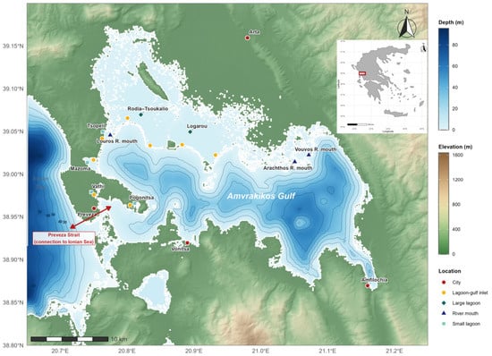
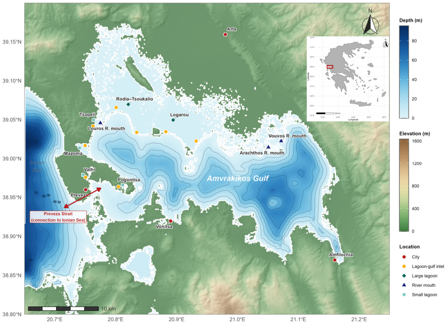
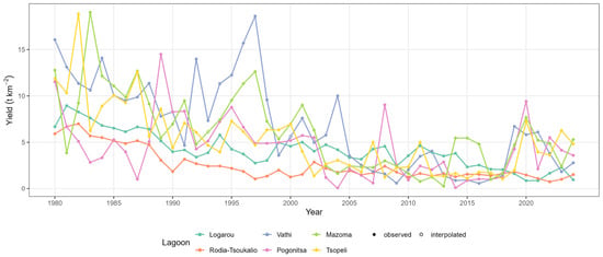
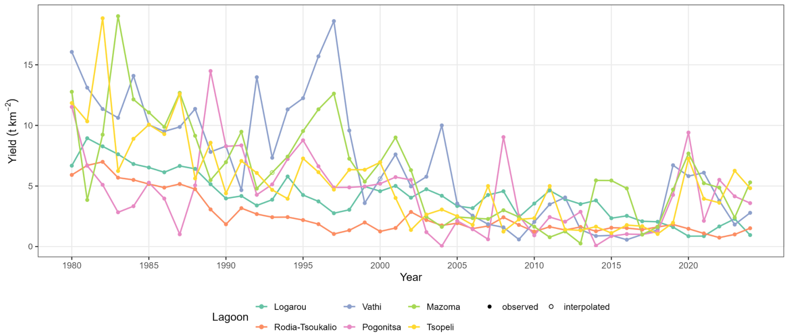
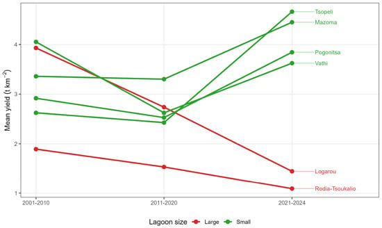
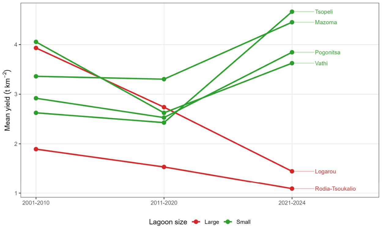
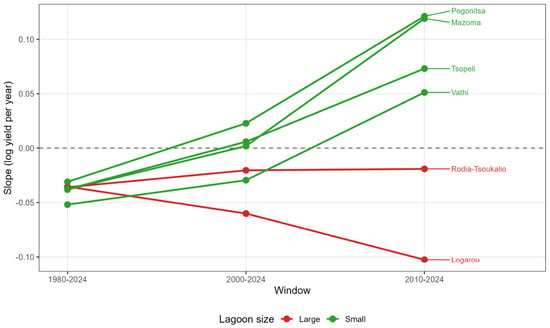
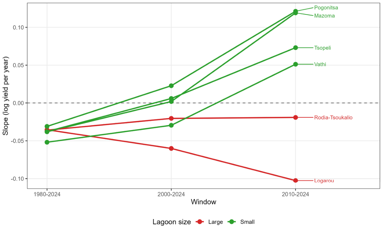
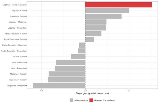
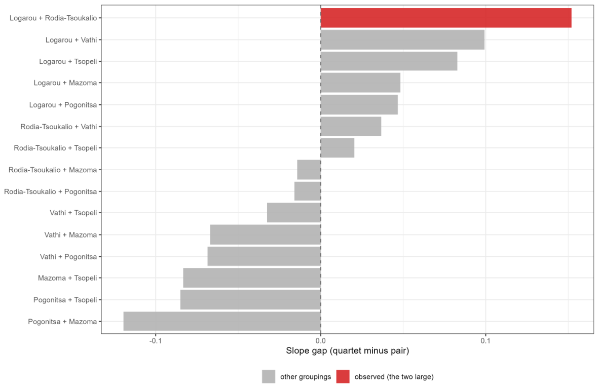
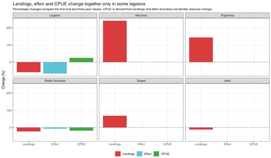
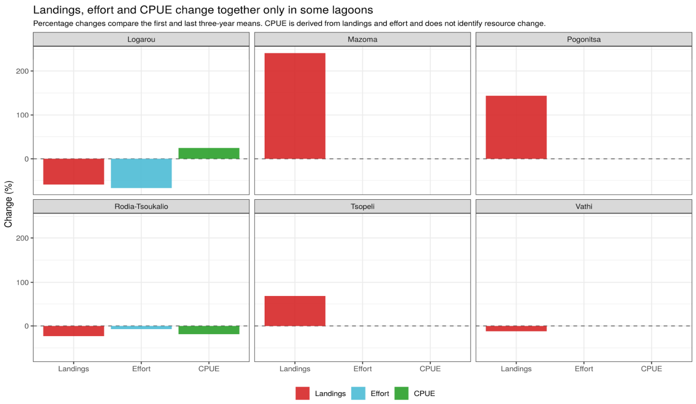
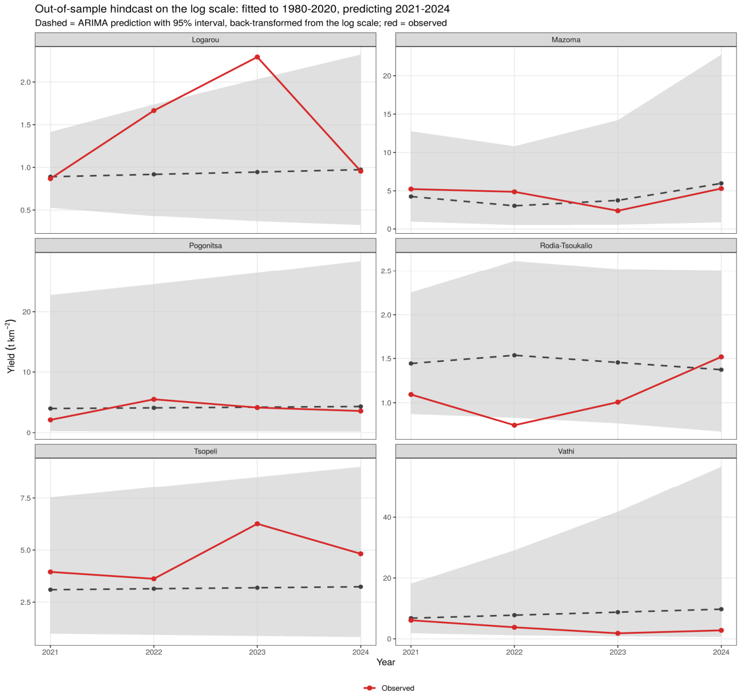

Disclaimer/Publisher’s Note: The statements, opinions and data contained in all publications are solely those of the individual author(s) and contributor(s) and not of MDPI and/or the editor(s). MDPI and/or the editor(s) disclaim responsibility for any injury to people or property resulting from any ideas, methods, instructions or products referred to in the content. |
© 2026 by the authors. Licensee MDPI, Basel, Switzerland. This article is an open access article distributed under the terms and conditions of the Creative Commons Attribution (CC BY) license.