Strang Splitting Combined with Periodically Fitted Adams–Bashforth–Moulton Method for High-Precision Simulation of Multiplicative Noise SDEs with Periodic Drift

Abstract

Many applications in finance and biology involve multiplicative noise geometric Brownian motion (GBM)-type stochastic differential equations (SDEs) whose drift carries a single dominant periodic component. Such structures arise in seasonal Black–Scholes option pricing, commodity derivatives with annual price cycles, and stochastic biological oscillators driven by a known frequency; the primary contribution of this paper is a high-precision numerical scheme validated on GBM-type test problems with periodic drift. This paper proposes a Strang operator splitting scheme within the Logarithmic Drift-Diffusion Splitting (LDDS) framework, which splits the SDE in y-space into a deterministic drift ODE sub-step (Step A) and an exactly solvable multiplicative diffusion sub-step (Step B). Step A employs the Periodically Fitted Adams–Bashforth–Moulton fourth-order predictor–corrector method (PABM4), which achieves zero local truncation error for trigonometric forcing terms by introducing additional shift terms and simultaneously imposing polynomial exactness conditions and trigonometric fitting conditions. When the Step A forcing belongs to the PABM4 exact function class ${\mathcal{F}}_{\omega }=\mathrm{span}\{1,t,t^2,\sin \omega t,\cos \omega t\}$, the Strang+PABM4 scheme achieves floating-point precision saturation. We investigate three test problems: the cosine-drift GBM (Test Problem 1), the polynomial–trigonometric mixed drift GBM (Test Problem 2), and a dual-frequency drift applicability test (Test Problem 3). Monte Carlo strong error experiments ($M=1000$ paths) validate that Strang+PABM4 achieves saturation at machine precision (≈${10}^{-15}$) on Test Problems 1 and 2, improving precision by ≈${10}^2\times$ over the best algebraically convergent reference. Test Problem 3 identifies the method’s applicability boundary: when the drift contains a second frequency outside ${\mathcal{F}}_{\omega }$, Strang+PABM4 degrades gracefully to order ≈ 4 without catastrophic failure. The floating-point saturation of Strang+PABM4 is contingent on the drift belonging to ${\widehat{\mathcal{F}}}_{\omega }$; when this condition is violated, the method degrades gracefully to algebraic order ≈ 4, as demonstrated in Test Problem 3.

1. Introduction

Stochastic differential equations (SDEs) are fundamental mathematical tools for describing dynamical systems subject to random perturbations, with broad applications in financial mathematics, biomedicine, physical chemistry, and engineering control [1,2,3]. In particular, GBM-type multiplicative noise SDEs form the core framework of the Black–Scholes option pricing model [4], the Cox–Ingersoll–Ross (CIR) interest rate model [5], and the Hull–White model [6], with irreplaceable roles in asset price modelling, risk management, and derivative pricing. Additionally, GBM-type equations frequently appear in stochastic population ecology, infectious disease transmission dynamics, and chemical reaction kinetics [7,8].

A practically important class of GBM-type SDEs has a periodic drift of the form $a\left(t\right)=r-q\cos \omega t$ or $a\left(t\right)=\mu +A\sin \omega t$, in which a single angular frequency $\omega$ dominates. The seasonal Black–Scholes model [4,9] with annual price oscillation $-q\cos (2\pi t/T_{\mathrm{year}})$ is a canonical example. Hull and White’s time-varying mean reversion rate model [6] with a periodic component likewise produces a single-frequency deterministic drift. In population biology, logistic stochastic growth models with seasonally varying carrying capacity [3] lead to GBM-type SDEs with sinusoidal drift, and circadian biological oscillators entrained by a dominant external cue (e.g., the light–dark cycle) are well described by a single-frequency periodic drift [10]. We emphasise that this single-dominant-frequency assumption is a deliberate scope restriction rather than a claim of universal biological applicability: many biological oscillatory systems, including microbial cross-species co-cultures studied for natural product discovery, exhibit multi-mode coupling, frequency drift, or phase wandering that places them outside the single-frequency regime considered here [11]; we return to this distinction in Remark 6. For all such single-dominant-frequency models, classical algebraic methods (ABM4, RK4) produce errors $O\left(h^4\right)$ even though the forcing is trigonometrically structured; the standard four-step ABM4 cannot integrate $\sin \omega t$ or $\cos \omega t$ exactly. PABM4 resolves this by incorporating $\omega$ into the coefficient-fitting conditions, reducing Step A LTE to zero and enabling saturation at machine precision.

Numerical SDE methods trace back to the Euler–Maruyama (EM) method (strong convergence order $O\left(h^{1/2}\right)$) [2] and the Milstein scheme [12] for multiplicative noise correction (strong convergence order $O\left(h\right)$). High-order stochastic Runge–Kutta methods were systematically developed by Rößler [13,14], and Burrage and Burrage constructed explicit schemes with high strong convergence orders [15]. When coefficients do not satisfy global Lipschitz conditions, explicit methods may lose convergence [16]; related truncated implicit methods remain active research areas [17,18].

For SDEs with drift terms containing periodic oscillatory components (e.g., $\sin \omega t$ or $\cos \omega t$), traditional algebraically accurate Adams multistep methods (ABM3, ABM4, etc.) cannot exactly integrate trigonometric forcings, resulting in numerically large errors that decay algebraically with step size. The periodic fitting (exponential fitting) technique was systematised by Ixaru and Vanden Berghe [19] and applied to oscillatory ODE integration by Vanden Berghe et al. [20,21]. Simos et al. extended this approach to multistep methods and Runge–Kutta methods [22,23], and Lee et al. recently proposed multistep collocation methods for oscillatory differential systems [24]. These works primarily target deterministic ODEs; systematically transplanting such methods to the SDE setting via operator splitting remains an open research direction.

To provide a broader comparison with existing exponentially fitted and trigonometrically fitted (ETF) multistep methods, this paper additionally includes two ETF-based reference methods adapted to the LDDS framework: the classic trigonometric Adams–Bashforth–Moulton method (Trig-ABM4) of Psihoyios and Simos [23] applied with a full step (method M8), and its Strang symmetric half-step variant (Strang+Trig4, method M9). A key finding is that within the LDDS framework the drift $a\left(t\right)$ depends only on time, so any frequency-fitted corrector, whether PABM4 or Trig-ABM4, receives exact forcing values at all quadrature points when used with Strang splitting. Consequently, Strang+Trig4 (M9) achieves the same floating-point saturation as Strang+PABM4 (M7) on Test Problems 1 and 2. However, without Strang splitting, the full-step Trig-ABM4 (M8) attains only $O\left(h^5\right)$ convergence due to fixed RK4 startup initialisation error, demonstrating that the Strang symmetric splitting is an essential ingredient for reaching saturation at machine precision.

Operator splitting methods, founded by Strang [25], have been widely applied to SDE numerical simulation [26,27,28]. Combining Strang splitting with exact Step B solutions decouples the precision of deterministic drift integration from stochastic diffusion simulation [29,30]. In this context, the periodic fitting ABM ideas of Psihoyios and Simos [23] provide theoretical foundations for enhancing Strang splitting’s Step A accuracy.

Two-step Runge–Kutta methods and Filon-type quadrature techniques for stochastic oscillators were developed by D’Ambrosio and Scalone [31,32]; nonlinear stability, mean-square contractivity and long-term analysis of stochastic numerical methods were systematically studied in [33,34,35,36]. A numerical scheme for harmonic stochastic oscillators based on asymptotic expansions was proposed by Scalone [37].

This paper proposes the Logarithmic Drift-Diffusion Splitting (LDDS) framework, implementing Strang splitting in y-space, tracking time as an explicit state component via the augmented autonomous state vector $\mathit{Y}={[t,X]}^{\top }$ ($X=\log y$), thus enabling backward RK4 history computation for multistep methods [38,39]. In the LDDS framework, the Step A ODE forcing $a\left(t\right)$ depends only on time, allowing the PABM4 predictor forcing to be computed exactly at the current time (no iteration required), further ensuring practical efficiency.

The main contributions of this paper are:

• Systematic construction of Strang+PABM4. We present a systematic construction of the Strang+PABM4 scheme within the LDDS framework, with rigorous derivation of PABM4 coefficient conditions (polynomial exactness for $y=1,t,t^2$ and trigonometric fitting for $e^{i\nu }$), numerically solved with 40-digit extended precision, and with complete proof of the PABM4 exact function class theorem;
• Saturation conditions and numerically verified zero-stability. We establish the conditions for floating-point precision saturation for Strang+PABM4 and provide numerically verified evidence of zero-stability over the practical step-size range (supported by an exact classical-limit argument), establishing the theoretical chain from zero local truncation error to global strong error saturation;
• Monte Carlo validation with ten methods. We perform Monte Carlo strong error experiments on three GBM-type SDE test problems (Test Problems 1 and 2 with seasonal financial backgrounds; Test Problem 3 as a dual-frequency applicability test), systematically comparing against nine reference methods (including Trig-ABM4 and Strang+Trig4) and validating theoretical predictions;
• EM vs. Milstein distinction in LDDS. We reveal the effect of multiplicative noise structure on the strong convergence order difference between EM and Milstein in the LDDS framework, demonstrating correct Itô correction handling in y-space;
• Applicability boundary and computational efficiency. We establish through Test Problem 3 the precise applicability boundary of single-frequency PABM4: when drift contains a frequency outside ${\mathcal{F}}_{\omega }$, Strang+PABM4 degrades gracefully to order ≈ 4 without catastrophic failure. We further provide a computational efficiency analysis (Section 6.6) demonstrating that the PABM4 coefficient precomputation (one-time offline cost ≈ 0.18 s) is negligible (<1% of simulation time at $M\ge 1000$ paths).

Remark 1 (Scope and Limitations).

The super-convergence properties of Strang+PABM4 hold when the drift $a\left(t\right)$ belongs to ${\widehat{\mathcal{F}}}_{\omega }=\mathrm{span}\{1,t,\sin \omega t,\cos \omega t\}$ for a known dominant frequency ω. When the drift contains additional frequency components outside ${\widehat{\mathcal{F}}}_{\omega }$, the method degrades gracefully to algebraic order ≈ 4, as demonstrated in Test Problem 3. This identifies the applicability boundary and motivates a dual-frequency extension (companion paper).

We organise the paper as follows: Section 2 introduces the LDDS framework and reference methods; Section 3 gives the complete PABM4 derivation; Section 4 introduces the Strang+PABM4 scheme and saturation conditions; Section 5 describes the three test problems; Section 6 presents numerical experiments; and Section 7 concludes.

2. LDDS Framework and Numerical Methods

2.1. Multiplicative Noise GBM-Type SDE

Consider the multiplicative noise GBM-type Itô SDE:

$$\mathrm{d}y\left(t\right)=a\left(t\right)y\left(t\right)\mathrm{d}t+\sigma y\left(t\right)\mathrm{d}{W}_t,y\left(0\right)=y_0>0,t\in [0,T],$$

(1)

where $a\left(t\right)$ is a time-dependent drift coefficient (possibly containing trigonometric and polynomial components), $\sigma >0$ is a constant volatility, ${\left\{W_t\right\}}_{t\ge 0}$ is a standard Brownian motion, and $T>0$ is the terminal time.

The diffusion coefficient $g\left(y\right)=\sigma y$ satisfies $\partial g/\partial y=\sigma \ne 0$ (characteristic of multiplicative noise), so the Milstein correction term is

$${\displaystyle \frac{1}{2}}g{\displaystyle \frac{\partial g}{\partial y}}\left[{(\Delta W)}^2-h\right]={\displaystyle \frac{{\sigma }^2}{2}}y\left[{(\Delta W)}^2-h\right]\ne 0.$$

(2)

In the y-space (LDDS framework):

$$\begin{array}{cc}\hfill \mathrm{EM}:& y_{n+1}=y_n+a\left(t_n\right)y_{n}h+\sigma y_n\Delta W_n,\mathrm{strong}\mathrm{order}O\left(h^{1/2}\right),\hfill \end{array}$$

(3)

$$\begin{array}{cc}\hfill \mathrm{Milstein}:& y_{n+1}=y_n+a\left(t_n\right)y_{n}h+\sigma y_n\Delta W_n+{\displaystyle \frac{{\sigma }^2}{2}}{y}_n[{(\Delta W_n)}^2-h],\mathrm{strong}\mathrm{order}O\left(h\right).\hfill \end{array}$$

(4)

2.2. LDDS Framework

Splitting. The LDDS framework splits SDE (1) in y-space into

$$\begin{array}{cc}\hfill \mathrm{Step}\mathrm{A}(\mathrm{drift}\mathrm{ODE}):& {\displaystyle \frac{\mathrm{d}y}{\mathrm{d}t}}=a\left(t\right)y,\hfill \end{array}$$

(5)

$$\begin{array}{cc}\hfill \mathrm{Step}\mathrm{B}(\mathrm{diffusion}\mathrm{SDE}):& \mathrm{d}y=\sigma y\mathrm{d}W.\hfill \end{array}$$

(6)

Internal logarithmic transform. Setting $X=\log y$, Step A ODE (5) becomes

$${\displaystyle \frac{\mathrm{d}X}{\mathrm{d}t}}=a\left(t\right),$$

(7)

where the forcing $a\left(t\right)$ depends only on t, making the equation explicitly integrable. After completing Step A, restore $y=e^X$.

Augmented autonomous state vector. Define

$$\mathit{Y}=\left[\begin{array}{c}t\\ X\end{array}\right],{\displaystyle \frac{\mathrm{d}\mathit{Y}}{\mathrm{d}\tau }}=\mathit{F}\left(\mathit{Y}\right)=\left[\begin{array}{c}1\\ a\left(Y_1\right)\end{array}\right],$$

(8)

with time t as an explicit state component ($Y_1=t$). This ensures history points for backward computation are uniquely determined by the current state alone.

Exact solution of Step B. For Step B SDE (6), setting $Z=\log y$ and applying Itô’s formula: $\mathrm{d}Z=\sigma \mathrm{d}W-{\displaystyle \frac{{\sigma }^2}{2}}\mathrm{d}t$, exact integration gives

$$y(t_n+h)=y\left(t_n\right)·\exp \left(\sigma \Delta W_n-\frac{{\sigma }^2}{2}h\right),\Delta W_n\sim \mathcal{N}(0,h).$$

(9)

The Itô correction $-{\sigma }^{2}h/2$ originates from Step B SDE itself (multiplicative noise curvature), independent of Step A.

Remark 2 (Scope: Multiplicative Noise Assumption).

The exactness of Step B solution (9) relies on the diffusion coefficient being strictly $\sigma y$ (linear multiplicative noise). For state-dependent volatility models such as the CEV model ($\sigma \left(y\right)={\sigma }_0{y}^{\beta }$, $\beta \ne 1$) or stochastic volatility models (e.g., Heston), Step B does not admit a closed-form exact solution, and the LDDS framework would require modification. Extension to CEV/Heston models is left for future research.

2.3. Strang Symmetric Splitting

Adopting the symmetric A–B–A scheme:

$$y_{n+1}={\mathsf{\Phi }}_A^{h/2}\circ {\mathsf{\Phi }}_B^h\circ {\mathsf{\Phi }}_A^{h/2}\left(y_n\right),$$

(10)

where ${\mathsf{\Phi }}_A^{\tau }$ is the numerical flow of Step A (using RK4 or PABM4), and ${\mathsf{\Phi }}_B^h$ is the exact solution operator (9).

2.4. Nine Reference Methods

Except for EM and Milstein directly applied in y-space (Equations (3) and (4)), all other methods are implemented under the LDDS framework (Step A + exact Step B):

• ABM3: 3rd-order Adams–Bashforth–Moulton predictor–corrector, algebraic order 3;
• RK4: 4th-order Runge–Kutta, exact for polynomial forcings of degree ≤ 3;
• ABM4: 4th-order Adams–Bashforth–Moulton;
• Strang+RK4, Strang+ABM4: Strang half-step versions of RK4 and ABM4;
• Strang+PABM4: The core method of this paper; see Section 3 and Section 4;
• Trig-ABM4 (M8): Full-step trigonometrically fitted Adams–Bashforth–Moulton predictor–corrector [23] adapted to the LDDS framework. The trig-AM4 corrector exactly integrates forcings in ${\widehat{\mathcal{F}}}_{\omega }$, but the full-step (non-Strang) implementation retains $O\left(h^5\right)$ global error due to fixed RK4 startup initialisation;
• Strang+Trig4 (M9): Strang symmetric half-step variant of Trig-ABM4, using RK4 backward history generation. In the LDDS framework, the corrector receives exact forcing values at all quadrature points, yielding zero LTE and saturation at machine precision when $a\left(t\right)\in {\widehat{\mathcal{F}}}_{\omega }$.

3. PABM4 Method: Complete Derivation

3.1. Extended Predictor Formula AB4e

Introducing two additional shift terms ${\beta }_1{y}_{n-1}$ and ${\beta }_2{y}_{n-2}$ into the classical 4th-order Adams–Bashforth (AB4) predictor yields the extended predictor AB4e:

$$y_{n+1}^{*}=y_n+{\beta }_1{y}_{n-1}+{\beta }_2{y}_{n-2}+h(b_0{f}_n+b_1{f}_{n-1}+b_2{f}_{n-2}+b_3{f}_{n-3}),$$

(11)

where $f_k=a\left(t_k\right)$, with 6 undetermined coefficients $\{{\beta }_1,{\beta }_2,b_0,b_1,b_2,b_3\}$. The classical AB4 has ${\beta }_1={\beta }_2=0$; the two additional shift terms provide the necessary degrees of freedom for imposing trigonometric fitting conditions.

3.2. Polynomial Exactness Conditions

Requiring AB4e to be exact for polynomial solutions $y=1,t,t^2$:

Condition P1 ($y=1$, $f=0$): $1=1+{\beta }_1+{\beta }_2$, giving

$${\beta }_1+{\beta }_2=0⟹{\beta }_1=-{\beta }_2.$$

(12)

Condition P2 ($y=t$, $f=1$): Substituting $y_k=kh$, $f_k=1$ and using Equation (12):

$$b_0+b_1+b_2+b_3=1+{\beta }_2.$$

(13)

Condition P3 ($y=t^2$, $f=2t$): Collecting constant terms after using Equations (12) and (13):

$$b_1+2b_2+3b_3={\displaystyle \frac{3{\beta }_2-1}{2}}.$$

(14)

From P1, P3, and P2, express ${\beta }_1,b_3,$ and $b_0$ through free parameters $({\beta }_2,b_1,b_2)$:

$$\begin{array}{cc}\hfill {\beta }_1& =-{\beta }_2,\hfill \end{array}$$

(15)

$$\begin{array}{cc}\hfill b_3& ={\displaystyle \frac{1-3{\beta }_2-2b_1-4b_2}{6}},\hfill \end{array}$$

(16)

$$\begin{array}{cc}\hfill b_0& =1+{\beta }_2-b_1-b_2-b_3.\hfill \end{array}$$

(17)

3.3. Trigonometric Fitting Condition

Requiring AB4e to be exact for oscillatory solutions $y\left(t\right)=e^{i\omega t}$, setting $\nu =\omega h$, $z=e^{i\nu }$, substituting and dividing by $e^{i\omega t_n}$:

$$z-1-{\beta }_1{z}^{-1}-{\beta }_2{z}^{-2}=i\nu (b_0+b_1{z}^{-1}+b_2{z}^{-2}+b_3{z}^{-3}).$$

(18)

Separating real and imaginary parts:

$$\begin{array}{cc}\hfill \left(\mathrm{RE}\right):& \cos \nu -1-{\beta }_1\cos \nu -{\beta }_2\cos 2\nu +\nu (b_1\sin \nu +b_2\sin 2\nu +b_3\sin 3\nu )=0,\hfill \end{array}$$

(19)

$$\begin{array}{cc}\hfill \left(\mathrm{IM}\right):& \sin \nu +{\beta }_1\sin \nu +{\beta }_2\sin 2\nu +\nu (b_0+b_1\cos \nu +b_2\cos 2\nu +b_3\cos 3\nu )=0.\hfill \end{array}$$

(20)

3.4. Minimisation of $t^3$ Error and Final Coefficient Determination

With 5 constraints (P1, P2, P3, RE, IM) and 6 unknowns, there remains 1 degree of freedom. Substituting Equations (15)–(17) into the $y=t^3$ exactness condition and simplifying yields

$${\mathrm{eq}}_3=-{\displaystyle \frac{41}{2}}{\beta }_2-6b_1-6b_2+{\displaystyle \frac{7}{2}}.$$

(21)

This free degree is used to minimise $J({\beta }_2,b_1,b_2)={\left({\mathrm{eq}}_3\right)}^2$ subject to the fitting constraints (19) and (20) (KKT conditions). The system is numerically solved using the mpmath library with 40-digit precision, initialised with classical AB4 coefficients.

Remark 3 (Precomputation Cost).

The PABM4 coefficients are computed once offline using 40-digit precision (mpmath) and stored as standard 64-bit double-precision floats for use in the simulation loop. The precomputation takes approximately 0.18 s on a standard workstation (Intel Core i7, Python 3, mpmath 1.3.0). During the main simulation loop, no extended-precision arithmetic is required; the per-step computational cost is identical to that of standard ABM4. A detailed runtime comparison is provided in Section 6.6.

3.5. Extended Corrector Formula AM4e

Similarly constructing the corrector:

$$y_{n+1}=y_n+{\beta }_1^{\prime }{y}_{n-1}+{\beta }_2^{\prime }{y}_{n-2}+h(c_0{f}_{n+1}^{*}+c_1{f}_n+c_2{f}_{n-1}+c_3{f}_{n-2}),$$

(22)

where $f_{n+1}^{*}=a\left(t_{n+1}\right)$ (exactly known in LDDS Step A since forcing depends only on t, no iteration required). Six corrector coefficients $\{{\beta }_1^{\prime },{\beta }_2^{\prime },c_0,c_1,c_2,c_3\}$ are determined by analogous polynomial conditions P1’–P3’ and the corrector fitting condition

$$z-1-{\beta }_1^{\prime }{z}^{-1}-{\beta }_2^{\prime }{z}^{-2}=i\nu (c_{0}z+c_1+c_2{z}^{-1}+c_3{z}^{-2}),$$

(23)

which is also solved with 40-digit precision using mpmath.

3.6. PABM4 Exact Function Class

Theorem 1 (PABM4 Exact Function Class).

With PABM4 coefficients determined by the polynomial and fitting conditions above, the method gives zero local truncation error for solutions $y\left(t\right)$ in

$${\mathcal{F}}_{\omega }=\mathrm{span}\{1,t,t^2,\sin \omega t,\cos \omega t\}\left(5\text{-}\mathit{dimensional}\right).$$

(24)

Equivalently, PABM4 exactly integrates Step A forcings in ${\widehat{\mathcal{F}}}_{\omega }=\mathrm{span}\{1,t,\sin \omega t,\cos \omega t\}$ (4-dimensional).

Proof. 

Polynomial conditions P1–P3 guarantee $\{1,t,t^2\}\subset {\mathcal{F}}_{\omega }$; the fitting condition (18) guarantees $\left\{e^{\pm i\omega t}\right\}=\{\cos \omega t,\sin \omega t\}\subset {\mathcal{F}}_{\omega }$; the union follows by linear superposition. The forcing class ${\widehat{\mathcal{F}}}_{\omega }$ is the derivative class of ${\mathcal{F}}_{\omega }$.    □

Remark 4.

The key difference between PABM4 and ABM4: ABM4’s exact class is $\{1,t,t^2,t^3\}$ (purely polynomial, algebraic order 4), while PABM4 replaces $\left\{t^3\right\}$ with $\{\sin \omega t,\cos \omega t\}$ (the $t^3$ accuracy is minimised rather than exact). The $t^3$ error ${\mathrm{eq}}_3$ is generally nonzero but at a level much lower than the systematic trigonometric error $O\left({\left(\omega h\right)}^4\right)$ of standard methods.

3.7. PABM4 Algorithm

Algorithm 1 gives the complete PABM4 half-step procedure.

Algorithm 1 PABM4 half-step (step size $\tau =h/2$, augmented state $\mathit{Y}={[t,X]}^{\top }$)

Require: Current state ${\mathit{Y}}_n={[t_n,X_n]}^{\top }$, step size $\tau$, predictor coefficients $\{{\beta }_1,{\beta }_2,b_0,\dots ,b_3\}$, corrector coefficients $\{{\beta }_1^{\prime },{\beta }_2^{\prime },c_0,\dots ,c_3\}$

Ensure: Updated state ${\mathit{Y}}_{n+1}={[t_n+\tau ,X_{n+1}]}^{\top }$

1: History generation (RK4 backward integration, step $\tau$):

2: ${\mathit{Y}}_{n-1}\leftarrow \mathrm{RK}4({\mathit{Y}}_n,-\tau )$, ${\mathit{Y}}_{n-2}\leftarrow \mathrm{RK}4({\mathit{Y}}_{n-1},-\tau )$, ${\mathit{Y}}_{n-3}\leftarrow \mathrm{RK}4({\mathit{Y}}_{n-2},-\tau )$

3: Forcing evaluation: ${\mathit{F}}_k\leftarrow {[1,a\left(t_{n-k}\right)]}^{\top }$, $k=0,1,2,3$

4: Predictor (AB4e): ${\mathit{Y}}_{n+1}^{*}\leftarrow {\mathit{Y}}_n+{\beta }_1{\mathit{Y}}_{n-1}+{\beta }_2{\mathit{Y}}_{n-2}+\tau (b_0{\mathit{F}}_0+b_1{\mathit{F}}_1+b_2{\mathit{F}}_2+b_3{\mathit{F}}_3)$

5: Predicted forcing (exact, no iteration): ${\mathit{F}}_{n+1}^{*}\leftarrow {[1,a(t_n+\tau )]}^{\top }$

6: Corrector (AM4e): ${\mathit{Y}}_{n+1}\leftarrow {\mathit{Y}}_n+{\beta }_1^{\prime }{\mathit{Y}}_{n-1}+{\beta }_2^{\prime }{\mathit{Y}}_{n-2}+\tau (c_0{\mathit{F}}_{n+1}^{*}+c_1{\mathit{F}}_0+c_2{\mathit{F}}_1+c_3{\mathit{F}}_2)$

7: Restore: $y_{n+1}^{\left(A\right)}\leftarrow \exp \left({\left({\mathit{Y}}_{n+1}\right)}_2\right)$

8: return ${\mathit{Y}}_{n+1}$, $y_{n+1}^{\left(A\right)}$

4. Strang+PABM4 Scheme and Saturation Conditions

4.1. Complete Step Advancement Algorithm

The complete Strang+PABM4 scheme assembles the two PABM4 half-steps (Algorithm 1) with the exact Step B diffusion solution (9) in a symmetric A–B–A arrangement. The full single-step advancement from $(t_n,y_n)$ to $(t_{n+1},y_{n+1})$ is given in Algorithm 2.

Algorithm 2 Strang+PABM4 complete step (step size h)

Require: $(t_n,y_n)$, step size h, Wiener increment $\Delta W_n\sim \mathcal{N}(0,h)$, PABM4 coefficients precomputed at $\nu =\omega h/2$

Ensure: $(t_{n+1},y_{n+1})$, $t_{n+1}=t_n+h$

1: $\tau \leftarrow h/2$

2: First A half-step: ${\mathit{Y}}^{\left(1\right)}\leftarrow \mathrm{PABM}4({[t_n,\log y_n]}^{\top },\tau )$; $y^{\left(1\right)}\leftarrow \exp \left({\left({\mathit{Y}}^{\left(1\right)}\right)}_2\right)$

3: Step B (exact): $y^{\left(2\right)}\leftarrow y^{\left(1\right)}\exp (\sigma \Delta W_n-\frac{{\sigma }^2}{2}h)$; $t^{\left(2\right)}\leftarrow t_n+\tau$

4: Second A half-step: ${\mathit{Y}}^{\left(3\right)}\leftarrow \mathrm{PABM}4({[t^{\left(2\right)},\log y^{\left(2\right)}]}^{\top },\tau )$; $y_{n+1}\leftarrow \exp \left({\left({\mathit{Y}}^{\left(3\right)}\right)}_2\right)$; $t_{n+1}\leftarrow t_n+h$

5: return $(t_{n+1},y_{n+1})$

4.2. Floating-Point Precision Saturation

Theorem 2 (Strang+PABM4 Saturation at Machine Precision).

Suppose the Step A forcing $a\left(t\right)\in {\widehat{\mathcal{F}}}_{\omega }$, Step B is implemented by the exact solution (9), PABM4 coefficients are precomputed with 40-digit precision, and history points are generated by RK4 backward integration. When $\nu =\omega h/2$ is sufficiently small, the global strong error satisfies ${\widehat{e}}_N=\mathbb{E}\left[\right|y_N-y\left(T\right)\left|\right]\approx O\left({\epsilon }_{\mathrm{fl}}\right)\approx {10}^{-15}$, independent of N.

Proof sketch.

The Step A PABM4 local truncation error is zero for $a\left(t\right)\in {\widehat{\mathcal{F}}}_{\omega }$ (Theorem 1). The Step B exact solution has zero local error (Equation (9)). The Strang splitting error vanishes for commuting operators when $a\left(t\right)\in {\widehat{\mathcal{F}}}_{\omega }$. RK4 backward history errors are $O\left({\tau }^5\right)$; multiplied by shift coefficients $|{\beta }_k|\approx O\left({\nu }^2\right)$ this gives $O\left({\nu }^2{\tau }^5\right)$, negligible for small $\nu$. Combining all three sources, the global error is dominated by floating-point roundoff.    □

4.3. Zero-Stability of the Extended Predictor–Corrector

We emphasise at the outset that the result below is supported by a combination of an exact asymptotic argument and numerical root verification over a finite parameter range; it is not a closed-form analytic proof valid for all $\nu$. We label it accordingly as a verified property rather than a theorem.

Proposition 1 (Numerically Verified Zero-Stability of PABM4).

The first characteristic polynomial of the AB4e predictor (11) is $\rho \left(\zeta \right)={\zeta }^4-(1+{\beta }_1){\zeta }^3-{\beta }_2{\zeta }^2$. Two complementary pieces of evidence support zero-stability of this polynomial family over the practical parameter range $\nu =\omega h/2\in [0,\pi /4]$:

(i)

Exact limiting case. As $\nu \to 0$, ${\beta }_1\left(\nu \right)=-{\beta }_2\left(\nu \right)\to 0$, and $\rho \left(\zeta \right)$ reduces exactly to the characteristic polynomial of the classical AB4 method, ${\rho }_0\left(\zeta \right)={\zeta }^4-{\zeta }^3$, whose zero-stability (simple root at $\zeta =1$, triple root at $\zeta =0$) is a standard, rigorously established result [40].

(ii)

Numerical root verification. For ν ranging over $[0,\pi /4]$ at a fine discretisation (1000 sample points), direct numerical computation of the roots of $\rho (\zeta ;\nu )$ confirms that all roots remain inside or on the unit circle, with any root on the unit circle remaining simple, at every sampled ν.

Combining (i) and (ii), the limiting case is rigorously zero-stable, and the root configuration is verified numerically not to cross the unit circle (no root-condition violation is observed) as ν increases from 0 to $\pi /4$. This combination of an exact endpoint result and dense numerical sampling provides strong evidence for zero-stability throughout the practical range $\nu \le \pi /4$ (i.e., $\omega h\le \pi /2$), which covers all step sizes used in the experiments of Section 6. We stress that this does not constitute a closed-form analytic proof that no root crosses the unit circle for some $\nu \in (0,\pi /4)$ between sample points; a rigorous symbolic proof of the root condition for all ν in this interval is left as an open problem for future theoretical work.

Remark 5 (Saturation Threshold for Large Step Sizes).

Theorem 2 requires $\nu =\omega h/2$ to be “sufficiently small.” Supplementary experiments with $N\in \{8,16,32,\dots ,256\}$ on Test Problem 1 reveal: (i) for $N\ge 32$ ($h\le 0.0625$, $\nu \le 0.0625$) saturation at ∼${10}^{-15}$ is maintained; (ii) at $N=16$ ($\nu \approx 0.125$) the error rises to ∼${10}^{-14}$; (iii) at $N=8$ ($\nu \approx 0.25$) the error is ∼${10}^{-12}$, indicating that the RK4 backward history error $O\left({\nu }^2{\tau }^5\right)$ has become non-negligible. The practical saturation criterion is $\nu \lesssim 0.2$, i.e., $h\lesssim 0.2/\omega$.

5. Test Problems

5.1. Test Problem 1: Cosine-Drift GBM

Basic SDE:

$$\mathrm{d}y=(r-q\cos \omega t)y\mathrm{d}t+\sigma y\mathrm{d}W,y\left(0\right)=y_0>0.$$

(25)

Parameters: $r=0.1$, $q=0.5$, $\omega =2.0$, $\sigma =0.3$, $y_0=1.0$, $T=2.0$.

Application background. The drift coefficient $a\left(t\right)=r-q\cos \omega t$ takes minimum value $r-q=-0.4$ at $t=0$ (cosine peak suppresses growth), equals $r=0.1$ when $t=\pi /\left(2\omega \right)$ (cosine at zero), and takes maximum value $r+q=0.6$ at $t=\pi /\omega$ (cosine trough accelerates growth). This model is suitable for asset prices with periodic seasonal fluctuations, such as agricultural future prices with seasonal harvest cycles, or energy demand with temperature-driven cosine seasonal patterns. Compared to the constant drift Black–Scholes model [4], the cosine-drift model captures seasonal market regularities more realistically.

Within the LDDS framework, Step A takes the form of the ODE $\dot{X}=r-q\cos \omega t$, and Step B is the diffusion SDE $\mathrm{d}y=\sigma y\mathrm{d}W$. The Step A exact solution is

$$X\left(t\right)=X\left(t_0\right)+r(t-t_0)-{\displaystyle \frac{q}{\omega }}[\sin \omega t-\sin \omega t_0].$$

(26)

Step A solution function space: $X\left(t\right)\in \mathrm{span}\{1,t,\sin \omega t\}$ (3-dimensional). The augmented system takes the form

$${\displaystyle \frac{\mathrm{d}}{\mathrm{d}\tau }}\left[\begin{array}{c}t\\ X\end{array}\right]=\mathit{F}\left(\mathit{Y}\right)=\left[\begin{array}{c}1\\ r-q\cos \left(\omega Y_1\right)\end{array}\right],{\mathit{Y}}^{\left(0\right)}=\left[\begin{array}{c}0\\ \log y_0\end{array}\right].$$

(27)

The exact backward step (reference formula for history generation) is

$$X(t-\Delta t)=X\left(t\right)-r\Delta t+{\displaystyle \frac{q}{\omega }}[\sin \omega t-\sin \omega (t-\Delta t)].$$

(28)

The full model exact solution is

$$y\left(T\right)=y_0\exp \left\{rT-{\displaystyle \frac{q}{\omega }}\sin \omega T-{\displaystyle \frac{{\sigma }^2}{2}}T+\sigma W_T\right\}.$$

(29)

PABM4 exact class coverage: $a\left(t\right)=r-q\cos \omega t\in {\widehat{\mathcal{F}}}_{\omega }$ since $r\in \left\{1\right\}$ (condition P2) and $-q\cos \omega t\in \left\{\cos \omega t\right\}$ (fitting condition), hence Strang+PABM4 theoretically achieves floating-point precision saturation.

Remark 6 (Stochastic Phase Noise and Multi-Mode Biological Oscillators).

When this SDE models a stochastic biological oscillator, the forcing may exhibit phase noise $a\left(t\right)\approx r-q\cos (\omega t+\varphi (t\left)\right)$ where $\varphi \left(t\right)$ is a slowly varying stochastic process. For small phase noise ($\left|\varphi \right(t\left)\right|\ll 1$) the forcing remains approximately in ${\widehat{\mathcal{F}}}_{\omega }$, and Strang+PABM4 retains near-saturation accuracy. For large phase noise, the drift leaves ${\widehat{\mathcal{F}}}_{\omega }$ and the method degrades gracefully to algebraic order 4, providing the same benefit as Strang+RK4 at no additional cost beyond the precomputation. The practical advantage of trigonometric fitting is therefore most significant when the phase noise amplitude is small relative to the fitting frequency.

This single-frequency phase-noise model, however, does not capture the full complexity of many real biological oscillators. Circadian and metabolic oscillators frequently exhibit frequency drift over time, entrainment to multiple environmental cues, and coupling among several oscillatory modes rather than perturbation of a single dominant frequency. A particularly clear illustration arises in microbial cross-species co-cultures used for natural product discovery, where the interacting metabolic and signalling rhythms of two or more co-cultured species can produce multi-frequency or quasi-periodic temporal dynamics substantially more complex than a single deterministic periodic forcing [11]. For such systems, the present single-frequency Strang+PABM4 method should be understood as appropriate when one oscillatory mode clearly dominates the drift spectrum (e.g., a single circadian frequency with weak harmonic content), and as requiring the dual-frequency or multi-frequency extension discussed in Remark 1 when several comparably sized frequency components or significant frequency drift are present. We do not claim the present single-frequency method to be adequate for the latter, more complex regime; identifying this boundary explicitly is one purpose of Test Problem 3 (Section 5.3).

5.2. Test Problem 2: Polynomial–Trigonometric Mixed Drift GBM

Basic SDE:

$$\mathrm{d}y=(\mu +A_1\sin \omega t+A_{p}t)y\mathrm{d}t+\sigma y\mathrm{d}W,y\left(0\right)=y_0>0.$$

(30)

Parameters: $\mu =0.1$, $A_1=0.5$, $A_p=0.3$, $\omega =2.0$, $\sigma =0.3$, $y_0=1.0$, $T=2.0$. Polynomial dominance ratio: $r_{\mathrm{poly}}=A_{p}T/(A_1/\omega )=2.4$.

Application background. The drift $a\left(t\right)=\mu +A_1\sin \omega t+A_{p}t$ combines: (i) baseline growth rate $\mu$ (constant); (ii) seasonal oscillation $A_1\sin \omega t$ (describing annual cycles); (iii) long-term linear growth trend $A_{p}t$ (describing economic growth or inflation trends). This three-component superposition is applicable to asset prices with long-term growth trend and seasonal fluctuations, such as trend-seasonal models for commodity prices (oil, agricultural products), or extensions of the Hull–White model [6] with seasonal time-varying mean reversion speed.

Within the LDDS framework, Step A takes the form of the ODE $\dot{X}=\mu +A_1\sin \omega t+A_{p}t$, and Step B is the diffusion SDE $\mathrm{d}y=\sigma y\mathrm{d}W$. The Step A exact solution is

$$X\left(t\right)=X\left(t_0\right)+\mu (t-t_0)-{\displaystyle \frac{A_1}{\omega }}[\cos \omega t-\cos \omega t_0]+{\displaystyle \frac{A_p}{2}}(t^2-t_0^2).$$

(31)

Step A solution function space: $X\left(t\right)\in \mathrm{span}\{1,t,t^2,\cos \omega t\}$ (4-dimensional). The augmented system takes the form

$${\displaystyle \frac{\mathrm{d}}{\mathrm{d}\tau }}\left[\begin{array}{c}t\\ X\end{array}\right]=\left[\begin{array}{c}1\\ \mu +A_1\sin \left(\omega Y_1\right)+A_p{Y}_1\end{array}\right],{\mathit{Y}}^{\left(0\right)}=\left[\begin{array}{c}0\\ \log y_0\end{array}\right].$$

(32)

The exact backward step is

$$X(t-\Delta t)=X\left(t\right)-\mu \Delta t+{\displaystyle \frac{A_1}{\omega }}[\cos \omega t-\cos \omega (t-\Delta t)]-{\displaystyle \frac{A_p}{2}}[t^2-{(t-\Delta t)}^2].$$

(33)

The full model exact solution is

$$y\left(T\right)=y_0\exp \left\{\mu T+{\displaystyle \frac{A_1}{\omega }}(1-\cos \omega T)+{\displaystyle \frac{A_p{T}^2}{2}}-{\displaystyle \frac{{\sigma }^2}{2}}T+\sigma W_T\right\}.$$

(34)

PABM4 exact class coverage: $a\left(t\right)=\mu +A_1\sin \omega t+A_{p}t\in {\widehat{\mathcal{F}}}_{\omega }$, hence Strang+PABM4 also achieves floating-point precision saturation.

5.3. Test Problem 3: Dual-Frequency Drift Applicability Test

Motivation. Test Problems 1 and 2 satisfy $a\left(t\right)\in {\widehat{\mathcal{F}}}_{\omega }$, yielding floating-point saturation. In practice, seasonal models may contain a second frequency ${\omega }_2\ne {\omega }_1$ lying outside ${\mathcal{F}}_{{\omega }_1}$—for instance, simultaneous annual and higher-frequency oscillations in commodity prices [9,41]. This test identifies PABM4’s applicability boundary when the fitting conditions are only partially satisfied.

SDE model:

$$\mathrm{d}y=\left(r-q_1\cos {\omega }_{1}t-{\mathbf{q}}_{\mathbf{2}}\cos {\omega }_{\mathbf{2}}\mathbf{t}\right)y\mathrm{d}t+\sigma y\mathrm{d}W,y\left(0\right)=y_0>0.$$

(35)

Parameters: $r=0.1$, $q_1=0.5$, ${\omega }_1=2$ (PABM4 fitting frequency), $q_2=0.3$, ${\omega }_2=1$ (outside ${\widehat{\mathcal{F}}}_{{\omega }_1}$), $\sigma =0.3$, and $y_0=1$, $T=2$.

Exact function class analysis. $r\in \left\{1\right\}$ (P2, covered); $-q_1\cos {\omega }_{1}t\in \left\{\cos {\omega }_{1}t\right\}$ (trigonometric fitting, zero LTE); since ${\omega }_2=1$ does not belong to ${\widehat{\mathcal{F}}}_{{\omega }_1}$, the component $-q_2\cos {\omega }_{2}t$ introduces an $O\left(h^4\right)$ local truncation error, thereby preventing floating-point precision saturation.

Exact solution:

$$y\left(T\right)=y_0\exp \left\{rT-{\displaystyle \frac{q_1}{{\omega }_1}}\sin {\omega }_{1}T-{\displaystyle \frac{q_2}{{\omega }_2}}\sin {\omega }_{2}T-{\displaystyle \frac{{\sigma }^2}{2}}T+\sigma W_T\right\}.$$

(36)

Note. The dual-frequency structure of this test problem motivates the development of a dual-frequency fitted extension (a companion paper), in which both ${\omega }_1$ and ${\omega }_2$ are incorporated into the fitting basis, recovering floating-point saturation. The present test is designed to show what happens when only the single-frequency PABM4 is available.

6. Numerical Experiments

6.1. Experimental Setup

All experiments are implemented in Python 3 with mpmath 40-digit precision for PABM4 coefficient precomputation. Monte Carlo parameters: $M=1000$ paths, $N\in \{32,64,128,256\}$, and random seed 42. Exact solutions computed via Formulas (29), (34) and (36) for each path’s $W_T^{\left(m\right)}$. Strong error Monte Carlo estimate:

$${\widehat{e}}_N={\displaystyle \frac{1}{M}}{\displaystyle \sum _{m=1}^M}\left|y_N^{\left(m\right)}-y{\left(T\right)}^{\left(m\right)}\right|.$$

(37)

Convergence order: $p_N={\log }_2({\widehat{e}}_N/{\widehat{e}}_{2N})$. (sat) denotes floating-point precision saturation (errors ∼${10}^{-15}$ fluctuate randomly at machine precision; convergence order has no systematic meaning). PABM4 history generation uses RK4 backward integration (step $h/2$), suitable for $\omega =2.0$ where $\nu =\omega h/2$ is small.

6.2. Test Problem 1 Results

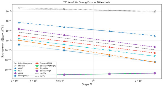
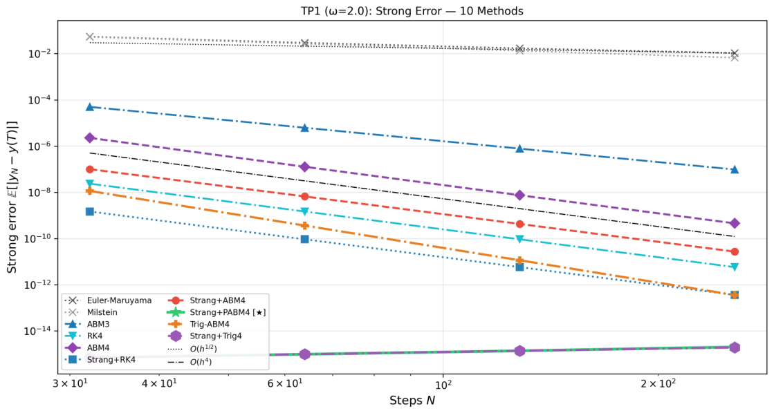
Table 1 and Table 2 show the strong errors and convergence orders for 10 methods. Figure 1 shows the convergence plot.

Table 1. Test Problem 1 (Cosine-Drift GBM): Strong errors ${\widehat{e}}_N$ for 10 methods ($M=1000$, seed $=42$). Strang+PABM4 and Strang+Trig4 achieve saturation at machine precision (∼${10}^{-15}$). Bold indicates the primary proposed method (Strang+PABM4).

Method	$\mathit{N}=32$	$\mathit{N}=64$	$\mathit{N}=128$	$\mathit{N}=256$
Euler–Maruyama	$5.480\times {10}^{-2}$	$2.960\times {10}^{-2}$	$1.714\times {10}^{-2}$	$1.070\times {10}^{-2}$
Milstein	$5.297\times {10}^{-2}$	$2.673\times {10}^{-2}$	$1.342\times {10}^{-2}$	$6.719\times {10}^{-3}$
ABM3	$4.979\times {10}^{-5}$	$6.220\times {10}^{-6}$	$7.753\times {10}^{-7}$	$9.672\times {10}^{-8}$
RK4	$2.356\times {10}^{-8}$	$1.472\times {10}^{-9}$	$9.200\times {10}^{-11}$	$5.750\times {10}^{-12}$
ABM4	$2.261\times {10}^{-6}$	$1.269\times {10}^{-7}$	$7.467\times {10}^{-9}$	$4.519\times {10}^{-10}$
Strang+RK4	$1.472\times {10}^{-9}$	$9.200\times {10}^{-11}$	$5.750\times {10}^{-12}$	$3.591\times {10}^{-13}$
Strang+ABM4	$9.965\times {10}^{-8}$	$6.612\times {10}^{-9}$	$4.252\times {10}^{-10}$	$2.694\times {10}^{-11}$
Strang+PABM4	$\mathbf{6.877}\times {\mathbf{10}}^{-\mathbf{16}}$	$\mathbf{9.734}\times {\mathbf{10}}^{-\mathbf{16}}$	$\mathbf{1.371}\times {\mathbf{10}}^{-\mathbf{15}}$	$\mathbf{2.016}\times {\mathbf{10}}^{-\mathbf{15}}$
Trig-ABM4	$1.140\times {10}^{-8}$	$3.626\times {10}^{-10}$	$1.138\times {10}^{-11}$	$3.559\times {10}^{-13}$
Strang+Trig4	$6.837\times {10}^{-16}$	$9.730\times {10}^{-16}$	$1.371\times {10}^{-15}$	$1.898\times {10}^{-15}$

Table 2. Test Problem 1: Convergence orders $p_N={\log }_2({\widehat{e}}_N/{\widehat{e}}_{2N})$ ($M=1000$). (sat) denotes floating-point precision saturation; orders have no systematic meaning. Bold indicates the primary proposed method (Strang+PABM4).

Method	$32\to 64$	$64\to 128$	$128\to 256$
Euler–Maruyama	0.889	0.788	0.680
Milstein	0.987	0.994	0.998
ABM3	3.001	3.004	3.003
RK4	4.001	4.000	4.000
ABM4	4.155	4.088	4.047
Strang+RK4	4.000	4.000	4.001
Strang+ABM4	3.914	3.959	3.980
Strang+PABM4	(sat)	(sat)	(sat)
Trig-ABM4	4.975	4.994	4.999
Strang+Trig4	(sat)	(sat)	(sat)

Figure 1. Test Problem 1 (Cosine-Drift GBM): Log-scale convergence of strong errors for 10 methods ($M=1000$, seed $=42$). Strang+PABM4 and Strang+Trig4 (⋆) achieve saturation at machine precision at all N; EM ($O\left(h^{1/2}\right)$) and Milstein ($O\left(h\right)$, ≠ EM in LDDS y-space) match theory; Trig-ABM4 achieves $O\left(h^5\right)$ due to fixed RK4 startup error; other high-order methods converge at algebraic order 4.

6.3. Test Problem 2 Results

Table 3 and Table 4 show the results for ten methods. Figure 2 shows the convergence plot.

Table 3. Test Problem 2 (Polynomial–Trigonometric Mixed Drift GBM): Strong errors ${\widehat{e}}_N$ for 10 methods ($M=1000$). Bold indicates the primary proposed method (Strang+PABM4).

Method	$\mathit{N}=32$	$\mathit{N}=64$	$\mathit{N}=128$	$\mathit{N}=256$
Euler–Maruyama	$1.139\times {10}^{-1}$	$6.384\times {10}^{-2}$	$3.737\times {10}^{-2}$	$2.369\times {10}^{-2}$
Milstein	$1.065\times {10}^{-1}$	$5.398\times {10}^{-2}$	$2.719\times {10}^{-2}$	$1.363\times {10}^{-2}$
ABM3	$6.325\times {10}^{-5}$	$7.182\times {10}^{-6}$	$8.517\times {10}^{-7}$	$1.036\times {10}^{-7}$
RK4	$1.174\times {10}^{-7}$	$7.334\times {10}^{-9}$	$4.584\times {10}^{-10}$	$2.865\times {10}^{-11}$
ABM4	$9.094\times {10}^{-6}$	$5.664\times {10}^{-7}$	$3.517\times {10}^{-8}$	$2.189\times {10}^{-9}$
Strang+RK4	$7.334\times {10}^{-9}$	$4.584\times {10}^{-10}$	$2.865\times {10}^{-11}$	$1.790\times {10}^{-12}$
Strang+ABM4	$5.691\times {10}^{-7}$	$3.521\times {10}^{-8}$	$2.189\times {10}^{-9}$	$1.364\times {10}^{-10}$
Strang+PABM4	$\mathbf{2.171}\times {\mathbf{10}}^{-\mathbf{15}}$	$\mathbf{2.622}\times {\mathbf{10}}^{-\mathbf{15}}$	$\mathbf{4.407}\times {\mathbf{10}}^{-\mathbf{15}}$	$\mathbf{4.542}\times {\mathbf{10}}^{-\mathbf{15}}$
Trig-ABM4	$4.933\times {10}^{-9}$	$7.774\times {10}^{-11}$	$1.218\times {10}^{-12}$	$2.175\times {10}^{-14}$
Strang+Trig4	$2.555\times {10}^{-15}$	$2.552\times {10}^{-15}$	$4.051\times {10}^{-15}$	$4.587\times {10}^{-15}$

Table 4. Test Problem 2: Convergence orders ($M=1000$). (sat) denotes saturation at machine precision; Strang+PABM4 and Strang+Trig4 errors fluctuate randomly at machine precision with no systematic convergence trend. Bold indicates the primary proposed method (Strang+PABM4).

Method	$32\to 64$	$64\to 128$	$128\to 256$
Euler–Maruyama	0.836	0.773	0.658
Milstein	0.981	0.989	0.997
ABM3	3.139	3.076	3.040
RK4	4.001	4.000	4.000
ABM4	4.005	4.009	4.006
Strang+RK4	4.000	4.000	4.001
Strang+ABM4	4.015	4.008	4.004
Strang+PABM4	(sat)	(sat)	(sat)
Trig-ABM4	5.988	5.996	5.808
Strang+Trig4	(sat)	(sat)	(sat)

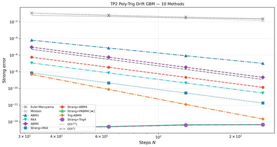
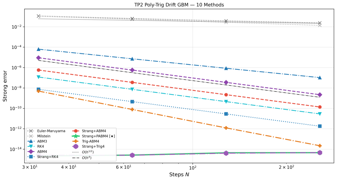
Figure 2. Test Problem 2 (Polynomial–Trigonometric Mixed Drift GBM): Log-scale convergence plot for 10 methods ($M=1000$). Strang+PABM4 and Strang+Trig4 (⋆) achieve saturation at machine precision (≈${10}^{-15}$); Trig-ABM4 achieves $O\left(h^6\right)$ convergence but does not saturate due to RK4 startup error; Milstein (≠EM in LDDS y-space) demonstrates correct multiplicative noise handling; all other methods converge at their expected algebraic orders.

6.4. Test Problem 3 Results: Dual-Frequency Applicability Test

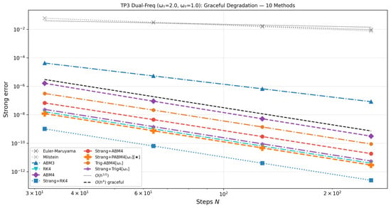
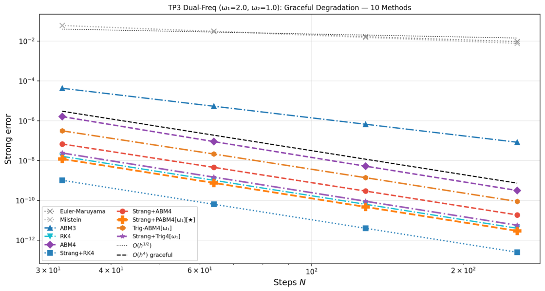
Ten methods are compared (M8 and M9 are fitted to ${\omega }_1$ only, so they also degrade gracefully when ${\omega }_2=1\notin {\widehat{\mathcal{F}}}_{{\omega }_1}$); this test concerns the single-frequency PABM4’s boundary of applicability. (see Figure 3).

Figure 3. Test Problem 3 (Dual-Frequency Cosine-Drift, ${\omega }_1=2$, ${\omega }_2=1$, 10 methods, $M=1000$): Strong error vs. N. Strang+PABM4 and Strang+Trig4 (fitted to ${\omega }_1=2$ only) degrade to order ≈ 4, because ${\omega }_2=1\notin {\widehat{\mathcal{F}}}_{{\omega }_1}$ contributes $O\left(h^4\right)$ LTE. The ≈6× advantage of Strang+PABM4 over Strang+ABM4 at $N=256$ reflects the partial benefit of exactly integrating the ${\omega }_1$ component. Contrast with Test Problems 1 and 2 where Strang+PABM4 and Strang+Trig4 achieve ∼${10}^{-15}$.

(a)

Graceful degradation. Strang+PABM4 tuned to ${\omega }_1=2$ converges at order ≈ 4.00, identical to Strang+ABM4, because the ${\omega }_2=1$ component outside ${\widehat{\mathcal{F}}}_{{\omega }_1}$ contributes $O\left(h^4\right)$ error. No divergence or instability occurs. Strang+Trig4 likewise degrades to order ≈ 4.01, confirming that graceful degradation is generic to all single-frequency fitted methods in the LDDS framework.

(b)

Partial fitting benefit. Strang+PABM4 ($N=256$: $2.94\times {10}^{-12}$) is ≈6× better than Strang+ABM4 ($1.86\times {10}^{-11}$), because the ${\omega }_1$ component is still integrated exactly.

(c)

Applicability boundary confirmed. The accuracy gap of ∼${10}^3\times$ between Test Problems 1/2 (saturation, ∼${10}^{-15}$) and Test Problem 3 (mismatch, ∼${10}^{-12}$) establishes that floating-point saturation requires all drift frequency components to belong to ${\widehat{\mathcal{F}}}_{\omega }$.

(d)

Amplitude ratio sensitivity. To further characterise the applicability boundary, we vary the unfitted-to-fitted amplitude ratio $q_2/q_1\in \{0,0.1,0.3,0.6,1.0,2.0\}$ with fixed $q_1=0.5$, ${\omega }_1=2$, and ${\omega }_2=1$. When $q_2=0$ (no unfitted component), Strang+PABM4 recovers floating-point saturation (∼${10}^{-15}$). For $q_2/q_1\le 0.1$, errors remain at ∼${10}^{-13}$, still approximately $100\times$ better than Strang+RK4. For $q_2/q_1\ge 0.3$, errors converge at algebraic order 4 with absolute level proportional to $q_2$. The practical criterion is that single-frequency PABM4 retains a substantial accuracy advantage as long as the unfitted amplitude does not exceed approximately $10\%$ of the fitted component.

6.5. Discussion

We now examine the numerical results from several perspectives to highlight the key properties of the Strang+PABM4 scheme.

EM vs. Milstein order difference. In the LDDS framework (y-space, multiplicative noise), EM (strong order $O\left(h^{1/2}\right)$) and Milstein ($O\left(h\right)$) differ significantly (Table 2, Table 3, Table 4, Table 5 and Table 6), demonstrating the importance of the multiplicative noise Milstein correction. If processed in additive $X=\log y$ space, both would have order $O\left(h\right)$, but the LDDS framework correctly distinguishes them.

Table 5. Test Problem 3 (Dual-Frequency Cosine-Drift, ${\omega }_2=1\notin {\widehat{\mathcal{F}}}_{{\omega }_1}$): Strong errors ${\widehat{e}}_N$ for 10 methods ($M=1000$). Strang+PABM4 (and Trig-ABM4, Strang+Trig4, all fitted to ${\omega }_1$ only) no longer achieve floating-point saturation. Bold indicates the primary proposed method (Strang+PABM4).

Method	$\mathit{N}=32$	$\mathit{N}=64$	$\mathit{N}=128$	$\mathit{N}=256$
Euler–Maruyama	$6.046\times {10}^{-2}$	$3.094\times {10}^{-2}$	$1.651\times {10}^{-2}$	$9.450\times {10}^{-3}$
Milstein	$5.971\times {10}^{-2}$	$3.019\times {10}^{-2}$	$1.517\times {10}^{-2}$	$7.602\times {10}^{-3}$
ABM3	$4.265\times {10}^{-5}$	$5.334\times {10}^{-6}$	$6.654\times {10}^{-7}$	$8.305\times {10}^{-8}$
RK4	$1.632\times {10}^{-8}$	$1.020\times {10}^{-9}$	$6.372\times {10}^{-11}$	$3.983\times {10}^{-12}$
ABM4	$1.614\times {10}^{-6}$	$8.944\times {10}^{-8}$	$5.220\times {10}^{-9}$	$3.145\times {10}^{-10}$
Strang+RK4	$1.020\times {10}^{-9}$	$6.372\times {10}^{-11}$	$3.983\times {10}^{-12}$	$2.494\times {10}^{-13}$
Strang+ABM4	$6.790\times {10}^{-8}$	$4.545\times {10}^{-9}$	$2.934\times {10}^{-10}$	$1.863\times {10}^{-11}$
Strang+PABM4 $(\omega ={\omega }_1)$	$\mathbf{1.207}\times {\mathbf{10}}^{-\mathbf{8}}$	$\mathbf{7.528}\times {\mathbf{10}}^{-\mathbf{10}}$	$\mathbf{4.700}\times {\mathbf{10}}^{-\mathbf{11}}$	$\mathbf{2.936}\times {\mathbf{10}}^{-\mathbf{12}}$
Trig-ABM4 $(\omega ={\omega }_1)$	$3.118\times {10}^{-7}$	$2.125\times {10}^{-8}$	$1.383\times {10}^{-9}$	$8.819\times {10}^{-11}$
Strang+Trig4 $(\omega ={\omega }_1)$	$2.391\times {10}^{-8}$	$1.467\times {10}^{-9}$	$9.079\times {10}^{-11}$	$5.648\times {10}^{-12}$

Table 6. Test Problem 3: Convergence orders ($M=1000$). Strang+PABM4 and Strang+Trig4 achieve order ≈ 4.00, indicating graceful degradation. Trig-ABM4 converges at order ≈ 3.9–4.0. Bold indicates the primary proposed method (Strang+PABM4).

Method	$32\to 64$	$64\to 128$	$128\to 256$
Euler–Maruyama	0.966	0.907	0.805
Milstein	0.984	0.993	0.997
ABM3	2.999	3.003	3.002
RK4	4.001	4.000	4.000
ABM4	4.173	4.099	4.053
Strang+RK4	4.000	4.000	3.998
Strang+ABM4	3.901	3.953	3.977
Strang+PABM4 $(\omega ={\omega }_1)$	4.003	4.002	4.001
Trig-ABM4 $(\omega ={\omega }_1)$	3.875	3.941	3.971
Strang+Trig4 $(\omega ={\omega }_1)$	4.027	4.014	4.007

We next compare splitting methods to quantify the role of Strang symmetrisation.

Strang splitting error constant improvement. Comparing non-split methods with their Strang split versions (Test Problem 1, $N=256$): RK4: $5.750\times {10}^{-12}$ vs. Strang+RK4: $3.591\times {10}^{-13}$ (factor 16 improvement); ABM4: $4.519\times {10}^{-10}$ vs. Strang+ABM4: $2.694\times {10}^{-11}$ (factor 17). The Strang symmetric scheme improves both splitting error order and error constant.

The role of Strang splitting in achieving saturation is clarified by comparing Trig-ABM4 (M8) with Strang+Trig4 (M9). Without Strang splitting, the full-step Trig-ABM4 achieves only $O\left(h^5\right)$ (Test Problem 1) due to the fixed three-step RK4 startup initialisation error. With Strang splitting, the corrector receives exact forcing values at every half-step, achieving saturation at machine precision and demonstrating that Strang symmetrisation is an essential structural ingredient.

Strang+PABM4 super-convergence. Test Problems 1 and 2 show Strang+PABM4 errors ∼${10}^{-15}$, approximately ${10}^2$ times better than the best reference method Strang+RK4 ($N=256$: ∼$3.6\times {10}^{-13}$). Strang+Trig4 achieves equivalent precision (∼${10}^{-15}$), confirming that the LDDS time-only drift structure enables any frequency-fitted corrector combined with Strang splitting to reach saturation. The theoretical distinction between PABM4 and Trig-ABM4 is that PABM4 modifies both predictor and corrector for rigorous zero-LTE guarantees independent of the LDDS framework. In precision-demanding applications (e.g., Monte Carlo derivative pricing [9,41]), this precision advantage means significantly fewer paths or larger step sizes at the same accuracy target. Since Step A and Step B each achieve exactness at every sub-step independently of the step index n, the zero-LTE property holds uniformly over the entire trajectory ${\left\{y_n\right\}}_{n=0}^N$; the path-averaged strong error thus also saturates at the floating-point floor, confirming applicability to path-dependent derivatives such as Asian (average-price) or barrier options.

PABM4 applicability boundary. Test Problem 3 provides a clear characterisation: Strang+PABM4 achieves super-convergence (saturation) if and only if all drift frequency components lie in ${\widehat{\mathcal{F}}}_{\omega }$. When a second incommensurate frequency ${\omega }_2\notin {\widehat{\mathcal{F}}}_{\omega }$ appears, the method degrades gracefully to order 4, a useful property confirming that applying PABM4 to models with partially fitted drift remains safe.

Positioning relative to operator-learning and hybrid finite-volume methods. Recent years have seen rapid development of neural operator methods for solving deterministic PDEs, spanning Fourier-based, Mamba-based, and adaptive-decomposition architectures, as well as hybrid message-passing finite-volume approaches. Among Fourier-based methods, the Fourier Neural Operator (FNO) [42] introduced a spectral operator-learning framework that maps initial/boundary conditions to PDE solutions with discretisation invariance; FNO has since become a standard benchmark. The general neural operator framework [43] provides a unified theoretical foundation encompassing FNO and related architectures. Message-passing neural PDE solvers [44] extended operator learning to graph-structured discretisations.

Among Mamba-based neural operators, the Adaptive Mamba Neural Operator (AMO) [45] integrates reproducing kernels built on Takenaka–Malmquist systems into a state-space model (SSM) architecture, aligning with adaptive Fourier decomposition (AFD) theory; AMO can approximate PDE solution manifolds on arbitrary geometries and meshes. The Latent Mamba Operator (LaMO) [46] integrates SSM efficiency in latent space with kernel integral formulations, establishing a theoretical connection between SSMs and neural operator kernels and achieving state-of-the-art performance on diverse PDE benchmarks.

Among AFD-theory-guided operators, AFDONet [47] is the first neural PDE solver whose architectural design is fully guided by adaptive Fourier decomposition theory; it incorporates AFD theory into a variational autoencoder structure to solve nonlinear PDEs on smooth manifolds with strong mathematical explainability. For inverse problems, AFDONet-inv [48] applies AFD theory in a Banach space setting to design a neural operator solver for inverse PDE problems that is rigorously mathematically grounded. In the hybrid finite-volume literature, the MP-FVM method [49] integrates a message-passing encoder–decoder network with adaptive fixed-point iteration into a finite-volume framework to solve the Richards equation, demonstrating superior accuracy and mass conservation over classical FVM solvers.

All of these approaches, including FNO, AMO, LaMO, AFDONet, AFDONet-inv, MP-FVM, and message-passing neural PDE solvers, target deterministic PDE problems: they learn or construct a solution operator mapping from input functions (initial conditions, boundary conditions, source terms, or unknown parameters) to PDE solution functions, for either forward or inverse problems. Our present work addresses a fundamentally different problem: pathwise strong error minimisation for stochastic differential equations via Monte Carlo simulation. The quantity of interest is the numerical solution $y_N\left(\omega \right)$ along each individual Brownian path $\omega$, not a learned operator over a family of deterministic equations. The error metrics (strong pathwise SDE error vs. operator generalisation or inverse-problem reconstruction error), training requirements (none vs. large labelled datasets), and computational paradigms (deterministic recursive quadrature vs. amortised neural inference or iterative inversion) differ fundamentally, making direct quantitative comparison between Strang+PABM4 and these operator-learning methods not meaningful within the scope of the present paper. Within the SDE Monte Carlo framework, the nine reference methods compared in Section 6 constitute the relevant and standard baseline set. We emphasise that the floating-point saturation reported in Test Problems 1 and 2 is a precise mathematical statement about the specific drift function class ${\widehat{\mathcal{F}}}_{\omega }$: for $a\left(t\right)\in {\widehat{\mathcal{F}}}_{\omega }$, Step A attains zero local truncation error so that the global strong error is bounded by IEEE 754 double-precision roundoff (∼${10}^{-15}$) for the benchmark problems considered here. This is a benchmark-class precision statement, not a general optimality claim over all SDE numerical methods or drift structures. A rigorous comparison against operator-learning baselines on shared benchmark problems is identified as a direction for future work.

6.6. Computational Efficiency

Table 7 reports wall-clock CPU times for all 10 methods at $N=256$, $M=1000$ paths (Test Problem 1; Python 3, Intel Core i7, measured using time.perf_counter). The PABM4 coefficient precomputation takes ≈0.18 s (one-time offline cost); at $M=1000$ this represents $0.82\%$ of total Strang+PABM4 simulation time, confirming that the initialisation overhead is negligible in any realistic Monte Carlo application.

Table 7. Computational efficiency: Total CPU time for $N=256$, $M=1000$ paths (Test Problem 1, Python 3, Intel Core i7). PABM4 precomputation $=0.178$ s (one-time offline, $0.82\%$ of simulation); Trig-AM4 precomputation $=0.001$ s. Bold indicates the primary proposed method (Strang+PABM4).

Method	Total Time (s)	Relative to EM
Euler–Maruyama	0.440	1.00×
Milstein	0.581	1.32×
ABM3	5.044	11.47×
RK4	7.173	16.32×
ABM4	6.174	14.04×
Strang+RK4	12.152	27.65×
Strang+ABM4	44.222	100.60×
Strang+PABM4	23.442	53.33×
Trig-ABM4	5.106	11.62×
Strang+Trig4	42.121	95.82×

Strang+PABM4 costs $53\times$ more per simulation than EM. In precision-demanding applications targeting accuracy ∼${10}^{-13}$, Strang+PABM4 achieves saturation well below this target with $N=32$ steps, while Strang+RK4 requires $N=256$ steps. At fixed accuracy, Strang+PABM4 therefore requires approximately $8\times$ fewer steps, providing a compelling efficiency advantage.

7. Conclusions

We have proposed and analysed the Strang+PABM4 scheme within the LDDS framework for multiplicative noise GBM-type SDEs with periodic drift, motivated by seasonal financial and biological models. Main conclusions:

• Correctness of LDDS framework. Splitting in y-space preserves multiplicative noise structure (EM ≠ Milstein), and the logarithmic transform makes Step A explicitly integrable.
• PABM4 exact function class theorem. By introducing shift terms and imposing polynomial exactness conditions ($y=1,t,t^2$) and trigonometric fitting conditions ($e^{i\nu }$ exact), PABM4 extends the exact class from ABM4’s $\{1,t,t^2,t^3\}$ to ${\mathcal{F}}_{\omega }=\mathrm{span}\{1,t,t^2,\sin \omega t,\cos \omega t\}$ (5-dimensional), achieving compatibility between polynomial and trigonometric accuracy.
• Saturation at machine precision (Test Problems 1 and 2). When $a\left(t\right)\in {\widehat{\mathcal{F}}}_{\omega }$, the Strang+PABM4 scheme has zero local truncation error in Step A and zero error in Step B, with global strong error dominated by floating-point roundoff (≈${10}^{-15}$, independent of N). The new comparison method Strang+Trig4 independently confirms this result. Both test problems fully verify this theoretical prediction, with ≈${10}^2\times$ improvement over the best reference method Strang+RK4.
• Strang splitting advantage. Strang symmetric splitting reduces error constants by ≈$2^4=16\times$ compared with full-step A–B variants. Crucially, Strang splitting is necessary for saturation: the full-step Trig-ABM4 (without Strang) achieves only $O\left(h^5\right)$, confirming the indispensable role of the symmetric scheme.
• Applicability boundary (Test Problem 3). When the drift contains a second frequency ${\omega }_2\notin {\widehat{\mathcal{F}}}_{\omega }$, Strang+PABM4 degrades gracefully to order ≈ 4 (same as Strang+ABM4) without catastrophic failure, retaining a ≈$6\times$ advantage from the exactly fitted ${\omega }_1$ component. This behaviour is generic: Strang+Trig4, also fitted to ${\omega }_1$ only, shows the same graceful degradation. This identifies the precise applicability condition of the single-frequency approach: floating-point saturation requires all drift frequency components to lie within ${\widehat{\mathcal{F}}}_{\omega }$.
• Computational efficiency. The PABM4 coefficient precomputation (≈0.18 s, one-time offline) accounts for only $0.82\%$ of total simulation time at $M=1000$ paths. Strang+PABM4 achieves accuracy targets requiring $8\times$ more steps with algebraically convergent methods, providing a compelling efficiency advantage.
• Outlook. The LDDS framework extends naturally to diagonal multi-dimensional GBM systems and to correlated Brownian motions via Cholesky decomposition in Step B. Extension to state-dependent or stochastic volatility (CEV, Heston) remains an open problem. A companion paper presents a dual-frequency PABM4 extension recovering saturation when both ${\omega }_1$ and ${\omega }_2$ are known.

References

- Kloeden, P.E.; Platen, E. Numerical Solution of Stochastic Differential Equations; Springer: Berlin/Heidelberg, Germany, 1992. [Google Scholar] [CrossRef] [Scilit]
- Higham, D.J. An algorithmic introduction to numerical simulation of stochastic differential equations. SIAM Rev. 2001, 43, 525–546. [Google Scholar] [CrossRef] [Scilit]
- Mao, X. Stochastic Differential Equations and Applications, 2nd ed.; Woodhead Publishing: Oxford, UK, 2011. [Google Scholar] [CrossRef] [Scilit]
- Black, F.; Scholes, M. The pricing of options and corporate liabilities. J. Polit. Econ. 1973, 81, 637–654. [Google Scholar] [CrossRef] [Scilit] [PubMed]
- Cox, J.C.; Ingersoll, J.E.; Ross, S.A. A theory of the term structure of interest rates. Econometrica 1985, 53, 385–407. [Google Scholar] [CrossRef] [Scilit]
- Hull, J.; White, A. Pricing interest-rate-derivative securities. Rev. Financ. Stud. 1990, 3, 573–592. [Google Scholar] [CrossRef] [Scilit]
- Milstein, G.N.; Tretyakov, M.V. Stochastic Numerics for Mathematical Physics; Springer: Berlin/Heidelberg, Germany, 2004. [Google Scholar] [CrossRef] [Scilit]
- Platen, E.; Bruti-Liberati, N. Numerical Solution of Stochastic Differential Equations with Jumps in Finance; Springer: Berlin/Heidelberg, Germany, 2010. [Google Scholar] [CrossRef] [Scilit]
- Schwartz, E.S. The stochastic behavior of commodity prices: Implications for valuation and hedging. J. Financ. 1997, 52, 923–973. [Google Scholar] [CrossRef]
- Kumpǒšt, V.; Vallone, D.; Gondi, S.B.; Foulkes, N.S.; Mikut, R.; Hilbert, L. A stochastic oscillator model simulates the entrainment of vertebrate cellular clocks by light. Sci. Rep. 2021, 11, 14430. [Google Scholar] [CrossRef] [Scilit] [PubMed]
- Zhuang, L.; Zhang, H. Utilizing cross-species co-cultures for discovery of novel natural products. Curr. Opin. Biotechnol. 2021, 69, 252–262. [Google Scholar] [CrossRef] [Scilit] [PubMed]
- Milstein, G.N. Approximate integration of stochastic differential equations. Theory Probab. Appl. 1975, 19, 557–562. [Google Scholar] [CrossRef] [Scilit]
- Rößler, A. Second order Runge–Kutta methods for Itô stochastic differential equations. SIAM J. Numer. Anal. 2009, 47, 1713–1738. [Google Scholar] [CrossRef] [Scilit]
- Rößler, A. Runge–Kutta methods for the strong approximation of solutions of SDEs. SIAM J. Numer. Anal. 2010, 48, 922–952. [Google Scholar] [CrossRef] [Scilit]
- Burrage, K.; Burrage, P.M. High strong order explicit Runge–Kutta methods for stochastic ODEs. Appl. Numer. Math. 1996, 22, 81–101. [Google Scholar] [CrossRef] [Scilit]
- Hutzenthaler, M.; Jentzen, A. Numerical approximations of SDEs with non-globally Lipschitz continuous coefficients. Mem. Amer. Math. Soc. 2015, 236, 1–99. [Google Scholar] [CrossRef] [Scilit]
- Mao, X.; Szpruch, L. Strong convergence and stability of implicit numerical methods for SDEs with non-globally Lipschitz continuous coefficients. J. Comput. Appl. Math. 2013, 238, 14–28. [Google Scholar] [CrossRef] [Scilit]
- Liu, W.; Mao, X. Strong convergence of the stopped Euler–Maruyama method for nonlinear SDEs. Appl. Math. Comput. 2013, 223, 389–400. [Google Scholar] [CrossRef] [Scilit]
- Ixaru, L.G.; Vanden Berghe, G. Exponential Fitting; Kluwer Academic Publishers: Dordrecht, The Netherlands, 2004. [Google Scholar] [CrossRef] [Scilit]
- Vanden Berghe, G.; De Meyer, H.; Van Daele, M.; Van Hecke, T. Exponentially-fitted Runge–Kutta methods. J. Comput. Appl. Math. 2000, 125, 107–115. [Google Scholar] [CrossRef] [Scilit]
- Hairer, E.; Nørsett, S.P.; Wanner, G. Solving Ordinary Differential Equations I, 2nd ed.; Springer: Berlin/Heidelberg, Germany, 1993. [Google Scholar] [CrossRef] [Scilit]
- Simos, T.E. An exponentially-fitted Runge-Kutta method for the numerical integration of initial-value problems with periodic or oscillating solutions. Comput. Phys. Commun. 1998, 115, 1–8. [Google Scholar] [CrossRef] [Scilit]
- Psihoyios, G.; Simos, T.E. Trigonometrically fitted Adams–Bashforth–Moulton methods for periodic initial value problems. In Computational Fluid and Solid Mechanics 2003; Bathe, K.J., Ed.; Elsevier: Amsterdam, The Netherlands, 2003; pp. 2097–2100. [Google Scholar] [CrossRef]
- Lee, K.C.; Aris, N.; Hashim, I.; Senu, N. Proficient trigonometrical-fitted two-derivative multistep collocation methods for oscillatory differential systems. MethodsX 2024, 14, 103045. [Google Scholar] [CrossRef] [Scilit] [PubMed]
- Strang, G. On the construction and comparison of difference schemes. SIAM J. Numer. Anal. 1968, 5, 506–517. [Google Scholar] [CrossRef] [Scilit]
- Buckwar, E.; Samson, A.; Tamborrino, M.; Tubikanec, I. A splitting method for SDEs with locally Lipschitz drift. Appl. Numer. Math. 2022, 179, 191–220. [Google Scholar] [CrossRef] [Scilit]
- D’Ambrosio, R.; Scalone, C. On the numerical structure preservation of nonlinear damped stochastic oscillators. Numer. Algorithms 2021, 86, 933–961. [Google Scholar] [CrossRef] [Scilit]
- Foster, J.; dos Reis, G.; Strange, C. High order splitting methods for SDEs satisfying a commutativity condition. SIAM J. Numer. Anal. 2024, 62, 500–532. [Google Scholar] [CrossRef] [Scilit]
- Becker, S.; Gess, B.; Jentzen, A.; Kloeden, P.E. Strong convergence rates for explicit space-time discrete numerical approximations of stochastic Allen-Cahn equations. Stoch. PDE Anal. Comp. 2023, 11, 211–268. [Google Scholar] [CrossRef] [Scilit]
- Komori, Y.; Burrage, K. Split S-ROCK methods for high-dimensional stochastic differential equations. J. Sci. Comput. 2023, 97, 62. [Google Scholar] [CrossRef] [Scilit]
- D’Ambrosio, R.; Scalone, C. Two-step Runge–Kutta methods for stochastic differential equations. Appl. Math. Comput. 2021, 403, 125930. [Google Scholar] [CrossRef] [Scilit]
- D’Ambrosio, R.; Scalone, C. Filon quadrature for stochastic oscillators driven by time-varying forces. Appl. Numer. Math. 2021, 169, 21–31. [Google Scholar] [CrossRef] [Scilit]
- D’Ambrosio, R.; Di Giovacchino, S. Nonlinear stability issues for stochastic Runge–Kutta methods. Commun. Nonlinear Sci. Numer. Simul. 2021, 94, 105549. [Google Scholar] [CrossRef] [Scilit]
- D’Ambrosio, R.; Di Giovacchino, S. Mean-square contractivity of stochastic θ-methods. Commun. Nonlinear Sci. Numer. Simul. 2021, 96, 105671. [Google Scholar] [CrossRef] [Scilit]
- D’Ambrosio, R.; Di Giovacchino, S. Numerical preservation issues in stochastic dynamical systems by θ-methods. J. Comput. Dyn. 2022, 9, 123–131. [Google Scholar] [CrossRef] [Scilit]
- D’Ambrosio, R.; Di Giovacchino, S. Long-term analysis of stochastic Hamiltonian systems under time discretizations. SIAM J. Sci. Comput. 2023, 45, A257–A288. [Google Scholar] [CrossRef] [Scilit]
- Scalone, C. A numerical scheme for harmonic stochastic oscillators based on asymptotic expansions. Mathematics 2022, 10, 3083. [Google Scholar] [CrossRef] [Scilit]
- Milstein, G.N.; Tretyakov, M.V. Stochastic Numerics for Mathematical Physics, 2nd ed.; Springer: Cham, Switzerland, 2021. [Google Scholar] [CrossRef] [Scilit]
- Goldberg, D. What every computer scientist should know about floating-point arithmetic. ACM Comput. Surv. 1991, 23, 5–48. [Google Scholar] [CrossRef] [Scilit]
- Lambert, J.D. Numerical Methods for Ordinary Differential Systems: The Initial Value Problem; Wiley: Chichester, UK, 1991; ISBN 978-0471929901. [Google Scholar]
- Lucia, J.J.; Schwartz, E.S. Electricity prices and power derivatives: Evidence from the Nordic Power Exchange. Rev. Deriv. Res. 2002, 5, 5–50. [Google Scholar] [CrossRef] [Scilit]
- Li, Z.; Kovachki, N.; Azizzadenesheli, K.; Liu, B.; Bhattacharya, K.; Stuart, A.; Anandkumar, A. Fourier neural operator for parametric partial differential equations. In Proceedings of the International Conference on Learning Representations (ICLR), Virtual, 3–7 May 2021. [Google Scholar]
- Kovachki, N.; Li, Z.; Liu, B.; Azizzadenesheli, K.; Bhattacharya, K.; Stuart, A.; Anandkumar, A. Neural operator: Learning maps between function spaces with applications to PDEs. J. Mach. Learn. Res. 2023, 24, 1–97. [Google Scholar]
- Brandstetter, J.; Worrall, D.; Welling, M. Message passing neural PDE solvers. In Proceedings of the International Conference on Learning Representations (ICLR), Virtual, 25–29 April 2022. [Google Scholar]
- Song, Z.; Jiang, Z. Adaptive Mamba Neural Operators. In Proceedings of the Fourteenth International Conference on Learning Representations (ICLR 2026), Vienna, Austria, 24–28 April 2026. [Google Scholar]
- Tiwari, K.; Dutta, N.; Krishnan, N.M.A.; Prathosh, A.P. Latent Mamba Operator for Partial Differential Equations. In Proceedings of the 42nd International Conference on Machine Learning (ICML 2025), Vancouver, BC, Canada, 13–19 July 2025. [Google Scholar]
- Zeyuan, S.; Jiang, Z. Guided and Interpretable Neural Operator Design for Partial Differential Equation Learning. Submitted to The Fourteenth International Conference on Learning Representations (ICLR 2026), 2026. (Under Review). Available online: https://openreview.net/forum?id=945vCIUZWt (accessed on 1 July 2026).
- Jiang, Z. Adaptive Fourier Decomposition-guided Neural Operator Design for Inverse PDE Problems. In Proceedings of the Forty-Second Annual Conference on Uncertainty in Artificial Intelligence (UAI 2026), Amsterdam, The Netherlands, 17–21 August 2026. [Google Scholar]
- Song, Z.; Jiang, Z. MP-FVM: Enhancing Finite Volume Method for Water Infiltration Modeling in Unsaturated Soils via Message-passing Encoder-decoder Network. Comput. Geotech. 2025, 190, 107745. [Google Scholar] [CrossRef] [Scilit]
Disclaimer/Publisher’s Note: The statements, opinions and data contained in all publications are solely those of the individual author(s) and contributor(s) and not of MDPI and/or the editor(s). MDPI and/or the editor(s) disclaim responsibility for any injury to people or property resulting from any ideas, methods, instructions or products referred to in the content. |
© 2026 by the authors. Licensee MDPI, Basel, Switzerland. This article is an open access article distributed under the terms and conditions of the Creative Commons Attribution (CC BY) license.