


Abstract
The complex and heterogeneous nature of cancer necessitates advanced modeling techniques to better understand tumor dynamics and inform treatment strategies. This paper explores the application of stochastic modeling in cancer research, focusing on five key areas: tumor growth kinetics, evolutionary dynamics of cancer, treatment response and resistance, spatial modeling of tumor progression, and clinical applications of stochastic models. We first examine how stochastic models capture the randomness in tumor growth and proliferation, providing insights into cellular behaviors that deterministic models may overlook. Next, we investigate the evolutionary dynamics that govern tumor heterogeneity and the emergence of resistance, highlighting the role of genetic mutations and environmental pressures. The paper also discusses how stochastic modeling can improve predictions of treatment responses, elucidating mechanisms behind therapy resistance in various tumor subpopulations. Furthermore, we address the significance of spatial modeling in understanding tumor interactions within their microenvironment, shedding light on processes such as metastasis. Finally, we emphasize the translational potential of these mathematical frameworks, demonstrating how they can enhance personalized medicine approaches in oncology. By integrating stochastic modeling into cancer research, this work contributes to a deeper understanding of cancer biology and paves the way for improved patient outcomes.
1. Introduction
In cancer research, Stochastic Models explain comprehensive exploration of mathematical modeling techniques specifically designed to unravel the stochastic (random) nature of cancer dynamics and progression [1,2,3,4]. This interdisciplinary field integrates insights from mathematics, biology, and clinical practice, leveraging stochastic processes to elucidate the complex behavior of cancer cells, tumor growth, and the intricate interactions between tumors and their surrounding microenvironment [5,6,7,8]. Incorporating randomness and uncertainty into these mathematical frameworks allows researchers to accurately capture the inherent variability observed in cancer progression, treatment responses, and disease outcomes [9,10,11,12,13]. Given the multifactorial nature of cancer—where genetic, environmental, and temporal variables interplay—the application of stochastic modeling emerges as a pivotal tool in advancing our understanding and management of this formidable illness [14,15,16].
Cancer is not a uniform disease; it is characterized by substantial heterogeneity at both cellular and molecular levels [17,18,19,20]. Stochastic modeling provides insights that traditional deterministic models cannot, accommodating variations in tumor cell behavior and the influence of external factors [21,22,23]. For instance, in stochastic modeling of tumor growth kinetics, researchers can develop mathematical models that describe the probabilistic nature of tumor cell proliferation, death, and migration [24,25,26]. These models often employ stochastic differential equations (SDEs) and agent-based modeling (ABM) techniques, enabling simulations of dynamic tumor populations that mirror the complex and unpredictable landscape of cancer biology [27,28,29]. Moreover, the evolutionary dynamics of cancer epitomize the significance of stochastic models. Such approaches illuminate the processes that drive tumor heterogeneity and clonal expansion, as well as the emergence of drug-resistant phenotypes [30]. By integrating factors such as genetic mutations, selection pressures, and stochastic events, researchers can provide a clearer understanding of how tumors evolve over time and adapt to therapeutic challenges [31,32]. This perspective is not merely theoretical; it has real-world implications for understanding treatment failures and uncovering the genetic or cellular adaptations that allow cancer cells to resist therapy, thereby informing the development of more effective treatments.
A critical area where stochastic modeling has made substantial contributions is in predicting treatment responses and elucidating the mechanisms of resistance [33,34]. Traditional models may oversimplify treatment outcomes by failing to account for the inherent variability in cellular responses; in contrast, stochastic models facilitate the exploration of how different tumor subpopulations react to therapies based on their unique biological attributes [35,36]. By simulating these processes, researchers can predict outcomes more accurately, providing insights into which treatments may be most effective for particular tumor types and how and when resistance may emerge in response to specific therapies. Additionally, the ability of stochastic modeling to incorporate spatial dynamics into tumor progression studies is another vital component [37,38]. Spatially explicit models represent the spatial organization of tumor cells in their tissue microenvironments, considering critical interactions such as cell-to-cell communications, nutrient gradients, and extracellular matrix remodeling [39,40]. These models help simulate phenomena like tumor invasion, angiogenesis, and metastasis, offering a more relatable and accurate depiction of tumors disrupting bodily systems. Spatial modeling bridges the gap between laboratory findings and clinical realities by capturing the complex interplay of biological factors that dictate treatment success [41].
Ultimately, the role of stochastic models in cancer research extends to clinical applications and translational research [42,43]. These mathematical frameworks underpin efforts to optimize clinical decision-making and enhance patient stratification. By integrating experimental data with mathematical predictions, researchers can devise personalized treatment strategies that refine therapeutic interventions based on anticipated patient outcomes. This approach not only holds promise for improving individual patient care but also contributes to the broader goals of personalized medicine in oncology, where treatment regimens are tailored to the unique profiles of each patient’s disease. These models may serve as an invaluable resource for cancer biologists, mathematicians, computational biologists, and clinicians. By harnessing mathematical modeling techniques, researchers can deepen their understanding of cancer biology while significantly enhancing clinical outcomes [44,45,46]. As advancements in stochastic modeling continue to progress, the hope is to move closer to personalized therapies that are more effective and better suited to the individual characteristics of each patient’s cancer [47,48]. This multidisciplinary endeavor not only contributes to academic discussions but also has practical implications that may lead to transformative changes in cancer treatment and management strategies.
In this paper, we will systematically explore several key aspects of stochastic modeling in cancer research, beginning with the stochastic modeling of tumor growth kinetics, where we will develop mathematical frameworks that reflect the unpredictable patterns of tumor cell proliferation, death, and migration (see Figure 1). The primary empirical studies to ground our parameters are summarized in [49,50,51,52,53,54]. We will then delve into the stochastic modeling of evolutionary dynamics of cancer, examining how genetic mutations and selection pressures contribute to tumor heterogeneity and the emergence of resistance. Following this, we will address the intricacies of treatment response and resistance through stochastic models, discussing how these frameworks can predict therapeutic outcomes and identify mechanisms of resistance in diverse tumor populations. Next, we will focus on spatial modeling of tumor progression, showcasing how spatially explicit models assist in visualizing the complex interactions within the tumor microenvironment that influence invasion and metastasis. Finally, we will highlight the clinical applications and translational research stemming from these stochastic models, emphasizing their potential to inform personalized treatment strategies and improve clinical decision-making. By weaving together these components, this paper aims to provide a comprehensive understanding of how stochastic modeling can advance cancer research and enhance patient outcomes. The primary mathematical contribution is the introduction of a cross-correlated noise framework that links phenotypic switching to environmental stochasticity. The integration of stochastic modeling into oncology marks a paradigm shift from viewing cancer as a predictable, deterministic growth to understanding it as a complex, probabilistic ecosystem. By employing Stochastic Differential Equations (SDEs) and Partial Differential Equations (PDEs), researchers can now quantify the inherent noise of biological systems—ranging from the random bursts of genetic mutations () and molecular biomarker fluctuations () to the unpredictable spatial expansion of the tumor through the microenvironment (D). These models bridge the gap between microscopic cellular dynamics and macroscopic clinical outcomes, offering a robust framework for optimizing drug development (, ), refining clinical trial designs through Monte Carlo simulations, and engineering personalized prognostic tools. Ultimately, by capturing the stochastic interplay between therapeutic selection pressure (p) and the evolutionary fitness of resistant clones (), these mathematical frameworks empower clinicians to move beyond one-size-fits-all protocols toward adaptive, data-driven strategies that anticipate and counteract the inherent randomness of cancer progression.
Figure 1.
Schematic representation of the integrated stochastic modeling framework. The flowchart illustrates the synthesis of mathematical principles, biological mechanisms, and clinical observations into a unified stochastic modeling core. This core accounts for the inherent randomness and uncertainty of cancer progression to address multiscale tumor heterogeneity. The framework is branched into four interdependent research pillars: (1) Tumor Growth Kinetics utilizing SDEs and Agent-Based Models (ABM); (2) Evolutionary Dynamics focusing on mutations and the emergence of resistance; (3) Treatment Response across diverse cellular subpopulations; and (4) Spatial Modeling of the microenvironment and metastatic seeding. The integration of these domains facilitates the translation of computational simulations into actionable clinical applications for personalized medicine.
2. Stochastic Modeling of Tumor Growth Kinetics
Stochastic models of tumor growth kinetics introduce randomness into the modeling framework to account for inherent variability in biological processes. We represent a simplified set of stochastic differential equations (SDEs) to describe tumor growth kinetics:
This equation describes the stochastic growth of the tumor volume (V) over time (t). f(V) represents the deterministic drift component, which describes the average or expected rate of tumor growth in the absence of random noise. The term introduces stochasticity, where σ represents the volatility parameter and describes intrinsic cellular stochasticity (e.g., random mitotic delays) rather than external environmental volatility. dW is a Wiener process representing random fluctuations.
2.1. Stochastic Tumor Size Distribution
This partial differential equation (PDE) describes the evolution of the probability density function P(V,t) of tumor volume over time. The first term on the right-hand side represents the deterministic growth and death processes, while the second term captures stochastic fluctuations. This model is a variation of a Feller process, often used in the Cox-Ingersoll-Ross model, and applied to oncology using the following biological parameters (see Table 1):
Table 1.
Mathematical definitions and biological interpretations of Tumor Growth Kinetic model variables.
2.2. Stochastic Tumor Evolution
N represents the number of tumor cells. The equation describes the stochastic evolution of the tumor cell population, with αV representing cell proliferation, βN representing cell death, and introducing stochastic effects.
These stochastic models allow for the simulation of tumor growth kinetics while considering the inherent randomness in biological processes. They are particularly useful for capturing phenomena such as cell-to-cell variability, spatial heterogeneity, and the emergence of resistant cell populations, which may have significant implications for cancer progression and treatment response.
This model shifts the focus from total volume to the discrete population dynamics of individual cells and explain the following biological mechanisms (see Table 2):
Table 2.
Summary of tumor phenomena, underlying biological mechanisms, and their effects on tumor growth dynamics.
3. Stochastic Modeling of Evolutionary Dynamics of Cancer
Stochastic modeling of the evolutionary dynamics of cancer involves incorporating randomness into the modeling framework to account for the inherent variability in genetic mutations, selection pressures, and other evolutionary processes. We propose a simplified set of stochastic differential equations (SDEs) to describe the evolutionary dynamics of cancer Stochastic Mutation can be explained using the following:
This equation describes the stochastic change in the population size () of a specific genetic mutation i over time (t). The term represents the deterministic mutation rate, while introduces stochasticity, where represents the volatility parameter and is a Wiener process representing random fluctuations.
We use the following equation to represent the Stochastic Selection:
represents the proportion of individuals carrying mutation i in the population. The equation describes the stochastic change in the frequency of mutation i due to selection pressures. and represent the deterministic birth and death rates of individuals carrying mutation i, respectively. introduces stochastic effects, where is the volatility parameter and is another Wiener process.
Stochastic Clonal Expansion can be interpreted using:
This equation describes the stochastic expansion of cancer cell clones harboring mutation i. represents the size of the clone, represents the deterministic proliferation rate driven by the frequency of mutation i, represents the deterministic death rate, and introduces stochastic effects.
These stochastic models capture the complex interplay between mutation, selection, and clonal expansion in cancer evolution (see Table 3). By incorporating randomness, they provide insights into the emergence of genetic diversity, clonal competition, and the evolution of drug resistance, which are crucial factors in understanding and combating cancer progression.
Table 3.
Overview of key tumor processes, associated equations, biological drivers, and their clinical implications.
Cancer evolution is essentially Darwinian evolution on fast-forward. While standard biology relies on stable inheritance, cancer thrives on genomic chaos. These equations move us from looking at the tumor as a single blob to viewing it as a diverse ecosystem of competing species (clones).
4. Stochastic Modeling of Treatment Response and Resistance
Stochastic modeling of treatment response and resistance in cancer involves accounting for the inherent variability and uncertainty in the cellular and molecular mechanisms underlying treatment dynamics. We simplified the stochastic differential equations (SDEs) to describe the stochastic modeling of treatment response and resistance.
We use the following equation to obtain the Stochastic Treatment Response:
T represents the concentration of the therapeutic agent. The equation describes the stochastic decay of the drug concentration (T) due to factors such as metabolism (γ T) and elimination. introduces stochastic effects, where ϵ is the volatility parameter and dZ is another Wiener process.
Stochastic Resistance Acquisition can be obtained using the following equation:
This equation describes the stochastic acquisition of resistance (R) by cancer cells in response to treatment (T). The term δ T represents the deterministic acquisition rate, while introduces stochastic effects, where ζ is the volatility parameter and dU is a Wiener process.
These stochastic models capture the uncertainty and variability in treatment response and resistance, providing insights into the emergence of resistant cell populations and the dynamics of tumor progression under therapeutic pressure. By incorporating randomness, they enable the exploration of alternative treatment strategies and the optimization of therapeutic regimens to combat treatment resistance in cancer.
These equations move the model from biology in a lab to medicine in a patient. They account for the fact that a drug’s effectiveness is not just about its chemical structure, but about how a living body absorbs, moves, and reacts to it—and how the tumor learns to fight back. We summarized the biologically enriched breakdown of Treatment Response and Resistance (see Table 4):
Table 4.
Key variables influencing tumor response and resistance, their biological roles, and underlying mechanisms.
5. Spatial Modeling of Tumor Progression
Spatial modeling equations are crucial for understanding how tumors evolve and spread within the tissue environment. We present a set of partial differential equations (PDEs) to describe spatial modeling of tumor progression.
We represent Tumor Invasion using the following equation:
c represents the concentration of cancer cells. The first term describes diffusion of cancer cells with diffusion coefficient . The second term () represents the invasive behavior of tumor cells and acts as a spatially uniform source proxy for boundary shedding. The total volume V drives the release of cells into the surrounding parenchyma. χ is the invasion rate and V is the tumor volume. The last term () represents the decay or clearance of cancer cells. In a fully spatial field, V would be replaced by the local density.
We model Tumor-Environment Interaction as follows:
T represents the concentration of tumor-associated factors or signals. The first term describes diffusion of these factors with diffusion coefficient . The second term (α V) represents the production or release of factors by tumor cells, where α is the production rate. The last term (−β T) represents the decay or removal of these factors.
Angiogenesis can be explained using the following equation:
A represents the concentration of angiogenic factors. The first term describes diffusion of angiogenic factors with diffusion coefficient . The second term (η T) represents the induction of angiogenesis by tumor-associated factors, where η is the induction rate. The last term () represents the decay or removal of angiogenic factors.
These equations capture the spatial dynamics of tumor growth, invasion, interaction with the microenvironment, and angiogenesis. By simulating how tumors evolve within the tissue context, spatial modeling helps in understanding tumor behavior, predicting response to therapy, and identifying potential targets for intervention.
Spatial modeling moves us from the what and when to the where. In a real body, a tumor is not a uniform sphere; it is a jagged, invading colony competing for space and resources in a complex landscape. These Partial Differential Equations (PDEs) describe how the tumor reshapes the geography of the tissue and can be interpreted biologically using the following table (see Table 5):
Table 5.
Key variables, their biological roles within the tumor ecosystem, and their functional significance.
We summarized the biological parameters in the following table (see Table 6):
Table 6.
Parameters, their biological significance, and clinical implications for tumor progression and metastasis.
6. Clinical Applications and Translational Research of Stochastic Modeling
Stochastic modeling equations play a crucial role in clinical applications and translational research in several ways:
Drug Development: Stochastic models help simulate the response of tumors to various drugs and treatment regimens. By accounting for randomness in cell behavior and interactions, these models can predict the effectiveness of different therapies and aid in the design of optimal treatment strategies. Drug development in the context of cancer using stochastic models involves designing and optimizing treatment regimens to maximize therapeutic efficacy while minimizing the risk of adverse effects and drug resistance. We provide mathematical formulation for drug development using stochastic models:
We consider a stochastic pharmacokinetic-pharmacodynamic (PK-PD) model to describe the dynamics of drug concentration in tumor tissue and its effect on tumor growth. We’ll use a basic model where the drug concentration in the tumor tissue is governed by first-order absorption and elimination kinetics:
C represents the concentration of the drug in the tumor tissue over time, represents the rate constant of drug absorption into the tumor tissue, D represents the drug dose administered, represents the rate constant of drug elimination from the tumor tissue.
The effect of the drug on tumor growth can be modeled using a simple pharmacodynamic model, such as the Emax model, which describes the relationship between drug concentration and tumor growth inhibition:
V represents the volume of the tumor. represents the drug efficacy parameter, capturing the extent of tumor growth inhibition per unit drug concentration.
The overall tumor growth dynamics can be described by combining the pharmacokinetic and pharmacodynamic models:
represents the intrinsic growth rate of the tumor. K represents the carrying capacity of the tumor, i.e., the maximum achievable tumor size. We have summarized the variables and parameters biological description in Table 7.
Table 7.
Variables and parameters, their biological meanings, and clinical implications in tumor treatment and growth.
The goal of drug development is to optimize drug dosing schedules and regimens to achieve maximum tumor growth inhibition while minimizing systemic toxicity and the risk of drug resistance. This optimization problem can be formulated as a dynamic optimization problem, where the objective is to find the optimal drug dose and administration schedule that maximizes tumor growth inhibition over a specified time horizon while satisfying constraints on drug toxicity and dosing feasibility.
The solution to this optimization problem provides valuable insights into the design of clinical trials, the selection of lead drug candidates, and the development of personalized treatment strategies for cancer patients. Stochastic models play a crucial role in drug development by capturing the inherent variability and uncertainty in patient responses, drug pharmacokinetics, and tumor biology, leading to more robust and effective treatment regimens.
Translating abstract math into clinical success is the holy grail of oncology. This modeling framework—often called Quantitative Systems Pharmacology (QSP)—allows researchers to run virtual clinical trials before a single patient is ever dosed. By integrating Pharmacokinetics (PK) and Pharmacodynamics (PD), we move from observing what happened to understanding how it happened at the molecular level.
Treatment Optimization: Stochastic models allow for the exploration of treatment protocols that account for variability in patient response and tumor behavior. By incorporating stochasticity, these models can identify personalized treatment plans that maximize therapeutic efficacy while minimizing adverse effects.
Treatment optimization in the context of cancer using stochastic models involves finding the most effective treatment strategy that maximizes therapeutic efficacy while minimizing adverse effects and treatment resistance. We provide a mathematical formulation for treatment optimization using stochastic models:
We consider a stochastic dynamic programming framework to optimize treatment strategies over time. We aim to maximize a utility function that captures treatment efficacy and patient well-being while considering stochasticity in tumor evolution and treatment response.
where, u represents the treatment strategy vector over time. x(t) represents the state vector of the tumor and patient at time t, which includes variables such as tumor volume, biomarker levels, and patient health status. U(⋅) represents the utility function that quantifies the benefit or desirability of a given state and treatment strategy. γ represents the discount factor, which accounts for the time preference of future outcomes. E represents the expected value operator, capturing the average outcome over all possible realizations of stochastic events.
The treatment optimization problem involves finding the optimal treatment strategy that maximizes the expected cumulative utility over a finite time horizon T:
This optimization problem can be solved using dynamic programming algorithms, reinforcement learning techniques, or stochastic optimization methods such as simulated annealing or genetic algorithms. The solution provides a personalized treatment plan that adapts to changes in tumor dynamics and patient response over time.
In practice, treatment optimization may involve adjusting treatment dosages, schedules, or combinations based on real-time patient data, biomarker measurements, and feedback from treatment outcomes. Stochastic models allow for the incorporation of uncertainty and variability in patient responses, treatment effects, and disease progression, leading to more robust and adaptive treatment strategies in the management of cancer.
Treatment optimization is where the mathematical models meet the bedside. It transforms the guesswork of clinical dosing into a precision medicine strategy. By using stochastic dynamic programming, oncologists can simulate thousands of possible futures for a patient and select the path with the highest probability of success.
We summarize the biologically enriched breakdown of Stochastic Treatment Optimization (see Table 8):
Table 8.
Variables, their biological interpretations, and clinical examples illustrating their application in patient management.
Clinical Trial Design: Stochastic modeling provides insights into the design of clinical trials, particularly in scenarios where patient heterogeneity and stochastic variation play significant roles. These models can optimize trial parameters such as sample size, duration, and treatment allocation to improve the efficiency and reliability of clinical studies. Clinical trial design involves the planning and execution of studies to evaluate the safety, efficacy, and optimal use of treatments in patients with cancer. Stochastic modeling can be incorporated into the design of clinical trials to account for uncertainty and variability in patient responses and treatment outcomes. Here’s an example of mathematical equations used in the design of clinical trials using stochastic modeling:
In a clinical trial, this equation can be used to model tumor growth in patients receiving different treatments or treatment doses. The parameters λ, μ, and η can be estimated from preclinical data or previous clinical studies, while the stochastic term σ captures variability and uncertainty in tumor response.
The design of a clinical trial involves determining key parameters such as sample size, treatment duration, and endpoints based on the objectives of the study. Stochastic modeling allows researchers to simulate different trial scenarios and assess the probability of achieving specific outcomes, such as tumor regression, progression-free survival, or overall survival, under different treatment regimens.
Statistical methods such as Monte Carlo simulation or Bayesian inference can be used to analyze simulated trial data and estimate the likelihood of treatment success or failure. By integrating stochastic modeling into clinical trial design, researchers can optimize trial protocols, minimize risks, and enhance the likelihood of detecting meaningful treatment effects in patients with cancer.
Clinical trial design is the bridge between a laboratory breakthrough and a life-saving therapy. In oncology, the average patient does not exist; instead, we have a sea of Patient Heterogeneity. Stochastic modeling allows us to simulate this diversity so we do not design trials that fail simply because they were underpowered to handle biological noise.
We provide the biologically enriched breakdown of Stochastic Modeling in Clinical Trial Design in the following table (see Table 9):
Table 9.
Variables and their roles in study design, encompassing biological and trial-specific contexts for tumor assessment and treatment evaluation.
Prognostic Tools: Stochastic models can be used to develop prognostic tools that predict patient outcomes based on tumor characteristics and treatment history. By considering the inherent uncertainty in disease progression and treatment response, these tools provide clinicians with valuable information for patient counseling and decision-making.
In cancer research, prognostic tools aim to predict the outcome or progression of the disease based on various clinical and molecular factors. Stochastic models can be employed to develop prognostic tools by considering the inherent variability and uncertainty in cancer biology.
Biomarker Identification: Stochastic modeling helps identify novel biomarkers associated with disease progression, treatment resistance, and patient outcomes. By analyzing stochastic fluctuations in molecular pathways and cellular processes, these models reveal hidden patterns and correlations that may serve as potential targets for therapeutic intervention or prognostic indicators.
In stochastic modeling of cancer for biomarker identification, mathematical equations are used to represent the dynamics of biomarker expression and its association with various cellular processes. We write down a simplified example equation for modeling biomarker identification in cancer using a stochastic approach:
We consider a stochastic differential equation (SDE) to describe the change in the expression level of a biomarker B over time:
α represents the baseline production rate of the biomarker. βB represents the degradation rate of the biomarker, β is a constant and B is the current expression level of the biomarker. σ represents the stochastic term, which accounts for random fluctuations or noise in the biomarker expression level over time. dt represents the infinitesimal time interval.
This equation describes how the biomarker expression level changes over time due to production, degradation, and stochastic fluctuations. The baseline production rate α may be influenced by various factors such as genetic mutations, signaling pathways, or environmental cues, while the degradation rate β may depend on factors like protein turnover or proteolytic processes. In cancer research, stochastic modeling of biomarker identification often involves fitting these equations to experimental data obtained from biological assays or imaging techniques. By comparing model predictions to observed biomarker dynamics, researchers can infer underlying mechanisms driving biomarker expression and identify potential targets for therapeutic intervention. It is important to note that the actual mathematical modeling of biomarker identification in cancer can be much more complex, involving additional factors such as cell proliferation, interactions with the tumor microenvironment, and feedback loops between biomarker expression and cellular behavior. Stochastic models provide a flexible framework for capturing the inherent variability and uncertainty in biological systems, allowing researchers to gain insights into the complex dynamics of cancer biology.
In biomarker identification, we move from the macroscopic tumor size down to the molecular signature. A biomarker is essentially a proxy or a signal that tells us what is happening inside the cell before it becomes visible on a scan. Stochastic modeling is vital here because molecular biology is inherently noisy—proteins are produced in bursts, not steady streams. We identified the biological representation of Stochastic Biomarker in the following table (see Table 10):
Table 10.
Variables and terms, their biological significance, and their roles in clinical and research settings for biomarker evaluation.
Therapeutic Resistance: Stochastic models shed light on the mechanisms underlying therapeutic resistance, allowing researchers to investigate how stochastic fluctuations in tumor biology contribute to treatment failure. By elucidating the complex interplay between genetic, environmental, and cellular factors, these models inform the development of strategies to overcome resistance and improve patient outcomes.
In stochastic models of cancer, therapeutic resistance can be represented by equations that capture the dynamic interplay between various factors influencing treatment response. Here are some key components typically included in such models:
Cellular Dynamics: The population dynamics of cancer cells under treatment can be described using stochastic differential equations (SDEs) or agent-based models (ABMs). These equations govern the proliferation, death, and mutation of cancer cells in response to therapy. A basic example of such equations might be:
where, N is the population of cancer cells, r is the growth rate, K is the carrying capacity of the tumor microenvironment, α is the rate of cell death due to treatment, β is the rate of mutation leading to drug resistance.
Treatment Dynamics: The dynamics of therapeutic agents within the tumor microenvironment can be described by pharmacokinetic models, which track the concentration of drugs over time. These models may involve ordinary differential equations (ODEs) or partial differential equations (PDEs) depending on the complexity of drug distribution and metabolism.
For example, a simple pharmacokinetic equation might be:
where, C is the concentration of the drug, k is the elimination rate constant.
Evolutionary Dynamics: Stochastic models of therapeutic resistance often incorporate evolutionary processes such as genetic mutations and selection pressure. These models may involve probabilistic frameworks such as the Wright-Fisher model or the Moran process, which describe how genetic variants emerge and spread within a population of cancer cells.
An example equation representing the change in allele frequency due to selection pressure might be:
where, p is the frequency of the drug-resistant allele, w1 is the fitness of the drug-sensitive genotype, w2 is the fitness of the drug-resistant genotype.
Microenvironment Interactions: Stochastic models also account for interactions between cancer cells and the tumor microenvironment, including factors such as hypoxia, immune response, and extracellular matrix remodeling. These interactions can be represented by additional equations that capture the feedback loops between tumor cells and their surroundings.
An example equation describing the effect of hypoxia on treatment resistance might be:
H is the hypoxic fraction, γ is the rate of hypoxia induction, δ is the rate of hypoxia reduction due to treatment, C is the concentration of the drug.
These equations provide a simplified representation of the complex dynamics involved in therapeutic resistance in cancer. In practice, stochastic models of cancer resistance may involve additional parameters and mechanisms to accurately capture the heterogeneous nature of tumor evolution and treatment response.
Stochastic modeling equations are invaluable tools in clinical oncology, offering insights into tumor dynamics, treatment response, and patient outcomes. By integrating stochasticity into mathematical frameworks, these models bridge the gap between basic research and clinical practice, ultimately leading to more effective cancer management strategies.
Therapeutic resistance is the primary reason cancer remains a fatal disease. It is essentially Darwinian evolution occurring inside the patient’s body. Stochastic models are uniquely suited to this because resistance often begins with a single, random mutation—a stochastic event—that would be missed by deterministic models. We provide the Therapeutic Resistance Dynamics in the following table (see Table 11):
Table 11.
Biological and evolutionary variables, their clinical and functional roles, and mechanisms influencing tumor growth and resistance.
7. Application
The first simulation results illustrate the spatial progression of tumor growth over a 2D lattice, demonstrating how tumor cells proliferate and occupy space over time (see Figure 2). To explain the inherent randomness and the total cell count trend, we map the lattice dynamics to the discrete version of the following stochastic model explained before (see Table 12):
Figure 2.
Spatial model of tumor progression displayed in two panels: (left) the final distribution of tumor cells within a 100 × 100 grid after 50 time steps, demonstrating clustering and spatial variability, and (right) graph showing the total number of tumor cells over time, indicating sustained growth influenced by cell division and death rates.
Table 12.
Model parameters, their values, and the biological rationale underlying their selection for simulating tumor growth dynamics.
The left subplot shows the final state of the grid after 50 time steps, where cells are represented in a binary manner (1 for tumor cells, 0 for empty spaces). In the right subplot, the line graph depicts the total number of tumor cells at each time step. The observed upward trend exemplifies tumor growth, driven by the balance between cell division and death. As time progresses, the increase in tumor size may slow due to limited space and available resources, reflecting natural constraints encountered in real tumor environments.
The “Final Tumor Distribution” reveals a non-uniform spread, with clusters of tumor cells dominating certain areas of the grid, which indicates the inherent randomness and heterogeneity characteristic of tumor growth in biological systems. This spatial interaction influences how quickly and effectively cells can invade adjacent areas and reinforces the significance of spatial modeling in understanding tumor dynamics.
This model highlights how spatial factors require consideration in tumor progression studies, as traditional models that do not account for spatial interactions may oversimplify the complexities of tumor growth and invasion.
Next, we use an algorithm for the simulation is a stochastic cellular automaton model that represents the evolution of cancer cells over generations (see Figure 3). It initializes a one-dimensional array where cells can either be normal (0) or mutant (1), with a few mutants randomly placed in the population. The simulation progresses through discrete time steps, applying stochastic update rules where normal cells can mutate into mutant cells based on a specified mutation rate, while mutant cells have the possibility of reverting to normal or dying. This probabilistic framework captures the inherent randomness in biological processes, allowing the model to illustrate the dynamic interactions and evolution of cell types over time. By tracking the population states across generations, the algorithm reveals complex behaviors characteristic of cancer development, emphasizing the significance of mutation and competition in tumor evolution. While the heatmap shows discrete agents, the overall shift in the mutant fraction (x) are approximated by the Diffusion Stochastic Replicator Equation we discussed before and the following biological parameters (see Table 13):
Figure 3.
Heatmap illustrating the stochastic evolutionary dynamics of cancer cells (red squares) over 100 generations. Each cell is represented by its state, where white denotes normal cells (0) and red represents mutant cells (1). The visualization reveals the shifting population dynamics as mutant cells proliferate and interact with normal cells, highlighting the unpredictable nature of tumor evolution and the potential for rapid changes in cell type distributions over time.
Table 13.
Parameters, their values, units, and biological rationale underlying clonal evolution modeling in tumor progression.
The simulation illustrates the stochastic dynamics of cancer cell evolution over a series of generations. Each cell in the model has a state that signifies whether it is a normal cell (0) or a mutant cell (1). As the generations progress, the visualization reveals patterns of cell type distribution influenced by random mutations and the competing survival mechanisms of each cell type. The heatmap shows that initially present mutant cells can proliferate and dominate the population if their mutation and survival advantages are favorable. In contrast, normal cells may revert to a mutant state, especially if they have a high mutation rate. This dynamic interaction highlights the inherent uncertainty and variability in cancer development, emphasizing the significance of mutation as a driving force in tumor progression.
The results demonstrate the potential for rapid shifts in cell type composition within a relatively short span, showcasing how stochastic processes can lead to unpredictable outcomes in cancer evolution. The prevalence of mutant cells varies through generations, indicating that even a small initial population of mutants can lead to a substantial impact on future generations. This model emphasizes the importance of understanding evolutionary dynamics in cancer biology, as it can provide insights into the mechanisms driving tumor heterogeneity and resistance to treatments. Overall, these findings reflect the complexity of cancer evolution and underline the necessity for personalized approaches in clinical strategies to better manage and treat cancer.
Next, we consider a scenario where we model the spread of cancer cells through a stochastic process, such as metastasis (see Figure 4). Metastasis is not an independent event; the “spikes” in cell shedding from the primary tumor directly correlate with the successful establishment of distant colonies. We’ll simulate the dissemination of cancer cells from a primary tumor to distant sites in the body, incorporating randomness in the process (see Table 14). The blue line follows a stochastic growth model as described before with mean reversion, representing the primary tumor’s saturation:
Figure 4.
Simulation of cancer metastasis using a stochastic model. The blue line represents the size of the primary tumor over time, while the red dashed line indicates the size of metastatic tumors at distant sites. The model incorporates randomness in the process of metastasis, reflecting the stochastic nature of cancer spread.
Table 14.
Parameters, their values, units, and biological rationale for modeling primary tumor growth and metastasis dynamics.
Figure 4 illustrates the spread of cancer cells through metastasis simulated using a stochastic model. The blue line represents the size of the primary tumor over time, showing fluctuations due to randomness in the process of metastasis. The red dashed line indicates the size of metastatic tumors at distant sites, which increase over time as cancer cells disseminate from the primary tumor. The coupling between the primary tumor volume and the metastatic/invasive population follows a cross-correlation framework where the correlation coefficient defines the biological link between primary metabolic stress and secondary seeding. It means that there is a biological link between primary metabolic stress and secondary seeding, where the stochastic spikes in the primary tumor are correlated with the emergence of resistant or metastatic clusters.
This simulation demonstrates the stochastic nature of cancer metastasis and highlights the importance of stochastic models in understanding and predicting cancer spread.
Next simulation explores the dynamics of cancer metastasis using a stochastic cellular automaton approach (see Figure 5). The results demonstrate a more balanced interaction between tumor cells, healthy cells, and the potential for cell recovery over time. Initially, a single tumor cell starts in the center of the grid. As the steps progress, the tumor cells proliferate based on their growth probability while also facing a risk of death. The introduction of recovery for healthy cells enhances the complexity of the system, creating scenarios where healthy tissues can stabilize or even recover in the presence of tumor cells.
Figure 5.
Dynamics of Tumor Cell Growth and Recovery in a Stochastic Model of Cancer Metastasis. Each grid cell represents healthy tissue (black), tumor cells (white), or dead cells (gray) over time. The simulation illustrates varying patterns of tumor spread and the potential recovery of healthy cells, reflecting the complex interactions between tumorigenesis and cellular responses in a biological context. This model provides insights into possible outcomes related to cancer treatment and progression.
The variability in the simulation outcomes emphasizes the unpredictable nature of cancer behavior in biological systems. While some runs show tumor cells spreading aggressively, others exhibit the potential for containment or even regression due to the recovery of healthy cells. This highlights the importance of both tumor proliferation and the body’s inherent defenses in understanding metastasis and therapeutic effectiveness.
The values in Figure 5 are calibrated to reflect a balanced microenvironment where the body’s homeostatic mechanisms () actively compete with oncogenic growth. The system’s outcome—whether the tumor spreads aggressively or regresses—depends on the Critical Ratio (R):
If R > 1, the tumor likely dominates. If R < 1, the stochastic recovery and death terms lead to the containment or regression observed in the simulation (see Table 15).
Table 15.
Parameters, their values, units, and biological rationale for modeling tumor invasion, cell turnover, and initial conditions in spatial simulations.
Next, we simulate nutrient diffusion, tumor heterogeneity, and spatial competition to create a dynamic simulation (see Figure 6). This version will simulate the tumor’s spread while competing for limited resources in the environment, introducing more complexity and diversity to the results. We linked the Stochastic Nutrient-Driven Lattice Model in Figure 6 to a Coupled Reaction-Diffusion and Discrete-State Framework. These values are based on physiological constraints of oxygen/glucose diffusion limits in solid tumors (typically 100–150 μm from a blood vessel) (see Table 16).
Figure 6.
Stochastic Simulation of Tumor Growth and Nutrient Dynamics in Cancer Metastasis. The grid representation features healthy cells (gray), tumor cells (red), dead cells (light gray), and nutrient-rich cells (green). Over time, tumor cells proliferate in response to nutrient availability, showcasing complex interactions that affect the spread and containment of cancer. This model underscores the critical role of the tumor microenvironment and nutrient dynamics in understanding cancer progression and developing therapeutic strategies.
Table 16.
Key parameters governing oxygen diffusion, tumor growth, and metabolic dynamics, along with their biological rationale.
The diverse patterns and advancement toward nutrient-rich areas shown in Figure 5 are not visual artifacts but the analytical result of the Coupled Reaction-Diffusion Framework. By making the growth probability P a function of C (f()), the model captures chemotactic-like expansion where the tumor ‘hunts’ for resources.
In this example, the model introduces a nutrient-diffusing environment that significantly influences tumor growth dynamics. The grid is populated not only with healthy cells (gray) and tumor cells (red) but also incorporates nutrient-rich cells (green) that enhance the tumor’s ability to spread. By interacting with these nutrient sources, tumor cells exhibit increased growth probabilities, showcasing a competitive environment where resources are essential for proliferation. This innovative approach highlights the critical relationship between a tumor and its microenvironment, emphasizing how nutrient availability can directly affect cancer progression.
As the simulation proceeds, diverse patterns emerge, with tumor cells advancing toward nutrient-rich areas while facing gradients of healthy tissue and potential cell recovery. The interplay between tumor cell growth and nutrient availability creates a mosaic of different outcomes, ranging from significant tumor expansion to localized containment. This model illustrates the potential for therapeutic strategies to disrupt nutrient supply to tumors, ultimately providing a more comprehensive view of cancer dynamics that could inspire future research and treatment approaches.
The next simulation results show the population dynamics of sensitive and resistant cancer cells over 50 time steps (see Figure 7). The dynamics of treatment response and resistance are modeled as a system of coupled Stochastic Differential Equations, where treatment acts as a selective pressure favoring the resistant subpopulation () over the sensitive one (). The change in sensitive and resistant cell populations is defined by:
Here, the noise in the sensitive population’s death rate and the noise in the resistant population’s proliferation are coupled. A high kill rate fluctuation often correlates with a bottleneck event for resistance, meaning the stochasticity of one population directly impacts the variance of the other through a shared correlation coefficient.
The following parameters are calibrated to clinical observations of acquired resistance (e.g., EGFR mutations in lung cancer), where an initial honeymoon period is followed by relapse (see Table 17).
Table 17.
Parameters, their values, units, and biological rationale for modeling tumor cell proliferation, resistance development, and treatment effects.
Figure 7.
Stochastic modeling of tumor cell dynamics under treatment, depicting the (left) line graph depicting the decline of sensitive cells (blue) and the rise of resistant cells (red) illustrates the challenge of developing drug resistance, while (right) grouped bar chart summarizes cell populations, emphasizing the shifting dynamics between sensitive and resistant tumor cells over time, with potential implications for optimizing clinical treatment strategies (across 50 time steps). The initial effectiveness of the treatment is evident in the rapid decline of sensitive cells, while the gradual rise of resistant cells highlights the challenge of achieving long-term therapeutic success in cancer treatment.
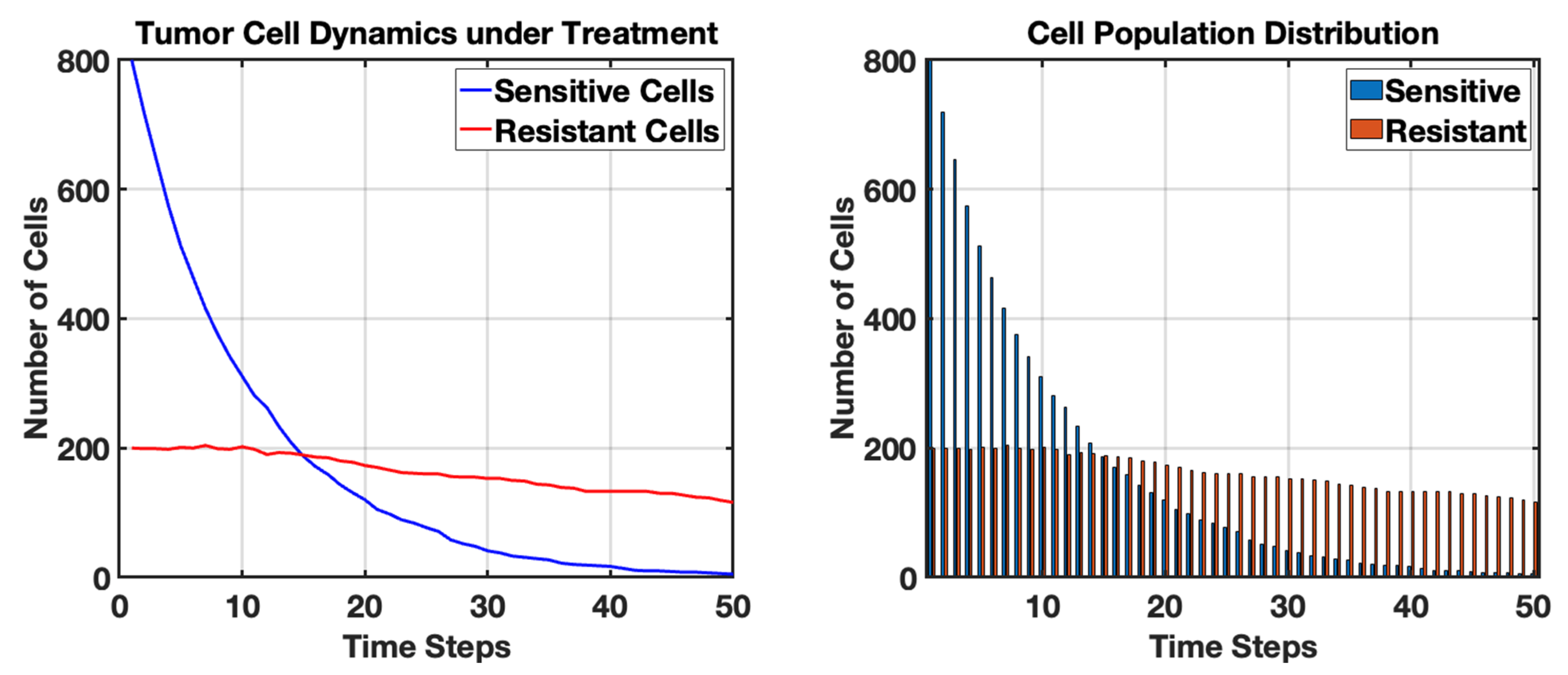
Initially, a majority of cells are sensitive to treatment, but as the treatment progresses, a notable decrease in sensitive cells is observed, reflected in the blue line on the plot. This consistent decline indicates the effectiveness of the treatment at the outset but also displays the treatment’s limitations over time.
The simulation results display the dynamic changes in populations of sensitive and resistant cancer cells over a specified treatment duration. The blue line represents the number of sensitive cells, while the red line indicates the number of resistant cells. As the simulation progresses, we observe a significant decline in the number of sensitive cells, consistent with the expectations of treatment efficacy. The inevitable emergence of resistant cells becomes evident, especially after several time steps, illustrating the challenges encountered in cancer treatment due to genetic variability and adaptation of the tumor. This trend emphasizes the risk of treatment failure as the proportion of resistant cells increases over time. Mathematically, this transition is captured through a cross-correlated noise framework, where the Wiener increments for sensitive and resistant populations are coupled by a correlation coefficient. This ensures that the stochastic fluctuations in the sensitive population’s death—representing treatment-induced selective pressure—are biologically linked to the emergence of the resistant subpopulation. This correlation reflects the bottleneck effect often observed in clinical settings, where the rapid depletion of sensitive clones provides the stochastic opportunity for rare, resistant variants to proliferate and eventually dominate the population.
These findings align with clinical observations in cancer therapies, where tumors often develop resistance to initially effective treatments. The stochastic nature of the model captures the inherent biological complexity in the tumor response, suggesting that even with continuous treatment, a subpopulation of resistant cells may survive and proliferate. This phenomenon underscores the critical need for adaptive treatment strategies and combination therapies as an approach to counteract resistance. The results serve as a foundational understanding that can aid researchers in optimizing therapeutic protocols and improving patient outcomes by highlighting the significance of monitoring tumor dynamics in response to treatment.
Next, we simulate cancer dynamics using a spatial stochastic model with different types of tumor cells, including aggressive and indolent variants (see Figure 8). In this model, we will incorporate the effects of cell migration and territoriality, demonstrating how different cell types interact over time. This simulation studies the behavior of tumor cells in a nutrient-rich environment over 100 steps. Each step represents a new cycle of growth and death for the tumor cells, taking into account the presence of nutrients that influence the speed of tumor cell growth. The visualization at each step will provide insights into how the tumor expands and interacts with healthy cells over this limited duration, helping to analyze the dynamics of cancer progression and the potential effects of nutrient availability on tumor growth.
Figure 8.
Spatial Dynamics of Indolent and Aggressive Tumor Cells After 100 Steps in a Stochastic Cancer Simulation. The grid visualizes healthy tissue (gray), indolent tumor cells (blue), aggressive tumor cells (red), and dead cells (black). The model illustrates the dynamic interactions and territorial competition between distinct tumor cell types, emphasizing the implications of growth rates and spatial distribution in understanding cancer progression and potential treatment approaches.
Figure 5, Figure 6 and Figure 8 represent a progressive refinement of the same stochastic framework. We first validated the growth-recovery balance (Figure 5), then integrated the metabolic microenvironment (Figure 6), and finally applied this unified model to simulate the territorial competition between heterogeneous phenotypes (Figure 8). While Figure 5 established the basic interaction (Healthy vs. Tumor vs. Recovery), Figure 6 added the environmental constraint (Nutrient gradients/Microenvironment), and Figure 8 adds clonal competition (Indolent vs. Aggressive variants). Figure 8 is a direct evolution of the models in Figure 5 and Figure 6, but it introduces a higher level of biological resolution by moving from a single tumor type to a multi-phenotype ecosystem.
This stochastic model investigates the spatial competition between indolent and aggressive tumor cells over a 100-step period. By limiting the simulation to 100 steps, we ensure a focused exploration of the dynamics that occur within this finite timeframe. As the simulation progresses, the indolent tumor cells, characterized by their slower growth, often find themselves outnumbered by the more aggressive cells, which invade surrounding territories more rapidly. The death probability introduces an element of instability, allowing for occasional healthy cells to reappear, although this is less frequent in the presence of aggressive growth.
The resulting landscape highlights the competitive interactions that lead to fluctuating boundaries between tumor types. Through stochastic processes such as migration and variable growth rates, the final grid visualizes the prevalence or decline of tumor types and the resultant healthy tissue. This provides valuable insights into how distinct tumor phenotypes may influence cancer treatment strategies, as therapeutic interventions could be tailored based on the proportions and behaviors of the tumor cells observed within similar models.
Additionally, we simulate spatial modeling of tumor progression using a cellular automaton approach (see Figure 9). This model will simulate the growth of a tumor in a two-dimensional grid, where each cell can represent healthy tissue, tumor cells, or dead cells. The tumor cells will proliferate based on specific rules, demonstrating spatial dynamics and interactions with their environment. This simulation consolidates the rules from previous figures to simulate the emergence of a necrotic core and the resulting non-linear growth dynamics.
Figure 9.
Spatial modeling of tumor progression in a 100 × 100 grid over 100 timesteps: (left) final configuration of the tumor, represented in red over healthy tissue (white) and dead cells (gray); (right) graph showing the tumor area (red) and the number of dead cells (black dashed line) over time, indicating the dynamics of tumor growth and necrosis within the surrounding tissue. The general upward trend in the right subplot is the numerical realization of a Stochastic Logistic Growth Equation.
The results of the spatial modeling of tumor progression illustrate the dynamic interactions between tumor cells, healthy tissue, and the processes of cell death and proliferation. The final configuration of the tumor, represented in red on the grid, shows a clearly defined area occupied by tumor cells amidst the healthy tissue (depicted in white) and dead cells (indicated in gray). This spatial distribution reflects the complex nature of tumor growth, where tumor cells successfully invade surrounding healthy tissue over time. The rules governing cell proliferation and death, driven by defined probabilities, create a realistic simulation of how tumors can expand and potentially establish a foothold in adjacent healthy regions. The presence of dead cells is indicative of the variability in tumor cell survival, which may result from factors such as nutrient competition, immune response, or therapy-induced effects.
The graph accompanying the results provides critical insights into the temporal dynamics of tumor growth and cell death. Over the simulation’s 100 timesteps, the total area occupied by tumor cells shows a general upward trend, signaling effective tumor expansion despite the presence of dead cells. This outcome highlights the resilience of tumor cells to proliferate even in the face of mortality among their ranks. The average values captured in the tumor area versus the number of dead cells reveal the intricate balance between growth and death within the tumor microenvironment. As the tumor expands, the increase in dead cells suggests that the growth may not be linear; rather, it reflects the competition for resources and environmental pressure exerted on the tumor cells. Understanding these trends is crucial for developing therapeutic strategies aimed at targeting tumor growth while considering the inherent complexities of tumor biology. The clearly defined area in Figure 9 and the non-linear growth in the accompanying graph are the analytical results of our Spatial-Stochastic framework.
To start with clinical application of stochastic modeling, we compare a Low-Dose Frequent schedule versus a High-Dose Infrequent schedule to see which one better controls the stochastic biomarker (See Figure 10).
Figure 10.
Stochastic Optimization in Drug Development. The High-Dose Pulse (Orange) shows rapid biomarker suppression followed by significant stochastic escape as the drug clears the system, potentially allowing for tumor regrowth between cycles. In contrast, the Low-Dose Frequent approach (Teal) maintains a more stable suppression closer to the therapeutic target. This modeling allows researchers to account for inter-patient variability () and metabolic clearance rates (), ensuring that the selected dose is robust against random physiological fluctuations before proceeding to human clinical trials.
Figure 10 demonstrates the use of stochastic models to optimize dosing regimens during drug development. The model evaluates how different frequencies and intensities of drug administration impact the biomarker level B, governed by the SDE.
Furthermore, we modeled the application of the stochastic differential equation in a clinical monitoring context (See Figure 11).
Figure 11.
Stochastic Biomarker Dynamics as a Real-Time Prognostic Tool. Patient A (Green) represents a positive treatment response, where the therapy effectively reduces the baseline production rate (), leading to a downward trend in biomarker expression despite inherent biological noise. Patient B (Red) demonstrates a refractory or resistant profile; the production rate remains high, indicating that the oncogenic signaling pathways are not being inhibited. The erratic fluctuations in both trajectories represent the stochastic term (), capturing random microenvironmental variations and measurement noise. Clinically, this model acts as a prognostic indicator, allowing for the early identification of non-responders by distinguishing between temporary stochastic spikes and a true therapeutic failure, thereby informing more rapid adjustments in patient management.
In Figure 11, we simulated a patient starting a new therapy. We used the stochastic modeling to calculate the probability that the treatment is actually working.
Finally, we simulated the Stochastic Dynamics of Clonal Competition and Competitive Release in Figure 12.
Figure 12.
Stochastic Modeling of Clonal Competition and Therapeutic Escape A. Pre-Treatment Phase (t < 30). B. Treatment Initiation (t = 30). C. Competitive Release and Rebound (t > 30). This simulation illustrates the evolutionary arms race within a tumor under therapeutic pressure. Initially, sensitive cells (N_s) dominate the niche due to a higher growth rate (). Upon treatment initiation at t = 30, the sensitive population is rapidly depleted by the drug’s kill rate (). This leads to competitive release: by removing the sensitive competitors, the ecological constraints of the carrying capacity (K) are lifted, allowing the resistant clones ()—previously suppressed and rare—to proliferate and dominate the tumor mass. The jagged trajectories represent the stochastic noise ( dB) of random mutations and microenvironmental fluctuations that drive unpredictable patient outcomes and the eventual emergence of treatment-refractory disease.
In the absence of selective pressure, the sensitive population () dominates the tumor microenvironment due to its superior intrinsic growth rate (). The resistant population (), which typically carries a metabolic fitness cost for maintaining defensive mechanisms (e.g., drug efflux pumps), remains at a low frequency. The stochastic fluctuations (jagged lines) represent the demographic noise ( dB) inherent in cellular proliferation and the random occurrence of point mutations () that transition cells from a sensitive to a resistant state. The introduction of a cytotoxic agent (C) significantly increases the death rate of sensitive cells (), leading to a rapid decline in the blue curve. This represents the Pharmacodynamic (PD) response where the therapeutic index is high enough to induce widespread apoptosis in the susceptible population. As is eradicated, the total biomass decreases, effectively “opening up” the carrying capacity (K). This removes the environmental constraints (nutrient scarcity and physical pressure) that were previously suppressing the resistant clones. The resistant population () undergoes competitive release, expanding exponentially to occupy the newly available niche. The final state illustrates treatment failure, where the tumor has evolved into a purely refractory mass, rendering the initial therapy ineffective.
8. Discussion
The application of stochastic modeling to cancer research underscores the fundamental reality that tumor progression is a non-linear, evolutionary process rather than a simple accumulation of mass. By formalizing parameters such as mutational influx (), phenotypic volatility (), and the fitness advantage of resistant clones (), these models provide a rigorous mathematical language to describe why treatments that appear successful in the short term often fail due to the emergence of refractory populations. The discussion of these dynamics reveals that the tumor microenvironment—characterized by shifting hypoxic fractions (H) and spatial diffusion constraints (D)—acts as a selective filter that drives clonal diversity. Consequently, the traditional clinical goal of maximum cell kill is being re-evaluated through the lens of these models, which suggest that aggressive intervention may inadvertently accelerate the competitive release of the most dangerous, resistant cells by eliminating their sensitive competitors.
Furthermore, the translational utility of these stochastic frameworks in clinical trial design and personalized medicine represents a significant leap toward engineering patient outcomes. By simulating virtual cohorts using Monte Carlo methods and updating individual prognostic trajectories through Bayesian inference, we can quantify the uncertainty horizon ( dB) that previously hindered long-term forecasting. This shift allows for the development of adaptive therapeutic protocols where drug dosing (u(t)) is dynamically adjusted in response to real-time biomarker fluctuations (, ), effectively turning the treatment process into a controlled feedback loop. As we move forward, the integration of multi-omic data into these SDE frameworks will likely reveal deeper correlations between stochastic molecular noise and clinical resistance, providing the predictive power necessary to transform cancer from an unpredictable terminal illness into a manageable chronic condition.
This study presents a transformative approach to understanding the complexities of tumor behavior and treatment dynamics. By capturing the inherent randomness in cellular processes, these models allow for a more nuanced analysis of tumor growth kinetics, evolutionary dynamics, and treatment responses. Stochastic frameworks provide insights into the variability observed in clinical outcomes, reflecting the diverse genetic landscapes and microenvironments of tumors. Furthermore, the integration of spatial modeling enhances our understanding of tumor progression, particularly regarding invasive behaviors and metastatic spread, revealing how spatial interactions within the tumor microenvironment influence treatment efficacy and disease outcomes. The richness of these models facilitates the exploration of various therapeutic scenarios, offering more accurate predictions that can support personalized treatment plans and dynamic clinical decision-making.
In addition to the insights gained from tumor growth kinetics and treatment responses, stochastic modeling can elucidate the role of cellular heterogeneity in cancer. The acknowledgment that tumors consist of a diverse array of cell types, each with distinct genetic and phenotypic characteristics, is critical for understanding treatment resistance and relapse. Stochastic models can simulate the interactions among these subpopulations and their adaptive responses to therapies, thereby revealing the evolutionary pressures that lead to the selection of resistant cells. This dynamic perspective encourages a shift from traditional one-size-fits-all treatment strategies to more nuanced approaches that consider the specific subclonal architectures of individual tumors.
Moreover, the integration of patient-derived data into stochastic modeling frameworks can significantly enhance their predictive capabilities. Utilizing real-world patient data, such as genomics, transcriptomics, and clinical outcomes, allows researchers to calibrate stochastic models more effectively, ensuring that they accurately reflect the complexities of human cancer. Such model-driven approaches can support more robust simulations of treatment scenarios, helping clinicians to anticipate potential resistance pathways and adapt therapy plans accordingly. As the field of personalized medicine continues to evolve, the ability to leverage stochastic modeling alongside patient-specific data will be essential in refining treatment strategies and improving patient management.
Another important dimension of stochastic modeling is the potential to assess the impact of combinatorial therapies on treatment outcomes. Cancer treatment often involves the use of multiple agents targeting different pathways simultaneously. Stochastic models can be employed to explore the synergies and antagonisms that arise when combining therapies, providing insights into optimal treatment regimens. By analyzing various drug combinations through stochastic simulations, researchers can predict which combinations may increase the likelihood of overcoming resistance or achieving better patient responses. Such models can guide clinical trial designs by identifying candidate treatment pairs that warrant further investigation in clinical settings, ultimately accelerating the development of more effective therapeutic strategies.
The integration of real-time monitoring technologies, such as liquid biopsies and imaging techniques, with stochastic modeling represents an exciting frontier in cancer research. By continuously updating models with real-time data on tumor evolution and treatment response, clinicians could glean actionable insights and adapt treatments in a responsive manner. Such adaptive clinical approaches, supported by robust stochastic modeling frameworks, could transform cancer care into a highly personalized and dynamic process. The capability to adjust therapies based on the evolving characteristics of a tumor would not only enhance treatment outcomes but also empower patients by involving them in their treatment journey. As research and technology continue to advance, the synergy between stochastic modeling and real-time patient data could play a pivotal role in redefining cancer treatment paradigms.
8.1. Significance of This Work
This work is significant as it highlights the critical role of stochastic modeling in advancing our understanding of cancer biology and treatment strategies. The novelty of this study lies in its departure from traditional deterministic frameworks to a multi-scale, adaptive approach that treats cancer as a dynamic, probabilistic ecosystem rather than a linear growth process. By embracing the inherent uncertainties of tumor behavior through the use of Stochastic Differential Equations (SDEs), this research introduces a robust methodology for quantifying the ‘evolutionary velocity’ of a tumor in real-time. By moving beyond a single-scale approach and incorporating the stochastic resonance between nutrient diffusion (PDEs) and cellular population shifts (SDEs), this paper provides a new analytical tool for quantifying Evolutionary Risk. This allows researchers to predict treatment escape as a function of environmental volatility rather than just static tumor size, representing a significant shift from descriptive modeling to predictive, biologically anchored clinical simulation.
Unlike previous models that prioritize population averages, this work provides a framework for in silico therapeutic testing, allowing for the simulation of patient-specific ‘what-if’ scenarios based on individual biomarker noise () and clearance kinetics (). These insights have the potential to reshape clinical practices by moving beyond static protocols toward strategies tailored to the unique genetic and environmental contexts of individual tumors. As a result, the integration of stochastic modeling into cancer research could significantly enhance our capability to develop effective therapies, ultimately improving patient outcomes and contributing to the ongoing fight against cancer.
8.2. Limitations
Despite the strengths of stochastic modeling, several limitations must be acknowledged (see Table 18). One major challenge is the reliance on accurate input parameters and biological assumptions; incorrect assumptions or data can lead to misleading conclusions. Additionally, models often require simplifications that may not capture the full complexity of tumor biology, such as the influence of the immune system or the multifaceted nature of tumor–stroma interactions. The computational intensity of stochastic simulations can also pose limitations, particularly for large-scale applications or when integrating high-dimensional data. Finally, the translation of these models into clinical practice remains a significant hurdle, as there is often a gap between theoretical modeling and practical implementation in diverse patient populations. Furthermore, a critical limitation lies in the calibration of models against real-world patient and experimental data. Clinical data are often sparse, irregularly sampled, and subject to significant measurement error, which makes it difficult to distinguish true biological stochasticity ( dB) from observation noise. Experimental data derived from in vitro or in vivo models frequently fail to reflect the patient-to-patient variability seen in the clinic, leading to overfitting where a model perfectly describes a specific dataset but fails to predict outcomes for a broader, more heterogeneous patient population. This disconnect between high-resolution mathematical theory and low-resolution clinical data often restricts the model’s ability to provide high-confidence, individualized prognostications.
Table 18.
Limitations in stochastic modeling, including biological and technical factors, and their impact on model accuracy and interpretability.
8.3. Future Work
Future research should focus on refining stochastic models by incorporating multi-scale approaches that combine molecular, cellular, and tissue-level data. Enhancing the integration of genomic and transcriptomic information within stochastic frameworks could improve model accuracy and predictive capacity. Collaboration with experimentalists to validate predictions against empirical data will also be crucial in advancing model robustness. Moreover, the development of user-friendly computational tools and platforms that facilitate the application of these models in clinical settings is essential. Finally, exploring the potential of machine learning techniques to augment traditional stochastic modeling could lead to new insights and improve the model’s adaptability to evolving tumor landscapes.
9. Conclusions
In conclusion, this work underscores the transformative potential of stochastic modeling in cancer research and clinical practice. By capturing the inherent variability and complexity of tumor behavior, these models provide invaluable insights into tumor dynamics, treatment responses, and cellular heterogeneity. The ability to simulate diverse scenarios allows researchers and clinicians to explore personalized treatment strategies that are better aligned with the unique characteristics of individual patients’ tumors. Moreover, the integration of patient-derived data and advancements in real-time monitoring technologies enhances the applicability of stochastic models in clinical settings, making them powerful tools for guiding therapeutic decisions. While there are challenges and limitations to overcome, including model validation and computational constraints, the future trajectory of stochastic modeling holds significant promise. As we move towards a more tailored approach in oncology, the incorporation of stochastic methodologies will be crucial for deciphering the complexities of cancer. This research not only provides a foundation for further exploration in the field, but it also emphasizes the need for interdisciplinary collaboration among modelers, biologists, and clinicians to realize the full potential of these approaches. Ultimately, harnessing the power of stochastic modeling may lead to improved therapeutic outcomes, providing hope for patients facing the challenges of cancer. Through innovation, validation, and real-world application, this work lays the groundwork for a future in which personalized cancer care is driven by deeper understanding and predictive insights into the behavior of tumors.
To conclude, the shift toward stochastic modeling in oncology represents a transition from reactive medicine to proactive, evolutionary management. By synthesizing variables across multiple scales—from the microscopic mutation rate () and molecular biomarker synthesis () to the macroscopic carrying capacity (K) and therapeutic efficacy ()—these frameworks provide a unified map of the arms race between clinical intervention and tumor adaptation. The ultimate value of these models lies in their ability to quantify the known unknowns represented by stochastic volatility (), allowing clinicians to design trials and treatment protocols that are robust against the inherent randomness of biology. As these mathematical tools continue to be refined by real-time patient data, they promise a future where the unpredictability of cancer is replaced by a calculated, adaptive strategy that prioritizes long-term survival and the preservation of patient quality of life.
Funding
This research received no external funding.
Data Availability Statement
No new data were created or analyzed in this study.
Conflicts of Interest
The author declares no conflicts of interest.
References
- Feng, J.; Zhang, X.; Tian, T. Mathematical Modeling and Inference of Epidermal Growth Factor-Induced Mitogen-Activated Protein Kinase Cell Signaling Pathways. Int. J. Mol. Sci. 2024, 25, 10204. [Google Scholar] [CrossRef] [Scilit]
- Olushola, A.; Alao, V. Biomathematics in Cancer Research: Looking into How Mathematical Models Are Used to Understand Tumor Growth and the Effectiveness of Different Treatment Strategies. Preprint 2024. [Google Scholar] [CrossRef] [Scilit]
- Hassan, J.; Saeed, S.M.; Deka, L.; Uddin, M.J.; Das, D.B. Applications of Machine Learning (ML) and Mathematical Modeling (MM) in Healthcare with Special Focus on Cancer Prognosis and Anticancer Therapy: Current Status and Challenges. Pharmaceutics 2024, 16, 260. [Google Scholar] [CrossRef] [Scilit]
- Benson, T.O. Mathematical and Computational Modelling of Immune Cell Responses in Cell Migration. In Cell Migration in Development, Health and Disease; Springer Nature: Cham, Switzerland, 2024; pp. 315–336. [Google Scholar]
- Casotti, M.C.; Meira, D.D.; Zetum, A.S.S.; Campanharo, C.V.; da Silva, D.R.C.; Giacinti, G.M.; da Silva, I.M.; Moura, J.A.D.; Barbosa, K.R.M.; Altoé, L.S.C.; et al. Integrating frontiers: A holistic, quantum and evolutionary approach to conquering cancer through systems biology and multidisciplinary synergy. Front. Oncol. 2024, 14, 1419599. [Google Scholar] [CrossRef] [Scilit]
- Kulesza, A.; Couty, C.; Lemarre, P.; Thalhauser, C.J.; Cao, Y. Advancing cancer drug development with mechanistic mathematical modeling: Bridging the gap between theory and practice. J. Pharmacokinet. Pharmacodyn. 2024, 51, 581–604. [Google Scholar] [CrossRef] [Scilit] [PubMed]
- Yazdanpanah, N.; Dochy, F.; Darmstadt, G.L.; Peters, G.J.; Tsitlakidis, A.; Aifantis, E.C.; Cerda, A.; Comini, E.; Brand, S.; Gupta, M.; et al. Cancer: A Complex Problem Requiring Interdisciplinary Research. In Cancer Treatment: An Interdisciplinary Approach; Springer Nature: Cham, Switzerland, 2023; pp. 1–45. [Google Scholar]
- Azizi, T. Intersections of Neurobiology and Oncology: Foundations and Frontiers in Cancer Neuroscience; Sciencedomain International: Delhi, India, 2024. [Google Scholar]
- Janes, K.A.; Lazzara, M.J. Systems Biology of the Cancer Cell. Annu. Rev. Biomed. Eng. 2014, 27, 1–28. [Google Scholar] [CrossRef] [Scilit] [PubMed]
- Rockne, R.C.; Hawkins-Daarud, A.; Swanson, K.R.; Sluka, J.P.; Glazier, J.A.; Macklin, P.; Hormuth, D.A.; Jarrett, A.M.; Lima, E.A.B.F.; Oden, J.T.; et al. The 2019 mathematical oncology roadmap. Phys. Biol. 2019, 16, 041005. [Google Scholar] [CrossRef] [Scilit]
- Azizi, T. Mathematical Modeling of Cancer Progression. AppliedMath 2024, 4, 1065–1079. [Google Scholar] [CrossRef] [Scilit]
- Azizi, T. Mathematical Modelling of Cancer Treatments, Resistance, Optimization. AppliedMath 2025, 5, 40. [Google Scholar] [CrossRef] [Scilit]
- Azizi, T. Mathematical Modeling with Applications in Biological Systems, Physiology, and Neuroscience. Ph.D. Thesis, Kansas State University, Manhattan, KS, USA, 2021. [Google Scholar]
- Mukherjee, A.; Abraham, S.; Singh, A.; Balaji, S.; Mukunthan, K.S. From Data to Cure: A Comprehensive Exploration of Multi-omics Data Analysis for Targeted Therapies. Mol. Biotechnol. 2024, 67, 1269–1289. [Google Scholar] [CrossRef] [Scilit]
- Al-Ghazawi, M.; Salameh, H.; Amo-Afful, S.; Khasawneh, S.; Ghanem, R. An In-Depth Look Into the epidemiological and etiological aspects of prostate cancer: A literature review. Cureus 2023, 15, e48252. [Google Scholar] [CrossRef] [Scilit] [PubMed]
- Ashfaq, U.A. Role of Computational Biology. In Human Microbiome: Techniques, Strategies, and Therapeutic Potential; Springer: Berlin/Heidelberg, Germany, 2024; pp. 85–117. [Google Scholar]
- Dagogo-Jack, I.; Shaw, A.T. Tumour heterogeneity and resistance to cancer therapies. Nat. Rev. Clin. Oncol. 2018, 15, 81–94. [Google Scholar] [CrossRef] [Scilit]
- Ottaiano, A.; Ianniello, M.; Santorsola, M.; Ruggiero, R.; Sirica, R.; Sabbatino, F.; Perri, F.; Cascella, M.; Di Marzo, M.; Berretta, M.; et al. From chaos to opportunity: Decoding cancer heterogeneity for enhanced treatment strategies. Biology 2023, 12, 1183. [Google Scholar] [CrossRef] [Scilit]
- Wu, F.; Fan, J.; He, Y.; Xiong, A.; Yu, J.; Li, Y.; Zhang, Y.; Zhao, W.; Zhou, F.; Li, W.; et al. Single-cell profiling of tumor heterogeneity and the microenvironment in advanced non-small cell lung cancer. Nat. Commun. 2021, 12, 2540. [Google Scholar] [CrossRef] [Scilit]
- Bhat, G.R.; Sethi, I.; Sadida, H.Q.; Rah, B.; Mir, R.; Algehainy, N.; Albalawi, I.A.; Masoodi, T.; Subbaraj, G.K.; Jamal, F.; et al. Cancer cell plasticity: From cellular, molecular, and genetic mechanisms to tumor heterogeneity and drug resistance. Cancer Metastasis Rev. 2024, 43, 197–228. [Google Scholar] [CrossRef] [Scilit]
- Ma, C.; Gurkan-Cavusoglu, E. A comprehensive review of computational cell cycle models in guiding cancer treatment strategies. NPJ Syst. Biol. Appl. 2024, 10, 71. [Google Scholar] [CrossRef] [Scilit]
- Kimmel, M. Stochasticity and determinism in models of hematopoiesis. In A Systems Biology Approach to Blood; Springer: Berlin/Heidelberg, Germany, 2024; pp. 119–152. [Google Scholar]
- Jarrett, A.M.; Lima, E.A.; Hormuth, D.A.; McKenna, M.T.; Feng, X.; Ekrut, D.A.; Resende, A.C.M.; Brock, A.; Yankeelov, T.E. Mathematical models of tumor cell proliferation: A review of the literature. Expert Rev. Anticancer Ther. 2018, 18, 1271–1286. [Google Scholar] [CrossRef] [Scilit]
- Altrock, P.M.; Liu, L.L.; Michor, F. The mathematics of cancer: Integrating quantitative models. Nat. Rev. Cancer 2015, 15, 730–745. [Google Scholar] [CrossRef] [Scilit] [PubMed]
- Kuznetsov, M.; Kolobov, A. Investigation of solid tumor progression with account of proliferation/migration dichotomy via Darwinian mathematical model. J. Math. Biol. 2020, 80, 601–626. [Google Scholar] [CrossRef] [Scilit]
- Liu, Y. Challenges in Modelling and Control of Biological Systems. Doctoral Dissertation, University of Oxford, Oxford, UK, 2024. [Google Scholar]
- Bravo, R.R. 3D Organ-Scale Models of Tumor Growth and Treatment. Doctoral Dissertation, University of South Florida, Tampa, FL, USA, 2024. [Google Scholar]
- Strauss, B.; Bertolaso, M.; Ernberg, I.; Bissell, M.J. (Eds.) Rethinking Cancer: A New Paradigm for the Postgenomics Era; MIT Press: Cambridge, MA, USA, 2021. [Google Scholar]
- Gatenby, R.A.; Brown, J.S. Integrating evolutionary dynamics into cancer therapy. Nat. Rev. Clin. Oncol. 2020, 17, 675–686. [Google Scholar] [CrossRef] [Scilit]
- Du, W.; Elemento, O. Cancer systems biology: Embracing complexity to develop better anticancer therapeutic strategies. Oncogene 2015, 34, 3215–3225. [Google Scholar] [CrossRef] [Scilit]
- Craig, M.; Jenner, A.L.; Namgung, B.; Lee, L.P.; Goldman, A. Engineering in medicine to address the challenge of cancer drug resistance: From micro-and nanotechnologies to computational and mathematical modeling. Chem. Rev. 2020, 121, 3352–3389. [Google Scholar] [CrossRef] [Scilit]
- Foo, J.; Michor, F. Evolution of acquired resistance to anti-cancer therapy. J. Theor. Biol. 2014, 355, 10–20. [Google Scholar] [CrossRef] [Scilit] [PubMed]
- Chiari, G. Epigenetic and Geometrical Characterisation of Cancer Cell Populations: A Personalised-Medicine Oriented Mathematical Study of Tumour Evolutionary Dynamics and Therapies. PhD Thesis, Università di Torino, Torino, Italy, 2024. [Google Scholar]
- Grossman, Z. Immunological paradigms, mechanisms, and models: Conceptual understanding is a prerequisite to effective modeling. Front. Immunol. 2019, 10, 2522. [Google Scholar] [CrossRef] [Scilit] [PubMed]
- Araujo, R.P.; McElwain, D.S. A history of the study of solid tumour growth: The contribution of mathematical modelling. Bull. Math. Biol. 2004, 66, 1039–1091. [Google Scholar] [CrossRef] [Scilit]
- Szymańska, Z.; Cytowski, M.; Mitchell, E.; Macnamara, C.K.; Chaplain, M.A. Computational modelling of cancer development and growth: Modelling at multiple scales and multiscale modelling. Bull. Math. Biol. 2018, 80, 1366–1403. [Google Scholar] [CrossRef] [Scilit] [PubMed]
- Irurzun-Arana, I.; Rackauckas, C.; McDonald, T.O.; Trocóniz, I.F. Beyond deterministic models in drug discovery and development. Trends Pharmacol. Sci. 2020, 41, 882–895. [Google Scholar] [CrossRef] [Scilit]
- Vernerey, F.J.; Lalitha Sridhar, S.; Muralidharan, A.; Bryant, S.J. Mechanics of 3D cell–hydrogel interactions: Experiments, models, and mechanisms. Chem. Rev. 2021, 121, 11085–11148. [Google Scholar] [CrossRef] [Scilit]
- Abuwatfa, W.H.; Pitt, W.G.; Husseini, G.A. Scaffold-based 3D cell culture models in cancer research. J. Biomed. Sci. 2024, 31, 7. [Google Scholar] [CrossRef] [Scilit]
- Aydin, O.; Passaro, A.P.; Raman, R.; Spellicy, S.E.; Weinberg, R.P.; Kamm, R.D.; Sample, M.; Truskey, G.A.; Zartman, J.; Dar, R.D.; et al. Principles for the design of multicellular engineered living systems. APL Bioeng. 2022, 6, 010903. [Google Scholar] [CrossRef] [Scilit]
- Heesterbeek, H.; Anderson, R.M.; Andreasen, V.; Bansal, S.; De Angelis, D.; Dye, C.; Eames, K.T.D.; Edmunds, W.J.; Frost, S.D.W.; Isaac Newton Institute IDD Collaboration; et al. Modeling infectious disease dynamics in the complex landscape of global health. Science 2015, 347, aaa4339. [Google Scholar] [CrossRef] [Scilit]
- Gallasch, R.; Efremova, M.; Charoentong, P.; Hackl, H.; Trajanoski, Z. Mathematical models for translational and clinical oncology. J. Clin. Bioinform. 2013, 3, 23. [Google Scholar] [CrossRef] [Scilit]
- Alfonso, S.; Jenner, A.L.; Craig, M. Translational approaches to treating dynamical diseases through in silico clinical trials. Chaos Interdiscip. J. Nonlinear Sci. 2020, 13, 123128. [Google Scholar] [CrossRef] [Scilit]
- Ramaswamy, V.D.; Keidar, M. Personalized Plasma Medicine for Cancer: Transforming Treatment Strategies with Mathematical Modeling and Machine Learning Approaches. Appl. Sci. 2023, 14, 355. [Google Scholar] [CrossRef] [Scilit]
- Saraf, S.; De, A.; Tripathy, B.K. Effective Use of Computational Biology and Artificial Intelligence in the Domain of Medical Oncology. In Computational Intelligence for Oncology and Neurological Disorders; CRC Press: Boca Raton, FL, USA, 2024; pp. 228–252. [Google Scholar]
- Metzcar, J.; Jutzeler, C.R.; Macklin, P.; Köhn-Luque, A.; Brüningk, S.C. A review of mechanistic learning in mathematical oncology. Front. Immunol. 2024, 15, 1363144. [Google Scholar] [CrossRef] [Scilit] [PubMed]
- Bizzarri, M.; Fedeli, V.; Monti, N.; Cucina, A.; Jalouli, M.; Alwasel, S.H.; Harrath, A.H. Personalization of medical treatments in oncology: Time for rethinking the disease concept to improve individual outcomes. EPMA J. 2021, 12, 545–558. [Google Scholar] [CrossRef] [Scilit] [PubMed]
- Hastings, J.F.; O’Donnell, Y.E.; Fey, D.; Croucher, D.R. Applications of personalised signalling network models in precision oncology. Pharmacol. Ther. 2020, 212, 107555. [Google Scholar] [CrossRef] [Scilit]
- Gerlee, P. The model muddle: In search of tumor growth laws. Cancer Res. 2013, 73, 2407–2411. [Google Scholar] [CrossRef] [Scilit]
- Sarapata, E.A.; De Pillis, L.G. A comparison and catalog of intrinsic tumor growth models. Bull. Math. Biol. 2014, 76, 2010–2024. [Google Scholar] [CrossRef] [Scilit]
- Chmielecki, J.; Foo, J.; Oxnard, G.R.; Hutchinson, K.; Ohashi, K.; Somwar, R.; Wang, L.; Amato, K.R.; Arcila, M.; Sos, M.L.; et al. Optimization of dosing for EGFR-mutant non–small cell lung cancer with evolutionary cancer modeling. Sci. Transl. Med. 2011, 3, 90ra59. [Google Scholar] [CrossRef] [Scilit]
- Haeno, H.; Gonen, M.; Davis, M.B.; Herman, J.M.; Iacobuzio-Donahue, C.A.; Michor, F. Computational modeling of pancreatic cancer reveals kinetics of metastasis suggesting optimum treatment strategies. Cell 2012, 148, 362–375. [Google Scholar] [CrossRef] [Scilit] [PubMed]
- Tannock, I.F. The relation between cell proliferation and the vascular system in a transplanted mouse mammary tumour. Br. J. Cancer 1968, 22, 258. [Google Scholar] [CrossRef] [Scilit] [PubMed]
- Gatenby, R.A.; Gillies, R.J. Why do cancers have high aerobic glycolysis? Nat. Rev. Cancer 2004, 4, 891–899. [Google Scholar] [CrossRef] [Scilit] [PubMed]
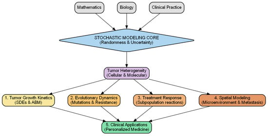
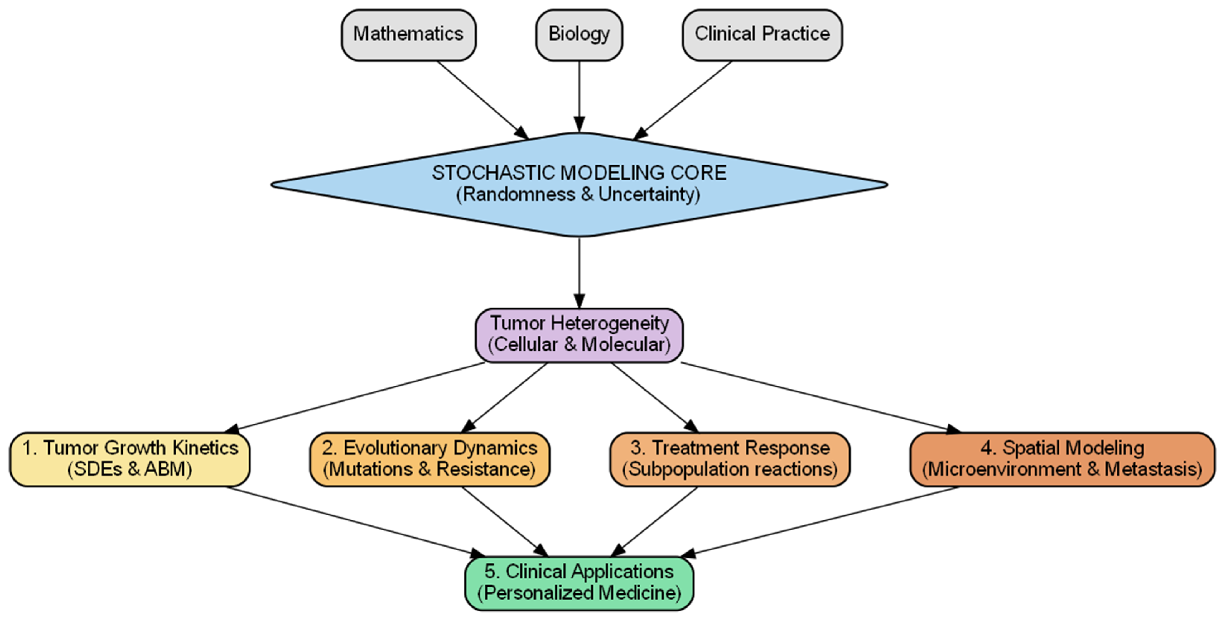
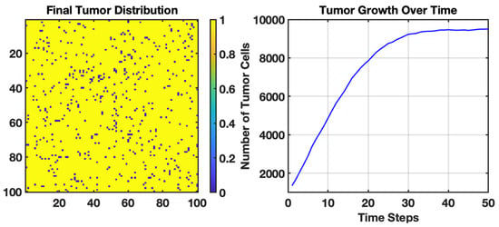
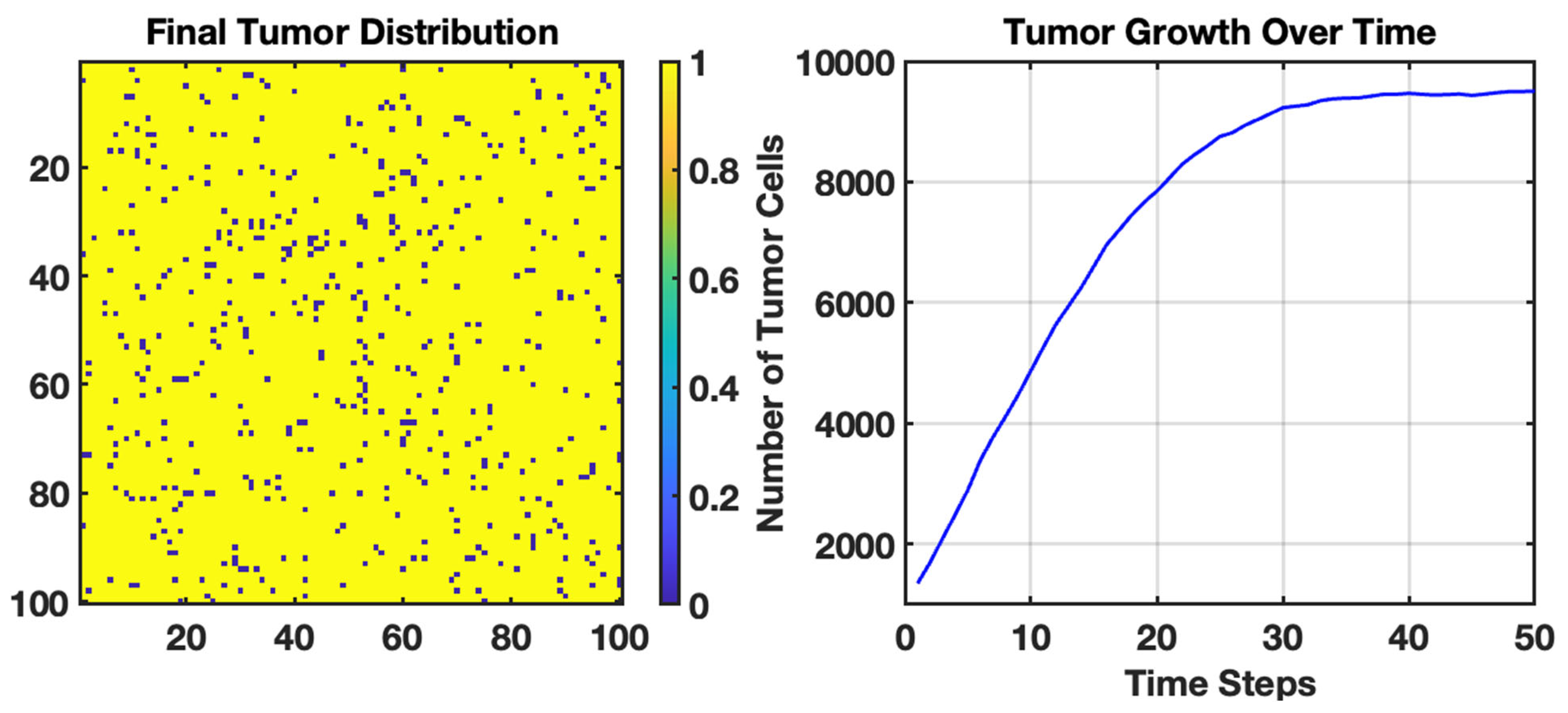
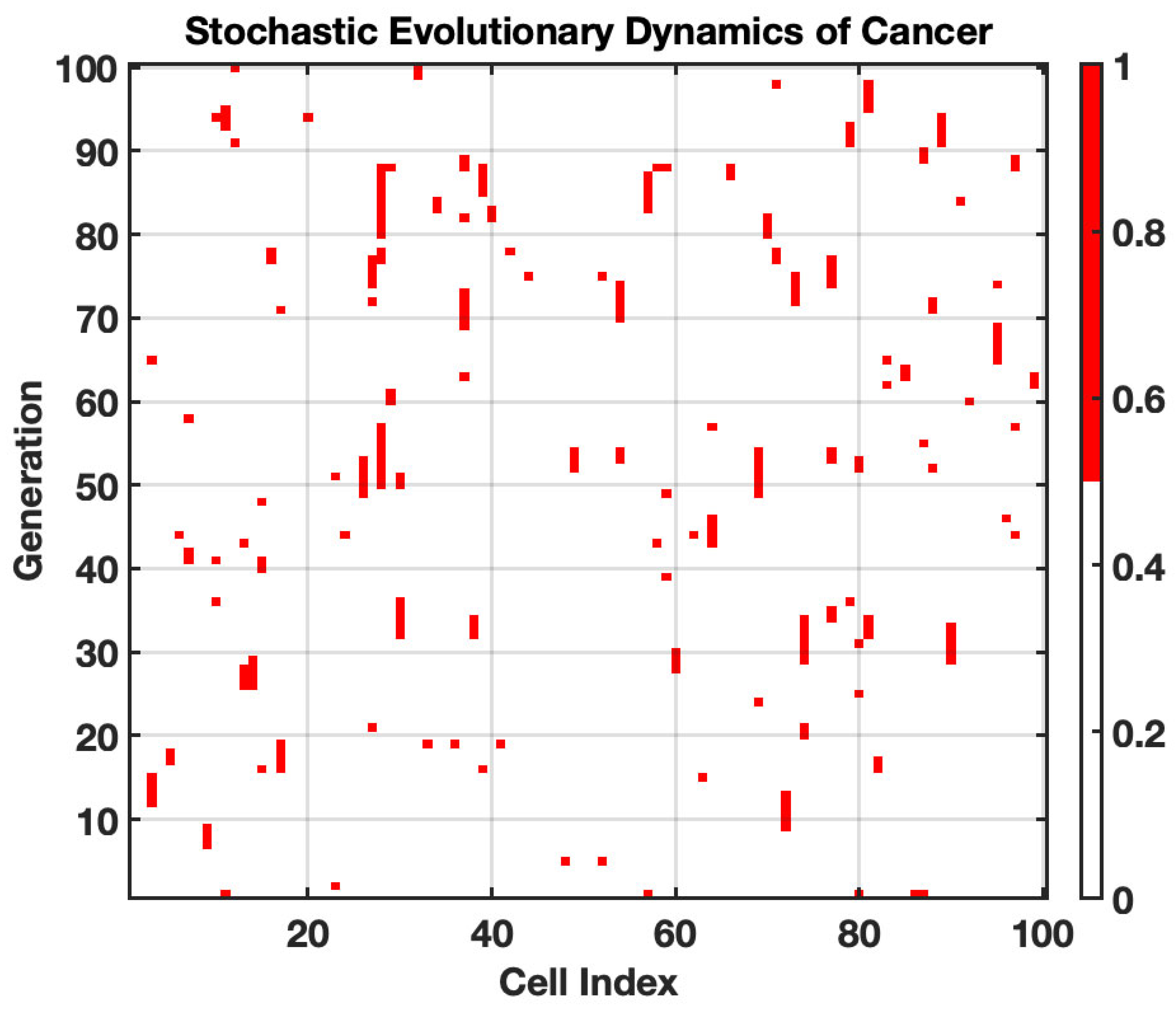
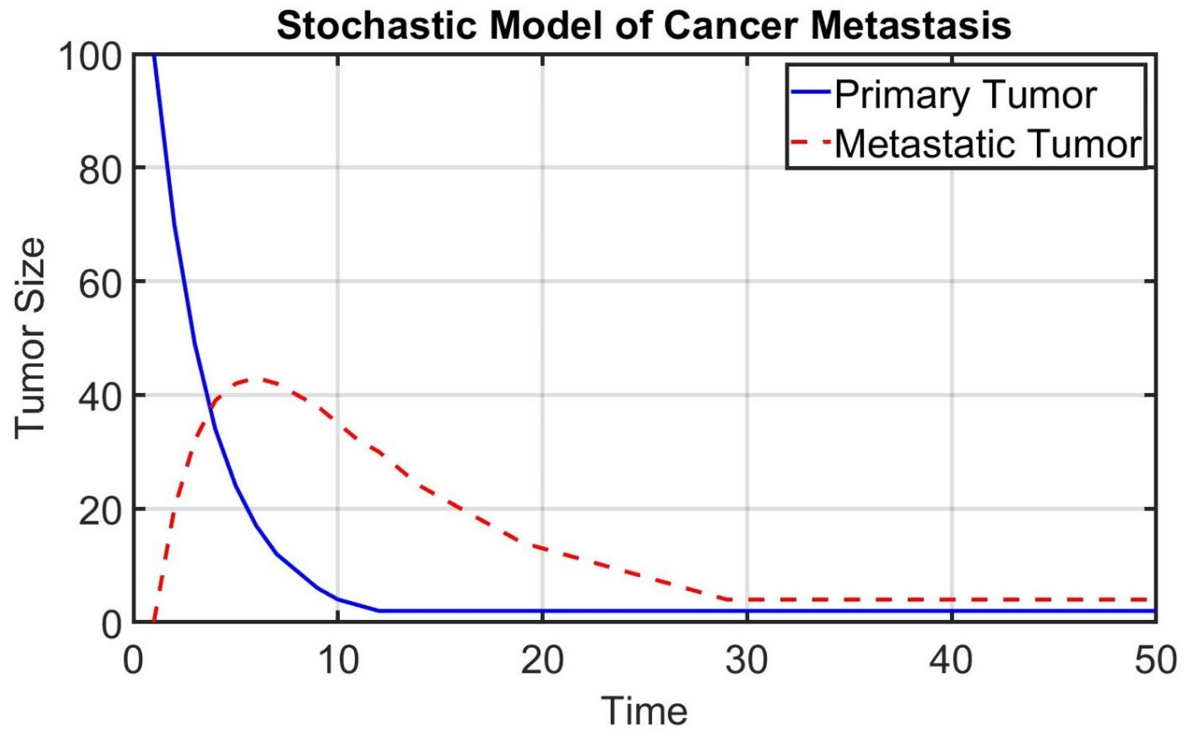
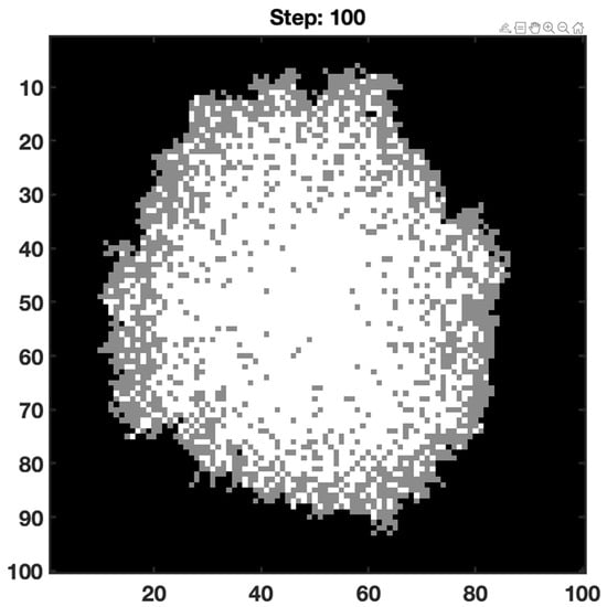
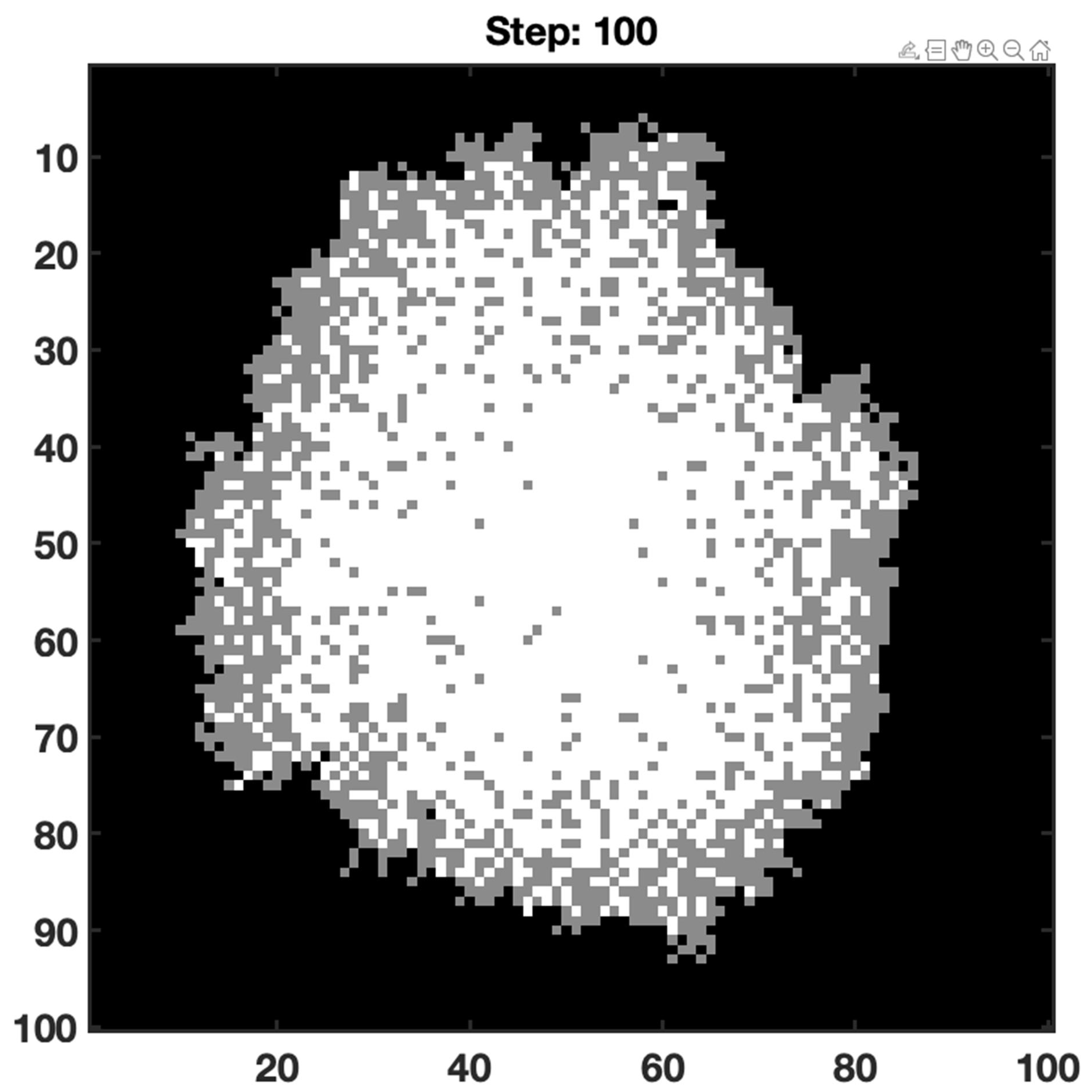
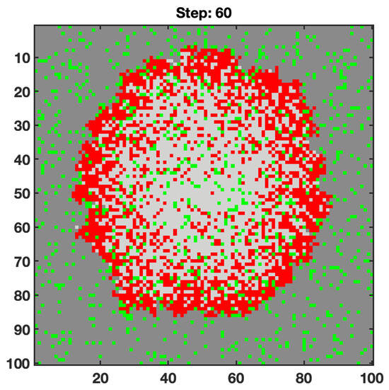
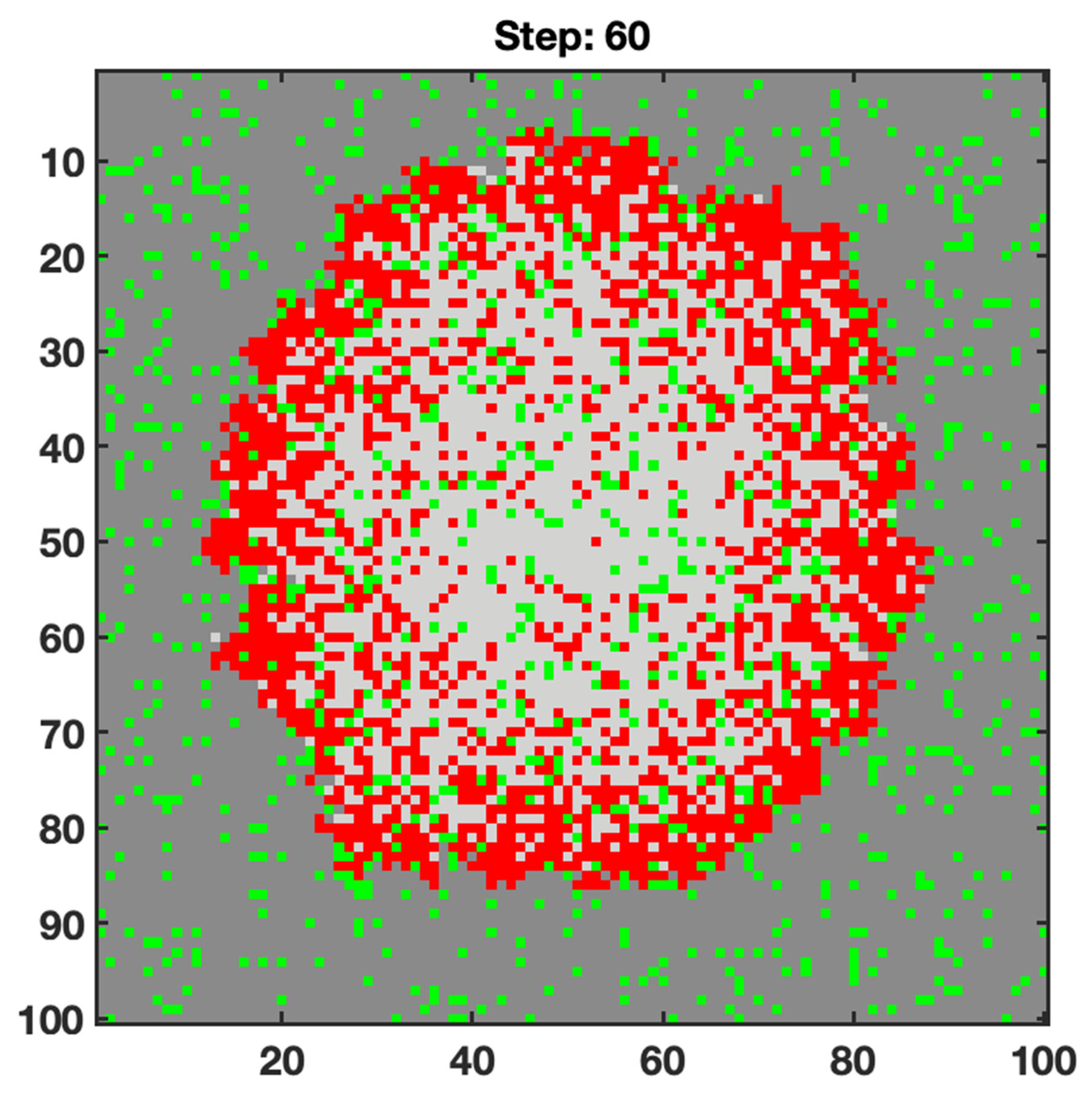
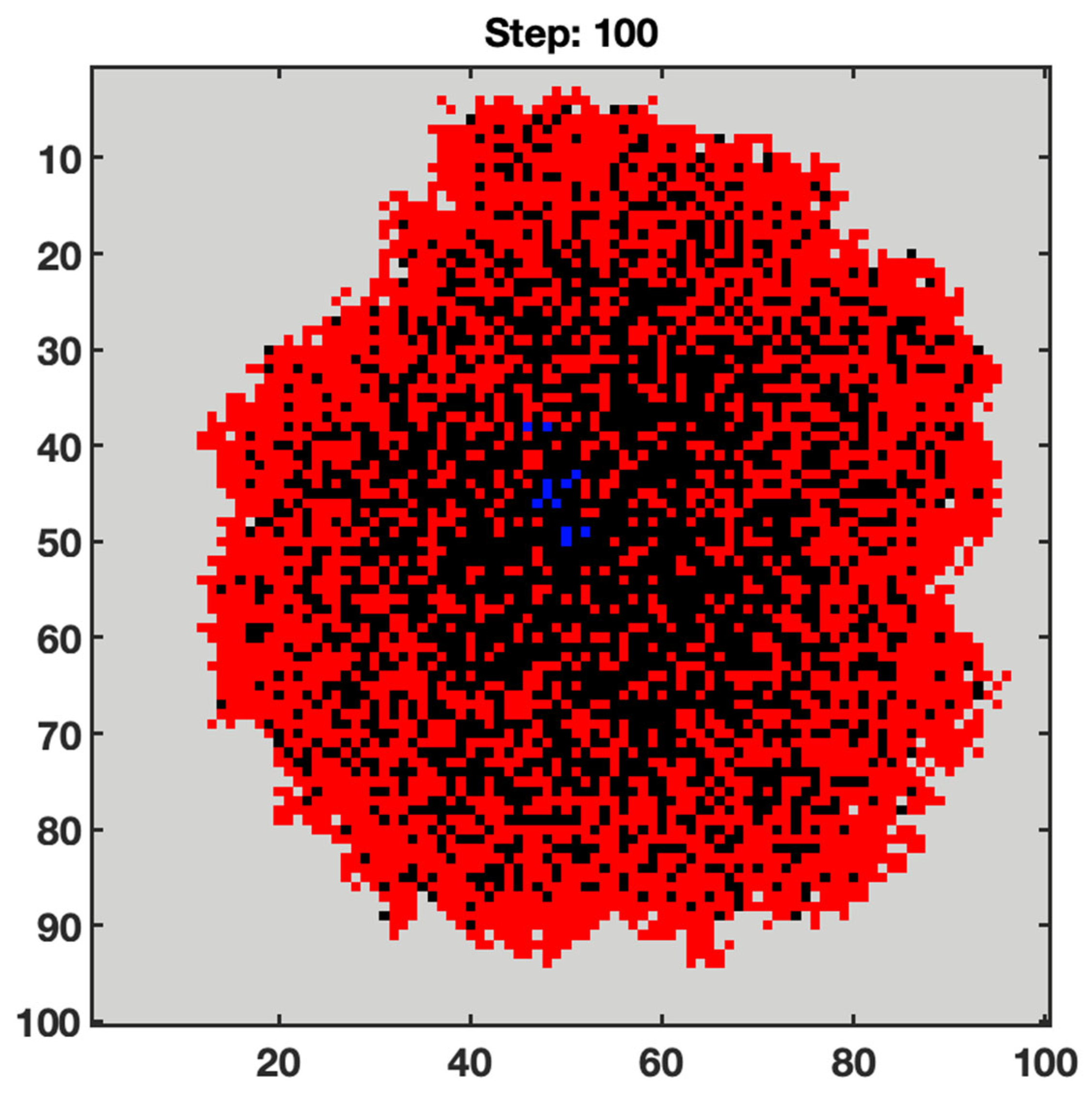
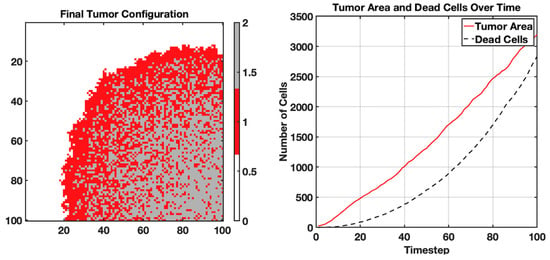
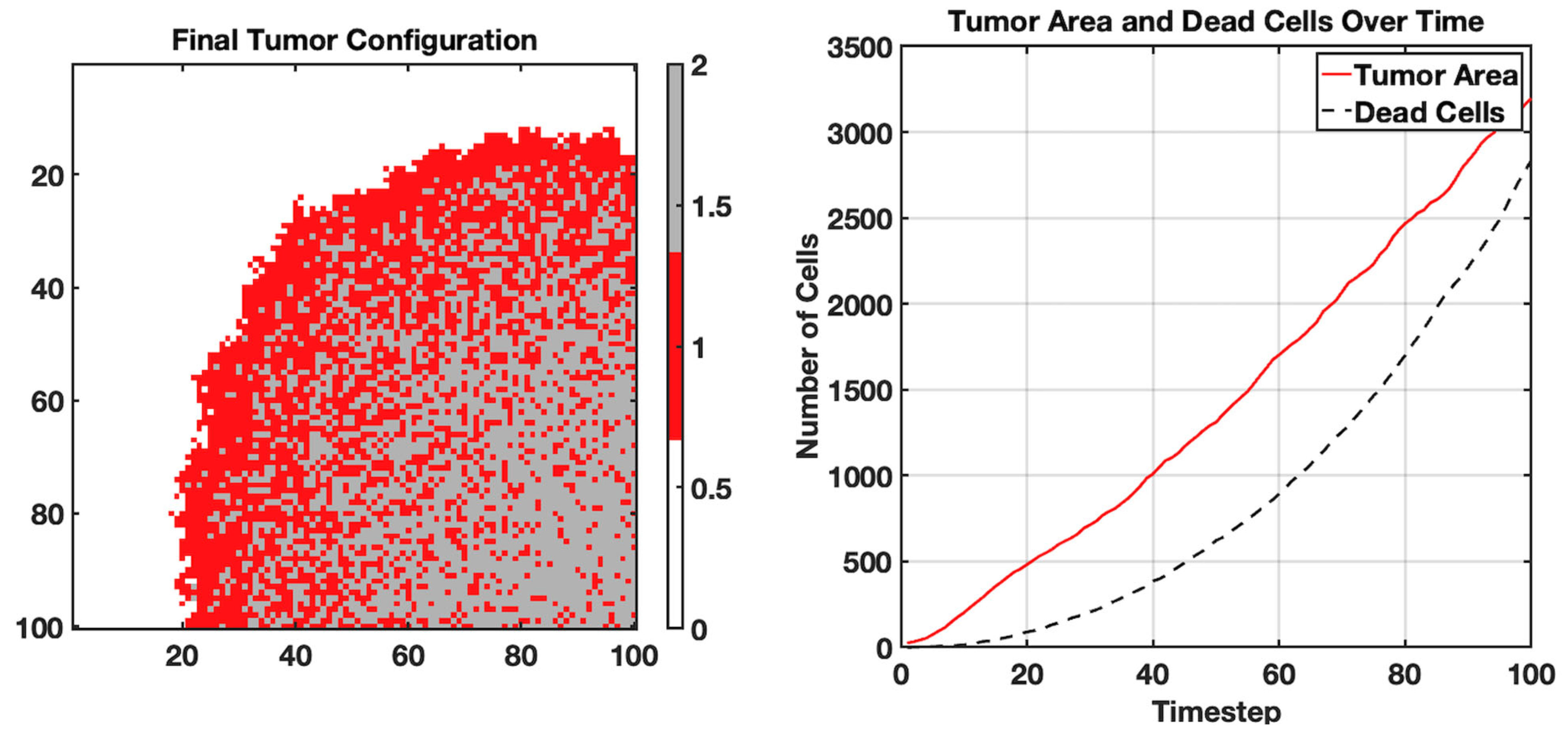
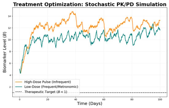
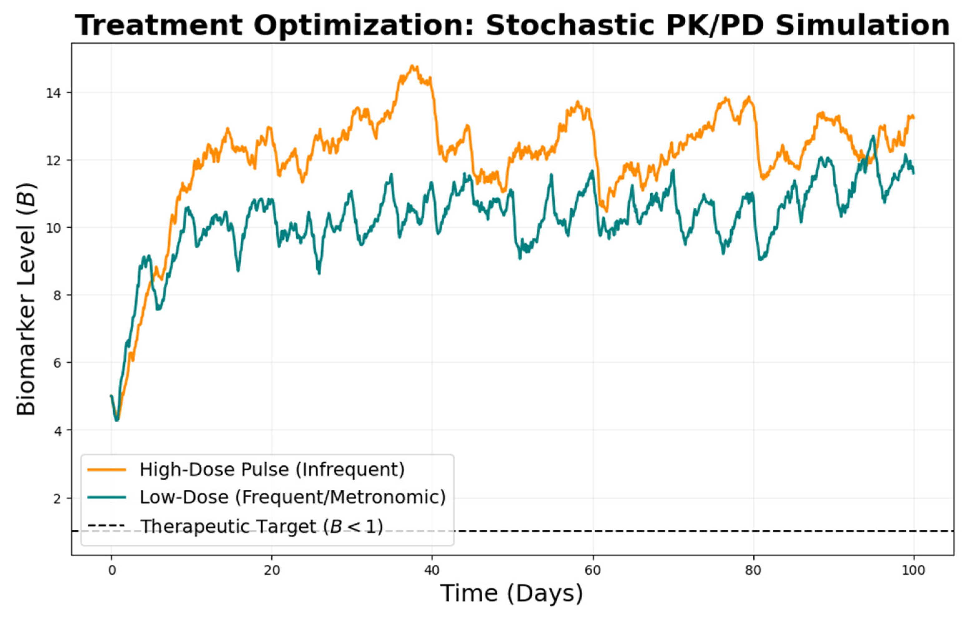
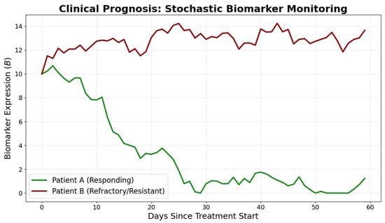
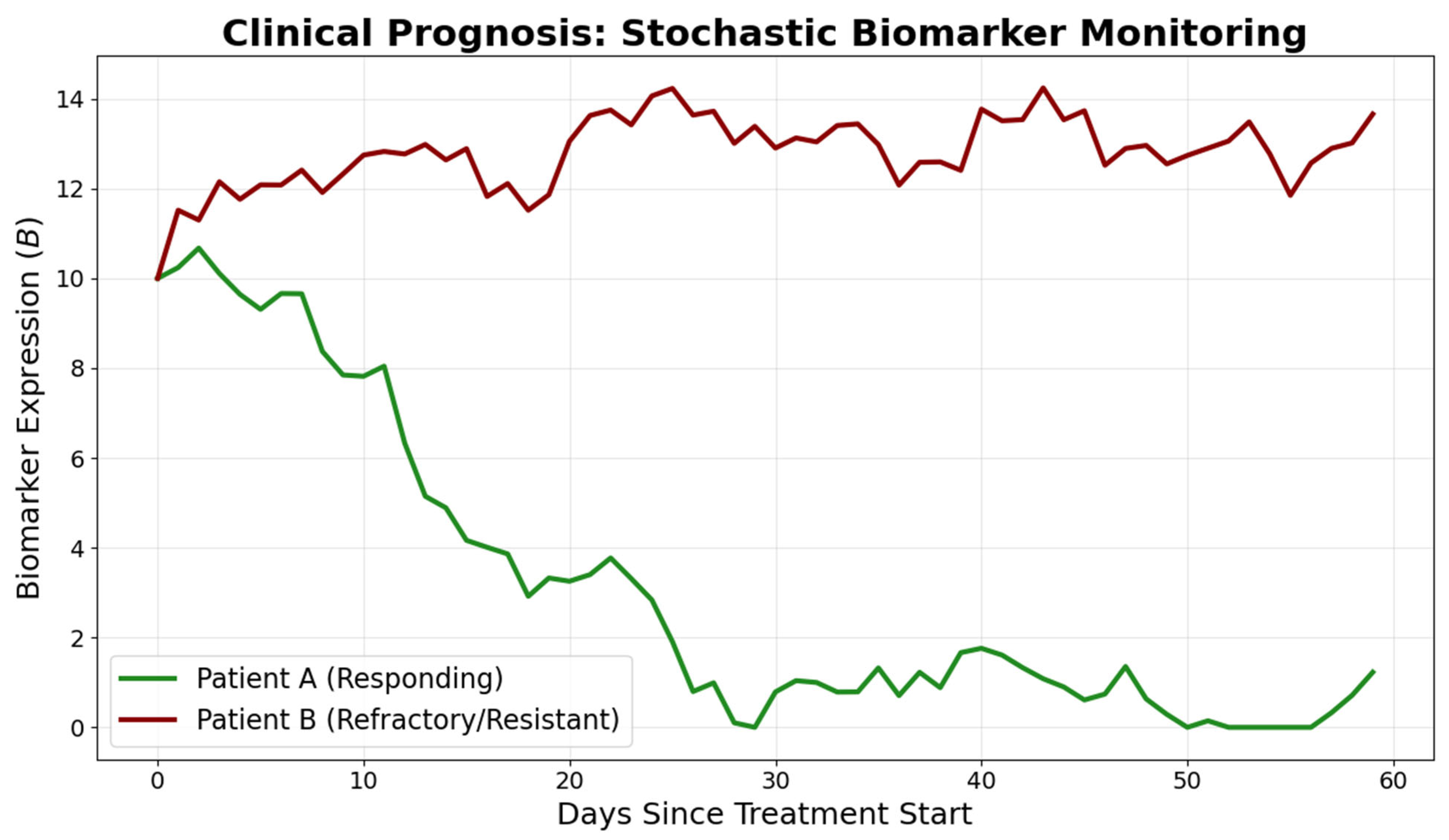
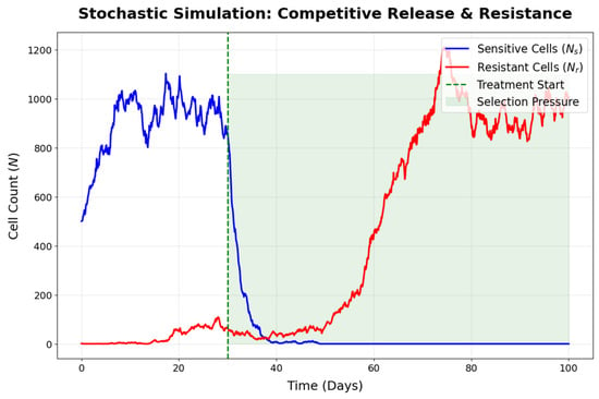
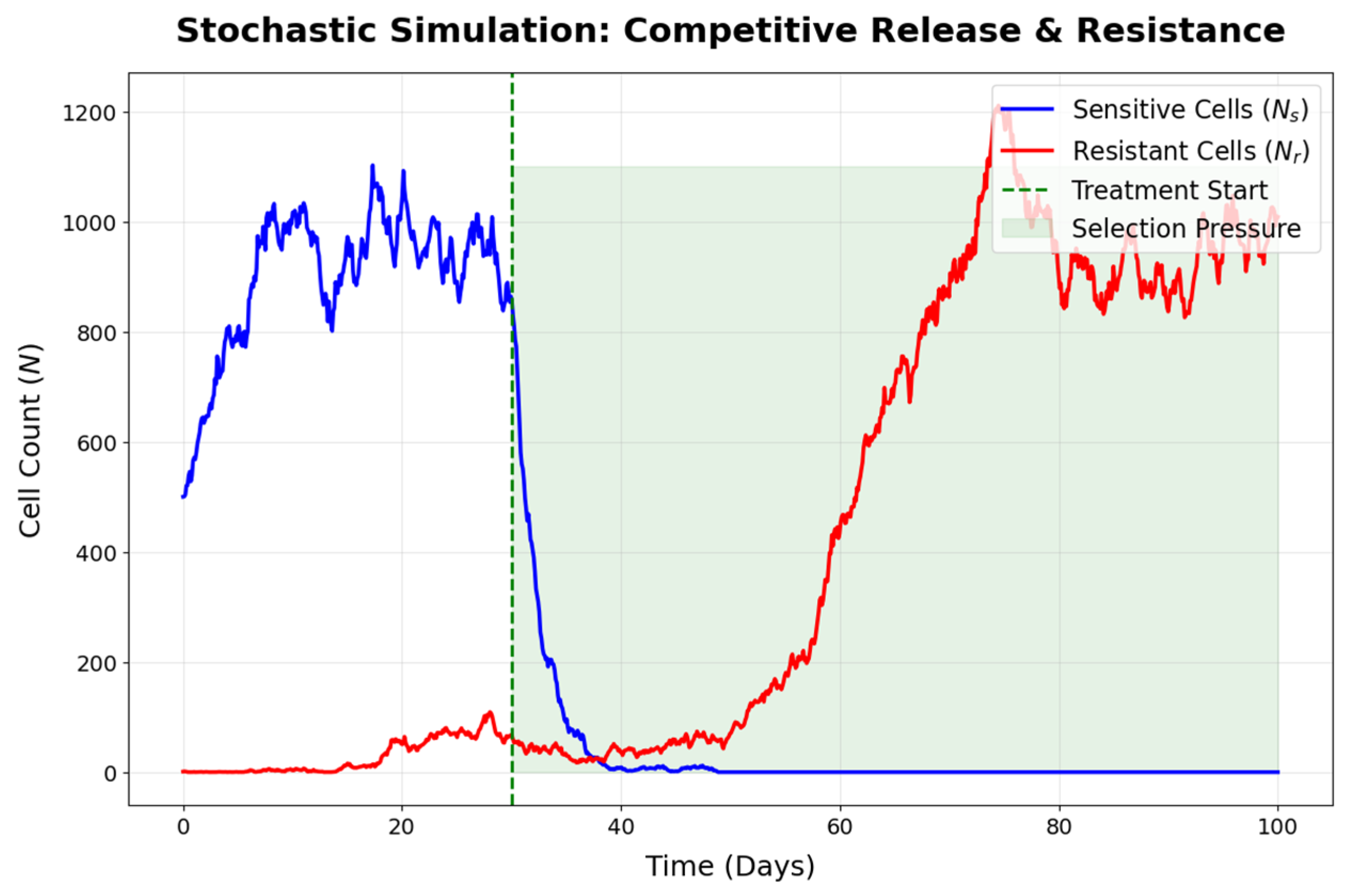

Disclaimer/Publisher’s Note: The statements, opinions and data contained in all publications are solely those of the individual author(s) and contributor(s) and not of MDPI and/or the editor(s). MDPI and/or the editor(s) disclaim responsibility for any injury to people or property resulting from any ideas, methods, instructions or products referred to in the content. |
© 2026 by the author. Licensee MDPI, Basel, Switzerland. This article is an open access article distributed under the terms and conditions of the Creative Commons Attribution (CC BY) license.