


Abstract
This manuscript introduces a new two-parameter discrete distribution derived from the binomial distribution by assuming that its success probability follows the Laplace-logistic unit (LLU) distribution. The resulting binomial Laplace-logistic unit (BLLU) distribution is studied in detail, including its probability mass function, cumulative distribution function, moments, dispersion, asymmetry, modality, and limiting behaviour. In particular, the convergence of the normalized BLLU random variable to the underlying LLU mixing distribution as the binomial parameter increases is established. Three parameter estimation procedures are considered, including the method of moments, maximum likelihood, and a quantile-based method for large values of the binomial parameter. Their finite-sample performance is investigated by means of a Monte Carlo simulation study. Finally, the applicability of the proposed distribution is illustrated through fitting to empirical environmental and traffic accidents count data.
Keywords:
binomial mixture; discrete distributions; Laplace-logistic unit distribution; parameter estimation; count data; applications MSC:
60E05; 62E10; 62F10
1. Introduction
Discrete random variables with bounded support arise naturally in many applications where the number of occurrences of an event is recorded over a fixed number of trials. The binomial distribution is therefore one of the fundamental models for bounded count data. However, its classical formulation assumes a fixed probability of success, which may be restrictive in heterogeneous populations or when the underlying success probability varies across experimental units. A natural extension is obtained by treating the binomial success probability as a random variable on the unit interval. Such models provide a flexible framework for bounded count data and allow additional variation to be introduced through the heterogeneity of the latent success probability, and have been studied by several authors. For instance, the beta-binomial distribution [1] represents the classical example of this construction, while alternative mixing distributions, including the Kumaraswamy distribution [2], have also been considered. More recently, related constructions have continued to appear in the literature. Thus, Irshad et al. [3] introduced a binomial mixture Lindley distribution, Chesneau et al. [4] proposed a binomial-discrete Poisson–Lindley distribution, and Azimi et al. [5] considered a logLindley-binomial and ordinal random effects model. Some recent works [6,7,8,9] have also considered flexible extensions for binomial mixture distributions and illustrate that the choice of the mixing distribution can lead to substantially different binomial mixture families.
In parallel, flexible probability distributions on the unit interval have become an attractive area of statistical research, motivated by applications involving proportions, probabilities, and other bounded continuous quantities (for some recent ones, see, e.g., [10,11,12,13,14,15,16]). In particular, the developments in the field of unitary continuous distributions are summarized by Afuecheta et al. [17]. Within this framework, Stojanović et al. [18] introduced the Laplace-logistic unit (LLU) distribution, a two-parameter distribution on obtained by a generalized logistic transformation of the Laplace distribution. The LLU distribution exhibits considerable flexibility with respect to symmetry, modality, and boundary behaviour, while its explicit quantile function also permits convenient parameter estimation together with an analysis of the corresponding asymptotic properties.
Motivated by the flexibility of the LLU distribution with respect to asymmetry and boundary behaviour, we consider it as a mixing distribution for the binomial success probability and derive the resulting discrete family in explicit form. Specifically, if and , the resulting marginal distribution, referred to as the binomial Laplace-logistic unit (BLLU) distribution, is a new discrete family supported on . The BLLU distribution offers a new binomial mixture based on the LLU distribution, combining the flexibility of continuous mixing with a rich analytical structure. Unlike the beta and Kumaraswamy mixing distributions, which lead to the beta-binomial and Kumaraswamy–binomial families, respectively, the LLU distribution provides a different parameterization of heterogeneity on the unit interval. The resulting BLLU model inherits the shape characteristics of the LLU density, allowing the binomial mixture to accommodate a range of symmetric and asymmetric probability mass configurations. In particular, the possibility of trimodal shapes, including configurations with modes at both support boundaries and an additional interior modal region, is illustrated in Section 2.7. Beyond introducing another member of the binomial-mixture family, the contribution of the present work lies in establishing a detailed set of distributional characterizations and developing three estimation procedures, including a quantile-based approach motivated by the mean-square convergence of the normalized BLLU variable to its latent mixing probability. Finally, the BLLU distribution is applied to two real-world datasets: weekly counts of days with sulfur dioxide (SO2) concentrations above 20 , and monthly counts of days with at least one fatal road traffic accident, both obtained from the Serbian Open Data Portal.
The remainder of the paper is organized as follows. In the next section, Section 2, the BLLU distribution is introduced and its main probabilistic properties are established. The subsequent section, Section 3, considers parameter estimation and the corresponding Monte Carlo simulation study, while applications of the proposed distribution are presented in a later section, Section 4. The paper concludes with some final remarks given in Section 5.
2. BLLU Distribution. Definition and Key Properties
Let Y be a random variable having the Laplace–Logistic Unit (LLU) distribution with parameters . Thus, its probability density function is defined on the unit interval as follows (see, for more detail, [18]):
It is easy to show that the density given by Equation (1) is continuous and normalized on , i.e., for all , the equality holds. Now, we define a new discrete distribution by considering the binomial model conditionally on the random success probability , i.e.,
The resulting marginal distribution of X will be referred to as the binomial Laplace-logistic unit distribution, or the BLLU distribution for short. Thus, for , the probability mass function (PMF) of the BLLU distribution is as follows:
The BLLU distribution is therefore a binomial mixture whose mixing distribution is the LLU distribution, and its basic stochastic properties are discussed below.
2.1. Probability Mass Function
The following statement gives an explicit representation of the PMF of the BLLU distribution.
Theorem 1.
Let X have the BLLU distribution, with and parameters . Then, for ,
where
and is an incomplete beta function.
Proof.
According to Equations (1) and (2), and using two branches of the LLU density with , one obtains:
Since is a nonnegative integer, the binomial formula gives:
and, consequently,
where
For the first integral, let . Then and the convergence implies Therefore,
For the second integral, the same substitution implies
so with the new substitution , we get:
Finally, substituting the obtained expressions for and into Equation (5) yields Equation (3), which completes the proof. □
Remark 1.
Although the second shape parameter in the incomplete beta functions appearing in Equation (4) may be negative, the corresponding integrals are nevertheless finite. Indeed, in the integral representation:
the factor is bounded for every fixed real b, provided that and . Consequently, the integrand is bounded by a constant multiple of , which is integrable at zero whenever . Thus, is finite for every real b. Note that in Equation (4), the upper integration limit is , while the first shape parameters are and λ, both strictly positive for and . Hence, both incomplete beta integrals are well-defined and finite, irrespective of the signs of their second shape parameters. For numerical evaluation, Equation (3) can be complemented by equivalent integral representations, given by Equation (2) or, using the quantile function of the LLU distribution, through the equivalent representation:
which can be approximated numerically by quadrature. A numerical comparison of the finite-sum and integral representations is provided in Supplementary Note S1.
Finally, the representation in Equation (3) also provides a way to formulate the identifiability condition for the BLLU family. Let , , with . These quantities are the raw moments of the LLU mixing distribution, as shown in Equation (12) below. Equation (3) can then be written as:
and for fixed n, this relation defines an invertible triangular transformation between the vectors and . Consequently, identifiability of the BLLU family is equivalent to injectivity of the mapping The numerical assessment of the first two moments, which is relevant to the method-of-moments procedure, is presented in Section 3.1.
Remark 2.
The normalization of the PMF of the BLLU distribution follows directly from its mixture construction. Indeed, according to Equations (1) and (2), it follows:
Hence, the support of the BLLU distribution is the set the same as for the binomial distribution. It is also useful to observe that the function , defined by Equation (4), has an alternative integral representation. For that purpose, in the first integral, given by Equation (6), we use the substitution and in the second one, given by Equation (7), first put and then use the same transformation. After some straightforward calculations, one obtains:
which is useful for studying the properties of the BLLU distribution that follow below. Furthermore, note that the integral in Equation (8) converges for all , , and . Indeed, when , its integrand is asymptotically proportional to , whereas the remaining factor has a finite limit as .
2.2. Cumulative Distribution Function
The following statement explicitly gives the cumulative distribution function (CDF) of the BLLU distribution.
Theorem 2.
Let X have the BLLU distribution, whose PMF is given by Equation (3), and let . Then, the CDF of X is given by:
Proof.
Starting from Equation (3) and using the substitution , we obtain:
From here, using the combinatorial identity:
we may write:
and, therefore,
Note that for , the inner sum is:
and for , it is equal to 1. Finally, for , using Pascal’s identity:
the partial alternating binomial sum can be evaluated as:
From here, multiplication by gives:
and, consequently,
Finally, when , Equation (8) gives:
so the first term in Equation (10) is equal to 1, and Equation (9) immediately follows. □
2.3. Probability Generating Function
The probability generating function (PGF) of the BLLU distribution is defined as . The following statement expresses this function in explicit form.
Theorem 3.
Let X have the BLLU distribution. Then, its PGF is given by the equality:
where is defined by Equation (4).
Proof.
Conditionally on , the random variable X follows a binomial distribution, i.e.,
Taking the expectation with respect to Y, and applying the binomial theorem, one obtains:
According to Theorem 1 (see, also, Theorem 2 in [18]), it follows:
which proves Equation (11). □
Remark 3.
Since the BLLU distribution has finite support, its PGF is a polynomial of degree at most n. Therefore, it is finite and well defined for every (in fact, for every ). Thus, although PGFs are often considered on the standard domain , no such restriction is necessary for the BLLU distribution. In particular, according to Equation (11), the equality holds. Thus, differentiation the PGF at yields the factorial moments of the BLLU distribution, described below.
2.4. Factorial and Ordinary Moments
Let denote the falling factorial, with . Then, the following statement is valid:
Theorem 4.
For , the rth factorial moment of the BLLU distribution is
where
Proof.
As is known, the rth derivatives of the PGF satisfy equality for arbitrary . Hence, differentiating Equation (11) r times gives:
Obviously, all terms with vanish at , while for ,
Therefore,
which proves the result. □
Using the previous theorem, i.e., the factorial moments obtained above, the ordinary (raw) moments of the BLLU distribution can be expressed. First, recall that:
where
denotes a Stirling number of the second kind (see, e.g., [19]). Hence, using Equation (13), one obtains:
where are the ordinary moments of the mixing LLU distribution, given by Equation (12).
2.5. Mean and Variance
Using Equation (14), the mean and variance of the BLLU distribution can be expressed, respectively, as follows:
and
Here, denotes the binomial random variable with the probability parameter . Hence, the variance of the BLLU distribution consists of two components: the first term corresponds to the usual binomial contribution, whereas the second term is induced by the variability of the LLU mixing distribution.
Using Equations (15) and (16) and , the dispersion index of the BLLU distribution can be expressed as follows:
where
are the dispersion indices of the random variables Y and Z, respectively. Note that for the contribution of mixing heterogeneity to the dispersion index vanishes, and coincides with the Bernoulli dispersion index . Conversely, since and , it follows that, for fixed ,
Moreover,
Thus, for every , the BLLU distribution has a larger dispersion index than its LLU mixing distribution.
The growth of the dispersion of the BLLU distribution with an increase in the binomial parameter n can be further characterized. For , we get:
or, equivalently,
Consequently, for every fixed , there exists a finite integer such that:
Thus, although the BLLU distribution need not be overdispersed for every finite n, its dispersion index eventually exceeds one and grows without bound as n increases.
2.6. Location and Asymmetry
The shape of the BLLU distribution is determined by the interaction of the mixing distribution and the binomial sampling mechanism. Recall that:
where , and . As will be shown here, the parameter primarily controls the direction of asymmetry inherited from the mixing LLU distribution, whereas affects the concentration and the amount of heterogeneity of the random success probability Y. In addition, the integer parameter n controls the level of aggregation of the latent probability Y into the discrete variable X. Consequently, the discrete shape of the BLLU distribution may be substantially richer than the shape of the corresponding continuous mixing distribution.
As is shown in [18] (Thm. 4), the LLU distribution is symmetric for , positively asymmetric for , and negatively asymmetric for . Moreover, its mode is located at distinguished point whenever the corresponding unimodality conditions are satisfied. Hence, the first indication of the role of the parameter in the shape properties of the BLLU distribution is obtained from its mean value. According to the standard mean formula for a binomial mixture, given by Equation (15), one obtains:
Thus, the location of the BLLU distribution relative to the center of its support is determined entirely by and is independent of n. It is therefore useful to define the mean-position index:
so that the sign of is the same as the sign of . In a more formal way, using the third moment, the asymmetry of the BLLU distribution can be expressed as follows.
Theorem 5.
Let and let denote the third central moment of X. Then,
i.e., the BLLU distribution has the same direction of moment skewness as the corresponding LLU mixing distribution. Furthermore, the BLLU distribution is symmetric about if and only if .
Proof.
Using Equation (13), the first three raw moments of the BLLU distribution can be obtained from the factorial moments representation as:
where , denote the first three raw moments of the LLU distribution. Substituting the above expressions into the definition of the third central moment yields:
where is the third central moment of Y. Since , , and , the last equality gives:
At the same time, by Equation (18), , and since , the first term in Equation (19) has the sign of whenever . Further, the second term has the same sign whenever its coefficient is nonzero. Finally, using the established LLU property and , the third term has the same sign whenever its coefficient is nonzero. Thus, all nonzero terms in Equation (19) have the same sign, which proves the asserted sign of . Furthermore, using the quantile function of the LLU distribution given by Equation (14) in [18], the following stochastic representation holds:
where and is symmetric. By the convex-transformation result of van Zwet [20] (Thm. 2.2.1), the third standardized central moment is positive for and negative for , since the corresponding power transformations are strictly convex and increasing.
It remains to establish exact symmetry. For , it can be easily seen that the LLU density, defined by Equation (1), satisfies (see, also [18] (Remark 4)):
Consequently, for every , Equation (2) gives:
Thus, the BLLU distribution is symmetric when . Conversely, suppose that the BLLU distribution is symmetric about . Then, and, therefore, From the characterization of , this is possible only for . Hence, the BLLU distribution is symmetric if and only if . □
Remark 4.
The decomposition in Equation (19) provides a useful interpretation of the third central moment of the BLLU distribution. In particular, the first term in Equation (19) is exactly the third central moment of a binomial distribution , and represents the skewness induced by the binomial sampling mechanism at the average success probability . The second term reflects the additional contribution caused by the heterogeneity of the random success probability Y, whereas the third term directly transfers the third central moment, and hence the direction of moment skewness of the LLU mixing distribution. Thus, the skewness of the BLLU model results from the combined effect of these three components, but also depends on . For , the BLLU distribution reduces to a Bernoulli distribution with parameter , and only the first (binomial) component is present. For , the third contribution vanishes, while the first two components remain. Finally, for , all three components may contribute to the skewness.
2.7. Modality
Unlike symmetry and mean location, the modality of the BLLU distribution cannot, in general, be characterized by a simple closed-form expression for the mode. This is a consequence of the binomial mixture structure:
which combines the shape of the mixing density with the discrete binomial kernel. More generally, for any valid mixing density on , the resulting binomial mixture has at least one global mode, since its support is finite.
A convenient way to investigate the modality is to consider the ratio of successive probabilities:
Hence, an interior point is a local mode whenever:
Similarly, the lower boundary point is a local mode if and only if , and since:
this condition is equivalent to:
Analogously, is a local mode if and only if , that is,
These relations provide precise criteria for identifying boundary modes, and the following result further links the modal behaviour of a BLLU distribution to its LLU mixing density.
Theorem 6.
Let follow the BLLU distribution with binomial parameter n and mixing density . Then,
where is a random variable with beta distribution. Consequently:
- (i)
- If is non-increasing on , then i.e., is a mode of the BLLU distribution.
- (ii)
- If is non-decreasing on , then i.e., is a mode of the BLLU distribution.
Proof.
As is known, the random variable has the density (see, e.g., [21] (Ch. 25))
where denotes the beta function. Further, and are non-negative integers, so using the well-known relation between the beta and gamma functions, one obtains:
and hence:
From this obtained density , the PMF of the BLLU distribution, given by Equation (2), can be rewritten as follows:
which proves the stated representation in Equation (21). Moreover, the ratio:
is strictly increasing in , and hence the family is ordered in the monotone likelihood-ratio sense. Since the likelihood-ratio order implies the usual stochastic order (see, e.g., [22]), we obtain for any Thus, by the defining property of the stochastic order, if density is non-increasing, then:
while non-decreasing density implies:
According to Equation (21), it follows that for a non-increasing mixing density , and for a non-decreasing mixing density, which completes the proof. □
The preceding theorem provides a direct link between the shape of the LLU mixing density and the modality of the BLLU distribution. In particular, according to the results established for the LLU distribution in [18] (Thm. 1), the LLU density is decreasing when:
and increasing when:
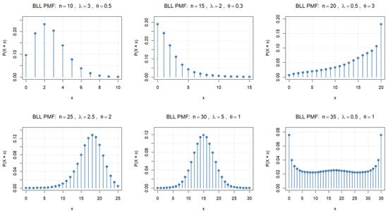
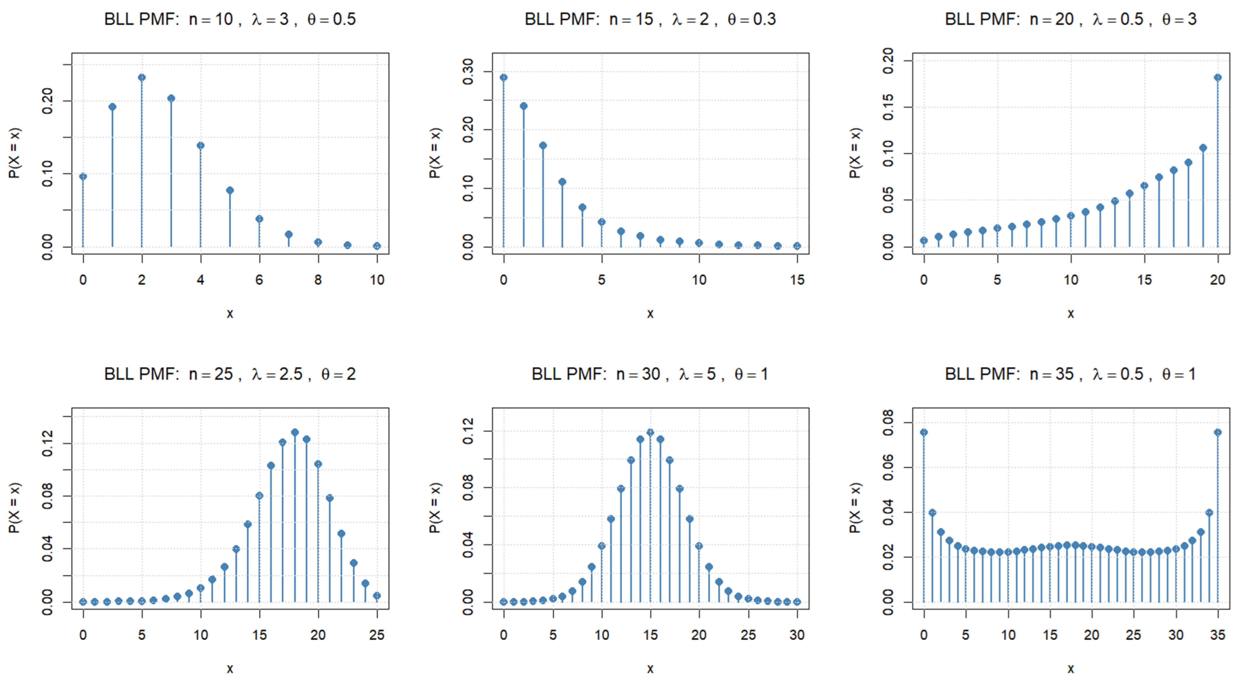
By Theorem 6, these conditions also guarantee, respectively, a decreasing BLLU PMF with a mode at and an increasing BLLU PMF with a mode at . The second and third panels of Figure 1 below illustrate these two cases, with parameter configurations and , respectively.
Figure 1.
Some representative shapes of the BLLU probability mass function for selected values of , , and n.
In addition, a particularly important case arises when the LLU mixing density is unimodal, i.e., has an interior local maximum. According to the results established for the LLU distribution [18] (Thm. 4), this maximum is located at whenever and For the corresponding BLLU distribution, the mode does not generally admit a simple closed-form expression for finite n. Nevertheless, its location may be related asymptotically to the mode of the underlying mixing density. To this end, let be any sequence of non-negative integers such that:
From the beta representation given by Equation (21), it follows:
at every interior continuity point t of the mixing density . This convergence motivates the following conjecture: when the mixing density has a unique interior global mode and its boundary behaviour does not dominate the interior contribution, the modes of the corresponding BLLU distributions satisfy:
Establishing this mode-convergence statement rigorously would require additional assumptions ensuring suitable uniform control of the rescaled PMF near the unique interior mode. Hence, this statement is a conjecture rather than a proved result, since pointwise convergence alone does not guarantee convergence of the global modes. It nevertheless provides a natural link between the continuous mixing distribution and the discrete shape of the BLLU model, which will be illustrated further below.
The parameter further determines the asymptotic modal location through the asymmetry of the LLU mixing distribution. In the symmetric case , the identity holds for all , so any interior mode is accompanied by a symmetric counterpart. Depending on the values of and n, the BLLU distribution may consequently exhibit symmetric bimodal or trimodal configurations. For , this symmetry is lost, and asymmetric multimodal configurations may also arise. The parameter further affects the concentration of the mixing distribution, particularly near the boundaries of . Overall, the BLLU family is capable of exhibiting a wide range of discrete shapes, from monotone, unimodal and multimodal to symmetric and asymmetric forms, as is shown in Figure 1.
The first three panels in Figure 1 demonstrate how the parameter determines the direction and degree of asymmetry. For , as shown in the first two panels, the probability mass is concentrated toward the lower part of the support, resulting in positively skewed distributions. In contrast, the third panel, with , exhibits a pronounced negative skewness, with probability mass concentrated toward the upper boundary .
The lower panels further illustrate the joint effect of and on the shape of the distribution. The case produces a strongly asymmetric distribution with a mode located away from the center and substantial concentration in the upper part of the support. When , the symmetry property established above is clearly visible. For , the distribution is centrally concentrated and unimodal, with a central mode at . Unlike many other binomial mixtures, the BLLU distribution can be trimodal, as is the case for . In this instance, it is highly dispersed, with boundary modes at and , as well as a central modal plateau at . Note that for this parameter configuration, and hold, so according to Theorem 1 in [18], the LLU density is two-tailed. Further, the conditions for an interior local maximum in Theorem 4 of the same reference are satisfied, since and . Direct numerical evaluation of the BLLU PMF confirms the three modal peaks, with the central peak comprising two adjacent values of equal probability.
2.8. Asymptotic Properties
The asymptotic behaviour of the BLLU distribution can be described using two complementary aspects that are formulated by the following statements.
Theorem 7.
Let denote a sequence of BLLU random variables with parameters , and Then,
where denotes the mean squared convergence.
Proof.
Conditional on Y, we have and therefore:
According to this, using the expectation of conditional variance, one obtains:
Since (a.s.), it follows that Hence,
which confirm the convergence in Equation (22). □
Remark 5.
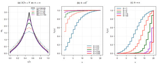
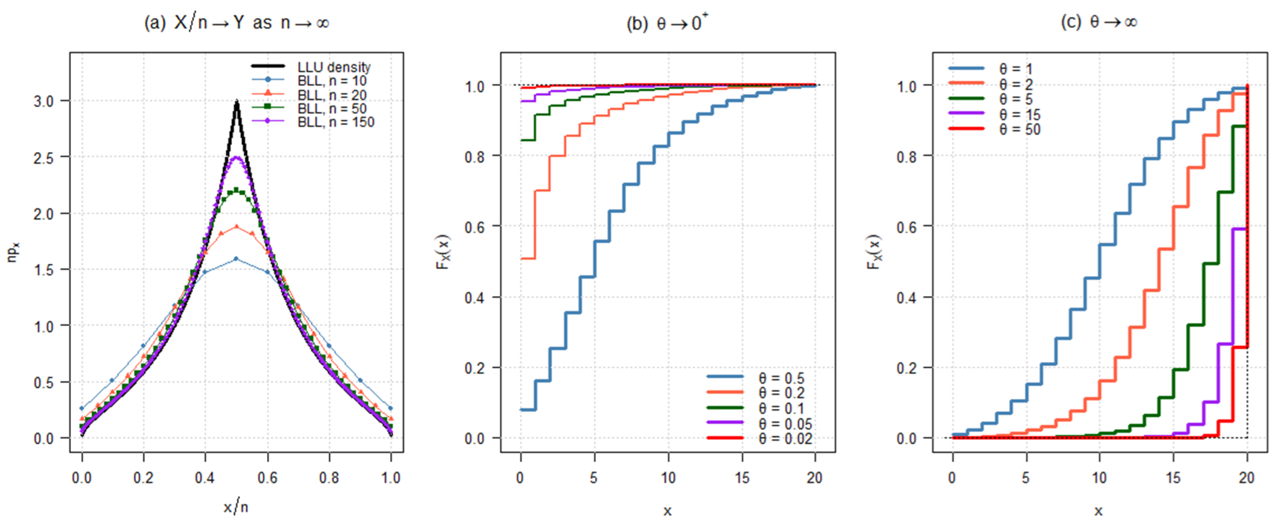
The preceding result has a natural interpretation: as the binomial size n increases, the normalized random variable approaches the latent success probability Y, and the BLLU distribution asymptotically recovers its LLU mixing distribution. In this sense, the normalized BLLU distribution provides an asymptotically exact discrete representation of the underlying LLU distribution, as shown in Figure 2a, below. The same conclusion is also reflected by the first two moments. Namely, according to Equation (15), for every ,
and according to Equation (16):
Thus, it follows:
Figure 2.
Asymptotic behaviour of the BLLU distribution: (a) Convergence of the normalized BLLU distribution to the LLU mixing distribution as . (True parameters are: , ). (b,c) Concentration of the BLLU distribution at as , and as , illustrated by the corresponding CDFs, with several values of , while and .
Theorem 8.
Let , with fixed and . Then,
Proof.
We use the stochastic representation of the LLU distribution given by Equation (20). Since (a.s.), in the limit case when , we have:
Hence, the bounded convergence theorem gives (see, e.g., [23] (Thm. 16.5)):
Further, using the conditional moments of the binomial distribution, one obtains:
Therefore,
which confirms the first convergence in (23).
Next, let . Then, we have:
and re-applying bounded convergence gives:
Consequently, since:
and, by the law of total variance (see, e.g., [24] (Thm. 12.2.6)),
it follows that:
Hence, the second convergence in (23) is also confirmed. □
Remark 6.
Preceding theorem indicates that the parameter θ determines the direction of concentration of the BLLU distribution across its support. In particular, using the stochastic representation of the LLU mixing distribution, given by Equation (20), we have proven that as , the latent success probability converges to zero, whereas as , it converges to one. Consequently, convergences in Equation (23) imply the following convergences in distribution:
Equivalently, the corresponding distributions converge weakly to degenerate distributions and , concentrated at and , respectively. Figure 2b,c show the convergence of the CDFs of these distributions, for several values of θ. As is well known, convergence in distribution is characterized by the convergence of CDFs at the points of continuity of the boundary CDF, and together with the symmetry result at , provide a direct interpretation of θ as a parameter governing the direction of the concentration of the BLLU distribution over its support.
3. Parameter Estimation and Simulation Study
This section considers three approaches to the parameter estimation of the BLLU distribution. The proposed procedures are based on three different characteristics of the model. The first one exploits the factorial moment structure induced by the binomial mixture and leads to method-of-moments (MoM) estimators. The second procedure is based on maximum likelihood estimation (MLE) and uses the complete probability mass function of the BLLU distribution. Finally, a quantile-based procedure is considered for large values of the binomial parameter n, motivated by the asymptotic relationship between the normalized BLLU distribution and its LLU mixing distribution.
To that purpose, let be an independent random sample from distribution, where n is assumed to be known and Thus, the observations are generated according to The three estimation procedures considered below have complementary motivations. The MoM takes advantage of the particularly simple relationship between the factorial moments of the BLLU random variable and the ordinary moments of its mixing distribution. MLE uses the complete BLLU probability mass function and therefore incorporates all distributional information contained in the sample. Finally, the third procedure is specifically designed for large values of n and is based on the convergence given by Equation (22). All three approaches are described in more detail below.
3.1. Method of Moments
Let denote the rth raw moment of the LLU mixing distribution, given by Equation (12). According to Equation (13), the factorial moments of satisfy:
where denotes the falling factorial. In particular,
and for an observed sample the empirical counterparts of and are obtained directly from the BLLU observations as:
where it is assumed that and is the sample mean.
The MoM estimators are therefore obtained by matching the first two empirical factorial moments of the observed BLLU sample with their theoretical counterparts. Using the identities above, they are defined as the numerical solution of the coupled equations:
In finite samples, a convenient numerical implementation is to minimize the moment discrepancy:
Note that the use of the LLU moments does not require observations from the mixing distribution. Rather, it provides a convenient representation of the BLLU factorial moments, given by Equation (24), which reduces the BLLU moment estimation problem to the corresponding moment functions of the LLU mixing distribution. Further, under identifiability of the mapping:
and the usual continuity and regularity conditions (see, e.g., [25]), the law of large numbers (LLN) implies:
To assess the local identifiability of the moment mapping, we evaluated the Jacobian determinant with respect to on a logarithmic grid over , and the determinant was positive at all grid points. These numerical diagnostics support local identifiability of the two-moment mapping in the investigated parameter region, but do not establish global injectivity (see Supplementary Note S2). Accordingly, the consistency of the MoM estimators is conditional on identifiability of the moment mapping and the usual regularity conditions. Their finite-sample behaviour, including the variability of the resulting estimates, is investigated through the Monte Carlo study below.
3.2. Maximum Likelihood Estimation
Let , with , denote the PMF of the BLLU distribution, obtained through Equation (2) from the definition of the model. For an observed BLLU sample , the corresponding likelihood function is:
and the corresponding log-likelihood function is:
Equivalently, if , , denotes the observed frequency of the value x, where is an indicator of the event , then:
Thus, the log-likelihood depends on the sample only through the observed frequencies .
The ML estimators and are defined as the values of that maximize the log-likelihood function, i.e.,
Note that unlike the MoM procedure, MLE uses the complete BLLU probability mass function. Consequently, the evaluation of the likelihood requires the computation of the probabilities , which can be obtained directly from the explicit representation in Equation (3). Alternatively, the integral representation in Equation (2) may be evaluated numerically. The resulting log-likelihood is then maximized numerically over the positive parameter space, where the MoM estimates are used as initial values for the likelihood maximization.
This choice provides a natural computational strategy, since the moment estimators can be obtained relatively quickly and typically provide parameter values in a reasonable neighborhood of the likelihood optimum. Similar to MoM estimators, under the usual identifiability and regularity conditions for parametric models, MLE estimators possess the standard large-sample properties, including consistency and asymptotic normality (see, e.g., [26]). Establishing these properties rigorously for the BLLU model would require a separate analysis of the regularity of the mixture likelihood and is beyond the scope of the present work. Accordingly, the performance of the maximum likelihood procedure is assessed here through the Monte Carlo simulation study presented below.
3.3. Large-n Quantile Estimation
The third estimation procedure is motivated by the large-n behaviour of the BLLU distribution. As established in the preceding section, i.e., in Equation (22), for large values of n, the distribution of the normalized BLLU random variable is approximated by the corresponding random variable Y from LLU mixing distribution. Hence, for an observed BLLU sample , define the normalized observations by , . The resulting observations take values on the grid and provide a discrete large-n approximation to a sample from . This suggests applying the quantile-based estimation procedure, developed for the LLU distribution, which is applied here to the normalized BLLU observations.
Let , , denote the quantile function of the LLU distribution. Its two branches are given by (see, for more detail [18]):
A particularly useful property of the LLU quantile function is that its median does not depend on , that is,
Therefore, if denotes the empirical median of the normalized observations , a natural large-n estimator of is:
Once has been estimated, the parameter is estimated using the first and third empirical quartiles of the normalized observations, denoted by and , respectively. From the explicit form of the LLU quantile function, given by Equation (27), it follows that:
Consequently, substituting the empirical quartiles and the estimator yields
Thus, both parameters are estimated directly from the empirical median and quartiles, without numerical optimization.
Note that the proposed quantile procedure exploits the explicit quantile structure of the LLU mixing distribution after normalization of the BLLU observations. Its principal computational advantage is that it avoids repeated numerical evaluation within an optimization procedure. Furthermore, this procedure is based on the large-n relationship between the BLLU distribution and its LLU mixing distribution. According to the convergence given by Equation (22), the quantile-based estimation methodology provides a natural basis for the estimation of the BLLU parameters from the normalized observations , . For fixed n, however, increasing N alone does not generally eliminate the discrepancy between the quantiles of and those of the LLU distribution. In particular, as , the empirical quantiles converge to the corresponding quantiles of the BLLU distribution, so applying the LLU quantile inversion generally leads to pseudo-true parameter values rather than necessarily to the underlying parameters. Writing , for , and using the proof of Theorem 7, we obtain the identity:
Consequently, the mean-square approximation error decreases at rate , which quantifies the approximation underlying the large-n quantile estimation procedure. Accordingly, the proposed procedure should be interpreted as a large-n approximation, and its finite-sample performance is investigated in the Monte Carlo study presented in Section 3.4. A further assessment of the approximation error and the sensitivity of the quantile-based estimator to the binomial parameter n and the selected quantile pair are further examined in Supplementary Note S3.
Remark 7.
The three estimation procedures exploit different structural features of the BLLU model. The MoM is based on the factorial moment identity induced by the binomial mixture, whereas MLE uses the complete BLLU probability mass function. In contrast, the quantile procedure is based on the asymptotic relationship between the normalized BLLU random variable and its LLU mixing distribution. Consequently, these three methods are motivated by different aspects of the model. The MoM is computationally simple and uses a small number of summary characteristics of the distribution, while MLE uses the complete distributional information at the cost of repeated probability evaluation and numerical optimization. Finally, the quantile procedure provides an alternative that is particularly attractive for large n, where the normalized BLLU distribution is well approximated by the corresponding LLU distribution.
3.4. Monte Carlo Simulation Study
The finite-sample performance of the three proposed estimation procedures is investigated by means of a Monte Carlo simulation study. In particular, the MoM, MLE, and the proposed large-n quantile procedure are examined in terms of their empirical mean, bias, standard deviation (SD), root mean squared error (RMSE), and approximate normality of the estimators. Furthermore, in order to represent substantially different shapes and regimes of the BLLU distribution, three different parameter configurations are considered:
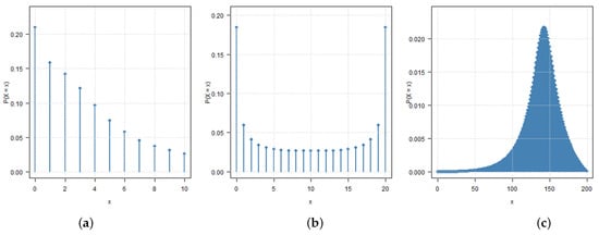
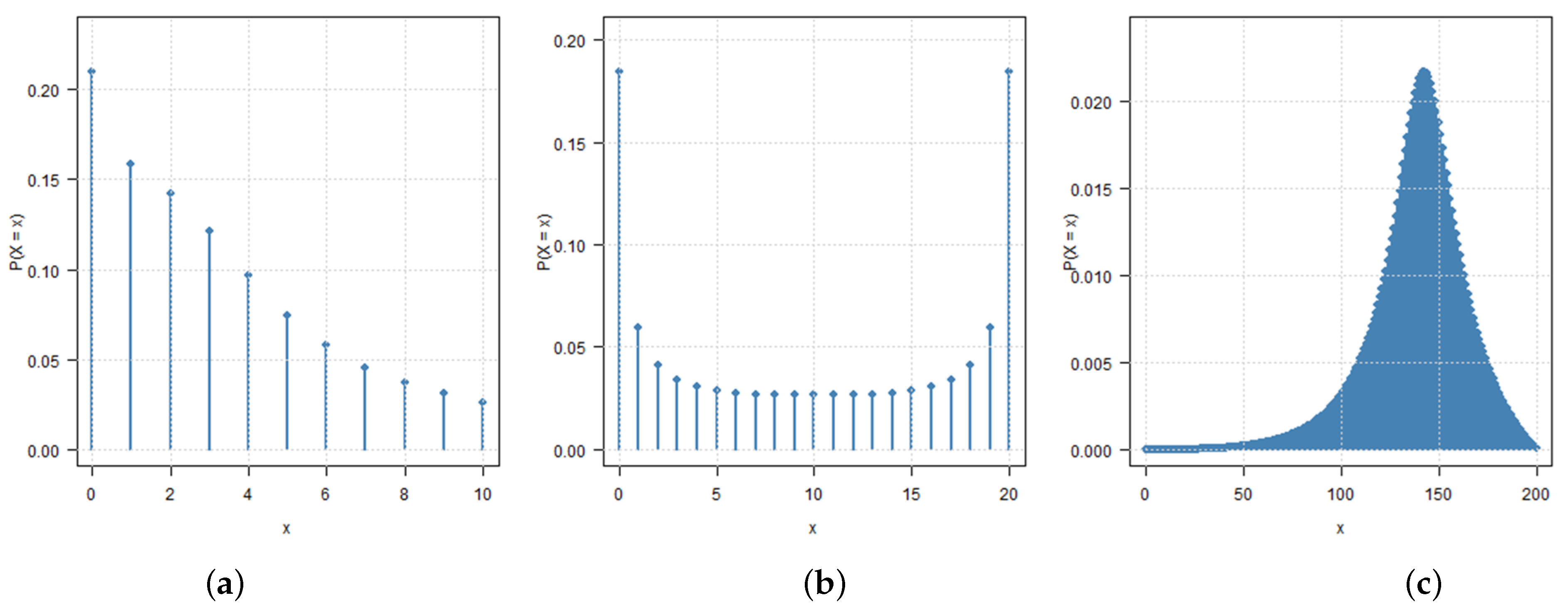
The first configuration represents a positively asymmetric, decreasing BLLU distribution, with a relatively small value of the binomial parameter n. Conversely, the second configuration corresponds to the symmetric case and exhibits a pronounced concentration of probability near the boundaries of the support. Finally, the third configuration represents a negatively asymmetric distribution in the large-n regime. In this context, the MoM is considered under all three configurations, while the MLE is compared with MoM in Scenarios I and II using identical simulated samples. The quantile-based procedure is primarily investigated in Scenario III, where its large-n theoretical justification applies. Its behaviour under the two small-n configurations is additionally examined as a diagnostic assessment, with the corresponding results reported in Supplementary Note S3.
For the MoM procedure, the moment-discrepancy objective function in Equation (25) is minimized using the optim() routine in R (version 1.0-4) with the Nelder–Mead simplex algorithm [27]. For the MLE procedure, implemented in Scenarios I and II, the negative log-likelihood corresponding to Equation (26) is minimized using the L-BFGS-B algorithm on the log-parameter scale, with . The control settings were maxit = 600, factr = , and pgtol = . Three starting values were used for each sample: the method-of-moments estimates and two fixed initial pairs, and . In this context, only solutions with finite objective values and a zero optimizer convergence code were accepted, and the solution with the highest log-likelihood was retained. Further details and likelihood-surface diagnostics are provided in Supplementary Note S4. Finally, the third scenario is particularly motivated by the large-n convergence of the normalized BLLU variable to its LLU mixing distribution. Hence, using the previous results on LLU parameter estimation [18], natural estimation approach is based on the quantile procedure, described in the previous section, i.e., by the simple use of Equations (27)–(29). The PMFs corresponding to the selected parameter configurations are displayed in Figure 3.
Figure 3.
PMFs of the BLLU distribution for the three parameter configurations considered in the Monte Carlo simulation study: (a) ; (b) ; and (c) .
Regarding numerical evaluation, note that although Equation (3) provides an explicit finite-sum representation of the BLLU probability mass function, its alternating terms may cause loss of numerical precision for moderate or large values of n. Therefore, the accompanying R implementations use alternative numerical approaches. In the direct PMF calculation, the integral in Equation (2) is evaluated separately over and , where , using R’s adaptive integration routine with relative tolerance . In the MLE simulation code, the equivalent quantile-based integral representation is approximated by the midpoint rule using equally weighted points, and the resulting probability vector is normalized before evaluating the log-likelihood. In this way, both approaches avoid direct evaluation of the alternating sum in Equation (3), reducing the risk of cancellation-related numerical errors.
Further, for each experiment, independent samples of sizes are generated, and Monte Carlo replications are performed for each sample size. Additionally, the sensitivity of the main Monte Carlo summaries to the number of replications was assessed using cumulative prefixes of the first 100, 200, 250, and 300 replications and the results are reported in Supplementary Note S4. The BLLU observations are then generated according to the hierarchical representation of the model by first simulating the latent LLU random variable through its quantile representation and subsequently generating the corresponding binomial observation conditionally on the latent success probability. Further, the empirical distributions of the parameter estimates are examined by using the Shapiro–Wilk (SW) and Anderson–Darling (AD) tests of normality. For each estimator, both the corresponding test statistics and p-values are reported. To this end, in addition to the standard R-functions available in the stats package, the nortest package [28] was used for the AD test of normality, and for reproducibility, the random-number generator was initialized using set.seed(123) in R (version 1.5.1).
The Monte Carlo results reported in Table 1, Table 2 and Table 3 summarize estimator performance under the three parameter configurations, with direct comparisons to procedures evaluated on the same simulated samples. Table 1 and Table 2 present the results for Scenarios I and II, where the MoM and MLE procedures are compared using the same simulated samples within each replication. Further, Table 3 reports the results for Scenario III, comparing MoM with the large-n quantile-based procedure. According to the results thus obtained, the following observations can be made:
Table 1.
Monte Carlo summary statistics and normality tests for the MoM and MLE estimates of the BLLU parameters under Scenario I, with .
Table 2.
Monte Carlo summary statistics and normality tests for the MoM and MLE estimates of the BLLU parameters under Scenario II, with .
Table 3.
Monte Carlo summary statistics and normality tests for the MoM and large-n quantile estimates of the BLLU parameters under Scenario III, with .
- Under Scenario I, both MoM and MLE provide nearly unbiased estimates of , even for , whereas the estimates of exhibit a noticeable positive bias for the smallest sample size. At the same time, for both estimated parameters, the biases and RMSE values decrease as N increases. MLE yields somewhat lower RMSE values for throughout the considered sample-size range, while the two procedures perform very similarly for .
- A comparable pattern is also observed under Scenario II. The parameter is estimated relatively accurately even for smaller samples, whereas the estimation of exhibits substantially greater variability at . Nevertheless, it is obvious that both procedures improve as the sample size increases, so their performance is generally similar. MLE yields slightly lower RMSE values for at all considered sample sizes and for when . For , the two procedures perform almost identically for , with a marginally lower RMSE for MoM.
- Under Scenario III, the comparison between MoM and the quantile-based procedure reveals a parameter-dependent difference in performance. For , MoM yields lower RMSE values at every sample size, with its empirical bias becoming negligible at . Although the quantile-based estimator has a smaller absolute bias for the smaller and intermediate sample sizes, its RMSE remains higher and a negative bias is observed at . Conversely, for , the quantile-based procedure yields lower RMSE values than MoM at all four sample sizes. Thus, neither procedure uniformly outperforms the other for both parameters, but both show improved estimation precision as N increases.
Overall, the RMSE values decrease with increasing sample size N, indicating improved estimation precision for all procedures. SW and AD tests provide an empirical assessment of the normality of the simulated estimator distributions. Departures from normality are detected in several cases for smaller sample sizes, particularly for estimates of under Scenario I, estimates of under Scenario II, and the quantile-based estimates of under Scenario III. Although the results do not indicate a strictly monotonic improvement for every estimator as N increases, for neither test rejects normality for any of the estimator–parameter combinations considered. These findings provide numerical evidence consistent with an increasingly adequate normal approximation at larger sample sizes, without constituting a formal proof of asymptotic normality.
4. Applications of the BLLU Distribution
To illustrate the practical applicability of the proposed BLLU distribution, two real-world datasets from Serbia are considered. The first dataset consists of weekly sulfur dioxide (SO2) exceedance counts obtained from air-quality monitoring stations, while the second one is based on monthly counts of days with at least one fatal road traffic accident. The two datasets differ both in their field of application and in the binomial parameter, with for the SO2 data and for the traffic accident data. In both cases, the response variable is naturally interpreted as the number of days satisfying a specified condition among a fixed number of days in the corresponding observation period.
The proposed BLLU distribution is fitted along with three related competitive models, namely the ordinary binomial, beta-binomial, and Kumaraswamy–binomial distributions. Model performance is assessed using the maximized likelihood , Akaike Information Criterion (AIC), Bayesian Information Criterion (BIC), mean squared error (MSE) between the empirical and fitted probability masses, and discrete Cramér–von Mises (CVM) and Anderson–Darling (AD) goodness-of-fit criteria. All numerical calculations were performed in the R statistical software environment, whereby CVM and AD procedures are implemented within the dgof package [29]. To estimate the discrete goodness-of-fit, the CVM and AD statistics were computed based on the corresponding discrete formulations, with p-values obtained from 50,000 independent Monte Carlo samples under fitted null distributions. The R code, input datasets, and numerical details required to reproduce the discrete goodness-of-fit statistics and their Monte Carlo calibration are provided in Supplementary Note S5. Finally, the standard errors (SEs) of the MLEs were calculated from the inverse observed information matrix, obtained by numerically evaluating the Hessian of the negative log-likelihood at the MLEs. For positive-valued parameters, the calculations were performed on the log scale, and the resulting standard errors were transformed to the original parameter scale using the delta method. In this way, the reported SEs quantify the uncertainty associated with the estimated model parameters.
4.1. Application to Sulfur Dioxide Data
The first dataset consists of daily sulfur dioxide (SO2) concentration measurements recorded at air-quality monitoring stations in Serbia during the period 2011–2023. The data were obtained from publicly available environmental monitoring records provided by the Serbian Environmental Protection Agency (SEPA) through the Serbian Open Data Portal [30]. For each monitoring station and each seven-day period with complete daily observations, the variable X is defined as the number of days on which the observed SO2 concentration exceeded 20 . This threshold was selected in accordance with the 24-h guideline value specified in the World Health Organization (WHO) “Global Update 2005” [31], and applied consistently throughout the entire observation period. Hence, and the natural binomial parameter is fixed at .
Note that the annual data files for 2011–2023 yielded 16,744 potential station-week observations, based on 52 non-overlapping seven-day periods per year and the available monitoring stations. Of these, 15,163 had complete daily measurements for all seven days; the remaining 1581 incomplete station-week units were excluded without imputation. For the illustrative model-fitting analysis, a random sample without replacement of complete station-week observations (approximately of the eligible population) was selected. This sample size also helped keep the computational burden of the Monte Carlo calibration of the discrete goodness-of-fit tests manageable. The sample frequency distribution was broadly consistent with that of the complete station-week population.
The resulting empirical frequency distribution is given in Table 4, with sample mean and empirical variance Thus, the empirical variance significantly exceeds the sample mean, indicating overdispersion relative to the ordinary binomial model and providing empirical support for the additional mixing variability captured by the BLLU model.
Table 4.
Empirical frequency distribution of the weekly number of days with .
To assess the fitting performance of the proposed BLLU distribution, it is compared with three competing models: the ordinary binomial, beta-binomial, and Kumaraswamy–binomial distribution, whereas the parameters of all four models were estimated by MLE. In the case of the BLLU model, the numerical MLE maximization was initialized at the MoM estimates obtained from Equation (25). For the grouped observations in Table 4, the likelihood of each model is evaluated as:
where , and denotes the corresponding model probability for the unknown parameters . The resulting parameter estimates, fit statistics, and goodness-of-fit measures are summarized in Table 5.
Table 5.
Parameter estimates, fit statistics, and goodness-of-fit results for the competing models fitted to the SO2 data.
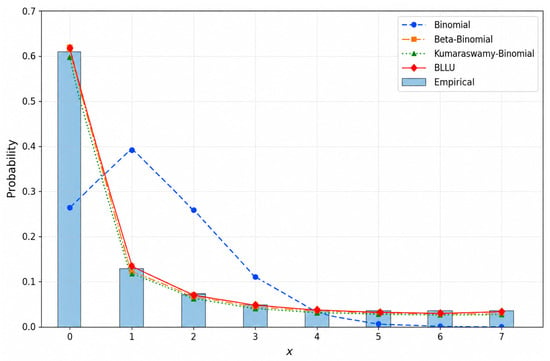
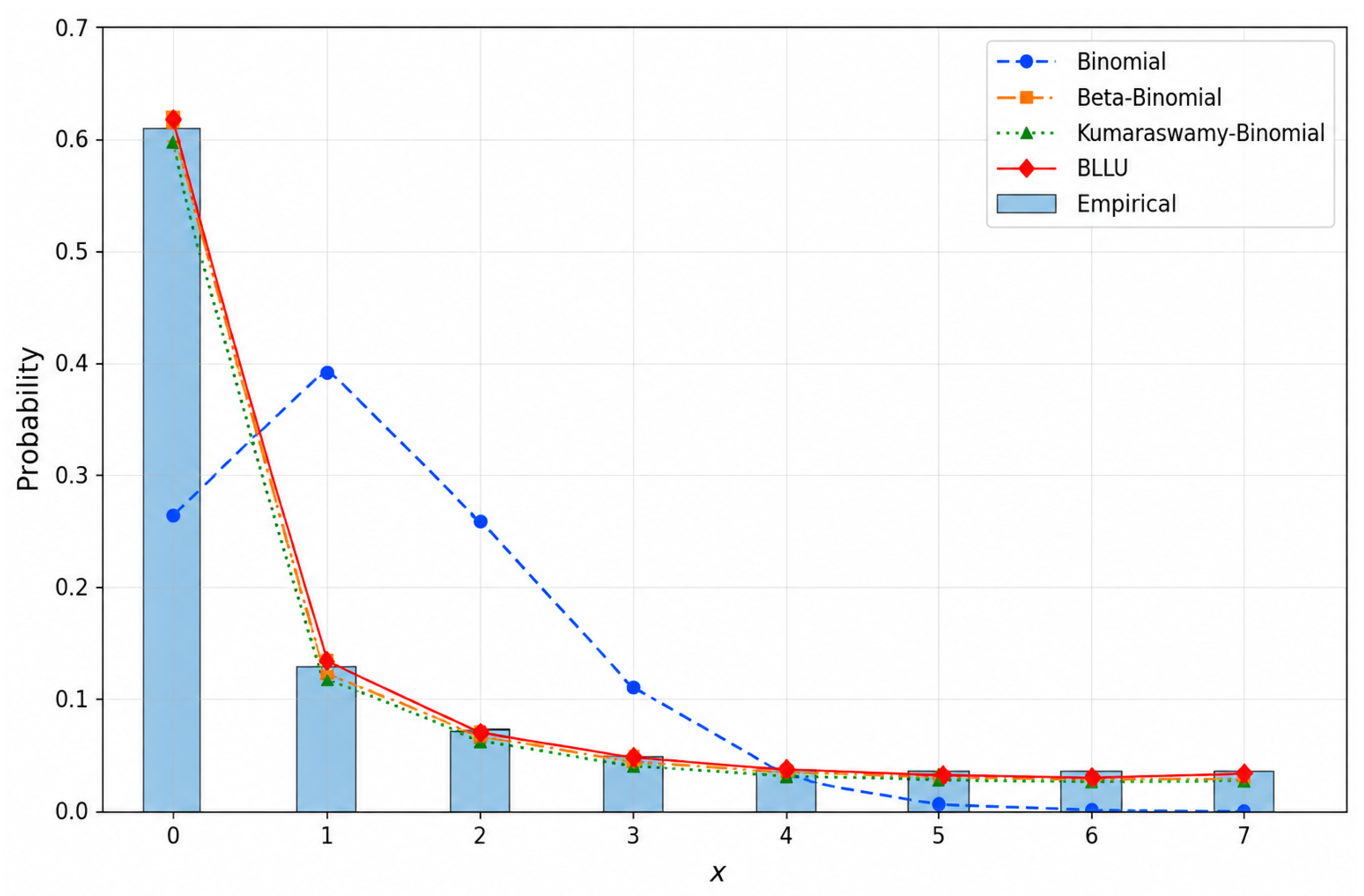
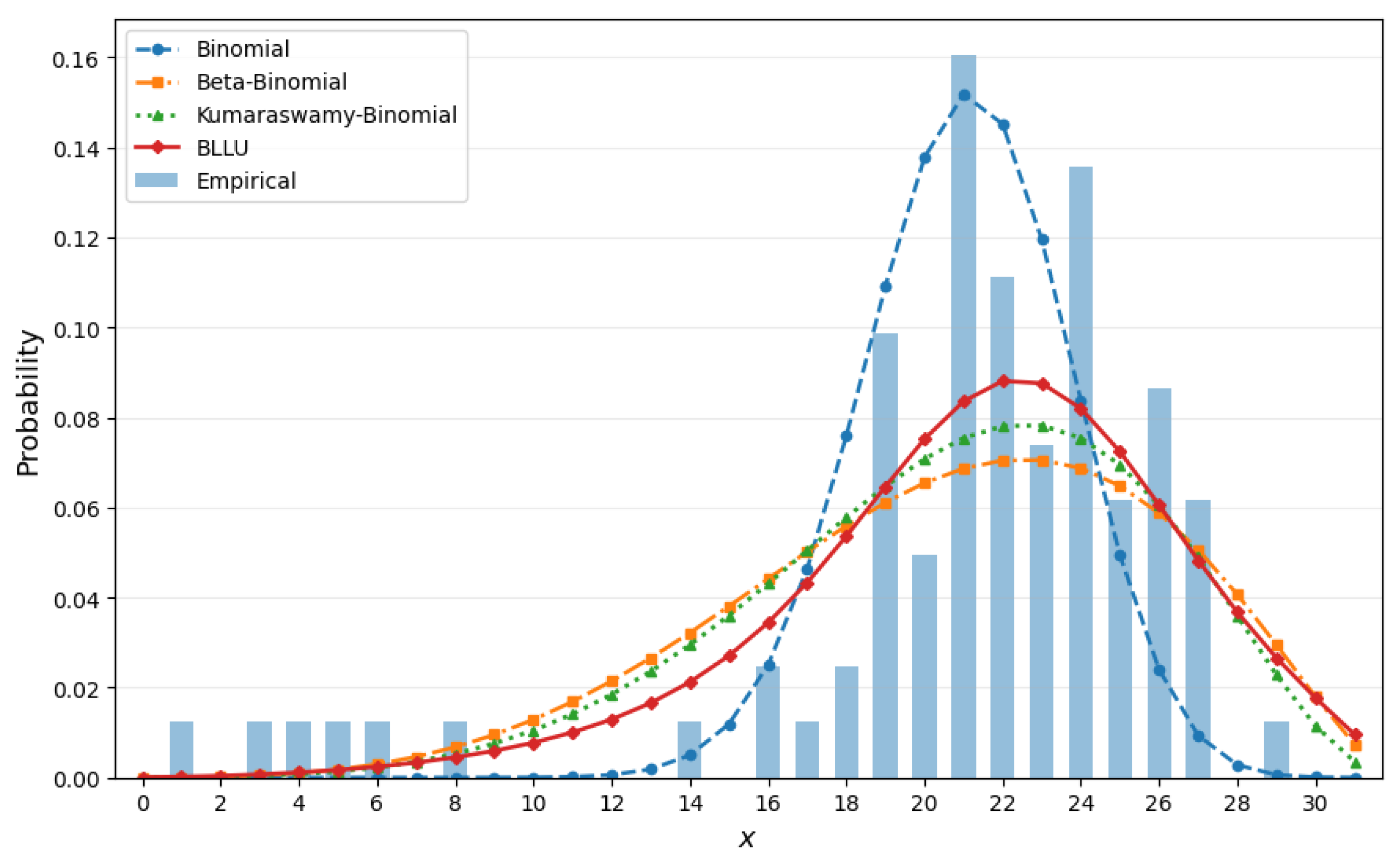
The results thus obtained show a substantial improvement of the three binomial mixture models over the ordinary binomial model. As can be seen, the ordinary binomial model is rejected by both goodness-of-fit tests, and does not represent an adequate model for fitting this empirical distribution. Conversely, for the three mixture models, neither the CVM nor the AD test rejects the null hypothesis at the 5% significance level. In this way, the goodness-of-fit results provide additional evidence that the introduction of mixing substantially improves the description of the observed exceedance counts, as can also be seen in Figure 4, which displays the empirical and fitted probability mass functions. Nevertheless, although the AIC and BIC differences between the three mixture models are modest, the BLLU model reduces the MSE by approximately relative to the beta-binomial model and relative to the Kumaraswamy–binomial model, while also yielding substantially lower CvM and AD statistics. Thus, its favorable performance is reflected not only in the information criteria but also in the direct goodness-of-fit measures.
Figure 4.
Empirical and fitted probability mass functions for the number of days in a seven-day period with SO2 concentration exceeding 20 .
In addition, the empirical dispersion index for this dataset is equal to . According to Equation (17), the fitted BLLU distribution has a theoretical dispersion index of approximately 3.27, closely matching the empirical value. This agreement provides additional support for the adequacy of the BLLU fit, complementing the goodness-of-fit results reported above. Finally, the estimated value indicates positive skewness of the fitted BLLU distribution, in accordance with the asymmetry result established in Section 2. This is also consistent with the pronounced concentration of observations at and the extended right tail of the empirical PMF, shown in Figure 4. It is clear that the ordinary binomial model fails to reproduce the pronounced concentration at and the extended upper tail. In contrast, the three mixture models provide a substantially more flexible description of the empirical distribution, with the BLLU model showing the closest overall agreement and the smallest MSE.
4.2. Application to Road Traffic Accident Data
The second dataset consists of records of traffic accidents in Serbia for the period from 1 January 2015 to 31 July 2026. It is obtained from publicly available open-data records published by the Ministry of Interior of the Republic of Serbia through the Serbian Open Data Portal [32]. Each record contains information on the date and time of the accident, municipality, geographical coordinates, and the severity of its consequences. For the present analysis, we consider the most serious road traffic accidents involving at least one fatality. To construct a bounded count variable suitable for the proposed model, we consider only months with 31 days and define the count variable:
Consequently, and the natural binomial parameter is fixed at . The eleven complete years from 2015 to 2025 yield 77 monthly observations, and additional data available until July 31, 2026 contains four months of 31 days each (January, March, May, and July), giving a total sample size of . The restriction to 31-day months ensures a common binomial support () and yields 81 monthly observations over the period January 2015–July 2026. This provides a consistent basis for illustrating the flexibility of the proposed BLLU distribution in modelling fatal road traffic accident data. Although the selected months do not cover all calendar months, the application offers an additional empirical assessment of the model in a distinct field. An extension based on month-specific values of n could incorporate the entire observation period. The empirical frequency distribution of X is shown in Table 6. The observed values range from 1 to 29, with the highest frequency at , while the sample mean and empirical variance are, respectively, and Hence, the empirical variance exceeds the sample mean indicating clear overdispersion relative to the ordinary binomial model and providing empirical support for the role of mixing heterogeneity captured by the proposed BLLU model.
Table 6.
Empirical frequencies of the number of days with at least one fatal traffic accident in a 31-day month.
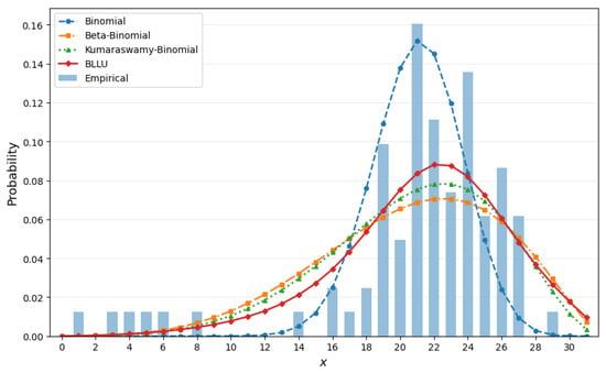
In the following, the same four considered models were fitted to this grouped data, using MLE for all model parameters, including the proposed BLLU framework. The likelihood function for grouped data is given as in Equation (30), with , and the corresponding model probability . The estimated parameters and the resulting fit statistics are reported in the following table, Table 7. Among the four considered models, the BLLU distribution yields the largest log-likelihood and the smallest AIC, BIC, MSE, CVM, and AD values. Moreover, it is the only model for which neither the CVM nor the AD test rejects the null hypothesis at the 5% significance level. In addition, the empirical dispersion index, , indicates overdispersion, with a theoretical dispersion index of approximately 1.11. Although the degree of overdispersion is less pronounced than in empirical data, it still indicates its presence relative to the ordinary binomial model, which prompts the consideration of more flexible mixture distributions. Finally, the estimated value indicates negative skewness of the fitted BLLU distribution, in accordance with the asymmetry result established earlier. This is consistent with the longer lower tail of the empirical distribution, whose mode is at and which extends much farther toward the lower boundary than toward the upper boundary.
Table 7.
Parameter estimates, fit statistics, and goodness-of-fit results for the competing models fitted to the traffic accident data.
Figure 5 displays the empirical and fitted probability mass functions. It is interesting to note that, although the ordinary binomial model captures the dominant central part of the distribution, it assigns very small probability to the lower tail observed in the data. Conversely, the three mixture models provide greater flexibility in describing this part of the distribution, with the BLLU model showing the closest overall agreement with the empirical distribution.
Figure 5.
Empirical and fitted probability mass functions for the number of days with at least one fatal traffic accident in a 31-day month.
5. Conclusions
In this paper, we introduced the binomial Laplace–Logistic Unit (BLLU) distribution, a new two-parameter binomial mixture model obtained by assuming that the success probability follows the Laplace–Logistic Unit (LLU) distribution. We established several probabilistic properties of the proposed distribution, including its probability mass function, factorial and ordinary moments, dispersion, symmetry, skewness, modality, and limiting behaviour. In particular, the mean-square convergence of the normalized BLLU random variable to its underlying LLU mixing variable was proved, providing a theoretical motivation for the proposed large-n quantile-based estimation procedure.
The finite-sample performance of the method of moments, maximum likelihood, and quantile-based estimation procedures was investigated through a Monte Carlo study involving three parameter configurations. The numerical results indicate that estimation accuracy generally improves with increasing sample size, although the relative performance of the procedures depends on the parameter being estimated and the considered configuration. Thus, no single estimation method uniformly outperforms the others in all investigated settings.
The empirical applicability of the BLLU distribution was illustrated using weekly counts of sulfur dioxide concentration exceedances and monthly counts of days with at least one fatal road traffic accident in Serbia. In both applications, the BLLU model provided a favourable fit according to the considered likelihood-based and goodness-of-fit criteria, compared with the three alternative binomial models included in the analysis. These findings support the potential usefulness of the proposed distribution for the examined bounded count data, but do not imply universal superiority over other binomial mixture models or establish its adequacy for other datasets.
A limitation of the proposed model is its finite support, determined by the binomial parameter. Furthermore, the BLLU distribution describes the marginal behaviour of bounded counts and does not explicitly account for temporal dependence or nonstationarity. In practical applications, changes in exposure, environmental conditions, reporting practices, and other time-varying factors may influence the observed counts. Therefore, the empirical results presented here should be interpreted as marginal distributional assessments. Future research may consider extensions incorporating covariates, time-varying parameters, or explicit dependence structures, as well as related mixtures based on unbounded count distributions, such as the negative binomial distribution combined with the LLU or other flexible mixing distributions.
Supplementary Materials
The following supporting information can be downloaded at https://www.mdpi.com/article/10.3390/appliedmath6110199/s1.
Author Contributions
Conceptualization, V.S.S. and D.S.; methodology, V.S.S. and D.S.; software, V.S.S. and M.L.Ć.; validation, V.S.S. and M.L.Ć.; formal analysis, V.S.S. and D.S.; data curation, V.S.S. and D.S.; writing—original draft preparation, V.S.S., D.S. and M.L.Ć.; writing—review and editing, D.S. and M.L.Ć.; visualization, V.S.S. and M.L.Ć.; supervision, V.S.S. and D.S.; project administration, D.S. and M.L.Ć. All authors have read and agreed to the published version of the manuscript.
Funding
This research received no external funding.
Data Availability Statement
The raw data used in this study are provided in the Supplementary Materials. The data were obtained from publicly available datasets provided by the Serbian Environmental Protection Agency (SEPA) and the Ministry of Interior of the Republic of Serbia through the Serbian Open Data Portal.
Conflicts of Interest
The authors declare no conflict of interest.
References
- Crowder, M.J. Beta-Binomial ANOVA for Proportions. Appl. Stat. 1978, 27, 34–37. [Google Scholar] [CrossRef] [Scilit] [PubMed]
- Li, X.; Huang, Y.; Zhao, X. The Kumaraswamy Binomial Distribution. Chin. J. Appl. Probab. Stat. 2011, 27, 511–521. [Google Scholar]
- Irshad, M.R.; Shibu, D.; Maya, R.; D’Cruz, V. Binomial Mixture Lindley Distribution: Properties and Applications. J. Indian Soc. Probab. Stat. 2020, 21, 437–469. [Google Scholar] [CrossRef] [Scilit]
- Chesneau, C.; Bakouch, H.S.; Akdoğan, Y.; Karakaya, K. The Binomial-Discrete Poisson-Lindley Model: Modeling and Applications to Count Regression. Commun. Math. Res. 2022, 38, 28–51. [Google Scholar] [CrossRef] [Scilit]
- Azimi, S.S.; Bahrami Samani, E.; Ganjali, M. Analysis of Mixed Correlated Overdispersed Binomial and Ordinal Longitudinal Responses: LogLindley-Binomial and Ordinal Random Effects Model. J. Appl. Stat. 2022, 49, 1742–1768. [Google Scholar] [CrossRef] [Scilit] [PubMed]
- Reyes, J.; Najera-Zuloaga, J.; Lee, D.-J.; Arrué, J.; Iriarte, Y.A. A Bimodal Extension of the Beta-Binomial Distribution with Applications. Axioms 2024, 13, 662. [Google Scholar] [CrossRef] [Scilit]
- Elshahhat, A.; Abo-Kasem, O.E.; Mohammed, H.S. Statistical Evaluation of Beta-Binomial Probability Law for Removal in Progressive First-Failure Censoring and Its Applications to Three Cancer Cases. Mathematics 2025, 13, 3028. [Google Scholar] [CrossRef] [Scilit]
- Basu, P.; Brill, B.; Yekutieli, D. Exact Confidence Intervals for the Mixing Distribution from Binomial Mixture Distribution Samples. J. Comput. Graph. Stat. 2026, 35, 880–890. [Google Scholar] [CrossRef] [Scilit]
- Zamani, H.; Taghipour, M.; Saber, M.M. Inference on Binomial Log-Lindley Distribution Using Generalized Hybrid Censoring Data with Application to Accident Data. Qual. Quant. 2026, 60, 10445–10471. [Google Scholar] [CrossRef] [Scilit]
- Salinas, H.S.; Bakouch, H.S.; Almuhayfith, F.E.; Caimanque, W.E.; Barrios-Blanco, L.; Albalawi, O. Statistical Advancement of a Flexible Unitary Distribution and Its Applications. Axioms 2024, 13, 397. [Google Scholar] [CrossRef] [Scilit]
- Biçer, C.; Bakouch, H.S.; Biçer, H.D.; Alomair, G.; Hussain, T.; Almohisen, A. Unit Maxwell-Boltzmann Distribution and Its Application to Concentrations Pollutant Data. Axioms 2024, 13, 226. [Google Scholar] [CrossRef] [Scilit]
- Stojanović, V.S.; Jovanović Spasojević, T.; Bojičić, R.; Pažun, B.; Langović, Z. Cauchy–Logistic Unit Distribution: Properties and Application in Modeling Data Extremes. Mathematics 2025, 13, 255. [Google Scholar] [CrossRef] [Scilit]
- Stojanović, V.S.; Bakouch, H.S.; Alomair, G.; Daghestani, A.F.; Grujčić, Ž. A Flexible Unit Distribution Based on a Half-Logistic Map with Applications in Stochastic Data Modeling. Symmetry 2025, 17, 278. [Google Scholar] [CrossRef] [Scilit]
- Genç, M.; Özbilen, Ö. The Unit Inverse Maxwell–Boltzmann Distribution: A Novel Single-Parameter Model for Unit-Interval Data. Axioms 2025, 14, 647. [Google Scholar] [CrossRef] [Scilit]
- Al-Moisheer, A.S.; Sultan, K.S.; Mansour, M.M.M. On Unit J-Shaped Distributions: Properties and Estimation with Applications. Mathematics 2026, 14, 1021. [Google Scholar] [CrossRef] [Scilit]
- Gaete, K.A.; Gómez, Y.M.; Barranco-Chamorro, I.; Segovia, F.A.; Gómez, H.W. The Unit Extended Exponential Distribution: Properties, Inference and Applications. Axioms 2026, 15, 532. [Google Scholar] [CrossRef] [Scilit]
- Afuecheta, E.; Okorie, I.E.; Jallow, H.; Nadarajah, S. A Review of Unit Continuous Probability Distributions. AIMS Math. 2025, 10, 25939–26057. [Google Scholar] [CrossRef] [Scilit]
- Stojanović, V.S.; Jovanović Spasojević, T.; Jovanović, M. Laplace-Logistic Unit Distribution with Application in Dynamic and Regression Analysis. Mathematics 2024, 12, 2282. [Google Scholar] [CrossRef] [Scilit]
- Bagui, S.; Mehra, K.L. The Stirling Numbers of the Second Kind and Their Applications. Ala. J. Math. 2024, 47, 1–22. [Google Scholar]
- van Zwet, W.R. Convex Transformations of Random Variables; Mathematical Centre Tracts 7; Mathematisch Centrum: Amsterdam, The Netherlands, 1964. [Google Scholar]
- Johnson, N.L.; Kotz, S.; Balakrishnan, N. Beta Distributions. In Continuous Univariate Distributions, 2nd ed.; Wiley: New York, NY, USA, 1995; Volume 2. [Google Scholar]
- Dümbgen, L.; Mösching, A. On Stochastic Orders and Total Positivity. ESAIM Probab. Stat. 2023, 27, 461–481. [Google Scholar] [CrossRef] [Scilit]
- Billingsley, P. Probability and Measure, 3rd ed.; Wiley: New York, NY, USA, 1995. [Google Scholar]
- Athreya, K.B.; Lahiri, S.N. Measure Theory and Probability Theory; Springer: New York, NY, USA, 2006. [Google Scholar]
- Martin, V.L.; Tremayne, A.R.; Jung, R.C. Efficient Method of Moments Estimators for Integer Time Series Models. J. Time Ser. Anal. 2014, 35, 491–516. [Google Scholar] [CrossRef] [Scilit]
- Li, B.; Babu, G.J. Asymptotic Theory for Maximum Likelihood Estimation. In Springer Texts in Statistics (STS); Springer: New York, NY, USA, 2019; pp. 237–259. [Google Scholar]
- Nelder, J.A.; Mead, R. A Simplex Algorithm for Function Minimization. Comput. J. 1965, 7, 308–313. [Google Scholar] [CrossRef] [Scilit]
- Gross, J.; Ligges, U. Tests for Normality, R package, version 1.0-4. 2013. Available online: http://CRAN.R-project.org/package=nortest (accessed on 7 September 2026).
- Arnold, T.B.; Emerson, J.W. dgof: Discrete Goodness-of-Fit Tests, R package, version 1.5.1. 2024. Available online: https://CRAN.R-project.org/package=dgof (accessed on 10 September 2026).
- Serbian Environmental Protection Agency. Quality of Air—Verified Daily Data. Serbian Open Data Portal, 2011–2024. Available online: https://data.gov.rs/sr/datasets/kvalitet-vazdukha/ (accessed on 10 September 2026).
- World Health Organization Regional Office for Europe. Air Quality Guidelines: Global Update 2005: Particulate Matter, Ozone, Nitrogen Dioxide and Sulfur Dioxide; WHO Regional Office for Europe: Copenhagen, Denmark, 2006. [Google Scholar]
- Ministry of Interior of the Republic of Serbia. Data on Road Traffic Accidents by Police Departments and Municipalities. Serbian Open Data Portal, 2015–2026. Available online: https://data.gov.rs/sr/datasets/podatsi-o-saobratshajnim-nezgodama-po-politsijskim-upravama-i-opshtinama/ (accessed on 13 September 2026).

Disclaimer/Publisher’s Note: The statements, opinions and data contained in all publications are solely those of the individual author(s) and contributor(s) and not of MDPI and/or the editor(s). MDPI and/or the editor(s) disclaim responsibility for any injury to people or property resulting from any ideas, methods, instructions or products referred to in the content. |
© 2026 by the authors. Licensee MDPI, Basel, Switzerland. This article is an open access article distributed under the terms and conditions of the Creative Commons Attribution (CC BY) license.