A Complete Characterisation of Half-Sunlet Decompositions of Line Graphs of Complete Graphs

Abstract

Let $L\left(K_n\right)$ be the line graph of $K_n$ and let ${\mathrm{HS}}_6$ be the graph obtained from a 4-cycle by attaching a pendant edge at each of two antipodal vertices. We prove that $L\left(K_n\right)$ has an ${\mathrm{HS}}_6$-decomposition if and only if $n\ge 4$ and $n\not\equiv 3(mod4)$. The proof splits $L\left(K_n\right)$ into smaller line graphs together with graphs $W(m,k)$ built from k triangle bundles glued along shared degree-two vertices, characterises the single-copy case, and handles $W(m,2)$ via a construction attached to each cycle of a cycle decomposition of $K_m$.

1. Introduction

All graphs here are finite and simple. For a graph G, we write $V\left(G\right)$ and $E\left(G\right)$ for its vertex and edge sets and $P_2\left(S\right)$ for the set of 2-element subsets of a set S. An edge with ends u and v is written $\{u,v\}$, and a cycle whose consecutive vertices are $v_1,v_2,\dots ,v_r$ (so that its edges are $\{v_1,v_2\},\dots ,\{v_{r-1},v_r\},\{v_r,v_1\}$) is written $(v_1,v_2,\dots ,v_r)$. The subscript of a standard graph always records its number of vertices: $K_n$ is the complete graph on n vertices, $C_k$ the cycle on k vertices (hence with k edges), $P_k$ the path on k vertices (hence with $k-1$ edges), and $K_{a,b}$, $K_{a,b,c}$ the complete bipartite and tripartite graphs with parts of the indicated sizes. The one exception, kept to agree with the literature on star decompositions, is the star $S_k=K_{1,k}$, indexed by its number k of edges. A vertex of degree one is a leaf (or pendant vertex), and the edge incident with it is a pendant edge; we use leaf only for the vertex and pendant edge only for the edge. If $H_1,\dots ,H_r$ are pairwise edge-disjoint subgraphs of G with $E\left(G\right)={\bigcup }_{i}E\left(H_i\right)$, we write $G=H_1\oplus H_2\oplus \cdots \oplus H_r,$ and, if $H_i\cong H$ for every i, we say that H decomposes G and write $H\mid G$. Since the $H_i$ partition $E\left(G\right)$, the divisibility condition

$$\left|E\right(H\left)\right|{\displaystyle |}\left|E\right(G\left)\right|$$

(1)

is necessary for $H\mid G$. The line graph $L\left(G\right)$ has vertex set $E\left(G\right)$, with two vertices being adjacent precisely when the corresponding edges of G meet at a vertex.

Deciding, for a fixed pattern H, which members of a given host family admit an H-decomposition is a central and long-studied problem of design theory. For complete hosts, the basic patterns are well understood: cycles of a fixed length [1] and of arbitrarily prescribed lengths [2] in $K_n$; even cycles in $K_{m,n}$ [3]; stars of varying sizes in complete multigraphs [4]; mixtures of paths, stars, and cycles with four edges apiece [5]; and trees [6]. No general method is to be expected, since the H-decomposition problem is NP-complete for every connected H with at least three edges [7]; each new combination of pattern and host therefore needs its own argument, and the techniques that work depend strongly on the shape of H. The host considered in this paper is one about which far less is known.

Against this background, the line graph of the complete graph is a markedly more challenging host, and progress regarding it has been incremental and pattern-by-pattern. Colby and Rodger [8] treated short cycles in $L\left(K_n\right)$, and Cox [9] determined the full spectrum of 6-cycle systems. The organising question was posed by Cox and Rodger [10], who asked for which m and n the graph $L\left(K_n\right)$ admits an m-cycle decomposition; this problem remains open in general. Uniform patterns other than cycles have also been settled on this host: Xin and Yang [11] recently showed that, for a prime $k>2$ and $n\ge k+1$, $L\left(K_n\right)$ has an $S_k$-decomposition (into stars with k edges) if and only if $n\equiv 0,1,2(modk)$—the same residue pattern as for cycles and paths of prime length, since stars, like cycles and paths, are regular or single-non-leaf-degree patterns. Partial answers have accumulated steadily: Heinrich and Nonay [12] handled exact coverings of 2-paths by 4-cycles, Verrall [13] constructed perfect sets of Euler tours yielding Hamilton decompositions, Ganesamurthy and Paulraja [14] settled the $C_5$ case for the $\lambda$-fold line graph, and Ganesamurthy, Paulraja, and Srimathi [15] turned to multidecompositions, showing that the obvious numerical conditions suffice for a $\{C_3^{\alpha },P_4^{\beta },B^{\gamma }\}$-decomposition of $L\left(K_n\right)$, where B is the bowtie (two triangles sharing a vertex), and characterising $\{C_3^{\alpha },K_{1,3}^{\beta }\}$-decompositions. Their arguments proceed through the intersection graph of a $C_3$-decomposition of $L\left(K_n\right)$, whose existence they establish by an induction ([15], Theorem 3.1) that is, in the notation of Section 5 below, exactly the statement that the triangle bundle $K_n^{*}$ decomposes into its $\left({\displaystyle \genfrac{}{}{0pt}{}{n}{2}}\right)$ private triangles.

The $\lambda$-fold setting has seen parallel recent progress: Zhao, Wei, and Yang [16] characterised $C_4$-decompositions of the $\lambda$-fold line graph of the complete bipartite graph $K_{m,n}$, extending the $\lambda =1$ line of work of Colby and Rodger and the $C_5$ result of Ganesamurthy and Paulraja [14] already mentioned above; we return to this connection in Section 9. Most relevant to the present paper, Ganesamurthy [17] went on to answer the original Cox–Rodger question itself for $m=p$ an odd prime, proving that, for every prime $p\ge 7$, the graph $L\left(K_n\right)$ decomposes into $\alpha$ cycles and $\beta$ paths of length p exactly when the edge count permits, i.e., when

$$p(\alpha +\beta )=n\left({\displaystyle \genfrac{}{}{0pt}{}{n-1}{2}}\right)=\left|E\left(L\left(K_n\right)\right)\right|,$$

deducing from this a complete characterisation of $C_p$-decompositions, together with one of $P_{k+1}$-decompositions when k is a power of an odd prime. The technique of [17], which reduces $L\left(K_n\right)$ to smaller line graphs plus auxiliary building blocks assembled from subdivisions and circulants, is the point of departure for the present paper, and one of its structural observations is recalled as Lemma 1 below.

It is worth recording a folklore expectation, noted in [15] and attributed there to [10]: whenever H decomposes $K_n$, one expects H also to decompose $L\left(K_n\right)$ as soon as the numerical conditions permit. Theorem 1 below is a further instance in which this expectation is borne out, and in a particularly clean form, since the divisibility condition turns out to be sufficient with no exceptions whatsoever.

The pattern graph studied here belongs to the half-sunlet family ${\mathrm{HS}}_{3k}$, introduced and named by Gajendran Palaniyandi, Aramuthakannan Soundararajan, and Sandhya Soundararajan in a companion article [18], published in Mathematics (2026), that shares its full author team with the present paper and determines exactly when the member ${\mathrm{HS}}_{12}$ (the case $k=4$ below, an octagon with pendant edges at four alternating vertices) decomposes the complete graph $K_a$, the complete bipartite graph $K_{a,b}$, and the complete tripartite graph $K_{a,b,c}$. The present paper treats the smallest nontrivial member of this family against the entirely different host $L\left(K_n\right)$, using a disjoint set of techniques (the splitting identity of Section 4 and the triangle bundle machinery of Section 5 and Section 6), and the two papers share no results, proofs, or certificates. For $k\ge 2$, the member ${\mathrm{HS}}_{3k}$ is obtained from an even cycle $C_{2k}$ by attaching a pendant edge at each of k alternating vertices of the cycle, so that $|V\left({\mathrm{HS}}_{3k}\right)|=|E\left({\mathrm{HS}}_{3k}\right)|=3k,\mathrm{with}\mathrm{degree}\mathrm{sequence}{3}^k{2}^k{1}^k$.

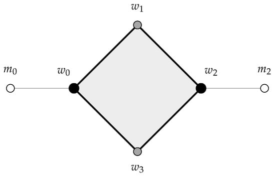
The name records the contrast with the classical sunlet or sun graph $L_{2n}$, in which a pendant edge is attached at every vertex of $C_n$ and the degree sequence is the uniform $3^n{1}^n$; only half of the cycle vertices of ${\mathrm{HS}}_{3k}$ carry a pendant edge. Spectral properties of the sunlet family were studied by Boulet [19] and, more recently, by Rather, Ganie, and Shang [20], but these questions have no bearing on the edge decomposition problem considered here. Our pattern graph is the smallest member, the case $k=2$,

$${\mathrm{HS}}_6=\mathrm{a}4\text{-cycle}\mathrm{with}\mathrm{pendant}\mathrm{edges}\mathrm{at}\mathrm{two}\mathrm{antipodal}\mathrm{vertices},$$

with $|V\left({\mathrm{HS}}_6\right)|=|E\left({\mathrm{HS}}_6\right)|=6$ and degree sequence $(3,3,2,2,1,1)$; see Figure 1.

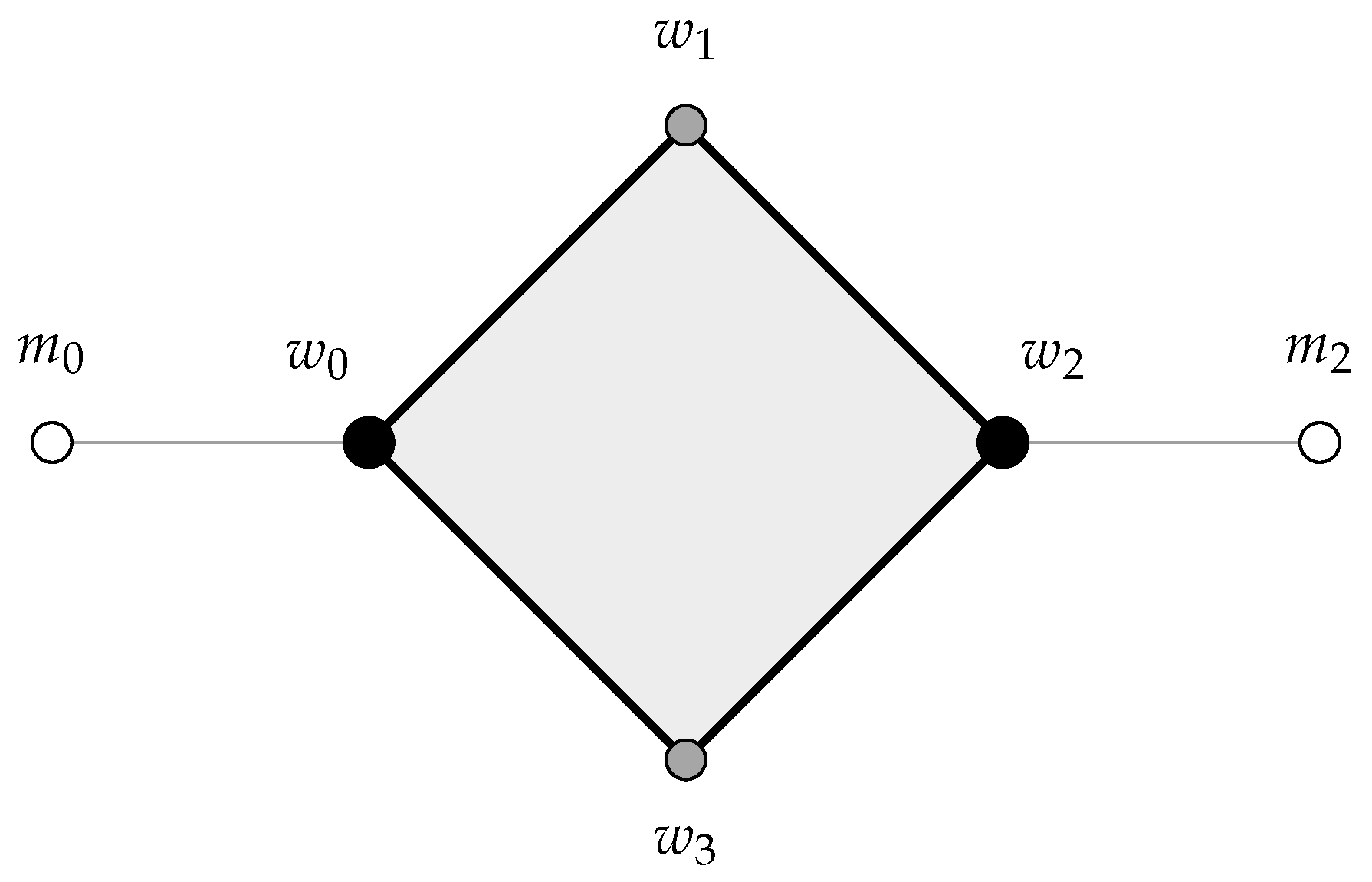
Figure 1. The half-sunlet graph ${\mathrm{HS}}_6$. The shaded quadrilateral is the 4-cycle $(w_0,w_1,w_2,w_3)$ (thick edges); the two grey edges are the pendant edges, attached at the antipodal cycle vertices $w_0$ and $w_2$. The three vertex classes are drawn differently: the hubs $w_0,w_2$ (solid) have degree 3, the remaining cycle vertices $w_1,w_3$ (shaded) degree 2, and the leaves $m_0,m_2$ (hollow) degree 1, giving the mixed degree sequence $(3,3,2,2,1,1)$ and $|V\left({\mathrm{HS}}_6\right)|=|E\left({\mathrm{HS}}_6\right)|=6$. Note that no edge of ${\mathrm{HS}}_6$ joins two vertices of equal degree and that ${\mathrm{HS}}_6$ is bipartite with classes $\{w_0,w_2\}$ and $\{w_1,w_3,m_0,m_2\}$.

1.1. Why ${\mathit{HS}}_{\mathit{6}}$ and Why Existing Techniques Do Not Suffice

There are two reasons for studying ${\mathrm{HS}}_6$ first. It is the smallest member of the half-sunlet family, and it has six edges, like the 6-cycle [9] and the bowtie [15], the two six-edge patterns already settled on $L\left(K_n\right)$, so the answer can be compared directly with theirs (see the discussion after Theorem 1). What separates ${\mathrm{HS}}_6$ from every pattern previously decomposed against $L\left(K_n\right)$ is its degree sequence. Cycles, paths, stars, and bowties are either regular or have all their non-leaf vertices of a single degree, whereas ${\mathrm{HS}}_6$ has two vertices of each of the degrees 3, 2, and 1. This difference defeats each of the three routes by which earlier results on $L\left(K_n\right)$ were obtained.

(a)

The clique route. For each vertex x of $K_n$, the pairs of edges of $K_n$ meeting at x span a clique $Q_x\cong K_{n-1}$ of $L\left(K_n\right)$, and $E\left(L\left(K_n\right)\right)={⨁}_{x}E\left(Q_x\right)$. Hence, any H that decomposes $K_{n-1}$ also decomposes $L\left(K_n\right)$; this is the source of the folklore expectation recalled above. For $H={\mathrm{HS}}_6$, this route requires $6\mid \left({\displaystyle \genfrac{}{}{0pt}{}{n-1}{2}}\right)$—that is, $n\equiv 1,2,5,10(mod12)$. Since the admissible values $n\not\equiv 3(mod4)$ fill the nine classes $n\equiv 0,1,2,4,5,6,8,9,10(mod12)$, the clique route cannot reach the five classes $n\equiv 0,4,6,8,9(mod12)$, whatever is known about ${\mathrm{HS}}_6$-decompositions of complete graphs. For these n, some blocks must use edges from two different cliques $Q_x$ and $Q_y$.

(b)

The trail route. A cycle or a path is a single trail, so decompositions into cycles and paths can be assembled by cutting closed trails (Euler tours, for instance, as in [13]) or circulant difference cycles into consecutive segments and by joining shorter paths end to end; the reductions of [17] for $C_p$ and $P_{k+1}$ rely on such operations. The graph ${\mathrm{HS}}_6$ has four vertices of odd degree ($w_0,w_2,m_0,m_2$), so it is not the edge set of any single trail, and no operation of cutting or joining trails produces it.

(c)

The star route. A decomposition into stars $S_k$ is the same as an orientation of the host in which every out-degree is a multiple of k (each vertex’s out-edges are grouped into stars centred there). The problem is therefore a counting condition at each vertex separately, which is how star results such as those in [11] become tractable. A copy of ${\mathrm{HS}}_6$ has two centres, its hubs, at distance two and joined through a 4-cycle, so no such vertex-by-vertex reduction exists.

The new difficulty appears concretely in the auxiliary graph $K_m^{*}$ produced by our splitting identity. There, the intermediate degree-2 class $\{w_1,w_3\}$ of ${\mathrm{HS}}_6$ forces the shape rigidity phenomenon of Lemma 2: every ${\mathrm{HS}}_6$-decomposition of $K_m^{*}$ is compelled into one structural shape, leaving the decomposer no freedom. This rigidity produces the sharp obstruction $m\equiv 1(mod4)$ of Theorem 3, and its disappearance once copies of $K_m^{*}$ are glued (Remark 3) is the mechanism that the whole construction exploits. A regular or single-non-leaf-degree pattern would not exhibit this behaviour, which is why we regard ${\mathrm{HS}}_6$ as close to the simplest pattern for which the phenomenon can occur at all.

Our main theorem is a complete characterisation, with no exceptional cases.

Theorem 1.

(Main Theorem). For every integer n,

$${\mathrm{HS}}_6\mid L\left(K_n\right)\iff n\ge 4\mathit{and}n\not\equiv 3(mod4).$$

It is striking that the same spectrum was obtained in [15] for a structurally very different pattern of the same size. The bowtie B also has six edges, so setting $\alpha =\beta =0$ in ([15], Theorem 1.1) gives $B\mid L\left(K_n\right)$ precisely when $6\mid \left({\displaystyle \genfrac{}{}{0pt}{}{n}{2}}\right)(n-2)$—that is, again, precisely when $n\not\equiv 3(mod4)$; equivalently, the maximum bowtie packing of $L\left(K_n\right)$ has empty leave for $n\equiv 0,1,2(mod4)$ and leave $K_3$ for $n\equiv 3(mod4)$ ([15], Corollary 1.3). Thus, the two six-edge graphs

$$B(\mathrm{degree}\mathrm{sequence}\text{:}4,2^4),{\mathrm{HS}}_6(\mathrm{degree}\mathrm{sequence}\text{:}{3}^2,2^2,1^2),$$

one with a cut vertex of degree 4 and no vertex of degree 1 and the other with two vertices of each of the degrees $3,2,1$, decompose exactly the same line graphs $L\left(K_n\right)$—although, as the proofs show, for quite different structural reasons.

The necessity in Theorem 1 is the divisibility condition (1) (Proposition 1). The sufficiency rests on three ingredients. First, a splitting identity (Lemma 1) writes $L\left(K_{n_1+n_2}\right)$ as two smaller line graphs together with two graphs $W(m,k)$, each consisting of k copies of a triangle bundle $K_m^{*}$ glued along a common set of degree-two vertices. Second, the single-copy case is settled exactly: ${\mathrm{HS}}_6\mid K_m^{*}$ if and only if $m\equiv 1(mod4)$ (Theorem 3). This negative half is what forces attention onto $k\ge 2$, where the shared vertices acquire degree $2k\ge 4$ and the obstruction vanishes (Remark 3). Third, and the combinatorial heart of the paper, an explicit block family attached to any cycle of $K_m$ (Lemma 3) combines with Veblen’s theorem to give ${\mathrm{HS}}_6\mid W(m,2)$ for every $m\ge 3$ (Lemma 4).

1.2. Novelty of the Present Work

To the best of our knowledge, no H-decomposition of $L\left(K_n\right)$ has previously been determined for any member H of the half-sunlet family, so none of the results below is a specialisation of an existing statement. We summarise what is new.

(i)

A new host for the half-sunlet family. Decomposition results for ${\mathrm{HS}}_{3k}$ have so far concerned the complete and complete multipartite hosts [18]. Theorem 1 is the first such result for line graphs, and it is exception-free: the divisibility condition $n\not\equiv 3(mod4)$ is not merely necessary but sufficient, with no sporadic families excluded.

(ii)

A new pattern for the line graph host. Work on $L\left(K_n\right)$ has concentrated on cycles, paths, and, most recently, stars [8,9,10,11,17] and on multidecompositions into them [15]. The half-sunlet is the first pattern of mixed degree sequence to be treated on this host; Section 1.1 explains why the clique, trail, and star routes used for the earlier patterns do not apply to it.

(iii)

The graphs $W(m,k)$ and a gluing phenomenon. Definition 3 isolates the family obtained by gluing k triangle bundles along a shared set of degree-two vertices, and Theorem 3 together with Remark 3 exhibits a sharp contrast: $K_m^{*}=W(m,1)$ is decomposable only for $m\equiv 1(mod4)$, yet the obstruction disappears entirely once $k\ge 2$, because the shared vertices pass from degree 2 to degree $2k$. We are not aware of a comparable phenomenon in the decomposition literature, and it is what makes the whole induction possible.

(iv)

The cycle unit. Lemma 3 attaches an explicit r-block decomposition to any cycle of length $r\ge 3$ in $K_m$, converting an arbitrary cycle decomposition of $K_m$ into an ${\mathrm{HS}}_6$-decomposition of $W(m,2)$. Combined with Veblen’s theorem, this handles all odd m at a stroke, with two small certificates absorbing the parity defect for even m (Lemma 4). The construction is uniform in r and requires no case analysis.

(v)

Explicit and verifiable output. Every step is constructive. The proof of Theorem 1 unwinds to an explicit block list for each admissible n, and the whole argument rests on only five finite certificates, all given in Section 8.

2. Preliminaries

Definition 1.

(The graph ${\mathrm{HS}}_6$). ${\mathrm{HS}}_6$ consists of the 4-cycle $(w_0,w_1,w_2,w_3)$, with edges $\{w_0,w_1\}$, $\{w_1,w_2\}$, $\{w_2,w_3\}$, $\{w_3,w_0\}$, together with the two pendant edges $\{w_0,m_0\}$ and $\{w_2,m_2\}$ at the antipodal vertices $w_0,w_2$, where $m_0\ne m_2$ are two further vertices (Figure 1). We call $w_0,w_2$ the hubs and $m_0,m_2$ the leaves. A copy of ${\mathrm{HS}}_6$ is recorded as the array

$$\left(\begin{array}{ccccc}& m_0& & m_2& \\ w_0& w_1& w_2& w_3& w_0\end{array}\right),$$

whose bottom row traces the 4-cycle with the first and last entries coinciding and whose top row places each leaf in the column immediately following its hub: $w_0$ in column 1, $m_0$ in column 2, $w_2$ in column 3, and $m_2$ in column 4, with the remaining top-row columns being blank. All blocks below follow this convention.

Definition 2.

(Triangle bundle graph). For $m\ge 2$, let $K_m^{*}$ have vertex set $V\left(K_m\right)\cup \{s_{a{a}^{\prime }}:\{a,a^{\prime }\}\in P_2\left(V\left(K_m\right)\right)\}$ and edge set

$$E\left(K_m^{*}\right)=E\left(K_m\right)\cup \left\{\{a,s_{a{a}^{\prime }}\},\{a^{\prime },s_{a{a}^{\prime }}\}:\{a,a^{\prime }\}\in P_2\left(V\left(K_m\right)\right)\right\}.$$

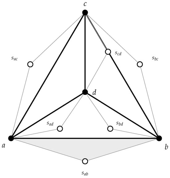
Equivalently, $K_m^{*}$ is obtained from $K_m$ by adding, for every edge $\{x,y\}$, one new vertex joined to x and to y; in the notation of [17], $K_m^{*}=K_m\oplus S_1\left(K_m\right)$, where $S_1$ denotes the subdivision of every edge once. Each edge $\{a,a^{\prime }\}$ of $K_m$ thus lies in a private triangle $\{a,a^{\prime },s_{a{a}^{\prime }}\}$, so each subdivision vertex has no neighbours outside its own triangle and the subdivision vertices form an independent set of size $\left({\displaystyle \genfrac{}{}{0pt}{}{m}{2}}\right)$; see Figure 2. We call $V\left(K_m\right)$ the clique vertices and the $s_{a{a}^{\prime }}$ the subdivision vertices, and we note that

$$\mathrm{deg}\left(s_{a{a}^{\prime }}\right)=2,\mathrm{deg}\left(a\right)=2(m-1),\left|E\left(K_m^{*}\right)\right|=3\left({\displaystyle \genfrac{}{}{0pt}{}{m}{2}}\right).$$

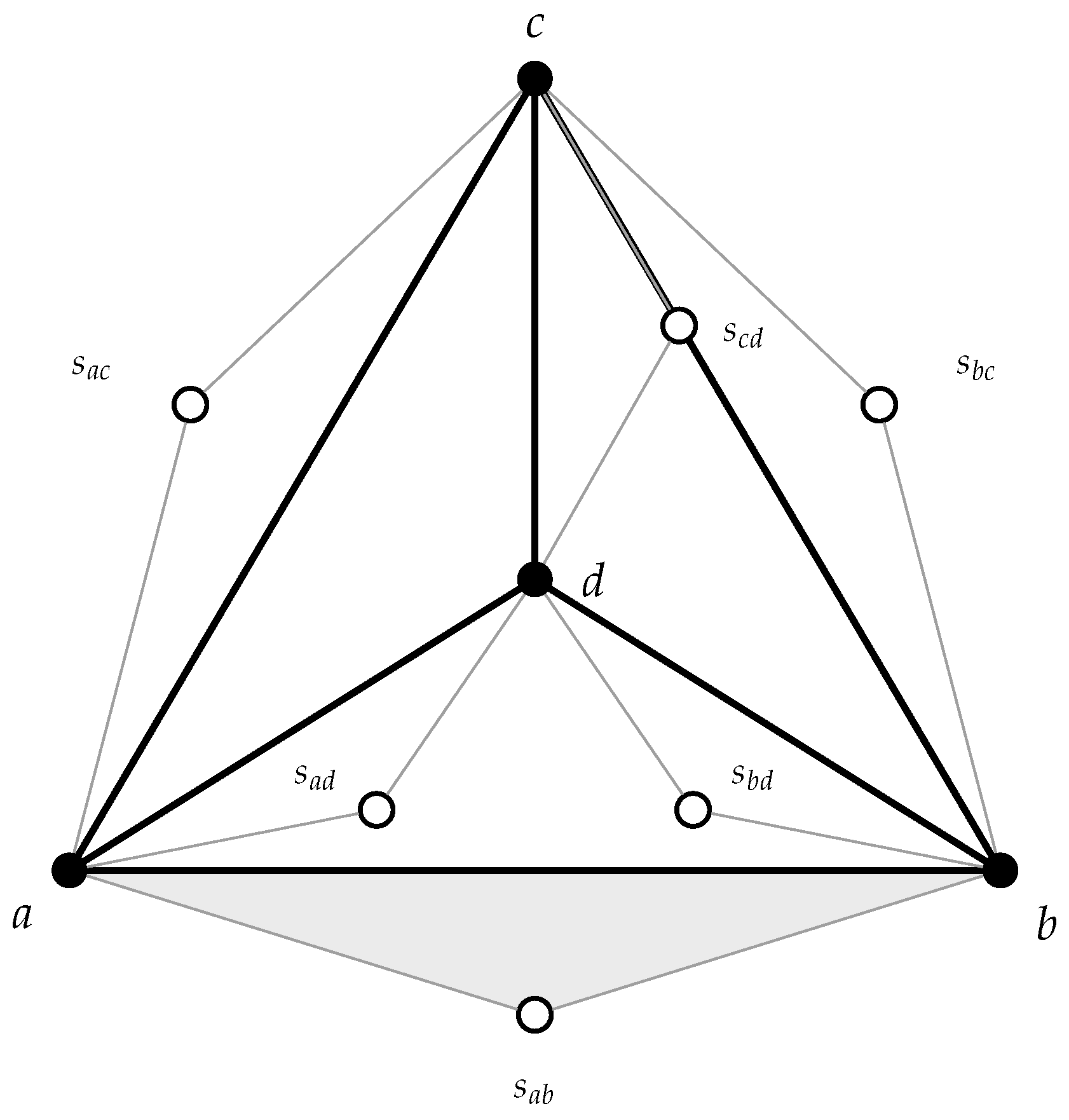
Figure 2. The triangle bundle graph $K_4^{*}=K_4\oplus S_1\left(K_4\right)$, drawn planar so that no edges cross. Solid vertices are the four clique vertices $V\left(K_4\right)=\{a,b,c,d\}$, and thick lines are the six clique edges; hollow vertices are the six subdivision vertices, and thin grey lines are the twelve subdivision edges. Each subdivision vertex $s_{xy}$ is joined to exactly the two ends of its own edge $\{x,y\}$, so every clique edge lies in a private triangle $\{x,y,s_{xy}\}$, meeting the rest of the graph only in x and y; one such triangle, $\{a,b,s_{ab}\}$, is shaded. Thus, $\mathrm{deg}\left(s_{xy}\right)=2$ and $\mathrm{deg}\left(x\right)=2(m-1)=6$ and $|E\left(K_4^{*}\right)|=3\left({\displaystyle \genfrac{}{}{0pt}{}{4}{2}}\right)=18$. The degree-two subdivision vertices can never be hubs of an embedded ${\mathrm{HS}}_6$, which is the source of the rigidity in Lemma 2; gluing $k\ge 2$ such bundles along a shared set of subdivision vertices raises their degree to $2k$ and removes the restriction (Definition 3 and Remark 3).

Definition 3.

(The glued family $W(m,k)$). Let $A,B$ be disjoint with $\left|A\right|=m\ge 2$, $\left|B\right|=k\ge 1$. The graph $W(m,k)$ has vertex set

$$V\left(W(m,k)\right)=\{(a,b):a\in A,b\in B\}\cup \{s_{a{a}^{\prime }}:\{a,a^{\prime }\}\in P_2\left(A\right)\},$$

and, for every $b\in B$ and every $\{a,a^{\prime }\}\in P_2\left(A\right)$, the three edges

$$\{(a,b),(a^{\prime },b)\},\{(a,b),s_{a{a}^{\prime }}\},\{(a^{\prime },b),s_{a{a}^{\prime }}\}.$$

For each fixed b, the subgraph induced by $\{(a,b):a\in A\}\cup \left\{s_{a{a}^{\prime }}\right\}$ is a copy of $K_m^{*}$; these k copies are edge-disjoint and share all subdivision vertices. Hence, $W(m,1)\cong K_m^{*}$ and

$$\left|E\left(W(m,k)\right)\right|=3k\left({\displaystyle \genfrac{}{}{0pt}{}{m}{2}}\right),\mathrm{deg}\left((a,b)\right)=2(m-1),\mathrm{deg}\left(s_{a{a}^{\prime }}\right)=2k.$$

(We use $W(m,k)$ for this family throughout; it is unrelated to the wheel graph, occasionally denoted by $W_n$ elsewhere in the graph decomposition literature.) For $\{a,a^{\prime }\}\in P_2\left(A\right)$, we write $\Gamma (a,a^{\prime })$ for the $3k$ edges just listed and call it the pair gadget of $\{a,a^{\prime }\}$; the pair gadgets partition $E\left(W\right(m,k\left)\right)$. For a subgraph $F\subseteq K_m$ on the vertex set A, we put $\Gamma \left(F\right)={⨁}_{\{a,a^{\prime }\}\in E\left(F\right)}\Gamma (a,a^{\prime })$.

3. The Necessary Condition

Proposition 1.

If ${\mathrm{HS}}_6\mid L\left(K_n\right)$, then $n\ge 4$ and $n\not\equiv 3(mod4)$.

Proof. 

The line graph has $\left({\displaystyle \genfrac{}{}{0pt}{}{n}{2}}\right)$ vertices and

$$|E\left(L\left(K_n\right)\right)|=\sum _{v\in V\left(K_n\right)}\left({\displaystyle \genfrac{}{}{0pt}{}{\mathrm{deg}v}{2}}\right)=n\left({\displaystyle \genfrac{}{}{0pt}{}{n-1}{2}}\right)=\frac{1}{2}n(n-1)(n-2)$$

edges, with each vertex v of $K_n$ contributing the pairs of edges meeting at v. Since $\left|V\right({\mathrm{HS}}_6\left)\right|=6$, an embedding needs $\left({\displaystyle \genfrac{}{}{0pt}{}{n}{2}}\right)\ge 6$, i.e., $n\ge 4$. By (1) with $\left|E\right({\mathrm{HS}}_6\left)\right|=6$,

$$6|\frac{1}{2}n(n-1)(n-2)⟺12\mid n(n-1)(n-2).$$

One of three consecutive integers is a multiple of 3, so $3\mid n(n-1)(n-2)$ always, and the condition reduces to $4\mid n(n-1)(n-2)$. If $n\equiv 0,1,2(mod4)$, then, respectively, n, $n-1$, $n-2$ is divisible by 4. If $n\equiv 3(mod4)$, then n and $n-2$ are odd, while $n-1\equiv 2(mod4)$ supplies only a single factor 2, so $4\nmid n(n-1)(n-2)$. Hence, the condition is exactly $n\not\equiv 3(mod4)$.    □

4. The Splitting Identity

Lemma 1.

Let $n=n_1+n_2$ with $n_1,n_2\ge 1$. Then,

$$L\left(K_n\right)=L\left(K_{n_1}\right)\oplus L\left(K_{n_2}\right)\oplus W(n_1,n_2)\oplus W(n_2,n_1).$$

Proof. 

Partition $V\left(K_n\right)=A\bigsqcup B$ with $\left|A\right|=n_1$, $\left|B\right|=n_2$, so that

$$V\left(L\left(K_n\right)\right)=E\left(K_n\right)=P_2\left(A\right)\bigsqcup P_2\left(B\right)\bigsqcup (A\times B).$$

For $a\in A$ and $b\in B$, we write $(a,b)$ for the vertex of $L\left(K_n\right)$ corresponding to the edge $\{a,b\}$ of $K_n$, and we keep writing $\{a,a^{\prime }\}$ for the vertex corresponding to an edge with both ends in A. Two vertices of $L\left(K_n\right)$ are adjacent exactly when the corresponding edges of $K_n$ share an endpoint, and we sort the adjacent pairs by type.

If both lie in $P_2\left(A\right)$, they are adjacent precisely as in $L\left(K_{n_1}\right)$, and symmetrically for $P_2\left(B\right)$. A pair with one edge in $P_2\left(A\right)$ and the other in $P_2\left(B\right)$ is never adjacent, since these edges are disjoint. Two vertices $(a,b),(a^{\prime },b^{\prime })\in A\times B$ are adjacent iff $a=a^{\prime }$ or $b=b^{\prime }$. Finally, $\{a,a^{\prime }\}\in P_2\left(A\right)$ is adjacent to $(a^{\prime \prime },b)\in A\times B$ iff $a^{\prime \prime }\in \{a,a^{\prime }\}$—that is, $\{a,a^{\prime }\}$ is adjacent to exactly the two vertices $(a,b)$ and $(a^{\prime },b)$ for each $b\in B$.

Fix $b\in B$ and collect the adjacencies just described that involve b. The edges $\{(a,b),(a^{\prime },b)\}$ form a clique on $\{(a,b):a\in A\}\cong K_{n_1}$, and each $\{a,a^{\prime }\}\in P_2\left(A\right)$ is joined to exactly $(a,b)$ and $(a^{\prime },b)$. Under the identification $\{a,a^{\prime }\}\leftrightarrow s_{a{a}^{\prime }}$, this is exactly the b-th copy of $K_{n_1}^{*}$ inside $W(n_1,n_2)$ as in Definition 3; letting b range over B produces all of $W(n_1,n_2)$, the copies sharing $P_2\left(A\right)$. Exchanging the roles of A and B gives $W(n_2,n_1)$, indexed by $a\in A$. Every adjacent pair has been accounted for exactly once.    □

Remark 1.

Lemma 1 is the structural observation used by Ganesamurthy ([17], Observation 2.2); the proof is included to fix the notation of Definition 3. Taking $n_2=1$ recovers the one-vertex form

$$L\left(K_{n+1}\right)=L\left(K_n\right)\oplus K_n^{*},$$

since $W(n,1)\cong K_n^{*}$ while $W(1,n)$ has no edges. An edge count confirms the identity; for instance, with $n_1=n_2=3$,

$$|E\left(L\left(K_6\right)\right)|=60=\underset{L\left(K_3\right)\mathit{twice}}{\underbrace{3+3}}+\underset{W(3,3)}{\underbrace{3·3·3}}+\underset{W(3,3)}{\underbrace{3·3·3}}.$$

5. Decomposing the Triangle Bundle

5.1. An Explicit Construction for $m\equiv 1(mod4)$

Label $V\left(K_m\right)={\mathbb{Z}}_m$ and, for $1\le d\le M:=\frac{m-1}{2}$, let

$$D_d=\left\{\{i,i+d\}:i\in {\mathbb{Z}}_m\right\}$$

be the distance-d class, of size exactly m for odd m; the classes $D_1,\dots ,D_M$ partition $E\left(K_m\right)$. If $m\equiv 1(mod4)$, then M is even, and we set $k=M/2$.

Theorem 2.

Let $m\equiv 1(mod4)$, and, for $1\le j\le k$, put $d_j=j$ and $d_j^{\prime }=M+1-j$. Then, the $\frac{1}{2}\left({\displaystyle \genfrac{}{}{0pt}{}{m}{2}}\right)$ blocks

$$B_{i,j}=\left(\begin{array}{ccccc}& s_{\{w_0,w_0+2j\}}& & s_{\{w_2,w_2-2j\}}& \\ w_0& s_{\{w_0,w_2\}}& w_2& i& w_0\end{array}\right),w_0=i+d_j,w_2=i+d_j^{\prime },$$

for $1\le j\le k$ and $i\in {\mathbb{Z}}_m$, form an ${\mathrm{HS}}_6$-decomposition of $K_m^{*}$.

Proof. 

Each block is a copy of ${\mathrm{HS}}_6$. The vertex $s_{\{w_0,w_2\}}$ is adjacent to exactly $w_0$ and $w_2$, so the edges $\{w_0,s_{\{w_0,w_2\}}\}$ and $\{s_{\{w_0,w_2\}},w_2\}$ exist; the edges $\{w_2,i\}$ and $\{i,w_0\}$ are the clique edges of distances $d_j^{\prime }$ and $d_j$. Since $1\le 2j\le M<\frac{m}{2}$, we have $w_0\ne w_0+2j$ and $w_2\ne w_2-2j$, so both pendant edges exist. Moreover, $d_j\ne d_j^{\prime }$, since $d_j=d_j^{\prime }$ would give $2j=M+1$ with $M+1$ odd; hence, $w_0,w_2,i$ are distinct clique vertices, and $s_{\{w_0,w_2\}}$ is of the subdivision type, so the four cycle vertices are distinct. The degrees within the block are $\mathrm{deg}{w}_0=\mathrm{deg}{w}_2=3$, $\mathrm{deg}{s}_{\{w_0,w_2\}}=\mathrm{deg}i=2$ , and the degree is 1 at each leaf.

Clique edges. For fixed j, as i runs over ${\mathbb{Z}}_m$, the pairs $\{i,i+d_j\}$ and $\{i,i+d_j^{\prime }\}$ run bijectively over $D_{d_j}$ and $D_{d_j^{\prime }}$. Since

$$\{1,2,\dots ,M\}={\displaystyle \underset{j=1}{\overset{k}{⨆}}}\{d_j,d_j^{\prime }\},$$

every clique edge occurs exactly once, either as $\{i,w_0\}$ or as $\{w_2,i\}$, and never both.

Subdivision vertices in cycle position. For fixed j, the outer pair $\{w_0,w_2\}$ has difference $d_j^{\prime }-d_j=M+1-2j$, and, since $0<M+1-2j\le M-1<\frac{m}{2}$, its distance class is $e_j=M+1-2j$; the map $i\mapsto \{w_0,w_2\}$ is a bijection onto $D_{e_j}$. As j runs over $1,\dots ,k$,

$$e_j=M-1,M-3,\dots ,1,$$

the k distinct odd values in $\{1,\dots ,M-1\}$ (M being even). Thus, the subdivision vertices occupying the position $w_1$ are exactly those on odd-distance pairs, each used once.

Pendant edges. Consequently, the even-distance classes $D_2,D_4,\dots ,D_M$ are untouched in cycle position. Fix a clique vertex a and an even distance $2j$ with $1\le j\le k$. Then, a plays the role $w_0$ for index j exactly when $i=a-d_j$, consuming the edge $\{a,s_{\{a,a+2j\}}\}$, and the role $w_2$ exactly when $i=a-d_j^{\prime }$, consuming $\{a,s_{\{a,a-2j\}}\}$. Letting j run over $1,\dots ,k$, the vertex a uses each of its $2k=M$ edges to even-distance subdivision vertices exactly once.

Distinct leaves. If $m_0=m_2$, then $\{w_0,w_0+2j\}=\{w_2,w_2-2j\}$, and, since $w_0\ne w_2$, this forces $w_2-w_0=2j$; however, $w_2-w_0=d_j^{\prime }-d_j=M+1-2j$, giving $M+1\equiv 0(modm)$, which is impossible as $1\le M+1\le m-1$.

Every one of the $3\left({\displaystyle \genfrac{}{}{0pt}{}{m}{2}}\right)$ edges is therefore covered exactly once by $\frac{1}{2}\left({\displaystyle \genfrac{}{}{0pt}{}{m}{2}}\right)$ valid blocks.    □

Example 1.

($m=5$). Here, $M=2$, $k=1$, and the single pair is $(d_1,d_1^{\prime })=(1,2)$, so $e_1=1$: the distance-1 subdivision vertices occupy cycle positions and the distance-2 ones supply the pendant edges. The five blocks $B_{i,1}$, $i\in {\mathbb{Z}}_5$, are

$$\left(\begin{array}{ccccc}& s_{13}& & s_{02}& \\ 1& s_{12}& 2& 0& 1\end{array}\right),\left(\begin{array}{ccccc}& s_{24}& & s_{13}& \\ 2& s_{23}& 3& 1& 2\end{array}\right),\left(\begin{array}{ccccc}& s_{03}& & s_{24}& \\ 3& s_{34}& 4& 2& 3\end{array}\right),$$

$$\left(\begin{array}{ccccc}& s_{14}& & s_{03}& \\ 4& s_{04}& 0& 3& 4\end{array}\right),\left(\begin{array}{ccccc}& s_{02}& & s_{14}& \\ 0& s_{01}& 1& 4& 0\end{array}\right).$$

The ten clique edges appear once each; the five vertices $s_{01},s_{12},s_{23},s_{34},s_{04}$ appear once each in cycle position, contributing 10 edges; and each of $s_{02},s_{13},s_{24},s_{03},s_{14}$ supplies its two edges as pendant edges in two different blocks, contributing the last 10. In total, there are $30=3\left({\displaystyle \genfrac{}{}{0pt}{}{5}{2}}\right)$ edges in 5 blocks.

Remark 2.

By contrast with Theorem 2, the triangle bundle is trivially decomposable into triangles: its $\left({\displaystyle \genfrac{}{}{0pt}{}{m}{2}}\right)$ private triangles $\{a,a^{\prime },s_{a{a}^{\prime }}\}$ are pairwise edge-disjoint and exhaust $E\left(K_m^{*}\right)$. Combined with the case $n_2=1$ of Lemma 1, this yields at once the $C_3$-decomposition of $L\left(K_n\right)$ recorded as ([15], Theorem 3.1), whose inductive step adds precisely the triangles $\left(\right\{i,j\},\{i,n+1\},\{j,n+1\left\}\right)$—that is, the private triangles of $K_n^{*}$. The contrast is instructive: the same graph $K_m^{*}$ that splits effortlessly into triangles admits an ${\mathrm{HS}}_6$-decomposition only for $m\equiv 1(mod4)$, by Theorem 3 below, the difference being that a triangle may use a degree-two subdivision vertex as one of its three equal-degree vertices, whereas ${\mathrm{HS}}_6$ cannot.

5.2. Necessity and Why Gluing Changes the Problem

Lemma 2.

(Shape rigidity). In any ${\mathrm{HS}}_6$-decomposition of $K_m^{*}$, every block has its non-hub cycle vertex $w_1$ equal to a subdivision vertex, and both leaves are subdivision vertices.

Proof. 

A subdivision vertex has degree 2 in $K_m^{*}$ and hence can never be a hub. The unique subdivision vertex adjacent to both $w_0$ and $w_2$ is $s_{\{w_0,w_2\}}$, so $w_1$ and $w_3$ cannot both be subdivision vertices. Every block is therefore either a cherry, with $w_1=s_{\{w_0,w_2\}}$ and $w_3$ a clique vertex, contributing the two clique edges $\{w_2,w_3\}$ and $\{w_3,w_0\}$, or a pure $C_4$, with all of $w_0,w_1,w_2,w_3$ clique vertices, contributing four clique edges. Let $c_1,c_2$ count the two shapes and let p count the pendant edges whose leaf is a clique vertex. Counting blocks and clique edges, respectively,

$$c_1+c_2=\frac{1}{2}\left({\displaystyle \genfrac{}{}{0pt}{}{m}{2}}\right),2c_1+4c_2+p=\left({\displaystyle \genfrac{}{}{0pt}{}{m}{2}}\right).$$

Subtracting twice the first identity from the second yields $2c_2+p=0$, whence $c_2=p=0$.    □

Theorem 3.

${\mathrm{HS}}_6\mid K_m^{*}$ if and only if $m\equiv 1(mod4)$.

Proof. 

Sufficiency is Theorem 2. Conversely, fix a decomposition; by Lemma 2, every block is a cherry with subdivision leaves. Call $\{w_0,w_2\}$ the outer pair of a block. Distinct blocks have distinct outer pairs, since the outer pair determines $w_1=s_{\{w_0,w_2\}}$ and each subdivision vertex occupies a cycle position at most once. Let P be the set of outer pairs, so $\left|P\right|=\frac{1}{2}\left({\displaystyle \genfrac{}{}{0pt}{}{m}{2}}\right)$, and let ${\mathrm{deg}}_P\left(v\right)$ count the members of P containing v.

A clique vertex v is a hub in exactly ${\mathrm{deg}}_P\left(v\right)$ blocks, each demanding one pendant edge at v. Such a pendant edge is an edge $\{v,s_{\{v,x\}}\}$ with $\{v,x\}\notin P$, because a pair in P has its subdivision vertex fully consumed in cycle position. Conversely, if $\{v,x\}\notin P$, then $s_{\{v,x\}}$ lies in no cycle, so both of its edges must serve as pendant edges, and $\{v,s_{\{v,x\}}\}$ can only be a pendant edge at v. Supply therefore equals demand:

$$(m-1)-{\mathrm{deg}}_P\left(v\right)={\mathrm{deg}}_P\left(v\right)⟹{\mathrm{deg}}_P\left(v\right)={\displaystyle \frac{m-1}{2}}\mathrm{for}\mathrm{every}v,$$

which forces m to be odd. Moreover, $\left|P\right|=\frac{1}{2}\left({\displaystyle \genfrac{}{}{0pt}{}{m}{2}}\right)$ must be an integer, so $\left({\displaystyle \genfrac{}{}{0pt}{}{m}{2}}\right)$ is even, i.e., $m\equiv 0,1(mod4)$. Together with m odd, this gives $m\equiv 1(mod4)$.    □

Remark 3.

Lemma 2 depends on subdivision vertices having degree 2 and so never being hubs. In $W(m,k)$, a subdivision vertex has degree $2k$, so, as soon as $k\ge 2$, it may serve as a hub; the rigidity argument collapses, and with it the obstruction of Theorem 3. This is exactly why the glued graphs, not $K_m^{*}$ itself, are the appropriate vehicle; for example, $K_4^{*}=W(4,1)$ admits no ${\mathrm{HS}}_6$-decomposition, whereas $W(4,k)$ does for every $k\ge 2$ (Lemma 5).

6. Cycle Units and the Graphs W (m,2)

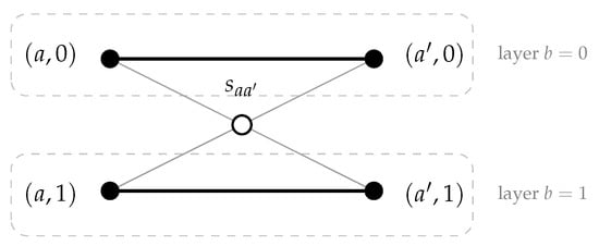
Throughout this section, $k=2$, so $B=\{0,1\}$, and each pair gadget carries the six edges

$$\begin{array}{cc}\hfill \Gamma (a,a^{\prime })=\{& \{(a,0),(a^{\prime },0)\},\{(a,1),(a^{\prime },1)\},\hfill \\ & \{(a,0),s_{a{a}^{\prime }}\},\{(a^{\prime },0),s_{a{a}^{\prime }}\},\{(a,1),s_{a{a}^{\prime }}\},\{(a^{\prime },1),s_{a{a}^{\prime }}\}\};\hfill \end{array}$$

see Figure 3. Since the pair gadgets partition $E\left(W\right(m,2\left)\right)$, any decomposition of $K_m$ into subgraphs $F_1,\dots ,F_r$ induces one of $W(m,2)$:

$$K_m=F_1\oplus \cdots \oplus F_r⟹W(m,2)=\Gamma \left(F_1\right)\oplus \cdots \oplus \Gamma \left(F_r\right),$$

so it suffices to decompose each $\Gamma \left(F_i\right)$.

Figure 3. The pair gadget $\Gamma (a,a^{\prime })$ inside $W(m,2)$, carrying six edges in all. The two thick horizontal edges are the clique edges $\{(a,0),(a^{\prime },0)\}$ and $\{(a,1),(a^{\prime },1)\}$, one in each layer; the four thin grey edges join the single shared subdivision vertex $s_{a{a}^{\prime }}$ to both ends of the pair in both layers. Hence, $\mathrm{deg}\left(s_{a{a}^{\prime }}\right)=2k=4$ here, in contrast with $\mathrm{deg}\left(s_{a{a}^{\prime }}\right)=2$ in a lone triangle bundle (Figure 2); this is precisely the extra degree that allows $s_{a{a}^{\prime }}$ to act as a hub. Since $|E(\Gamma (a,a^{\prime }))|=6=|E\left({\mathrm{HS}}_6\right)|$ and the pair gadgets partition $E\left(W\right(m,2\left)\right)$, decomposing $W(m,2)$ amounts to grouping pair gadgets into families that can be split into blocks.

Lemma 3.

(Cycle unit). Let $C=(a_1,a_2,\dots ,a_r)$ with $r\ge 3$ be a cycle in $K_m$, indices read modulo r, and write $s_i:=s_{a_i{a}_{i+1}}$. Then, $\Gamma \left(C\right)$ is ${\mathrm{HS}}_6$-decomposable into the r blocks   

$$B_i=\left(\begin{array}{ccccc}& (a_{i+1},0)& & (a_{i+1},1)& \\ (a_i,0)& s_i& (a_i,1)& s_{i-1}& (a_i,0)\end{array}\right),1\le i\le r.$$

Proof. 

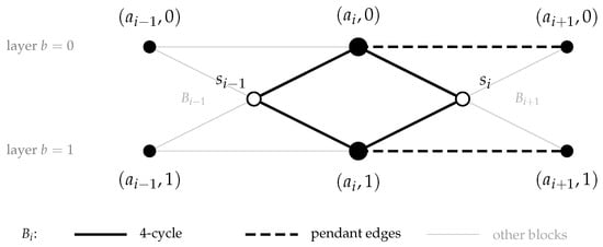
Figure 4 shows the block $B_i$ inside two consecutive pair-gadgets of C.

Figure 4. The block $B_i$ of Lemma 3, drawn inside two consecutive pair gadgets of a cycle. Its 4-cycle (solid heavy) is $\left((a_i,0),s_i,(a_i,1),s_{i-1}\right)$: it takes two edges at each of the shared subdivision vertices $s_{i-1}$ and $s_i$, and its two hubs are the enlarged vertices $(a_i,0)$ and $(a_i,1)$, which sit antipodally on this 4-cycle as Definition 1 requires. Its two pendant edges (heavy dashed) are the clique edges $\{(a_i,0),(a_{i+1},0)\}$ and $\{(a_i,1),(a_{i+1},1)\}$, one in each layer. Every vertex of $B_i$ is therefore visible here: two hubs, the two subdivision vertices in cycle position, and the two leaves on the right. The faint edges belong to $B_{i-1}$ and $B_{i+1}$; each subdivision vertex has degree 4 and splits its edges evenly, with $s_{i-1}$ giving two to $B_{i-1}$ and two to $B_i$ and $s_i$ giving two to $B_i$ and two to $B_{i+1}$. Letting i run over $1,\dots ,r$ therefore covers each of the $6r$ edges of $\Gamma \left(C\right)$ exactly once.

Validity. Both $s_{i-1}=s_{a_{i-1}{a}_i}$ and $s_i=s_{a_i{a}_{i+1}}$ correspond to pairs containing $a_i$, so each is adjacent to $(a_i,0)$ and to $(a_i,1)$; hence,

$$\left((a_i,0),s_i,(a_i,1),s_{i-1}\right)$$

is a genuine 4-cycle. The pendant edges $\{(a_i,0),(a_{i+1},0)\}$ and $\{(a_i,1),(a_{i+1},1)\}$ are the two clique edges of $\Gamma (a_i,a_{i+1})$. The hubs $(a_i,0)$ and $(a_i,1)$ are antipodal on this 4-cycle and have degree 3 in $B_i$, while $s_{i-1},s_i$ have degree 2 and the two leaves degree 1, matching Definition 1. The six vertices are distinct: $s_{i-1}\ne s_i$ as $r\ge 3$; the four clique vertices are distinct as $a_i\ne a_{i+1}$; and subdivision and clique vertices are of different types.

Exact cover. The six edges of $\Gamma (a_i,a_{i+1})$ are used as follows:

$$\begin{array}{c}\underset{\mathrm{cycle}\mathrm{edges}\mathrm{of}{B}_i}{\underbrace{\{s_i,(a_i,0)\},\{s_i,(a_i,1)\}}},\underset{\mathrm{cycle}\mathrm{edges}\mathrm{of}{B}_{i+1}}{\underbrace{\{s_i,(a_{i+1},0)\},\{s_i,(a_{i+1},1)\}}},\\ \underset{\mathrm{pendant}\mathrm{edges}\mathrm{of}{B}_i}{\underbrace{\{(a_i,0),(a_{i+1},0)\},\{(a_i,1),(a_{i+1},1)\}}},\end{array}$$

the middle pair because $s_i$ plays the role $s_{(i+1)-1}$ in $B_{i+1}$. These occurrences are in distinct roles, and, as i runs over $1,\dots ,r$, they exhaust the $6r$ edges of $\Gamma \left(C\right)$ with none repeated. Since $6r/6=r$, the count matches.    □

Lemma 4.

$W(m,2)$ is ${\mathrm{HS}}_6$-decomposable for every $m\ge 3$.

Proof. 

It suffices to decompose $K_m$ into subgraphs F for which $\Gamma \left(F\right)$ is ${\mathrm{HS}}_6$-decomposable. By Lemma 3, every cycle is such an F, and, by the certificates of Section 8, so are $K_4$ and $K_6$ (Lemmas 9 and 11, which decompose $\Gamma \left(K_4\right)=W(4,2)$ and $\Gamma \left(K_6\right)=W(6,2)$). We invoke Veblen’s theorem [21]: a graph decomposes into cycles if and only if every vertex has even degree. Three cases arise.

If m is odd, every vertex of $K_m$ has even degree $m-1$, so $K_m$ itself decomposes into cycles.

If $m\equiv 0(mod4)$, partition $V\left(K_m\right)$ into $m/4$ classes of size 4 and delete a copy of $K_4$ on each. Every vertex loses 3 from its degree, leaving $m-4\equiv 0(mod4)$, which is even, so the remaining complete multipartite graph decomposes into cycles.

If $m\equiv 2(mod4)$, then $m\ge 6$; take one class of size 6 and $(m-6)/4$ classes of size 4, deleting a copy of $K_6$ and copies of $K_4$, respectively. A vertex of the 6-class loses 5, leaving $m-6\equiv 0(mod4)$; a vertex of a 4-class loses 3, leaving $m-4\equiv 2(mod4)$. Both are even, so the remainder again decomposes into cycles.

In each case, $E\left(K_m\right)$ has been partitioned into cycles together with copies of $K_4$ and at most one copy of $K_6$, and every corresponding $\Gamma \left(F\right)$ is ${\mathrm{HS}}_6$-decomposable.    □

Corollary 1.

$W(m,2j)$ is ${\mathrm{HS}}_6$-decomposable for all $m\ge 3$ and $j\ge 1$.

Proof. 

Partition B into j pairs. The edges lying over each pair of layers form a copy of $W(m,2)$; the j copies are edge-disjoint with union $W(m,2j)$. Apply Lemma 4 to each.    □

Corollary 2.

If $m\equiv 1(mod4)$, then $W(m,k)$ is ${\mathrm{HS}}_6$-decomposable for every $k\ge 1$.

Proof. 

The k copies of $K_m^{*}$ that make up $W(m,k)$ are pairwise edge-disjoint, and Theorem 2 gives an ${\mathrm{HS}}_6$-decomposition of each of them.    □

Lemma 5.

$W(4,k)$ is ${\mathrm{HS}}_6$-decomposable for every $k\ge 2$.

Proof. 

Every integer $k\ge 2$ can be written $k=2p+3q$ with $p,q\ge 0$, with the largest integer not so representable being $2·3-2-3=1$. Partition B into p pairs and q triples; the edges over each part form a copy of $W(4,2)$ or of $W(4,3)$, these being edge-disjoint with union $W(4,k)$. Both are ${\mathrm{HS}}_6$-decomposable by Lemmas 9 and 10.    □

7. Proof of the Main Theorem

Proof of Theorem 1. 

Necessity is Proposition 1. For sufficiency, we treat the three admissible residues, applying Lemma 1 in each. The base certificates for $L\left(K_4\right)$ and $L\left(K_5\right)$ are Lemmas 7 and 8.

• Case $n\equiv 1(mod4)$. Induct on n, the base $n=5$ being Lemma 8. For $n\ge 9$, split $n=4+(n-4)$, so that $n-4\equiv 1(mod4)$ and $n-4\ge 5$:

$$L\left(K_n\right)=L\left(K_4\right)\oplus L\left(K_{n-4}\right)\oplus W(4,n-4)\oplus W(n-4,4).$$

Here, $L\left(K_4\right)$ is decomposable by Lemma 7; $L\left(K_{n-4}\right)$ by induction; $W(4,n-4)$ by Lemma 5, since $n-4\ge 5\ge 2$; and $W(n-4,4)$ by Corollary 2, since $n-4\equiv 1(mod4)$.

• Case $n\equiv 2(mod4)$. For $n\ge 6$, split $n=5+(n-5)$, so $n-5\equiv 1(mod4)$:

$$L\left(K_n\right)=L\left(K_5\right)\oplus L\left(K_{n-5}\right)\oplus W(5,n-5)\oplus W(n-5,5).$$

Now, $L\left(K_5\right)$ is decomposable by Lemma 8; $L\left(K_{n-5}\right)$ by the previous case, with this factor being empty when $n=6$; and both glued factors by Corollary 2, since $5\equiv 1$ and $n-5\equiv 1(mod4)$. For $n=6$, the identity reads $L\left(K_6\right)=L\left(K_5\right)\oplus K_5^{*}$, with the second factor being decomposed in Example 1.

• Case $n\equiv 0(mod4)$. Induct on n, with the base $n=4$ being Lemma 7. For $n\ge 8$, split $n=4+(n-4)$, so $n-4\equiv 0(mod4)$ and both 4 and $n-4$ are even:

$$L\left(K_n\right)=L\left(K_4\right)\oplus L\left(K_{n-4}\right)\oplus W(4,n-4)\oplus W(n-4,4),$$

where $L\left(K_{n-4}\right)$ is decomposable by induction and both glued factors by Corollary 1.

Every $n\ge 4$ with $n\not\equiv 3(mod4)$ falls under one of the three cases.    □

Example 2.

(The case $n=9$). Take $n_1=4$, $n_2=5$ in Lemma 1:

$$L\left(K_9\right)=L\left(K_4\right)\oplus L\left(K_5\right)\oplus W(4,5)\oplus W(5,4).$$

The edge counts are $|E\left(L\left(K_9\right)\right)|=9\left({\displaystyle \genfrac{}{}{0pt}{}{8}{2}}\right)=252$ and

$$252=\underset{L\left(K_4\right)}{\underbrace{12}}+\underset{L\left(K_5\right)}{\underbrace{30}}+\underset{W(4,5)=90}{\underbrace{5·3\left({\displaystyle \genfrac{}{}{0pt}{}{4}{2}}\right)}}+\underset{W(5,4)=120}{\underbrace{4·3\left({\displaystyle \genfrac{}{}{0pt}{}{5}{2}}\right)}},$$

giving $252/6=42$ blocks. The first two summands are Lemmas 7 and 8. For $W(4,5)$, write $5=2+3$ and apply Lemma 5, splitting it into one copy of $W(4,2)$ and one of $W(4,3)$. For $W(5,4)$, use Corollary 2: it is four edge-disjoint copies of $K_5^{*}$, each decomposed as in Example 1.

Remark 4.

The recursion is effective: unwinding it yields an explicit block list for every admissible n. We generated and machine-verified these lists for

$$n\in \{4,5,6,8,9,10,12,13,14,16,17,18,20,21,22\},$$

checking in each case that the blocks are copies of ${\mathrm{HS}}_6$, pairwise edge-disjoint, and cover $E\left(L\left(K_n\right)\right)$ exactly.

Remark 5.

(Complexity of the reference implementation). A full, open reference implementation of every construction in this paper—the closed-form $K_m^{*}$ circulant of Theorem 2, the cycle unit and Veblen-based construction of $W(m,2)$ in Lemmas 3 and 4, and the recursive splitting proving Theorem 1 itself—is included in the Supplementary Materials. Since every routine constructs its output explicitly and the output size equals the host’s edge count exactly (Proposition 1), each has time and space complexity matching this count with no asymptotic overhead: $\Theta \left(m^2\right)$ for $K_m^{*}$ and $W(m,2)$, $\Theta \left(k{m}^2\right)$ for $W(m,k)$, and $\Theta \left(n^3\right)$ for $L\left(K_n\right)$, all derived and empirically confirmed in the Supplementary Materials, which also records two genuine implementation defects found and corrected during the analysis and the resulting before/after benchmarks.

8. Base Certificates

This section supplies the five finite decompositions on which the induction rests: $L\left(K_4\right)$, $L\left(K_5\right)$, $W(4,2)$, $W(4,3)$, and $W(6,2)$. We arrange them so that every one can be checked by hand, without software. The certificate for $L\left(K_4\right)$ consists of two blocks and has a structural description (Remark 6). Each of the other four is given as a small number of base blocks together with a cyclic group of automorphisms of the host; the full decomposition is the set of images of the base blocks, and its correctness reduces, by Lemma 6 below, to checking that a single row of 6, or a table of 18, orbit labels contains no repetition. Section 8.1 explains why exactly these five cases are needed, Section 8.2 describes how the base blocks were found, and Section 8.3 lists them. The base blocks were located by computer search, but no part of the verification depends on a computer.

8.1. Why the Induction Needs Exactly These Base Cases

The five certificates are not arbitrary small cases: each marks a point at which one of the general constructions of Section 4, Section 5 and Section 6 provably cannot be applied as it stands, so the induction must be anchored there.

(i)

$L\left(K_4\right)$ and $L\left(K_5\right)$. The proof of Theorem 1 reduces $L\left(K_n\right)$ through Lemma 1 to summands that are decomposed separately. For $n=4$ and $n=5$, every splitting $n=n_1+n_2$ produces a summand that has no ${\mathrm{HS}}_6$-decomposition: for $n=4$, the split $1+3$ produces $L\left(K_3\right)\cong K_3$, with 3 edges, and the split $2+2$ produces $W(2,2)$, whose six edges form two triangles sharing the vertex $s_{01}$ (a bowtie, not a copy of ${\mathrm{HS}}_6$); for $n=5$, the split $1+4$ produces $W(4,1)=K_4^{*}$, excluded by Theorem 3, and the split $2+3$ again produces $L\left(K_3\right)$. Hence, $L\left(K_4\right)$ and $L\left(K_5\right)$ cannot be reached by the splitting method and must be decomposed directly.

(ii)

$W(4,2)$ and $W(6,2)$. Lemma 4 turns a decomposition of $K_m$ into subgraphs F into one of $W(m,2)$, provided that each $\Gamma \left(F\right)$ is decomposable, and Lemma 3 supplies every cycle as such an F. When m is even, every vertex of $K_m$ has odd degree, so, by Veblen’s theorem, cycles alone cannot cover $K_m$: some subgraph F in which every vertex has odd degree must be absorbed separately. The simplest choice, a perfect matching, fails, since, for a single edge, $\Gamma \left(K_2\right)=W(2,2)$ is the bowtie just mentioned. We use instead vertex-disjoint copies of $K_4$, all of whose degrees are odd; as $K_4$ has no cycle decomposition, $\Gamma \left(K_4\right)=W(4,2)$ is not reachable by Lemma 3 and must be decomposed directly. When $m\equiv 2(mod4)$, the vertex set cannot be partitioned into 4-sets, and one copy of $K_6$, again with all degrees odd, absorbs the remaining residue, giving the base case $W(6,2)$.

(iii)

$W(4,3)$. In the case $n\equiv 1(mod4)$, the splitting $n=4+(n-4)$ produces $W(4,n-4)$ with $n-4$ odd. Even layer counts are handled by pairing layers (Corollary 1), and Corollary 2 does not apply because $4\not\equiv 1(mod4)$. An odd number of layers therefore requires one block of an odd number of layers; one layer, $W(4,1)=K_4^{*}$, is impossible by Theorem 3, so three layers is the least possible, and $W(4,3)$ is the corresponding base case (Lemma 5).

In each case, the obstruction that blocks the general construction, namely too few vertices to split, odd degrees for Veblen’s theorem, and the rigidity of a single triangle bundle, is exactly what the corresponding certificate overcomes. The certificates themselves are small but not structureless: $L\left(K_4\right)$ has exactly six ${\mathrm{HS}}_6$-decompositions, all equivalent under the action of $S_4$ on the indices and all of the form described in Remark 6, and the other four are invariant under the cyclic groups exhibited below.

8.2. How the Base Blocks Were Found

The base blocks were located by a short exact search, which we describe so that it can be reproduced independently; its output is, in any case, checked by hand in Section 8.3.

Step 1: Candidate blocks. For a host G, we enumerate all copies of ${\mathrm{HS}}_6$ in G by choosing a hub $w_0$, two of its neighbours $w_1,w_3$, and a common neighbour $w_2\ne w_0$ of $w_1$ and $w_3$ and leaves $m_0\in N\left(w_0\right)\setminus \{w_1,w_2,w_3\}$ and $m_2\in N\left(w_2\right)\setminus \{w_0,w_1,w_3,m_0\}$; duplicates arising from the symmetries of ${\mathrm{HS}}_6$ are removed by storing each copy as its edge set. This takes $O\left(\right|V\left(G\right)|\Delta {\left(G\right)}^4)$ time, where $\Delta \left(G\right)$ is the maximum degree.

Step 2: Symmetry reduction. We fix a group $\mathcal{G}$ of automorphisms of G that acts semiregularly on $E\left(G\right)$, compute the $\left|E\right(G\left)\right|/\left|\mathcal{G}\right|$ edge orbits, and keep only those candidates whose six edges lie in six distinct orbits; by Lemma 6, these are exactly the admissible base blocks.

Step 3: Exact cover. We seek $t=\left|E\right(G\left)\right|/\left(6\right|\mathcal{G}\left|\right)$ admissible base blocks that cover every orbit exactly once. This is an instance of the exact cover problem, solved by depth-first backtracking that always branches on an uncovered orbit lying in the fewest remaining candidates, as in Knuth’s Algorithm X. The only constraints are as follows: each block is a copy of ${\mathrm{HS}}_6$, with degree sequence $(3,3,2,2,1,1)$, non-adjacent hubs, and distinct leaves; its six edges lie in distinct orbits; and the chosen blocks cover each orbit exactly once.

Complexity and running time. Exact cover is NP-complete, and the ${\mathrm{HS}}_6$-decomposition problem itself is NP-complete [7], so no polynomial bound is claimed for Step 3. At the present sizes, however, the search is immediate, as Table 1 shows (Python 3.13, single core, x86-64). For $L\left(K_4\right)$, no group was needed, and the search over all 48 copies of ${\mathrm{HS}}_6$ in $L\left(K_4\right)$ also yields the count of six decompositions quoted above. For $W(4,2)$ and $W(4,3)$, some natural groups admit no invariant decomposition; for instance, $W(4,2)$ has none invariant under ${\mathbb{Z}}_3$ acting on three of its four points or under the bare exchange of its two layers. These negative outcomes, recorded in the Supplementary Materials, are not used anywhere in the proofs.

Table 1. The certificate search. “Copies of ${\mathrm{HS}}_6$” counts all copies in the host (Step 1); “admissible” counts those with edges in six distinct orbits (Step 2); “search nodes” counts the calls of the backtracking procedure of Step 3 up to the first solution. Candidates and orbits are processed in a fixed (sorted) order, so the node counts are reproducible; times include Steps 1–3 and are medians of five runs of the script hs6_symmetric_search.py in the Supplementary Materials.

Host G	$\left|\mathit{E}\right(\mathit{G}\left)\right|$	Group $\mathcal{G}$	Orbits	Copies of ${\mathbf{HS}}_6$	Admissible	Search Nodes	Time
$L\left(K_4\right)$	12	trivial	12	48	48	6	<1 ms
$L\left(K_5\right)$	30	${\mathbb{Z}}_5$	6	1980	40	2	32 ms
$W(4,2)$	36	$⟨\sigma ⟩\cong {\mathbb{Z}}_2$	18	708	584	61	10 ms
$W(4,3)$	54	${\mathbb{Z}}_3$	18	2088	1629	18	32 ms
$W(6,2)$	90	${\mathbb{Z}}_5$	18	19,620	4490	7	453 ms

8.3. The Certificates

• Notation. In Lemmas 7 and 8, the symbol $ij$ denotes the vertex of $L\left(K_n\right)$ corresponding to the edge $\{i,j\}$ of $K_n$, with two such vertices being adjacent when they share an index. For $W(m,k)$, we write $a_b$ for the clique vertex $(a,b)$ and $s_{a{a}^{\prime }}$ for the shared subdivision vertex, following Definition 3. Since $W(m,k)$ depends only on the size of its point set, for $W(4,3)$ and $W(6,2)$, we take the point set to be ${\mathbb{Z}}_3\cup \{\infty \}$ and ${\mathbb{Z}}_5\cup \{\infty \}$, respectively. Each block is written as in Definition 1; in the tables, the six columns list the edges of a block in the fixed order $\{w_0,w_1\},\{w_1,w_2\},\{w_2,w_3\},\{w_3,w_0\}$ (the 4-cycle) and $\{w_0,m_0\},\{w_2,m_2\}$ (the two pendant edges).

Lemma 6.

(Development of base blocks). Let $\mathcal{G}$ be a group of automorphisms of a graph G that acts semiregularly on $E\left(G\right)$, i.e., no non-identity element of $\mathcal{G}$ maps an edge to itself. Let $B_1,\dots ,B_t$ be copies of ${\mathrm{HS}}_6$ in G such that the $6t$ edges of $B_1\cup \cdots \cup B_t$ lie in pairwise distinct $\mathcal{G}$-orbits, and every $\mathcal{G}$-orbit on $E\left(G\right)$ contains one of them. Then,

$$\mathcal{D}=\{\gamma \left(B_i\right):\gamma \in \mathcal{G},1\le i\le t\}$$

is an ${\mathrm{HS}}_6$-decomposition of G with $t\left|\mathcal{G}\right|$ blocks; equivalently, $\left|E\right(G\left)\right|=6t\left|\mathcal{G}\right|$.

Proof. 

Each $\gamma \left(B_i\right)$ is a copy of ${\mathrm{HS}}_6$, since $\gamma$ is an automorphism. Let $e\in E\left(G\right)$. By hypothesis, the orbit $\mathcal{G}e$ contains exactly one edge f of the base blocks—say, $f\in B_i$—and, by semiregularity, there is exactly one $\gamma \in \mathcal{G}$ with $\gamma \left(f\right)=e$; thus, $e\in \gamma \left(B_i\right)$. Conversely, if $e\in {\gamma }^{\prime }\left(B_j\right)$, then $e={\gamma }^{\prime }\left(f^{\prime }\right)$ for some edge $f^{\prime }$ of $B_j$, so $f^{\prime }\in \mathcal{G}e$, whence $f^{\prime }=f$, $j=i$ and ${\gamma }^{\prime }=\gamma$. Hence, every edge of G lies in exactly one member of $\mathcal{D}$, and the members of $\mathcal{D}$ are distinct.    □

In each application below, the hand check therefore has two parts: (a) we confirm that $\mathcal{G}$ is semiregular on edges, which is a one-line argument given in each proof; and (b) we confirm that the orbit labels in the accompanying table are pairwise distinct and that their number, $6t$, equals the number $\left|E\right(G\left)\right|/\left|\mathcal{G}\right|$ of orbits. That each listed base block is a copy of ${\mathrm{HS}}_6$ inside the host is read off directly from the array.

Lemma 7.

${\mathrm{HS}}_6\mid L\left(K_4\right)$.

Proof. 

The $\left({\displaystyle \genfrac{}{}{0pt}{}{4}{2}}\right)·2/6=2$ blocks

$$\begin{array}{c}\left(\begin{array}{ccccc}& 12& & 03& \\ 23& 13& 01& 02& 23\end{array}\right),\left(\begin{array}{ccccc}& 23& & 01& \\ 03& 02& 12& 13& 03\end{array}\right)\end{array}$$

are copies of ${\mathrm{HS}}_6$ in $L\left(K_4\right)$, and together they use each of the 12 edges of $L\left(K_4\right)$ exactly once; Remark 6 below explains why.    □

Remark 6.

This certificate has a direct structural explanation, which we record because it is not visible from the block list alone. $L\left(K_4\right)$ is isomorphic to the octahedron graph $K_{2,2,2}$, whose three independent sets of size 2 are exactly the three pairs of disjoint edges of $K_4$: $A=\{01,23\}$, $B=\{02,13\}$, $C=\{03,12\}$. Under this identification, the first block above uses all of A as its two hubs, all of B as the remaining two cycle vertices, and all of C as its two leaves; the second block rotates the roles, using C as hubs and A as leaves, while B again supplies the cycle vertices. Every edge between A and B, and between B and C, is used exactly once as a cycle edge; every edge between A and C is used exactly once, split between the two blocks’ pendant edges. For the remaining four certificates, we give, in place of a structural explanation, a presentation under a group of automorphisms that reduces their verification to a short hand check (Lemma 6).

Lemma 8.

${\mathrm{HS}}_6\mid L\left(K_5\right)$.

Proof. 

Let $\mathcal{G}={\mathbb{Z}}_5$ act on $L\left(K_5\right)$ through $x\mapsto x+1$ on the indices $\{0,\dots ,4\}$. An edge of $L\left(K_5\right)$ has the form $\{xy,xz\}$ with $x,y,z$ distinct; its shared index x is unique, and a translation by $t\ne 0$ moves it to $x+t\ne x$, so $\mathcal{G}$ is semiregular on the 30 edges, with $30/5=6$ orbits. We label the edge $\{xy,xz\}$ by the unordered pair $\{y-x,z-x\}$ of distinct elements of ${\mathbb{Z}}_5\setminus \left\{0\right\}$. This label is unchanged by translation and, together with x, determines the edge, so the six orbits correspond bijectively to the $\left({\displaystyle \genfrac{}{}{0pt}{}{4}{2}}\right)=6$ possible labels $\{1,2\},\{1,3\},\{1,4\},\{2,3\},\{2,4\},\{3,4\}$.

Table 2 gives a single base block and the labels of its six edges, which are the six possible labels, each exactly once. By Lemma 6, the five images of this block under $\mathcal{G}$ form an ${\mathrm{HS}}_6$-decomposition of $L\left(K_5\right)$ with $30/6=5$ blocks.    □

Table 2. Base block for Lemma 8: $L\left(K_5\right)$ under $\mathcal{G}={\mathbb{Z}}_5$, with the orbit label of each edge.

Base Block	$\{{\mathit{w}}_0,{\mathit{w}}_1\}$	$\{{\mathit{w}}_1,{\mathit{w}}_2\}$	$\{{\mathit{w}}_2,{\mathit{w}}_3\}$	$\{{\mathit{w}}_3,{\mathit{w}}_0\}$	$\{{\mathit{w}}_0,{\mathit{m}}_0\}$	$\{{\mathit{w}}_2,{\mathit{m}}_2\}$
$\left(\begin{array}{ccccc}& 02& & 01& \\ 23& 34& 14& 24& 23\end{array}\right)$	$\{1,4\}$	$\{2,4\}$	$\{2,3\}$	$\{1,2\}$	$\{1,3\}$	$\{3,4\}$

Lemma 9.

${\mathrm{HS}}_6\mid W(4,2)$.

Proof. 

Let $\mathcal{G}=\{1,\sigma \}$, where $\sigma$ is the involution

$$\sigma \left(a_b\right)=\pi {\left(a\right)}_{1-b},\sigma \left(s_{a{a}^{\prime }}\right)=s_{\pi \left(a\right)\pi \left(a^{\prime }\right)},\pi =\left(01\right)\left(23\right).$$

Every edge of $W(4,2)$ has at least one clique endpoint, and $\sigma$ moves every clique vertex to the other layer; so $\sigma$ fixes no edge, and $\mathcal{G}$ is semiregular with $36/2=18$ orbits. Each orbit has exactly one edge in layer 0, and we label an edge by this representative: the edge itself if its clique endpoints are in layer 0, otherwise its image under $\sigma$. A label $a{a}^{\prime }$ denotes the clique edge $\{a_0,a_0^{\prime }\}$ and a label $a-s_{a{a}^{\prime }}$ the subdivision edge $\{a_0,s_{a{a}^{\prime }}\}$. The 18 labels are thus the edges of the layer-0 copy of $K_4^{*}$: the six clique edges $01,02,03,12,13,23$ and the twelve subdivision edges $a-s_{a{a}^{\prime }}$.

Table 3 gives three base blocks and the labels of their 18 edges, which list each of these 18 labels exactly once. By Lemma 6, the three base blocks and their images under $\sigma$ form an ${\mathrm{HS}}_6$-decomposition of $W(4,2)$ with $36/6=6$ blocks.    □

Table 3. Base blocks for Lemma 9: $W(4,2)$ under $\mathcal{G}=⟨\sigma ⟩\cong {\mathbb{Z}}_2$, with the orbit label of each edge.

Base Block	$\{{\mathit{w}}_0,{\mathit{w}}_1\}$	$\{{\mathit{w}}_1,{\mathit{w}}_2\}$	$\{{\mathit{w}}_2,{\mathit{w}}_3\}$	$\{{\mathit{w}}_3,{\mathit{w}}_0\}$	$\{{\mathit{w}}_0,{\mathit{m}}_0\}$	$\{{\mathit{w}}_2,{\mathit{m}}_2\}$
$\left(\begin{array}{ccccc}& 2_0& & 1_1& \\ 3_0& s_{23}& 3_1& s_{13}& 3_0\end{array}\right)$	$3-s_{23}$	$2-s_{23}$	$2-s_{02}$	$3-s_{13}$	23	02
$\left(\begin{array}{ccccc}& 3_0& & 3_1& \\ 0_0& s_{01}& 0_1& s_{02}& 0_0\end{array}\right)$	$0-s_{01}$	$1-s_{01}$	$1-s_{13}$	$0-s_{02}$	03	12
$\left(\begin{array}{ccccc}& s_{12}& & 3_1& \\ 1_0& 3_0& s_{03}& 0_0& 1_0\end{array}\right)$	13	$3-s_{03}$	$0-s_{03}$	01	$1-s_{12}$	$2-s_{12}$

Lemma 10.

${\mathrm{HS}}_6\mid W(4,3)$.

Proof. 

Take the point set ${\mathbb{Z}}_3\cup \{\infty \}$ and layer indices in ${\mathbb{Z}}_3$, and let $\mathcal{G}=⟨\tau ⟩\cong {\mathbb{Z}}_3$, where

$$\tau \left(a_b\right)={(a+1)}_{b+1}(a\in {\mathbb{Z}}_3),\tau \left({\infty }_b\right)={\infty }_{b+1},\tau \left(s_{uv}\right)=s_{\tau u\tau v},$$

with $\infty +1=\infty$. Every edge has a clique endpoint, and $\tau$ and ${\tau }^2$ change the layer of every clique vertex, so $\mathcal{G}$ is semiregular with $54/3=18$ orbits. With r denoting a residue modulo 3, we use the labels $C\left(r\right)$ for the clique edge $\{a_b,{(a+1)}_b\}$, $C_{\infty }\left(r\right)$ for $\{a_b,{\infty }_b\}$, $S_d\left(r\right)$ for $\{a_b,s_{a,a+d}\}$ with $d\in \{1,2\}$, $S_{\infty }\left(r\right)$ for $\{a_b,s_{a\infty }\}$, and $T\left(r\right)$ for $\{{\infty }_b,s_{a\infty }\}$, where in each case $r=b-a$. Every pair in ${\mathbb{Z}}_3$ is $\{a,a+1\}$ for exactly one a, so each label is well defined; each is invariant under $\tau$, since $\tau$ adds 1 to both a and b; and a label together with the layer b determines the edge. The labels therefore correspond bijectively to the orbits, and there are $3+3+6+3+3=18$ of them.

Table 4 gives three base blocks and the labels of their 18 edges, which list each of the 18 labels exactly once. By Lemma 6, the three base blocks and their images under $\tau$ and ${\tau }^2$ form an ${\mathrm{HS}}_6$-decomposition of $W(4,3)$ with $54/6=9$ blocks.    □

Table 4. Base blocks for Lemma 10: $W(4,3)$ under $\mathcal{G}=⟨\tau ⟩\cong {\mathbb{Z}}_3$, with the orbit label of each edge.

Base Block	$\{{\mathit{w}}_0,{\mathit{w}}_1\}$	$\{{\mathit{w}}_1,{\mathit{w}}_2\}$	$\{{\mathit{w}}_2,{\mathit{w}}_3\}$	$\{{\mathit{w}}_3,{\mathit{w}}_0\}$	$\{{\mathit{w}}_0,{\mathit{m}}_0\}$	$\{{\mathit{w}}_2,{\mathit{m}}_2\}$
$\left(\begin{array}{ccccc}& {\infty }_1& & 1_0& \\ s_{2\infty }& {\infty }_0& 0_0& 2_0& s_{2\infty }\end{array}\right)$	$T\left(1\right)$	$C_{\infty }\left(0\right)$	$C\left(1\right)$	$S_{\infty }\left(1\right)$	$T\left(2\right)$	$C\left(0\right)$
$\left(\begin{array}{ccccc}& 2_0& & s_{1\infty }& \\ s_{02}& 0_1& {\infty }_1& 2_1& s_{02}\end{array}\right)$	$S_2\left(1\right)$	$C_{\infty }\left(1\right)$	$C_{\infty }\left(2\right)$	$S_1\left(2\right)$	$S_1\left(1\right)$	$T\left(0\right)$
$\left(\begin{array}{ccccc}& s_{01}& & 1_2& \\ 0_0& s_{02}& 0_2& s_{0\infty }& 0_0\end{array}\right)$	$S_2\left(0\right)$	$S_2\left(2\right)$	$S_{\infty }\left(2\right)$	$S_{\infty }\left(0\right)$	$S_1\left(0\right)$	$C\left(2\right)$

Lemma 11.

${\mathrm{HS}}_6\mid W(6,2)$.

Proof. 

Take the point set ${\mathbb{Z}}_5\cup \{\infty \}$, and let $\mathcal{G}={\mathbb{Z}}_5$ act by $a\mapsto a+1$ on ${\mathbb{Z}}_5$, fixing ∞ and both layers. Every edge of $W(6,2)$ contains a vertex indexed by some $a\in {\mathbb{Z}}_5$ (a clique vertex $a_b$ or a subdivision vertex $s_{a{a}^{\prime }}$ with $a\in {\mathbb{Z}}_5$), which a non-trivial translation moves; and since $\mathcal{G}$ has odd order, no element can interchange the two ends of an edge. So $\mathcal{G}$ is semiregular with $90/5=18$ orbits. With $b\in \{0,1\}$ denoting the layer, we use the labels $C_d\left(b\right)$ for the clique edge $\{a_b,{(a\pm d)}_b\}$ with $d\in \{1,2\}$, $C_{\infty }\left(b\right)$ for $\{a_b,{\infty }_b\}$, $S_d\left(b\right)$ for $\{a_b,s_{a,a+d}\}$ with $d\in \{1,2,3,4\}$, $S_{\infty }\left(b\right)$ for $\{a_b,s_{a\infty }\}$, and $T\left(b\right)$ for $\{{\infty }_b,s_{a\infty }\}$. The labels are translation-invariant and, together with one index a, determine the edge, so they correspond bijectively to the orbits; there are $4+2+8+2+2=18$ of them.

Table 5 gives three base blocks and the labels of their 18 edges, which list each of the 18 labels exactly once. By Lemma 6, the three base blocks and their images under the translations $a\mapsto a+t$, $t=1,\dots ,4$, form an ${\mathrm{HS}}_6$-decomposition of $W(6,2)$ with $90/6=15$ blocks.    □

Table 5. Base blocks for Lemma 11: $W(6,2)$ under $\mathcal{G}={\mathbb{Z}}_5$ (fixing ∞), with the orbit label of each edge.

Base Block	$\{{\mathit{w}}_0,{\mathit{w}}_1\}$	$\{{\mathit{w}}_1,{\mathit{w}}_2\}$	$\{{\mathit{w}}_2,{\mathit{w}}_3\}$	$\{{\mathit{w}}_3,{\mathit{w}}_0\}$	$\{{\mathit{w}}_0,{\mathit{m}}_0\}$	$\{{\mathit{w}}_2,{\mathit{m}}_2\}$
$\left(\begin{array}{ccccc}& 3_1& & {\infty }_0& \\ 2_1& {\infty }_1& s_{0\infty }& 0_1& 2_1\end{array}\right)$	$C_{\infty }\left(1\right)$	$T\left(1\right)$	$S_{\infty }\left(1\right)$	$C_2\left(1\right)$	$C_1\left(1\right)$	$T\left(0\right)$
$\left(\begin{array}{ccccc}& {\infty }_0& & s_{01}& \\ 1_0& s_{14}& 1_1& s_{13}& 1_0\end{array}\right)$	$S_3\left(0\right)$	$S_3\left(1\right)$	$S_2\left(1\right)$	$S_2\left(0\right)$	$C_{\infty }\left(0\right)$	$S_4\left(1\right)$
$\left(\begin{array}{ccccc}& s_{1\infty }& & 2_1& \\ 1_0& 2_0& s_{23}& 3_0& 1_0\end{array}\right)$	$C_1\left(0\right)$	$S_1\left(0\right)$	$S_4\left(0\right)$	$C_2\left(0\right)$	$S_{\infty }\left(0\right)$	$S_1\left(1\right)$

9. Concluding Remarks

Two features of the argument seem worth isolating. First, the obstruction of Theorem 3 is real but fragile: it is destroyed the moment that two triangle bundles are glued along their degree-two vertices, which is precisely the configuration produced by the splitting identity. Second, Lemma 3 converts any cycle decomposition of $K_m$ into an ${\mathrm{HS}}_6$-decomposition of $W(m,2)$, so that Veblen’s theorem performs all the work for odd m, while two small certificates absorb the parity defect for even m.

Several directions suggest themselves. The same programme should apply to the higher members ${\mathrm{HS}}_{3k}$ of the family, whose decompositions of the complete and complete multipartite hosts are studied in [18]; the next case is the nine-vertex graph obtained from a hexagon by attaching pendant edges at three alternating vertices. Lemma 1 is independent of the pattern graph and transfers unchanged, so what must be redone is the analysis of $K_m^{*}$ and of the glued graphs $W(m,k)$, where the analogue of the cycle unit of Lemma 3 is the natural starting point. Since $\left|E\right({\mathrm{HS}}_{3k}\left)\right|=3k$, one expects the arithmetic to be governed by the prime factorisation of $3k$ and, in particular, the case $k=3$, where $\left|E\right|=9$ is a prime power, to behave differently from the case $k=2$ treated here. One may also ask for $\{{\mathrm{HS}}_6^{\alpha },C_4^{\beta }\}$-multidecompositions of $L\left(K_n\right)$ in the spirit of [17], with the 4-cycle already sitting inside every block.

Finally, since $L\left(K_n\right)$ is the case $\lambda =1$ of the $\lambda$-fold line graph, the corresponding question for $\lambda \ge 2$ remains open. Two data points make this direction concrete rather than purely speculative: Ganesamurthy and Paulraja [14] settled the $C_5$ case, and Zhao, Wei, and Yang [16] settled the $C_4$-decomposability of the $\lambda$-fold line graph of the complete bipartite graph $K_{m,n}$—a different host but the same $\lambda$-fold mechanism. Both results suggest that $\lambda$-fold line-graph decomposition problems tend to admit clean answers once the $\lambda =1$ case is understood, which is some evidence that an ${\mathrm{HS}}_6$-decomposition characterisation for $\lambda L\left(K_n\right)$, $\lambda \ge 2$, is within reach of the methods described in this paper; we have not attempted it here.

References

- Alspach, B.; Gavlas, H. Cycle decompositions of Kn and Kn-I. J. Combin. Theory Ser. B 2001, 81, 77–99. [Google Scholar]
- Bryant, D.; Horsley, D.; Pettersson, W. Cycle decompositions V: Complete graphs into cycles of arbitrary lengths. Proc. Lond. Math. Soc. 2014, 108, 1153–1192. [Google Scholar] [CrossRef] [Scilit]
- Sotteau, D. Decomposition of Km,n () into cycles (circuits) of length 2k. J. Comb. Theory Ser. B 1981, 30, 75–81. [Google Scholar] [CrossRef] [Scilit]
- Cameron, R.A.; Horsley, D. Decompositions of complete multigraphs into stars of varying sizes. J. Comb. Theory Ser. B 2020, 145, 32–64. [Google Scholar] [CrossRef] [Scilit]
- Shyu, T.-W. Decompositions of complete bipartite graphs and complete graphs into paths, stars, and cycles with four edges each. Discuss. Math. Graph Theory 2021, 41, 451–468. [Google Scholar] [CrossRef] [Scilit]
- Sethuraman, G.; Murugan, V. Decomposition of complete graphs into arbitrary trees. Graphs Comb. 2021, 37, 1191–1203. [Google Scholar] [CrossRef] [Scilit]
- Dor, D.; Tarsi, M. Graph decomposition is NP-complete: A complete proof of Holyer’s conjecture. SIAM J. Comput. 1997, 26, 1166–1187. [Google Scholar] [CrossRef] [Scilit]
- Colby, M.; Rodger, C.A. Cycle decompositions of the line graph of Kn. J. Comb. Theory Ser. A 1993, 62, 158–161. [Google Scholar] [CrossRef] [Scilit]
- Cox, B.A. The complete spectrum of 6-cycle systems of L(Kn). J. Comb. Des. 1995, 3, 353–362. [Google Scholar] [CrossRef] [Scilit]
- Cox, B.A.; Rodger, C.A. Cycle systems of the line graph of the complete graph. J. Graph Theory 1996, 21, 173–182. [Google Scholar] [CrossRef] [Scilit]
- Xin, Y.; Yang, W. Decomposition of the line graph of the complete graph into stars. Discret. Math. 2024, 347, 114026. [Google Scholar] [CrossRef] [Scilit]
- Heinrich, K.; Nonay, G. Exact coverings of 2-paths by 4-cycles. J. Comb. Theory Ser. A 1987, 45, 50–61. [Google Scholar] [CrossRef] [Scilit]
- Verrall, H. A construction of a perfect set of Euler tours of K2k + I. J. Comb. Des. 1998, 6, 183–211. [Google Scholar] [CrossRef] [Scilit]
- Ganesamurthy, S.; Paulraja, P. A C5-decomposition of the λ-fold line graph of the complete graph. Discret. Math. 2019, 342, 2197–2210. [Google Scholar]
- Ganesamurthy, S.; Paulraja, P.; Srimathi, R. Multidecompositions of line graphs of complete graphs. Discret. Math. Algorithms Appl. 2019, 11, 1950035. [Google Scholar] [CrossRef] [Scilit]
- Zhao, Y.; Wei, Y.; Yang, W. A C4-decomposition of the λ-fold line graph of Km,n. arXiv 2022, arXiv:2205.05117. [Google Scholar]
- Ganesamurthy, S. Decompositions of line graphs of complete graphs into paths and cycles. Discret. Math. 2023, 346, 113165. [Google Scholar] [CrossRef] [Scilit]
- Palaniyandi, G.; Soundararajan, A.; Soundararajan, S. Decomposition of complete, complete bipartite, and complete tripartite graphs into half-sunlet graphs of order twelve. Mathematics 2026, 14, 3354. [Google Scholar] [CrossRef] [Scilit]
- Boulet, R. Spectral characterizations of sun graphs and broken sun graphs. Discret. Math. Theor. Comput. Sci. 2009, 11, 149–160. [Google Scholar] [CrossRef] [Scilit]
- Rather, B.A.; Ganie, H.A.; Shang, Y. Distance Laplacian spectral ordering of sun type graphs. Appl. Math. Comput. 2023, 445, 127847. [Google Scholar] [CrossRef] [Scilit]
- Veblen, O. An application of modular equations in analysis situs. Ann. Math. 1912, 14, 86–94. [Google Scholar] [CrossRef] [Scilit]
Disclaimer/Publisher’s Note: The statements, opinions and data contained in all publications are solely those of the individual author(s) and contributor(s) and not of MDPI and/or the editor(s). MDPI and/or the editor(s) disclaim responsibility for any injury to people or property resulting from any ideas, methods, instructions or products referred to in the content. |
© 2026 by the authors. Licensee MDPI, Basel, Switzerland. This article is an open access article distributed under the terms and conditions of the Creative Commons Attribution (CC BY) license.