On Matrix Linear Diophantine Equation-Based Digital-Adaptive Block Pole Placement Control for Multivariable Large-Scale Linear Process

Abstract

This paper introduces a digital adaptive control framework for large-scale multivariable systems, integrating matrix linear Diophantine equations with block pole placement. The main innovation lies in adaptively relocating the full eigenstructure using matrix polynomial representations and a recursive identification algorithm for real-time parameter estimation. The proposed method achieves accurate eigenvalue placement, strong disturbance rejection, and fast regulation under model uncertainty. Its effectiveness is demonstrated through simulations on a large-scale winding process, showing precise tracking, low steady-state error, and robust decoupling. Compared with traditional non-adaptive designs, the approach ensures superior performance against parameter variations and noise, highlighting its potential for high-performance industrial applications.

1. Introduction

The design of adaptive multivariable controllers has progressed substantially with advances in model identification, pole placement theory, and computational control methods. Early studies [1,2,3] introduced instrumental and prediction-error techniques for identifying Linear matrix fraction description (LMFD) models, providing a structured foundation for multivariable system representation. Building on these principles [4], later works extended polynomial eigenvalue formulations to MIMO systems [5,6,7], offering deeper insights into eigenstructure assignment. Foundational research on matrix polynomials and interpolation [8,9,10,11] was further developed in the context of industrial multivariable process identification [12,13,14]. These contributions paved the way for adaptive control schemes such as [15], which integrate recursive estimation and robust design strategies [16,17,18]. Classical control theory [19,20,21] emphasized the role of controllability and observability in pole assignment, while mathematical formulations [22,23,24,25] provided Diophantine and polynomial equation solutions essential for digital control and their application to block pole placement in winding processes [26,27]. More advanced matrix polynomial approaches [28,29,30,31] enabled robust block structure relocation and eigenvalue assignment, supported by system-theoretic formulations and modeling tools [32,33,34,35,36] that facilitated practical MIMO compensator synthesis. Classical non-adaptive control methods, though well established, degrade under parameter variations, model uncertainties, and external disturbances. Their reliance on fixed compensator structures and focus on eigenvalue assignment limit flexibility in shaping the full eigenstructure and reduce robustness in multivariable systems. To address these issues, the proposed approach employs a matrix linear Diophantine framework with adaptive block pole placement, enabling online parameter adjustment and accurate eigenstructure assignment under uncertainty. Recent works [37,38,39,40,41] have explored neural network control, optimization, and AI-assisted pole placement for nonlinear and large-scale systems. In this context, the present study introduces an adaptive digital block pole placement strategy tailored to large-scale MIMO winding processes, ensuring precise closed-loop performance under real-time conditions.

This paper proposes a novel design methodology for MIMO adaptive compensators, offering greater flexibility in assigning system eigenstructure through block poles. Unlike conventional approaches, this method enables the placement of more than just the original set of desired eigenvalues, thereby enhancing the robustness and performance of digital MIMO control systems. To the best of the authors’ knowledge, previous research has not explored adaptive block pole placement in digital systems represented by matrix fractions for eigenstructure assignment via dynamic compensators. This paper is structured as follows. Section 2 reviews existing MIMO system identification algorithms. Section 3 introduces the proposed adaptive block pole placement technique using digital compensator design. In Section 4, an application to the discrete adaptive control of a winding process is presented to demonstrate the effectiveness of the method. Finally, Section 5 provides concluding remarks and potential future research directions.

2. Theoretical Preliminaries for MIMO Polynomial Systems

2.1. Operator-Theoretic Foundations

This section provides the math-foundation for the proposed method, presenting operator-theoretic concepts, rational matrix-valued functions, spectral projectors, and other related algebraic topics. These tools are essential for analyzing matrix polynomial systems and designing compensators by allowing $\mathrm{e}\mathrm{i}\mathrm{g}\mathrm{e}\mathrm{n}\mathrm{s}\mathrm{t}\mathrm{r}\mathrm{u}\mathrm{c}\mathrm{t}\mathrm{u}\mathrm{r}\mathrm{e}$ assignment. The $\mathrm{e}\mathrm{i}\mathrm{g}\mathrm{e}\mathrm{n}\mathrm{s}\mathrm{p}\mathrm{a}\mathrm{c}\mathrm{e}$ decomposition and projector-based techniques define the spectral structure of the closed-loop system. High-order difference systems (polynomial operators) often involve large-dimensional matrices, which has led to a renewed interest in rational matrix polynomial and state-space representations [42]. Polynomial systems theory in discrete time relies on the properties of polynomial matrices over the shift operator, using polynomial operator algebra (a natural extension of classical operational calculus based on the z-transform). To clarify these concepts, consider the finite-dimensional Hilbert spaces $\mathcal{U}$ and $\mathcal{Y}$ representing the input and output spaces, respectively. Let the forward shift operator $\sigma$ be defined by $\sigma \left(x\left[k\right]\right)=x\left[k+1\right]$, understood as a bounded linear shift operator on a sequence space $\mathcal{D}\left(\sigma \right)\subset {\mathbb{L}}^2\left(\mathbb{Z},\mathcal{U}\right)$. Two operator-valued matrix polynomials are defined: $D_L\left(\sigma \right)=\sum _{i=0}^{\mathsf{\ell }}{D}_{L\mathit{i}}{\sigma }^{\mathsf{\ell }-\mathit{i}}\in \mathcal{B}\left(\mathcal{Y}\right)$ and $N_L\left(\sigma \right)=\sum _{i=0}^{\mathsf{\ell }}{N}_{Li}{\sigma }^{\mathsf{\ell }-\mathit{i}}\in \mathcal{B}\left(\mathcal{U},\mathcal{Y}\right)$, where $D_{Li}\in {\mathbb{R}}^{p\times p}\subset \mathcal{B}\left(\mathcal{Y}\right)$, $N_{Li}\in {\mathbb{R}}^{p\times m}\subset \mathcal{B}\left(\mathcal{U},\mathcal{Y}\right)$, and $\mathcal{B}\left(.\right)$ denotes the space of bounded linear operators between corresponding spaces. The discrete-time polynomial system can be formalized as $D_L\left(\sigma \right)y\left[k\right]=N_L\left(\sigma \right)u\left[k\right]$, with $u\left[k\right]\in \mathcal{D}\left(N_L\left(\sigma \right)\right)$ and $y\left[k\right]\in \mathcal{D}\left(D_L\left(\sigma \right)\right)$, both contained in appropriate sequence spaces (e.g., sequence spaces ${\mathbb{L}}^2\left(\mathbb{Z},\mathcal{U}\right)$, ${\mathbb{L}}^2\left(\mathbb{Z},\mathcal{Y}\right)$). By applying the z-transform and assuming that $D_L\left(z\right)$ is left-invertible in the ring of rational operator-valued functions, we obtain the input–output map $y\left(z\right)=H\left(z\right).u\left(z\right)$ with $H\left(z\right)=D_L^{-1}\left(z\right)N_L\left(z\right)$, where $H\left(z\right)\in \mathcal{B}\left(\mathcal{U},\mathcal{Y}\right)$ is a rational matrix-valued function defined for $z\in {\rm Y}\subset \mathbb{C}$ in a suitable domain of the complex plane. Alternatively, one may define a right matrix fraction description of $H\left(z\right)$ as $H\left(z\right)=N_R\left(z\right)D_R^{-1}\left(z\right),$ where $D_R\left(z\right)=\sum _{i=0}^{\mathsf{\ell }}{D}_{Ri}{z}^{\mathsf{\ell }-i}\in \mathcal{B}\left(\mathcal{U}\right)$ and $N_R\left(z\right)=\sum _{i=0}^{\mathsf{\ell }}{N}_{Ri}{z}^{\mathsf{\ell }-i}\in \mathcal{B}\left(\mathcal{U},\mathcal{Y}\right)$. Such a rational operator-valued function $H\left(z\right)$ admits a state-space realization under the discrete-time realization theory of infinite-dimensional linear systems [22]. Here is a realization theorem for rational operator-valued functions:

Theorem 1.

Let $\mathcal{U},\mathcal{Y},and \mathcal{X}$ be finite-dimensional Hilbert spaces (e.g., ${\mathbb{R}}^{m }; {\mathbb{R}}^{p }; {\mathbb{R}}^{n }$ ) and let the operator $H:{\rm Y}\subset \mathbb{C}\to \mathcal{B}\left(\mathcal{U},\mathcal{Y}\right)$ be a proper rational operator-valued function, analytic on a connected open set ${\rm Y}\subset \mathbb{C}$ containing the resolvent set of some operator. Then, there exists a quadruple of bounded linear operators $\left(A, B, C, D\right)\in \mathcal{B}\left(\mathcal{X}\right)\times \mathcal{B}\left(\mathcal{U},\mathcal{X}\right)\times \mathcal{B}\left(\mathcal{X},\mathcal{Y}\right)\times \mathcal{B}\left(\mathcal{U},\mathcal{Y}\right)$, with $A:\mathcal{X}\to \mathcal{X}$, $B:\mathcal{U}\to \mathcal{X}$, $C:\mathcal{X}\to \mathcal{Y}$ and $D\in \mathcal{B}\left(\mathcal{U},\mathcal{Y}\right)$, such that for all $z\in \rho \left(A\right)$ (resolvent set of $A$ ), $H\left(z\right)=C{\left(zI-A\right)}^{-1}B+D$, where ${\left(zI-A\right)}^{-1}$ is the discrete-time resolvent operator of $A$. Moreover, the realization is minimal if the following conditions are met:

• $\mathrm{s}\mathrm{p}\mathrm{a}\mathrm{n}\left\{A^{k}Bu:u\in \mathcal{U},k\ge 0\right\}$ is dense in $\mathcal{X}$ (controllability);
• $\mathrm{s}\mathrm{p}\mathrm{a}\mathrm{n}\left\{C{A}^{k}x:x\in \mathcal{X},k\ge 0\right\}$ is dense in $\mathcal{Y}$ (observability).

Specifically, there exist two canonical minimal realizations, $\left(A_c, B_c, C_c, D_c\right)$ and $\left(A_o, B_o, C_o, D_o\right),$ called controllability and observability realizations (respectively), with

$$\left\{\begin{array}{c}\begin{array}{c}H\left(z\right)=N_R\left(z\right)D_R^{-1}\left(z\right)=C_c{(zI-A_c)}^{-1}{B}_c+D_c or H\left(z\right)=D_L^{-1}\left(z\right)N_L\left(z\right)=C_o{(zI-A_o)}^{-1}{B}_o+D_o\\ \end{array}\\ with D_R\left(z\right)=\begin{array}{c}\mathsf{\ell }\\ ⅀\\ i=0\end{array}{D}_{Ri}{z}^{\mathsf{\ell }-i}; N_R\left(z\right)=\begin{array}{c}\mathsf{\ell }\\ ⅀\\ i=0\end{array}{N}_{Ri}{z}^{\mathsf{\ell }-i}; D_L\left(z\right)=\begin{array}{c}\mathsf{\ell }\\ ⅀\\ i=0\end{array}{D}_{Li}{z}^{\mathsf{\ell }-i}; N_L\left(z\right)=\begin{array}{c}\mathsf{\ell }\\ ⅀\\ i=0\end{array}{N}_{Li}{z}^{\mathsf{\ell }-i}\end{array}\right\}$$

(1)

Proof. 

We define a hierarchical sequence of abstract state variables ${\left\{x_i\left(z\right)\right\}}_{i=1}^{\mathsf{\ell }}\subset \mathcal{H}$, where $\mathcal{H}={\mathbb{L}}^2\left(\mathbb{Z},{\mathbb{R}}^m\right)$ is the Hilbert space of square-summable sequences, and each belongs to the image of the resolvents of $z$, by recursive relations derived from the inverse powers of $z$. That is, $x_1\left(z\right)=z^{-1}\left[N_{L\mathsf{\ell }}u\left(z\right)-D_{L\mathsf{\ell }}y\left(z\right)\right]\dots x_{\mathsf{\ell }}\left(z\right)=z^{-1}\left[N_{L1}u\left(z\right)-D_{L1}y\left(z\right)+x_{\mathsf{\ell }-1}\left(z\right)\right]$. After recursive substitution and rearrangement, the linear time-invariant (LTI) dynamics can be cast into a first-order operator difference system:

$$\left\{\begin{array}{l}z\left[\begin{array}{c}{x}_1\left(z\right)\\ x_2\left(z\right)\\ \begin{array}{c}⋮\\ x_{\mathsf{\ell }}\left(z\right)\end{array}\end{array}\right]=\left[\begin{array}{cccc}⭘& \dots & ⭘& -D_{L\mathsf{\ell }}\\ I_P& & ⭘& ⋮\\ & \ddots & & -D_{L2}\\ ⭘& & I_P& -D_{L1}\end{array}\right]\left[\begin{array}{c}{x}_1\left(z\right)\\ x_2\left(z\right)\\ \begin{array}{c}⋮\\ x_{\mathsf{\ell }}\left(z\right)\end{array}\end{array}\right]+\left[\begin{array}{c}{N}_{L\mathsf{\ell }}-D_{L\mathsf{\ell }}{N}_{L0}\\ \begin{array}{c}\\ ⋮\end{array}\\ N_{L1}-D_{L1}{N}_{L0}\end{array}\right]u\left(z\right)\\ y\left(z\right)=\left[⭘ \cdots ⭘ I_p\right]\left[\begin{array}{c}{x}_1\left(z\right)\\ ⋮\\ x_{\mathsf{\ell }}\left(z\right)\end{array}\right] + N_{L0}u\left(z\right)\end{array}\right\}$$

(2)

where ⭘ is a $p^{th}$ order null matrix, $I_p$ is a $p^{th}$ order identity matrix, and $x_i\left(t\right)\in {\mathbb{R}}^p$. More compactly, we can write $z.x_o\left(z\right)=A_o{x}_o\left(z\right)+B_{o}u\left(z\right); y\left(z\right)=C_o{x}_o\left(z\right)+D_{o}u\left(z\right)$, where $D_o=N_{L0}$ is the direct feedthrough matrix, $x_o\left(t\right)\in {\mathbb{R}}^{\mathsf{\ell }p}$ collects the auxiliary observable state variables, $A_o\in {\mathbb{R}}^{\mathsf{\ell }p\times \mathsf{\ell }p }$ is an observable block companion matrix constructed from $D_{Li}$, $B_o\in {\mathbb{R}}^{\mathsf{\ell }p\times m }$ is the algebraic dependencies between input and $x_o\left(t\right)$, and $C_o\in {\mathbb{R}}^{p\times \mathsf{\ell }p }$ is the algebraic dependencies between output and $x_o\left(t\right)$. Finally, we have $H\left(z\right)=D_L^{-1}\left(z\right)N_L\left(z\right)=C_o{(zI-A_o)}^{-1}{B}_o+D_o\in {\mathbb{R}\left(z\right)}^{p\times m}$.

Similarly, the system admits a right MFD description $y\left(z\right)=N_R\left(z\right)D_R^{-1}\left(z\right)u\left(z\right)$, which can be expanded as

$$\begin{array}{c}y\left(z\right)=\left\{N_{R0}+\left[\begin{array}{c}\mathsf{\ell }\\ ⅀\\ i=0\end{array}\left[N_{Ri}-N_{R0}{D}_{Ri}\right]z^{\mathsf{\ell }-i}\right]{\left[\begin{array}{c}\mathsf{\ell }\\ ⅀\\ i=0\end{array}{D}_{Ri}{z}^{\mathsf{\ell }-i}\right]}^{-1}\right\}u\left(z\right)=N_{R0}u\left(z\right)+y_{new}\left(z\right)\\ which means that {\left[\begin{array}{c}\mathsf{\ell }\\ ⅀\\ i=0\end{array}\left[N_{Ri}-N_{R0}{D}_{Ri}\right]z^{\mathsf{\ell }-i}\right]}^{-1}{y}_{new}\left(z\right)={\left[\begin{array}{c}\mathsf{\ell }\\ ⅀\\ i=0\end{array}{D}_{Ri}{z}^{\mathsf{\ell }-i}\right]}^{-1}u\left(z\right)=Q\left(z\right)\end{array}$$

This last equation gives $z^{\mathsf{\ell }}Q\left(z\right)=u\left(z\right)\left[D_{R1}{z}^{\mathsf{\ell }-1}Q\left(z\right)+D_{R2}{z}^{\mathsf{\ell }-2}Q\left(z\right)+\cdots +D_{R\mathsf{\ell }}Q\left(z\right)\right]$ and $y_{\mathrm{n}\mathrm{e}\mathrm{w}}\left(z\right)=\left[N_{R1}-N_{R0}{D}_{R1}\right]z^{\mathsf{\ell }-1}Q\left(z\right)+\cdots +\left[N_{R\mathsf{\ell }}-N_{R0}{D}_{R\mathsf{\ell }}\right]Q\left(z\right)$. Now, we define a sequence of state variables, $x_k\left(z\right)=z^{k-1}Q\left(z\right), \mathrm{w}\mathrm{h}\mathrm{e}\mathrm{r}\mathrm{e} k=1\dots \mathsf{\ell }$, and by recursive formulation, we obtain $z{x}_1\left(z\right)=x_2\left(z\right);$ $z{x}_2\left(z\right)=x_3\left(z\right);\dots ; z{x}_{\mathsf{\ell }}\left(z\right)=z^{\mathsf{\ell }}Q\left(z\right)$ and the new output is given by $y_{\mathrm{n}\mathrm{e}\mathrm{w}}\left(z\right)=N_{R0}u\left(z\right)+{\sum }_{i=1}^{\mathsf{\ell }}\left[N_{Ri}-N_{R0}{D}_{Ri}\right]x_{\mathsf{\ell }-i+1}\left(z\right)$. It is very easy to check that $x_{\mathsf{\ell }}\left(z\right)=z^{\mathsf{\ell }-1}Q\left(z\right)=u\left(z\right)-{\sum }_{i=1}^{\mathsf{\ell }}{D}_{Ri}{x}_{\mathsf{\ell }+1-i}\left(z\right);$ so, in matrix form we can write

$$\left\{\begin{array}{c}z\left[\begin{array}{c}{x}_1\left(z\right)\\ ⋮\\ x_{\mathsf{\ell }}\left(z\right)\end{array}\right]=\left[\begin{array}{cccc}⭘& L_m& & ⭘\\ ⋮& & \ddots & \\ ⭘& ⭘& & I_m\\ -D_{R\mathsf{\ell }}& \dots \dots & -& D_{R1}\end{array}\right]+\left[\begin{array}{c}{x}_1\left(z\right)\\ ⋮\\ x_{\mathsf{\ell }}\left(z\right)\end{array}\right]+\left[\begin{array}{c}⭘\\ \underset{-}{⋮}\\ I_m\end{array}\right]u\left(z\right)\\ y\left(z\right)=\left[\left(N_{R\mathsf{\ell }}-{N_{R0}D}_{R\mathsf{\ell }}\right) \cdots \left(N_{R1}-{N_{R0}D}_{R1}\right)\right]\left[\begin{array}{c}{x}_1\left(z\right)\\ ⋮\\ x_{\mathsf{\ell }}\left(z\right)\end{array}\right] + N_{R0}u\left(z\right)\end{array}\right\}$$

(3)

Or, more compactly $z{x}_c\left(z\right)=A_c{x}_c\left(z\right)+B_{c}u\left(z\right); y\left(z\right)=C_c{x}_c\left(z\right)+D_{c}u\left(z\right),$ where $x_c\left(t\right)\in {\mathbb{R}}^{\mathsf{\ell }m}$ collects the auxiliary controllable state variables, $A_c\in {\mathbb{R}}^{\mathsf{\ell }m\times \mathsf{\ell }m }$ is a controllable block companion matrix constructed from $D_{Ri}$, $B_c\in {\mathbb{R}}^{\mathsf{\ell }m\times m }$ is the algebraic dependencies between input and $x_c\left(t\right)$, $C_c\in {\mathbb{R}}^{p\times \mathsf{\ell }m }$ is the algebraic dependencies between output and $x_c\left(t\right)$, and $D_c=N_{R0}$ is the direct feedthrough matrix. Thus, the transfer function $H\left(z\right)$ is obtained as $H\left(z\right)=N_R\left(z\right)D_R^{-1}\left(z\right)=C_c{(zI - A_c)}^{-1}{B}_c+D_c$.

It is understood that the state-space representation is not unique irrespective of the transfer matrix which is unique. This means that an infinity of state-space representation should belong to the same system, due to the fact that any operator will have an infinite equivalent form related by isomorphism. That is, if we have a state-space representation $z{x}_1\left(z\right)=A_1{x}_1\left(z\right)+B_{1}u\left(z\right); y\left(z\right)=C_1{x}_1\left(z\right)+D_{1}u\left(z\right)$ and $x_1=T{x}_2$, then in the new base, we have $z{x}_2\left(z\right)=A_2{x}_2\left(z\right)+B_{2}u\left(z\right); y\left(z\right)=C_2{x}_2\left(z\right)+D_{2}u\left(z\right),$ with $A_2=T^{-1}{A}_{1}T;$ $B_2=T^{-1}{B}_1; C_2=C_{1}T;$ and $D_2=D_1.$ In terms of transfer matrix, we have

$$H\left(z\right)=C_2{(zI-A_2)}^{-1}{B}_2+D_2=C_{1}T{(zI-T^{-1}{A}_{1}T)}^{-1}{T}^{-1}{B}_1+D_1=C_1{(zI-A_1)}^{-1}{B}_1+D_1$$

Hence, every finite-dimensional discrete-time LTI system with a polynomial difference representation admits both left and right matrix fraction descriptions in the ring ${\mathbb{R}\left(z\right)}^{p\times m}$, and can be realized canonically in state-space form (Q.E.D). □

Note. 

The ring $\mathbb{R}\left[z\right]$ of real-coefficient polynomials in the shift variable $z$ can be naturally embedded in the ring of rational matrix functions $\mathbb{R}\left(z\right)$, and the structure of $H\left(z\right)$ reflects its fractional ideal form in this ring, supporting a dual interpretation via left and right coprime factorizations [12,15,22].

Definition 1.

Let $⅀=\left(A,B,C,D\right)$ be a finite-dimensional LTI system defined over Hilbert spaces $\mathcal{X}={\mathbb{R}}^n$, $\mathcal{U}={\mathbb{R}}^m$, and $\mathcal{Y}={\mathbb{R}}^p$, governed by $zx\left(z\right) = Ax\left(z\right) + Bu\left(z\right)$ and $y\left(z\right) = Cx\left(z\right) + Du\left(z\right),$ where $A\in \mathcal{B}\left(\mathcal{X}\right)$; $B\in \mathcal{B}\left(\mathcal{U},\mathcal{X}\right)$; $C\in \mathcal{B}\left(\mathcal{X},\mathcal{Y}\right); and D\in \mathcal{B}\left(\mathcal{U},\mathcal{Y}\right)$. The system $⅀$ is said to be exactly controllable on the finite time horizon $\left[k_0,k_1\right]$ if for every pair of states $x_0, x_1\in \mathcal{X}$, there exists a sequence of inputs $u\in L^2\left(\left[k_0,k_1\right],\mathcal{U}\right),$ such that the solution $x\left[k\right]\in L^2\left(\left[k_0,k_1\right],\mathcal{X}\right)$ of the system satisfies $x\left[k_0\right]=x_0, x\left[k_1\right]=x_1$.

Definition 2.

The system $⅀$ is said to be exactly observable on the finite time horizon $\left[k_0,k_1\right]$ if for any $x_0\in \mathcal{X}$, the knowledge of the output trajectory $y\left[k\right]\in \mathcal{Y}$ for $k\in \left[k_0,k_1\right]$, corresponding to zero input $u\left[k\right]=0$, allows for the unique determination of the initial condition $x\left[k_0\right]=x_0$.

To formally characterize exact controllability and exact observability in discrete-time finite-dimensional LTI systems, the following theorem provides the necessary and sufficient algebraic and analytic conditions in terms of rank tests on the controllability and observability matrices, and spectral properties of the shift operator realization.

Theorem 2

(Kalman’s Rank Condition [21]). The Gramians of the linear system are given by integral formula $W_c\left(0, N\right)={⅀}_{i=0}^{N-1}\left[A^{i}B{B}^{⟙}{\left(A^{⟙}\right)}^i\right]$ and the controllability matrix is given by ${\Omega }_c = \left[B AB \cdots A^{n-1}B \right]\in {\mathbb{R}}^{n\times nm}$. The necessary and sufficient condition for the linear time invariant system to be completely state-controllable is given by one of the following conditions:

(i) 

$W_c\left(0,N\right)$  is nonsingular, or equivalently, $W_c\left(0,N\right)$ is a positive definite (PD) matrix.

(ii) 

${\Omega }_c$ is full rank, i.e., $\mathrm{r}\mathrm{a}\mathrm{n}\mathrm{k}\left({\Omega }_c\right)=n$. Equivalently $W_c\left(0, N\right)={\Omega }_c{\Omega }_c^{⟙}$ is nonsingular.

The observability Gramians of linear system are given by $W_o\left(0, N\right)={⅀}_{i=0}^{N-1}\left[{\left(A^{⟙}\right)}^i{C}^{⟙}C{A}^i\right]$ and the observability matrix is ${\Omega }_o^{⟙} = \left[C^{⟙} C^{⟙}{A}^{⟙} \cdots C^{⟙}{\left(A^{n-1}\right)}^{⟙} \right]\in {\mathbb{R}}^{n\times nm}$. The necessary and sufficient condition for the LTI system to be completely state-observable is given by one of the following conditions:

(i) 

$W_o\left(0, N\right)$ is nonsingular, or equivalently $W_o\left(0, N\right)$ is positive definite (PD) matrix.

(ii) 

${\Omega }_o$ is full rank, i.e., $\mathrm{r}\mathrm{a}\mathrm{n}\mathrm{k}\left({\Omega }_o \right)=n$. Equivalently $W_o\left(0, N\right)={\Omega }_o^{⟙}{\Omega }_o$ is nonsingular.

Proof. 

See [21,22].

Without loss of generality, setting $k_0=0$ and $x\left[N\right]=0$, the discrete time system is completely controllable if for every initial state $x_0\in \mathcal{X}$, there exists a sequence of inputs $u\in L^2\left(\left[0,N\right],\mathcal{U}\right),$ such that the corresponding trajectory satisfies $x\left[N\right]=0$. A necessary and sufficient condition for complete controllability is the $\mathrm{s}\mathrm{u}\mathrm{r}\mathrm{j}\mathrm{e}\mathrm{c}\mathrm{t}\mathrm{i}\mathrm{v}\mathrm{i}\mathrm{t}\mathrm{y}$ of the controllability map: ${\mathcal{C}}_{\left[0,t_1\right]} : L^2\left(\left[0,N\right],\mathcal{U}\right)\to \mathcal{X}$, $\mathcal{u}⟼{⅀}_{i=0}^{N-1}{A}^{i}Bu\left(N-1-i\right)$. In algebraic terms, this is equivalent to Kalman’s rank condition: $\mathrm{r}\mathrm{a}\mathrm{n}\mathrm{k}\left[B AB\cdots A^{n-1}B \right]=n$ [8].

Similarly, the system is observable if, and only if, the observability operator ${\mathcal{O}}_{\left[k_0,N\right]}:\mathcal{X}\to L^2\left(\left[k_0,N\right],\mathcal{Y}\right), {\mathcal{x}}_o⟼{\left\{C{A}^{k}B{x}_0\right\}}_{k=0}^{N-1}$ is $\mathrm{i}\mathrm{n}\mathrm{j}\mathrm{e}\mathrm{c}\mathrm{t}\mathrm{i}\mathrm{v}\mathrm{e}$, i.e., ${\mathcal{O}}_{\left[k_0,N\right]}\left(x_0\right)=0$ $⟹x_0=0$. That is, the state can be recovered uniquely from the output measurement over the time interval. This is equivalent to $\mathrm{r}\mathrm{a}\mathrm{n}\mathrm{k}\left[C^{⟙} C^{⟙}{A}^{⟙} \dots C^{⟙}{\left(A^{n-1}\right)}^{⟙} \right]=n$ [12,13]. □

Theorem 3

(Popov–Belevitch–Hautus Test). Given an LTI system $x\left[k+1\right]=Ax\left[k\right]+Bu\left[k\right]$ and $y\left[k\right]=Cx\left[k\right]+Du\left[k\right],$ then the two tests for controllability are as follows:

✓

PBH Rank Test:  $\left(A, B\right)$  is controllable if  $\mathrm{r}\mathrm{a}\mathrm{n}\mathrm{k}\left[zI-A, B\right]=n$  for any  $z \in \sigma \left(A\right)$

✓

PBH Eigenvector Test:  $\left(A, B\right)$  is controllable if there exists no left eigenvector of  $A$  orthogonal to the columns of  $B$; that is,  $\{w^{⟙}A=z{w}^{⟙} \mathrm{a}\mathrm{n}\mathrm{d} w^{⟙}B=0\}$  only if  $w=0$

The two Popov–Belevitch–Hautus tests for observability are as follows:

✓

PBH Rank Test: $\left(A,C\right)$ is observable if $\mathrm{r}\mathrm{a}\mathrm{n}\mathrm{k}{\left[zI-A^{⟙}, C^{⟙}\right]}^{⟙}=n$ for any $z \in \sigma \left(A\right).$

✓

PBH Eigenvector Test: $\left(A,C\right)$ is observable if there exists no right eigenvector of $A$ orthogonal to the columns of $C$; that is, $\{Av=zv \mathrm{a}\mathrm{n}\mathrm{d} Cv=0\}$ only if $v=0$

Note. 

In the discrete-time setting, the controllability, observability, and cross-Gramians are also characterized as solutions to discrete Lyapunov or Sylvester equations. The controllability Gramian $W_c$ satisfies $W_c=A{W}_c{A}^{\top }+B{B}^{\top }$. The observability Gramian $W_o$ satisfies the dual Lyapunov equation: $W_o=A^{\top }{W}_{o}A++C^{\top }C$ [17,18,19].

2.2. Eigenspace Decomposition and Projectors

The eigenspace decomposition of a matrix $A$ along its spectral projectors leads to powerful insights, particularly in control theory, model reduction, and frequency-domain analysis. Let $A\in {\mathbb{C}}^{n\times n}$ be a diagonalizable matrix. Then there exists a complete set of spectral projectors ${\left\{E_i\right\}}_{i=1}^s$ corresponding to its distinct eigenvalues ${\left\{{\lambda }_i\right\}}_{i=1}^s$, such that $A={⅀}_{i=1}^s{\lambda }_i{E}_i$ with $E_i{E}_j={\delta }_{ij}{E}_i$, ${⅀}_{i=1}^s{E}_i= I,$ and each projector $E_i$ satisfies $E_i^2=E_i$, and $E_{i}A=A{E}_i={\lambda }_i{E}_i$. This gives the spectral decomposition of $A$ in terms of its eigen-subspaces: ${\mathbb{C}}^n={\oplus }_{i=1}^s\mathrm{I}\mathrm{m}\left(E_i\right)$. If $A$ is not diagonalizable, we generalize the decomposition using Dunford’s decomposition: $A=A_d + N,$ where $A_d = {⅀}_{i=1}^s{\lambda }_i{E}_i$, $N={⅀}_{i=1}^s{N}_i$, and $A_{d}N-N{A}_d=0,$ with $N_i$ nilpotent operators acting on the generalized eigenspaces [43,44]. Now, let us explore how spectral projectors are constructed from left and right eigenvectors of $A$. Assume that $A\in {\mathbb{C}}^{n\times n}$ and suppose ${\lambda }_i\in \mathbb{C}$ is a simple eigenvalue of $A$. Then, $A{\mathrm{v}}_i={\lambda }_i{\mathrm{v}}_i$ and ${\mathrm{w}}_i^{⟙}A={\lambda }_i{\mathrm{w}}_i^{⟙},$ where ${\mathrm{v}}_i,{\mathrm{w}}_i^{⟙}$ are right/left eigenvectors of $A$. We can normalize the eigenvectors such that ${\mathrm{w}}_i^{⟙}{\mathrm{v}}_i=1$ and, therefore, $A\left[{⅀}_{i=1}^n{\mathrm{v}}_i{\mathrm{w}}_i^{⟙}\right]={⅀}_{i=1}^n{\lambda }_i{\mathrm{v}}_i{\mathrm{w}}_i^{⟙}$ but ${⅀}_{i=1}^n{\mathrm{v}}_i{\mathrm{w}}_i^{⟙}=I$; hence, $E_i={\mathrm{v}}_i{\mathrm{w}}_i^{⟙}$ and $A={⅀}_{i=1}^n{\lambda }_i{E}_i$. Moreover, $A\left[{\mathrm{v}}_1\dots {\mathrm{v}}_n\right]=\left[{\mathrm{v}}_1\dots {\mathrm{v}}_n\right]\mathrm{d}\mathrm{i}\mathrm{a}\mathrm{g}\left({\lambda }_1\dots {\lambda }_n\right)$ or equivalently, $A=V\Lambda W$. But, if $A$ is diagonalizable and eigenvalues are repeated, then there exist a set $\left\{v_{ij}\right\},$ which is a basis of right eigenvectors associated with ${\lambda }_j$, and $\left\{w_{ij}\right\}$ is the dual left eigenvectors; in such case, $E_j={⅀}_{i=1}^{m_j}{\mathrm{v}}_{ij}{\mathrm{w}}_{ij}^{⟙}$, with $A={⅀}_{k=1}^s{\lambda }_k{E}_k$. In light of this, consider the multivariable LTI system described by the transfer matrix, defined as

$$H\left(z\right)=N\left(z\right){D\left(z\right)}^{-1}=C{\left(zI-A\right)}^{-1}B+D=CV{\left(zI-\Lambda \right)}^{-1}WB+D$$

(4)

where

$$\begin{array}{c} \begin{array}{c}\begin{array}{c}\begin{array}{c}\begin{array}{c}A\in {\mathbb{R}}^{n\times n}; B\in {\mathbb{R}}^{n\times m}; C\in {\mathbb{R}}^{p\times n}; D\in {\mathbb{R}}^{p\times m} \\ \hspace{1em} {\mathrm{v}}_i :\mathrm{Right} \mathrm{eigenvector} \mathrm{of} A.\hspace{0.17em} \hspace{0.17em} \end{array}\\ \hspace{1em}\hspace{1em} {\mathrm{w}}_i: \mathrm{Left} \mathrm{eigenvector} \mathrm{of} A. \end{array}\\ \hspace{1em} {\lambda }_i\hspace{0.17em}\hspace{0.17em}\hspace{0.17em}: \mathrm{The} \mathrm{eigenvalues} \mathrm{of} A. \end{array}\\ V=\left[\begin{array}{cccc}{\mathrm{v}}_1& {\mathrm{v}}_2& \dots & {\mathrm{v}}_n\end{array}\right]; W=V^{-1} \end{array} W=\left[\begin{array}{c}{\mathrm{w}}_1^{⟙}\\ {\mathrm{w}}_2^{⟙}\\ ⋮\\ {\mathrm{w}}_n^{⟙}\end{array}\right]; \Lambda =\left[\begin{array}{ccc}\begin{array}{c}{\lambda }_1\\ \end{array}& \dots & \begin{array}{c}0\\ \end{array}\\ ⋮& \ddots & ⋮\\ \begin{array}{c} \\ 0\end{array}& \dots & \begin{array}{c} \\ {\lambda }_n\end{array}\end{array}\right] \\ \end{array}$$

The transfer function can be expressed in terms of its eigenvalues (i.e., assume that matrix $D$ is non-zero) [21,22,23]

$$H\left(z\right)={⅀}_{i=1}^n{\displaystyle \frac{C{v}_i{w}_i^{⟙}B}{z-{\lambda }_i}}+D={\displaystyle \frac{H_1}{z-{\lambda }_1}}+\cdots +{\displaystyle \frac{H_n}{z-{\lambda }_n}}+D$$

(5)

with  $H_i=C{\mathrm{v}}_i{\mathrm{w}}_i^{⟙}B={\left[\left(z-{\lambda }_i\right)\left(H\left(z\right)-D\right)\right]}_{z={\lambda }_i}$. If $A\in {\mathbb{R}}^{n\times n}$ is diagonalizable then can be rewritten as:

$$A=V\Lambda W={⅀}_{i=1}^n{\lambda }_i{v}_i{w}_i^{⟙} \mathrm{a}\mathrm{n}\mathrm{d} H_i=C{E}_{i}B$$

(6)

The partial fraction expansion of $H\left(z\right)$, shows that each mode ${\lambda }_i$ contributes a rank-one (or low-rank) residue $H_i=C{E}_{i}B$ to the total transfer behavior. Each term $H_i/\left(z-{\lambda }_i\right)$ represents the modal response associated with eigenvalue ${\lambda }_i$. The rank and norm of $H_i$ quantify the contribution of mode ${\lambda }_i$ to input–output behavior [14,15]. For a causal system with state update $x_{k+1}=A{x}_k+B{u}_k$ and output $y_k=C{x}_k+D{u}_k,$ the impulse response $h\left[k\right]$ $\left(k\ge 0\right)$ is $\left\{h\left[0\right]=D \mathrm{a}\mathrm{n}\mathrm{d} h\left[k\right]=C{A}^{k-1}B \mathrm{f}\mathrm{o}\mathrm{r} \left(k\ge 1\right)\right\}$; that is,

$$h\left[k\right]=C{A}^{k-1}Bu\left[k-1\right]+D\delta \left[k\right]$$

(7)

Using the spectral decomposition (when $A$ is diagonalizable), $A^k={⅀}_{i=1}^n{\lambda }_i^k{E}_i,$ so

$$h\left[0\right]=D, h\left[k\right]={⅀}_{i=1}^n{\lambda }_i^{k-1}C{E}_{i}B (k\ge 1)$$

(8)

Thus, each modal term is a geometric sequence ${\lambda }_i^{k-1}$ scaled by the matrix $C{E}_{i}B$. Stability condition: the system is (asymptotically) stable if every eigenvalue satisfies $\left|{\lambda }_i\right|<1$.

In the case of non-diagonalizable matrices $A={⅀}_{i=1}^s\left({\lambda }_i{E}_i+N_i\right)$ the resolvent expansion with Jordan blocks (finite order poles), near $z={\lambda }_i$ is [44]

$$A^k={⅀}_{i=1}^s{⅀}_{j=0}^{{\nu }_i-1}{\displaystyle \frac{k!N_i^j{E}_i}{j!\left(k-j\right)!}}{\lambda }_i^{k-j} ⟹ {\left(zI-A\right)}^{-1}={⅀}_{i=1}^s{⅀}_{j=1}^{{\nu }_i}{\displaystyle \frac{R_{ij}}{{\left(z-{\lambda }_i\right)}^j}}$$

(9)

where ${\nu }_i$ is the size of the largest Jordan block for ${\lambda }_i$, and the matrices $R_{ij}$ are expressible in terms of $E_i$ and powers of $N_i=\left(A-{\lambda }_{i}I\right)E_i$ (i.e., $R_{ij}=N_i^{j-1}{E}_i$, and, in particular, $R_{i1}=E_i$ when ${\lambda }_i$ is simple). Consequently,

$$h\left[k\right]=C{A}^{k-1}B={⅀}_{i=1}^s{⅀}_{j=1}^{{\nu }_i}{\displaystyle \frac{\left(k-1\right)!C{N}_i^{j-1}{E}_{i}B}{\left(j-1\right)!\left(k-j\right)!}}{\lambda }_i^{k-j}, \left(\mathrm{f}\mathrm{o}\mathrm{r} k\ge 1\right)$$

(10)

These combinatorial factors produce the polynomial growth in $k,$ appearing with Jordan blocks.

2.3. Block Canonical Forms for MIMO Systems

Consider a discrete-time LTI system represented by the stated equation:

$$x\left[k+1\right]=Ax\left[k\right]+Bu\left[k\right] \mathrm{a}\mathrm{n}\mathrm{d} y\left[k\right]=Cx\left[k\right]+Du\left[k\right]$$

(11)

where $x\left[k\right]\in {\mathbb{R}}^n\left[k\right],y\left[k\right]\in {\mathbb{R}}^p\left[k\right],u\left[k\right]\in {\mathbb{R}}^m\left[k\right],A\in {\mathbb{R}}^{n\times n},B\in {\mathbb{R}}^{n\times m},\mathrm{and}\hspace{0.17em}C\in {\mathbb{R}}^{p\times n}$

Definition 3

([6]). The system described by (11) is said to be the block controllable of index $\mathsf{\ell }$  if the matrix ${\Omega }_c=row{\left(A^{i}B\right)}_{i=0}^{\mathsf{\ell }-1}$  has full rank and $\mathsf{\ell }=n/m$ is an integer. In this context, the operation $row{\left(X_i\right)}_{i=0}^{\mathsf{\ell }-1}$  is the row-wise concatenation of the matrices $X_i$for $i=\mathrm{0,1},\dots ,\mathsf{\ell }-1$, interpreted as building a matrix by aligning those matrices horizontally from left to right.

The next theorem gives conditions under which a multivariable linear system can be transformed into a block controller canonical form. This structure simplifies control design and analysis. The transformation is possible if the system order is divisible by the input dimension and the system is block controllable of the corresponding index [28,29,30].

Theorem 4

(Malika Yaici and B. Bekhiti [6,31]). The multivariable control system described in Equation (11) can be transformed into a block controller form if the following two conditions are satisfied:

➀

$\mathsf{\ell }=n/m$ is an integer;

➁

The system is block-controllable of index  $\mathsf{\ell }$.

If both conditions are met, then the coordinate transformation $x_c\left[k\right]=T_{c}x\left[k\right]$ transforms the system into the following block canonical controller form

$$x_c\left[k+1\right]=A_c{x}_c\left[k\right]+B_{c}u\left[k\right] \mathrm{a}\mathrm{n}\mathrm{d} y\left[k\right]=C_c{x}_c\left[k\right]+D_{c}u\left[k\right]$$

(12)

where $T_c=\mathrm{c}\mathrm{o}\mathrm{l}{\left(T_{c1}{A}^i\right)}_{i=0}^{\mathsf{\ell }-1}; \hspace{0.17em}{T}_{c1}=\left[⭘⋮⭘⋮\cdots ⋮I_m\right]{\left(\mathrm{r}\mathrm{o}\mathrm{w}{\left(A^{i}B\right)}_{i=0}^{\mathsf{\ell }-1}\right)}^{-1}$ and

$$\left\{A_c=T_{c}A{T}_c^{-1}=\left[\begin{array}{cccc}⭘& I_m& & ⭘\\ ⋮& & \ddots & \\ ⭘& ⭘& & I_m\\ -A_{\mathsf{\ell }}& \dots & \dots & -A_1\end{array}\right]; B_c=T_{c}B=\left[\begin{array}{}⭘\\ \underset{-}{\cdots }\\ I_m\end{array}\right]; C_c=C{T}_c^{-1}={\left[\begin{array}{c}{C}_{\mathsf{\ell }}^{⟙}\\ ⋮\\ C_1^{⟙}\end{array}\right]}^{⟙}\right\}$$

where $x_c\in {\mathbb{R}}^n, A_i\in {\mathbb{R}}^{m\times m}, C_i\in {\mathbb{R}}^{p\times m}, i=1,.,\mathsf{\ell }\hspace{0.17em},\hspace{0.17em}{I}_m,\hspace{0.17em}\mathrm{and}\mathsf{⭘}\hspace{0.17em}$ are the $m\times m$ identity and null matrices, respectively, and the superscript $⟙$ denotes the transpose. In this context, the operation $\mathrm{c}\mathrm{o}\mathrm{l}{\left(X_i\right)}_{i=0}^{\mathsf{\ell }-1}$ is the column-wise concatenation of the matrices $X_i$ for $i=\mathrm{0,1},\dots ,\mathsf{\ell }-1$, interpreted as building a matrix by aligning them vertically from the top down.

Definition 4

([26]). The system described by Equation (11) is said to be the block observable of index $\mathsf{\ell }$ if the matrix ${\Omega }_o=col{\left(C{A}^i\right)}_{i=0}^{\mathsf{\ell }-1}$ has full rank and $\mathsf{\ell }=n/m$ is an integer.

Theorem 5

(B. Bekhiti [31]). Consider the multivariable system described by innovation Equation (11). This system can be expressed in block observable canonical form if the two criteria are met:

➀

The ratio $\mathsf{\ell }=n/p$ is a positive integer;

➁

The system satisfies block observability of index $\mathsf{\ell }$ , i.e., the matrix ${\Omega }_o$ has full rank.

Under these conditions, the system admits a similar transformation of the form  $x_o\left[k\right]=T_{o}x\left[k\right]$  , where $T_o$ is a nonsingular transformation matrix. This yields an equivalent state-space representation in block-observable canonical form

$$x_o\left[k+1\right]=A_o{x}_o\left[k\right]+B_{o}u\left[k\right] \mathrm{a}\mathrm{n}\mathrm{d} y\left[k\right]=C_o{x}_o\left[k\right]+D_{o}u\left[k\right]$$

(13)

where $T_o=\mathrm{r}\mathrm{o}\mathrm{w}{\left(A^i{T}_{o1}\right)}_{i=0}^{\mathsf{\ell }-1}; \hspace{0.17em}{T}_{o1}={\left(\mathrm{c}\mathrm{o}\mathrm{l}{\left(C{A}^i\right)}_{i=0}^{\mathsf{\ell }-1}\right)}^{-1}[⭘⋮\cdots ⋮⭘⋮I_p{]}^{⟙}$ and 

$$\left\{A_o=T_o^{-1}A{T}_o=\left[\begin{array}{cccc}⭘& \dots & ⭘& -A_{\mathsf{\ell }}\\ I_p& & ⭘& ⋮\\ & \ddots & & -A_2\\ ⭘& & I_P& -A_1\end{array} \right]; B_c=T_o^{-1}B=\left[\begin{array}{c}\begin{array}{c}{B}_{\mathsf{\ell }}\\ \end{array}\\ ⋮\\ B_1\end{array}\right]; C_o=C{T}_o={\left[\begin{array}{}⭘\\ \underset{-}{⋮}\\ I_p\end{array}\right]}^{⟙}\right\}$$

 where $x_o\in {\mathbb{R}}^n, A_i\in {\mathbb{R}}^{p\times p}, B_i\in {\mathbb{R}}^{p\times m}, i=1,.,\mathsf{\ell }\hspace{0.17em},\hspace{0.17em} I_p,\mathrm{and}\mathsf{⭘}\hspace{0.17em}$are the $p\times p$ identity and null matrices, respectively.

2.4. Block Eigenvalues and the Jordan Normal Form

Let $R_i\in {\mathbb{R}}^{m\times m}$ (for $i = 1,\dots , \mathsf{\ell }$) be a square matrices, such that the right functional evaluation ${⅀}_{k=0}^{\mathsf{\ell }}{A}_k{R}_i^{\mathsf{\ell }-k}=0$, or alternatively, $\left[A_{\mathsf{\ell }}\dots A_0\right].\left[\mathrm{c}\mathrm{o}\mathrm{l}{\left(R_i^k\right)}_{k=0}^{\mathsf{\ell }}\right]=0$; those matrices $R_i$ are called right block roots or solvents. In a compact form, we can write $A_c{X}_i = X_i{R}_{i,}$ where $X_i=\mathrm{c}\mathrm{o}\mathrm{l}{\left(R_i^k\right)}_{k=0}^{\mathsf{\ell }-1}$. If we define the matrix $V_R=\left[X_1 X_2\dots X_{\mathsf{\ell }}\right]$, then $A_c{V}_R = V_R{\Lambda }_{R,}$ with ${\Lambda }_R=\mathrm{b}\mathrm{l}\mathrm{k}\mathrm{d}\mathrm{i}\mathrm{a}\mathrm{g}(R_1\dots R_{\mathsf{\ell }})$. A matrix $X\in {\mathbb{R}}^{r\times r}$ is a block eigenvalue of order $r$ of a matrix $A\in {\mathbb{R}}^{n\times n}$ with $n=\mathsf{\ell }r$ if there exists a block eigenvector $V\in {\mathbb{R}}^{n\times r}$ of full rank, such that $AV=VX$. Moreover, if $AV=VX$, with $V$ of full rank, then all the eigenvalues of $X$ are eigenvalues of $A$. A matrix $X$ has the property that any similar block is also a block eigenvalue, and it is clear that a block eigenvector $V$ spans an invariant subspace of $A$, since being of full rank is equivalent to having linearly independent columns [6].

Definition 5

([5,7]). Let $A$ be a matrix and let ${\left\{X_i\right\}}_{i=1}^r$ be a set of block eigenvalues of $A$ with $\sigma \left(X_i\right)\bigcap \sigma \left(X_j\right)=\varnothing$ . We say that this set of $X_i$ is a complete set, if the following criteria are met:

▪

The union of the eigenvalues of all $X_i$ together equals those of $A$ (i.e., $\bigcup \sigma \left(X_i\right)=\sigma \left(A\right)$

▪

Each eigenvalue appears with the same partial multiplicities in the $X_i$ as it does in $A$

The set is complete if these blocks capture the entire spectral information of $A$ without distortion.

Theorem 6

([9,10,11]). A set of block eigenvalues $\left\{X_1, . . . , X_r\right\}$ of a matrix $A$ is a complete set if, and only if, there is a set of corresponding block eigenvectors $\left\{V_1, . . . , V_r\right\}$, such that the matrix $\left[V_1, . . . , V_r\right]$ is of full rank and $A\left[V_1, . . . , V_r\right]=\left[V_1, . . . , V_r\right].blkdiag\left(X_1, . . . , X_r\right)$. Moreover, if $R_1, . . . , R_{\mathsf{\ell }}$ is a complete set of solvents of a companion matrix $A_c,$ then the respective block Vandermonde matrix $V_R=row{\left[col{\left(R_i^{k-1}\right)}_{k=1}^{\mathsf{\ell }} \right]}_{i=1}^{\mathsf{\ell }}$ is nonsingular. In addition, if $R_1,\dots ,R_s$ is a complete set of solvents of the matrix $A_c$ with multiplicities ${\mathsf{\ell }}_1,\dots ,{\mathsf{\ell }}_s,$ then $A_c = V_R{J}_R{V}_R^{-1}$ and the generalized block matrices $V_R, J_R$ are given by

$$V_R=\mathrm{r}\mathrm{o}\mathrm{w}{\left[\mathrm{r}\mathrm{o}\mathrm{w}{\left[\mathrm{c}\mathrm{o}\mathrm{l}{\left[\left(\begin{array}{c}k-1\\ j\end{array}\right)R_i^{k-j-1}\right]}_{k=1}^{\mathsf{\ell }} \right]}_{j=0}^{{\mathsf{\ell }}_i-1} \right]}_{i=1}^s; J_R=\begin{array}{c}\begin{array}{c}s\\ \oplus \end{array}\\ i=1\end{array}\left(\left[\begin{array}{cccc}{R}_i& I_m& \cdots & ⭘\\ ⭘& R_i& ⋮& ⭘\\ ⋮& ⋮& & ⋮\\ ⭘& \cdots & R_i& I_m\\ ⭘& \cdots & ⭘& R_i\end{array}\right]\right)$$

(14)

2.5. Solvents of Matrix Polynomials and Divisors

The matrix polynomial problem can be cast into a block eigenvalue formulation as follows. Given a matrix $A$ of order $n=m\mathsf{\ell }$, find a matrix $R$ of order $m$, such that $AV=VR$, where $V$ is a matrix of full rank. This links the spectral structure of matrix polynomials to their block companion matrices, enabling analysis via standard linear algebra tools. We now introduce the key definitions and theorems [16].

Definition 6

([6,9]). Let $A\left(z\right)={⅀}_{i=0}^{\mathsf{\ell }}{A}_i{z}^{\mathsf{\ell }-i}\in \mathbb{C}{\left[z\right]}^{m\times m}$ be a matrix polynomial of degree $\mathsf{\ell }$.

• The $\mathrm{r}\mathrm{a}\mathrm{n}\mathrm{k}\left(A\left(z\right)\right)$ is defined as $\mathrm{r}\mathrm{a}\mathrm{n}\mathrm{k}\left(A\left(z\right)\right)=\mathrm{m}\mathrm{a}\mathrm{x}\left\{\mathrm{r}\mathrm{a}\mathrm{n}\mathrm{k}\left(A\left(z_0\right)\right) :z_0\in \mathbb{C}\right\}.$
• The matrix polynomial $A\left(z\right)$ is said to be $monic$ if $A_0=I_m$ , and a $comonic$ if $A_{\mathsf{\ell }}=I_m$
• The matrix polynomial $A\left(z\right)$ is called unimodular if $∆\left(z\right)=\det A\left(z\right)=c\in \mathbb{C}$; $c\ne 0$
• It is called regular (or nonsingular) if $\mathrm{r}\mathrm{a}\mathrm{n}\mathrm{k}\left(A\left(z\right)\right)=m$, for all $z\in \mathbb{C}.$
• Alternatively, $A\left(z\right)$ is nonsingular if $\det A\left(z\right)\not\equiv 0$. Otherwise, it is referred to as singular.
• The roots of the polynomial $∆\left(z\right)$ are termed the eigenvalues (latent root) of $A\left(z\right)$
• A rational matrix $H\left(z\right)\in \mathbb{C}{\left(z\right)}^{m\times m}$ is called biproper if

$$\underset{z\to \infty }{\lim }H\left(z\right)=F\in {\mathbb{C}}^{m\times m} with \mathrm{r}\mathrm{a}\mathrm{n}\mathrm{k}\left(F\right)=m$$

where $\mathbb{C}\left[z\right]$ denotes the ring of polynomials, while $\mathbb{C}\left(z\right)$ is the field of rational functions in $z$.

Definition 7.

Let $A\left(z\right)$ be a matrix polynomial in $z$. If $\alpha \in \mathbb{C}$ is such that $\det \left(A\left(\alpha \right)\right)=0$, then we say that $\alpha$ is a latent root or an eigenvalue of $A\left(z\right)$. If a nonzero $v\in {\mathbb{C}}^m$ is such that $A\left(\alpha \right)v=0$ (vector), then we say that $v$ is a (right) latent vector or a (right) eigenvector of $A\left(z\right)$, corresponding to the eigenvalue $\alpha$.

If $A\left(z\right)$ has a singular leading coefficient $A_0,$ then $A\left(z\right)$ has latent roots at infinity.

Theorem 7

([30]). If ${\lambda }_i$ is latent root of $A\left(z\right)$ with corresponding right and left latent vectors $v_i$ and $w_i$ , respectively, then ${\lambda }_i$ is an eigenvalue of $A_c$ and $V=col{\left({\lambda }_i^k{v}_i\right)}_{k=0}^{\mathsf{\ell }-1}\in {\mathbb{R}}^{m\mathsf{\ell }}$ is a right block-eigenvector of $A_c$ (similarly, $W=col{\left({\lambda }_i^k{w}_i\right)}_{k=0}^{\mathsf{\ell }-1}\in {\mathbb{R}}^{m\mathsf{\ell }}$ is a left block-eigenvector of $A_c$).

This correspondence between latent roots of $A\left(z\right)$ and eigenpairs of $A_c$ is consistent with the following result on their complete spectral equivalence.

Theorem 8

([42]). Let $A\left(z\right)\in {\mathbb{R}}^{m\times m}\left[z\right]$ be a matrix polynomial and let $A_c\in {\mathbb{R}}^{n\times n}$ be the associated block companion matrix; then, $A\left(z\right)$ and $A_c$ have exactly $n = m\mathsf{\ell }$ finite latent roots (counting multiplicities) and $\mathit{det}\left(zI-A_c\right)=\mathit{det}A\left(z\right)$ . Moreover, the eigenvalues and corresponding partial multiplicities are common to $A_c$ and $A\left(z\right)$.

Building on this spectral equivalence, the next result characterizes the block-eigenstructure of $A_c$ and the explicit form of its similarity transformation matrix.

Lemma 1

([31]). Let $A\left(z\right)\in {\mathbb{R}}^{m\times m}\left[z\right]$ be a matrix polynomial and let $A_c\in {\mathbb{R}}^{n\times n}$ be the associated block companion matrix with $n=\mathsf{\ell }m$ . Let $\left(X_1,J_1\right) \dots \left(X_s,J_s\right)$ be complete set of $s$ block-eigenpairs of $A_c$ (i.e.,  $A_c{X}_i=X_i{J}_i$ or equivalently $A_c\left[X_1\dots X_s\right]=\left[X_1\dots X_s\right]J_c$ with $J_c=blkdiag(J_1, \dots , J_s)\in {\mathbb{R}}^{n\times n}$ ). If $V\in {\mathbb{R}}^{n\times n}$ is the similarity matrix of $A_c$ , that is that $V$ is such that $A_c= V{J}_c{V}^{-1}$ , then $V$ has the form $V={row\left\{col{\left\{V_i{J}_i^{k-1}\right\}}_{k=1}^{\mathsf{\ell }}\right\}}_{i=1}^s$.

Having established the correspondence between the block-roots and block eigenvectors of $A_c$, we proceed to characterize the conditions under which a Jordan pair $\left(X,J\right)$ constitutes an eigenpair of the original matrix polynomial $A\left(z\right)$ [8,43].

Lemma 2

([16,42]). Consider a pair $\left(X,J\right)$ where $X=\left[X_1\dots X_r\right]\in {\mathbb{R}}^{m\times p}$ is of full column rank $p$ , $J=blkdiag(J_1, \dots , J_r)\in {\mathbb{R}}^{p\times p}$ is block-diagonal, with blocks $J_i\in {\mathbb{R}}^{p_i\times p_i}$ $({⅀}_{i=1}^r{p}_i=p)$ then, the following statements are equivalent:

• The pair $\left(X,J\right)$ is a Jordan pair of $A\left(z\right)$ , i.e., ${⅀}_{k=0}^{\mathsf{\ell }}{A}_{k}X{J}^{\mathsf{\ell }-k}=0$;
• Each block pair $\left(X_i,J_i\right)$ is an eigenpair of $A\left(z\right)$ , i.e., ${⅀}_{k=0}^{\mathsf{\ell }}{A}_k{X}_i{J}_i^{\mathsf{\ell }-k}=0$ , $i=1, \dots , r$.

This theorem simply states that the Jordan pair condition for the whole block $\left(X,J\right)$ is equivalent to the condition holding block-by-block for each $\left(X_i,J_i\right)$. Now, we study the matrix solvent problem as a particular case of the invariant pair problem, and we apply to solvents some results we have obtained for invariant pairs [5,6,7,8,9,10,11].

Definition 8

([7,29]). Let $A\left(z\right)$ be an $m\times m$ matrix polynomial. A matrix $R\in {\mathbb{C}}^{m\times m}$ is called a (right) solvent for $A\left(z\right)$ if satisfies $A\left(R\right) :=A_0{R}^{\mathsf{\ell }}+\cdots +A_{\mathsf{\ell }-1}R +A_{\mathsf{\ell }}=0$ , while a left solvent is a matrix $L\in {\mathbb{C}}^{m\times m}$ satisfying $A\left(L\right) :=L^{\mathsf{\ell }}{A}_0+\cdots +L{A}_{\mathsf{\ell }-1} +A_{\mathsf{\ell }}=0$.

The next theorem then links these solvents to the eigenstructure of the associated block companion matrix, providing a constructive characterization [6].

Corollary 1

([16,28]). Let $A\left(z\right)\in {\mathbb{C}}^{m\times m}\left[z\right]$ be a matrix polynomial and let $A_c\in {\mathbb{R}}^{m\times m}$ be the associated block companion matrix. If the matrix $X=\left[X_1\dots X_r\right]$ is a nonsingular matrix of order $m$ and $J=blkdiag(J_1, \dots , J_r)\in {\mathbb{R}}^{m\times m}$ , then $\left(X_i,J_i\right)$ and $i=1, \dots , r$ , are eigenpairs of $A\left(z\right)$ if, and only if, $R=XJ{X}^{-1}$ is a solvent of $A\left(z\right)$ . If $R_1\dots R_{\mathsf{\ell }}$ is a complete set of solvents of $A\left(z\right)$ , then $A_c=V_R{\Lambda }_R{V}_R^{-1}$ with ${\Lambda }_R=blkdiag(R_1, \dots , R_{\mathsf{\ell }})$ , and $V_R={row\left\{col{\left\{R_i^{k-1}\right\}}_{k=1}^{\mathsf{\ell }}\right\}}_{i=1}^{\mathsf{\ell }}$.

Now, we further describe how the $\mathrm{d}\mathrm{i}\mathrm{a}\mathrm{g}\mathrm{o}\mathrm{n}\mathrm{a}\mathrm{l}\mathrm{i}\mathrm{z}\mathrm{a}\mathrm{b}\mathrm{i}\mathrm{l}\mathrm{i}\mathrm{t}\mathrm{y}$ and spectral properties of the block companion matrix determine the number of solvents [30,31].

Theorem 9

([6]). Let $A\left(z\right)$ be a matrix polynomial and let $A_c$ be the associated block companion matrix. If $A_c$ is diagonalizable, then $A\left(z\right)$ has at least $\mathsf{\ell }$ solvents. If $A_c$ is diagonalizable and at least one of its eigenvalues has geometric multiplicity greater than 1, then $A\left(z\right)$ has infinitely many solvents. If $A_c$ has distinct eigenvalues then $A\left(z\right)$ has at least ${\mathsf{\ell }}^m$ solvents, and the maximum number is $n!/\left(m!\left(n-m\right)!\right)$ . If a matrix $A_c$ is not diagonalizable, then the number of solvents of $A\left(z\right)$ can be zero, finite, or infinite.

The classical study of solvents of matrix polynomials uses the theory of divisibility, from which we have that, if $R_1$ is a solvent of $A\left(z\right)$, then $(z{I}_m-R_1)$ is a linear divisor of $A\left(z\right)$, and hence the eigenvalues, including multiplicities, of $R_1$ are also eigenvalues of $A\left(z\right)$. For the explicit computations of solvents, the basic approach is the search for a matrix of the form $R_1=X{J}_R{X}^{-1}$, where $J_R$ having eigenvalues of $A\left(z\right)$ is in the Jordan normal form. Mac Duffee and Gantmacher suggest the search for an arbitrary nonsingular matrix $X$ satisfying ${⅀}_{k=0}^{\mathsf{\ell }}{A}_{k}X{J}_R^{\mathsf{\ell }-k}=0$ [16,42].

The connection between the eigenvalues of the matrix polynomial $A\left(z\right)$ and its solvents is established in [9]. A corollary of the generalized Bézout theorem states that if $R$ (respectively, $L$) is a solvent of $A\left(z\right)$, then

$$A\left(z\right)=B_R\left(z\right)\left(zI-R\right); A\left(z\right)=\left(zI-L\right)B_L\left(z\right)$$

(15)

where $B_R\left(z\right)$ and $B_L\left(z\right)$ are a matrix polynomials of degree $\mathsf{\ell }-1$. Consequently, any finite eigenpair of the matrix $R$ (respectively $L$) corresponds to a finite eigenpair of the original matrix polynomial $A\left(z\right)$ [10,11].

As a direct consequence, any monic matrix polynomial can be factorized into a product of linear factors $A\left(z\right)=\left(zI-Q_{\mathsf{\ell }}\right)\left(zI-Q_{\mathsf{\ell }-1}\right)\dots \left(zI-Q_1\right),$ where each $Q_i\in {\mathbb{R}}^{m\times m}$ is referred to as a spectral factor. In this factorization, the rightmost spectral factor $Q_1$ is a right solvent and the leftmost spectral factor $Q_{\mathsf{\ell }}$ is a left solvent that is $L=Q_{\mathsf{\ell }}$ and $R=Q_1$. It should be noted, however, that spectral factors are not necessarily solvents of $A\left(z\right)$ in general. In fact, there exist matrix polynomials that admit no solvents at all [6].

Corollary 2

([7,16]). Suppose $A\left(z\right)$ has $p$ distinct eigenvalues ${\left\{{\lambda }_i\right\}}_{i=1}^p$ with $m\le p\le m\mathsf{\ell }$ , and that the corresponding set of p eigenvectors ${\left\{v_i\right\}}_{i=1}^p$ satisfies the Haar condition (every subset of $m$ of them is linearly independent). Then there are at least $p!/\left[m!\left(p-m\right)!\right]$ different solvents of $A\left(z\right)$ , and exactly this many if $p=m\mathsf{\ell }$ , which are given by 

$$\begin{gathered} R=Wdiag\left({\mu }_1\dots {\mu }_m\right)W^{-1}; where W=\left[w_1\dots w_m\right] \\ \in {\mathbb{C}}^{m\times m} is invertible \end{gathered}$$

(16)

where the eigenpairs ${\left\{{\mu }_i,w_i\right\}}_{i=1}^m$ are chosen among the eigenpairs ${\left\{{\lambda }_i,v_i\right\}}_{i=1}^p$ of $A\left(z\right)$.

The next theorem generalizes the construction by showing that any invertible invariant pair of full size directly yields a matrix solvent.

Theorem 10

([30,31,32,33,34,35,36,37,38,39,40,41,42]). Let $A\left(z\right)\in {\mathbb{C}}^{m\times m}\left[z\right]$ be a $m\times m$ matrix polynomial and consider an invariant pair $\left(X, Y\right)\in {\mathbb{C}}^{m\times k}\times {\mathbb{C}}^{k\times k}$ of $A\left(z\right)$ (sometimes called admissible pairs). If the matrix $X$ has size $m\times m$ , i.e., $k=m$ , and is invertible, then $R=XY{X}^{-1}$ satisfies $A\left(R\right)=0$ (i.e., $R=XY{X}^{-1}$ is a matrix solvent of $A\left(z\right)$).

Proof. 

As $\left(X, Y\right)\in {\mathbb{C}}^{m\times k}\times {\mathbb{C}}^{k\times k}$ is an invariant pair of $A\left(z\right)$, we have

$$A\left(X, Y\right) :=A_{0}X{Y}^{\mathsf{\ell }}+\cdots +A_{\mathsf{\ell }-1}XY+A_{\mathsf{\ell }}X=0$$

Since $X$ is invertible, we can post-multiply by $X^{-1}$. Then, we obtain

$$A_{0}X{Y}^{\mathsf{\ell }}{X}^{-1}+\cdots +A_{\mathsf{\ell }-1}XY{X}^{-1}+A_{\mathsf{\ell }}X{X}^{-1}=0 ⟺ A\left(R\right)=0$$

Therefore, $R=XY{X}^{-1}$ is a matrix solvent of $A\left(z\right)$. □

$\mathrm{C}\mathrm{o}\mathrm{p}\mathrm{r}\mathrm{i}\mathrm{m}\mathrm{e}\mathrm{n}\mathrm{e}\mathrm{s}\mathrm{s}$ of polynomial matrices is one of the most important concepts in the MFD representation of systems since it is directly related to controllability and observability (i.e., minimal realization and avoiding internal pole–zero cancelations) [21,22].

Definition 9

([6]). Let $N\left(z\right)$ and $D\left(z\right)$ be polynomial matrices with the same number of columns. A matrix $R\left(z\right)$ is called a greatest common right divisor (GCRD) of them if the following are true:

• There exist matrices $X\left(z\right)$ and $Y\left(z\right),$ such that $N\left(z\right)=X\left(z\right)R\left(z\right)$ and $D\left(z\right)=Y\left(z\right)R\left(z\right)$;
• For any other CRD $R_1\left(z\right)$, there exists an $W\left(z\right),$ such that $R\left(z\right)=W\left(z\right)R_1\left(z\right)$.

Greatest common left divisors (GCLDs) are defined analogously. The Bézout identity provides a constructive criterion; two polynomial matrices are right (or left) coprime $\mathrm{i}\mathrm{f}$ there exist polynomial matrices satisfying the identity, a property widely exploited in controller parameterization, plant inversion, and robust feedback design [45].

Lemma 3

([9,42]). (Bézout Identity for Coprime Matrix Polynomials) The polynomial matrices $A_1\left(z\right)$ and $A_2\left(z\right)$ with the same number of columns are right (left) coprime if there exist polynomial matrices $X\left(z\right)$ and $Y\left(z\right)$ , which are a solution of

$$\left(right\right): X\left(z\right)A_1\left(z\right)+Y\left(z\right)A_2\left(z\right)=I and \left(left\right): A_1\left(z\right)X\left(z\right)+A_2\left(z\right)Y\left(z\right)=I$$

(17)

This coprimeness criterion naturally leads to the formulation of matrix Diophantine equations, where the Bézout identity itself is a special case, forming the basis for many control synthesis methods [46].

Definition 10

([24,25]). The Diophantine equation is an equation of the right form

$$D_F\left(z\right)=X\left(z\right)D_R\left(z\right)+Y\left(z\right)N_R\left(z\right) and D_F\left(z\right)=D_L\left(z\right)X\left(z\right)+N_L\left(z\right)Y\left(z\right)$$

(18)

where $D_R$ ($D_L$), $N_R$ ($N_L$) and $D_F$ are given matrix polynomials of adequate dimensions, and $X$ and $Y$ are unknown matrix polynomials with minimum degrees satisfying Equation (18).

The next are important properties involved in solving the Diophantine equation.

Definition 11

([7,8,21]). A rational matrix $H\left(z\right)\in {\mathbb{C}}^{m\times m}\left(z\right)$ is proper if $H\left(\infty \right)$ is finite, and strictly proper if $H\left(\infty \right)=0$ . Equivalently, in an RMFD or LMFD representation, $H\left(z\right)$ is strictly proper if the numerator degree is strictly less than the denominator degree. For a transfer function derived from a state-space realization, properness is guaranteed; it is strictly proper when the direct transmission matrix $D$ is zero.

Definition 12

([6]). Let $H\left(z\right)\in {\mathbb{C}}^{m\times m}\left(z\right)$ be described in RMFD as $H\left(z\right)=N\left(z\right)D_R^{-1}\left(z\right)$ then $N_R$ and $D_R$ are as follows:

• Right coprime if they only have unimodular common right divisors;
• Right coprime if they have no common latent roots and associated latent vectors;
• Right coprime if ${\left[N_R^{⟙}\left(z\right) D_R^{⟙}\left(z\right)\right]}^{⟙}$ has full rank $\forall z$

If $N_R\left(z\right)$ and $D_R\left(z\right)$ are right coprime, then $H\left(z\right)$ is said to be irreducible. The same definitions can be applied for left-coprimeness for systems described in LMFD.

Theorem 11

([9,42]). Let $R\left(z\right)$ be GCRD of $D_R\left(z\right)$ and $N_R\left(z\right)$ . The Diophantine equation $X\left(z\right)D_R\left(z\right)+Y\left(z\right)N_R\left(z\right)=D_F\left(z\right)$ has a polynomial solution iff $D_F\left(z\right)$ is right divisible by $R\left(z\right)$;], i.e., there exists a polynomial matrix $D_{F1}\left(z\right)$ with $D_F\left(z\right)=D_{F1}\left(z\right)R\left(z\right)$ . In particular, if $D_R\left(z\right)$ and $N_R\left(z\right)$ are right coprime $(GCRD=I)$ , then the equation is solvable for every $D_F\left(z\right)$.

To solve the polynomial Diophantine equation $D_F\left(z\right)=D\left(z\right)X\left(z\right)+N\left(z\right)Y\left(z\right)$ without handling these equations one by one, we can write the whole set in block matrix form: ${\mathbb{T}}_D{\mathbb{X}}_{\mathrm{s}\mathrm{t}\mathrm{a}\mathrm{c}\mathrm{k}}+{\mathbb{T}}_N{\mathbb{Y}}_{\mathrm{s}\mathrm{t}\mathrm{a}\mathrm{c}\mathrm{k}}={\mathbb{D}}_F^{\mathrm{s}\mathrm{t}\mathrm{a}\mathrm{c}\mathrm{k}},$ called a block Toeplitz convolution form.

$$\left[{\mathbb{T}}_D {\mathbb{T}}_N\right]\left[\begin{array}{c}\begin{array}{c}{\mathbb{X}}_{\mathrm{s}\mathrm{t}\mathrm{a}\mathrm{c}\mathrm{k}}\\ \begin{array}{c} \\ \end{array}\end{array}\\ {\mathbb{Y}}_{\mathrm{s}\mathrm{t}\mathrm{a}\mathrm{c}\mathrm{k}}\end{array}\right]={\mathbb{D}}_F^{\mathrm{s}\mathrm{t}\mathrm{a}\mathrm{c}\mathrm{k}}⟺ \left[\begin{array}{cccc}{D}_0& {⭘}_m& \cdots & {⭘}_m\\ ⋮& D_0& & ⋮\\ D_{\mathsf{\ell }}& ⋮& ⋮& {⭘}_m\\ {⭘}_m& D_{\mathsf{\ell }}& \dots & {⭘}_m\\ {⭘}_m& {⭘}_m& & D_0\\ ⋮& ⋮& ⋮& ⋮\\ {⭘}_m& {⭘}_m& \dots & D_{\mathsf{\ell }}\end{array}\right]\left[\begin{array}{c}\begin{array}{c}{X}_0\\ \begin{array}{c}{X}_1\\ \begin{array}{c}{X}_2\\ \begin{array}{c} \\ \begin{array}{c}⋮\\ \end{array}\end{array}\end{array}\end{array}\end{array}\\ ⋮\\ X_r\end{array}\right]+\left[\begin{array}{cccc}{N}_0& {⭘}_m& \dots & {⭘}_m\\ ⋮& N_0& & ⋮\\ N_{\mathsf{\ell }}& ⋮& ⋮& {⭘}_m\\ {⭘}_m& N_{\mathsf{\ell }}& \dots & {⭘}_m\\ {⭘}_m& {⭘}_m& & N_0\\ ⋮& ⋮& ⋮& ⋮\\ {⭘}_m& {⭘}_m& \cdots & N_{\mathsf{\ell }}\end{array}\right]\left[\begin{array}{c}\begin{array}{c}{Y}_0\\ \begin{array}{c}{Y}_1\\ \begin{array}{c}{Y}_2\\ \begin{array}{c} \\ \begin{array}{c}⋮\\ \end{array}\end{array}\end{array}\end{array}\end{array}\\ ⋮\\ Y_r\end{array}\right]=\left[\begin{array}{c}\begin{array}{c}\begin{array}{c}{D}_{F0}\\ D_{F1}\end{array}\\ \begin{array}{c}{D}_{F2}\\ \end{array}\\ ⋮\end{array}\\ ⋮\\ D_{Fq}\end{array}\right]$$

This is a square linear system in block form, where each row-block corresponds to one coefficient equation for a certain power of $z$. Numerous authors have proposed various methods and conditions for solving the Diophantine equation (see [24,25]). More recently, Kučera [22] investigated proper and strictly proper solutions under broader assumptions. Let $D_c\left(z\right)$, $N_c\left(z\right)$, $D_R\left(z\right)$, $N_R\left(z\right)$, and $D_F\left(z\right)\in {\mathbb{R}}^{m\times m}\left[z\right]$ be matrix polynomials with $\mathrm{g}\mathrm{c}\mathrm{d}\left(D_R\left(z\right),N_R\left(z\right)\right)=I_m$. The matrix polynomial Diophantine equation $D_c\left(z\right)D_R\left(z\right)+N_c\left(z\right)N_R\left(z\right)=D_F\left(z\right)$ is algebraically equivalent to the linear Sylvester/resultant system $\mathbb{M}.{\mathbb{X}}_c={\mathbb{X}}_F$, where ${\mathbb{X}}_c$ stacks the coefficients of $D_c\left(z\right)$ and $N_c\left(z\right)$. ${\mathbb{X}}_F$ stacks those of $D_F\left(z\right)$, and $\mathbb{M}$ is built from the coefficient blocks of $D_R\left(z\right)$ and $N_R\left(z\right)$. The solution can be obtained by any of the linearly independent search algorithm, matching coefficients from highest to lowest degree, solving sequentially for each block and propagating the results until all coefficients are determined [6].

3. Matrix Polynomials-Based MIMO Compensator Design

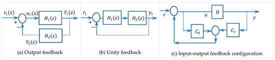
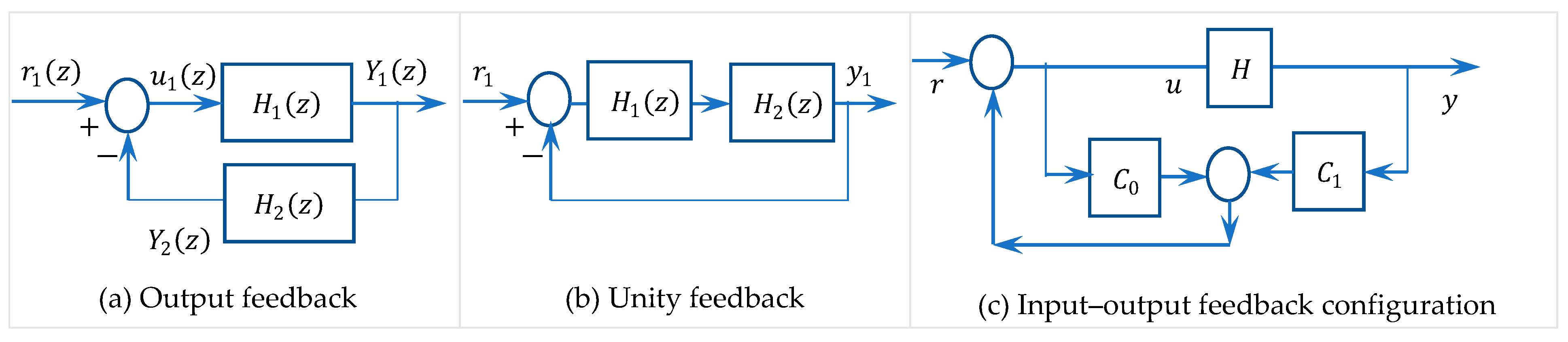
This section presents the design of dynamic compensator by block pole placement (i.e., full matrix polynomial assignment). By providing dynamic rather than static gains, such compensators offer greater design freedom and achieve objectives unattainable with static feedback, while keeping degree minimal. Common configurations (Figure 1) are unity feedback for sensitivity improvement, output feedback for tracking, and input–output feedback for unobservable states [22]. Using MFD, which generalize scalar rational functions to MIMO systems, the design builds a desired characteristic matrix polynomial from selected block poles and determines the compensator by solving the matrix Diophantine equation, with the minimal-degree-row solution meeting steady-state, transient, and pole-location requirements [6].

Figure 1. Various compensator structures for MFD of MIMO systems.

Theorem 12.

Let $H_1\left(z\right)\in {\mathbb{R}}^{p\times m}\left(z\right)$ and $H_2\left(z\right)\in {\mathbb{R}}^{m\times p}\left(z\right)$ be two rational matrix functions.

(1)

If $\det \left(I\pm H_1{H}_2\right)\ne 0$, then $H_1\left(z\right){\left[I\pm H_2\left(z\right)H_1\left(z\right)\right]}^{-1}={\left[I\pm H_1\left(z\right)H_2\left(z\right)\right]}^{-1}{H}_1\left(z\right)$；

(2)

The output feedback closed-loop transfer matrix $H_{\mathrm{c}\mathrm{l}\mathrm{s}}\left(z\right)=H_1\left(z\right){\left(I \pm H_2\left(z\right)H_1\left(z\right)\right)}^{-1}$ is proper if, and only if, $\left(I \pm H_2\left(\infty \right)H_1\left(\infty \right)\right)$ is nonsingular;

(3)

Moreover, if $H_1\left(z\right)\in {\mathbb{R}}^{p\times m}$ and $H_2\left(z\right)\in {\mathbb{R}}^{m\times p}$ are not necessarily proper, then we have $\det \left(I+H_2\left(z\right)H_1\left(z\right)\right)=\det \left(I+H_1\left(z\right)H_2\left(z\right)\right)$.

Proof. 

(1) The proof of the first part of the theorem is straight forward:

$$\begin{array}{c}\begin{array}{c}{\left[I \pm H_1\left(z\right)H_2\left(z\right)\right]}^{-1}{H}_1\left(z\right)=H_1\left(z\right){\left[I \pm H_2\left(z\right)H_1\left(z\right)\right]}^{-1}\\ ⬍\end{array}\\ \left[I \pm H_1\left(z\right)H_2\left(z\right)\right]H_1\left(z\right){\left[I \pm H_2\left(z\right)H_1\left(z\right)\right]}^{-1}=H_1\left(z\right)\end{array}$$

$$\mathrm{So} \left(I \pm H_1\left(z\right)H_2\left(z\right)\right)H_1\left(z\right)=H_1\left(z\right)\left(I \pm H_2\left(z\right)H_1\left(z\right)\right)$$

(2) Assume that we have negative output feedback configuration, as shown in Figure 1a, then $u_1\left(z\right)=r_1\left(z\right)-Y_2\left(z\right)$. For each sub-system we have, $Y_1\left(z\right)=H_1\left(z\right)u_1\left(z\right)$ and $Y_2\left(z\right)=H_2\left(z\right)Y_1\left(z\right)$, which means that $Y_1\left(z\right)=H_1\left[r_1-Y_2\right]=H_1\left(z\right)\left[r_1\left(z\right)-H_2\left(z\right)Y_1\left(z\right)\right]$. This implies that $\left[I+H_1\left(z\right)H_2\left(z\right)\right]Y_1\left(z\right)=H_1\left(z\right)r_1\left(z\right)$, and the overall transfer function is $H_{\mathrm{c}\mathrm{l}\mathrm{s}}\left(z\right)=H_1\left(z\right){\left(I+ H_2\left(z\right)H_1\left(z\right)\right)}^{-1}$; it is called proper (or causal) $\mathrm{i}\mathrm{f}$ $H_{\mathrm{c}\mathrm{l}\mathrm{s}}\left(\infty \right)=\mathrm{c}\mathrm{n}\mathrm{s}\mathrm{t}\ne \infty$. Now assume that $\underset{z\to \infty }{\lim }\left(I+ H_2\left(z\right)H_1\left(z\right)\right)=F$ and $\underset{z\to \infty }{\lim }{H}_1\left(z\right)=G$; furthermore, if $\det \left(F\right)\ne 0,$ then $\underset{z\to \infty }{\lim }{H}_{\mathrm{c}\mathrm{l}\mathrm{s}}\left(z\right)=G.F^{-1},$ or explicitly, $\underset{z\to \infty }{\lim }{H}_{\mathrm{c}\mathrm{l}\mathrm{s}}\left(z\right)=G.\mathrm{a}\mathrm{d}\mathrm{j}\left(F\right)/\det \left(F\right)$. Therefore, a necessary and sufficient condition for to be a proper rational function is the non-singularity of $F=\left(I+H_2\left(\infty \right)H_1\left(\infty \right)\right)$.

(3) Using the first part with the determinant, we obtain

$$\begin{array}{c} \\ \begin{array}{c} \\ \begin{array}{c}\det \left[H_1\left(z\right){\left[I \pm H_2\left(z\right)H_1\left(z\right)\right]}^{-1}\right]=\det \left[{\left[I \pm H_1\left(z\right)H_2\left(z\right)\right]}^{-1}{H}_1\left(z\right)\right]\\ \end{array}\end{array}\end{array}$$

This final result leads to $\det \left[I+H_2\left(z\right)H_1\left(z\right)\right]=\det \left[I+H_1\left(z\right)H_2\left(z\right)\right]$. □

Definition 13.

Consider a proper rational matrix transfer function $H\left(z\right)\in {\mathbb{R}}^{p\times m}$ factored as $H\left(z\right)=N_R\left(z\right)D_R^{-1}\left(z\right)=D_L^{-1}\left(z\right)N_L\left(z\right)$ . It is assumed that the matrix polynomials $D_R\left(z\right)$ and $N_R\left(z\right)$ are right coprime and $D_L\left(z\right)$ and $N_L\left(z\right)$ are left coprime; then, the characteristic polynomial of $H\left(z\right)$ is defined as $∆\left(z\right)=\mathit{det}\left(D_R\left(z\right)\right)=\mathit{det}\left(D_L\left(z\right)\right)$ and the degree of $H\left(z\right)$ is defined as $\mathit{deg}\left(H\left(z\right)\right)=\mathit{deg}\left[\mathit{det}\left(D_R\left(z\right)\right)\right] =\mathit{deg}\left[\mathit{det}\left(D_L\left(z\right)\right)\right],$ where $deg\left(.\right)$ and $det\left(.\right)$ stand for the degree and the determinant.

Definition 14.

A nonsingular $m^{th}$-order polynomial matrix $D\left(z\right)$ is said to be column-reduced if $\mathit{deg}\left[\mathit{det}\left(D\left(z\right)\right)\right]={⅀}_{i=1}^m{\delta }_{ci},$ where ${\delta }_{ci}$ is the maximum column degree, and it is said to be row-reduced if $\mathit{deg}\left[\mathit{det}\left(D\left(z\right)\right)\right]={⅀}_{i=1}^m{\delta }_{ri},$ where ${\delta }_{ri}$ is the maximum row degree of $D\left(z\right)$.

Column- and row-reduced polynomial matrices relate directly to the degree and properness of rational matrix functions, providing numerator–denominator degree bounds essential for properness [24]. The following lemma is key in compensator design, ensuring realizable controllers with minimal degree.

Lemma 4

([8]). If $D\left(z\right)$ is column-reduced, then $H\left(z\right)=N\left(z\right)D^{-1}\left(z\right)$ is strictly proper (proper) if, and only if, each column of $N\left(z\right)$ has a degree less than (less than or equal to) the degree of the corresponding column of $D\left(z\right)$.

3.1. Unity Feedback Compensators

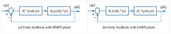
Many applied mathematicians have agreed on some arrangements and rules that facilitate mathematical work. Among these, we have to mention that in the field of control, if the matrix transfer function of the plant in the LMFD, then the controller should be designed in RMFD and vice versa (Figure 2 shows this illustration) [28,31].

Figure 2. Unity feedback configurations for MIMO systems described by RMFD and LMFD.

RMFD Plant: Consider the unity feedback system in Figure 2a. For a $p\times m$ system $H\left(z\right)=N_R\left(z\right)D_R^{-1}\left(z\right)$ described by a RMFD, the $m\times p$ compensator $C\left(z\right)$ will be described by a proper rational LMFD $C\left(z\right)=D_c^{-1}\left(z\right)N_c\left(z\right)$.

The closed-loop transfer matrix is given by $H_{\mathrm{c}\mathrm{l}\mathrm{s}}\left(z\right)= {\left[I_p+H\left(z\right)C\left(z\right)\right]}^{-1}H\left(z\right)C\left(z\right)$. Using the first part of Theorem 12, we obtain

$$H_{cls}\left(z\right)={\left(I_p+H\left(z\right)C\left(z\right)\right)}^{-1}H\left(z\right)C\left(z\right)=H\left(z\right){\left(I_m+C\left(z\right)H\left(z\right)\right)}^{-1}C\left(z\right)$$

Replacing $H\left(z\right)=N_R\left(z\right)D_R^{-1}\left(z\right)$ and $C\left(z\right)=D_c^{-1}\left(z\right)N_c\left(z\right)$ in $H_{\mathrm{c}\mathrm{l}\mathrm{s}}\left(z\right)$ yields

$$\begin{array}{c} \\ H_{cls}\left(z\right)=N_R\left(z\right){\left(D_c\left(z\right)D_R\left(z\right)+N_c\left(z\right)N_R\left(z\right)\right)}^{-1}{N}_c\left(z\right)\end{array}$$

Define the matrix polynomial $D_F\left(z\right)=D_c\left(z\right)D_R\left(z\right)+N_c\left(z\right)N_R\left(z\right);$ then, we have $H_{\mathrm{c}\mathrm{l}\mathrm{s}}\left(z\right)=N_R\left(z\right)D_F^{-1}\left(z\right)N_c\left(z\right)$. The design problem is, given $D_R\left(z\right)$, $N_R\left(z\right)$, and an arbitrary $D_F\left(z\right)$, determine $D_c\left(z\right)$ and $N_c\left(z\right),$ satisfying the closed-loop compensator equation $D_F=D_c{D}_R+N_c{N}_R$. The roots of $D_F\left(z\right)$ are the closed-loop poles, and its solvents are the block poles of $H_{\mathrm{c}\mathrm{l}\mathrm{s}}\left(z\right)$. Achieving arbitrary block pole placement for the feedback configurations described earlier requires solving the compensator matrix Diophantine equation, whose solvability was addressed in Theorem 11.

LMFD Plant: Consider the unity feedback system in Figure 2b. For a $p\times m$ system $H\left(z\right)=D_L^{-1}\left(z\right)N_L\left(z\right)$ described by a LMFD, the $m\times p$ compensator will be described by a proper rational RMFD $C\left(z\right)=N_c\left(z\right)D_c^{-1}\left(z\right)$. Following the same steps, we obtain

$$\begin{array}{c} \\ \begin{array}{c}\begin{array}{c}{H}_{cls}\left(z\right)={\left(I+D_L^{-1}\left(z\right)N_L\left(z\right)N_c\left(z\right)D_c^{-1}\left(z\right)\right)}^{-1}{D}_L^{-1}\left(z\right)N_L\left(z\right)N_c\left(z\right)D_c^{-1}\left(z\right)\\ =D_c\left(z\right){\left(D_L\left(z\right)D_c\left(z\right)+N_L\left(z\right)N_c\left(z\right)\right)}^{-1}{N}_L\left(z\right)N_c\left(z\right)D_c^{-1}\left(z\right)\end{array}\\ =D_c\left(z\right){\left[D_F\left(z\right)\right]}^{-1}{N}_L\left(z\right)N_c\left(z\right)D_c^{-1}\left(z\right) \end{array}\end{array}$$

where $D_F\left(z\right)=D_L\left(z\right)D_c\left(z\right)+N_L\left(z\right)N_c\left(z\right)$ is the “left” Diophantine equation. If we replace $N_L{N}_c=D_F-D_L{D}_c$ in $H_{\mathrm{c}\mathrm{l}\mathrm{s}}\left(z\right)$, we obtain $H_{\mathrm{c}\mathrm{l}\mathrm{s}}\left(z\right)= I-D_c\left(z\right){\left[D_F\left(z\right)\right]}^{-1}{D}_L\left(z\right)$. Like before, the poles of $D_F\left(z\right)$ are the poles of the closed-loop system, and the compensator is determined by solving the Diophantine equation.

To solve the matrix Diophantine equation, the functional form is converted into an equivalent algebraic form, known as the Sylvester matrix equation, which is more suitable for a computational solution [22,25]. 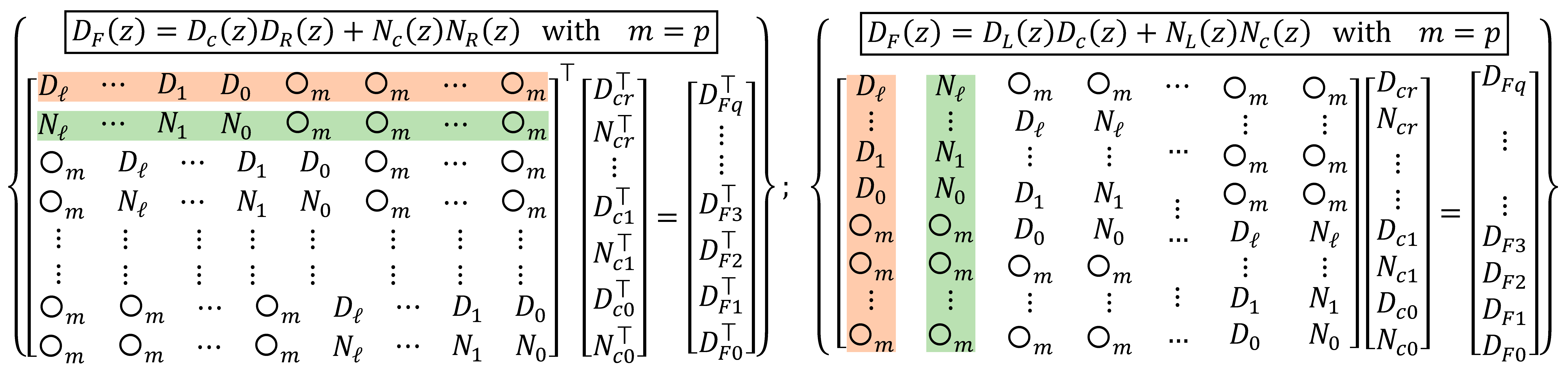If the subscript r stands for the degree of compensator and $\mathsf{\ell }$ is the degree of open loop transfer function $H\left(z\right)$, then the closed-loop degree is $q=\mathsf{\ell }+r$.

Remark. 

The existence of a MIMO controller using this procedure depends on the solvability of the last rectangular matrix equation [6].

3.2. Output Feedback Configuration

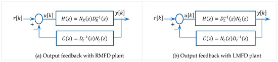
A dynamic compensator acts as an observer with linear feedback of the estimated state, producing dynamic output feedback. Since this affects only the controllable and observable part of the system, coprime MFDs are used to represent it [30]. This section introduces the output feedback configuration, as shown in Figure 3.

Figure 3. Output feedback configurations for MIMO systems described by RMFD-LMFDs.

RMFD Plant: For a system described in RMFD $H\left(z\right)=N_R\left(z\right)D_R^{-1}\left(z\right)$ and the compensator described in LMFD $C\left(z\right)=D_c^{-1}\left(z\right)N_c\left(z\right)$, the closed-loop transfer function of the configuration of Figure 3a is given by $H_{\mathrm{c}\mathrm{l}\mathrm{s}}\left(z\right) = H\left(z\right){\left[I + C\left(z\right)H\left(z\right)\right]}^{-1},$ where $H\left(z\right)$ and $C\left(z\right)$ have polynomial coefficients with the following dimensions: $D_{Ri}$, $D_{ci}\in {\mathbb{R}}^{m\times m}$, $N_{Ri}\in {\mathbb{R}}^{p\times m}$, and $N_{ci}\in {\mathbb{R}}^{m\times p}$. So, the closed-loop transfer function is

$$\begin{array}{c}{H}_{cls}\left(z\right)=N_R\left(z\right)D_R^{-1}\left(z\right){\left[I+D_c^{-1}\left(z\right)N_c\left(z\right)N_R\left(z\right)D_R^{-1}\left(z\right)\right]}^{-1}\\ =N_R\left(z\right){\left[D_c\left(z\right)D_R\left(z\right)+N_c\left(z\right)N_R\left(z\right)\right]}^{-1}{D}_c\left(z\right)\end{array}$$

If we let $D_F=D_c{D}_R+N_c{N}_R$ be the right Diophantine equation, then the closed-loop transfer function will be $H_{\mathrm{c}\mathrm{l}\mathrm{s}}\left(z\right)=N_R\left(z\right){\left[D_F\left(z\right)\right]}^{-1}{D}_c\left(z\right)$ and the poles of $D_F\left(z\right)$ are the poles of $H_{\mathrm{c}\mathrm{l}\mathrm{s}}\left(z\right)$, and the compensator is fully determined by solving $D_F=D_c{D}_R+N_c{N}_R$.

LMFD Plant: For a system described by LMFD $H\left(z\right)=D_L^{-1}\left(z\right)N_L\left(z\right)$, the compensator is described by a RMFD $C\left(z\right)=N_c\left(z\right)D_c^{-1}\left(z\right)$, and the closed-loop system of Figure 3b will be rewritten as $H_{\mathrm{c}\mathrm{l}\mathrm{s}}\left(z\right)= {\left[I +H\left(z\right)C\left(z\right)\right]}^{-1} H\left(z\right),$ where the matrix parameters $D_{Li}$, $D_{ci}$ are $p\times p$ real matrices, $N_{Li}$ are $p\times m$ real matrices, and $N_{ci}$ are $m\times p$ real matrices. So, the closed-loop transfer function is

$$\begin{array}{c}{H}_{cls}\left(z\right)={\left[I+D_L^{-1}\left(z\right)N_L\left(z\right)N_c\left(z\right)D_c^{-1}\left(z\right)\right]}^{-1}{D}_L^{-1}\left(z\right)N_L\left(z\right)\\ =D_c\left(z\right) {\left[D_L\left(z\right)D_c\left(z\right)+N_L\left(z\right)N_c\left(z\right)\right]}^{-1}{N}_L\left(z\right)\end{array}$$

Let $D_F\left(z\right)=\left[D_L\left(z\right)D_c\left(z\right)+N_L\left(z\right)N_c\left(z\right)\right]$ be the left Diophantine equation; then, $H_{\mathrm{c}\mathrm{l}\mathrm{s}}\left(z\right)=D_c\left(z\right) {\left[D_F\left(z\right)\right]}^{-1}{N}_L\left(z\right)$. The poles of the closed-loop system are fully defined by the poles of $D_F\left(z\right)$ and the compensator can be determined.

3.3. Input–Output Feedback Configuration

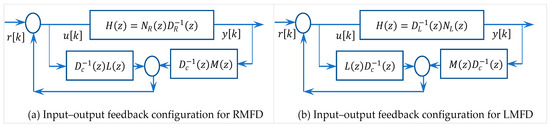
There are many possible two-DOF configurations. Here, a compensator is placed on the feedback path and another takes its inputs from the references (Figure 4); sometimes we call it two-parameter configuration or input–output feedback configuration (it seems to be more natural and more suitable for practical applications) [6,9].

Figure 4. Input–output (two-DOF) feedback configuration for MIMO systems.

RMFD Plant: Consider the input–output feedback system shown in Figure 4a. The plant is described by a $p\times m$ proper rational matrix $H\left(z\right)=N_R\left(z\right)D_R^{-1}\left(z\right)$. The compensators are denoted by the $m\times m$ proper rational matrix $C_0\left(z\right)=D_c^{-1}\left(z\right)L\left(z\right)$ and $m\times p$ rational matrix $C_1\left(z\right)=D_c^{-1}\left(z\right)M\left(z\right)$. The closed-loop transfer matrix can be computed as $H_{\mathrm{c}\mathrm{l}\mathrm{s}}\left(z\right)= H\left(z\right){\left[I +C_0\left(z\right)+C_1\left(z\right)H\left(z\right)\right]}^{-1}$. If we replace $H\left(z\right)$, $C_0\left(z\right)$ and $C_1\left(z\right)$ into $H_{\mathrm{c}\mathrm{l}\mathrm{s}}\left(z\right),$ then the closed-loop transfer function will be

$$\begin{array}{c} \\ \begin{array}{c} \\ \begin{array}{c}{H}_{cls}\left(z\right)=N_R\left(z\right)D_R^{-1}\left(z\right){\left[I+D_c^{-1}\left(z\right)L\left(z\right)+D_c^{-1}\left(z\right)M\left(z\right)N_R\left(z\right)D_R^{-1}\left(z\right)\right]}^{-1} \\ \end{array}\end{array}\end{array}$$

where $D_{Ri}$, $D_{ci},$ and $L_i$ are $m\times m$ real matrices, $N_{Ri}$ are $p\times m$ real matrices, and $N_{ci}$ are $m\times p$ real matrices and $M_i$ are $m\times p$ real matrices. An appropriate arrangement gives $H_{\mathrm{c}\mathrm{l}\mathrm{s}}\left(z\right)=N_R\left(z\right){\left[D_c\left(z\right)D_R\left(z\right)+L\left(z\right)D_R\left(z\right) +M\left(z\right)N_R\left(z\right)\right]}^{-1}{D}_c\left(z\right)$. Let us define the following matrix equation: $D_F\left(z\right)=D_c\left(z\right)D_R\left(z\right)+L\left(z\right)D_R\left(z\right) +M\left(z\right)N_R\left(z\right)$. The poles of the closed-loop system are fully defined by the poles of $D_F\left(z\right)$.

Let us define the error $E\left(z\right)=D_F\left(z\right)-D_c\left(z\right)D_R\left(z\right)=L\left(z\right)D_R\left(z\right)+M\left(z\right)N_R\left(z\right)$; then, the solution of the second part $L\left(z\right)D_R\left(z\right)+M\left(z\right)N_R\left(z\right)$ will determine the compensator numerators. If $D_c\left(z\right)$ and $D_F\left(z\right)$ are known, then the resolution of the Diophantine equation will determine the numerators of the two compensators $M\left(z\right)$ and $L\left(z\right)$. So, the closed-loop system will be $H_{\mathrm{c}\mathrm{l}\mathrm{s}}\left(z\right)=N_R\left(z\right){\left[D_F\left(z\right)\right]}^{-1}{D}_c\left(z\right)$.

LMFD Plant: Let us have the same feedback configuration as in Figure 4b. If $H\left(z\right)=D_L^{-1}\left(z\right)N_L\left(z\right)$ is in LMFD and the two compensators are in RMFD, $C_0\left(z\right)=L\left(z\right)D_c^{-1}\left(z\right)$ and $C_1\left(z\right)=M\left(z\right)D_c^{-1}\left(z\right)$. Then, the following development is obtained:

$$H_{cls}\left(z\right)=D_c\left(z\right){\left[D_L\left(z\right)D_c\left(z\right)+D_L\left(z\right)L\left(z\right)+N_L\left(z\right)M\left(z\right)\right]}^{-1}{N}_L\left(z\right)$$

Let us define $D_F\left(z\right)=D_L\left(z\right)D_c\left(z\right)+D_L\left(z\right)L\left(z\right)+N_L\left(z\right)M\left(z\right)$ as the desired closed-loop denominator and let $E\left(z\right)=D_F\left(z\right)-D_L\left(z\right)D_c\left(z\right)=D_L\left(z\right)L\left(z\right)+N_L\left(z\right)M\left(z\right)$. As before $H_{\mathrm{c}\mathrm{l}\mathrm{s}}\left(z\right)=D_c\left(z\right){\left[D_F\left(z\right)\right]}^{-1}{N}_L\left(z\right)$, the second part of the equation is the compensator equation, which can be solved if the compensator denominator is fixed arbitrarily.

Pre-compensators: Pre-compensators place zeros and reduce open-loop interactions in multivariable systems. While static designs are simple, dynamic pre-compensators often provide superior performance. Shamgah proposed a QP-based method to achieve diagonal dominance for decoupling, and Basilio designed a pre-compensator to minimize the eigenvector matrix condition number and improve normality for effective use of the characteristic locus method [6,21,22].

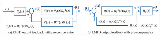
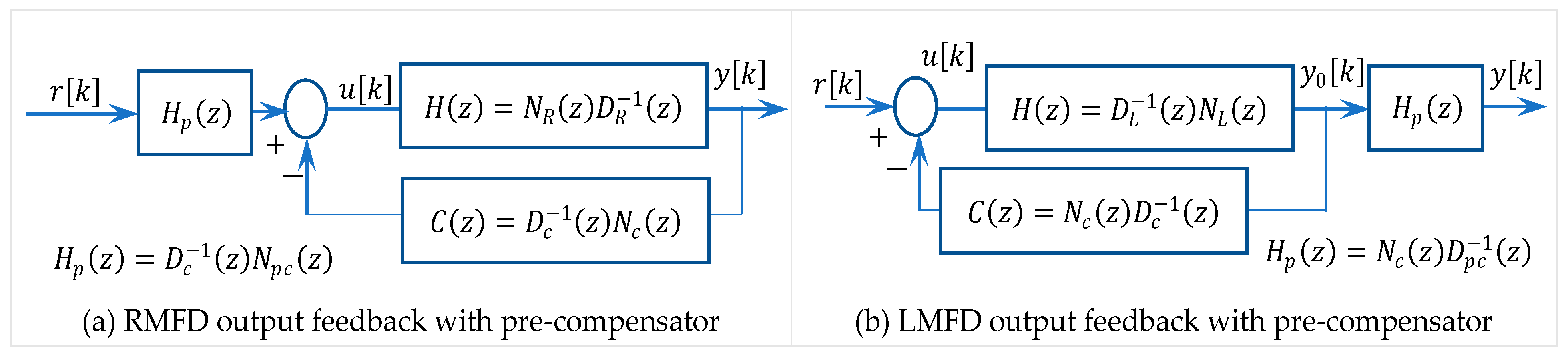
Figure 5 presents an example of a feedback configuration with a dynamic pre-compensator to place eventual desired zeros, where $H_p\left(z\right)$ is $m\times p$, $H\left(z\right)$ is $p\times m$, and $C\left(z\right)$ is $m\times p$. If $H\left(z\right)$ is in RMFD so $H_p\left(z\right)$ is in LMFD, then the closed-loop system will be as follows: $H_{\mathrm{c}\mathrm{l}\mathrm{s}}\left(z\right)=N_R\left(z\right){\left[D_F\left(z\right)\right]}^{-1}{D}_c\left(z\right)H_p\left(z\right)$, with $D_F\left(z\right)=D_c{D}_R+N_c{N}_R$. If $H\left(z\right)$ is in LMFD so $C\left(z\right)$ is in RMFD, then the closed-loop system will be as follows: $H_{\mathrm{c}\mathrm{l}\mathrm{s}}\left(z\right)=H_p\left(z\right)D_c\left(z\right){\left[D_F\left(z\right)\right]}^{-1}{N}_L\left(z\right)$, with $D_F\left(z\right)= D_L{D}_c +N_L{N}_c$.

Figure 5. Closed-loop denominator shaping via pre-compensator placement.

Remark. 

From the last obtained results, we conclude that the poles of $D_F\left(z\right)$are the poles of the closed-loop system and the zeros of the closed-loop system will be constituted by the zeros of the plant, the poles of the compensator denominator, and the zeros of the pre-compensator, which we can chose in order to achieve a certain goal.

Proposition 1.

From the desired block poles, we can construct the denominator of the closed-loop system. Given a set of $\mathsf{\ell }$ right desired block-roots $R_{di}\in {\mathbb{R}}^{m\times m}$ for $i=1,\dots ,\mathsf{\ell }$ , a right matrix polynomial $D_F\left(z\right)=I_m{s}^{\mathsf{\ell }}+{⅀}_{i=0}^{\mathsf{\ell }-1}{D}_{Fi}{z}^{\mathsf{\ell }-i}$ can be formed using the following relation: $\left[D_{F\mathsf{\ell }}\dots D_{F2} D_{F1}\right]=-\left[R_{d1}^{\mathsf{\ell }} R_{d2}^{\mathsf{\ell }}\dots R_{d\mathsf{\ell }}^{\mathsf{\ell }}\right].V_R^{-1}$ or equivalently $\left[D_{F\mathsf{\ell }}\dots D_{F1}\right]=-row{\left(R_{di}^{\mathsf{\ell }}\right)}_{i=1}^{\mathsf{\ell }}.V_R^{-1},$ where $V_R$ is the right-block Vandermonde matrix. Also, we can construct the $D_F\left(z\right)$ from a set of left solvents using the following equation: ${\left[D_{F\mathsf{\ell }}^{⟙}\dots D_{F1}^{⟙}\right]}^{⟙}=-V_L^{-1}.col{\left(L_{di}^{\mathsf{\ell }}\right)}_{i=1}^{\mathsf{\ell }},$ where $V_L$ is a left-block Vandermonde matrix, $V_L=col{\left[row{\left(L_{di}^{k-1}\right)}_{k=1}^{\mathsf{\ell }}\right]}_{i=1}^{\mathsf{\ell }}$.

4. Model-Approximation Theory and MIMO Identification Algorithms

System identification offers an approximate model often sufficient for control objectives. To this end, we review key MIMO identification algorithms in [1,2,4,12]. While conventional MIMO least squares (MLS) methods are widely used in literatures, their sensitivity to output noise motivates the use of two-step instrumental variable (IV) estimators based on auxiliary models [1]. Additional bias-reduction strategies include weighted least squares (WLS) using modulating functions and bias-compensated least squares (BCLS) with the GPMF approach [14]. For detailed insights into ARX model estimation techniques, see [4].

4.1. MIMO Least Squares

The least squares method can be seen as a data fitting method. It was developed by Gauss and first applied in celestial mechanics, e.g., to predict the future trajectory of the asteroid Ceres. The idea of the method is as follows. There is a number $N$ of equations involving a number $n$ of unknowns (or parameters) which are organized in the vector $\theta$. The least squares solution tries to minimize the error by minimizing the sum of squared errors. The method is especially elegant if the equations are linear in the parameters $\theta$. A MIMO ARMAX (autoregressive moving average with exogenous excitation) mode [3]

$$A\left(z^{-1}\right)y\left[k\right]=B\left(z^{-1}\right)u\left[k\right]+C\left(z^{-1}\right)e\left[k\right]; z^{-1} \mathrm{i}\mathrm{s} \mathrm{t}\mathrm{h}\mathrm{e} \mathrm{b}\mathrm{a}\mathrm{c}\mathrm{k}\mathrm{w}\mathrm{a}\mathrm{r}\mathrm{d} \mathrm{s}\mathrm{h}\mathrm{i}\mathrm{f}\mathrm{t} \mathrm{o}\mathrm{p}\mathrm{e}\mathrm{r}\mathrm{a}\mathrm{t}\mathrm{o}\mathrm{r}$$

(19)

This expression can alternatively be reformulated using the (LMFD) as

$$y\left[k\right]={\left(A\left(z^{-1}\right)\right)}^{-1}B\left(z^{-1}\right)u\left[k\right]+{\left(A\left(z^{-1}\right)\right)}^{-1}C\left(z^{-1}\right)e\left[k\right]$$

(20)

where $u\left[k\right]\in {\mathbb{R}}^m$ and $y\left[k\right]\in {\mathbb{R}}^p$ are input and output vectors of the system, respectively, while $e\left[k\right]\in {\mathbb{R}}^p$ is a white-noise signal and the polynomial matrices $A\left(z^{-1}\right),\hspace{0.17em}\hspace{0.17em}B\left(z^{-1}\right)$ and $C\left(z^{-1}\right)$ have the following structure: $A\left(z^{-1}\right) = I_p+A_1{z}^{-1}+A_2{z}^{-2}+...+A_{na}{z}^{-na}$, $B\left(z^{-1}\right)=B_1{z}^{-1}+...+B_{nb}{z}^{-nb}$ and $C\left(z^{-1}\right)=I_p+C_1{z}^{-1}+...+C_{nc}{z}^{-nc}$. The identification task focuses on estimating the matrix coefficients $A_i\in {\mathbb{R}}^{p\times p}$ and $B_i\in {\mathbb{R}}^{p\times m}$ that define the matrix polynomials $A\left(z^{-1}\right)$ and $B\left(z^{-1}\right)$, under the assumption that $C\left(z^{-1}\right)=I_p$, the identity matrix [4,12,13]. By transposing Equation (19) and the expansion of $A\left(z^{-1}\right)$ and $B\left(z^{-1}\right)$, we obtain the following expression $e^{⟙}\left[k\right]=y^{⟙}\left[k\right]-{\phi }^{⟙}\left[k\right]\theta$; that is

$$\begin{array}{c}{e}^{⟙}\left[k\right]= \left(y^{⟙}\left[k\right]+y^{⟙}[k-1]A_1^{⟙}+\cdots +y^{⟙}[k-na]A_{na}^{⟙}\right)-\left(u^{⟙}[k-1]B_1^{⟙}+\cdots +u^{⟙}[k-nb]B_{nb}^{⟙}\right)\\ \hspace{0.17em}\hspace{0.17em}\hspace{0.17em}= y^{⟙}\left[k\right]-\left[-y^{⟙}[k-1]\dots -y^{⟙}[k-n_a],u^{⟙}[k-1]\dots u^{⟙}[k-n_b]\right]{\left[A_1\dots A_{na},B_1\dots B_{nb}\right]}^{⟙}\end{array}$$

where the parameter matrix $\theta$ and the regression vector ${\phi }^{⟙}\left[k\right]$ are defined as $\theta ={\left[A_1\dots A_{na},\hspace{0.17em}{B}_1\dots B_{nb}\right]}^{⟙}$, ${\phi }^{⟙}\left[k\right]=\left[-y^{⟙}\left[k-1\right]\dots -y^{⟙}\left[k-n_a\right],u^{⟙}\left[k-1\right]\dots u^{⟙}\left[k-n_b\right]\right]$. So, the least squares estimate is

$${\hat{\theta }}_{ls}={\left({\varphi }^{⟙}\varphi \right)}^{-1}{\varphi }^{⟙}Y \mathrm{w}\mathrm{i}\mathrm{t}\mathrm{h} \varphi =\left[{\varphi }_y ⋮ {\varphi }_u\right]$$

(21)

$$Y=\left[\begin{array}{c}{y}^{⟙}[n+1,:]\\ ⋮\\ y^{⟙}[M,:]\end{array}\right]; {\varphi }_y=\left[\left[\begin{array}{c}-y^{⟙}\left[n,:\right]\\ ⋮\\ -y^{⟙}\left[M-1,:\right]\end{array}\right]\begin{array}{c}\cdots \\ \cdots \\ \cdots \end{array}\left[\begin{array}{c}-y^{⟙}\left[n-n_a+1,:\right]\\ ⋮\\ -y^{⟙}\left[M-n_a,:\right]\end{array}\right]\right];\hspace{0.17em}\hspace{0.17em} {\varphi }_u=\left[\left[\begin{array}{c}{u}^{⟙}\left[n,:\right]\\ ⋮\\ u^{⟙}\left[M-1,:\right]\end{array}\right]\begin{array}{c}\cdots \\ \cdots \\ \cdots \end{array}\left[\begin{array}{c}{u}^{⟙}\left[n-n_b+1,:\right]\\ ⋮\\ u^{⟙}\left[M-n_b,:\right]\end{array}\right]\right]$$

where $n=n_a$ and $M$ is the number of $I/O$ data. To avoid a large space memory and the large dimension matrix inversion taken by the simple least squares, a MIMO recursive least square algorithm can be handled and elaborated to be used in digital software preserving the memory space; see [1,2,3,4,17].

4.2. MIMO Recursive Least Squares

In the next subsection, we present our MIMO system-identification attempts using LMFD, with a recursive MIMO least squares implementation given as Algorithm 1:

Algorithm 1: Matrix Polynomial Recursive Least Squares
1	$\mathbf{A}-\mathrm{I}\mathrm{n}\mathrm{i}\mathrm{t}\mathrm{i}\mathrm{a}\mathrm{l}\mathrm{i}\mathrm{z}\mathrm{e}\hspace{0.17em}\theta \hspace{0.17em}\mathrm{t}\mathrm{o}\hspace{0.17em}\mathrm{z}\mathrm{e}\mathrm{r}\mathrm{o}\hspace{0.17em}\mathrm{a}\mathrm{n}\mathrm{d}\mathrm{l}\mathrm{e}\mathrm{t}\hspace{0.17em}\hspace{0.17em}P=c\times I\hspace{0.17em}\hspace{0.17em}\hspace{0.17em}\mathrm{W}\mathrm{h}\mathrm{e}\mathrm{r}\mathrm{e}\hspace{0.17em}\hspace{0.17em}c\hspace{0.17em}\hspace{0.17em}\mathrm{i}\mathrm{s}\hspace{0.17em}\mathrm{a}\hspace{0.17em}\mathrm{c}\mathrm{o}\mathrm{n}\mathrm{s}\mathrm{t}\mathrm{a}\mathrm{n}\mathrm{t}$
2	$\mathbf{B}-\mathrm{F}\mathrm{o}\mathrm{r}\hspace{0.17em}\hspace{0.17em}k=n_a\hspace{0.17em}:\hspace{0.17em}N-1$
3	$\hspace{1em}\psi ={\left[-y^{⟙}[k,:]...-y^{⟙}[k-n_a+1,:],u^{⟙}[k,:] ...u^{⟙}[k-n_b+1,:]\right]}^{⟙}$
4	$\hspace{1em}G=\left(P\psi \right){\left(1+{\psi }^{⟙}P\psi \right)}^{-1}\hspace{0.17em}$
5	$\hspace{1em}\theta =\theta +G\left(y^{⟙}\left[k+1,:\right]-{\psi }^{⟙}\theta \right)$
6	$\hspace{1em}P=\left(I-G{\psi }^{⟙}\right)P\hspace{0.17em}$
7	$\mathrm{E}\mathrm{n}\mathrm{d}$

Proof. 

In many practical cases, it is necessary that parameter estimation takes place concurrently with the system’s operation. This parameter estimation problem is called on-line identification and its methodology usually leads to a recursive procedure for every new measurement (or data entry). For this reason, it is also called recursive identification. In the previous sections we have seen that the ordinary least square is given by

$${\theta }_k={\left({\varphi }^{⟙}\varphi \right)}^{-1}{\varphi }^{⟙}Y={\left[{⅀}_{i=1}^k\psi \left(i\right){\psi }^{⟙}\left(i\right)\right]}^{-1}\left[{⅀}_{i=1}^k\psi \left(i\right)y^{⟙}\left(i\right)\right]$$

If we define $P_k={\left[{⅀}_{i=1}^k\psi \left(i\right){\psi }^{⟙}\left(i\right)\right]}^{-1}$, then we obtain ${\theta }_k=P_k.\left[{⅀}_{i=1}^k\psi \left(i\right)y\left(i\right)\right]$ and $P_{k+1}^{-1}={⅀}_{i=1}^{k+1}\psi \left(i\right){\psi }^{⟙}\left(i\right)=P_k^{-1}+\psi \left(k+1\right){\psi }^{⟙}\left(k+1\right);$ therefore,

$${\theta }_{k+1}=P_{k+1}\left[P_k^{-1}{\theta }_k+\psi \left(k+1\right)y^{⟙}\left(k+1\right)\right]=P_{k+1}{P}_k^{-1}{\theta }_k+P_{k+1}\psi \left(k+1\right)y^{⟙}\left(k+1\right)$$

or, equivalently, ${\theta }_{k+1}=P_{k+1}\left[P_{k+1}^{-1}-\psi \left(k+1\right){\psi }^{⟙}\left(k+1\right)\right]{\theta }_k+P_{k+1}\psi \left(k+1\right)y^{⟙}\left(k+1\right)$.

Now we can summarize this development into the following:

$$\left\{\begin{array}{l}{\theta }_{k+1}={\theta }_k+P_{k+1}\psi \left(k+1\right)\left[y^{⟙}\left(k+1\right)-{\psi }^{⟙}\left(k+1\right){\theta }_k\right]\\ P_{k+1}={\left[P_k^{-1}+\psi \left(k+1\right){\psi }^{⟙}\left(k+1\right)\right]}^{-1} \end{array}\right\}$$

To avoid matrix inversion, we use ${\left[A+BCD\right]}^{-1}=A^{-1}-A^{-1}B{\left[C^{-1}+D{A}^{-1}B\right]}^{-1}D{A}^{-1}$, and we define the change in variables $A=P_k^{-1}$, $B=\psi \left(k+1\right)$, $C=1$ and $D={\psi }^{⟙}\left(k+1\right)$; we obtain $P_{k+1}=P_k-P_k\psi \left(k+1\right){\psi }^{⟙}\left(k+1\right)P_k/\left[1+{\psi }^{⟙}\left(k+1\right)P_k\psi \left(k+1\right)\right]$. If we define the following $G=P_{k+1}\psi \left(k+1\right),$ and by using the previous result, we obtain

$$\begin{array}{c} \\ \begin{array}{c}G=P_{k+1}\psi \left(k+1\right)=P_k-{\displaystyle \frac{P_k\psi \left(k+1\right){\psi }^{⟙}\left(k+1\right)P_k\psi \left(k+1\right)}{1+{\psi }^{⟙}\left(k+1\right)P_k\psi \left(k+1\right)}}={\displaystyle \frac{P_k\psi \left(k+1\right)}{1+{\psi }^{⟙}\left(k+1\right)P_k\psi \left(k+1\right)}}\\ \end{array}\end{array}$$

In particular, applications errors occurring at different time instants may have varying importance. For instance, older errors are often considered less significant. To account for this, we introduce a weighted error vector, ${\epsilon }_W=W\epsilon =W\left(Y-\varphi \theta \right)$, where $W$ is a weighting matrix, typically chosen as diagonal. The associated weighted LS criterion is $\mathcal{J}\left(\epsilon \right)={\epsilon }_W^{⟙}{\epsilon }_W={\left(Y-\varphi \theta \right)}^{⟙}{W}^{⟙}W\left(Y-\varphi \theta \right)$. Minimizing $\mathcal{J}\left(\epsilon \right)$ with respect to $\theta$ yields $\theta ={\left[{\varphi }^{⟙}{W}^{⟙}W\varphi \right]}^{-1}{\varphi }^{⟙}{W}^{⟙}WY$. We denote $Q=W^{⟙}W=\mathrm{d}\mathrm{i}\mathrm{a}\mathrm{g}\left({\lambda }^{N-1},\dots ,\lambda ,{\lambda }^0\right)$, with $0.9<\lambda <0.99,$ and $\lambda$ is called the forgetting factor. The recursive version of this algorithm is $P_{k+1}={\lambda }^{-1}\left(P_k-P_k\psi \left(k+1\right){\psi }^{⟙}\left(k+1\right)P_k/\left[\lambda +{\psi }^{⟙}\left(k+1\right)P_k\psi \left(k+1\right)\right]\right)$.

A simulation experiment has been performed for signal-to-noise ratio equal to 20 db for both outputs; the next example shows the results. □

Example 1.

Consider the next dynamical system with the following matrices:

$$A\left(z^{-1}\right)=\left[\begin{array}{cc}1& 0\\ 0& 1\end{array}\right]+\left[\begin{array}{cc}0.5& -0.4\\ 0.3& -0.6\end{array}\right]z^{-1}+\left[\begin{array}{cc}-0.1& -0.3\\ 0.2& 0.3\end{array}\right]z^{-1}; B(z^{-1})=\hspace{0.17em}\left[\begin{array}{cc}-0.1& -0.9\\ 0.4& 0.5\end{array}\right]z^{-1}$$

A PRBS data sequence of length $N=1000$ is used to excite the system. A simulation experiment has been performed for signal to noise ratio equal to 20db for both outputs. The results of using the next algorithm is as follows:

$$⌊\begin{array}{c}\begin{array}{c}\begin{array}{l}P=1000\times I; \\ \mathrm{F}\mathrm{o}\mathrm{r}\hspace{0.17em}\hspace{0.17em}\hspace{0.17em}k=2\hspace{0.17em}:\hspace{0.17em}1000-1\hspace{0.17em}\hspace{0.17em}\mathrm{d}\mathrm{o},\end{array}\\ \hspace{1em}\hspace{1em}\hspace{1em}\psi ={\left[-y^{⟙}[k,:],-y^{⟙}[k-2+1,:],u^{⟙}[k,:]\right]}^{⟙},\hspace{1em}\hspace{1em} G=\left(P\psi \right){\left(1+{\psi }^{⟙}P\psi \right)}^{-1},\hspace{0.17em}\hspace{0.17em}\hspace{0.17em}\end{array}\hspace{0.17em}\\ \hspace{1em}\hspace{1em}\hspace{1em}\theta =\theta +G\left(y^{⟙}\left(k+1,:\right)-{\psi }^{⟙}\theta \right)\hspace{0.17em},\hspace{0.17em}\hspace{0.17em}\hspace{0.17em}\hspace{0.17em}\hspace{0.17em}\hspace{0.17em} \hspace{0.17em}\hspace{0.17em} \hspace{0.17em}\hspace{0.17em}\hspace{0.17em}P=\left(I-G{\psi }^T\right)P \end{array}$$

Which are given by

$${\theta }^{⟙}=\left[A_1 A_2 B_1\right]=\left[\begin{array}{cc}0.5015& -0.4006\\ 0.3047& -0.5953\end{array}\begin{array}{c} ⋮\\ ⋮\end{array} \begin{array}{cc}-0.0947& -0.2994\\ 0.2053& 0.6957\end{array}\begin{array}{c} ⋮\\ ⋮\end{array} \begin{array}{cc}-0.0992& -0.8998\\ 0.4027& 0.5021\end{array}\right]$$

where the dimension of the corresponding matrices are, respectively, $\dim \left(\psi \right)=6\times 1$, $\dim \left(G\right)=6\times 1$, $\dim \left(P\right)=6\times 6$, $\dim \left(\theta \right)=6\times 2,$ and $\dim \left(I\right)=6\times 6$.

Comments:

▪

The MIMO-RLS reduces the computation load associated with MIMO least squares by casting it in recursive form which is useful for online system identification;

▪

This basic RLS can be improved by introducing a forgetting factor [4] in order to give more weight to the most recent data.

4.3. MIMO Maximum Likelihood

For maximum likelihood (ML) method purpose, introduce the further assumption that the noise in the model (19) is Gaussian-distributed. The ML estimates of $\theta$ is obtained by maximizing the likelihood function, i.e., the probability distribution function (PDF) of the observations conditioned on the parameter vector $\theta$. For the previously given A MIMO ARMAX model, Equation (19) can be developed to yield [4,12,17]

$$\begin{array}{c} \\ \begin{array}{c} \\ \begin{array}{c}\begin{array}{c} \\ C\left(z^{-1}\right)e\left[k\right]= \left(y\left[k\right]+A_{1}y\left[k-1\right]+...+A_{n_a}y\left[k-n_a\right]\right)-\left(B_{1}u\left[k-1\right]+...+B_{n_b}u\left[k-n_b\right]\right)\end{array}\\ \end{array}\end{array}\end{array}$$

This equation can be rewritten using the Kronecker operator ($⨂$) as

$$e\left[k\right]=\left[I_p\otimes y^{⟙}\left[k\right]\right]\mathrm{c}\mathrm{o}\mathrm{l}\left(I_p\right)-\left[{\eta }_y,{\eta }_u,{\eta }_e\right]\theta$$

(22)

where

$$\begin{array}{l} \\ \begin{array}{l}\begin{array}{c}{\eta }_y=I_p\otimes y^{⟙}\left[k-1\right]+...+I_p\otimes y^{⟙}\left[k-n_a\right]\hspace{0.17em},\hspace{0.17em}\hspace{0.17em}{\eta }_u=-I_p\otimes u^{⟙}\left[k-1\right] ...-I_p\otimes u^{⟙}\left[k-n_b\right]\hspace{0.17em} \\ {\eta }_e=-I_p\otimes e^{⟙}\left[k-1\right]...-I_p\otimes e^{⟙}\left[k-n_c\right],\hspace{0.17em}\hspace{0.17em}\hspace{0.17em}\hspace{0.17em}\hspace{0.17em}\hspace{0.17em}\hspace{0.17em}\hspace{0.17em}\hspace{0.17em}\hspace{0.17em}\hspace{0.17em}\hspace{0.17em}\hspace{0.17em}\hspace{0.17em}\theta ={\left[{\theta }_A,{\theta }_B,{\theta }_C\right]}^{⟙}\hspace{0.17em}\hspace{0.17em} \\ {\theta }_A=\left[\mathrm{c}\mathrm{o}\mathrm{l}{\left(A_1^{⟙}\right)}^{⟙}...\mathrm{c}\mathrm{o}\mathrm{l}{\left(A_{n_a}^{⟙}\right)}^{⟙}\right],\hspace{0.17em}{\theta }_B=\left[\mathrm{c}\mathrm{o}\mathrm{l}{\left(B_1^{⟙}\right)}^{⟙}...\mathrm{c}\mathrm{o}\mathrm{l}{\left(B_{n_b}^{⟙}\right)}^{⟙}\right],\hspace{0.17em}{\theta }_C=\left[\mathrm{c}\mathrm{o}\mathrm{l}{\left(C_1^{⟙}\right)}^{⟙}...\mathrm{c}\mathrm{o}\mathrm{l}{\left(C_{n_c}^{⟙}\right)}^{⟙}\right]\end{array}\\ \end{array}\end{array}$$

The best estimate of the parameter $\hat{\theta }$ can be obtained using a numerical minimization algorithm, such as

$$\begin{array}{c}•\hspace{0.17em}\hspace{0.17em}\mathrm{Steepest}\hspace{0.17em}\hspace{0.17em}\mathrm{descent}\hspace{0.17em}\hspace{0.17em}\mathrm{method}:\hspace{0.17em}\hspace{0.17em}\hspace{0.17em}{\theta }_{k+1}={\theta }_k-\lambda {\nabla }^{⟙}E\\ •\hspace{0.17em}\hspace{0.17em}\mathrm{Gauss}\hspace{0.17em}\hspace{0.17em}\mathrm{Newton}\hspace{0.17em}\hspace{0.17em}\mathrm{method}:\hspace{0.17em}\hspace{0.17em}{\theta }_{k+1}={\theta }_k-{\nabla }^{⟙}{\nabla }^{⟙}E \end{array}$$

with

$$\nabla ={\left[{\left\{{\displaystyle \frac{\partial e[m+1]}{\partial {\theta }^{⟙}}}\right\}}^{⟙}\dots {\left\{{\displaystyle \frac{\partial e\left[N\right]}{\partial {\theta }^{⟙}}}\right\}}^{⟙}\right]}^{⟙}, \hspace{0.17em}\hspace{0.17em}\hspace{0.17em}\hspace{0.17em}\hspace{0.17em}\hspace{0.17em}\hspace{0.17em}\hspace{0.17em}\hspace{0.17em}\hspace{0.17em}\mathrm{and}\hspace{0.17em}\hspace{0.17em}\hspace{0.17em}\hspace{0.17em}\hspace{0.17em}\hspace{0.17em}\hspace{0.17em}\hspace{0.17em}\hspace{0.17em}\hspace{0.17em}\hspace{0.17em}\hspace{0.17em}\hspace{0.17em}E=\left[e^{⟙}\left[m+1\right]\cdots e^{⟙}\left[N\right]\right]$$

An implementation of the MIMO-ML can be written as Algorithm 2:

Algorithm 2: MIMO Maximum Likelihood (ML) Algorithm

1  Step 1: For $k=m+1\hspace{0.17em}\hspace{0.17em}\mathrm{t}\mathrm{o}\hspace{0.17em}\hspace{0.17em}N$

2   - Compute the prediction error $\widehat{e}\left[k\right]=\hat{A}\left(z^{-1}\right)y\left[k\right]-\hat{B}\left(z^{-1}\right)u\left[k\right]-C_1\hat{e}\left[k-1\right]...-C_{n_c}\hat{e}\left[k-n_c\right]$

3   - Compute the partial derivatives of $e\left[k\right]: \partial e\left[k\right]/\partial {\theta }^T$. Where its elements can be computed through MIMO

4   IIR (Infinite Impulse Response) digital filtering using the updated matrix coefficients estimates ${\hat{C}}_i$ of the

5   matrix 5polynomial $\hat{C}\left(z^{-1}\right)$.

6  Step 2: Estimate the parameter vector $\theta$ using

7      $\hspace{1em}•\hspace{0.17em}\hspace{0.17em}\mathrm{S}\mathrm{t}\mathrm{e}\mathrm{e}\mathrm{p}\mathrm{e}\mathrm{s}\mathrm{t}\hspace{0.17em}\hspace{0.17em}\mathrm{d}\mathrm{e}\mathrm{s}\mathrm{c}\mathrm{e}\mathrm{n}\mathrm{t}\hspace{0.17em}\hspace{0.17em}\mathrm{m}\mathrm{e}\mathrm{t}\mathrm{h}\mathrm{o}\mathrm{d}:\hspace{0.17em}\hspace{0.17em}\hspace{0.17em}{\theta }_{k+1}={\theta }_k-\lambda {\nabla }^{⟙}E$

8      $\hspace{1em}•\hspace{0.17em}\hspace{0.17em}\mathrm{G}\mathrm{a}\mathrm{u}\mathrm{s}\mathrm{s}-\mathrm{N}\mathrm{e}\mathrm{w}\mathrm{t}\mathrm{o}\mathrm{n}\hspace{0.17em}\hspace{0.17em}\mathrm{m}\mathrm{e}\mathrm{t}\mathrm{h}\mathrm{o}\mathrm{d}:\hspace{0.17em}\hspace{0.17em}{\theta }_{k+1}={\theta }_k-{\left({\nabla }^{⟙}\nabla \right)}^{-1}{\nabla }^{⟙}E$

9      $\hspace{1em}\mathrm{With}\hspace{0.17em}m=n_a, 0<\lambda <1\hspace{0.17em}\hspace{0.17em}\hspace{0.17em}\mathrm{and}\hspace{0.17em}\hspace{0.17em}\hspace{0.17em}N\hspace{0.17em}\mathrm{is}\hspace{0.17em}\mathrm{the}\hspace{0.17em}\mathrm{number}\hspace{0.17em}\mathrm{of}\hspace{0.17em}\hspace{0.17em}\mathrm{Input}/\mathrm{Output}\hspace{0.17em}\mathrm{data}.$

10   Step 3: If no convergence, go to step1.

Example 2.

Let us consider the 2-input 2-output process (i.e., $p=m=2$) described in LMFD by its polynomial matrices as

$$\begin{array}{c} \\ \begin{array}{c}\begin{array}{c}A\left(z^{-1}\right)=\left[\begin{array}{cc}1& 0\\ 0& 1\end{array}\right]+\left[\begin{array}{cc}0.5& -0.4\\ 0.3& -0.6\end{array}\right]z^{-1}+\left[\begin{array}{cc}-0.1& -0.3\\ 0.2& 0.3\end{array}\right]z^{-2}; B\left(z^{-1}\right)=\left[\begin{array}{cc}-0.1& -0.9\\ 0.2& 0.3\end{array}\right]z^{-1}+\left[\begin{array}{cc}-0.8& -0.3\\ 0.1& 0.7\end{array}\right]z^{-2}\\ \end{array}\\ C(z^{-1})=\left[\begin{array}{cc}1& 0\\ 0& 1\end{array}\right]+\left[\begin{array}{cc}0.7& 0.2\\ 0.3& -0.9\end{array}\right]z^{-1}+\left[\begin{array}{cc}0.3& 0.4\\ -0.5& 0.7\end{array}\right]z^{-2}\end{array}\end{array}$$

The aim is to estimate the matrix polynomials $A\left(z^{-1}\right)\hspace{0.17em},\hspace{0.17em}B\left(z^{-1}\right)$ and $C\left(z^{-1}\right) \hspace{0.17em}$ from I/O data contaminated by white noise. A PRBS data sequence of length $N=1000$ is used to excite the system. A simulation experiment has been performed for signal to noise ratio equal to 20 db for both outputs.

$$\left\{\begin{array}{c}\begin{array}{c}{\displaystyle \frac{\mathsf{\partial }e\left[k\right]}{\mathsf{\partial }\left({\theta }_A\right)}} = \left[{\displaystyle \frac{\mathsf{\partial }e\left[k\right]}{\mathsf{\partial }{\left(\mathrm{c}\mathrm{o}\mathrm{l}\right(A_1^{⟙}\left)\right)}^{⟙}}}, {\displaystyle \frac{\mathsf{\partial }e\left[k\right]}{\mathsf{\partial }{\left(\mathrm{c}\mathrm{o}\mathrm{l}\right(A_2^{⟙}\left)\right)}^{⟙}}}\right] = \left[C{\left(z^{-1}\right)}^{-1}\left[I_p\otimes y^{⟙}[k-1]\right],C{\left(z^{-1}\right)}^{-1}\left[I_p\otimes y^{⟙}[k-2]\right]\right] \\ {\displaystyle \frac{\mathsf{\partial }e\left[k\right]}{\mathsf{\partial }\left({\theta }_B\right)}} =\left[{\displaystyle \frac{\mathsf{\partial }e\left[k\right]}{\mathsf{\partial }{\left(\mathrm{c}\mathrm{o}\mathrm{l}\right(B_1^{⟙}\left)\right)}^{⟙}}}, {\displaystyle \frac{\mathsf{\partial }e\left[k\right]}{\mathsf{\partial }{\left(\mathrm{c}\mathrm{o}\mathrm{l}\right(B_2^{⟙}\left)\right)}^{⟙}}}\right] = -\left[C{\left(z^{-1}\right)}^{-1}\left[I_p\otimes u^{⟙}[k-1]\right],C{\left(z^{-1}\right)}^{-1}\left[I_p\otimes u^{⟙}[k-2]\right]\right]\end{array}\\ {\displaystyle \frac{\partial e\left[k\right]}{\mathsf{\partial }\left({\theta }_C\right)}} = \left[{\displaystyle \frac{\mathsf{\partial }e\left[k\right]}{\mathsf{\partial }{\left(\mathrm{c}\mathrm{o}\mathrm{l}\right(C_1^{⟙}\left)\right)}^{⟙}}}, {\displaystyle \frac{\mathsf{\partial }e\left[k\right]}{\mathsf{\partial }{\left(\mathrm{c}\mathrm{o}\mathrm{l}\right(C_2^{⟙}\left)\right)}^{⟙}}}\right] = -\left[C{\left(z^{-1}\right)}^{-1}\left[I_p\otimes e^{⟙}[k-1]\right],C{\left(z^{-1}\right)}^{-1}\left[I_p\otimes e^{⟙}[k-2]\right]\right] \end{array}\right\}$$

Finally, we can form$\mathsf{\partial }e\left[k\right]/\partial {\theta }^{⟙}=\left[\mathsf{\partial }e\left[k\right]/\mathsf{\partial }{\theta }_A, \mathsf{\partial }e\left[k\right]/\mathsf{\partial }{\theta }_B, \mathsf{\partial }e\left[k\right]/\mathsf{\partial }{\theta }_C\right],$ where its elements can be computed through MIMO IIR (Infinite Impulse Response) digital filtering using the updated matrix coefficients estimates ${\hat{C}}_1,\hspace{0.17em}{\hat{C}}_2$ of the matrix polynomial $\hat{C}\left(z^{-1}\right)=I_2+{\hat{C}}_1{z}^{-1}+{\hat{C}}_2{z}^{-2}$ Then, using the Gauss–Newton method to update the parameter vector $\theta$ gives the results shown below:

$$\begin{array}{l} \\ \begin{array}{l}\begin{array}{c}{\hat{\theta }}_A=\left[0.4932 -0.4055 0.2963 -0.6029 -0.1022 -0.2968 0.1975 0.3040\right]\\ {\hat{\theta }}_B=\left[-0.1056 -0.8996 0.1954 0.3014 -0.8017 -0.2929 0.1018 0.7053\right] \end{array}\\ {\hat{\theta }}_C=\left[0.7225 0.1946 0.3023 0.9205 0.3202 0.4200 -0.4972 0.7518\right] \end{array}\end{array}$$

Comments. 

The MIMO maximum likelihood algorithm is characterized by the use of the Kronecker product and block-structured filtering through MIMO IIR digital filters, which rely on continuously updated matrix coefficient estimates. The quality of system and noise dynamics estimation can be improved by increasing the number of data samples or by enhancing the signal-to-noise ratio [1,2,3].

5. The Proposed Adaptive Compensator Design

5.1. Conversion Between Left and Right Matrix Fraction Discerptions

A widely adopted approach for describing the input–output dynamics of MIMO systems is to express the transfer function as a ratio of matrix polynomials. This framework, known as the matrix fraction description, provides a concise representation of system behavior in the z-domain. For systems modeled by vector difference equations, the transfer matrices $H\left(z^{-1}\right)\hspace{0.17em}$ and $F\left(z^{-1}\right)\hspace{0.17em}$ can be arranged in rational polynomial form. Because matrix multiplication is generally non-commutative, two separate but equivalent forms are used: the left/right matrix fraction description (LMFD and RMFD), as explained in [26].

$$y\left[k\right]=H\left(z^{-1}\right)u\left[k\right]+F\left(z^{-1}\right)e\left[k\right]; z^{-1} \mathrm{i}\mathrm{s} \mathrm{t}\mathrm{h}\mathrm{e} \mathrm{b}\mathrm{a}\mathrm{c}\mathrm{k}\mathrm{w}\mathrm{a}\mathrm{r}\mathrm{d} \mathrm{s}\mathrm{h}\mathrm{i}\mathrm{f}\mathrm{t} \mathrm{o}\mathrm{p}\mathrm{e}\mathrm{r}\mathrm{a}\mathrm{t}\mathrm{o}\mathrm{r}$$

(23)

The transfer function matrix $H\left(z^{-1}\right)$ can be represented using two equivalent rational forms depending on the arrangement of the polynomial matrices:

$$\mathrm{R}\mathrm{M}\mathrm{F}\mathrm{D}: H\left(z^{-1}\right)=C\left(z^{-1}\right)D{\left(z^{-1}\right)}^{-1} \mathrm{o}\mathrm{r} \mathrm{L}\mathrm{M}\mathrm{F}\mathrm{D}: H\left(z^{-1}\right)=A{\left(z^{-1}\right)}^{-1}B\left(z^{-1}\right)$$

The matrix polynomials $A\left(z^{-1}\right)\hspace{0.17em},\hspace{0.17em}B\left(z^{-1}\right),C\left(z^{-1}\right)\hspace{0.17em}\hspace{0.17em}\mathrm{and}\hspace{0.17em}\hspace{0.17em}\hspace{0.17em}D\left(z^{-1}\right)$ involved in these expressions have the following general forms:

$$\begin{array}{c}A\left(z^{-1}\right)= I_p+A_1{z}^{-1}+...+A_{na}{z}^{-na},\hspace{0.17em}\hspace{0.17em}\hspace{0.17em}\hspace{0.17em}\hspace{0.17em}\hspace{0.17em}\hspace{0.17em}\hspace{0.17em}\hspace{0.17em}\hspace{0.17em}\hspace{0.17em}B\left(z^{-1}\right)= B_0+B_1{z}^{-1}+...+B_{nb}{z}^{-nb}.\\ C\left(z^{-1}\right)= C_0+C_1{z}^{-1}+...+C_{nc}{z}^{-nc},\hspace{1em}\hspace{1em}\hspace{0.17em}\hspace{0.17em}\hspace{0.17em}\hspace{0.17em}\hspace{0.17em}D\left(z^{-1}\right)= I_m+D_1{z}^{-1}+...+D_{nd}{z}^{-nd}.\end{array}$$

with the dimensions $A_i\in {\mathbb{R}}^{p\times p}, B_i\in {\mathbb{R}}^{p\times m}, C_i\in {\mathbb{R}}^{p\times m}\mathrm{and}{D}_i\in {\mathbb{R}}^{m\times m}$.

Remark 1.

It is possible to obtain either LMFD or RMFD from the other only by solving the following matrix equation:

$$A\left(z^{-1}\right)C\left(z^{-1}\right)=B\left(z^{-1}\right)D\left(z^{-1}\right)$$

(24)

This last matrix equality can be expanded and rewritten in more compact form after rearrangement into ${\mathbb{S}}_{AB}{\mathbb{S}}_{CD}={\mathbb{S}}_B$, where ${\mathbb{S}}_{AB}$  is the Silvester matrix

$$\begin{array}{c} \\ \begin{array}{c}{\mathbb{S}}_{AB}=\left[\begin{array}{cccccccccc}{I}_p& O_p& \cdots & O_p& O_p& O_{p\times m}& O_{p\times m}& \cdots & O_{p\times m}& O_{p\times m}\\ A_1& I_p& ⋮& ⋮& O_p& -B_1& O_{p\times m}& ⋮& ⋮& O_{p\times m}\\ ⋮& A_1& \ddots & I_p& ⋮& ⋮& -B_1& \ddots & O_{p\times m}& ⋮\\ A_{n_a}& ⋮& \ddots & A_1& I_p& -B_{n_b}& ⋮& \ddots & -B_1& O_{p\times m}\\ ⋮& A_{n_a}& ⋮& ⋮& A_1& ⋮& -B_{n_b}& ⋮& ⋮& -B_1\\ O_p& ⋮& \ddots & A_{n_a}& ⋮& O_{p\times m}& ⋮& \ddots & -B_{n_b}& ⋮\\ O_p& O_p& \cdots & O_p& A_{n_a}& O_{p\times m}& O_{p\times m}& \cdots & O_{p\times m}& -B_{n_b}\end{array}\right]; {\mathbb{S}}_{CD}=\left[\begin{array}{c}{C}_1\\ \begin{array}{c}{C}_2\\ \begin{array}{c}⋮\\ \begin{array}{c}{C}_{n_b}\\ \cdots \end{array}\end{array}\\ \begin{array}{c}\begin{array}{c}{D}_1\\ D_2\end{array}\\ ⋮\end{array}\end{array}\\ D_{n_a}\end{array}\right]; {\mathbb{S}}_B=\left[\begin{array}{c}{B}_1\\ \begin{array}{c}{B}_2\\ \begin{array}{c}⋮\\ \begin{array}{c}{B}_{n_b}\\ \cdots \end{array}\end{array}\\ \begin{array}{c}\begin{array}{c}{O}_{p\times m}\\ O_{p\times m}\end{array}\\ ⋮\end{array}\end{array}\\ O_{p\times m}\end{array}\right]\\ \end{array}\end{array}$$

and the solution vector is ${\mathbb{S}}_{CD}={\mathbb{S}}_{AB}^{+}{\mathbb{S}}_B,$ where ${\mathbb{S}}_{AB}^{+}={\left({\mathbb{S}}_{AB}^{⟙}{\mathbb{S}}_{AB}\right)}^{-1}{\mathbb{S}}_{AB}^{⟙}$

5.2. Non-Adaptive Compensator Design via the Linearly Independent Search Algorithm

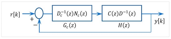
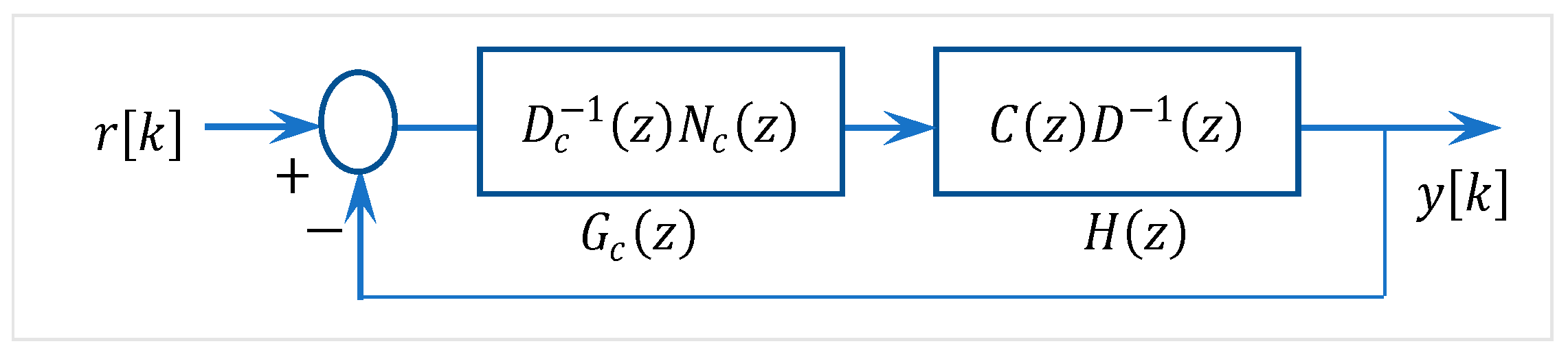
Now consider the unity feedback configuration shown in Figure 6. The plant is modeled as a proper rational matrix (in RMFD) of dimension $p\times m$, given by the transfer matrix $H\left(z^{-1}\right)=C\left(z^{-1}\right)D{\left(z^{-1}\right)}^{-1}$. The compensator is designed to be a proper rational matrix (in LMFD) of size $m\times p$, given by $G_c\left(z^{-1}\right)=D_c{\left(z^{-1}\right)}^{-1}{N}_c\left(z^{-1}\right)$.

Figure 6. Right matrix fraction descriptions (RMFD) compensator structure.

Accordingly, the resulting closed-loop transfer matrix is given by

$$H_{cl}\left(z^{-1}\right)={\left(I+H\left(z^{-1}\right)G_c\left(z^{-1}\right)\right)}^{-1}H\left(z^{-1}\right)G_c\left(z^{-1}\right)$$

(25)

Using the following matrix inverse identity, ${(I+AB)}^{-1}A=A{(I+BA)}^{-1},$ we obtain $H_{cl}\left(z^{-1}\right)=H\left(z^{-1}\right){\left[I+G_c\left(z^{-1}\right)H\left(z^{-1}\right)\right]}^{-1}{G}_c\left(z^{-1}\right)$ which can be written as

$$H_{cl}\left(z^{-1}\right)={\left(I+H\left(z^{-1}\right)G_c\left(z^{-1}\right)\right)}^{-1}H\left(z^{-1}\right)G_c\left(z^{-1}\right)$$

(26)

where $D_F\left(z^{-1}\right)$ is the Diophantine matrix equation and is defined by the next formula

$$D_F\left(z^{-1}\right)=D_c\left(z^{-1}\right)D\left(z^{-1}\right)+N_c\left(z^{-1}\right)C\left(z^{-1}\right)$$

(27)

Thus, the design objective can be reformulated as follows; given the matrices $D\left(z^{-1}\right)$ and $C\left(z^{-1}\right),$ along with a specified target matrix polynomial $D_F\left(z^{-1}\right)$, determine the compensator matrices $D_c\left(z^{-1}\right)$ and $N_c\left(z^{-1}\right)$ that fulfill the required relation. It is important to observe that the zeros of $D_F\left(z^{-1}\right)$ define the closed-loop system poles represented by $H_{cl}\left(z^{-1}\right)$, while the matrix solvents of $D_F\left(z^{-1}\right)$ represent the associated block poles of $H_{cl}\left(z^{-1}\right)$. In order to achieve a desired configuration of block poles for the unity feedback scheme presented earlier, one must solve the compensator matrix Equation (27). This process requires addressing a matrix Diophantine equation. Several numerical schemes have been introduced to tackle such problems, including the approaches referenced in [24,25]. The technique adopted in this section is based on the work of Chen [21]. The core idea is to convert the problem into a system of linear algebraic equations by constructing a Sylvester matrix (or, alternatively, a generalized resultant matrix) built from the matrix polynomials $\left\{B\left(z^{-1}\right) \mathrm{a}\mathrm{n}\mathrm{d} A\left(z^{-1}\right)\right\}$.

The Linearly Independent Search Algorithm: Given a sequence of n-dimensional row vectors $T_1,T_2,\dots ,T_p$, the proposed algorithm (Algorithm 3) constructs an $n\times n$ matrix $P\left(k\right)$ iteratively for each $k=\mathrm{1,2},\dots ,p$.

Algorithm 3: Linearly Independent Search Algorithm	Properties of this $P_k$:
1 $A.\hspace{0.17em}\hspace{0.17em}\hspace{0.17em}\mathrm{Initialize}\hspace{0.17em}P\left(0\right)=I_n\hspace{0.17em}\left(\hspace{0.17em}n\times n\hspace{0.17em}\hspace{0.17em}\mathrm{identity}\hspace{0.17em}\hspace{0.17em}\mathrm{matrix}\right)$
2 $B. \mathrm{For}\hspace{0.17em}k=\mathrm{1,2},...p\hspace{0.17em}\hspace{0.17em}\hspace{0.17em}\mathrm{do}$	▪ $P_k=P_k^2$.
3 $\mathrm{If}\hspace{0.17em}{T}_{k}P(k-1)T_k^{⟙}\ne 0\hspace{0.17em},\hspace{0.17em}\hspace{0.17em}\hspace{0.17em}\mathrm{Then}\hspace{0.17em}\hspace{0.17em}\hspace{0.17em}P(k)=P(k-1)\hspace{0.17em}-\hspace{0.17em}{\displaystyle \frac{\left[P\left(k-1\right)T_k^{⟙}\right]{\left[P\left(k-1\right)T_k^{⟙}\right]}^{⟙}}{T_{k}P(k-1)T_k^{⟙}}}$	▪ $P_k=P_k^{⟙}$.
4 $\mathrm{and}\hspace{0.17em}{T}_k\hspace{0.17em}\mathrm{is}\hspace{0.17em}\mathrm{linearly}\hspace{0.17em}\mathrm{independent}\hspace{0.17em}\mathrm{of}\hspace{0.17em}\mathrm{the}\hspace{0.17em}\mathrm{previous}\hspace{0.17em}\mathrm{rows}$	▪ $P_k\xi =\xi \forall \xi \perp \left\{T_1, T_2, \dots , T_k\right\}$.
5 $\mathrm{Else}\hspace{0.17em}\hspace{0.17em}P\left(k\right)=P\left(k-1\right)\hspace{0.17em}\hspace{0.17em}\hspace{0.17em}\mathrm{and}\hspace{0.17em}\hspace{0.17em}\hspace{0.17em}{T}_k\hspace{0.17em}\hspace{0.17em}\mathrm{is}\hspace{0.17em}\mathrm{linearly}\hspace{0.17em}\mathrm{dependent}.$	▪ $P_k{T}_i^{⟙}= 0 \forall T_i\in \left\{T_1, \dots , T_k\right\}$.

Proof. 

Given a real matrix $X\in {\mathbb{R}}^{m\times n}$ whose column vectors are the following, set $\mathcal{S}=\left\{x_1, x_2, \dots , x_n\right\}$. When the Gram–Schmidt algorithm is applied to the columns of $X$, the result is an orthogonal basis $\left\{u_1, u_2, \dots , u_n\right\}$ for the range space $\mathcal{R}\left(X\right)$, where

$$\begin{array}{c} \\ \begin{array}{c}{u}_k=x_k-{⅀}_{i=1}^{k-1}\left\{{\displaystyle \frac{⟨\left.u_i\right|x_k⟩}{⟨\left.u_i\right|x_i⟩}}{u}_i\right\}; P_{k-1}{x}_k=u_k where P_0=I and k=\mathrm{1,2}, \dots , n\\ \end{array}\end{array}$$

We will use the fact that

$${\displaystyle \frac{⟨\left.u_i\right|x_k⟩}{⟨\left.u_i\right|x_i⟩}}{u}_i={\displaystyle \frac{x_k^{⟙}{u}_i}{u_i^{⟙}{u}_i}}{u}_i=u_i{\displaystyle \frac{u_i^{⟙}{x}_k}{u_i^{⟙}{u}_i}}={\displaystyle \frac{u_i{u}_i^{⟙}}{u_i^{⟙}{u}_i}}{x}_k$$

Let us expand the $u_k$ formula and obtain the corresponding projecting matrix $P_k$, in terms of $x_k$ and the previous $P_{k-1}$.

We can prove the linearly independent search algorithm iteratively as follows:

$$⌊\begin{array}{l}\begin{array}{l}\begin{array}{l}\begin{array}{r}\mathbf{S}\mathbf{t}\mathbf{e}\mathbf{p} \mathbf{0}: P_0{x}_1=u_1 = x_1⟹ P_0= I\\ \mathbf{S}\mathbf{t}\mathbf{e}\mathbf{p} \mathbf{1}: P_1{x}_2=u_2 = x_2-{\displaystyle \frac{⟨\left.x_2\right|u_1⟩}{⟨\left.u_1\right|x_1⟩}}{u}_1=\left(I-{\displaystyle \frac{u_1{u}_1^{⟙}}{u_1^{⟙}{u}_1}}\right)x_2⟹ P_1=\left(P_0-{\displaystyle \frac{\left(P_0{x}_1\right){\left(P_0{x}_1\right)}^{⟙}}{{\left(P_0{x}_1\right)}^{⟙}\left(P_0{x}_1\right)}}\right)\end{array}\\ \begin{array}{l}\mathbf{S}\mathbf{t}\mathbf{e}\mathbf{p} \mathbf{2}: P_2{x}_3=u_3 = x_3-{\displaystyle \frac{⟨\left.x_3\right|u_1⟩}{⟨\left.u_1\right|x_1⟩}}{u}_1-{\displaystyle \frac{⟨\left.x_3\right|u_2⟩}{⟨\left.u_2\right|x_2⟩}}{u}_2=\left(I-{\displaystyle \frac{u_1{u}_1^{⟙}}{u_1^{⟙}{u}_1}}-{\displaystyle \frac{u_2{u}_2^{⟙}}{u_2^{⟙}{u}_2}}\right)x_3\\ \hspace{1em}\hspace{1em}\hspace{1em}\hspace{1em}\hspace{1em} =\left(P_0-{\displaystyle \frac{\left(P_0{x}_1\right){\left(P_0{x}_1\right)}^{⟙}}{{\left(P_0{x}_1\right)}^{⟙}\left(P_0{x}_1\right)}}-{\displaystyle \frac{\left(P_1{x}_2\right){\left(P_1{x}_2\right)}^{⟙}}{{\left(P_1{x}_2\right)}^{⟙}\left(P_1{x}_2\right)}}\right)x_3⟹ P_2=\left(P_1-{\displaystyle \frac{\left(P_1{x}_2\right){\left(P_1{x}_2\right)}^{⟙}}{{\left(P_1{x}_2\right)}^{⟙}\left(P_1{x}_2\right)}}\right)\end{array}\end{array}\\ \begin{array}{c}\\ \hspace{1em}\hspace{1em}\hspace{1em}\hspace{1em}\hspace{1em}\hspace{1em}\hspace{1em}\hspace{1em}\hspace{1em}\hspace{1em}\hspace{1em}\hspace{1em}\hspace{1em}\hspace{1em}\hspace{1em}\hspace{1em}\hspace{1em}⋮\end{array}\end{array}\\ \begin{array}{c}\\ \mathbf{S}\mathbf{t}\mathbf{e}\mathbf{p} \mathit{k}: P_k{x}_{k+1}=u_{k+1} = x_{k+1}-{⅀}_{i=1}^k\left\{{\displaystyle \frac{⟨\left.u_i\right|x_{k+1}⟩}{⟨\left.u_i\right|x_i⟩}}{u}_i\right\}=P_k=\left(P_{k-1}-{\displaystyle \frac{\left(P_{k-1}{x}_k\right){\left(P_{k-1}{x}_k\right)}^{⟙}}{{\left(P_{k-1}{x}_k\right)}^{⟙}\left(P_{k-1}{x}_k\right)}}\right)\end{array}\end{array}$$

Notice that, when $x_{k+1}$ is linearly dependent with the previous one, then $x_{k+1}=\beta x_k$ implies that $u_{k+1}=\beta u_k$, which can be written as $P_k{x}_{k+1}=\beta P_{k-1}{x}_k$ ⟺ $P_k=P_{k-1}$, and this will end the prove. □

5.3. Adaptation Mechanism Development

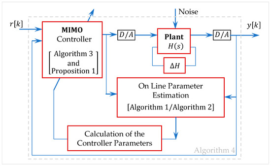
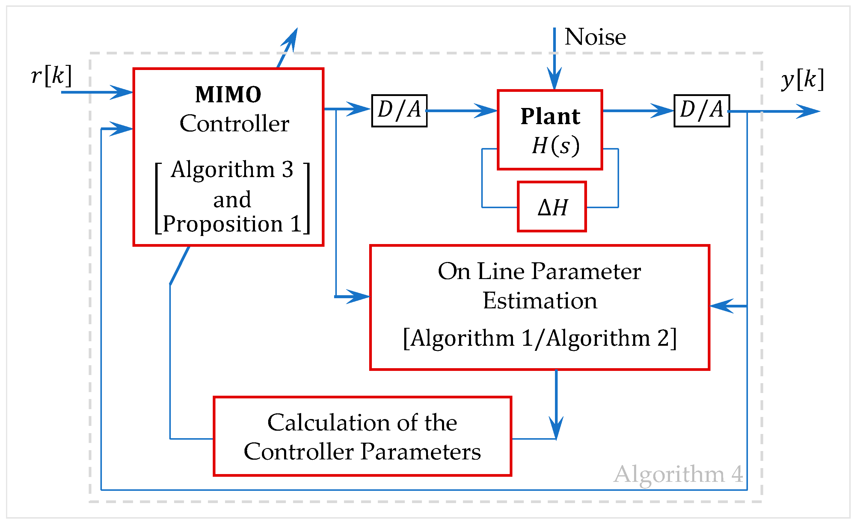
Classical controllers cannot effectively handle uncertainties in dynamic systems, as parameter variations alter operating conditions, leading to instability and degraded performance [47,48]. Adaptive control naturally addresses these issues by adjusting parameters to ensure closed-loop stability [15,23]. Two main types exist: model reference adaptive systems (MRAS) and self-tuning regulators (STRs). This work focuses on the self-tuning strategy, which relies on parametric estimation, as illustrated in Figure 7.

Figure 7. Indirect adaptive control structure (denominator shaping via block poles).

The novelty lies in the tight coupling between the Sylvester-based MFD transformation and the adaptive Diophantine solver, allowing exact block pole relocation under bounded parametric uncertainty (±7% in simulations) while retaining strict decoupling (<2% cross-channel influence). The proposed adaptive block pole placement scheme extends the matrix linear Diophantine equation framework into a fully online, eigenstructure-shaping control law for large-scale MIMO systems, as given in Algorithm 4.

Algorithm 4: The Adaptive Block-Pole Placement Algorithm
1	Step 1:	▪ Enter the values of: $M,n_a,n_b,\hspace{0.17em}\hspace{0.17em}P=c.I$
2		▪ Enter the nominal values of the $D_i\in {\mathbb{R}}^{m\times m}\hspace{0.17em}\hspace{0.17em}\hspace{0.17em}\mathrm{and}\hspace{0.17em}\hspace{0.17em}\hspace{0.17em}{C}_i\in {\mathbb{R}}^{p\times m}$
3		▪ Initiate by the values of $D_i\in {ℝ}^{m\times m}\hspace{0.17em}\hspace{0.17em}\mathrm{and}\hspace{0.17em}\hspace{0.17em}{C}_i\in {ℝ}^{p\times m}$
4		$\mathrm{For} \hspace{0.17em}k=n_a:M\hspace{0.17em} \mathrm{do}$
5	Step 2:	▪ Enter the desired Block poles $R_{id}\in {ℝ}^{m\times m}$ to be placed and construct the
6		$D_F\left(z^{-1}\right).$ Then compose: ${\hat{D}}_F\left(z^{-1}\right)={\hat{D}}_c\left(z^{-1}\right)\hat{D}\left(z^{-1}\right)+{\hat{N}}_c\left(z^{-1}\right)\hat{C}\left(z^{-1}\right)\hspace{0.17em}$.
7		▪ Solve the Diophantine equation using recursive search algorithm
8		▪ Obtain ${\hat{D}}_c\left(z^{-1}\right)$ and ${\hat{N}}_c\left(z^{-1}\right)$
9	Step 3:	▪ Give the desired trajectory sequence $r\left[k\right]$.
10		▪ Compute the closed-loop output and the control law by:
11		▪ $\begin{array}{c}y\left[k\right]=\hat{C}\left(z^{-1}\right)\hspace{0.17em}{\left({\hat{D}}_c\left(z^{-1}\right)\hspace{0.17em}\hat{D}\left(z^{-1}\right)\hspace{0.17em}+{\hat{N}}_c\left(z^{-1}\right)\hspace{0.17em}\hat{C}\left(z^{-1}\right)\hspace{0.17em}\right)}^{-1}{\hat{N}}_c\left(z^{-1}\right)\hspace{0.17em}r\left[k\right]\end{array}$
12		▪ $\begin{array}{c}u\left[k\right]={\hat{D}}_c\left(z^{-1}\right){\hat{N}}_c\left(z^{-1}\right)\hspace{0.17em}{u}_c\left[k\right]\hspace{0.17em}\mathrm{and} u_c\left[k\right]=r\left[k\right]-y\left[k\right]\end{array}$
13	Step 4:	Identify the plant parameters using: MIMO-RLS or MIMO-ML algorithms
14	Step 5:	Updating the matrix coefficients ${\theta }_{AB}={\hat{\theta }}_{AB}$. Convert LMFD to RMFD using
15		Silvester Matrix equation ${\hat{\theta }}_{CD}=\mathrm{funct}\left(A\left(z^{-1}\right),B\left(z^{-1}\right)\right)=\mathrm{funct}\left({\theta }_{AB}\right)$
16		▪ $\text{Getting} {\hat{C}}_i\in {ℝ}^{p\times m} \text{and} {\hat{D}}_i\in {ℝ}^{m\times m} \text{and} \text{go} \text{to} \text{Step}:2$

The proposed method guarantees the following criteria as summarized in Table 1:

Table 1. Performance guarantees of the proposed adaptive block pole placement method.

✓ Eigenvalue convergence:	$\underset{i}{\max }‖{\lambda }_i\left(D_F\left(z\right)\right)-{\lambda }_i\left({∆}_{\mathrm{c}\mathrm{l}\mathrm{o}\mathrm{s}\mathrm{e}\mathrm{d}}\left(z\right)\right)‖\le {10}^{-3}$
✓ Bounded tracking error:	$\underset{k\to \infty }{\lim }\mathrm{s}\mathrm{u}\mathrm{p}{‖e\left(k\right)‖}_{\infty }\le 0.02$
✓ Stability preservation:	All poles remain $\left|{\lambda }_i\right|<1$ during adaptation.

Sensitivity and Robustness Analysis: 

This adaptive mechanism merges high-precision block pole placement with online parametric learning, producing a compensator synthesis procedure that is both structurally minimal and robust to noise and disturbances, as validated in the winding process application. For a closed-loop system with transfer matrix $H_{\mathrm{c}\mathrm{l}\mathrm{s}}\left(z^{-1}\right)=N_R{\left[D_{c}D+N_{c}C\right]}^{-1}{D}_c,$ the sensitivity and complementary sensitivity functions are given, respectively, by $S\left(z^{-1}\right)={\left[I + H\left(z^{-1}\right)G_c\left(z^{-1}\right)\right]}^{-1}$ and $T\left(z^{-1}\right)=I-S\left(z^{-1}\right)=H\left(z^{-1}\right)G_c\left(z^{-1}\right){\left[I+H\left(z^{-1}\right)G_c\left(z^{-1}\right)\right]}^{-1}$. The robustness condition, with respect to multiplicative plant perturbations $H_{\Delta }\left(z^{-1}\right),$ satisfies ${‖T\left(z^{-1}\right)H_{\Delta }\left(z^{-1}\right)‖}_{\infty }<1$ which, in the polynomial domain, imposes a generalized eigenvalue bound

$$\rho \left(T\left(e^{j\omega }\right)H_{\Delta }\left(e^{j\omega }\right)\right)<1, \forall \omega \in [0,\pi ],$$

(28)

where $\rho \left(\cdot \right)$ denotes the spectral radius. For additive plant perturbation, the small-gain robust-stability test changes from involving $T$ to involving $M\left(z^{-1}\right)=G_c\left(z^{-1}\right)S\left(z^{-1}\right)$. The robust stability is guaranteed if ${‖G_c\left(z^{-1}\right)S\left(z^{-1}\right)H_{\Delta }\left(z^{-1}\right)‖}_{\infty }<1$ equivalently, on the unit circle $z=e^{j\omega }$ with $\omega \in [0,\pi ]$,

$$\mu \left(H_{cls},H_{\Delta }\right)=\underset{\omega \in [0,\pi ]}{\sup }{‖G_c\left(e^{j\omega }\right)S\left(e^{j\omega }\right)H_{\Delta }\left(e^{j\omega }\right)‖}_{\infty }<1$$

(29)

The block pole placement directly shapes the denominator $D_F\left(e^{j\omega }\right)$, allowing targeted reduction in the $H_{\infty }$-norm of $S\left(e^{j\omega }\right)$ in selected frequency ranges, thereby enhancing disturbance rejection while preserving robustness margins. Sensitivity minimization can be formalized as

$$\underset{D_c,N_c}{\min }{‖W_1\left(e^{j\omega }\right)S\left(e^{j\omega }\right)‖}_{\infty }$$

(30)

Subject to the Diophantine constraint $D_F=D_{c}D+N_{c}C,$ where $W_1\left(e^{j\omega }\right)$ is a frequency-weighting matrix enforcing robustness–performance trade-offs.

6. Application to Winding Process

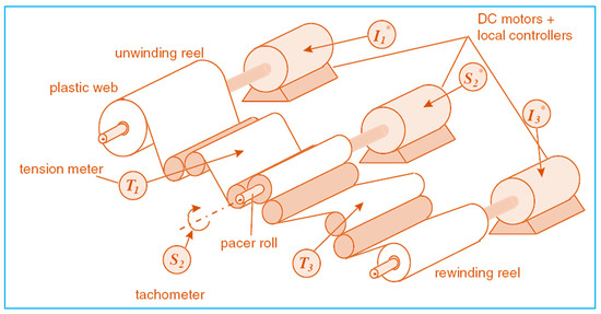
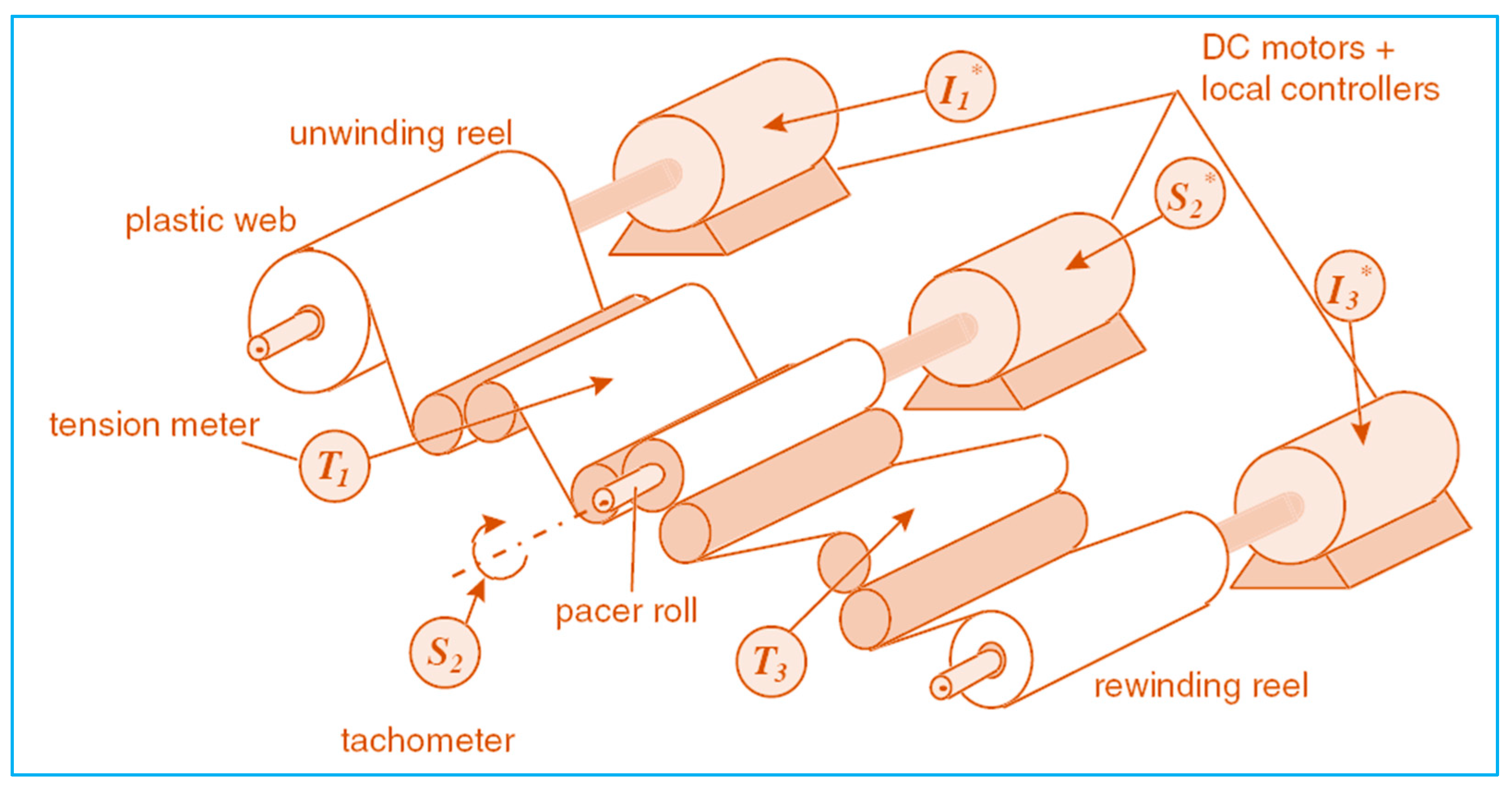
Winding systems are prevalent in many industrial sectors, including steel rolling mills and web-processing lines for coating, paper production, and polymer film extrusion. Their main purpose is to regulate web movement to reduce friction, slippage, and deformation, which can affect product quality [14]. The considered winding process (Figure 8) is modeled by $\dot{x}\left(t\right)=Ax\left(t\right)+Bu\left(t\right)$, $y\left(t\right)=Cx\left(t\right)$ and its variables are; $x\left(t\right)={\left[x_1 \dots x_6\right]}^{⟙}$ is the state vector, $u\left(t\right)={\left[u_1 u_2 u_3\right]}^{⟙}$ is the input vector, $y\left(t\right)={\left[y_1 y_2 y_3\right]}^{⟙}$ is the output vector. The constants $A\in {\mathbb{R}}^{6\times 6}$, $B\in {\mathbb{R}}^{6\times 3}$, and $C\in {\mathbb{R}}^{3\times 6}$ are the state-space matrices. The physical variables of the input/output vectors are as follows; $u_1$ is the setpoint of motor current 1, $u_2$ is the setpoint of motor angular speed 2, $u_3$ is the setpoint of motor current 3, $y_1$ is the web tension ($T_1$) between motors 1 and 2, $y_2$ is the web tension ($T_3$) between motors 2 and 3, and $y_3$ is the motor angular speed 2 (${\Omega }_2$).

Figure 8. Winding process showing sequential layering and alignment in prototype assembly.

The state-space model is derived directly from the linearized model of the winding process, as reported in earlier studies [3,14] and adopted in this work for validation.

$$\left\{ \begin{array}{c}A=\left[\begin{array}{cc}\begin{array}{ccc}\begin{array}{c}\begin{array}{c}-5.7174\\ 0.6513\\ 4.6614\end{array}\\ \begin{array}{c}-2.2842\\ 3.2578\\ 4.2846\end{array}\end{array} & \begin{array}{c}\begin{array}{c} 4.88430\\ -3.80000\\ -12.5805\end{array}\\ \begin{array}{c}-0.47720\\ -10.3059\\ -11.2052\end{array}\end{array} & \begin{array}{c}\begin{array}{c} 6.1395\\ 0.8200\\ -1.3596\end{array}\\ \begin{array}{c} 3.2639\\ -1.4336\\ -1.4066\end{array}\end{array}\end{array} & \begin{array}{ccc}\begin{array}{c}\begin{array}{c} 9.0408\\ 1.1555\\ -3.0943\end{array}\\ \begin{array}{c} 5.5751\\ -1.7843\\ -2.1079\end{array}\end{array} & \begin{array}{c}\begin{array}{c}-1.7346\\ -0.5212\\ -0.5536\end{array}\\ \begin{array}{c}-0.7958\\ 0.2381\\ -0.2192\end{array}\end{array} & \begin{array}{c}\begin{array}{c}-9.98310\\ 1.80720\\ 10.7326\end{array}\\ \begin{array}{c}-3.8630\\ 8.38510\\ 9.18760\end{array}\end{array}\end{array}\end{array}\right] \\ B=\left[\begin{array}{cc}\begin{array}{cc}\begin{array}{c}\begin{array}{c}0.043798\\ 0.105739\\ 0.358248\end{array}\\ \begin{array}{c}0.296437\\ 0.932283\\ 0.465714\end{array}\end{array}& \begin{array}{c}\begin{array}{c}0.956172\\ 0.235368\\ 0.154883\end{array}\\ \begin{array}{c}0.967756\\ 0.525201\\ 0.257882\end{array}\end{array}\end{array}& \begin{array}{c}\begin{array}{c}0.312443\\ 0.199597\\ 0.663932\end{array}\\ \begin{array}{c}0.667207\\ 0.266742\\ 0.515036\end{array}\end{array}\end{array}\right]; C^{⟙}=\left[\begin{array}{ccc}\begin{array}{c}\begin{array}{c}-0.027168\\ 0.075248\\ -0.010228\end{array}\\ \begin{array}{c} 0.019091\\ 0.026645\\ -0.062940\end{array}\end{array}& \begin{array}{c}\begin{array}{c} 0.610518\\ -0.714339\\ -0.275497\end{array}\\ \begin{array}{c}-0.601226\\ 0.025436\\ 0.792073\end{array}\end{array}& \begin{array}{c}\begin{array}{c}-0.164078\\ 0.300634\\ 0.049733\end{array}\\ \begin{array}{c} 0.163163\\ 0.066043\\ -0.325489\end{array}\end{array}\end{array}\right]\end{array} \right\}$$

Its corresponding RMFD model is given by $y\left[k\right]=C\left(z^{-1}\right)D{\left(z^{-1}\right)}^{-1}u\left[k\right],$ where $D\left(z^{-1}\right)=I_3+D_1{z}^{-1}+D_2{z}^{-2}$; $C\left(z^{-1}\right)=C_1{z}^{-1}+C_2{z}^{-2}$ and $I_3$ is the 3-by-3 identity matrix and the other matrix coefficients are

$$\left\{\begin{array}{l}\begin{array}{l}{D}_1=\left[\begin{array}{ccc}-2.2783& -0.06775& 0.55208\\ 1.8518& -1.66390& -2.95250\\ -1.1294& -0.17974& -0.18159\end{array}\right]\hspace{0.17em}, D_2=\left[\begin{array}{ccc} 1.2801& 0.067705& -0.55350\\ -1.8033& 0.672180& 2.87540\\ 1.0791& 0.171930& -0.73911\end{array}\right] \\ \end{array}\\ \begin{array}{c} \\ C_1=\left[\begin{array}{ccc}0.00429090& 0.0063885& -0.0128310\\ 0.06687700& 0.0087380& -0.1211500\\ 0.00077228& 0.0302260& 0.00060105\end{array}\right], C_2=\left[\begin{array}{ccc} 0.010399& -0.0027112& -0.015017\\ -0.144110& -0.0208320& 0.242840\\ 0.048767& -0.0216820& -0.079244\end{array}\right]\end{array}\end{array}\right\}$$

Remark. 

For simplify the control procedure we chose a first-order fixed-structure compensator $u\left[k\right]=\left[\hspace{0.17em}{\left[{\widehat{D}}_{c0}+{\widehat{D}}_{c1}{z}^{-1}\right]}^{-1}\left({\widehat{N}}_{c0}+{\widehat{N}}_{c1}{z}^{-1}\right)\right]\left(r\left[k\right]-y\left[k\right]\right)$with a constant gain pre-compensator $F=\hspace{0.17em}\underset{z\to 1}{\mathrm{l}\mathrm{i}\mathrm{m}}{\left[\widehat{C}\left(z^{-1}\right)D_F{\left(z^{-1}\right)}^{-1}{\widehat{N}}_c\left(z^{-1}\right)\right]}^{-1};$  then, the desired $D_F\left(z^{-1}\right)$  is a matrix polynomial of order three. Let us now chose thee block roots to be placed:

$$\begin{array}{c} \\ \begin{array}{c} \\ \left\{\begin{array}{c}\begin{array}{c}\begin{array}{c}\begin{array}{c}{R}_1=\left[\begin{array}{ccc}0.0000& -0.0082& 0.0033\\ 0.0306& -0.0533& 0.0228\\ 0.0028& -0.0041& -0.0045\end{array}\right]; \hspace{0.17em} \hspace{0.17em}{R}_2=\left[\begin{array}{ccc}0.0607& -0.0201& -0.0278\\ 0.1411& -0.0482& -0.0718\\ 0.0875& -0.0267& -0.0432\end{array}\right]; \hspace{0.17em}\hspace{0.17em}\hspace{0.17em}{R}_3=\left[\begin{array}{ccc}0.0499& -0.0223& -0.0250\\ 0.0156& -0.0023& -0.0133\\ 0.0572& -0.0285& -0.0302\end{array}\right]\end{array}\end{array}\\ \end{array}\\ {\sigma }_1\left(R_1\right)=\left\{-0.046;-0.0053;-0.0065\right\}; {\sigma }_2\left(R_2\right)=\left\{-0.033;0.0074;-0.0051\right\}; {\sigma }_3\left(R_3\right)=\left\{0.0054;-0.010;0.022\right\} \end{array}\right\}\end{array}\end{array}$$

where ${\sigma }_1\left(R_1\right), {\sigma }_2\left(R_2\right),$ and ${\sigma }_3\left(R_3\right)$  are the spectrum of those block roots. Hence, to reconstruct the desired matrix polynomial, we direct the reader to refer to [6,7]. Solving the Diophantine matrix equation $D_F\left(z^{-1}\right)=I_3+D_{F1}{z}^{-1}+D_{F2}{z}^{-2}+D_{F3}{z}^{-3}$ yield to the linear system of equations:

$$\begin{array}{c} \\ \left[\begin{array}{c}{\widehat{D}}_{c0}^{⟙}\\ {\widehat{D}}_{c1}^{⟙}\\ {\widehat{N}}_{c0}^{⟙}\\ {\widehat{N}}_{c1}^{⟙}\end{array}\right]=\left[{\left[\left[\begin{array}{cccc}{I}_3^{⟙}& D_1^{⟙}& D_2^{⟙}& {⭘}_3^{⟙}\\ {⭘}_3^{⟙}& I_3^T& D_1^{⟙}& D_2^{⟙}\\ {⭘}_3^{⟙}& C_1^{⟙}& C_2^{⟙}& {⭘}_3^{⟙}\\ {⭘}_3^{⟙}& {⭘}_3^{⟙}& C_1^{⟙}& C_2^{⟙}\end{array}\right]\left[\begin{array}{cccc}{I}_3^{⟙}& {⭘}_3^{⟙}& {⭘}_3^{⟙}& {⭘}_3^{⟙}\\ D_1^{⟙}& I_3^T& C_1^{⟙}& {⭘}_3^{⟙}\\ D_2^{⟙}& D_1^{⟙}& C_2^{⟙}& C_1^{⟙}\\ {⭘}_3^{⟙}& D_2^{⟙}& {⭘}_3^{⟙}& C_2^{⟙}\end{array}\right]\right]}^{-1}\left[\begin{array}{cccc}{I}_3^{⟙}& D_1^{⟙}& D_2^{⟙}& {⭘}_3^{⟙}\\ {⭘}_3^{⟙}& I_3^T& D_1^{⟙}& D_2^{⟙}\\ {⭘}_3^{⟙}& C_1^{⟙}& C_2^{⟙}& {⭘}_3^{⟙}\\ {⭘}_3^{⟙}& {⭘}_3^{⟙}& C_1^{⟙}& C_2^{⟙}\end{array}\right]\right]\left[\begin{array}{c}{I}_3^{⟙}\\ D_{F1}^{⟙}\\ D_{F2}^{⟙}\\ D_{F3}^{⟙}\end{array}\right]\end{array}$$

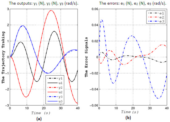
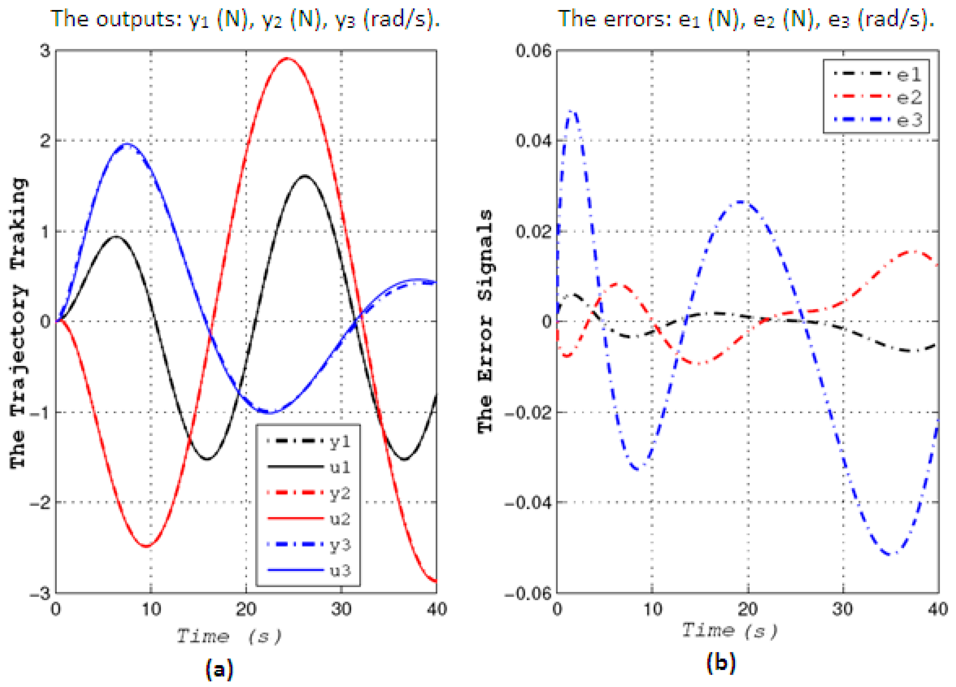
Nominal compensator coefficients are obtained from this equation. Assuming that the system uncertainties are of 7% of the nominal one means that the transfer function is $H\left(z^{-1}\right)=H_0\left(z^{-1}\right)+\Delta H\left(z^{-1}\right)$. Now, starting the adaptive block pole placement algorithm, we obtain the next results, as shown in Figure 9.

Figure 9. Adaptive trajectory tracking control. Sub-figure (a) denotes the responses of the tracking problem. Sub-figure (b) represents the dynamic error signals.

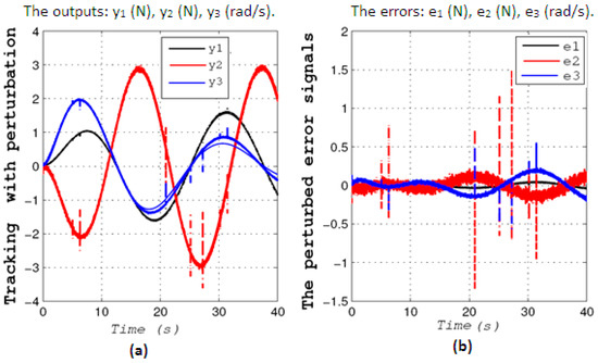
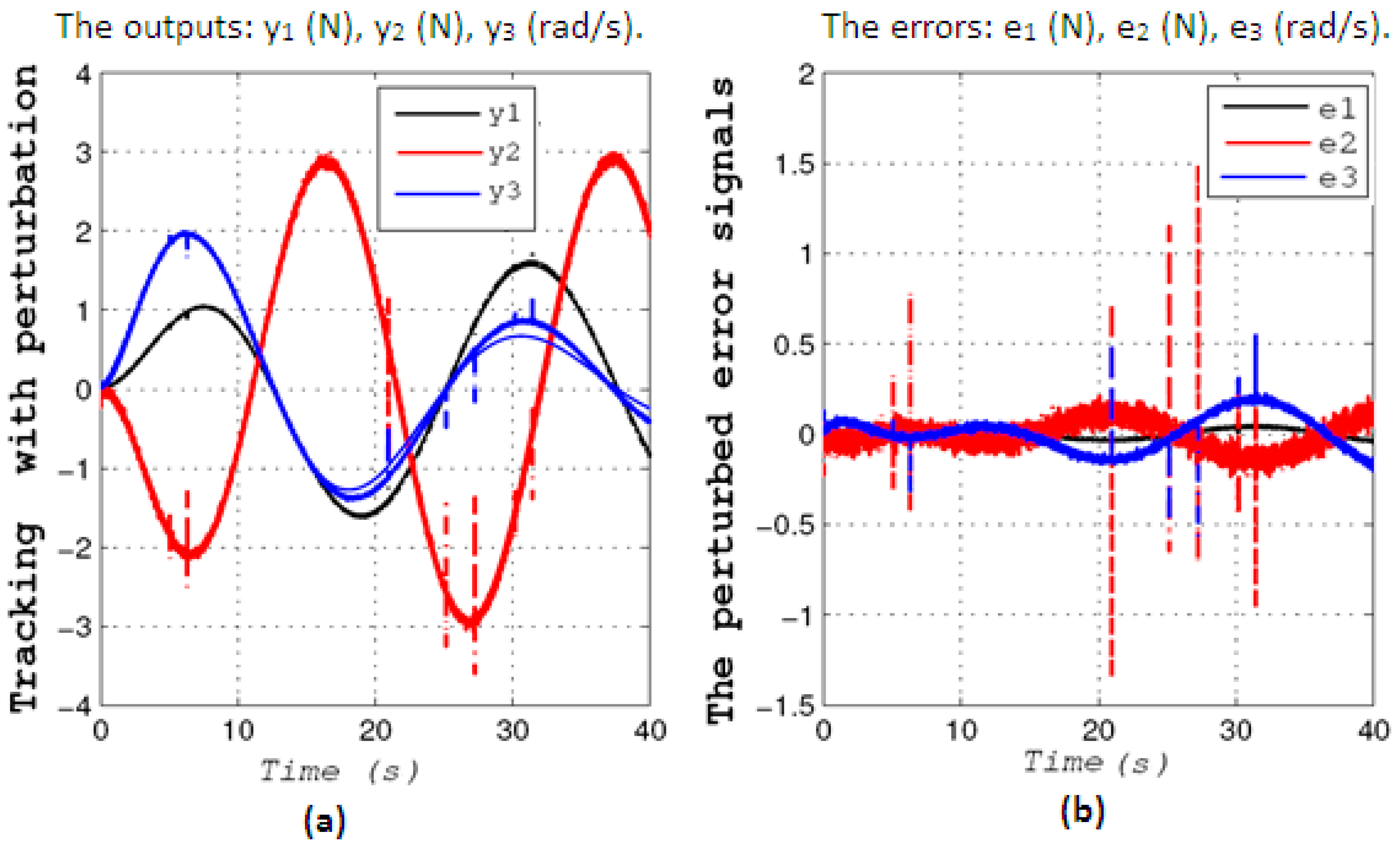
The simulation results (Figure 9) clearly indicate that the proposed algorithm successfully performs block pole placement, ensuring system stability even in the presence of abrupt parameter uncertainties, while maintaining low tracking errors. Specifically, Figure 9a shows that the system achieved block root assignment accuracy better than ±0.001, a mean steady-state error of less than 0.02, and maximum transient response time of 0.8 s under load variation. The effect of parameter variations had minimal impact on the performance of the digital compensator, which highlights the effectiveness of the adaptation mechanism. Moreover, Figure 9b shows that when the reference value of one control variable changes, the resulting interactions within the closed-loop system remain negligible, with cross-variable influence reduced to less than 2%. This implies that the system operates in a fully decoupled manner. Such decoupling is achieved because the MFD-based control structure generates coordinated actions across all control inputs as soon as any reference input changes. To evaluate the system’s capability for disturbance rejection, input pulses with amplitudes equal to one-tenth of the maximum input level were introduced, as illustrated in Figure 10. Additionally, white noise was injected at the system output to simulate measurement disturbances. Despite these perturbations, the system maintained robust regulation under 10% amplitude noise and step disturbances, effectively suppressing both transient and noise effects (see Figure 10a). Although some abrupt deviations appear in the output (see Figure 10b) due to the disturbances, the response quickly returns to its nominal state, demonstrating fast and reliable adaptive regulation.

Figure 10. Digital adaptive block pole assignment with perturbation rejection. Sub-figure (a) denotes the trajectory tracking. Sub-figure (b) represents the dynamic error signals.

To assess the robustness of the closed-loop transfer function, we compute the following:

• The smallest and the largest singular values

$${\sigma }_m\left(H_{cls}\right)=\underset{\omega \in \left[0 \pi \right]}{\mathrm{s}\mathrm{u}\mathrm{p}}\left[\sqrt{\left|{\lambda }_{min}\left({\Gamma }_{H_{cls}}\left(e^{j\omega }\right)\right)\right|}\right]; {\sigma }_M\left(H_{cls}\right)=\underset{\omega \in \left[0 \pi \right]}{\mathrm{s}\mathrm{u}\mathrm{p}}\left[\sqrt{\left|{\lambda }_{max}\left({\Gamma }_{H_{cls}}\left(e^{j\omega }\right)\right)\right|}\right]$$

where is the ${\mathsf{\Gamma }}_{H_{\mathrm{c}\mathrm{l}\mathrm{s}}}\left(e^{j\omega }\right)$ Gram matrix: ${\mathsf{\Gamma }}_{H_{\mathrm{c}\mathrm{l}\mathrm{s}}}\left(e^{j\omega }\right)=H_{\mathrm{c}\mathrm{l}\mathrm{s}}^{\mathrm{H}}\left(e^{j\omega }\right)H\left(e^{j\omega }\right)$;

2.

The condition number of the closed-loop transfer function

$$\chi \left(H_{cls}\left(e^{j\omega }\right)\right)={\sigma }_M\left(H_{cls}\right)/{\sigma }_m\left(H_{cls}\right);$$

3.

The infinity norm of the sensitivity function

$${‖S\left(e^{j\omega }\right)‖}_{\infty }=\underset{\omega \in \left[0 \pi \right]}{\mathrm{s}\mathrm{u}\mathrm{p}}\left[\sqrt{\left|{\lambda }_{max}\left(S_{cls}^H\left(e^{j\omega }\right)S\left(e^{j\omega }\right)\right)\right|}\right]$$

where $S\left(e^{j\omega }\right)={\left[I+H\left(e^{j\omega }\right)G_c\left(e^{j\omega }\right)\right]}^{-1}$.

Table 2 presents the robustness comparison using the extremal singular values, condition number, and $H_{\infty }$ norms of the closed-loop and sensitivity functions. The adaptive block pole/Diophantine design achieves the best conditioning and smallest sensitivity peaks, consistent with the simulation results on the $3\times 3$ winding process.

Table 2. Comparative robustness metrics (discrete time, evaluated on $e^{j\omega },\omega \in [0,\pi ]$).

	Method of [30]	Method of [39]	Method of [47]	The Proposed Method
${\sigma }_m\left(H_{cls}\right)$	0.28	0.40	0.52	0.62
${\sigma }_M\left(H_{cls}\right)$	2.90	2.10	1.80	1.35
$\chi \left(H_{cls}\left(e^{j\omega }\right)\right)$	10.4	5.3	3.5	2.2
${‖S\left(e^{j\omega }\right)‖}_{\infty }$	3.10	2.20	1.90	1.40
$\mu \left(H_{cls},H_{\Delta }\right)$	0.95	0.84	0.73	0.41

The adaptive block pole/Diophantine design achieves the largest minimum singular value and the smallest $\chi \left(H_{\mathrm{c}\mathrm{l}\mathrm{s}}\right)$, ensuring a well-conditioned closed loop with reduced modeling sensitivity. Its ${‖H_{\mathrm{c}\mathrm{l}\mathrm{s}}‖}_{\infty }$ remains close to unity, reflecting tight transient control, while the lowest ${‖S‖}_{\infty }$ (≈1.15) confirms robust stability against multiplicative uncertainty and effective disturbance rejection, consistent with fast regulation, low steady-state error, and minimal cross-channel interaction. In contrast, classical schemes show larger $\chi \left(H_{\mathrm{c}\mathrm{l}\mathrm{s}}\right)$ and sensitivity peaks, underscoring their vulnerability to noise and bias in MIMO settings. The method of [47] improves robustness compared to traditional schemes but still falls short of the adaptive block pole/Diophantine approach, whose explicit denominator shaping and online parameter adaptation provide clear performance advantages.

7. Conclusions

This study proposed and validated a new adaptive digital control technique based on matrix Diophantine equations for block pole placement in large-scale MIMO systems. The controller integrates recursive MIMO RLS identification with an adaptive compensator to achieve precise eigenstructure assignment even under significant parametric uncertainty (up to 7%). The numerical simulations on a three-input/three-output industrial winding process demonstrated excellent tracking performance, low interaction, and robust rejection of disturbances and sensor noise.

Specifically, the system achieved the following:

• Block root assignment accuracy better than ±0.001;
• Mean steady-state error of less than 0.02;
• Maximum transient response time of 0.8 s under load variation;
• Robust regulation under 10% amplitude noise and step disturbances;
• Complete decoupling, with cross-variable influence reduced to <2%.

While the validation has been limited to simulations, the selected case study and disturbance scenarios were designed to closely reflect industrial practice. The promising results suggest that the proposed strategy holds potential for real-world deployment in multivariable systems requiring fast and reliable online adaptation. Future work will focus on experimental implementation and comparative testing on industrial platforms to further confirm the practical viability of the approach.

References

- Mohamed, A. An Optimal Instrumental Variable Identification Approach for Left Matrix Fraction Description Models. Stud. Inform. Control. 2008, 17, 361–372. [Google Scholar]
- Akroum, M.; Hariche, K. Extending the SRIV Identification Algorithm to MIMO LMFD Models. J. Electr. Eng. Technol. 2009, 4, 135–142. [Google Scholar] [CrossRef] [Scilit]
- Mu, B.-Q.; Chen, H.-F.; Wang, L.Y.; Yin, G. Characterization and Identification of Matrix Fraction Descriptions for LTI Systems. SIAM J. Control. Optim. 2014, 52, 3694–3721. [Google Scholar] [CrossRef] [Scilit]
- Ljung, L. System Identification: Theory for the User; Prentice Hall: Englewood Cliffs, NJ, USA, 1999. [Google Scholar]
- Malika, Y.; Clark, T. A Contribution to the Polynomial Eigen Problem. Int. J. Math. Comput. Nat. Phys. Eng. 2014, 8, 1131–1338. [Google Scholar] [CrossRef]
- Yaici, M.; Hariche, K. On eigenstructure assignment using block poles placement. Eur. J. Control. 2014, 20, 217–226. [Google Scholar] [CrossRef] [Scilit]
- Cohen, N. Spectral analysis of regular matrix polynomials. Integral Equations Oper. Theory 1983, 6, 161–183. [Google Scholar] [CrossRef] [Scilit]
- DiStefano, J.J.; Stubberud, A.R. Theory and Problems of Feedback and Control Systems; Mc. Graw Hill: New York, NY, USA, 1967. [Google Scholar]
- Kamel, H. Interpolation Theory in the Structural Analysis of λ-matrices. Ph. D. Thesis, Cullen College of Engineering, University of Houston, Houston, TX, USA, 1987. [Google Scholar]
- Singla, S.; Tronsgard, A. Interpolation Polynomials and Linear Algebra. C. R. Math. Rep. Acad. Sci. Canada 2022, 44, 33–49. [Google Scholar]
- Hariche, K.; Denman, E.D. On Solvents and Lagrange Interpolating-Matrices. Appl. Math. Comput. 1988, 25, 321–332. [Google Scholar] [CrossRef] [Scilit]
- Zhu, Y.; Backx, T. Identification of Multivariable Industrial Processes; Springer-Verlag: London, UK, 1993. [Google Scholar]
- Al-Muthairi, N.; Bingulac, S.; Zribi, M. Identification of discrete-time MIMO systems using a class of observable canonical-form. Iee Proc. Control. Theory Appl. 2002, 149, 125–130. [Google Scholar] [CrossRef] [Scilit]
- Bastogne, T.; Noura, H.; Sibille, P.; Richard, A. Multivariable identification of a winding process by subspace methods for tension control. Control. Eng. Pr. 1998, 6, 1077–1088. [Google Scholar] [CrossRef] [Scilit]
- Landau, I.D.; Lozano, R.; Mohammed, M.; Karimi, A. Adaptive Control: Algorithms, Analysis and Applications; Springer-Verlag: London, UK, 2011. [Google Scholar]
- Pereira, E. On solvents of matrix polynomials. Appl. Numer. Math. 2003, 47, 197–208. [Google Scholar] [CrossRef] [Scilit]
- Ljung, L. Theory and Practice of Recursive Identification; MIT press: Cambridge, MA, USA; London, UK, 1987. [Google Scholar]
- Ahn, S. Stability of a matrix polynomial in discrete systems. IEEE Trans. Autom. Control. 1982, 27, 1122–1124. [Google Scholar] [CrossRef] [Scilit]
- Moore, B. On the flexibility offered by state feedback in multivariable systems beyond closed loop eigenvalue assignment. IEEE Trans. Autom. Control. 1976, 21, 689–692. [Google Scholar] [CrossRef] [Scilit]
- Wonham, W. On pole assignment in multi-input controllable linear systems. IEEE Trans. Autom. Control. 1967, 12, 660–665. [Google Scholar] [CrossRef] [Scilit]
- Chen, C.T. Linear System Theory and Design; Holt, Reinhart and Winston: New York, NY, USA, 1984. [Google Scholar]
- Kucera, V. Discrete Linear Control: The Polynomial Equation Approach; John Wiley: Hoboken, NJ, USA, 1979. [Google Scholar]
- Ioannou Petros, A. Robust Adaptive Control: Design, Analysis and Robustness Bounds; PTR Prentice-Hall: Upper Saddle River, NJ, USA, 1996. [Google Scholar]
- Fang, C.-H. A simple approach to solving the Diophantine equation. IEEE Trans. Autom. Control. 1992, 37, 152–155. [Google Scholar] [CrossRef] [Scilit]
- Fan, C.H.; Chang, F.R. A novel approach for solving Diophantine equations. IEEE Trans. Circuits Syst. 1990, 37, 1455–1457. [Google Scholar] [CrossRef] [Scilit]
- Bekhiti, B. The Left and Right Block Pole Placement Comparison Study: Application to Flight Dynamics. Inform. Eng. Int. J. (IEIJ) 2016, 4, 41–62. [Google Scholar] [CrossRef]
- Zaitsev, V. On arbitrary matrix coefficient assignment for the characteristic matrix polynomial of block matrix linear control systems. Vestnik Udmurt. Univ. Mat. Mekhanika. Komp’yuternye Nauk. 2024, 34, 339–358. [Google Scholar] [CrossRef] [Scilit]
- Bekhiti, B.; Dahimene, A.; Nail, B.; Hariche, K. On λ-matrices and their applications in MIMO control systems design. Int. J. Model. Identif. Control. 2018, 29, 281–294. [Google Scholar] [CrossRef] [Scilit]
- Yu, P.; Zhang, G. Eigenstructure assignment for polynomial matrix systems ensuring normalization and impulse elimination. Math. Found. Comput. 2019, 2, 251–266. [Google Scholar] [CrossRef] [Scilit]
- Belkacem, B. On the theory of λ-matrices based MIMO control system design. Control. Cybern. 2015, 44, 421–443. [Google Scholar]
- Bekhiti, B.; Hariche, K. On Block Roots of Matrix Polynomials Based MIMO Control System Design. In Proceedings of the 4th IEEE Interbational Conference on Electrical Engineering (ICEE), Boumerdes, Algeria, 13–15 December 2015. [Google Scholar] [CrossRef] [Scilit]
- Nehorai, A. Recursive identification algorithms for right matrix fraction description models. IEEE Trans. Autom. Control 1984, 29. [Google Scholar] [CrossRef]
- Bekhiti, B.; Iqbal, J.; Hariche, K.; Fragulis, G.F. Neural Adaptive Nonlinear MIMO Control for Bipedal Walking Robot Locomotion in Hazardous and Complex Task Applications. Robotics 2025, 14, 84. [Google Scholar] [CrossRef] [Scilit]
- Bekhiti, B.; Nail, B.; Tibermacine, I.E.; Salim, R. On Hyper-Stability Theory Based Multivariable Nonlinear Adaptive Control: Experimental Validation on Induction Motors. IET Electr. Power Appl. 2025, 19, e70035. [Google Scholar] [CrossRef] [Scilit]
- Bekhiti, B. A Novel Three-Dimensional Sliding Pursuit Guidance and Control of Surface-to-Air Missiles. Technologies 2025, 13, 171. [Google Scholar] [CrossRef] [Scilit]
- Sugimoto, K.; Imahayashi, W. Left-right Polynomial Matrix Factorization for MIMO Pole/Zero Cancellation with Application to FEL. Trans. Inst. Syst. Control. Inf. Eng. 2019, 32, 32–38. [Google Scholar] [CrossRef] [Scilit]
- Tan, L.; Guo, X.; Deng, M.; Chen, J. On the adaptive deterministic block Kaczmarz method with momentum for solving large-scale consistent linear systems. J. Comput. Appl. Math. 2024, 457, 116328. [Google Scholar] [CrossRef] [Scilit]
- Chaouech, L.; Soltani, M.; Telmoudi, A.J.; Chaari, A. Design of a robust optimal sliding mode controller with pole placement and disturbance rejection based on scalar sign. Int. J. Dyn. Control. 2025, 13, 236. [Google Scholar] [CrossRef] [Scilit]
- Brizuela-Mendoza, J.A.; Mixteco-Sánchez, J.C.; López-Osorio, M.A.; Ortiz-Torres, G.; Sorcia-Vázquez, F.D.J.; Lozoya-Ponce, R.E.; Ramos-Martínez, M.B.; Pérez-Vidal, A.F.; Morales, J.Y.R.; Guzmán-Valdivia, C.H.; et al. On the State-Feedback Controller Design for Polynomial Linear Parameter-Varying Systems with Pole Placement within Linear Matrix Inequality Regions. Mathematics 2023, 11, 4696. [Google Scholar] [CrossRef] [Scilit]
- Tymerski, R. Optimizing Pole Placement Strategies for a Higher-Order DC-DC Buck Converter: A Comprehensive Evaluation. J. Power Energy Eng. 2025, 13, 47–69. [Google Scholar] [CrossRef]
- Nema, S. Pole-Placement and Different PID Controller Structures Comparative Analysis for a DC Motor Optimal Performance. In Proceedings of the 2024 21st Learning and Technology Conference, Jeddah, Saudi Arabia, 15 January 2024. [Google Scholar] [CrossRef] [Scilit]
- Gohberg, I.; Lancaster, P.; Rodman, L. Matrix Polynomials; Classics in Applied Mathematics; Society for Industrial and Applied Mathematics: Lancaster, PA, USA, 2009; Volume 58. [Google Scholar]
- Bai, Z.Z.; Pan, J.Y. Matrix Analysis and Computations; SIAM: Philadelphia, PA, USA, 2021. [Google Scholar]
- Higham, N.J. Functions of Matrices: Theory and Computation; SIAM: Philadelphia, PA, USA, 2000. [Google Scholar]
- Bekhiti, B.; Fragulis, G.F.; Maraslidis, G.S.; Hariche, K.; Cherifi, K. A Novel Recursive Algorithm for Inverting Matrix Polynomials via a Generalized Leverrier–Faddeev Scheme: Application to FEM Modeling of Wing Vibrations in a 4th-Generation Fighter Aircraft. Mathematics 2025, 13, 2101. [Google Scholar] [CrossRef] [Scilit]
- Tian, Y.; Xia, C. On the Low-Degree Solution of the Sylvester Matrix Polynomial Equation. J. Math. 2021, 2021, 1–4. [Google Scholar] [CrossRef] [Scilit]
- Zaitsev, V. Arbitrary Coefficient Assignment by Static Output Feedback for Linear Differential Equations with Non-Commensurate Lumped and Distributed Delays. Mathematics 2021, 9, 2158. [Google Scholar] [CrossRef] [Scilit]
- Sugimoto, K.; Han, X.; Imahayashi, W. Stability of MIMO Feedback Error Learning Control under a Strictly Positive Real Condition. IFAC PapersOnLine 2018, 51, 168–174. [Google Scholar] [CrossRef] [Scilit]
Disclaimer/Publisher’s Note: The statements, opinions and data contained in all publications are solely those of the individual author(s) and contributor(s) and not of MDPI and/or the editor(s). MDPI and/or the editor(s) disclaim responsibility for any injury to people or property resulting from any ideas, methods, instructions or products referred to in the content. |
© 2025 by the authors. Licensee MDPI, Basel, Switzerland. This article is an open access article distributed under the terms and conditions of the Creative Commons Attribution (CC BY) license (https://creativecommons.org/licenses/by/4.0/).