A Simplified Algorithm for a Full-Rank Update Quasi-Newton Method

Abstract

An efficient linearization method for solving a system of nonlinear equations was developed, showing good stability and convergence properties. It uses an unconventional and simple strategy to improve the performance of classic methods by a full-rank update of the Jacobian approximates. It can be considered both as a discretized Newton’s method or as a quasi-Newton method with a full-rank update of the Jacobian approximates. A solution to the secant equation presented earlier was based on the Wolfe-Popper procedure. The secant equation was splitted into two equations by introducing an auxiliary variable. A simplified algorithm is given in this paper for the full-rank update procedure.It directly solves the secant equation with the pseudoinverse of the Jacobian approximate matrix. Numerical examples are shown for demonstration purposes. The convergence and efficiency of the suggested method are discussed and compared with the convergence and efficiency of classic linearization methods.

1. Introduction

One of the most common ideas for finding the zero of a nonlinear function is to replace it with a series of suitably chosen linear functions, for which the zeros can easily be determined and the sequence of zeros approximate the zero of the nonlinear function. The widely used classic methods are Newton’s method and a large family of quasi-Newton methods (secant, Broyden’s, discretized Newton, Steffensen’s, …). This strategy can be called “linearization”, and such methods may be called “linearization methods”.

A mathematical model $\mathit{\varphi }\left(\omega ,\mathit{x}\right)$ with some parameters $\mathit{x}=\left[x_i\right]$ $\left(\mathit{i}=1,\dots ,\mathit{n}\right)$ is constructed for an observed system that gives the observable response $\mathit{D}=\left[{\mathit{D}}_{\mathit{j}}\right]$ sampled at locations ${\omega }_{\mathit{j}}$ $\left(\mathit{j}=1,\dots ,\mathit{m}\right)$ ($\mathit{m}>\mathit{n}$) to an observable external effect. It is assumed that the simulated system response $\mathit{\varphi }\left(\omega ,\mathit{x}\right)$ is sensitive to the perturbations $▵{\mathit{x}}_{\mathit{i}}$ of all parameters. The $\mathit{n}$ adjustable parameters $\mathit{x}$ of the mathematical model are determined so that the distance

$${\mathit{l}}_{\mathit{q}}={∥\mathit{f}\left(\mathit{x}\right)∥}_{\mathit{q}}={∥\mathit{\varphi }\left(\omega ,\mathit{x}\right)-\mathit{D}∥}_{\mathit{q}}$$

(1)

between the observed and the simulated system responses ($\left[{\mathit{D}}_{\mathit{j}}\right]$ and $\mathit{\varphi }\left(\omega ,\mathit{x}\right)$) is minimized, where $l_{\mathit{q}}:{\mathbb{R}}^{\mathit{m}}\to \mathbb{R}$ is a $\mathit{q}$ norm

$${\mathit{l}}_{\mathit{q}}={\left(\sum _{j=1}^m{\left|f_j\left(\mathit{x}\right)\right|}^q\right)}^{{\displaystyle \frac{1}{q}}}.$$

(2)

If $q=2$ is chosen, then we obtain the Euclidean or least-squares norm

$$l_2={\left(\sum _{j=1}^m{\left|f_{\mathit{j}}\left(\mathit{x}\right)\right|}^2\right)}^{{\displaystyle \frac{1}{2}}},$$

(3)

that is well computable and safely usable for a great class of problems. Then, minimizing the distance (1) leads to the problem of minimizing the least-squares norm

$${\mathit{l}}_2={∥\mathit{f}\left(\mathit{x}\right)∥}_2={∥\mathit{\varphi }\left(\omega ,\mathit{x}\right)-\mathit{D}∥}_{\mathit{2}}$$

(4)

($\mathit{x}\in$${\mathbb{R}}^{\mathit{n}}$, $\mathit{f}:{\mathbb{R}}^{\mathit{n}}\to {\mathbb{R}}^{\mathit{m}}$ and $\mathit{n}<\mathit{m}$). The minimum value of this norm is zero, but for “real life” problems, it is not reachable in most cases due to modeling inaccuracies and measurement noises. The suggested procedure gives a least-squares solution to the overdetermined system of nonlinear equations

$$\mathit{f}\left(\mathit{x}\right)=\mathbf{0},$$

(5)

where the solution ${\mathit{x}}^{*}$ minimizes the least squares norm (4) of the nonlinear residual function

$$\mathit{f}\left(\mathit{x}\right)=\mathit{\varphi }\left(\omega ,\mathit{x}\right)-\mathit{D}.$$

(6)

Least-squares minimizations are successively made within the actual iteration steps. The basic concept of solving Equation (5) is that the function $\mathit{f}\left(\mathit{x}\right)$ is “linearized” by repeatedly replacing it with a linear function ${\mathit{y}}_{\mathit{p}}=\mathit{y}\left({\mathit{x}}_{\mathit{p}}\right)$ as

$$\mathit{f}\left(\mathit{x}\right)\simeq {\mathit{y}}_{\mathit{p}}={\mathit{f}}_{\mathit{p}}+{\mathit{J}}_{\mathit{p}}\left(\mathit{x}-{\mathit{x}}_{\mathit{p}}\right)$$

(7)

for Newton’s method, where ${\mathit{f}}_{\mathit{p}}=\mathit{f}\left({\mathit{x}}_{\mathit{p}}\right)$ is the function value, ${\mathit{J}}_{\mathit{p}}=\mathit{J}\left({\mathit{x}}_{\mathit{p}}\right)$ is the Jacobian matrix of the function $\mathit{f}\left(\mathit{x}\right)$ ($\mathit{p}$ is iteration counter), and

$$\mathit{f}\left(\mathit{x}\right)\simeq {\mathit{y}}_{\mathit{p}}={\mathit{f}}_{\mathit{p}}+{\mathit{S}}_{\mathit{p}}\left(\mathit{x}-{\mathit{x}}_{\mathit{p}}\right)$$

(8)

for the quasi-Newton methods, where ${\mathit{S}}_{\mathit{p}}=\mathit{S}\left({\mathit{x}}_{\mathit{p}}\right)$ is the finite-difference Jacobian approximate of the function $\mathit{f}\left(\mathit{x}\right)$ . Then, the nonlinear problem is solved by solving a series of linear problems

$${\mathit{y}}_{\mathit{p}}=\mathbf{0},$$

(9)

and it follows that the new approximate ${\mathit{x}}_{p+1}$ to the solution ${\mathit{x}}^{*}$ can be given from Equations

$${\mathit{J}}_{\mathit{p}}▵{\mathit{x}}_{\mathit{p}}=-{\mathit{f}}_{\mathit{p}}$$

(10)

(Newton’s method) and

$${\mathit{S}}_{\mathit{p}}▵{\mathit{x}}_{\mathit{p}}=-{\mathit{f}}_{\mathit{p}},$$

(11)

(quasi-Newton methods) where the iteration stepsize is

$$▵{\mathit{x}}_{\mathit{p}}={\mathit{x}}_{p+1}-{\mathit{x}}_p$$

(12)

in both cases.

The system of simultaneous multi-variable nonlinear Equation (5) can be solved by Newton’s method when the derivatives ${\mathit{J}}_{\mathit{p}}$ of $\mathit{f}\left(\mathit{x}\right)$ are available analytically, and a new iterate ${\mathit{x}}_{p+1}$ can be determined. In many cases, explicit formulas for the function $\mathit{f}\left(\mathit{x}\right)$ are not available and the Jacobian ${\mathit{J}}_{\mathit{p}}$ can only be approximated. The partial derivatives of the analytic Jacobian may be replaced by suitable finite-difference quotients (discretized Newton’s iteration [1,2]) with properly chosen stepsizes. For most problems, Newton’s method using analytic derivatives and Newton’s method using properly chosen divided differences are virtually indistinguishable [1]. However, the determination of the finite-difference stepsizes is not clearly defined. The suggested full-rank update procedure helps to overcome this deficit.

Let ${\mathit{S}}_{\mathit{p}}$ be a full column rank matrix (all column vectors of matrix ${\mathit{S}}_{\mathit{p}}$ are linearly independent). As $n<m$ (there are more rows than columns), ${\mathit{S}}_{\mathit{p}}$ is not invertible, and the solution to the overdetermined system of Equation (11) does not exist. However, ${\mathit{S}}_{\mathit{p}}^{\mathit{T}}{\mathit{S}}_{\mathit{p}}$ is invertible and the pseudoinverse

$${\mathit{S}}_{\mathit{p}}^{+}={\left({\mathit{S}}_{\mathit{p}}^T{\mathit{S}}_{\mathit{p}}\right)}^{-1}{\mathit{S}}_{\mathit{p}}^T$$

(13)

of matrix ${\mathit{S}}_{\mathit{p}}$ is a unique left inverse which allows finding a least-squares approximate solution $\tilde{\mathit{x}}$ to Equation (11). The pseudoinverse can be determined in different ways (e.g., rank factorization [3], singular value decomposition [4]). Singular value decomposition is a widely used technique, and it has the advantage that it gives the solution even if ${\mathit{S}}_{\mathit{p}}$ is singular (not a full column rank matrix). Matrix ${\mathit{S}}_{\mathit{p}}$ can be factorized as

$${\mathit{S}}_{\mathit{p}}={\mathit{U}}_{\mathit{p}}{\mathbf{\Sigma }}_{\mathit{p}}{\mathit{V}}_{\mathit{p}}^T,$$

(14)

where ${\mathit{U}}_{\mathit{p}}$ ($\mathit{mxn}$ matrix) and ${\mathit{V}}_{\mathit{p}}$ ($\mathit{nxn}$ matrix) are orthogonal matrices with orthonormal column eigenvectors, and

$${\mathbf{\Sigma }}_{\mathit{p}}=\mathit{diag}\left({\sigma }_{\mathit{i},\mathit{p}}\right)$$

(15)

$\left(i=1,\dots ,n\right)$ with ${\sigma }_{\mathit{i},\mathit{p}}$ singular values of matrix ${\mathit{S}}_{\mathit{p}}$ and ${\sigma }_1\ge \dots \ge \sigma$. Then, the least-square solution to Equation (11) exists, and the iteration stepsize is

$$▵{\mathbf{x}}_{\mathit{p}}=-{\mathit{S}}_{\mathit{p}}^{+}{\mathit{f}}_{\mathit{p}},$$

(16)

where

$${\mathit{S}}_{\mathit{p}}^{+}={\mathit{V}}_{\mathit{p}}{\mathbf{\Sigma }}_{\mathit{p}}^{-1}{\mathit{U}}_{\mathit{p}}^T$$

(17)

is the pseudoinverse of ${\mathit{S}}_{\mathit{p}}$ and

$${\mathbf{\Sigma }}_{\mathit{p}}^{-1}=\mathit{diag}\left({\displaystyle \frac{1}{{\sigma }_{i,p}}}\right).$$

(18)

The pseudoinverse ${\left[\dots \right]}^{+}$ gives a unique least-squares solution to Equation (11) for which the $q=2$ norm (Euclidean norm) (4) of the residual Function (6) is minimum. If the rank of matrix ${\mathit{S}}_{\mathit{p}}$ is less than $\mathit{n}$ (the column vectors of ${\mathit{S}}_{\mathit{p}}$ are not linearly independent and some singular values are zero), then a unique solution to Equation (11) does not exist. The spectral condition number

$$\kappa \left({\mathit{S}}_{\mathit{p}}\right)={\displaystyle \frac{{\sigma }_1}{{\sigma }_{\mathit{n}}}}\ge 1$$

(19)

of matrix ${\mathit{S}}_{\mathit{p}}$ measures the linear dependency of the column vectors. If they are linearly independent (none of the singular values are zero), and the condition number $\kappa$ is not much larger than one, then the matrix is well conditioned. This is a desirable situation throughout the whole iteration process. Then, the column vectors of matrix ${\mathit{S}}_{\mathit{p}}$ are in “general positions” and the Ortega–Rheinboldt condition [2] satisfies. If $\kappa \gg 1$, then the matrix is ill-conditioned, and the solution $▵{\mathit{x}}_{\mathit{p}}$ (iteration stepsize) to the Equation (11) may be sensitive to small changes in ${\mathit{S}}_{\mathit{p}}$ or ${\mathit{f}}_{\mathit{p}}$.

Classic quasi-Newton linearization methods generate a sequence of improved iterates ${\mathit{x}}_{\mathit{p}}$$\left(p=0,1,2,\dots \right)$ so that the next approximate ${\mathit{x}}_{p+1}$ to the solution ${\mathit{x}}^{*}$ is determined on the basis of rank-1 update ${\mathit{S}}_{p+1}$ of the Jacobian approximate ${\mathit{S}}_{\mathit{p}}$. Such linearization update is not unique if only a single new approximate ${\mathit{x}}_{p+1}$ exists. In a single-variable case $\left(n=1\right)$, there are two possible updates (secant lines) from which the selection is not obvious (see details in Section 3). In the multi-variable case, only the rank-1 update is possible if one single new approximate ${\mathit{x}}_{p+1}$ exists.

The solution to Equation (11) presented in [5] and applied to the identification of physically nonlinear dynamic systems [6,7,8] was based on the Wolfe–Popper procedure [9,10]. The secant Equation (11) was splitted into two equations by introducing an auxiliary variable. The simplified solution presented in Section 4 directly solves Equation (11) with the pseudoinverse (13) of matrix ${\mathit{S}}_{\mathit{p}}$. The simplified algorithm given in Section 5 gives an unconventional and simple strategy to improve the performance of Newton and quasi-Newton iterations for the solution of the system of nonlinear Equations (5). It can be considered both as a discretized Newton’s method or as a quasi-Newton method with the full-rank update of the Jacobian approximates.

The rate of convergence $\alpha$ of the classic secant method equals the golden section ratio $\phi$ ($\alpha =\phi \simeq$ 1.618) for a simple root in a single-variable case. The suggested method gives an additional new independent approximate ${\mathit{x}}_{p+1}^B$ to the solution x*, then rank-$\mathit{n}$ linearization update can be made with the classic approximate ${\mathit{x}}_{p+1}$ (notated as ${\mathit{x}}_{p+1}^A$ in the following) and the suggested new approximate ${\mathit{x}}_{p+1}^B$. The results of single- and multi-variable numerical examples are given in Section 6. The efficiency of the proposed method is discussed in Section 7, and it is compared with other classic rank-one update and line-search methods on the basis of available test data. Concluding remarks are summarized in Section 8.

2. Notations

Vectors and matrices are denoted by bold-face letters. Subscripts refer to components of vectors and matrices, superscripts $\mathit{A}$ and $\mathit{B}$ refer to interpolation base points. Notations $\mathit{A}$ and $\mathit{B}$ are introduced to be able to clearly distinguish between the two new approximates ${\mathit{x}}^{\mathit{A}}$ and ${\mathit{x}}^{\mathit{B}}$. Vectors and matrices may also be given by their general elements. ∆ refers to a difference between two elements. $\mathit{x}$ and $\mathit{X}$ denote unknown quantities, and $\mathit{f}$ and $\mathit{F}$ denote function values and matrices. $\mathit{t}$ and $\mathit{T}$ denote multiplier scalars and scaling transformation matrices. $\mathit{e}$, $\epsilon$, and $\mathit{E}$ denote approximate error, $\mathit{p}$ is iteration counter, $\alpha$ is convergence rate, ${\epsilon }^{*}$ is termination criterion. $\mathit{n}$ is the number of unknowns, $\mathit{m}$ is the number of function values, $\mathit{i}$, $\mathit{j}$, and $\mathit{k}$ and are running indexes of matrix columns and rows. Superscripts $\mathit{S}$ and $\mathit{TS}$ refer to the traditional the secant method and to the suggested full-rank update method (T-Secant) receptively.

3. Linearization Methods

The origin of the secant method can be traced back to ancient times to the “rule of double false position” method, described in the 18th century B.C. on the Egyptian Rhind Papyrus [11], and it predates Newton’s method by more than 3000 years. It is also well known that the local convergence rate of the classic Newton’s and the classic secant methods for simple roots are quadratic and superlinear, respectively [12,13,14,15]. Weerakson and Fernando’s third-order Newton variant [16] involves the evaluation of a function value and two derivatives, similarly to Traub’s suggestion [15]. Secant method variations with improved convergence have been reported in the literature [16,17,18,19,20,21,22,23,24]. Mueller’s method [25] uses a quadratic approximation. A class of variations employs two function values and a derivative evaluation [26]. Third-order methods are obtained by a second derivative evaluation, such as Halley’s [21] method and the “super Halley” [27] method. Further improvements with higher-degree polynomial approximations are proposed by Chen [28], Kanwar [20], Zhang [29] and Wang [30].

3.1. Single-Variable Case

The zero ${\mathit{x}}^{*}$ of a scalar nonlinear function $\mathit{f}\left(\mathit{x}\right)$ ($\mathit{x}\to \mathit{f}\left(\mathit{x}\right)$, $\mathit{x}\in {\mathbb{R}}^1$, $\mathit{f}:{\mathbb{R}}^1\to {\mathbb{R}}^1$) has to be determined, where

$$\mathit{f}\left({\mathit{x}}^{*}\right)=0.$$

(20)

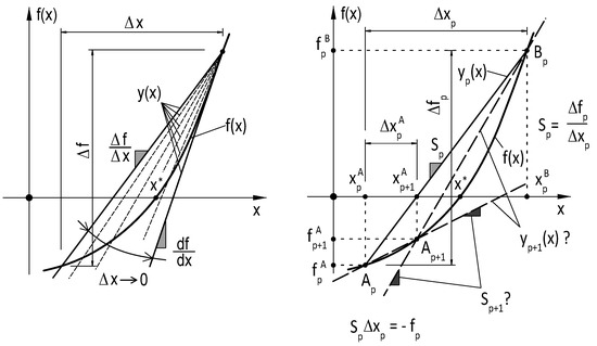
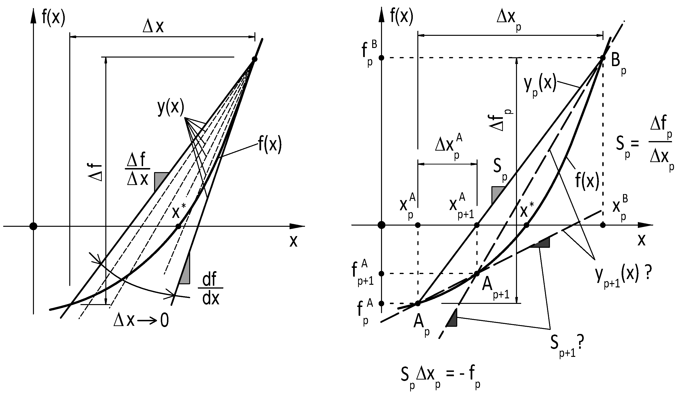
Linearization means that $\mathit{f}\left(\mathit{x}\right)$ is locally replaced by a linear function $\mathit{y}\left(\mathit{x}\right)$ ($\mathit{x}\to \mathit{y}\left(\mathit{x}\right)$, $\mathit{x}\in {\mathbb{R}}^1$, $\mathit{y}:{\mathbb{R}}^1\to {\mathbb{R}}^1$) (secant or tangent line) as shown in Figure 1 (Left) and operations are made on the linear function ${\mathit{y}}_{\mathit{p}}\left(\mathit{x}\right)$ in the ${\mathit{p}}^{\mathit{th}}$ iteration. ${\mathit{y}}_{\mathit{p}}\left(\mathit{x}\right)$ may be defined through two points ${\mathit{A}}_{\mathit{p}}\left({\mathit{x}}_{\mathit{p}}^{\mathit{A}}{\mathit{f}}_{\mathit{p}}^{\mathit{A}}\right)$ and ${\mathit{B}}_{\mathit{p}}\left({\mathit{x}}_{\mathit{p}}^{\mathit{B}}{\mathit{f}}_{\mathit{p}}^{\mathit{B}}\right)$ of the nonlinear function $\mathit{f}\left(\mathit{x}\right)$, where ${\mathit{f}}_{\mathit{p}}^{\mathit{A}}=\mathit{f}\left({\mathit{x}}_{\mathit{p}}^{\mathit{A}}\right)$ and ${\mathit{f}}_{\mathit{p}}^{\mathit{B}}=\mathit{f}\left({\mathit{x}}_{\mathit{p}}^{\mathit{B}}\right)$ are function values, or through one point ${\mathit{A}}_{\mathit{p}}\left({\mathit{x}}_{\mathit{p}}^{\mathit{A}}{\mathit{f}}_{\mathit{p}}^{\mathit{A}}\right)$ and by the “slope”

$${\mathit{S}}_{\mathit{p}}={\displaystyle \frac{▵{\mathit{f}}_{\mathit{p}}}{▵{\mathit{x}}_{\mathit{p}}}}$$

(21)

of the secant line ${\mathit{y}}_{\mathit{p}}\left(\mathit{x}\right)$, where $▵{\mathit{x}}_{\mathit{p}}={\mathit{x}}_{\mathit{p}}^{\mathit{B}}-{\mathit{x}}_{\mathit{p}}^{\mathit{A}}$ and $▵{\mathit{f}}_{\mathit{p}}={\mathit{f}}_{\mathit{p}}^{\mathit{B}}-{\mathit{f}}_{\mathit{p}}^{\mathit{A}}$ are differences, or by the “slope”

$${\mathit{S}}_{\mathit{p}}={\mathit{f}}^{\prime }\left({\mathit{x}}_{\mathit{p}}^{\mathit{A}}\right)={\displaystyle \frac{\mathit{df}}{\mathit{dx}}}$$

(22)

at ${\mathit{x}}_{\mathit{p}}^{\mathit{A}}$ of the tangent line ${\mathit{y}}_{\mathit{p}}\left(\mathit{x}\right)$, where ${\mathit{f}}^{\prime }$ is the derivative function of $\mathit{f}\left(\mathit{x}\right)$. The successive local replacement of the nonlinear function $\mathit{f}\left(\mathit{x}\right)$ by a secant or tangent line ${\mathit{y}}_{\mathit{p}}\left(\mathit{x}\right)$ gives a simple and efficient numerical root-finding procedure. It follows from the condition

$${\mathit{y}}_{\mathit{p}}\left({\mathit{x}}_{p+1}^{\mathit{A}}\right)=0$$

(23)

that the zero

$$x_{p+1}^A={\mathit{x}}_{\mathit{p}}^{\mathit{A}}-{\displaystyle \frac{{\mathit{f}}_{\mathit{p}}^{\mathit{A}}}{{\mathit{S}}_{\mathit{p}}}}$$

(24)

of the linear function ${\mathit{y}}_{\mathit{p}}\left(\mathit{x}\right)$ approximates the zero ${\mathit{x}}^{*}$ of the nonlinear function $\mathit{f}\left(\mathit{x}\right)$, and the new point $A_{p+1}\left({\mathit{x}}_{\mathit{p}+1}^{\mathit{A}}{\mathit{f}}_{\mathit{p}+1}^{\mathit{A}}\right)$ can be determined for the next iteration, as shown in Figure 1 (Right). With the iteration step length

$$▵{\mathit{x}}_{\mathit{p}}^{\mathit{A}}=x_{p+1}^A-{\mathit{x}}_{\mathit{p}}^{\mathit{A}}$$

(25)

from point ${\mathit{A}}_{\mathit{p}}$, Equation (24) can be rewritten as

$${\mathit{S}}_{\mathit{p}}▵{\mathit{x}}_{\mathit{p}}^{\mathit{A}}=-{\mathit{f}}_{\mathit{p}}^{\mathit{A}},$$

(26)

that is called the secant equation, or we may also call it a “linearization” equation, as it also includes Newton’s method as a special case (tangent line). The secant-based procedure has the advantage that it does not need the calculation of function derivatives, it only uses function values and the order of asymptotic convergence is superlinear with convergence rate ${\alpha }^S\cong 1.618\dots$. However, the “slope” of the updated secant line $y_{p+1}\left(x\right)$ can be determined in two ways from the secant (quasi-Newton) conditions as

$$S_{p+1}▵{\mathit{x}}_{\mathit{p}}^{\mathit{A}}={\mathit{f}}_{p+1}^{\mathit{A}}-{\mathit{f}}_{\mathit{p}}^{\mathit{A}}$$

(27)

or

$$S_{p+1}▵{\mathit{x}}_{\mathit{p}}^{\mathit{B}}={\mathit{f}}_{p+1}^{\mathit{A}}-{\mathit{f}}_{\mathit{p}}^{\mathit{B}},$$

(28)

where

$$▵{\mathit{x}}_{\mathit{p}}^{\mathit{B}}=x_{p+1}^A-{\mathit{x}}_{\mathit{p}}^{\mathit{B}}$$

(29)

is the iteration step length from point ${\mathit{B}}_{\mathit{p}}$. The decision is far from obvious, as shown in Figure 1 (Right). The tangent-line-based iteration (Newton’s method) has an advantage that the “slope”

$$S_{p+1}=f^{\prime }\left({\mathit{x}}_{p+1}^{\mathit{A}}\right)$$

(30)

of the updated tangent line is always well defined. The iteration then continues with the updated secant or tangent line $y_{p+1}\left(x\right)$.

Figure 1. Left: linearization of a nonlinear function; Right: classic secant method.

3.2. Multi-Variable Case

The scalar linearization procedure can be extended to multi-dimensions. The zero ${\mathit{x}}^{*}$ of a nonlinear vector-valued function

$$\mathit{f}\left(\mathit{x}\right)=\left[\begin{array}{c}{\mathit{f}}_{\mathit{1}}\left(\mathit{x}\right)\\ ⋮\\ {\mathit{f}}_{\mathit{m}}\left(\mathit{x}\right)\end{array}\right]$$

(31)

of $\mathit{n}$ variables

$$\mathit{x}=\left[\begin{array}{c}{x}_1\\ ⋮\\ x_n\end{array}\right]$$

(32)

($\mathit{x}\to \mathit{f}\left(\mathit{x}\right)$, $\mathit{x}\in {\mathbb{R}}^{\mathit{n}},\mathit{f}:{\mathbb{R}}^{\mathit{n}}\to {\mathbb{R}}^{\mathit{m}},\mathit{n}\le \mathit{m}$) has to be determined, where

$$\mathit{f}\left({\mathit{x}}^{*}\right)=0.$$

(33)

Then, $\mathit{f}\left(\mathit{x}\right)$ is locally replaced by an $\mathit{n}$-dimensional hyperplane

$$\mathit{y}\left(\mathit{x}\right)(\mathit{x}\to \mathit{y}\left(\mathit{x}\right),\mathit{x}\in {\mathbb{R}}^{\mathit{n}},\mathit{y}:{\mathbb{R}}^{\mathit{n}}\to {\mathbb{R}}^{\mathit{m}}$$

(34)

$\left(\mathit{n}\le \mathit{m}\right)$ and operations are made on the hyperplane ${\mathit{y}}_{\mathit{p}}\left(\mathit{x}\right)$ in the ${\mathit{p}}^{\mathit{th}}$ iteration. ${\mathit{y}}_{\mathit{p}}\left(\mathit{x}\right)$ may be defined through $n+1$ points ${\mathit{A}}_{\mathit{p}}\left({\mathit{x}}_{\mathit{p}}^{\mathit{A}}{\mathit{f}}_{\mathit{p}}^{\mathit{A}}\right)$ and ${\mathit{B}}_{\mathit{k},\mathit{p}}\left({\mathit{x}}_{\mathit{k},\mathit{p}}^{\mathit{B}}{\mathit{f}}_{\mathit{k},\mathit{p}}^{\mathit{B}}\right)$ ($k=1,\dots ,n$) of the nonlinear function $\mathit{f}\left(\mathbf{x}\right)$, where ${\mathit{f}}_{\mathit{p}}^{\mathit{A}}=\mathit{f}\left({\mathit{x}}_{\mathit{p}}^{\mathit{A}}\right)$ and ${\mathit{f}}_{\mathit{k},\mathit{p}}^{\mathit{B}}=\mathit{f}\left({\mathit{x}}_{\mathit{k},\mathit{p}}^{\mathit{B}}\right)$ ($k=1,\dots ,n$) are function values, or by one point ${\mathit{A}}_{\mathit{p}}\left({\mathit{x}}_{\mathit{p}}^{\mathit{A}}{\mathit{f}}_{\mathit{p}}^{\mathit{A}}\right)$ and by the “slope” (divided differences)

$${\mathit{S}}_{\mathit{p}}=▵{\mathit{F}}_{\mathit{p}}▵{\mathit{X}}_{\mathit{p}}^{-1}$$

(35)

$\left(\mathit{i}=1,\dots ,\mathit{n}\right)$, $\left(j=1,\dots ,m\right)$, $\left(\mathit{k}=1,\dots ,\mathit{n}\right)$ of the $\mathit{n}$-dimensional secant hyperplane ${\mathit{y}}_{\mathit{p}}\left(\mathit{x}\right)$, where $▵{\mathit{x}}_{\mathit{k},\mathit{p}}={\mathit{x}}_{\mathit{k},\mathit{p}}^{\mathit{B}}-{\mathit{x}}_{\mathit{p}}^{\mathit{A}}$ and $▵{\mathit{f}}_{\mathit{k},\mathit{p}}={\mathit{f}}_{\mathit{k},\mathit{p}}^{\mathit{B}}-{\mathit{f}}_{\mathit{p}}^{\mathit{A}}$ are difference vectors with $\mathit{n}$ and $\mathit{m}$ components, respectively, and

$$▵{\mathit{F}}_p=\left[▵{\mathit{f}}_{k,p}\right]=\left[{\mathit{f}}_{k,p}^B-{\mathit{f}}_p^A\right]=\left[\begin{array}{ccc}▵f_{1,1,p}& \cdots & ▵f_{n,1,p}\\ ⋮& \ddots & ⋮\\ ▵f_{1,m,p}& \cdots & ▵f_{n,m,p}\end{array}\right],$$

(36)

$$▵{\mathit{X}}_p=\left[▵{\mathit{x}}_{k,p}\right]=\left[{\mathit{x}}_{k,p}^B-{\mathit{x}}_p^A\right]=\left[\begin{array}{ccc}▵x_{1,1,p}& \cdots & ▵x_{n,1,p}\\ ⋮& ⋮& ⋮\\ ▵x_{1,n,p}& \cdots & ▵x_{n,n,p}\end{array}\right].$$

(37)

The $\mathit{n}$-dimensional tangent hyperplane ${\mathit{y}}_{\mathit{p}}\left(\mathit{x}\right)$ through point ${\mathit{A}}_{\mathit{p}}\left({\mathit{x}}_{\mathit{p}}^{\mathit{A}}{\mathit{f}}_{\mathit{p}}^{\mathit{A}}\right)$ may be defined by the “slope”

$${\mathit{S}}_p=\left[{\displaystyle \frac{\partial f_{k,j,p}}{\partial x_{k,i,p}}}\right]=\left[\begin{array}{ccc}{\displaystyle \frac{\partial f_{1,1,\mathrm{p}}}{\partial x_{1,\mathrm{p}}}}& \dots & {\displaystyle \frac{\partial f_{n,1,\mathrm{p}}}{\partial x_{n,p}}}\\ ⋮& ⋮& ⋮\\ {\displaystyle \frac{\partial f_{1,\mathrm{m},\mathrm{p}}}{\partial x_{1,\mathrm{p}}}}& \cdots & {\displaystyle \frac{\partial f_{n,\mathrm{m},\mathrm{p}}}{\partial x_{n,p}}}\end{array}\right],$$

(38)

that corresponds to the Jacobian matrix ${\mathit{J}}_{\mathit{p}}$ of the nonlinear vector-valued function $\mathit{f}\left(\mathit{x}\right)$, and accordingly, Definition (35) corresponds to the approximation of the Jacobian matrix. It follows from the condition

$${\mathit{y}}_{\mathit{p}}\left({\mathit{x}}_{p+1}^{\mathit{A}}\right)=\mathit{0}$$

(39)

that the zero

$${\mathit{x}}_{p+1}^A={\mathit{x}}_{\mathit{p}}^{\mathit{A}}-{\mathit{S}}_{\mathit{p}}^{+}{\mathit{f}}_{\mathit{p}}^{\mathit{A}}$$

(40)

of the $\mathit{n}$-dimensional hyperplane $\mathit{y}\left(\mathit{x}\right)$ approximates the zero ${\mathit{x}}^{*}$ of the nonlinear vector-valued function $\mathit{f}\left(\mathit{x}\right)$, where ${\left[.\right]}^{+}$ stands for the pseudoinverse. Then, the ${\mathit{i}}^{\mathit{th}}$ element of the new approximate ${\mathit{x}}_{\mathit{p}+1}^{\mathit{A}}$ in the ${\mathit{p}}^{\mathit{th}}$ iteration will be

$${\mathit{x}}_{i,p+1}^{\mathit{A}}={\mathit{x}}_{\mathit{i},\mathit{p}}^{\mathit{A}}-\sum _{\mathit{j}=1}^{\mathit{m}}\left({\mathit{S}}_{\mathit{i},\mathit{j},\mathit{p}}^{+}{\mathit{f}}_{\mathit{j},\mathit{p}}^{\mathit{A}}\right)$$

(41)

$\left(i=1,\dots ,n\right),\left(j=1,\dots ,m\right)$. With the iteration stepsize

$$▵{\mathit{x}}_{\mathit{p}}^{\mathit{A}}={\mathit{x}}_{p+1}^A-{\mathit{x}}_{\mathit{p}}^{\mathit{A}}=-{\mathit{S}}_{\mathit{p}}^{+}{\mathit{f}}_{\mathit{p}}^{\mathit{A}}=-\left[{\left(\sum _{\mathit{j}=1}^{\mathit{m}}\left({\mathit{S}}_{\mathit{i},\mathit{j},\mathit{p}}^{+}{\mathit{f}}_{\mathit{j},\mathit{p}}^{\mathit{A}}\right)\right)}_i\right],$$

(42)

Equation (40) can be rewritten as

$${\mathit{S}}_{\mathit{p}}▵{\mathit{x}}_{\mathit{p}}^{\mathit{A}}=-{\mathit{f}}_{\mathit{p}}^{\mathit{A}},$$

(43)

which is called “secant equation” or “linearization equation” in the multi-variable case. With the new approximate ${\mathit{x}}_{p+1}^{\mathit{A}}$ and with the corresponding function value ${\mathit{f}}_{p+1}^{\mathit{A}}$, an updated Jacobian or Jacobian approximate ${\mathit{S}}_{p+1}$ has to be determined. Table 1 summarizes the basic equations of the above-detailed linearization methods.

Table 1. Linearization method’s basic equations (single- and multi-variable cases).

	Single-Variable $\left(\mathit{m}=\mathit{n}=1\right)$	Multi-Variable $\left(\mathit{m}\ge \mathit{n}>1\right)$	Equations
1	$▵x_{\mathit{p}}={\mathit{x}}_{\mathit{p}}^{\mathit{B}}-{\mathit{x}}_{\mathit{p}}^{\mathit{A}}$	$▵{\mathit{X}}_{\mathit{p}}=\left[\begin{array}{ccc}▵{\mathit{x}}_{\mathit{1},\mathit{1},\mathit{p}}& \cdots & ▵{\mathit{x}}_{\mathit{n},\mathit{1},\mathit{p}}\\ ⋮& ⋮& ⋮\\ ▵{\mathit{x}}_{\mathit{1},\mathit{n},\mathit{p}}& \cdots & ▵{\mathit{x}}_{\mathit{n},\mathit{n},\mathit{p}}\end{array}\right]$	(37)
2	$▵{\mathit{f}}_{\mathit{p}}={\mathit{f}}_{\mathit{p}}^{\mathit{B}}-{\mathit{f}}_{\mathit{p}}^{\mathit{A}}$	$▵{\mathit{F}}_{\mathit{p}}=\left[\begin{array}{ccc}▵f_{p,1,1}& \cdots & ▵f_{p,n,1}\\ ⋮& \ddots & ⋮\\ ▵f_{p,1,m}& \cdots & ▵{\mathit{f}}_{\mathit{p},\mathit{n},\mathit{m}}\end{array}\right]$	(36)
3	${\mathit{S}}_{\mathit{p}}={\displaystyle \frac{▵{\mathit{f}}_{\mathit{p}}}{▵{\mathit{x}}_{\mathit{p}}}}$	${\mathit{S}}_{\mathit{p}}=▵{\mathit{F}}_{\mathit{p}}▵{\mathit{X}}_{\mathit{p}}^{-1}$	(21) and (35)
4	$x_{p+1}^A=x_p^A-{\displaystyle \frac{{\mathit{f}}_{\mathit{p}}^{\mathit{A}}}{{\mathit{S}}_{\mathit{p}}}}$	${\mathit{x}}_{\mathit{p}+1}^{\mathit{A}}={\mathit{x}}_{\mathit{p}}^{\mathit{A}}-{\mathit{S}}_{\mathit{p}}^{+}{\mathit{f}}_{\mathit{p}}^{\mathit{A}}$	(24) and (40)
5	$S_{p+1}▵{\mathit{x}}_{\mathit{p}}^{\mathit{A}}=f_{p+1}^{\mathit{A}}-{\mathit{f}}_{\mathit{p}}^{\mathit{A}}$	${\mathit{S}}_{p+1}▵{\mathit{x}}_{\mathit{p}}^{\mathit{A}}={\mathit{f}}_{p+1}^{\mathit{A}}-{\mathit{f}}_{\mathit{p}}^{\mathit{A}}$	(27) and (45)

If all partial derivatives of the function $\mathit{f}\left(\mathit{x}\right)$ are known, then the Jacobian update can easily be calculated. Newton’s method is one of the most widely used algorithms, with very attractive theoretical and practical properties and with some limitations. The computational costs of Newton’s method are high, since the Jacobian ${\mathit{J}}_{\mathit{p}}$ and the solution to the linear system (43) must be computed at each iteration. It is well known that the local convergence of Newton’s method is $\mathit{q}$-quadratic if the initial trial approximate ${\mathit{x}}_0$ is close enough to the solution ${\mathit{x}}^{*}$, if $\mathit{J}\left({\mathit{x}}^{*}\right)$ is nonsingular, and if $\mathit{J}\left(\mathit{x}\right)$ satisfies the Lipschitz condition

$$∥\mathit{J}\left(\mathbf{x}\right)-\mathit{J}\left({\mathit{x}}^{*}\right)∥\le \mathit{L}∥\mathit{x}-{\mathit{x}}^{*}∥$$

(44)

for all $\mathit{x}$ close enough to ${\mathit{x}}^{*}$.

However, in many cases, the function $\mathit{f}\left(\mathit{x}\right)$ is not an analytical function, the partial derivatives are not known or difficult to evaluate, and Newton’s method cannot be applied. Quasi-Newton methods are widely used for solving systems of nonlinear equations when the Jacobian is not known or difficult to determine. The Jacobian is approximated by divided differences (35), and the system of nonlinear Equations (5) is solved by repeatedly solving systems of linear Equations (43) providing the new approximates ${\mathit{x}}_{\mathit{p}+1}^{\mathit{A}}$.

The Jacobian approximate (35) should be updated according to the fundamental equation of the quasi-Newton methods (“quasi-Newton condition” or “secant condition”)

$${\mathit{S}}_{p+1}▵{\mathit{x}}_{\mathit{p}}^{\mathit{A}}={\mathit{f}}_{p+1}^{\mathit{A}}-{\mathit{f}}_{\mathit{p}}^{\mathit{A}}$$

(45)

for all $\mathit{p}=0,1,2,\dots$. However, the condition (45) does not uniquely specify the update ${\mathit{S}}_{\mathit{p}+1}$, so the iterative procedure is not well defined and further constraints are needed. Different methods offer their own specific solution, but new quasi-Newton approximate ${\mathit{x}}_{\mathit{p}+1}$ will never allow full-rank update of the Jacobian approximate ${\mathit{S}}_{\mathit{p}+1}$ (Equation (45) is an underdetermined system of $\mathit{m}$ linear equations with $\mathit{mn}$ unknowns). A large family of methods is available with different additional conditions or assumptions. Martinez [31] has been made a thorough survey on the family of practical quasi-Newton methods.

The partial derivatives of the Jacobian matrix may be replaced by suitable difference quotients (discretized Newton iteration; see [1,2])

$$\left[{\displaystyle \frac{▵\mathit{f}}{▵\mathit{x}}}\right]=\left[{\displaystyle \frac{{\mathit{f}}_j\left(\mathit{x}+▵{\mathit{x}}_k{\mathit{d}}^k\right)-{\mathit{f}}_j\left(\mathit{x}\right)}{▵{\mathit{x}}_k}}\right]=\left[{\displaystyle \frac{▵{\mathit{f}}_j\left(\mathit{x}\right)}{▵{\mathit{x}}_k}}\right]$$

(46)

$\left(k=1,\dots ,n\right)$, $\left(j=1,\dots ,m\right)$ with $\mathit{n}$ additional function value evaluations, where ${\mathit{d}}^{\mathit{k}}$ is the ${\mathit{k}}^{\mathit{th}}$ Cartesian unit vector. However, it is difficult to choose the stepsize $▵\mathit{x}$. If any $▵{\mathit{x}}_{\mathit{k}}$ is too large, then Expression (46) can be a bad approximation to the Jacobian so the iteration converges much more slowly, if it converges at all. On the other hand, if any $▵{\mathit{x}}_{\mathit{k}}$ is too small, then $▵{\mathit{f}}_{\mathit{j}}\left(\mathit{x}\right)\simeq 0$, and cancellations can occur, which reduces the accuracy of the difference quotients (46) (see [32]). Another modification is the inexact-Newton approach, when the nonlinear equation is solved by an iterative linear solver (see [33,34,35]). Wolfe [10] and Popper [9] suggested the column update of matrix (36).

One of the most widely used formulas is that of Broyden [36], which makes a rank-one update for the Jacobian approximate as

$${\mathit{S}}_{p+1}={\mathit{S}}_p+{\mathit{Q}}_p={\mathit{S}}_p+{\displaystyle \frac{▵{\mathit{f}}_{\mathit{p}}^{\mathit{A}}-{\mathit{S}}_p▵{\mathit{x}}_{\mathit{p}}^{\mathit{A}}}{{∥▵{\mathit{x}}_{\mathit{p}}^{\mathit{A}}∥}^2}}{\left[▵{\mathit{x}}_{\mathit{p}}^{\mathit{A}}\right]}^T,$$

(47)

where ${\mathit{Q}}_{\mathit{p}}$ is a rank-one matrix, and by using the Sherman–Morrison formula, the inverse Jacobian approximate update is given as

$${\mathit{S}}_{p+1}^{+}={\mathit{S}}_p^{+}+{\displaystyle \frac{▵{\mathit{x}}_{\mathit{p}}^{\mathit{A}}-{\mathit{S}}_p^{+}▵{\mathit{f}}_{\mathit{p}}^{\mathit{A}}}{{\left[▵{\mathit{x}}_{\mathit{p}}^{\mathit{A}}\right]}^T{\mathit{S}}_p^{+}▵{\mathit{f}}_{\mathit{p}}^{\mathit{A}}}}{\left[▵{\mathit{x}}_{\mathit{p}}^{\mathit{A}}\right]}^T{\mathit{S}}_p^{+}.$$

(48)

Broyden’s secant condition (45) can be rewritten as

$${\mathit{S}}_p▵{\mathit{x}}_{\mathit{p}}^{\mathit{A}}+{\mathit{Q}}_p▵{\mathit{x}}_{\mathit{p}}^{\mathit{A}}={\mathit{f}}_{p+1}^{\mathit{A}}-{\mathit{f}}_{\mathit{p}}^{\mathit{A}},$$

(49)

and with the secant Equation (43), we have

$${\mathit{Q}}_p▵{\mathit{x}}_{\mathit{p}}^{\mathit{A}}={\mathit{f}}_{p+1}^{\mathit{A}}.$$

(50)

As ${\mathit{Q}}_{\mathit{p}}$ is a rank-one matrix, then this equation has an infinitely large number of solutions (the left nullspace of matrix ${\mathit{Q}}_{\mathit{p}}$ is an $n-1$ dimensional vector space [37]), and the Ortega–Rheinboldt [2] condition will not be satisfied (the column vectors of matrix ${\mathit{S}}_{\mathit{p}}$ should be linearly independent and have to be “in general position” through the whole iteration process) and it may result an ill-conditioned Broyden update ${\mathit{S}}_{p+1}$.

4. T-Secant Method

A numerical procedure has been developed for solving an overdetermined system of nonlinear Equations (5). It can be considered both as a discretized Newton’s method or as a quasi-Newton method with full-rank update of the Jacobian approximates. The suggested full-rank update procedure (“T-Secant” method [5]) provides an unconventional and simple strategy to improve the performance of quasi-Newton iterations. It is based on the classic secant linearization, which was completed with a new independent approximate ${\mathit{x}}_{p+1}^B$. The secant equation was modified by a suitably chosen nonuniform scaling transformation and a new independent approximate ${\mathit{x}}_{p+1}^B$ was determined from the modified secant equation. The solution to the secant equation presented in [5] was based on the Wolfe–Popper procedure [9,10] so that the secant equation was splitted into two equations by introducing an auxiliary variable. The simplified algorithm, presented in this paper, directly solves the secant equation by using the pseudoinverse of the transformed Jacobian approximate.

4.1. Single-Variable Case

The suggested procedure uses the information on the improvement of the classic secant procedure and gives a new approximate $x_{p+1}^B$ in the vicinity of the classic secant approximate $x_{p+1}^A$ as follows. Given two initial approximates ${\mathit{x}}_{\mathit{p}}^{\mathit{A}}$ and ${\mathit{x}}_{\mathit{p}}^{\mathit{B}}$ with function values ${\mathit{f}}_{\mathit{p}}^{\mathit{A}}$ and ${\mathit{f}}_{\mathit{p}}^{\mathit{B}}$, the new approximate $x_{p+1}^A$ with function value $f_{p+1}^A$ is known from the solution of the classic secant Equation (26). An independent new approximate

$$x_{p+1}^B=x_{p+1}^A+▵{\mathit{x}}_{p+1}$$

(51)

is planned to be determined in the vicinity of the classic secant approximate $x_{p+1}^A$. Let the ratio

$${\mathit{t}}_{\mathit{p}}^f={\displaystyle \frac{{\mathit{f}}_{\mathit{p}+1}^{\mathit{A}}}{{\mathit{f}}_{\mathit{p}}^{\mathit{A}}}}$$

(52)

$\left({\mathit{f}}_{\mathit{p}}^{\mathit{A}}\ne \mathit{0}\right)$ of the function value improvement and the ratio

$${\mathit{t}}_{\mathit{p}}^{\mathit{x}}={\displaystyle \frac{{\mathit{x}}_{\mathit{p}+1}^{\mathit{B}}-{\mathit{x}}_{\mathit{p}+1}^{\mathit{A}}}{{\mathit{x}}_{\mathit{p}+1}^{\mathit{A}}-{\mathit{x}}_{\mathit{p}}^{\mathit{A}}}}={\displaystyle \frac{▵{\mathit{x}}_{p+1}}{▵{\mathit{x}}_{\mathit{p}}^{\mathit{A}}}}$$

(53)

$\left(▵{\mathit{x}}_{\mathit{p}}^{\mathit{A}}\ne \mathit{0}\right)$ of the desired iteration stepsize change be defined. The single-variable secant Equation (26) is then modified as

$${\mathit{S}}_{\mathit{Tp}}▵{\mathit{x}}_{\mathit{p}}^{\mathit{A}}=-{\mathit{f}}_{\mathit{p}}^{\mathit{A}},$$

(54)

where

$${\mathit{S}}_{\mathit{Tp}}={\displaystyle \frac{{\mathit{t}}_{\mathit{p}}^{\mathit{f}}}{{\mathit{t}}_{\mathit{p}}^{\mathit{x}}}}{\mathit{S}}_{\mathit{p}}.$$

(55)

Then, the new approximate $x_{p+1}^B$ can be expressed from Equation (54) as

$${\mathit{t}}_{\mathit{p}}^{\mathit{f}}{\displaystyle \frac{{\mathit{x}}_{\mathit{p}+1}^{\mathit{A}}-{\mathit{x}}_{\mathit{p}}^{\mathit{A}}}{{\mathit{x}}_{\mathit{p}+1}^{\mathit{B}}-{\mathit{x}}_{\mathit{p}+1}^{\mathit{A}}}}{\mathit{S}}_{\mathit{p}}▵{\mathit{x}}_{\mathit{p}}^{\mathit{A}}=-{\mathit{f}}_{\mathit{p}}^{\mathit{A}}.$$

(56)

After rearrangement, we obtain

$${\mathit{x}}_{\mathit{p}+1}^{\mathit{A}}-{\mathit{x}}_{\mathit{p}+1}^{\mathit{B}}={\displaystyle \frac{{\mathit{t}}_{\mathit{p}}^{\mathit{f}}}{{\mathit{f}}_{\mathit{p}}^{\mathit{A}}}}{\mathit{S}}_{\mathit{p}}{\left(▵{\mathit{x}}_{\mathit{p}}^{\mathit{A}}\right)}^{\mathit{2}}$$

(57)

and with the secant Equation (26), it turns to

$$x_{p+1}^B=x_{p+1}^A-{\displaystyle \frac{t_p^{\mathit{f}}}{{\mathit{f}}_{\mathit{p}}^{\mathit{A}}}}{S}_p{\left(▵{\mathit{x}}_{\mathit{p}}^{\mathit{A}}\right)}^2=x_{p+1}^A+t_p^{\mathit{f}}▵{\mathit{x}}_{\mathit{p}}^{\mathit{A}}$$

(58)

and the desired new iteration stepsize

$$▵{\mathit{x}}_{p+1}=t_p^{\mathit{f}}▵{\mathit{x}}_{\mathit{p}}^{\mathit{A}}$$

(59)

can be given. The suggested procedure can also be applied to Newton’s method (T-Newton method). Then, the “slope” ${\mathit{S}}_{\mathit{p}}$ corresponds to the derivative ${\mathit{f}}^{\prime }$ of function $\mathit{f}\left(\mathit{x}\right)$.

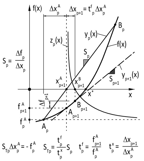
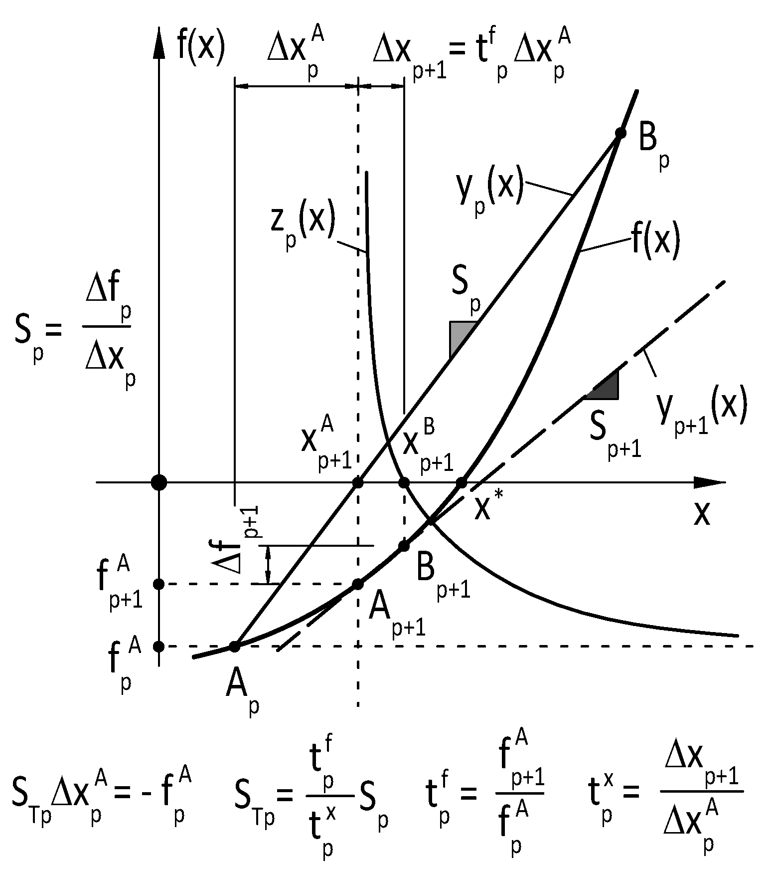
The geometrical representation of the suggested method can be derived as follows ([5]). Let the new approximate $x_{p+1}^B$ be the zero of a function ${\mathit{z}}_{\mathit{p}}\left(\mathit{x}\right)$ :

$$z_p\left(x_{p+1}^{\mathit{B}}\right)=0.$$

(60)

Then, replacing $x_{p+1}^B$ with $\mathit{x}$ in Equation (58) gives the function

$${\mathit{z}}_{\mathit{p}}\left(\mathit{x}\right)={\displaystyle \frac{{\mathit{t}}_{\mathit{p}}^{\mathit{f}}{\mathit{S}}_{\mathit{p}}{\left(▵{\mathit{x}}_{\mathit{p}}^{\mathit{A}}\right)}^{\mathit{2}}}{\mathit{x}-{\mathit{x}}_{\mathit{p}+1}^{\mathit{A}}}}+{\mathit{f}}_{\mathit{p}}^{\mathit{A}}=0$$

(61)

with zero at

$$x=x_{p+1}^B.$$

(62)

Equation (61) is a hyperbolic function with vertical and horizontal asymptotes ${\mathit{x}}_{\mathit{p}+1}^{\mathit{A}}$ and ${\mathit{f}}_{\mathit{p}}^{\mathit{A}}$, and its root ${\mathit{x}}_{p+1}^{\mathit{B}}$ will be in the vicinity of ${\mathit{x}}_{p+1}^{\mathit{A}}$ in an “appropriate distance” that is regulated by the function value ${\mathit{f}}_{p+1}^{\mathit{A}}$ (see Figure 2). This virtue of the suggested procedure ensures an automatic mechanism for having the actual approximates ${\mathit{x}}_{\mathit{p}}^{\mathit{A}}$ and ${\mathit{x}}_{\mathit{p}}^{\mathit{B}}$ in general positions through the whole iteration process providing stable and efficient numerical performance. The suggested method’s performance is demonstrated with the results of numerical tests on test functions in Section 6.

Figure 2. Suggested full-rank update method (T-secant).

4.2. Multi-Variable Case

Let two independent approximates ${\mathit{x}}_{\mathit{p}}^{\mathit{A}}=\left[{\mathit{x}}_{\mathit{k},\mathit{p}}^{\mathit{A}}\right]$ and ${\mathit{x}}_{\mathit{p}}^{\mathit{B}}=\left[{\mathit{x}}_{\mathit{k},\mathit{p}}^{\mathit{B}}\right]$ to the zero ${\mathit{x}}^{*}$ of the nonlinear vector-valued function $\mathit{f}\left(\mathit{x}\right)$ be given in the ${\mathit{p}}^{\mathit{th}}$ iteration $\left(k=1,\dots ,n\right)$. Let the series of $\mathit{n}$ approximates ${\mathit{x}}_{\mathit{k},\mathit{p}}^{\mathit{B}}$ be constructed by individually increment the elements ${\mathit{x}}_{\mathit{k},\mathit{p}}^{\mathit{A}}$ of the approximate ${\mathbf{x}}_{\mathit{p}}^{\mathit{A}}$ by an increment

$$▵{\mathit{x}}_{\mathit{k},\mathit{p}}={\mathit{x}}_{\mathit{k},\mathit{p}}^{\mathit{B}}-{\mathit{x}}_{\mathit{k},\mathit{p}}^{\mathit{A}}$$

(63)

as

$${\mathit{x}}_{\mathit{k},\mathit{p}}^{\mathit{B}}={\mathit{x}}_{\mathit{p}}^{\mathit{A}}+▵{\mathit{x}}_{\mathit{k},\mathit{p}}{\mathit{d}}^{\mathit{k}}$$

(64)

where ${\mathit{d}}^{\mathit{k}}$ is the ${\mathit{k}}^{\mathit{th}}$ Cartesian unit vector. It follows from this special construction of the approximates ${\mathit{x}}_{\mathit{k},\mathit{p}}^{\mathit{B}}$ that ${\mathit{x}}_{\mathit{k},\mathit{i},\mathit{p}}^{\mathit{B}}-{\mathit{x}}_{\mathit{k},\mathit{p}}^{\mathit{A}}=0$ for $\mathit{i}\ne \mathit{k}$ and ${\mathit{x}}_{\mathit{k},\mathit{i},\mathit{p}}^{\mathit{B}}-{\mathit{x}}_{\mathit{k},\mathit{p}}^{\mathit{A}}=▵{\mathit{x}}_{\mathit{k},\mathit{p}}$ for $\mathit{i}=\mathit{k}$, and matrix (37) will be a diagonal matrix:

$$▵{\mathit{X}}_{\mathit{p}}=\left[▵{\mathit{x}}_{\mathit{k},\mathit{p}}\right]=\left[{\mathit{x}}_{\mathit{k},\mathit{p}}^{\mathit{B}}-{\mathit{x}}_{\mathit{p}}^{\mathit{A}}\right]=\left[\begin{array}{ccc}▵x_{1,\mathit{p}}& \cdots & 0\\ ⋮& \ddots & ⋮\\ 0& \cdots & ▵x_{\mathit{n},\mathit{p}}\end{array}\right]=\mathit{diag}\left(▵x_{\mathit{k},\mathit{p}}\right).$$

(65)

Let the ratios

$${\mathit{T}}_{\mathit{p}}^{\mathit{F}}=\mathit{diag}\left({\mathit{t}}_{\mathit{j},\mathit{p}}^{\mathit{F}}\right)=\mathit{diag}\left({\displaystyle \frac{f_{j,p+1}^{\mathit{A}}}{{\mathit{f}}_{\mathit{j},\mathit{p}}^{\mathit{A}}}}\right)$$

(66)

$\left({\mathit{f}}_{j,p}^A\ne 0\right)$ of the function value improvements $\left(j=1,\dots ,m\right)$ and the ratios

$${\mathit{T}}_{\mathit{p}}^X=\mathit{diag}\left({\mathit{t}}_{\mathit{i},\mathit{p}}^{\mathit{X}}\right)=\mathit{diag}\left({\displaystyle \frac{{\mathit{x}}_{\mathit{i},\mathit{p}+1}^{\mathit{B}}-{\mathit{x}}_{\mathit{i},\mathit{p}+1}^{\mathit{A}}}{{\mathit{x}}_{\mathit{i},\mathit{p}+1}^{\mathit{A}}-{\mathit{x}}_{\mathit{i},\mathit{p}}^{\mathit{A}}}}\right)=\mathit{diag}\left({\displaystyle \frac{▵{\mathit{x}}_{\mathit{i},\mathit{p}+1}}{▵{\mathit{x}}_{\mathit{i},\mathit{p}}^{\mathit{A}}}}\right)$$

(67)

$\left(▵{\mathit{x}}_{\mathit{i},\mathit{p}}^{\mathit{A}}\ne 0\right)$ of the desired iteration stepsize changes $\left(i=1,\dots ,n\right)$ be defined similarly as in the single-variable case. Let the secant Equation (43) be modified as

$${\mathit{S}}_{\mathit{Tp}}▵{\mathit{x}}_{\mathit{p}}^{\mathit{A}}=-{\mathit{f}}_{\mathit{p}}^{\mathit{A}},$$

(68)

where

$${\mathit{S}}_{\mathit{Tp}}={\mathit{T}}_{\mathit{p}}^{\mathit{F}}{\mathit{S}}_{\mathit{p}}{\left({\mathit{T}}_{\mathit{p}}^{\mathit{X}}\right)}^{-1}=\mathit{diag}\left({\mathit{t}}_{\mathit{j},\mathit{p}}^{\mathit{F}}\right)\left[{\displaystyle \frac{▵{\mathit{f}}_{\mathit{k},\mathit{j},\mathit{p}}}{▵{\mathit{x}}_{\mathit{i},\mathit{p}}}}\right]\mathit{diag}\left({\displaystyle \frac{1}{{\mathit{t}}_{\mathit{i},\mathit{p}}^{\mathit{X}}}}\right)=\left[{\displaystyle \frac{{\mathit{t}}_{\mathit{j},\mathit{p}}^{\mathit{F}}}{{\mathit{t}}_{\mathit{i},\mathit{p}}^{\mathit{X}}}}{\displaystyle \frac{▵{\mathit{f}}_{\mathit{k},\mathit{j},\mathit{p}}}{▵{\mathit{x}}_{\mathit{i},\mathit{p}}}}\right],$$

(69)

$\left(\mathit{i}=1,\dots ,\mathit{n}\right)$, $\left(\mathit{j}=1,\dots ,\mathit{m}\right)$, $\left(\mathit{k}=1,\dots ,\mathit{n}\right)$ or in explicit form:

$${\mathit{S}}_{\mathit{Tp}}=\left[\begin{array}{ccc}{\displaystyle \frac{{\mathit{f}}_{\mathit{1},\mathit{p}+1}^{\mathit{A}}}{{\mathit{f}}_{1,\mathit{p}}^{\mathit{A}}}}& 0& 0\\ 0& \ddots & 0\\ 0& 0& {\displaystyle \frac{{\mathit{f}}_{\mathit{m},\mathit{p}+1}^{\mathit{A}}}{{\mathit{f}}_{\mathit{m},\mathit{p}}^{\mathit{A}}}}\end{array}\right]\left[\begin{array}{ccc}{\displaystyle \frac{▵{\mathit{f}}_{1,1,\mathit{p}}}{▵{\mathit{x}}_{1,\mathit{p}}}}& \dots & {\displaystyle \frac{▵{\mathit{f}}_{1,\mathit{n},\mathit{p}}}{▵{\mathit{x}}_{\mathit{n},\mathit{p}}}}\\ ⋮& ⋮& ⋮\\ {\displaystyle \frac{▵{\mathit{f}}_{1,\mathit{m},\mathit{p}}}{▵{\mathit{x}}_{1,\mathit{p}}}}& \cdots & {\displaystyle \frac{▵{\mathit{f}}_{\mathit{n},\mathit{m},\mathit{p}}}{▵{\mathit{x}}_{\mathit{n},\mathit{p}}}}\end{array}\right]\left[\begin{array}{ccc}{\displaystyle \frac{▵x_{1,p}^{\mathit{A}}}{▵x_{1,p+1}}}& 0& 0\\ 0& \ddots & 0\\ 0& 0& {\displaystyle \frac{▵{\mathit{x}}_{\mathit{n},\mathit{p}}^{\mathit{A}}}{▵x_{n,p+1}}}\end{array}\right],$$

(70)

and

$${\mathit{S}}_{\mathit{Tp}}^{+}={\mathit{T}}_{\mathit{p}}^{\mathit{X}}{\mathit{S}}_{\mathit{p}}^{+}{\left({\mathit{T}}_{\mathit{p}}^{\mathit{F}}\right)}^{-1}$$

(71)

is the pseudoinverse of ${\mathit{S}}_{\mathit{p}}$. Then, Equation (68) can be rewritten as

$$▵{\mathit{x}}_{\mathit{p}}^{\mathit{A}}=-{\mathit{S}}_{\mathit{Tp}}^{+}{\mathit{f}}_{\mathit{p}}^{\mathit{A}}.$$

(72)

Then, the ${\mathit{i}}^{\mathit{th}}$ element ${\mathit{x}}_{\mathit{i},\mathit{p}+1}^{\mathit{B}}$ of the new approximate ${\mathit{x}}_{\mathit{p}+1}^{\mathit{B}}$ in the ${\mathit{p}}^{\mathit{th}}$ iteration will be

$${\mathit{x}}_{\mathit{i},\mathit{p}+1}^{\mathit{B}}={\mathit{x}}_{\mathit{i},\mathit{p}+1}^{\mathit{A}}+▵{\mathit{x}}_{\mathit{i},\mathit{p}+1}={\mathit{x}}_{\mathit{i},\mathit{p}+1}^{\mathit{A}}-{\displaystyle \frac{{\left(▵{\mathit{x}}_{\mathit{i},\mathit{p}}^{\mathit{A}}\right)}^2}{{\displaystyle \sum _{\mathit{j}=1}^{\mathit{m}}}\left({\mathit{S}}_{\mathit{i},\mathit{j},\mathit{p}}^{+}\frac{{\mathit{f}}_{\mathit{j},\mathit{p}}^{\mathit{A}}}{{\mathit{t}}_{\mathit{j},\mathit{p}}^{\mathit{F}}}\right)}},$$

(73)

where ${\mathit{t}}_{\mathit{p},\mathit{j}}^{\mathit{F}}\ne 0$, $\left(j=1,\dots ,m\right)$ and $\left(i=1,\dots ,n\right)$. Let the ratios

$${\mu }_{\mathit{i},\mathit{p}}={\displaystyle \frac{{\displaystyle \sum _{\mathit{j}=1}^{\mathit{m}}}\left({\mathit{S}}_{\mathit{i},\mathit{j},\mathit{p}}^{+}{\mathit{f}}_{\mathit{j},\mathit{p}}^{\mathit{A}}\right)}{{\displaystyle \sum _{\mathit{j}=1}^{\mathit{m}}}\left({\mathit{S}}_{\mathit{i},\mathit{j},\mathit{p}}^{+}\frac{{\mathit{f}}_{\mathit{j},\mathit{p}}^{\mathit{A}}}{{\mathit{t}}_{\mathit{j},\mathit{p}}^{\mathit{F}}}\right)}}={\displaystyle \frac{-▵{\mathit{x}}_{\mathit{i},\mathit{p}}^{\mathit{A}}}{{\displaystyle \sum _{\mathit{j}=1}^{\mathit{m}}}\left({\mathit{S}}_{\mathit{i},\mathit{j},\mathit{p}}^{+}\frac{{\mathit{f}}_{\mathit{j},\mathit{p}}^{\mathit{A}}}{{\mathit{t}}_{\mathit{j},\mathit{p}}^{\mathit{F}}}\right)}}$$

(74)

be introduced . By using Equation (42), the new iteration stepsize can be expressed from Equation (73) as

$$▵{\mathit{x}}_{\mathit{i},\mathit{p}+1}={\mathit{x}}_{\mathit{i},\mathit{p}+1}^{\mathit{B}}-{\mathit{x}}_{\mathit{i},\mathit{p}+1}^{\mathit{A}}=-{\displaystyle \frac{{\left(▵{\mathit{x}}_{\mathit{i},\mathit{p}}^{\mathit{A}}\right)}^2}{{\displaystyle \sum _{\mathit{j}=1}^{\mathit{m}}}\left({\mathit{S}}_{\mathit{i},\mathit{j},\mathit{p}}^{+}\frac{{\mathit{f}}_{\mathit{j},\mathit{p}}^{\mathit{A}}}{{\mathit{t}}_{\mathit{j},\mathit{p}}^{\mathit{F}}}\right)}}={\mu }_{\mathit{i},\mathit{p}}▵{\mathit{x}}_{\mathit{i},\mathit{p}}^{\mathit{A}}.$$

(75)

Table 2 summarizes the basic equations of the above-detailed multi-variable update method. The suggested procedure can also be applied to Newton’s method (T-Newton method). Then, matrix ${\mathit{S}}_{\mathit{p}}$ corresponds to the Jacobian matrix ${\mathit{J}}_{\mathit{p}}$ of function $\mathit{f}\left(\mathit{x}\right)$. The function value improvement parameter ${\mathit{t}}_{\mathit{j},\mathit{p}}^{\mathit{F}}$ $\left(j=1,\dots ,m\right)$ in Equation (74), defined as (66), has a key role in the suggested iteration process, and the absolute value of the denominator $\left|{\mathit{f}}_{\mathit{j},\mathit{p}}^{\mathit{A}}\right|$ has to be low-bounded with a pregiven value ${\mathit{T}}_{\mathit{min}}$ to avoid division by zero. When the values $\left|{\mathit{f}}_{\mathit{j},\mathit{p}}^{\mathit{A}}\right|$ tend to zero with increasing iteration counter $\mathit{p}$, then

$${\mu }_{\mathit{i},\mathit{p}}\to {\mathit{T}}_{\mathit{min}}.$$

(76)

Table 2. Basic equations of classic and suggested multi-variable update methods.

	Classic Secant Method	Suggested Update Method	Equations
1		${\mathit{x}}_{\mathit{k},\mathit{p}}^{\mathit{B}}={\mathit{x}}_{\mathit{p}}^{\mathit{A}}+▵{\mathit{x}}_{\mathit{k},\mathit{p}}{\mathit{d}}^{\mathit{k}}$	(64)
2	$▵{\mathit{X}}_{\mathit{p}}=\left[▵{\mathit{x}}_{\mathit{k},\mathit{p}}\right]$	$▵{\mathit{X}}_{\mathit{p}}=\mathit{diag}\left(▵x_{\mathit{k},\mathit{p}}\right)$	(37) and (65)
3	$▵{\mathit{F}}_{\mathit{p}}=\left[{\mathit{f}}_{\mathit{k},\mathit{p}}^B-{\mathit{f}}_{\mathit{p}}^A\right]$	$▵{\mathit{F}}_{\mathit{p}}=\left[{\mathit{f}}_{\mathit{k},\mathit{p}}^B-{\mathit{f}}_{\mathit{p}}^A\right]$	(36)
4		${\mathit{T}}_{\mathit{p}}^{\mathit{X}}=\mathit{diag}\left({\mathit{t}}_{\mathit{i},\mathit{p}}^{\mathit{X}}\right)=\mathit{diag}\left({\displaystyle \frac{▵{\mathit{x}}_{\mathit{i},\mathit{p}+1}}{▵{\mathit{x}}_{\mathit{i},\mathit{p}}^{\mathit{A}}}}\right)$	(67)
5		${\mathit{T}}_{\mathit{p}}^{\mathit{F}}=\mathit{diag}\left({\mathit{t}}_{\mathit{j},\mathit{p}}^{\mathit{F}}\right)=\mathit{diag}\left({\displaystyle \frac{{\mathit{f}}_{\mathit{j},\mathit{p}+1}^{\mathit{A}}}{{\mathit{f}}_{\mathit{j},\mathit{p}}^{\mathit{A}}}}\right)$	(66)
6	${\mathit{S}}_{\mathit{p}}=▵{\mathit{F}}_{\mathit{p}}▵{\mathit{X}}_{\mathit{p}}^{-1}$	${\mathit{S}}_{\mathit{Tp}}={\mathit{T}}_{\mathit{p}}^{\mathit{F}}{\mathit{S}}_{\mathit{p}}{\left({\mathit{T}}_{\mathit{p}}^{\mathit{X}}\right)}^{-1}=\left[{\displaystyle \frac{{\mathit{t}}_{\mathit{j},\mathit{p}}^{\mathit{F}}▵{\mathit{f}}_{\mathit{k},\mathit{j},\mathit{p}}}{t_{\mathit{i},\mathit{p}}^{\mathit{X}}▵{\mathit{x}}_{\mathit{i},\mathit{p}}}}\right]$	(35) and (69)
7	${\mathit{S}}_{\mathit{p}}▵{\mathit{x}}_{\mathit{p}}^{\mathit{A}}=-{\mathit{f}}_{\mathit{p}}^{\mathit{A}}$	${\mathit{S}}_{\mathit{Tp}}▵{\mathit{x}}_{\mathit{p}}^{\mathit{A}}=-{\mathit{f}}_{\mathit{p}}^{\mathit{A}}$	(43) and (68)
8	$▵{\mathit{x}}_{\mathit{p}}^{\mathit{A}}=-{\mathit{S}}_{\mathit{p}}^{+}{\mathit{f}}_{\mathit{p}}^{\mathit{A}}$	$▵{\mathit{x}}_{\mathit{p}}^{\mathit{A}}=-{\mathit{S}}_{\mathit{Tp}}^{+}{\mathit{f}}_{\mathit{p}}^{\mathit{A}}$	(42) and (72)
9	${\mathit{x}}_{\mathit{i},\mathit{p}+1}^{\mathit{A}}={\mathit{x}}_{\mathit{i},\mathit{p}}^{\mathit{A}}-{\displaystyle \sum _{\mathit{j}=1}^{\mathit{m}}}\left({\mathit{S}}_{\mathit{i},\mathit{j},\mathit{p}}^{+}{\mathit{f}}_{\mathit{j},\mathit{p}}^{\mathit{A}}\right)$	${\mathit{x}}_{\mathit{i},\mathit{p}+1}^{\mathit{B}}={\mathit{x}}_{\mathit{i},\mathit{p}+1}^{\mathit{A}}-{\displaystyle \frac{{\left(▵{\mathit{x}}_{\mathit{i},\mathit{p}}^{\mathit{A}}\right)}^{\mathit{2}}}{{\displaystyle \sum _{\mathit{j}=1}^{\mathit{m}}}\left({\mathit{S}}_{\mathit{i},\mathit{j},\mathit{p}}^{+}\frac{{\mathit{f}}_{\mathit{j},\mathit{p}}^{\mathit{A}}}{{\mathit{t}}_{\mathit{j},\mathit{p}}^{\mathit{F}}}\right)}}$	(41) and (73)
10	${\mathit{x}}_{\mathit{i},\mathit{p}+1}^{\mathit{B}}={\mathit{x}}_{\mathit{i},\mathit{p}}^{\mathit{B}}$	${\mu }_{\mathit{i},\mathit{p}}={\displaystyle \frac{{\displaystyle \sum _{\mathit{j}=1}^{\mathit{m}}}\left({\mathit{S}}_{\mathit{i},\mathit{j},\mathit{p}}^{+}{\mathit{f}}_{\mathit{j},\mathit{p}}^{\mathit{A}}\right)}{{\displaystyle \sum _{\mathit{j}=1}^{\mathit{m}}}\left({\mathit{S}}_{\mathit{i},\mathit{j},\mathit{p}}^{+}\frac{{\mathit{f}}_{\mathit{j},\mathit{p}}^{\mathit{A}}}{{\mathit{t}}_{\mathit{j},\mathit{p}}^{\mathit{F}}}\right)}}$	(74)
11	$▵{\mathit{x}}_{\mathit{i},\mathit{p}+1}={\mathit{x}}_{\mathit{i},\mathit{p}+1}^{\mathit{B}}-{\mathit{x}}_{\mathit{i},\mathit{p}+1}^{\mathit{A}}$	$▵{\mathit{x}}_{\mathit{i},\mathit{p}+1}={\mu }_{\mathit{i},\mathit{p}}▵{\mathit{x}}_{\mathit{i},\mathit{p}}^{\mathit{A}}$	(75)

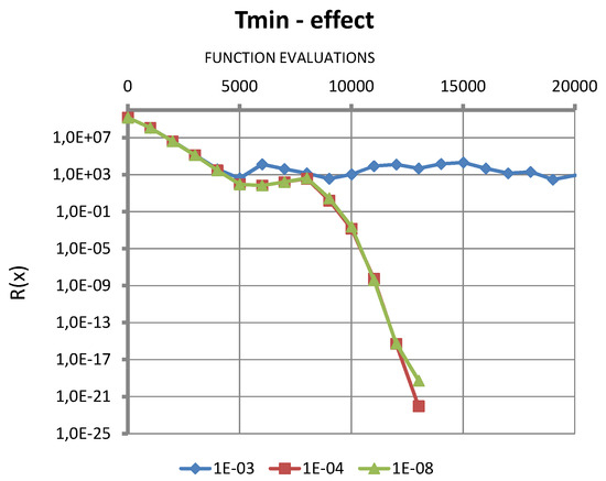
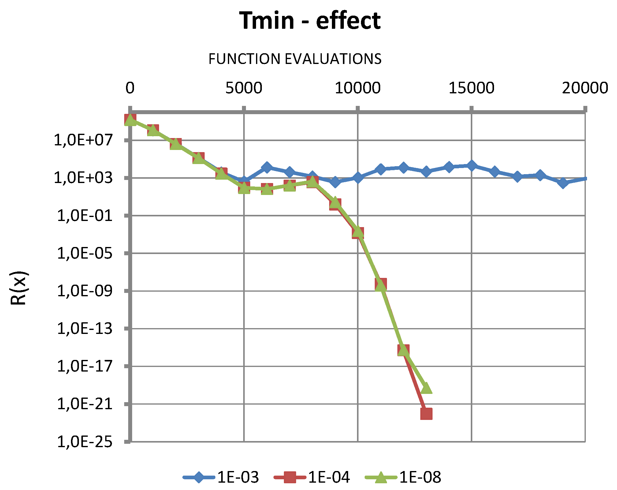
Figure 3 shows the effect of iteration parameter ${\mathit{T}}_{\mathit{min}}$ on the iteration process ($N=1000$). It is clear that too high a value of ${\mathit{T}}_{\mathit{min}}$ has a negative effect on the iteration efficiency. It can be seen in the example that a value $0.001$ causes the iteration process failure, and there is almost no effect with lower values $0.0001\leqq {\mathit{T}}_{\mathit{min}}$.

Figure 3. Effect of the iteration parameter ${\mathit{T}}_{\mathit{min}}$ on the iteration process ($N=1000$).

The suggested procedure may also be repeated without using the classic secant approximates and without updating the previously known Jacobian approximate ${\mathit{S}}_{\mathit{p}}$ as

$$▵{\mathit{x}}_{\mathit{i},\mathit{p}+1+\mathit{h}}={\mathit{x}}_{\mathit{i},\mathit{p}+1+\mathit{h}}^{\mathit{B}}-{\mathit{x}}_{\mathit{i},\mathit{p}+1+\mathit{h}}^{\mathit{A}}={\displaystyle \frac{-{\left({\displaystyle \sum _{\mathit{j}=1}^{\mathit{m}}}\left({\mathit{S}}_{\mathit{i},\mathit{j},\mathit{p}}^{+}{\mathit{f}}_{\mathit{j},\mathit{p}+\mathit{h}}^{\mathit{A}}\right)\right)}^2}{{\displaystyle \sum _{\mathit{j}=1}^{\mathit{m}}}\left({\mathit{S}}_{\mathit{i},\mathit{j},\mathit{p}}^{+}\frac{{\mathit{f}}_{\mathit{j},\mathit{p}+\mathit{h}}^{\mathit{A}}}{{\mathit{t}}_{\mathit{j},\mathit{p}+\mathit{h}}^{\mathit{F}}}\right)}},$$

(77)

where

$${\mathit{t}}_{\mathit{j},\mathit{p}+\mathit{h}}^{\mathit{F}}={\displaystyle \frac{{\mathit{f}}_{\mathit{j},\mathit{p}+1+\mathit{h}}^{\mathit{A}}}{{\mathit{f}}_{\mathit{j},\mathit{p}+\mathit{h}}^{\mathit{A}}}}$$

(78)

$\left(h=1,\dots \right)$ until the new approximates

$${\mathit{x}}_{\mathit{i},\mathit{p}+1+\mathit{h}}^{\mathit{B}}={\mathit{x}}_{\mathit{i},\mathit{p}+1+\mathit{h}}^{\mathit{A}}+▵{\mathit{x}}_{\mathit{i},\mathit{p}+1+\mathrm{h}}$$

(79)

$\left(i=1,\dots ,n\right)$ are sufficiently improved. A numerical example is shown in Table 3 with test function

$$f\left(x\right)=x^3-2x-5$$

(80)

for demonstration purpose. The results indicate linear convergence, with convergence rate $\alpha =1$. $\alpha$ is the computed convergence rate, ${\mathit{N}}_{\mathit{f}}$ is the number of function value evaluations, and $\mathit{L}$ is the mean convergence rate, suggested by Broyden [36] in Table 3.

Table 3. T-Secant iteration with constant Jacobian approximate ${\mathit{S}}_p$ (Equation (77)).

$\mathit{h}$	${\mathit{x}}_{\mathit{p}+\mathit{h}}^{\mathit{A}}$	${\mathit{x}}_{\mathit{p}+\mathit{h}}^{\mathit{B}}$	$\mathit{\Delta }{\mathit{x}}_{\mathit{p}+\mathit{h}}^{\mathit{A}}$	${\mathit{t}}_{\mathit{p}+\mathit{h}}^{\mathit{f}}$	$\mathit{\Delta }{\mathit{x}}_{\mathit{p}+1+\mathit{h}}$	$\left|{\mathit{e}}_{\mathit{p}+1+\mathit{h}}^{\mathit{A}}\right|$	${\mathit{\alpha }}_{\mathit{p}+\mathit{h}}^{\mathit{T}}$	${\mathit{N}}_{\mathit{f}}$	$\mathit{L}$
0	1.700	2.000	0.421	−0.085	0.036	$2.6\times {10}^{-2}$		2	1.23
1	2.121	2.156	−0.036	−0.359	−0.013	$2.2\times {10}^{-2}$		4	0.87
2	2.085	2.072	0.013	−0.342	0.0044	$7.6\times {10}^{-3}$	1.08	6	0.76
3	2.098	2.102	−0.0044	−0.348	−0.0015	$2.7\times {10}^{-3}$	0.97	8	0.70
4	2.093	2.092	0.0015	−0.346	0.00053	$9.2\times {10}^{-4}$	1.01	10	0.67
5	2.0949	2.0955	−0.00053	−0.347	−0.00018	$3.2\times {10}^{-4}$	0.997	12	0.65
6	2.0944	2.0942	0.00018	−0.346	0.000063	$1.1\times {10}^{-4}$	1.001	14	0.63
7	2.0946	2.0947	−0.000063	−0.346	0.000022	$3.8\times {10}^{-5}$	0.9997	16	0.62

5. Algorithm

Let ${\epsilon }^{*}$ be the error bound for termination criterion, and if ${\mathit{x}}^{*}$ is known, then

$${\mathit{e}}_{\mathit{p}}^{\mathit{A}}={\mathit{x}}_{\mathit{p}}^{\mathit{A}}-{\mathit{x}}^{*}$$

(81)

is the error vector of approximate ${\mathit{x}}_{\mathit{p}}^{\mathit{A}}$ in the ${\mathit{p}}^{\mathit{th}}$ iteration with elements ${\mathit{e}}_{\mathit{i},\mathit{p}}^{\mathit{A}}$ $\left(i=1,\dots ,n\right)$. Let the error norm

$${\epsilon }_{\mathit{p}}={\displaystyle \frac{{∥{\mathit{e}}_{\mathit{p}}^{\mathit{A}}∥}_2}{\mathit{n}}}={\displaystyle \frac{\sqrt{{\displaystyle \sum _{\mathit{i}=1}^{\mathit{n}}}{\left({\mathit{e}}_{\mathit{i},\mathit{p}}^{\mathit{A}}\right)}^2}}{\mathit{n}}}$$

(82)

be defined, where ${∥.∥}_2$ is Euclidean norm, and let the iteration be terminated when

$${\epsilon }_{\mathit{p}}<{\epsilon }^{*}$$

(83)

holds. Choose ${\mathit{T}}_{\mathit{min}}$ as the lower bound for $\left|{\mathit{t}}_{\mathit{j},\mathit{p}}^{\mathit{F}}\right|\left(\mathit{j}=1\dots ,\mathit{m}\right)$, and let ${\mathit{f}}_{\mathit{min}}$ be a lower bound for $\left|{\mathit{f}}_{\mathit{j},\mathit{p}}^{\mathit{A}}\right|$ $\left(\mathit{j}=1,\dots ,\mathit{m}\right)$. Let $\mathit{p}=0$, and let the approximate ${\mathit{x}}_{\mathit{p}}^{\mathit{A}}$ and the difference vector $▵{\mathit{x}}_{\mathit{p}}$ be given. Calculate the corresponding function values ${\mathit{f}}_{\mathit{p}}^{\mathit{A}}$ and assure that ${\mathit{f}}_{\mathit{min}}<\left|{\mathit{f}}_{\mathit{j},0}^{\mathit{A}}\right|$ $\left(\mathit{j}=1,\dots ,\mathit{m}\right)$. Iteration constants ${\mathit{f}}_{\mathit{min}}$ and ${\mathit{T}}_{\mathit{min}}$ are necessary to avoid division by zero and to avoid computed values be near the numerical precision.

• Step 1: Generate a set of $\mathit{n}$ additional approximates ${\mathit{x}}_{\mathit{k},\mathit{p}}^{\mathit{B}}$ (Equation (64)) and evaluate function values ${\mathit{f}}_{\mathit{k},\mathit{p}}^{\mathit{B}}$ $\left(\mathit{k}=1,\dots ,\mathit{n}\right)$. Assure that ${\mathit{f}}_{\mathit{min}}<\left|{\mathit{f}}_{\mathit{k},\mathit{j},\mathit{p}}^{\mathit{B}}\right|$ $\left(\mathit{j}=1,\dots ,\mathit{m}\right)$.
• Step 2 (Classic secant update method): Construct the Jacobian approximate matrix ${\mathit{S}}_p$, determine its pseudoinverse ${\mathit{S}}_p^{+}$ [4], calculate ${\mathit{x}}_{\mathit{p}+1}^{\mathit{A}}$ from Equation (40) and ${\epsilon }_p$ from Equation (82).
• Step 3: If ${\epsilon }_p<{\epsilon }^{*}$, then terminate iteration, else continue with Step 4.
• Step 4 (suggested update method): Calculate ${\mathit{f}}_{\mathit{p}+1}^{\mathit{A}}$ (assure that ${\mathit{f}}_{\mathit{min}}<\left|{\mathit{f}}_{\mathit{j},\mathit{p}}^{\mathit{A}}\right|$), ${\mathit{T}}_{\mathit{p}}^{\mathit{F}}$ from Equation (66) and ${\mu }_{\mathit{i}}$ from Equation (74). Let ${\mathit{T}}_{\mathit{min}}<\left|{\mathit{t}}_{\mathit{j},\mathit{p}}^{\mathit{F}}\right|$ and determine ${\mathit{x}}_{\mathit{p}+1}^{\mathit{B}}$ from Equation (75).
• Step 5 : Continue iteration from Step 1 with $\mathit{p}=\mathit{p}+1$, ${\mathit{x}}_{\mathit{p}+1}^{\mathit{A}}$ and ${\mathit{x}}_{\mathit{p}+1}^{\mathit{B}}$.

If ${\mathit{p}}_{\mathit{max}}$ is the number of necessary iterations for satisfying the termination criterion ${\epsilon }_p<{\epsilon }^{*}$ and $\mathit{n}$ is the number of unknowns to be determined, then the suggested update method needs $n+1$ function evaluations in each iterations and altogether

$${\mathit{N}}_{\mathit{f}}={\mathit{p}}_{\mathit{max}}\left(\mathit{n}+1\right)$$

(84)

function evaluations to reach the desired termination criterion. ${\mathit{p}}_{\mathit{max}}$ is dependent on many circumstances, such as the nature of the function $\mathit{f}\left(\mathit{x}\right)$, termination criteria (${\epsilon }^{*}$ or others), the distance of the initial approximate ${\mathit{x}}^{\mathit{A}}$ from the solution ${\mathit{x}}^{*}$, and from the iteration constants ${\mathit{f}}_{\mathit{min}}$ and ${\mathit{T}}_{\mathit{min}}$.

6. Numerical Tests Results

6.1. Single-Variable Test Function

A numerical example is given with a single-variable test function

$$\mathit{f}\left(x\right)=cos\left(x\right)-x,$$

(85)

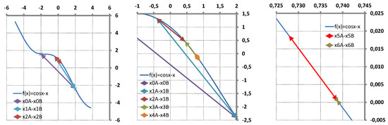
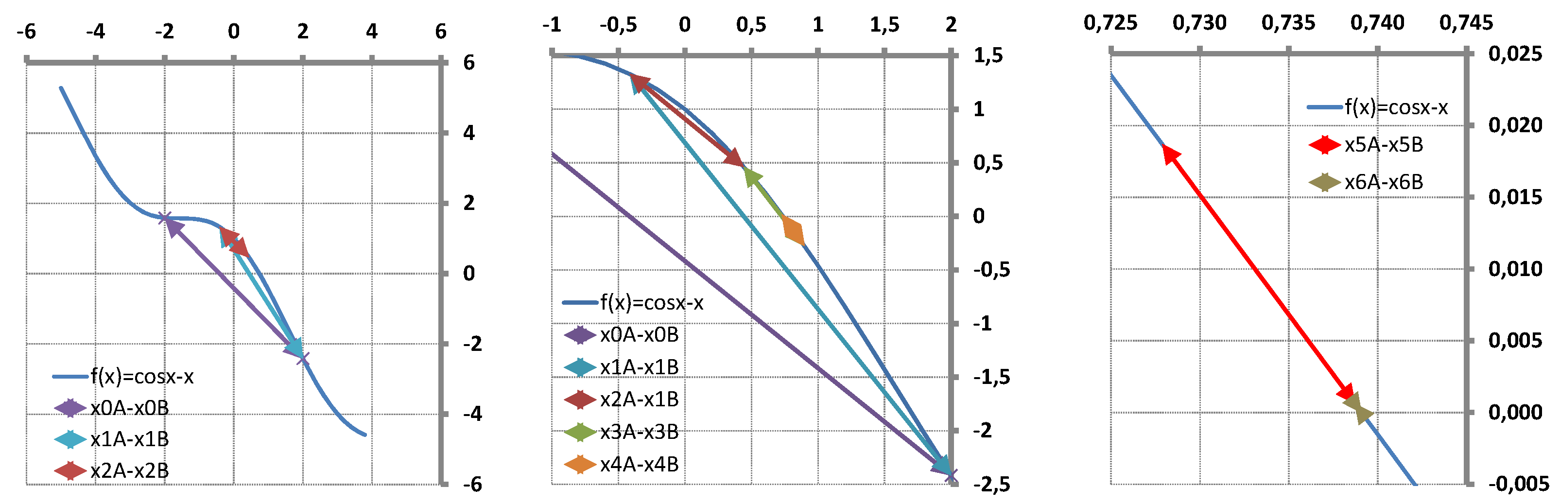
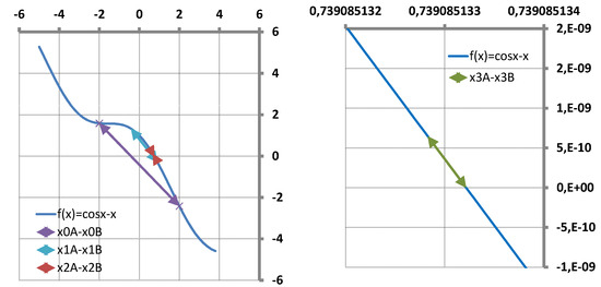
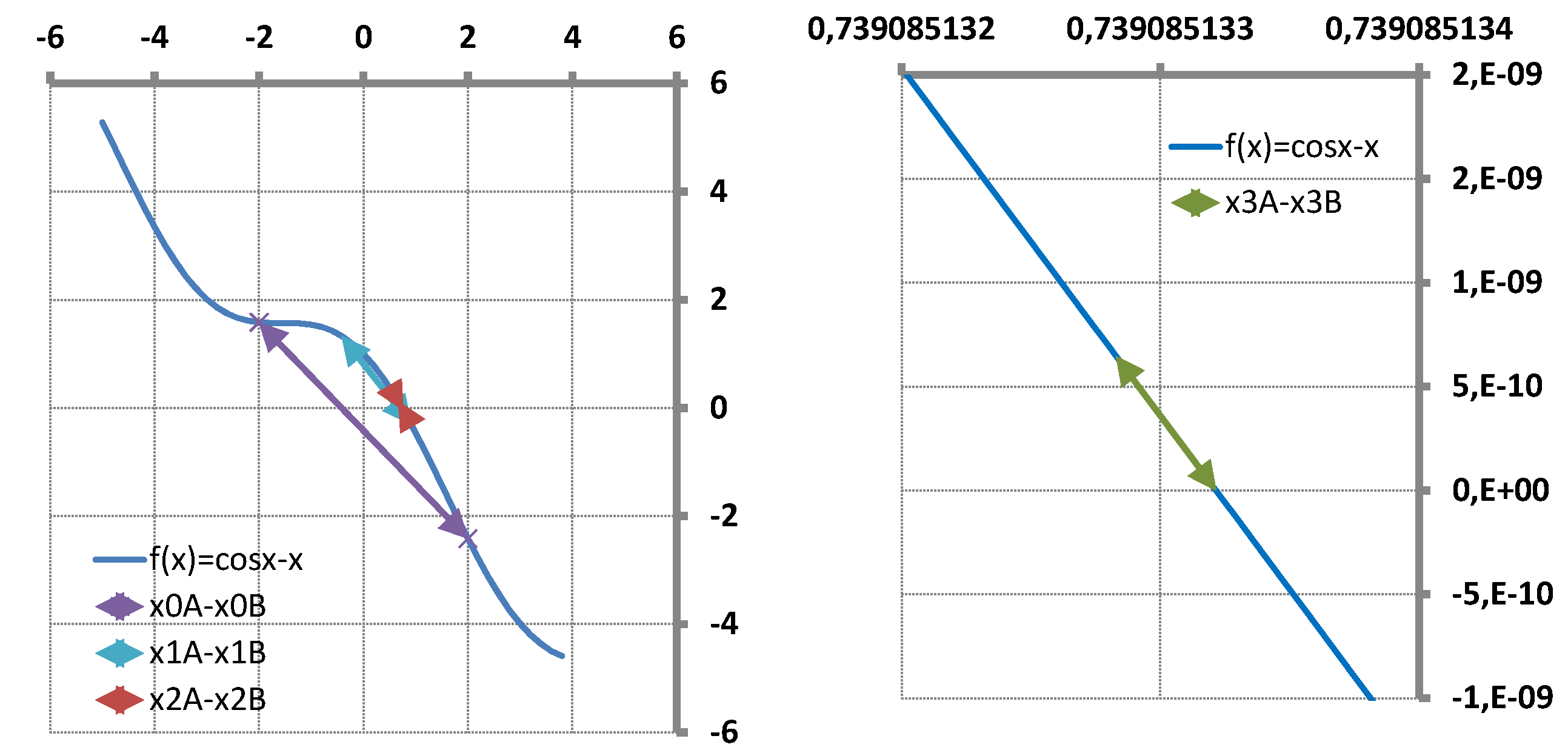
with root ${\mathit{x}}^{*}\cong 0.73908513\dots$ The results of the classic secant iteration process are shown in Table 4 and Figure 4. Iterations were made with initial approximates ${\mathit{x}}_0^{\mathit{A}}=-2.0$ and ${\mathit{x}}_0^{\mathit{B}}=2.0$ $\left(\mathit{p}=0\right)$ providing ${\mathit{f}}_0^{\mathit{A}}=1.584$. The first secant approximate ${\mathit{x}}_1^{\mathit{A}}=-0.416\dots$ is found as the zero of the first secant line ${\mathit{y}}_0\left(\mathit{x}\right)$ providing ${\mathit{f}}_1^{\mathit{A}}=1.331\dots$ $\left(\mathit{p}=1\right)$. The next iteration ($\mathit{p}=2$) will continue with approximate ${\mathit{x}}_2^{\mathit{A}}=0.442\dots$ and with ${\mathit{f}}_2^{\mathit{A}}=0.462\dots$ .

Table 4. Classic secant iterations with test Function (85) (see Figure 4).

$\mathit{p}$	0	1	2	3	4	5	6
$x_p^A$	$-2.000$	$2.000$	$-0.416$	$0.442$	$0.898$	$0.7279$	$0.7387$
$▵{\mathit{x}}_{\mathit{p}}$	$4.000$	$-2.416$	$0.858$	$0.456$	$-0.170$	$0.011$	$3.6\times {10}^{-4}$
${\mathit{f}}_p^A$	$1.584$	$-2.416$	$1.331$	$0.462$	$-0.275$	$0.019$	$6.1\times {10}^{-4}$
$x_{p+1}^A$	$-0.416$	$0.442$	$0.898$	$0.728$	$0.7387$	$0.739086$	$0.739085$
$e_{p+1}^A$	$-1.155$	$-0.297$	$0.159$	$-0.011$	$-0.0004$	$9.1\times {10}^{-7}$	$7.3\times {10}^{-11}$
${\alpha }^{\mathit{S}}$			$0.113$	$15.5$	$0.459$	$4.249$	$1.292$
${\mathit{f}}_{p+1}^A$	$1.331$	$0.462$	$-0.275$	$0.019$	$6.1\times {10}^{-4}$	$1.5\times {10}^{-6}$	$1.2\times {10}^{-10}$

Figure 4. Classic secant iterations with test Function (85) (see Table 4). ($\mathbf{Left}$: ${\mathit{x}}_1^{\mathit{A}}=-0.416\dots$ is the root of ${\mathit{y}}_0\left(\mathit{x}\right)$, then ${\mathit{x}}_2^{\mathit{A}}=0.442\dots$ is the root of ${\mathit{y}}_1\left(\mathit{x}\right)$. $\mathbf{Middle}$: ${\mathit{x}}_3^{\mathit{A}}=0.898\dots$ is the root of ${\mathit{y}}_2\left(\mathit{x}\right)$ and ${\mathit{x}}_4^{\mathit{A}}=0.728\dots$ is the root of ${\mathit{y}}_3\left(\mathit{x}\right)$. $\mathbf{Right}$ : ${\mathit{x}}_5^{\mathit{A}}=0.7387\dots$ is the root of ${\mathit{y}}_4\left(\mathit{x}\right)$ and ${\mathit{x}}_6^{\mathit{A}}=0.739086\dots$ is the root of ${\mathit{y}}_5\left(\mathit{x}\right)$).

The results of the suggested iteration process are shown in Table 5 and Figure 5. Iterations were made with the same initial approximates as in the case of the classic secant iteration, and the first secant approximate ${\mathit{x}}_1^{\mathit{A}}=-0.416\dots$ is found. The first T-secant approximate ${\mathit{x}}_1^{\mathit{B}}=0.915\dots$ is given as the zero of the first hyperbola function ${\mathit{z}}_0\left(\mathit{x}\right)$ (Figure 5, left). Iteration then goes on with approximates ${\mathit{x}}_1^{\mathit{A}}=-0.416\dots$ and ${\mathit{x}}_1^{\mathit{B}}=0.915\dots$ providing ${\mathit{f}}_1^{\mathit{A}}=1.331\dots$ $\left(\mathit{p}=1\right)$, and new approximates ${\mathit{x}}_2^{\mathit{A}}=0.667\dots$ and ${\mathit{x}}_2^{\mathit{B}}=0.764\dots$ as the zeros of the second secant and hyperbola functions ${\mathit{y}}_1\left(\mathit{x}\right)$ and ${\mathit{z}}_1\left(\mathit{x}\right)$ receptively (Figure 5, left). The next iteration ($\mathit{p}=2$) will then continue with approximates ${\mathit{x}}_2^{\mathit{A}}=0.667\dots$ and ${\mathit{x}}_2^{\mathit{B}}=0.764\dots$ and with ${\mathit{f}}_2^{\mathit{A}}=0.119\dots$ and gives ${\mathit{x}}_3^{\mathit{A}}=0.7387\dots$ and ${\mathit{x}}_3^{\mathit{B}}=0.7391\dots$ (Figure 5, right).

Table 5. T-Secant iterations with test Function (85) (see Figure 5).

$\mathit{p}$	0	1	2	3	4
$x_p^A$	$-2.000$	$-0.416$	$0.6668$	$0.7387$	$0.7390851328$
$▵{\mathit{x}}_{\mathit{p}}$	$4.000$	$1.331$	$0.0968$	$4.1\times {10}^{-4}$	$3.9\times {10}^{-10}$
${\mathit{f}}_p^A$	$1.584$	$1.331$	$0.1190$	$6.7\times {10}^{-4}$	$6.5\times {10}^{-10}$
$x_{p+1}^A$	$-0.416$	$0.667$	$0.7387$	$0.7390851328$	$0.7390851332$
$e_{p+1}^A$	$-1.155$	$-0.072$	$-4.0\times {10}^{-4}$	$3.8\times {10}^{-10}$
${\alpha }^{\mathit{TS}}$			$3.210$	$1.874$	$2.668$
${\mathit{f}}_{p+1}^A$	$1.331$	$0.119$	$6.7\times {10}^{-4}$	$6.5\times {10}^{-10}$
${\mathit{t}}_{\mathit{p}}^{\mathit{F}}$	$0.840$	$0.089$	$0.0057$	$9.6\times {10}^{-7}$
$x_{p+1}^B$	$0.915$	$0.764$	$0.7391$	$0.7390851332$

Figure 5. T-Secant iterations with test Function (85) (see Table 5) ($\mathbf{Left}$: ${\mathit{x}}_1^{\mathit{A}}=-0.416\dots$ is the root of ${\mathit{y}}_0\left(\mathit{x}\right)$, ${\mathit{x}}_1^{\mathit{B}}=0.915\dots$ is the root of ${\mathit{z}}_0\left(\mathit{x}\right)$, then ${\mathit{x}}_2^{\mathit{A}}=0.667\dots$ is the root of ${\mathit{y}}_1\left(\mathit{x}\right)$, ${\mathit{x}}_2^{\mathit{B}}=0.764\dots$ is the root of ${\mathit{z}}_1\left(\mathit{x}\right)$. $\mathbf{Right}$: ${\mathit{x}}_3^{\mathit{A}}=0.7387\dots$ is the root of ${\mathit{y}}_2\left(\mathit{x}\right)$, ${\mathit{x}}_3^{\mathit{B}}=0.7391\dots$ is the root of ${\mathit{z}}_2\left(\mathit{x}\right)$).

6.2. Solution of an Inverse Problem

An example is given for an imaginary modeling problem. The modeling of systems on the basis of observed or specified system responses plays a key role in scientific research. A central problem of modeling is to fit a structured mathematical model to available data so that the values of the unknown model parameters are determined providing that the simulated data are as near to the available data as possible. A system response can generally be represented by a “curve” in a two (or three)-dimensional space and can be simulated by a computer program. Parameter identification corresponds to minimizing the distance between observed and simulated system responses. Parameter identification problems can generally be formulated as nonlinear least-squares problems so that some unknown model parameters are determined providing minimal deviation between observed and simulated system responses. Solving nonlinear least-squares problems is often a difficult task, especially if the number of unknowns is high.

A rational system under investigation produces a measurable response to a known measurable external effect. A mathematical model with $\mathit{n}$ unknown parameters $\left(p_1,\dots ,p_n\right)$ simulates the behavior of the system providing response to the same external effect as acted on the system during observation. Let the observed and the simulated system responses be represented by two-dimensional curves and sampled in k discrete points with coordinates ${\mathit{x}}_{\mathit{i}}$ and ${\mathit{y}}_{\mathit{i}}$$\left(i=1,\dots k\right)$. The coordinates of a synthetic observed response were generated as

$$\mathit{x}\left(\mathit{z}\right)=\left(\mathit{a}+\mathit{b}\right)cos\left(\mathit{z}+\alpha \right)-\mathit{c}cos\left({\displaystyle \frac{\mathit{a}+\mathit{b}}{\mathit{b}}}\mathit{z}+\alpha \right)+{\mathit{x}}_{\mathit{0}}$$

(86)

$$\mathit{y}\left(\mathit{z}\right)=\left(\mathit{a}+\mathit{b}\right)sin\left(\mathit{z}+\alpha \right)-\mathit{c}sin\left({\displaystyle \frac{\mathit{a}+\mathit{b}}{\mathit{b}}}\mathit{z}+\alpha \right)+{\mathit{y}}_{\mathit{0}}$$

(87)

(an epicycloid) with parameters ${\mathit{x}}_{\mathit{0}}=10$, $\mathit{y}=8$, $\mathit{a}=4$, $\mathit{b}=2$, $\mathit{c}=3.5$ and $\alpha =1$ and with $0\leqq z\leqq 2\pi$. The parameters

$$\mathit{p}=\left[\begin{array}{ccccc}{\mathit{x}}_{\mathit{0}}& {\mathit{y}}_{\mathit{0}}& \mathit{a}& \mathit{b}& \mathit{c}\end{array}\right]$$

(88)

were considered to be unknown, and the system response was simulated with initial approximate

$$p_0=\left[\begin{array}{ccccc}{\mathit{x}}_{\mathit{0}}& {\mathit{y}}_{\mathit{0}}& \mathit{a}& \mathit{b}& \mathit{c}\end{array}\right]=\left[\begin{array}{ccccc}\mathit{8}& \mathit{11}& \mathit{3}.\mathit{5}& \mathit{2}.\mathit{5}& \mathit{3}\end{array}\right].$$

(89)

The distance between observed and simulated system responses was defined for arbitrary two-dimensional curves. This definition can be extended to $\mathit{n}$ dimensions making a wide range of parameter identification problems possible to formulate. The value of the defined distance is dimensionless, and it expresses the ratio of the area between the system response graphs in a normalized coordinate system to the area of a rectangle with unit area.

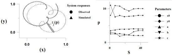
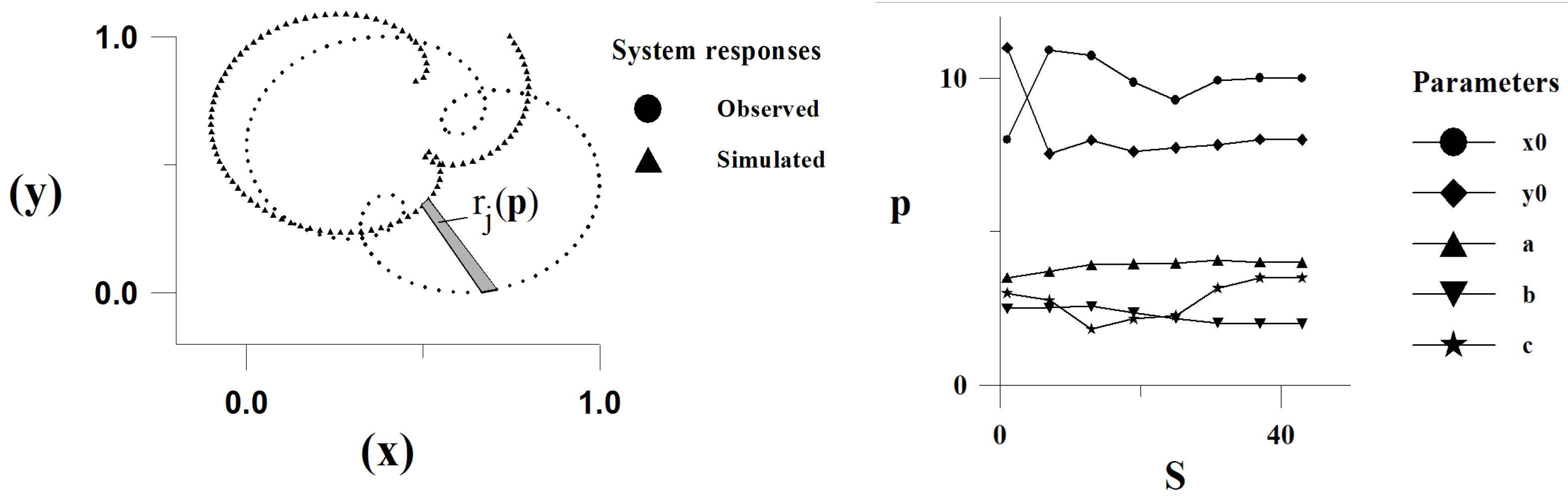
The distance between the observed and simulated system responses was quantified by area $\mathit{D}\left(\mathit{p}\right)$ between the graphs of system responses in a normalized coordinate system. Partial area ${\mathit{r}}_{\mathit{j}}\left(\mathit{p}\right)$ was defined as the area of a quadrangle among the ${\left(j-1\right)}^{th}$ and ${\mathit{j}}^{\mathit{th}}$ division points on the system response graphs $\left(j=1,\dots ,m\right)$, as shown in Figure 6. These division points were selected equidistantly along system response graphs.

Figure 6. Definition of the distance between system responses (left) and variations in parameters through iterations (right).

Thus, parameter identification problems can be formulated as solving a system of nonlinear equations

$$\mathit{r}\left(\mathit{p}\right)=\mathit{0},$$

(90)

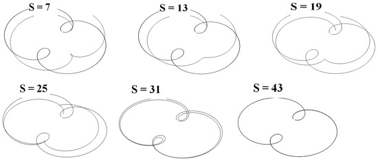
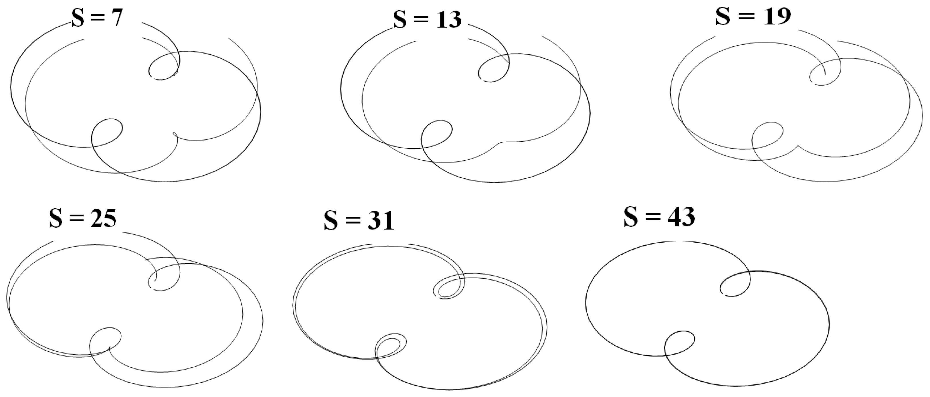
where $\mathit{p}\to \mathit{r}\left(\mathit{p}\right)$, $\mathit{p}\in {\mathbb{R}}^5$, $\mathit{r}:{\mathbb{R}}^5\to {\mathbb{R}}^m$ and $\mathit{r}$ is residual vector with components ${\mathit{r}}_{\mathit{j}}$$\left(j=1,\dots ,m\right)$. The unknown parameters $\mathit{p}$ of an epicycloid (86) and (87) were determined according to the suggested update algorithm. The variation in parameters $\mathit{p}$ through iterations and the observed and simulated system responses for the initial approximate are shown in Figure 6. The observed and simulated system response pairs are shown in Figure 7 7, 13, 19, 25, 31 and 43 simulations ($\mathit{S}$).

Figure 7. Observed and simulated system response pairs after “S” function value evaluations.

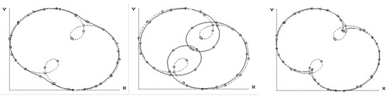
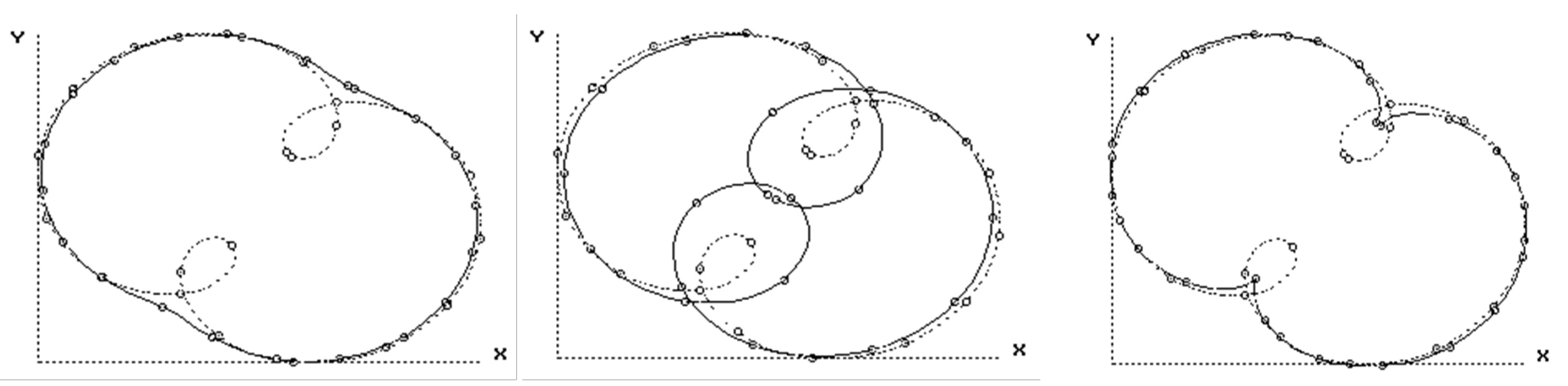
The results of numerical tests with different initial approximates show that the optimal solutions were not reached in all cases. The convergence was especially sensitive for the initial values of parameters $\mathit{a}$, $\mathit{b}$, and $\mathit{c}$. Several local optimal solutions were detected, as shown in Figure 8.

Figure 8. Local optimal solutions.

7. Efficiency

The efficiency of an algorithm for the solution of nonlinear equations is thoroughly discussed by Traub [15], as follows. Let $\beta$ be the order of the iteration sequence such that for the approximate errors ${\mathit{e}}_{\mathit{i}}=x_i-x^{*}$, there exists a nonzero constant $\mathit{C}$ (asymptotic error constant) for which

$${\displaystyle \frac{\left|{\mathit{e}}_{\mathit{i}+1}\right|}{{\left|{\mathit{e}}_{\mathit{i}}\right|}^{\beta }}}\to \mathit{C}.$$

(91)

A natural measure of the information used by an algorithm is the “informational usage” $\mathit{d}$, which is defined as the number of new pieces of information (values of the function and its derivatives) required per iteration (called “horner” by Ostrowski [14]). Then, the efficiency of the algorithm within one iteration can be measured by the “informational efficiency”

$$\mathit{EFF}={\displaystyle \frac{\beta }{\mathit{d}}}.$$

(92)

An alternative definition of efficiency is

$$*\mathit{EFF}={\beta }^{{\displaystyle \frac{1}{\mathit{d}}}},$$

(93)

called “efficiency index” by Ostrowski [14]. Another measure of efficiency, called “computational efficiency”, takes into account the “cost” of calculating different derivatives. The concepts of informational efficiency ($\mathit{EFF}$) and efficiency index ($*\mathit{EFF}$) do not take into account the cost of evaluating $\mathit{f}$ and its derivatives, nor do they take into account the total number of pieces of information needed to achieve a certain accuracy in the root of the function. If $\mathit{f}$ is composed of elementary functions, then the derivatives are also composed of elementary functions; thus, the cost of evaluating the derivatives is merely the cost of combining the elementary functions.

Broyden [36] suggested the mean convergence rate

$$\mathit{L}={\displaystyle \frac{1}{{\mathit{N}}_{\mathit{f}}}}ln{\displaystyle \frac{\mathit{R}\left({\mathit{x}}_0^{\mathit{A}}\right)}{\mathit{R}\left({\mathit{x}}_{{\mathit{p}}_{\mathit{max}}}^{\mathit{A}}\right)}}$$

(94)

as a measure of the efficiency of an algorithm for solving a particular problem, where ${\mathit{N}}_{\mathit{f}}$ is the total number of function evaluations, ${\mathit{x}}_0^{\mathit{A}}$ is the initial approximate, ${\mathit{x}}_{{\mathit{p}}_{\mathit{max}}}^{\mathit{A}}$ is the last approximate to the solution ${\mathit{x}}^{*}$ when the termination criterion is satisfied after ${\mathit{p}}_{\mathit{max}}$ iterations. $\mathit{R}\left(\mathit{x}\right)$ is the Euclidean norm of $\mathit{f}\left(\mathit{x}\right)$.

Zang’s two-step method [29] is similar to the King–Werner method [38,39] with convergence rate $2.414\dots$ [40]. Chen’s [28] and Wang’s [30] three-step methods show asymptotic convergence order $2.732\dots$. Chen’s [28] method requires two functions and one derivative evaluation using a second-order polynomial, proposed in [30] and shows $1.174\dots$ Ostrowski’s [14] efficiency index. Wang’s [30] method requires three functions and two derivative evaluations showing $1.101\dots$ Ostrowski index. Zhang [29] published a finite-difference-based secant method with $2.618\dots$ asymptotic convergence order. Later, Ren [40] showed that Zhang’s [29] method has only a $2.414\dots$ convergence order due to some mistakes in the derivation. Table 6 compares the efficiencies of classic (Rows 1–2: Secant, Newton) and improved algorithms (Rows 3, 5: T-Secant, T-Newton with the suggested full-rank update and from references [28,30]), the T-secant method with constant Jacobian approximate ${\mathit{S}}_{\mathit{p}}$ (row 4: TS-const. ${\mathit{S}}_{\mathit{p}}$, see data in Table 3), and Chen’s [28] and Wang’s [30] methods.

Table 6. Efficiencies of classic and improved algorithms.

	Method	$\mathit{d}$	$\mathit{\beta }$	$\mathit{EFF}$ [15]	$*\mathit{EFF}$ [14]	${\mathit{L}}_{\mathit{max}}$ [36]
1	Secant	1	1.618…	1.618…	1.618…	4.0
2	Newton	2	2.0	1.0	1.414…	3.0
3	T-Secant	2	2.618…	1.309…	1.618…	4.5
4	TS-const. ${\mathit{S}}_{\mathit{p}}$	2	1.0	0.5	1.0	0.6
5	T-Newton	3	3.0	1.0	1.442…	3.0
6	Chen [28]	3	1.618…	0.539…	1.173…	−
7	Wang [30]	5	1.618…	0.323…	1.101…	−

Very limited data are available to compare the performance of the suggested update method (T-Secant) with other classic methods, especially for a large number of unknowns. Efficiency results were given by Broyden [36] for the Rosenbrock function for $\mathit{N}=2$. The calculated convergence rates for the two Broyden method variants [36], for the Powell’s method [41], for the adaptive coordinate descent method [42], and for the Nelder–Mead simplex method [43] were compared with the calculated values for the T-secant method in Table 7 [5]. Rows 1–5 are data from referenced papers, rows 6–8 are T-secant results with the referenced initial approximates, and rows 9–15 are calculated data for $\mathit{N}>2$. If the value of $\mathit{R}\left(\mathit{x}\right)=0$ (for ${\mathit{p}}_{\mathit{max}}$) is zero, then the mean convergence rates ($\mathit{L}$ and ${\mathit{L}}_{\mathit{N}}$) are not countable (zero in the denominator). A substitute value ${10}^{-25}$ was used when $\mathit{R}\left(\mathit{x}\right)=0$ (for ${\mathit{p}}_{\mathit{max}}$) in rows 6, 7, 10, and 13.

Table 7. Calculated values of the mean convergence rates.

	$\mathit{N}$	Method	$\mathit{R}\left({\mathit{x}}_0^{\mathit{A}}\right)$	$\mathit{R}\left({\mathit{x}}_{{\mathit{p}}_{\mathit{max}}}^{\mathit{A}}\right)$	${\mathit{p}}_{\mathit{max}}$	${\mathit{N}}_{\mathit{f}}$	$\mathit{L}$	${\mathit{L}}_{\mathit{N}}$
1	2	Broyden 1. [36]	4.92	$4.7E{-}^{10}$	-	59	0.391	0.78
2	2	Broyden 2. [36]	4.92	$2.6E^{-10}$	-	39	0.607	1.22
3	2	Powell [41]	4.92	$7.0E^{-10}$	-	151	0.150	0.30
4	2	ACD [42]	130.1	$1.0E^{-10}$	-	325	0.086	0.17
5	2	Nelder–Mead [43]	2.00	$1.4E^{-10}$	-	185	0.127	0.25
6	2	T-secant [36,41]	4.92	$1.0E^{-25}$	3	9	6.573	13.15
7	2	T-secant [42]	130.1	$1.0E^{-25}$	3	9	6.937	13.87
8	2	T-secant [43]	2.00	$6.7E^{-15}$	2	6	5.556	11.11
9	3	T-secant	72.72	$1.4E^{-14}$	5	20	1.809	5.43
10	3		32.47	$1.0E^{-25}$	4	16	3.815	11.45
11	5		93.53	$1.3E^{-14}$	8	48	0.760	3.80
12	5		7.19	$5.9E^{-14}$	4	24	1.351	6.76
13	10		202.6	$1.0E^{-25}$	14	154	0.408	4.08
14	200		92.78	$9.0E^{-15}$	10	2010	0.042	8.44
15	1000		212.4	$3.6E^{-13}$	6	6006	0.006	5.66

Results show that the mean convergence rate $\mathit{L}$ (Equation (94)) for $\mathit{N}=2$ is much higher for the T-secant method ($\simeq 5.5-6.9$) than for the other listed methods ($\simeq 0.1-0.6$). However, it is obvious that the mean convergence rate values decrease rapidly with increasing $\mathit{N}$ values (more unknowns need more function evaluations). A modified convergence rate

$${\mathit{L}}_{\mathit{N}}=\mathit{N}\ast \mathit{L}={\displaystyle \frac{\mathit{N}}{{\mathit{N}}_{\mathit{f}}}}ln{\displaystyle \frac{\mathit{R}\left({\mathit{x}}_0^{\mathit{A}}\right)}{\mathit{R}\left({\mathit{x}}_{{\mathit{p}}_{\mathit{max}}}^{\mathit{A}}\right)}}$$

(95)

is suggested to use as an “$\mathit{N}$” independent measure of efficiency (see Table 7). The values of $\mathit{L}$ and ${\mathit{L}}_{\mathit{N}}$ are at least 10 times larger for the T-secant method than for the referenced classic methods for $\mathit{N}=2$ (see Table 7).

The efficiency measures ($\mathit{L}$ and ${\mathit{L}}_{\mathit{N}}$) also depend on the initial conditions (distance of the initial approximate from the optimal solution and termination criterion). Results from a large number of numerical tests indicate an average ${\mathit{L}}_{\mathit{N}}\simeq 7.4$ with a standard deviation of around $3.7$ for the T-secant method, even for large $\mathit{N}$ values.

8. Conclusions

A numerical procedure has been developed for solving an overdetermined system of nonlinear Equation (5). It can be considered both as a discretized Newton method or as a quasi-Newton method with a full-rank update of the Jacobian approximates. Quasi-Newton methods are widely used for solving systems of nonlinear equations when the function derivatives (Jacobian) are not known or difficult to determine. The derivatives (Jacobian) are approximated by divided differences (35), and the system of nonlinear Equation (5) is solved by repeatedly solving systems of linear Equation (43). The new approximate ${\mathit{x}}_{p+1}^A$ is determined from the classic secant equation, and the divided differences are updated according to the secant condition (45). However, the secant condition does not uniquely specify the Jacobian approximate, so the update procedure is not well defined, and further constraints are needed. Different methods offer specific update solutions.

The suggested numerical procedure (“T-Secant” method [5]) provides an unconventional and simple strategy to improve the performance of quasi-Newton iterations by a full-rank update of the Jacobian approximates. It is based on the classic secant linearization and allows a full-rank update of the Jacobian approximates. The classic secant iteration was completed with a new independent approximate ${\mathit{x}}_{p+1}^B$, that was determined from a modified secant Equation (68). A modification was made by a suitably chosen nonuniform scaling transformation. Scaling was made by the difference quotients of the classic secant function value improvements (66), the difference quotients of the desired new iteration stepsizes, and the classic secant stepsizes (67). A new independent approximate ${\mathit{x}}_{p+1}^B$ was determined from the modified secant Equation (68). The solution to the secant equation presented in [5] was based on the Wolfe–Popper procedure [9,10] so that the secant equation was splitted into two equations by introducing an auxiliary variable. The simplified algorithm, presented in the paper, directly solves the secant equation by using the pseudoinverse (71) of the transformed Jacobian approximate (69).

It has been shown that the new T-secant approximate ${\mathit{x}}_{p+1}^B$ will be in the vicinity of the classic secant approximate ${\mathit{x}}_{p+1}^A$ if the classic secant iterates converge to the root of the nonlinear function [5]. The Jacobian approximate was then full-rank updated by constructing new divided differences (Jacobian approximates) from the classic secant and from the T-secant approximates.

It was shown that the iterative procedure possesses superquadratic asymptotic convergence property with convergence rate $\alpha =\phi +1={\phi }^2\simeq \mathbf{2}.\mathbf{618}$ for simple root in a single-variable case ([5]), where $\phi$ is the golden section ratio. The suggested procedure can also be applied to Newton’s method (matrix ${\mathit{S}}_{\mathit{p}}$ corresponds to the Jacobian matrix ${\mathit{J}}_{\mathit{p}}$). Numerical test results indicate that the quadratic convergence ($\alpha =\mathbf{2}$) of Newton’s method increases to cubic ($\alpha =\mathbf{3}$).

The efficiency has been studied in a multi-variable case and compared with other classic rank-one update and line-search methods on the basis of available data. Results show that its efficiency is considerably better than the efficiency of other classic low-rank update methods. The suggested method’s performance was demonstrated by the results of numerical tests with widely used single- and multi-variable benchmark test functions. A Rosenbrock test function was used with up to 1000 variables [5]. The method has also been successfully applied for the solution of different “real-life” inverse problems [6,7,8] on physically nonlinear dynamic systems. Further studies can be carried out on convergence properties in the case of multiple roots and on the efficiency characteristics in cases of more benchmark test functions. The suggested procedure may be used for other applications, especially with a large number of unknowns and when a low number of function evaluations is crucial.

References

- Dennis, J.E., Jr.; Schnabel, R.B. Numerical Methods for Unconstrained Optimization and Nonlinear Equations; Prentice-Hall: Englewood Cliffs, NJ, USA, 1983. [Google Scholar]
- Ortega, J.M.; Rheinboldt, W.C. Iterative Solution of Nonlinear Equations in Several Variables; Academic Press: New York, NY, USA, 1970. [Google Scholar]
- Hegedus, C. Numerical Methods I; ELTE, Faculty of Informatics: Budapest, Hungary, 2015. [Google Scholar]
- Press, W.H.; Flannery, B.P.; Teukolsky, S.A.; Wetterling, W.T. Numerical Recepies; Cambridge University Press: Cambridge, UK, 1986. [Google Scholar]
- Berzi, P. Convergence and Stability Improvement of Quasi-Newton Methods by Full-Rank Update of the Jacobian Approximates. AppliedMath 2024, 4, 143–181. [Google Scholar] [CrossRef] [Scilit]
- Berzi, P.; Beccu, R.; Lundberg, B. Identification of a Percussive Drill Rod Joint from its Response to Stress Wave Loading. Int. J. Impact Eng. 1994, 18, 281–290. [Google Scholar] [CrossRef] [Scilit]
- Berzi, P. Pile-Soil Interaction due to Static and Dynamic Load. In Proceedings of the 13th International Conference on Soil Mechanics and Foundation Engineering, New Delhi, India, 5–10 January 1994; pp. 609–612. [Google Scholar]
- Berzi, P.; Popper, G. Evaluation of dynamic load test results on piles. In Proceedings of the International Symposium on Identification of Nonlinear Mechanical Systems from Dynamic Tests (Euromech 280), Ecully, France, 29–31 October 1991; pp. 121–128. [Google Scholar]
- Popper, G. Numerical method for least square solving of nonlinear equations. Period. Polytech. 1985, 29, 67–69. [Google Scholar]
- Wolfe, P. The Secant Method for Simultaneous Nonlinear Equations. Commun. ACM 1959, 2, 12–13. [Google Scholar] [CrossRef] [Scilit]
- Papakonstantinou, J.M.; Tapia, R.A. Origin and evolution of the secant method in one dimension. Am. Math. Mon. 2013, 120, 500–518. [Google Scholar] [CrossRef] [Scilit]
- Broyden, C.G.; Dennis, J.E.; Mor, J.J. On the local and superlinear convergence of quasi-Newton methods. J. Inst. Math. Appl. 1973, 12, 223–245. [Google Scholar] [CrossRef] [Scilit]
- Dennis, J.E.; Mor, J.J. A characterization of superlinear convergence and its application to quasi-Newton methods. Math. Comput. 1974, 28, 543–560. [Google Scholar] [CrossRef]
- Ostrowski, A.M. Solution of Equations and Systems of Equations; Academic Press: New York, NY, USA, 1966. [Google Scholar]
- Traub, J.F. Iterative Methods for the Solution of Equations, 1st ed.; Prentice-Hall, Inc.: Englewood Cliffs, NJ, USA, 1964. [Google Scholar]
- Weerakoon, S.; Fernando, T.G.I. A variant of Newton’s method with accelerated third-order convergence. Appl. Math. Lett. 2000, 13, 87–93. [Google Scholar] [CrossRef] [Scilit]
- Gerlach, J. Accelerated convergence in Newton’s method. SIAM Rev. 1994, 36, 272–276. [Google Scholar] [CrossRef] [Scilit]
- Homeier, H.H.H. On Newton-type methods with cubic convergence. J. Comput. Appl. Math. 2005, 176, 425–432. [Google Scholar] [CrossRef] [Scilit]
- Kou, J.; Li, Y.; Wang, X. Third-order modification of Newton’s method. J. Comput. Appl. Math. 2007, 205, 1–5. [Google Scholar]
- Kanwar, V.; Sharma, J.R.; Mamta, J. A new family of Secant-like method with super-linear convergence. Appl. Math. Comput. 2005, 171, 104–107. [Google Scholar] [CrossRef] [Scilit]
- Melman, A. Geometry and convergence of Euler’s and Halley’s methods. SIAM Rev. 1997, 39, 728–735. [Google Scholar] [CrossRef] [Scilit]
- Özban, A.Y. Some new variants of Newton’s method. Appl. Math. Letter. 2004, 17, 677–682. [Google Scholar] [CrossRef] [Scilit]
- Scavo, T.R.; Thoo, J.B. On the geometry of Halley’s method. Am. Math. Mon. 1995, 102, 417–426. [Google Scholar] [CrossRef] [Scilit]
- Shaw, S.; Mukhopadhyay, B. An improved regula falsi method for finding simple roots of nonlinear equations. Appl. Math. Comput. 2015, 254, 370–374. [Google Scholar] [CrossRef] [Scilit]
- Muller, D.E. A Method for Solving Algebraic Equations Using an Automatic Computer. Math. Tables Other Aids Comput. 1956, 10, 208–215. [Google Scholar] [CrossRef] [Scilit]
- Thukral, R. A New Secant-type method for solving nonlinear equations. Am. J. Comput. Appl. Math. 2018, 8, 32–36. [Google Scholar]
- Amat, S.; Busquier, S.; Gutiérrez, J.M. Geometric constructions of iterative functions to solve nonlinear equations. J. Comput. Appl. Math. 2003, 157, 197–205. [Google Scholar] [CrossRef] [Scilit]
- Chen, L.; Ma, Y. A new modified King–Werner method for solving nonlinear equations. Comput. Math. Appl. 2011, 62, 3700–3705. [Google Scholar] [CrossRef] [Scilit]
- Zhang, H.; Li, D.-S.; Liu, Y.-Z. A new method of secant-like for nonlinear equations. Commun. Nonlinear Sci. Numer. Simul. 2009, 14, 2923–2927. [Google Scholar]
- Wang, X.; Kou, J.; Gu, C. A new modified secant-like method for solving nonlinear equations. Comput. Math. Appl. 2010, 60, 1633–1638. [Google Scholar] [CrossRef] [Scilit]
- Martínez, J.M. Practical quasi-Newton methods for solving nonlinear systems. J. Comput. Appl. Math. 2000, 124, 97–121. [Google Scholar] [CrossRef] [Scilit]
- Stoer, J.; Bulirsch, R. Introduction to Numerical Analysis; Springer: Berlin/Heidelberg, Germany, 2002. [Google Scholar]
- Birgin, E.G.; Krejic, N.; Martinez, J.M. Globally convergent inexact quasi-Newton methods for solving nonlinear systems. Num. Algorithms 2003, 32, 249–260. [Google Scholar] [CrossRef] [Scilit]
- Dembo, R.S.; Eisenstat, S.C.; Steihaug, T. Inexact Newton methods. SIAM J. Numer. Anal. 1971, 19, 400–408. [Google Scholar] [CrossRef] [Scilit]
- Martinez, J.M.; Qi, L. Inexact Newton methods for solving non-smooth equations. J. Comput. Appl. Math. 1995, 60, 127–145. [Google Scholar] [CrossRef] [Scilit]
- Broyden, C.G. A class of Methods for Solving Nonlinear Simultaneous Equations. Math. Comput. Am. Math. 1965, 19, 577–593. [Google Scholar] [CrossRef]
- Strang, G. Introduction to Linear Algebra, revised international ed.; Wellesley-Cambridge Press: Wellesley, MA, USA, 2005. [Google Scholar]
- King, R.F. Tangent method for nonlinear equations. Numer. Math. 1972, 18, 298–304. [Google Scholar] [CrossRef] [Scilit]
- Werner, W. Über ein Verfarhren der Ordnung 1 + √ 2 zur Nullstellenbestimmung. Numer. Math. 1979, 32, 333–342. [Google Scholar] [CrossRef] [Scilit]
- Ren, H.; Wu, Q.; Bi, W. On convergence of a new secant-like method for solving nonlinear equations. Appl. Math. Comput. 2010, 217, 583–589. [Google Scholar] [CrossRef] [Scilit]
- Powell, M.J.D. An efficient method for finding the minimum of a function of several variables without calculating derivatives. Comput. J. 1964, 7, 155–162. [Google Scholar] [CrossRef] [Scilit]
- Loshchilov, I.; Schoenauer, M.; Sebag, M. Adaptive Coordinate Descent. In Proceedings of the Genetic and Evolutionary Computation Conference (GECCO), Dublin, Ireland, 12–16 July 2011; ACM Press: New York, NY, USA, 2011; pp. 885–892. [Google Scholar]
- Nelder, J.A.; Mead, R. A simplex method for function minimization. Comput. J. 1965, 7, 308–313. [Google Scholar] [CrossRef] [Scilit]
Disclaimer/Publisher’s Note: The statements, opinions and data contained in all publications are solely those of the individual author(s) and contributor(s) and not of MDPI and/or the editor(s). MDPI and/or the editor(s) disclaim responsibility for any injury to people or property resulting from any ideas, methods, instructions or products referred to in the content. |
© 2025 by the author. Licensee MDPI, Basel, Switzerland. This article is an open access article distributed under the terms and conditions of the Creative Commons Attribution (CC BY) license (https://creativecommons.org/licenses/by/4.0/).