


Abstract
Coastal zones are subject to a range of natural and anthropogenic processes that result in coastal erosion and accretion, threatening essential infrastructure and straining livelihoods. Analysis of shoreline changes is thus crucial for informing coastal zone planning and management to avert the ramifications of erosion and accretion. Despite a range of literature examining coastline changes worldwide, there is a paucity of literature focusing on Southern Africa, particularly within small harbours. The paper, therefore, aims to analyse shoreline changes at four small harbour zones along the Atlantic Ocean in the Western Cape province, South Africa, over the period from 1985 to 2025. To acquire an accurate shoreline position, four spectral criteria were applied simultaneously: the Automated Water Extraction Index (AWEI), the Modified Normalised Difference Water Index (MNDWI), the Normalised Difference Vegetation Index (NDVI), and the Near Infrared (NIR). Four statistics were then used to measure shoreline changes in the USGS Digital Shoreline Analysis System (DSAS): Net Shoreline Movement (NSM), Shoreline Change Envelope (SCE), End Point Rate (EPR), and Weighted Linear Regression (WLR). Considerable variability was observed within and among the four small harbour study areas, with several erosion and accretion hotspots identified. The 20-year forecast indicated that future shoreline positions would largely maintain the 2025 curvature. Although the study did not reveal significant threats, authorities are encouraged to pay particular attention to erosion and accretion hotspots through appropriate mitigation and adaptation efforts.
1. Introduction
The coastline or shoreline—the zone where a significant water body and land meet—is a critical economic and strategic resource [1], an important ecological space [2], and a tourism asset [3], with millions of people residing within the shoreline environs globally [4,5,6]. Although the terms coastline and shoreline are often used synonymously, deliberately or inadvertently, in the literature [7], subtle distinctions exist between the two. In essence, the shoreline is more temporally variable than the coastline [8], reflecting the dynamic nature of the land-water interface. In this regard, wherever possible, the current study uses the term shoreline rather than coastline, while recognising the need to preserve the terminology used in the cited works to avoid misrepresenting their original intended meaning.
In light of their ecological, tourism, and human settlement functions mentioned above, coastal areas have become urbanised, with the construction of various infrastructure, such as buildings and transport networks, to support different sectors of the economy, ranging from fishing, processing, trade, and tourism [9]. Amid these developments, shorelines are classified into two primary categories: natural and artificial [10]. Natural shorelines result from long-term interactions between sea and land, organically forming a natural boundary between them. With various sub-categories, these shorelines have a particularly meandering morphology. On the contrary, with a distinctively regular geometry, artificial shorelines consist of permanent human-made structures at the land-water interface, such as berms, docks, jetties, and other associated infrastructure [11].
Coasts are highly sensitive and dynamic zones affected by various natural and anthropogenic processes [12,13]. These processes contribute to continuous changes in the shoreline [14], which can be categorised into erosion (retreating towards the land) and accretion (extending seaward) [13]. Reflecting the complex interplay between economic development and ecological changes of the shoreline [15], erosion and accretion pose the risk of damaging essential infrastructure, exerting economic stress, and consequently straining the livelihoods of coastal zone communities [16,17]. Shoreline changes also lead to habitat destruction and a loss of coastal ecosystems [18,19]. As coastal erosion and accretion are largely irreversible processes [17], close monitoring of shoreline changes is crucial for well-informed coastal planning and management [12], including the formulation of mitigation and adaptation strategies [16]. Analysis of shorelines, therefore, not only enhances understanding of the mechanisms driving coastal changes but also informs the development of coastal zone management plans and regulations [20]. Mao et al. [21] add that understanding the historical patterns, trends, and magnitude of shoreline evolution is also essential for predicting future changes at the land-water interface.
Against this backdrop, a range of empirical literature has examined changes in various coastal environments worldwide. These coastal settings include islands [12,14,16], basins [22], lagoons [23], marinas [24], estuaries [25], fishing ports [26], and other various coastal zones. Evidently, most of the literature has focused on Asia, particularly China [11,15,27,28,29,30,31,32,33,34]. Additionally, in their literature review paper, Rahman, Crawford and Islam [5] found that most of the literature on shoreline-related topics was published in the United States of America, followed by India and Spain. However, relatively few studies have focused on the African continent, including North and West African countries such as Egypt [35], Algeria [26], Gambia [19], and Morocco [36,37]; as well as South Africa [38].
Despite insights from studies in various coastal settings and geographical contexts mentioned above, there is a relative paucity of literature on: firstly, shoreline changes within the Southern African context; secondly, shoreline changes experienced at small harbour areas. Compared to large commercial and container ports, Gomez et al. [17] note that small harbours are crucial because of the local populace’s dependence on fishing and agricultural activities. This dependence makes the communities particularly susceptible to shoreline changes that can potentially threaten their livelihoods [17]; and thirdly, as highlighted in the literature review section, there is a need for more research employing a multi-criteria approach to improve shoreline extraction.
To address the literature gap outlined above, the present study aims to analyse shoreline changes of small harbour zones along the Atlantic coast of the Western Cape province of South Africa. Specific objectives of the study are to:
- Extract the Atlantic coast shoreline and analyse changes at the small harbour areas between 1985 and 2025, at 10-year intervals;
- Forecast the shoreline changes at the small harbour areas along the Atlantic coast between 2025 and 2045.
The paper is structured as follows: Section 2 presents a literature review focusing specifically on the methods used in the existing studies. Section 3 introduces the study area. Section 4 provides an outline of the research methods employed. Section 5 presents the findings, followed by the discussion in Section 6. Section 7 concludes the paper.
2. Literature Review
This section presents the literature on extracting, calculating, and predicting shoreline changes, intended to inform the methods used in the paper. The literature was searched in the Academic Search Premier (EBSCO) database using the keyword sieve “coastline” AND “evolution” OR “change”. Conducted in March 2026, the search focused on peer-reviewed journal articles published between 2021 and 2026 and written in English. Fifty relevant articles were identified through the database search. That number was considered a saturation point, as no literature employing distinctly different techniques was being identified at that stage. The database search was supplemented with backward snowballing, particularly to clarify the origins or further details on certain techniques. The process involved tracing relevant citations from the initially identified studies [39]. Snowballing also targeted relevant literature review studies, including Rahman, Crawford and Islam [5], Mishra et al. [6] and Apostolopoulos and Nikolakopoulous [7]. Overall, a combination of the database search and snowballing yielded 65 articles used for the review presented herein.
2.1. Coastline Extraction Methods
The high-water line is commonly used as a shoreline indicator because it is easily visible in satellite images [40]. It represents the land-water interface under normal tidal conditions and is often distinguishable by variations in moisture content, sediment colour, or vegetation. While other indicators, such as the mean high-water line or vegetation lines, are used in certain coastal environments, the high-water line is typically preferred due to its ease of detection and consistency across datasets [41]. Other authors have utilised the high-tide line [42], the instantaneous water line, and the edge of vegetation as shoreline proxies [26]. Amid the plethora of shoreline proxies, the choice of an appropriate indicator primarily depends on the study’s objectives, data quality and availability, and the study area’s specific conditions [41].
Against the prevailing broad view of the land-water interface as a representation of the coastline [12,24,28,31], various methods and techniques have been employed in the literature to extract the coastline. The choice of coastline extraction method forms the critical step in analysing and monitoring coastline change [43]. The appropriate methods revolve around in situ surveys, aerial photography, and remote sensing [12], as overviewed hereunder.
2.1.1. In Situ Methods
Several studies have used traditional in situ methods to delineate the shoreline. For instance, in analysing four study areas in Spain, among other methods, da Silva et al. [44] utilised topobathymetric data and monitored selected beaches twice a year between 2007 and 2015. Jiang et al. [45] also used in situ-measured coastline position data along the Danube Delta on the Romanian coast. Relatedly, in analysing the shoreline of the Tamil coast in India, Dhananjayan et al. [20] collected field data using the global positioning system, with a spatial accuracy of 15 mm. Although in-situ methods offer highly accurate coastline data, as evidenced by the work of Dhananjayan et al. [20], they are particularly costly, labour-intensive, tedious, and consequently have limited spatial and temporal coverage [12,26,46,47,48,49].
2.1.2. Aerial Photography and Remote Sensing
To address the cost and spatial coverage challenges of in situ methods, aerial photography provides detailed coverage of coastal areas [12]. For instance, in the analysis of changes on the Tahaddart coast, Morocco, El Habti et al. [50] used aerial photography to select a reference line and digitise the coastline. However, aerial photography sometimes lacks adequate resolution and is infrequently acquired in financially constrained territories [40].
To overcome the constraints of aerial photography, remote sensing has been employed as a viable alternative, influenced by the increasing availability of satellite imagery, improvements in satellite sensor resolution, and the advancements in geographic data analysis tools, such as Geographic Information Systems (GIS) and image processing techniques [12,51]. Remote sensing technology, therefore, provides quick analysis and enables the exploration of historical shoreline positions [52]. It also provides global coverage, repeatable observations, and a longer temporal span for analysis [53].
The use of various remote sensing water index methods to differentiate water and land has particularly gained popularity due to their automation, user-friendliness, cost-effectiveness [14], and overall effectiveness [53]. Water indices are essentially employed to categorise pixels in imagery into binary classes: water and no-water [54]. The indices used in coastline studies include the Normalised Difference Vegetation Index (NDVI), the Normalised Difference Water Index (NDWI), the Modified Normalised Difference Water Index (MNDWI), the Augmented Normalised Difference Water Index (ANDWI), and the Automated Water Extraction Index (AWEI). Each of these indices varies in effectiveness and accuracy across different coastal environments [55].
The NDVI takes advantage of the reflectance properties of surfaces whereby features with higher near-infrared reflectance and lower red reflectance (such as vegetation) are augmented, while those with low red reflectance and very low NIR reflectance (such as water) are suppressed [56]. In this regard, the NDVI is useful for distinguishing land pixels from water pixels and, accordingly, for distinguishing between water and land. The NDVI values range from −1 to +1. A very low NDVI value (0.1 or lower) indicates barren surfaces like rock or sand. Moderate NDVI values (between 0.2 and 0.3) are typical of shrublands and grasslands, whereas high values (greater than 0.6) are related to dense forests. Bare soil typically has NDVI values close to zero, while negative NDVI values represent water [12,57].
Based on principles similar to those used to derive the NDVI, the NDWI was developed primarily to delineate open water features and to enhance their presence in imagery while at the same time eliminating soil and vegetation features [56]. In the NDWI, water features have positive values, while soil and terrestrial vegetation have zero or negative values [56]. Dahmani et al. [26] argue that the NDWI is effective in distinguishing land from sea due to the high absorption of electromagnetic radiation by water surfaces. However, when applied in urban areas, NDWI-derived results often include built-up features, leading to a larger surface area of the extracted water bodies, but with a significantly reduced accuracy [15,49].
Given the limitations noted above, the MNDWI serves as an improved version of the NDWI [15,49]. Its values also range between −1 and +1, with increasing positive values indicating water surfaces and decreasing and negative values representing non-water features such as built-up land, vegetation, and soil [14]. The MNDWI particularly demonstrates higher accuracy in extracting water bodies within urban areas than the NDWI [15].
Another index, the ANDWI, is based on spectral reflectance in the visible (blue, green, red) and infrared bands (NIR, SWIR1, SWIR2) to augment the contrast between water and other features [55]. The ANDWI is particularly understood to perform better than the MNDWI by removing noise from dark vegetation. It can also accurately classify water concealed by dust storms and suppress noise from rooftops in urban areas [58].
Representing another improved index, the AWEI was conceptualised to amplify the contrast between water and dark surfaces [59]. The AWEI comprises two indices: AWEInsh and AWEIsh. On the one hand, AWEInsh is designed to remove non-water pixels, including dark built surfaces in areas with urban background. On the other, AWEIsh is intended for further accuracy enhancement by eliminating shadow pixels that AWEInsh may not effectively remove [59]. Therefore, the AWEI can significantly reduce misinterpretations of water features [59,60]. Feyisa et al. [59] reiterate that, with higher accuracy than other indices, such as the MNDWI, the AWEI provides an enhanced water index, especially for extracting water features in settings where noisy results are expected due to built-up structures and shadows.
The Tasselled cap transformation, which can be traced to the pioneering work of Kauth and Thomas [61], is a related technique used for extracting the shoreline. It converts the original satellite image into three bands [14,62]. The first two, the brightness and greenness bands, are used to gauge soil brightness and vegetation, respectively. The third, the wetness band, is considered an indicator of soil moisture, water, and other wet attributes. Land and water bodies are then separated by reclassifying the wetness band [14]. For instance, Kassouk et al. [63] applied Tasselled cap analysis to extract the shoreline of the northern Tunisian coast.
To further enhance the accuracy of coastline extraction processes, numerous studies apply thresholding methods to classify ‘water’ and ‘non-water’ from the indices described above, the most common of which is the Otsu method [51,55]. This is an algorithm introduced in the seminal work of Otsu [64] to distinguish water from land, using a threshold selection method. The central idea of this method is to select a suitable threshold and then use the maximum value in cluster variances to separate the background and the aimed feature [65]. The Otsu method categorises the pixels of a grayscale image into binary classes (water and land) in such a way that the intra-class spreading is minimised [66].
2.1.3. Coastline Correction Methods
Despite the usefulness of the water indices and related coastline-extraction techniques overviewed above, environmental variables such as tides and storms can potentially introduce errors in coastline extraction [51]. To address this issue, some researchers correct instantaneous waterlines extracted from satellite imagery by using DEM-derived coastal slopes [67]. For instance, in the spatio-temporal analysis of coastline changes in Laizhou Bay, China, after combining the MNDWI with the Otsu algorithm to extract the instantaneous water line, Mu et al. [27] performed a tidal correction to determine the actual coastline position. Coastline correction methods, however, face limitations in areas lacking in situ tidal information, as simulated data can introduce uncertainties that may decrease confidence in the corrected coastlines [53].
2.1.4. Visual Interpretation
Against the backdrop of the various water indices discussed earlier in the paper, other studies rely on visual interpretation and manual coastline digitisation [68]. Visual image interpretation utilises the human ability to examine the content of satellite images. This examination combines spectral data from the image with contextual information about the study area to identify and classify specific features [69]. Consequently, knowledge of the various object classes in the image aids the interpretation of coastal zones and provides information for visual coastline detection [54,70]. For instance, in preparation for the spatial and temporal analysis of the Yellow River Delta coastline in China, Li et al. [29] visually interpreted satellite imagery to extract the coastline. Also, in analysing the shoreline trends of beaches along the island of Sardinia, in the Western Mediterranean Sea, Simeone et al. [71] manually digitised shorelines at a scale of 1:2500, using dry/wet proxies identifiable in the imagery. Similarly, Da Silva et al. [24] manually digitised the coastline, aligning it with visible features in the imagery, wherein the IWL was interpreted as the visible dry/wet line. Despite the acceptance of manual digitisation, Li et al. [29] advise that, to avoid inadvertent inconsistencies in interpretation arising from potential human subjectivity, a single person should ideally extract the entire coastline for a particular study area.
2.2. Calculating Shoreline Changes
Once a shoreline is extracted using the techniques described in Section 2.1.2 and corrected where required, the most common approaches for measuring shoreline change are cartographical and statistical [22]. Standard statistical approaches include the Linear Regression Rate (LRR) and the Net Shoreline Movement (NSM). The LRR calculates the rate of change by fitting the least squares regression line to the shoreline points, while the NSM estimates the actual distance between the oldest and youngest shoreline [13,72]. Moving from standard approaches, other authors calculate what they term the coastline change degree index, which denotes the percentage change of the coastline length within the selected study area relative to the total length [34].
As emphasised by Wang et al. [45], the commonly used software for analysing shoreline changes is the USGS Digital Shoreline Analysis System (DSAS). Establishing the reference line/baseline is a crucial step in the DSAS analysis [46]. Thereafter, the system generates profiles of coastline datasets from different years, facilitating efficient analysis of coastline changes [53]. The DSAS’s ability to process multi-temporal data and efficiently produce consistent, reliable, and reproducible output makes it particularly suitable for long-term shoreline change analyses [41]. Showing its popularity, a multitude of shoreline studies used the DSAS [9,13,14,16,17,22,24,25,33,41,46,47,48,53,60,63,65,71,73].
2.3. Data Required for Shoreline Extraction and Analysis
Shoreline extraction and analysis require datasets with extensive spatial coverage and sufficient detail to accurately capture changes [45]. Notably, various data sources can yield different statistical values, even when captured at the same location. Such differences can be primarily attributable to the data’s spatial resolution [60].
In light of the various shoreline extraction and analysis techniques discussed earlier in the paper, the data used in shoreline studies are similarly diverse and include the following: aerial photography [24,25]; Google Earth Pro satellite images [19]; sentinel-2 imagery [12,25]; Landsat imagery [13,14,15,16,17,63,74]; a combination of Landsat and Sentinel [27,75,76]; a combination of Landsat and MODIS [77]; and OpenStreetMap shorelines [21]. Among these diverse sources, Landsat is the most used remote sensing dataset [65]. Khakhim et al. [60] assert that it is one of the readily available datasets with an extensive backward time constellation. However, with a resolution of 30 m, Landsat imagery cannot accurately distinguish objects smaller than 30 m. Also, with this resolution, using Landsat imagery could result in less accurate projections of future coastline [60].
2.4. Predicting Future Shoreline
Although effective in decision-making and long-term planning for coastal zones, determining future shoreline positions is a difficult task [13] to fulfil manually. Hence, most of the literature uses either the DSAS or LITLINE model, or a combination of the two, for shoreline prediction. The LITLINE model assumes a constant cross-shore profile during erosion and accretion. It simulates coastline evolution using time-series wave input and coastline alignment data [41]. Other studies have used the Kalman filter model to predict shoreline evolution [13,27], either as a standalone or embedded in the DSAS. The Kalman filter is a statistically based forecasting tool that combines historical and derived shoreline positions to predict future shoreline positions [13,73]. Given that the filter yields future estimates or projections based on previous data, it is a useful predictive function that can forecast shoreline positions decades from the baseline year [60].
2.5. Duration of Analyses
Reflecting wide temporal diversity, the various durations employed in shoreline change analyses include, for example, five years [12]; eight years [26]; nine years [17]; 15 years [16]; 19 years [14,15]; 23 years [60]; 38 years [27,63]; 48 years [13]; 53 years [25]; and 100 years [78]. Apostolopoulos and Nikolakopoulos [7] categorise shoreline changes with reference to time in four classes, namely short (less than 10 years), medium (between 10 and 30 years), long (between 30 and 70 years) and very long-term (longer than 70 years). For predicting future shoreline positions, timeframes can range from eight years [27] to 50 years [36].
2.6. Lessons from the Literature
The literature reviewed in this section provided a comprehensive overview of the methods, techniques, and approaches used in shoreline-related studies to ensure that the paper’s methodological direction is well informed and sound. The following main lessons are drawn from the literature:
- Amid the different shoreline indicators influenced by the specific study objectives and contexts, the land-water interface is accepted as a standard representation of the shoreline;
- There is no standard duration used in the analysis of shoreline changes or in predicting future shoreline positions. The duration is informed by the specific study’s objectives, context, and data availability;
- Despite its resolution limitations, Landsat is the most used dataset for extracting and analysing shoreline changes and projecting future shoreline positions;
- Different water indices have distinct strengths and limitations, and varying levels of effectiveness in water extraction for different study areas. Instead of selecting a single index, there is a need for more research that employs a multi-criteria approach to improve shoreline extraction, drawing on the strengths of each index;
- The DSAS is the most used software for analysing shoreline changes and predicting future shoreline positions.
3. Study Area
This article analyses the shoreline of small harbour zones along the Atlantic Ocean in the Western Cape province of South Africa. In addition to the Port of Cape Town, the Atlantic coast accommodates five small fishing harbours, proclaimed in accordance with the Marine Living Resources Act [79]. These are Laaiplek, Lambert’s Bay, St. Helena Bay, Saldanha Bay, and Pepper Bay. However, the latter two are operationally regarded as one functional harbour, implying that four study areas, not five, are analysed in the paper (Figure 1). Small fishing harbours are a crucial component of South Africa’s Operation Phakisa, which is based on the fundamental premise that oceans are natural capital to be harnessed for local economic development and the benefit of small-scale fishers [80]. Monitoring the shorelines of small harbours is therefore important to ensure their sustainability and, in turn, the protection of the livelihoods dependent on harbour access.
Figure 1.
Locality.
4. Materials and Methods
4.1. Data Acquisition and Pre-Processing
The study analysed the shoreline evolution of four small harbour zones over 40 years, using 1985, 1995, 2005, 2015, and 2025 as the intervals. For each decade, a five-year observation window was established to ensure high data density and mitigate seasonal anomalies. The datasets used in the study are listed in Table 1, and the pre-processing and analysis employed are graphically depicted in Figure 2.
Table 1.
Data sources.
Figure 2.
Flow diagram.
A multi-index automated shoreline extraction methodology followed a three-stage pipeline, wherein images with cloud cover exceeding 40 percent were filtered out. The collection was normalised using the Landsat Collection 2 radiometric scaling factors (Digital Numbers (DN) × 0.0000275 − 0.2). The cloud pixels were then removed using the Quality Assessment band (QA_PIXEL). For the 2005 Landsat 7 collection, data gaps originating from the Scan Line Corrector failure (SLC-off) were masked out, retaining only valid observation pixels to ensure that subsequent calculations were not biased.
4.2. Multi-Index Water Index
To obtain an accurate shoreline by separating seawater from reflective beach sand, dark intertidal zones, and coastal vegetation, a multi-index intersection model, involving simultaneous application of four spectral criteria, was implemented. The AWEI was computed to maximise the contrast between water and dark land surfaces while suppressing background noise. A strict threshold of AWEI > 0.05 was enforced. This threshold was formulated to suppress shadows that could come from urban structures, terrain, and other features that often confuse other water indices. The MNDWI, which separates open water from saturated soils and wet beach sand, used a threshold of MNDWI > 0.1. The NDVI was applied with a threshold of NDVI < 0.1 to mask out dense coastal vegetation. A near-Infrared (NIR) threshold was set to NIR < 0.1 to exploit the high absorption of water bodies in the near-infrared spectrum, ensuring that deep boundaries were captured. Pixels were classified as water only if they satisfied all four criteria concurrently. The method used the indices simultaneously to extract the water boundary, and the equation was as follows:
4.3. Stabilisation and Reducer Logic
To establish a consistent land-water boundary, a temporal stabilisation technique was employed to mitigate the influence of variables such as tidal changes, wave run-ups, and coastal spray. Binary water masks were generated using a per-pixel reducer to determine the relative frequency of water presence. A permanent water surface was defined using a 60 percent frequency threshold. This means only pixels covered by water at least 60 percent of the time were used. This cutoff ignored temporary changes like low tides or crashing waves and ensured a reliable line representing the land-sea boundary.
The calculations above were performed in Google Earth Engine (GEE). The generated land-water boundary was exported to Quantum Geographic Information System (QGIS) software version 3.40.14, where it was further processed and cleaned. The binary mask of water-land was converted into a polygon, and the boundary between water and land was determined as the shoreline. The shorelines were smoothed to avoid pixelation/zigzagging, since they were generated from a raster mask. A baseline between 50 m and 150 m offshore and parallel to the shorelines was generated for each set of shorelines. The baseline and shorelines were exported from QGIS to the DSAS and used to generate transects, shoreline statistics, and shoreline forecasts.
4.4. Statistics for Measuring Shoreline Change
The statistics calculated are the Net Shoreline Movement (NSM), Shoreline Change Envelope (SCE), End Point Rate (EPR), and Weighted Linear Regression (WLR). As outlined by Himmelstoss et al. [72], the NSM and SCE measure the change in distance in meters (m) between shorelines, whereas the EPR and WLR measure the rate of this change between shorelines. All these measurements determine whether the shoreline is eroding, accreting, or remaining stable over time. The NSM measures the directional distance between the oldest and newest shorelines [72], in this case, the distance between the 1985 and 2025 shorelines. Negative distance indicates erosion, positive distance represents accretion, and zero means stability. The SCE measures the largest absolute distance between all shorelines that a transect intersects. The value is always positive, starting from zero. The EPR is obtained by dividing the NSM by the time between the oldest and newest shorelines. Lastly, the WLR is generated from the Linear Regression Rate (LRR), which is obtained by fitting a line through shoreline points intersected by each transect. The WLR takes the LRR and places more weight on data points that have lower uncertainty and penalises those with higher uncertainty [72]. The equations for these statistics are as follows:
where:
—length of years and distances
—weighted mean of years
—weighted mean of distances
—ith year
ith distance
—ith weight
where:
n—length of years
—mean of years
—mean of distances
— year
—ith distance
4.5. Uncertainty
Remote-sensed shoreline extraction inherently contains a level of uncertainty, due to multiple factors, such as environmental dynamics, measurement constraints, effects of tides on shoreline position, sensor limitations, and human errors [30]. Automated shoreline extraction at coarse multispectral satellite resolution (30 m) particularly introduces complex sub-pixel mixtures, especially within highly water-saturated areas along the water-land boundary [81].
To quantify the uncertainty of the shorelines, the error assessment was executed in GEE. These uncertainties were derived directly from sensor specifications, spatial processing, and satellite image metadata across five decadal periods (1985, 1995, 2005, 2015, and 2025).
Following the Root Sum of Squares (RSS) framework adapted for automated satellite-derived shorelines [68], the total positional uncertainty was calculated as follows:
where:
(Georeferencing Error): derived using the USGS Tier 1 geometric calibration metric. This measures how accurately each satellite image aligns with its true spatial position on the ground. The measurement was done for each target decadal year, using a four-year window across Landsat 5, 7, 8, and 9 collections. It is automatically calculated by taking the GEOMETRIC_RMSE_MODEL metadata provided by the USGS.
(Pixel Resolution Error): Accounts for spatial sampling limits. The GEE script’s spectral thresholding performs sub-pixel interpolation. This allows the error to move below the Landsat nominal error of 30 m to a range of ±25 m to ±15 m.
(Digitizing Error): This error is from the preprocessing, which comes with line simplification (removal of jagged lines) in QGIS. With a constant of ±1.03 m matching the Chaikin smoothing offset.
The annual error components and final uncertainties that were used in the calculation of shoreline statistics and spatial analysis are indicated in Table 2.
Table 2.
Annual uncertainty errors.
4.6. Validation
The shorelines were extracted using Landsat sensors (5–9) from different generations. It was not feasible to validate using the same method due to differences in sensor properties and the availability of cross-validation data like Sentinel, which was launched in 2015. Three methods were used to test the accuracy and consistency of the Landsat-derived shoreline across five decades (1985–2025) and the four study sites. The 2025 validation used a higher-resolution Sentinel-2 reference as a benchmark to assess the 30 m data and measure spatial accuracy. To validate the 2005 and 2015 extractions, an inter-sensor cross-calibration was used. Extractions from overlapping satellites operating in the same year, Landsat 5 TM vs. Landsat 7 ETM+ (2005) and Landsat 7 ETM+ vs. Landsat OLI (2015), were compared to assess continuity between different generations. Due to the lack of higher-resolution or overlapping sensors in 1985 and 1995, a split-half reliability test was used. This method splits the image with the same parameters in half (time) and compares internal consistency and repeatability. Positional errors were quantified using Mean Bias, Mean Absolute Error (MAE), and Root Mean Square Error (RMSE). Transects were cast for each site, and two shorelines were derived for validation and used to compute the errors.
5. Results
5.1. Shoreline Changes Along the Small Harbour Areas
5.1.1. Lambert’s Bay Shoreline Change Statistics Maps
The analysis of shoreline changes in Lambert’s Bay between 1985 and 2025 revealed a pattern of confined erosion and dominant accretion across the four statistics. Figure 3a represents the NSM, where the red to orange indicates erosion, while the light green to dark blue depicts accretion. Strong erosion was between 22 m and 33 m, found in small pockets on the northern parts of the shoreline and in a small zone south of the harbour. Accretion occurred at the bend immediately north of the harbour, close to the harbour mouth. There was also accretion on the southern edge of the harbour. The rest of the shoreline had relatively moderate erosion and accretion. In Figure 3b, the dark green represents extreme SCE, indicating the greatest variability in shoreline movement. This extreme SCE was localised adjacent to the harbour mouth. As shown by lighter shades of green, most parts of the shoreline did not experience extreme change. The greatest positive EPR, in Figure 3c, overlaps with the highest positive NSM and the highest SCE. The highest EPR (positive) was close to the harbour mouth, as shown by the different shades of blue, with the highest in dark blue. Figure 3d shows the WLR, the rate of change between shorelines. The dark blue shows locations with the highest WLR, which overlaps with the highest NSM, SCE, and EPR. The lowest rate of change was in localised pockets further from the harbour.
Figure 3.
Lambert’s Bay shoreline change statistics. (a) Net Shoreline Movement (NSM), showing total distance between the oldest and youngest shoreline, (b) Shoreline Change Envelope (SCE), which is the maximum distance between all shoreline transects, (c) End Point Rate (EPR), which is the shoreline movement rate divided by the time interval between the oldest and youngest shorelines, (d) Weighted Linear Regression (WLR), which is the linear regression rate based on all shoreline positions.
Lambert’s Bay Shoreline Change Envelope
Lambert’s Bay SCE statistics for the 217 transects are shown in Table 3. The lowest SCE value was 0.18 m at transect ID 176, and the highest was 153.73 m at transect ID 154, with an average of 28 m. This indicates that there were areas with high shoreline variability, while others had little variability. On average, the shoreline changed by close to 30 m.
Table 3.
Lambert’s Bay Shoreline Change Envelope.
Lambert’s Bay Net Shoreline Movement
Table 4 shows the NSM for Lambert’s Bay, indicating that the shoreline mostly accreted with an overall average of 17.92 m between 1985 and 2025. Most (73.68%) of the 190 transects along the shoreline were accretional, while erosional transects accounted for the remaining 26.32%. The average magnitude of accretion was 27.17 m, while the average magnitude of erosion was −7.97 m.
Table 4.
Lambert’s Bay NSM.
Lambert’s Bay Weighted Linear Rate and Linear Regression Rate
Figure 4 shows the LRR and the WLR for the most accretional transect, which was transect ID 162, and the most erosional transect, ID 202. Measurements were calculated relative to an offshore baseline (set at 0 m), where increasingly negative values indicate landward distance away from the baseline. Therefore, a positive trend line represents a reduction in landward distance, showing accretion. In contrast, a downward trend line represents an increase in negative values over time, signifying a landward retreat of the shoreline. Figure 4a shows the long-term shoreline rate of change, which is the highest accretional transect (162), over the 40-year period. The trend line got closer to zero (offshore baseline) as time (years) increased. The LRR indicates an accretional rate of 2.80 m per year (m/yr) and R2 of 0.63, meaning that time explains 62% of the variance in the position of the shoreline. The WLR was more conservative, with an accretion rate of 2.31 m/yr and R2 of 0.58. The error bars indicate the uncertainties of each year. Figure 4b shows the LRR and the WLR for the most erosional transect. This figure shows a downward trend line, implying that as time (years) increased, the distance of the shoreline from the baseline increased, moving away from the baseline towards the land. The LRR yielded the rate of −0.64 m/yr and R2 of 0.58, whereas for the WLR, the rate of erosion was −0.77 m/yr and R2 of 0.57. The rate of change for the WLR was higher than that of the LRR, while the R2 was lower than the LRR’s R2.
Figure 4.
Lambert’s Bay most accretional and erosional transects. (a) an accretional transect, (b) an erosional transect. Showing individual shoreline position points (1985–2025), ordinary least squares regression (dotted line) and weighted linear regression (solid line).
Lambert’s Bay Shoreline Rates of Change
The EPR model exhibited a higher overall rate (0.45 m/yr) than the LRR (0.39 m/yr) and the WLR (0.34 m/yr), though a similar erosion rate was observed across all statistics. Accretion dominated the Lambert’s Bay shoreline, accounting for between 70.97% and 73.68% of the total transects. For erosion, the EPR indicated that 26.32% of the transects were erosional, none of which were statistically significant at the 90% confidence interval. Conversely, the LRR and the WLR models yielded slightly higher erosional percentages of 27.65% and 29.03%, respectively, with only 3.69% statistically significant for both regressions. For accretion, all three models captured trends that were statistically significant. The LRR had a slightly higher proportion (21.66%), and the EPR had the lowest (16.32%) (Table 5).
Table 5.
Lambert’s Bay endpoint rate, linear regression, and weighted linear regression.
Lambert’s Bay Cross-Sectional Accretion and Erosion
Figure 5 represents the NSM and WLR, respectively, depicting the cross-section of the accretion and erosion trend over the 217 transects. The two plates in Figure 5 indicate a highly dynamic shoreline, which predominantly accreted, with hotspots of erosion. Accretion was concentrated along three main sections of the shoreline. The first section was between transects 55 and 70, where accretion was 93.23 m and the long-term rate of change was 2.93 m/yr. The second section of accretion was between transects 115 and 125, with an NSM peak at 70 m and a rate of change peak at 1.68 m/yr. The third section was between transects 150 and 170, where the NSM peaked at 126 m and the rate of change was 2.31 m/yr. Conversely, there was localised erosion at two sections. The first was between transects 25 and 32, peaking at the NSM of −25 m, with a rate of change of −0.76 m/yr. The second was between transects 180 and 210, with transect 202 having the highest NSM of −32.77 m and a rate of change of −0.77 m/yr. The 90% confidence interval band shows the statistical uncertainty of the shoreline, expanding the most between transects 60 and 70 and 150 and 170.
Figure 5.
Lambert’s Bay profile showing shoreline trend across the transect IDs for: (a) NSM in metres, indicating zones of shoreline accretion and erosion relative to the baseline (zero line), (b) WLR rate of change in metres per year, showing the trend line alongside its 90% confidence interval band to statistical certainty along the coast.
Lambert’s Bay Shoreline Positions
Decadal shoreline positions for Lambert’s Bay between 1985 and 2025 are displayed in Figure 6.
Figure 6.
Lambert’s Bay shoreline positions.
5.1.2. Laaiplek Bay Shoreline Change Statistics Maps
The NSM for Laaiplek, in Figure 7a, shows severe erosion on the northeastern side of the harbour mouth. As indicated by the red and orange colours, erosion reached a maximum value of 37 m. The blue represents accretion, where the margins of the northeast and some southwestern transects showed accretion. The maximum accretion value was 36.7 m. The highest SCE (Figure 7b) was northeast of the harbour mouth, shown in dark green, with a maximum of 63.8 m. Most of the southwestern section of the shoreline experienced relative stability, as shown in yellow, between 0 and 10.6 m. This indicates low shoreline variability over the years. The rates of change overlapped with areas with erosion and accretion. From Figure 7c,d, the accretion and erosion spots between the EPR and WLR generally overlap.
Figure 7.
Laaiplek Bay shoreline change statistics. (a) Net Shoreline Movement (NSM), showing total distance between the oldest and youngest shoreline, (b) Shoreline Change Envelope (SCE), which is the maximum distance between all shoreline transects; (c) End Point Rate (EPR), which is the shoreline movement rate divided by the time interval between the oldest and youngest shorelines, (d) Weighted Linear Regression (WLR), which is the linear regression rate based on all shoreline positions.
Laaiplek Bay Shoreline Change Envelope
With 141 transects analysed for the Laaiplek area, the average distance of shoreline change was 18.7 m over 40 years. The minimum change distance was 1.24 m, and the maximum was 63.76 m (Table 6).
Table 6.
Laaaiplek SCE.
Laaiplek Bay Net Shoreline Movement
The overall average NSM was −3.77 m, indicating that, on average, the Laaiplek shoreline eroded. 59.54% of the transects eroded at an average of 13.19 m. The maximum erosion was 37.01 m, and maximum accretion was 36.69 m (Table 7).
Table 7.
Laaiplek NSM.
Laaiplek Bay Weighted Linear Rate and Linear Regression Rate
According to the NSM in Table 7, transect ID 156 was the most accretional for Laaiplek, and the most erosional was transect ID 94. Least squares regression was fitted to the shoreline intersected by these transects, and the LRR and WLR regressions were calculated. Figure 8 shows the relationship between the distance from baseline (m) and shoreline date (years). The baseline was at y = 0 or 0 m. Figure 8a depicts a positive trend line, which means as the years increased, the distance from baseline increased. This increase in distance means it is getting closer to zero (baseline), and the shoreline is moving seaward and the baseline is seaward. Transect 156 had an increasing trend line, showing accretion at a rate of 0.73 m/yr and R2 of 0.79 for the LRR and 0.75 m/yr and R2 of 0.78 for the WLR. Figure 8b shows regression for transect 94, which was erosional. The trend line is downward, meaning that as years increased, the shoreline moved further from the baseline towards the land. The LRR change rate was −1.20 m/yr with R2 of 0.79, and the WLR rate of change was −1.11 m/yr with R2 of 0.74.
Figure 8.
Laaiplek Bay’s most accretional and erosional transects. (a) an accretional transect, and (b) an erosional transect. Showing individual shoreline position points (1985–2025), ordinary least squares regression (dotted line) and weighted linear regression (solid line).
Laaiplek Bay Rates of Change
Table 8 shows the rate of change for Laaiplek over the decades. The EPR and the WLR had the erosion rate of −0.09 m/yr, while the LRR had a slightly higher rate of −0.11 m/yr. Even though the EPR and the WLR had the same rate, the EPR had a higher uncertainty/margin of error at ±1.03 m/yr, whereas the LRR and the WLR had a reduced margin of error at ±0.06 and ±0.07, respectively. The EPR indicated that 59.54% of the transects were erosional, whereas the LRR and the WLR had slightly lower rates of 53.19% and 53.90% for each regression. The severity of erosion was more pronounced, with the maximum erosion rate of −1.32 m/yr (LRR), compared to the maximum accretion rate of 0.92 (EPR). The average accretion rate was constant at 0.25 m/yr. Only the LRR and the EPR had statistically significant trends, with erosion being approximately 20% statistically significant, while accretion was less than 11%.
Table 8.
Laaiplek Bay End Point Rate, Linear regression, and Weighted linear regression.
Laaiplek Bay Cross-Sectional Accretion and Erosion
Figure 9a,b are the NSM and WLR graphs, respectively, showing the cross-section of the accretion and erosion trends along the shoreline. The trend is non-linear and dynamic. Both plates show that the shoreline predominantly eroded, with hotspots of accretion. The main accretion spots were between transects 15 and 41; the second was from transect 128, peaking at transect 156 with a maximum of 36.69 m, and the WLR rate of change peaked at 0.88 m/yr. There were two main sections of localised erosion. The first was between transects 1 and 14, which peaked at the NSM value of −19.93 m and an erosion rate of −0.70 m/yr. The second section of erosion was between transects 86 and 128 (transects 71 to 85 were removed as they were the harbour mouth section). Transect ID 94 had the highest net erosion, with the NSM value of −37.01 and a rate of change of −1.15 m/yr. The 90% confidence interval band shows the statistical uncertainty of the shoreline, which expanded the most between transects 86 and 128, particularly under transect 95, where it widened to −2.70 m/yr.
Figure 9.
Laaiplek Bay profile showing shoreline trend across the transect IDs for: (a) NSM in metres, indicating zones of shoreline accretion and erosion relative to the baseline (zero line), (b) WLR rate of change in metres per year, showing the trend line alongside its 90% confidence interval band to statistical certainty along the coast.
Laaiplek Bay Shoreline Positions
Decadal shoreline positions for Laaiplek Bay between 1985 and 2025 are shown in Figure 10.
Figure 10.
Laaiplek Bay shoreline positions.
5.1.3. St. Helena Bay Shoreline Change Statistics Maps
St. Helena Bay shoreline predominantly accreted, with pockets of localised erosion with NSM up to −26 m (Figure 11a) and an EPR change rate of −0.70 m/yr (Figure 11c) and WLR change rate of up to approximately 0.45 m/yr. Accretion dominated the northern areas and southern tip of the shoreline, with the shoreline advancing landward by an NSM of 78 m to 233 m. The SCE overlapped with NSM areas of accretion, exhibiting a horizontal movement range between 157 m and 234.6 m (Figure 11b). The WLR refines the EPR statistics by factoring the uncertainties of each shoreline date. The WLR showed a maximum erosion rate of approximately −0.45 m/yr, while confirming the dominant accretion trend of up to 5.85 m/yr. The shoreline was relatively stable closer to the harbour, with erosion and accretion occurring further from it (Figure 11).
Figure 11.
St. Helena Bay shoreline change statistics. (a) Net Shoreline Movement (NSM), showing total distance between the oldest and youngest shoreline, (b) Shoreline Change Envelope (SCE), which is the maximum distance between all shoreline transects; (c) End Point Rate (EPR), which is the shoreline movement rate divided by the time interval between the oldest and youngest shorelines, (d) Weighted Linear Regression (WLR), which is the linear regression rate based on all shoreline positions.
St. Helena Bay Shoreline Change Envelope
Table 9 summarises the SCE metric across the 262 transects for St. Helena Bay. The shoreline exhibited an average change of 52.64 m over the years. Stability of the shoreline ranged from an almost static state with a minimum of 1.69 m to extreme change where the shoreline position fluctuated 234.59 m at transect 284.
Table 9.
St. Helena Bay Shoreline SCE.
St. Helena Bay Net Shoreline Movement
The NSM measurement was calculated across 262 transects, exhibiting a highly accreting shoreline. The overall average NSM across the study area was 42.46 m, driven heavily by dominant accretionary dynamics that characterised 94.04% of the transects, with an average accretion of 45 m. The accretion reached a maximum of 232.57 m at transect ID 284. Erosional dynamics represented a small portion of the shoreline movement, affecting only 4.96% of the transects, with an average magnitude of −6.25 m, reaching a maximum erosion of −26.10 m at transect ID 213 (Table 10).
Table 10.
St. Helena Bay NSM.
St. Helena Bay Weighted Linear Rate and Linear Regression Rate
For St. Helena Bay, the most accretional location was transect ID 284, and the most erosional was transect ID 213. Figure 12a (284) and Figure 12b (213) show the least squares regression that was fitted to the shorelines intersected by these transects, from which the LRR and the WLR regressions were calculated. The increasing trend line was for transect 284, which had accreted at a rate of 4.46 m/yr with R2 of 0.53 for the LRR and 5.66 m/yr with an R2 of 0.57 for the WLR. Figure 12b shows the regression for erosional transect 213. Its trend line was downward, meaning that as the years increased, the shorelines moved further from the baseline and towards the land. For this transect, the LRR change rate was −0.52 m/yr, with an R2 of 0.44, and the WLR rate of change was −0.40 m/yr, with R2 of 0.37.
Figure 12.
St. Helena Bay most accretional and erosional transects. (a) an accretional transect, (b) an erosional transect. Showing individual shoreline position points (1985–2025), ordinary least squares regression (dotted line) and weighted linear regression (solid line).
St. Helena Bay Rates of Change
Table 11 presents the rate of change for the St. Helena Bay shoreline across four decades. The annualised overall change rate ranged from +1.00 ± 0.31 m/yr (LRR) to +1.18 ± 0.32 m/yr (WLR), with the EPR recording +1.06 ± 1.03 m/yr. While all three metrics indicated an aggressive progradation trend, the EPR introduced a substantially higher uncertainty/margin of error of ±1.03 m/yr, whereas the LRR and the WLR exhibited a reduced margin of error at ±0.31 m/yr and ±0.32 m/yr, respectively. In terms of erosion, all three models yielded identical erosional rates, with 4.96% of the transects erosional, though none of these trends were statistically significant. The average erosion rate fluctuated between 0.12 m/yr (WLR) and 0.20 m/yr (LRR), while the maximum erosion rate peaked at −0.65 m/yr under the EPR model. Conversely, seaward accretion dominated this shoreline location at 95.04% across all regressions, with the average accretion rate stable between 1.06 m/yr and 1.25 m/yr. A large portion of these accretional trends were statistically significant, with the WLR model identifying the highest proportion at 45.04%, followed by the EPR at 38.17% and the LRR at 37.40%.
Table 11.
St. Helena Bay End Point Rate, Linear Regression Rate, Weighted Linear Regression.
St. Helena Bay Cross-Sectional Accretion and Erosion
Figure 13 displays the cross-sectional shoreline changes through the NSM and the WLR, revealing a highly dynamic shoreline. Both plates demonstrate a predominantly accreting shoreline, with localised erosional pockets. Accretion was concentrated within three sections. The first section was from transect 4 to 63, peaking at 125 m (NSM) and 3.34 m/yr (WLR). The second was between transects 222 and 302, peaking at 232.57 m (NSM) with a change rate of 5.66 m/yr at transect 284. There was an in-between section that started at transect 66 and ended at 193. This section was relatively low compared to the extremes at the start and end of the shoreline. Erosion was restricted to two sections; the first was between transects 61 and 65, peaking at −18.77 m and −0.32 m/yr. The second, with a sharp dip, was between transects 213 and 215. Transect 213 had the highest erosion value of −26.10 m (NSM) and erosion rate of −0.40 m/yr.
Figure 13.
St. Helena Bay profile showing shoreline trend across the transect IDs for: (a) NSM in metres, indicating zones of shoreline accretion and erosion relative to the baseline (zero line), (b) WLR rate of change in metres per year, showing the trend line alongside its 90% confidence interval band to statistical certainty along the coast.
St. Helena Bay Shoreline Positions
Decadal shoreline positions for St. Helena Bay between 1985 and 2025 are depicted in Figure 14.
Figure 14.
St. Helena Bay shoreline positions.
5.1.4. Saldanha/Pepper Bay Shoreline Change Statistics Maps
The Saldanha/Pepper Bay shoreline exhibited a predominantly eroding trend, with pockets of localised accretion. Net erosion reached an NSM of up to −31 m and an EPR erosion rate of −0.77 m/yr. Erosion dominated the central harbour areas, whereas accretion was restricted to the northern and southern parts of the shoreline, where the shoreline advanced seaward by an NSM of between 62 m and 93 m. The SCE map aligns closely with these high-accretion zones, displaying a maximum horizontal movement of 66 m to 98 m. By incorporating all historical shoreline positions and weighting measurement uncertainties for each specific date, the WLR model refines the annualised EPR values. This regression reduces the minimum long-term erosion rate to −0.75 m/yr (−1.00 m/yr is the standardised interval) while confirming a localised, progradation trend of up to 2.47 m/yr at the southern tip. Spatially, the shoreline displayed stability within the harbour area (Figure 15).
Figure 15.
Saldanha/Pepper Bay shoreline change statistics. (a) Net Shoreline Movement (NSM), showing total distance between the oldest and youngest shoreline, (b) Shoreline Change Envelope (SCE), which is the maximum distance between all shoreline transects, (c) End Point Rate (EPR), which is the shoreline movement rate divided by the time interval between the oldest and youngest shorelines, (d) Weighted Linear Regression (WLR), which is the linear regression rate based on all shoreline positions.
Saldanha/Pepper Bay Shoreline Change Envelope
Table 12 summarises the SCE for Saldanha/Pepper Bay across the 231 analysed transects, indicating the horizontal movement of the shoreline over four decades. The shoreline exhibited an overall average horizontal movement distance of 20.15 m. The minimum recorded shoreline movement was nearly static at 0.25 m at transect ID 300, highlighting shoreline stability. Conversely, the highest spatial movement was concentrated at transect ID 267, where the shoreline envelope expanded to a maximum distance of 98.13 m.
Table 12.
Saldanha/Pepper Bay SCE.
Saldanha/Pepper Bay Net Shoreline Movement
The NSM, calculated across 163 transects, exhibited a balanced but slightly accreting shoreline. The overall average NSM was 6.07 m, driven by accretion that accounted for 52.15% of the transects, with an average accretion of 18.71 m. The accretion reached a maximum of 92.86 m at transect ID 398. Erosional dynamics represented a significant portion of the shoreline movement, affecting 47.85% of the transects, with an average magnitude of 7.70 m, reaching a maximum erosion of 30.63 m at transect ID 313 (Table 13).
Table 13.
Saldanha/Pepper Bay NSM.
Saldanha/Pepper Bay Weighted Linear Rate and Linear Regression Rate
For Saldanha/Pepper Bay, transect ID 398 was the most accretional, and the most erosional was transect ID 313. Figure 16a (398) and Figure 16b (313) show the least squares regression that was fitted to the shorelines intersected by these transects, from which the LRR and the WLR regressions were calculated. The increasing trend line in Figure 13a was for transect 398, which had accreted at a rate of 2.19 m/yr with R2 of 0.79 for the LRR and 2.29 m/yr with R2 of 0.79 for the WLR. Figure 13b shows the regression for transect 313, which was erosional. Its trend line is downward, meaning that as the years increased, the shoreline moved further from the baseline and towards the land. For this transect, the LRR change rate was −0.61 m/yr with an R2 of 0.44, and the WLR rate of change was −0.50 m/yr with an R2 of 0.39.
Figure 16.
Saldanha/Pepper Bay most accretional and erosional transects. (a) an accretional transect, (b) an erosional transect. Showing individual shoreline position points (1985–2025), ordinary least squares regression (dotted line) and weighted linear regression (solid line).
Saldanha/Pepper Bay Rates of Change
Table 14 shows the rate of change statistics for Saldanha/Pepper Bay, indicating a balanced but mildly accreting shoreline, with the overall rate ranging from +0.13 ± 0.09 m/yr (LRR) to +0.14 ± 0.08 m/yr (WLR). While all three statistical models had similar long-term trends, the EPR had a large margin of error at ±0.97 m/yr, whereas the LRR and the WLR models successfully reduced this noise. Erosion was highly prominent across this shoreline, estimated at 45.89% (WLR) to 50.23% (LRR) of the transects, with an average erosion rate around −0.20 m/yr and a maximum localised erosion peaking at −0.80 (LRR). Conversely, seaward accretion accounted for 49.77% (LRR) to 54.1% (WLR), with average magnitudes between 0.43 m/yr and 0.47 m/yr and maximum progradation peaking at 2.47 m/yr (WLR). A small portion of these dynamics achieved statistical significance at the 90% confidence level, with erosion peaking at 8.68% (LRR) and accretion reaching a maximum of 10.50% (LRR).
Table 14.
Saldanha/Pepper Bay End Point Rate, Linear Regression Rate, and Weighted Linear Regression.
Saldanha/Pepper Bay Cross-Sectional Accretion and Erosion
Figure 17a,b display the cross-sectional distribution of coastal changes across Saldanha/Pepper Bay, through the NSM and the WLR, depicting dynamic and fluctuating shoreline movements, where erosion areas were interrupted by accretion hotspots. Seaward accretion was concentrated across four sections, most notably between transects 177 and 195 (peaking at 75 m and 2.38 m/yr) and between transects 390 and 398, where accretion peaked dramatically at 92.86 m with a change rate of 2.26 m/yr. Conversely, erosion was extensive, with three major hotspots. The most severe and continuous stretch of erosion occurred between transects 313 and 365, with maximum erosion of −30.63 m at transect 313 and an erosion rate of −0.50. The 90% confidence interval band outlines the model’s localised statistical uncertainty.
Figure 17.
Saldanha/Pepper Bay profile showing shoreline trend across the transect IDs for: (a) NSM in metres, indicating zones of shoreline accretion and erosion relative to the baseline (zero line), and (b) WLR rate of change in metres per year, showing the trend line alongside its 90% confidence interval band to statistical certainty along the coast.
Saldanha/Pepper Bay Shoreline Positions
Decadal shoreline positions for Saldanha Bay/Pepper Bay are shown in Figure 18.
Figure 18.
Saldanha/Pepper Bay shoreline positions.
5.2. Validation
The accuracy of shoreline extraction across the four small harbour study areas remained consistent over the decades (Table 15). The Mean Absolute Error (MAE) generally remained below 15 m, and Root Mean Square Error (RMSE) was between sub-pixel and single-pixel for Landsat (6.63 to 30.19). The best performance (least error) of the extraction was in 2005—in Laaipek, the MAE was 2.11 m, while Saldanha/Pepper Bay was second-best with an MAE of 2.78 m. Lamberts Bay had higher uncertainty in 2025 than other locations, with an RMSE of 28.25 m and an MAE of 21.07 m. This was expected due to the mismatch in image resolution (10 m vs. 30 m). 1985 for Lamberts Bay was an outlier in the validation dataset with an RMSE of 90.36 m, a mean bias of −49.62 m, and MAE of 60.44 m. This outlier potential points to sensor errors in Landsat 5 TM rather than a failure of the extraction method, which performed relatively well for most study sites.
Table 15.
Validation results.
5.3. Forecasting
Shoreline forecasting (starting from the year 2025) for 10 years (2035) and 20 years (2045) shows the potential future footprints of the four small harbour zones based on their historical shoreline change trends (Figure 19). Overall, the modelling shows that the future shoreline positions would generally follow the curvature of the 2025 shoreline across most locations. The future positions show minimal change, reflecting a highly predictable situation. The small shifts can be observed along the four shorelines, albeit they do not seem drastic and follow a historical trend of accretion and erosional hotspots. St. Helena Bay (Figure 19a) is predicted to be stable, with minimal shoreline shifts and no areas of urgent concern. Laaiplek Bay (Figure 19b) is projected to experience erosion along the north-eastern half of the shoreline over both the 10 and 20-year prediction periods. Lamberts Bay (Figure 19c) has the most visible shoreline shifts. The shoreline is predicted to have hotspots of accretion, with no erosion evident in either the 10- or 20-year projections. Saldanha/Pepper Bay is predicted to be the most stable of the small harbour study areas (Figure 19c).
Figure 19.
Shoreline forecast. (a) St. Helena Bay, (b) Laaiplek Bay, (c) Lambert’s Bay, (d) Saldanha/Pepper Bay.
6. Discussion
The study extracted the shoreline of small harbour zones along the Atlantic coast of the Western Cape province of South Africa and analysed its spatial and temporal changes over 30 years, using 10-year intervals. The temporal periods reported in the reviewed literature ranged widely from five years to 100 years [12,13,14,15,16,17,20,25,26,27,29,46,56,60,61,63,78]. In this context, the 30-year period used for the present study can be regarded as a medium-term timeframe, according to the classification proposed by Apostolopoulos and Nikolakopoulos [7]. This timeframe provides a sufficiently long observation window to identify shoreline evolution while avoiding the potential limitations of short-term analyses.
Various techniques are used in the literature [12,13,14,15,16,17,20,25,26,27,29,46,56,60,61,63,78] to extract the shoreline, revolving around in-situ surveys [20,44,45], aerial photography [12,50], and remote sensing [52,53]. Given its advantages over other techniques, the study utilised remote sensing to differentiate water and land. However, unlike existing studies that typically use a single index, the study adopted a unique approach of simultaneously applying four indices: the NDVI, NDWI, ANDWI, and AWEI. Furthermore, although the studies reviewed utilise the Otsu thresholding method [51,55,65,66] to enhance the accuracy of coastline extraction, the current study used a 60 percent occurrence threshold. Following the shoreline extraction, a highly popular and effective DSAS was used to calculate shoreline changes and the underlying statistics (the NSM, WLR, LRR, and EPR) to determine whether the shoreline at the four small harbour areas eroded, accreted, or remained stable over time. Reflecting its popularity, a multitude of studies have utilised the DSAS for shoreline change analyses [9,13,14,16,17,22,24,25,33,41,46,47,48,53,60,63,65,71,73,81].
The findings across the four small harbour study areas indicated high variability and contrasting shoreline stability over four decades. This finding is aligned with some of the literature. For instance, the analysis of the Kakinada and Visakhapatnam coast in India unveiled variability during the 2014 to 2019 period, including accretion, erosion, and stability across the shoreline [47]. Also, in the analysis of the Emilia-Romagna coast in Italy for the 1984–2023 period, Meli, Vecchi and Romagnoli [76] identified variable patterns along the shoreline. Factors influencing shoreline change variability in the reviewed studies potentially included natural processes and anthropogenic influences such as sediment extraction and coastal defences [71]. However, the scope of the current study did not examine the factors influencing the erosion and accretion patterns identified.
7. Conclusions
This article analysed shoreline changes within the environs of four small harbour zones along the Atlantic Ocean, in the Western Cape province, South Africa. Using shoreline change statistics derived from the NSM, WLR, LRR, and EPR, the study revealed considerable spatial variability in shoreline behaviour, with the analysed transects exhibiting accretion, erosion, and stability across the different zones. Several erosion and accretion hotspots were identified, highlighting areas where certain natural and anthropogenic processes may be particularly influential, warranting further investigation and ongoing monitoring. The projections up to 20 years indicated that the future shoreline positions are expected to generally maintain the curvature of the 2025 status quo across most of the small harbour zones. This suggests some continuity in shoreline evolution patterns.
Although the historical shoreline analysis and forecasting did not reveal urgent or severe threats to the small harbour zones along the Atlantic Ocean, the findings highlight the importance of shoreline monitoring and proactive coastal management. Authorities and relevant stakeholders are therefore encouraged to pay particular attention to the identified erosion and accretion hotspots and implement or strengthen appropriate mitigation and adaptation strategies where necessary. Such measures could include, among others, erosion management, sediment management, and vegetation encroachment control. The continuous design and implementation of precautionary measures will help ensure the small harbour’s operational efficiency, long-term sustainability and resilience, and consequently the protection of the livelihoods of communities dependent on harbour access.
As highlighted in Section 6, the primary limitation of the current study is that it does not identify the natural and anthropogenic factors driving the shoreline changes identified at the four small harbour study areas. It is therefore recommended that future research comprehensively analyse the factors influencing the shoreline accretion and erosion within the small harbour zones. These could include policy, planning, implementation, and natural factors.
Author Contributions
Conceptualisation, M.M. and N.N.; methodology, N.N. and M.M.; software, N.N.; validation, N.N. and M.M.; formal analysis, N.N.; writing—original draft preparation, M.M. and N.N.; writing—review and editing, M.M.; visualisation, N.N.; supervision, M.M.; project administration, M.M. All authors have read and agreed to the published version of the manuscript.
Funding
This research received no external funding.
Data Availability Statement
The original contributions presented in this study are included in the article. Further inquiries can be directed to the corresponding author.
Conflicts of Interest
The authors declare no conflicts of interest.
Abbreviations
The following abbreviations are used in this manuscript:
| AWEI | Automated Water Extraction Index |
| DSAS | Digital Shoreline Analysis System |
| EPR | End Point Rate |
| LRR | Linear Regression Rate |
| MNDWI | Modified Normalised Difference Vegetation Index |
| NDVI | Normalised Difference Vegetation Index |
| NDWI | Normalised Difference Water Index |
| NIR | Near Infrared |
| NSM | Net Shoreline Movement |
| SCE | Shoreline Change Envelope |
| WLR | Weighted Linear Regression |
References
- Antunes, C.; Rocha, C.; Catita, C. Coastal Flood Assessment due to Sea Level Rise and Extreme Storm Events: A Case Study of the Atlantic Coast of Portugal’s Mainland. Geosciences 2019, 9, 239. [Google Scholar] [CrossRef] [Scilit]
- Zhang, X.; Huang, H.; Lin, J.; Xie, S. Study on Coastline Protection Strategies in Guangdong Province, China. Water 2025, 17, 727. [Google Scholar] [CrossRef] [Scilit]
- Jennings, S. Coastal tourism and shoreline management. Ann. Tour. Res. 2004, 31, 899–922. [Google Scholar] [CrossRef] [Scilit]
- Cosby, A.G.; Lebakula, V.; Smith, C.N.; Wanik, D.W.; Bergene, K.; Rose, A.N.; Swanson, D.; Bloom, D.E. Accelerating growth of human coastal populations at the global and continent levels: 2000–2018. Sci. Rep. 2024, 14, 22489. [Google Scholar] [CrossRef] [Scilit]
- Rahman, M.K.; Crawford, T.W.; Islam, M.S. Shoreline Change Analysis along Rivers and Deltas: A Systematic Review and Bibliometric Analysis of the Shoreline Study Literature from 2000 to 2021. Geosciences 2022, 12, 410. [Google Scholar] [CrossRef] [Scilit]
- Mishra, M.; Sudarsan, D.; Chand, P.; Paul, S.; Dofee, A.A.; da Silva, R.M.; dos Santos, C.A.C.; Guria, R.; Santos, C.A.G. Exploring global trends and future research directions in Shoreline Analysis Systems (SAS): A bibliometric analysis. J. Coast. Conserv. 2025, 29, 30. [Google Scholar] [CrossRef] [Scilit]
- Apostolopoulos, D.; Nikolakopoulous, K. A review and meta-analysis of remote sensing data, GIS methods, materials and indices used for monitoring the coastline evolution over the last twenty years. Eur. J. Remote Sens. 2021, 54, 240–265. [Google Scholar] [CrossRef] [Scilit]
- McNamara, G.; Vieira da Silva, G. The coastline paradox: A new perspective. J. Coast. Res. 2023, 39, 45–54. [Google Scholar] [CrossRef] [Scilit]
- Giraud-Renard, E.; Dolique, F.; Collin, A.; James, D.; Gairin, E.; Courteille, M.; Beaufort, O.; René-Trouillefou, M.; Dulormne, M.; Jeanson, M.; et al. Long-Term Evolution of the Guadeloupean Shoreline (1950–2017). J. Coast. Res. 2022, 38, 976–987. [Google Scholar] [CrossRef] [Scilit]
- Liu, Y.; Li, J.; Sun, C.; Wang, X.; Tian, P.; Chen, L.; Zhang, H.; Yang, X.; He, G. Thirty-year changes of the coastlines, wetlands, and ecosystem services in the Asia major deltas. J. Environ. Manag. 2023, 326, 116675. [Google Scholar] [CrossRef] [Scilit]
- Li, K.; Zhang, L.; Chen, B.; Zuo, J.; Yang, F.; Li, L. Analysis of China’s Coastline Changes during 1990–2020. Remote Sens. 2023, 15, 981. [Google Scholar] [CrossRef] [Scilit]
- Chowdhury, S.J.K.; Yang, C.-S. A Study on the Coastline Extraction and Coastal Change Analysis Using Sentinel-2 Imagery in Funafuti, Tuvalu. Remote Sens. 2025, 17, 2794. [Google Scholar] [CrossRef] [Scilit]
- Natarajan, L.; Sivagnanam, N.; Usha, T.; Chokkalingam, L.; Sundar, S.; Gowrappan, M.; Roy, P.D. Shoreline changes over last five decades and predictions for 2030 and 2040: A case study from Cuddalore, southeast coast of India. Earth Sci. Inform. 2021, 14, 1315–1325. [Google Scholar] [CrossRef] [Scilit]
- Kibriya, N.A.; Matin, N.; Hasan, G.M. Shoreline evolution and morphological trends of Swarnadwip island through GIS approaches and Digital Shoreline Analysis System. Mar. Geod. 2025, 48, 173–208. [Google Scholar] [CrossRef] [Scilit]
- Song, Y.; Yang, S.; Li, D.; Shao, Y.; Cheng, J.; Shan, X.; Cao, L.; Li, S.; Xie, C.; Shan, L.; et al. Changes of Yancheng coastline near 20 years based on remote sensing technology. Mar. Georesour. Geotechnol. 2025, 43, 27–35. [Google Scholar] [CrossRef] [Scilit]
- Power, M.; Kwoll, E.; Atkinson, D.E. Assessing recent shoreline change in northeastern Haida Gwaii, BC. Can. J. Earth Sci. 2025, 62, 1630–1647. [Google Scholar] [CrossRef] [Scilit]
- Gomez, M.L.A.; Gnandi, K.; Ngouanet, C.; Pouye, I.; Ntajal, J. Physical Vulnerability of The Gambia’s Coastline in the Context of Climate Change. World 2025, 6, 17. [Google Scholar] [CrossRef] [Scilit]
- Valderrama-Landeros, L.; Flores-de-Santiago, F. Assessing coastal erosion and accretion trends along two contrasting subtropical rivers based on remote sensing data. Ocean Coast. Manag. 2019, 169, 58–67. [Google Scholar] [CrossRef] [Scilit]
- Ghazali, N.H.M.; Awang, N.A.; Mahmud, M.; Mokhtar, A. Impact of Sea Level Rise and Tsunami on Coastal Areas of North-West Peninsular Malaysia. Irrig. Drain. 2018, 67, 119–129. [Google Scholar] [CrossRef] [Scilit]
- Dhananjayan, M.; Vasanthakumar, S.; Sannasiraj, S.A.; Murali, K. Historical Shoreline Analysis and Field Monitoring at Ennore Coastal Stretch along the Southeast Coast of India. Mar. Geod. 2022, 45, 47–74. [Google Scholar] [CrossRef] [Scilit]
- Mao, Y.; Harris, D.L.; Xie, Z.; Phinn, S. Efficient measurement of large-scale decadal shoreline change with increased accuracy in tide-dominated coastal environments with Google Earth Engine. ISPRS J. Photogramm. Remote Sens. 2021, 181, 385–399. [Google Scholar] [CrossRef] [Scilit]
- Gümüş, M.G. Forecasting future scenarios of coastline changes in Türkiye’s Seyhan Basin: A comparative analysis of statistical methods and Kalman Filtering (2033–2043). Earth Sci. Inform. 2024, 17, 5207–5232. [Google Scholar] [CrossRef] [Scilit]
- Apostolopoulos, D.N.; Avramidis, P.; Nikolakopoulos, K.G. Estimating Quantitative Morphometric Parameters and Spatiotemporal Evolution of the Prokopos Lagoon Using Remote Sensing Techniques. J. Mar. Sci. Eng. 2022, 10, 931. [Google Scholar] [CrossRef] [Scilit]
- DaSilva, M.; Da Silva, M.G.; Hesp, P.A.; Bruce, D.; Keane, R.; Moore, C. Assessing Shoreline Change using Historical Aerial and RapidEye Satellite Imagery (Cape Jaffa, South Australia). J. Coast. Res. 2021, 37, 468–483. [Google Scholar] [CrossRef] [Scilit]
- Gharnate, A.; Taouali, O.; Mhammdi, N. Shoreline Change Assessment of the Moroccan Atlantic Coastline Using DSAS Techniques. J. Coast. Res. 2024, 40, 418–435. [Google Scholar] [CrossRef] [Scilit]
- Dahmani, H.; Bachari, F.H.; Marin, F.; Bachari, N.I. Methodology for Monitoring Silting and the Coastline of Small Ports Using Sentinel-2 Images: The Case of Port Cap Djinet Algeria. Remote Sens. 2024, 16, 2764. [Google Scholar] [CrossRef] [Scilit]
- Mu, K.; Tang, C.; Tosi, L.; Li, Y.; Zheng, X.; Donnici, S.; Sun, J.; Liu, J.; Gao, X. Coastline Monitoring and Prediction Based on Long-Term Remote Sensing Data—A Case Study of the Eastern Coast of Laizhou Bay, China. Remote Sens. 2024, 16, 185. [Google Scholar] [CrossRef] [Scilit]
- Lu, J.; Zhang, Y.; Lv, X.; Shi, H. The Temporal Evolution of Coastlines in the Bohai Sea and Its Impact on Hydrodynamics. Remote Sens. 2022, 14, 5549. [Google Scholar] [CrossRef] [Scilit]
- Li, C.; Zhu, L.; Dai, Z.; Wu, Z. Study on Spatiotemporal Evolution of the Yellow River Delta Coastline from 1976 to 2020. Remote Sens. 2021, 13, 4789. [Google Scholar] [CrossRef] [Scilit]
- Fang, X.; Zhu, L.; Kong, L. Evolution in the Yellow River Estuary over the Past 20 Years by Sediment Load Variation and Sea-Level Rise. Geo-Mar. Lett. 2025, 45, 5. [Google Scholar] [CrossRef] [Scilit]
- Pan, Q.; Zhang, D.; Xu, M.; Zhang, Z.; Gu, Y. Erosion and Accretion Characteristics of the Muddy Coast in the Central Coastal Area of Jiangsu Province Based on Long-Term Remote Sensing Monitoring. Remote Sens. 2025, 17, 875. [Google Scholar] [CrossRef] [Scilit]
- Wu, W.; Gao, Y.; Chen, C.; Sun, Y.; Su, H. A Framework for Assessing the Dynamic Coastlines Induced by Urbanization Using Remote Sensing Data: A Case Study in Fujian, China. Remote Sens. 2022, 14, 2911. [Google Scholar] [CrossRef] [Scilit]
- Wang, G.; Duan, Z.; Yu, T.; Shen, Z.; Zhang, Y. Analysis of coastline changes under the impact of human activities during 1985–2020 in Tianjin, China. PLoS ONE 2023, 18, e0289969. [Google Scholar] [CrossRef] [Scilit]
- Tian, P.; Li, J.; Wang, H.; Gong, H.; Kong, C. Evolution Characteristics of Land-sea Coordination Under High-intensity Development in Taizhou Coastal Zone, China. Chin. Geogr. Sci. 2025, 35, 358–373. [Google Scholar] [CrossRef] [Scilit]
- Hussein, K.B.; Ibrahim, M.; Mousa, B.G. Modeling and analysis of shoreline change in the Sidi Abdel Rahman coast area, Egypt. Naše More 2023, 70, 23–37. [Google Scholar] [CrossRef] [Scilit]
- Aangri, A.; Hakkou, M.; Krien, Y.; Benmohammadi, A. Predicting shoreline change for the Agadir and Taghazout coasts (Morocco). J. Coast. Res. 2022, 38, 937–950. [Google Scholar] [CrossRef] [Scilit]
- Lharti, S.; Flor, G.; El kasmi, S.; Flor-Blanco, G.; El Janati, M.; Marcelli, M.; Piazzolla, D.; Scanu, S.; Ventura, G.D.; Boukili, B.; et al. Multi-decadal evolution of the Moroccan Atlantic shoreline: A case study from the Essaouira coastal sector. J. Afr. Earth Sci. 2024, 212, 105191. [Google Scholar] [CrossRef] [Scilit]
- Murray, J.; Adam, E.; Woodborne, S.; Miller, D.; Xulu, S.; Evans, M. Monitoring Shoreline Changes along the Southwestern Coast of South Africa from 1937 to 2020 Using Varied Remote Sensing Data and Approaches. Remote Sens. 2023, 15, 317. [Google Scholar] [CrossRef] [Scilit]
- Van Wee, B.; Banister, D. How to write a literature review paper? Transp. Rev. 2016, 36, 278–288. [Google Scholar] [CrossRef] [Scilit]
- Boak, E.H.; Turner, I.L. Shoreline definition and detection: A review. J. Coast. Res. 2005, 21, 688–703. [Google Scholar] [CrossRef] [Scilit]
- Pradhan, S.; Mohanty, P.K.; Samal, R.N.; Pradhan, U.; Kar, P.K.; Mohanty, M.M.; Sahoo, R.K.; Dalai, R.K. Analyzing and Modeling Shoreline Variability at the Barrier Spit of Chilika Lagoon. Mar. Geod. 2025, 48, 629–664. [Google Scholar] [CrossRef] [Scilit]
- Ratheesh, R.; Rajput, P.; Bhatti, H.; Rajawat, A.S.; Rajak, D.R. Quantification of shoreline changes along the entire Indian coast using Indian Remote Sensing satellite images of 2004–06 and 2014–16. Curr. Sci. 2023, 124, 578–584. [Google Scholar] [CrossRef] [Scilit]
- Cui, J.; Ji, W.; Wang, P.; Zhu, M.; Liu, Y. Spatial–Temporal Changes in Land Use and Their Driving Forces in the Circum-Bohai Coastal Zone of China from 2000 to 2020. Remote Sens. 2023, 15, 2372. [Google Scholar] [CrossRef] [Scilit]
- da Silva, P.G.; Jara, M.S.; Medina, R.; Beck, A.-L.; Taji, M.A. On the use of satellite information to detect coastal change: Demonstration case on the coast of Spain. Coast. Eng. 2024, 191, 104517. [Google Scholar] [CrossRef] [Scilit]
- Jiang, D.; Marino, D.; Ionescu, M.; Gvilava, M.; Savaneli, Z.; Loureiro, C.; Spyrakos, E.; Tyler, A.; Stanica, A. Combining optical and SAR satellite data to monitor coastline changes in the Black Sea. ISPRS J. Photogramm. Remote Sens. 2025, 22, 102–115. [Google Scholar] [CrossRef] [Scilit]
- Pujianiki, N.N.; Predana, I.M.A.; Airlangga, K.G.P.; Simpangan, G.R.P.A.; Osawa, T.; Parwata, I.N.S.; Ibrahim, M.S.I.B. Monitoring and Analysis of Coastline Changes in the Coastal Area of Bali Island, Indonesia. Civ. Eng. Dimens. 2024, 26, 32–50. [Google Scholar] [CrossRef] [Scilit]
- Gireesh, B.; Acharyulu, P.S.N.; Venkateswarlu, C.H.; Sivaiah, B.; Venkateswararao, K.; Prasad, K.V.S.R.; Naidu, C.V. Extraction and mapping of shoreline changes along the Visakhapatnam–Kakinada coast using satellite imageries. J. Earth Syst. Sci. 2023, 132, 52. [Google Scholar] [CrossRef] [Scilit]
- Khurram, S.; Pour, A.B.; Bagheri, M.; Helmy Ariffin, E.; Akhir, M.F.; Bahri Hamzah, S. Satellite-Based Multi-Decadal Shoreline Change Detection by Integrating Deep Learning with DSAS: Eastern and Southern Coastal Regions of Peninsular Malaysia. Remote Sens. 2025, 17, 3334. [Google Scholar] [CrossRef] [Scilit]
- Wang, X.; Liu, Y.; Ling, F.; Liu, Y.; Fang, F. Spatio-Temporal Change Detection of Ningbo Coastline Using Landsat Time-Series Images during 1976–2015. ISPRS Int. J. Geo-Inf. 2017, 6, 68. [Google Scholar] [CrossRef] [Scilit]
- El Habti, M.Y.; Zayoun, A.; Zahra, S.F.; Raissouni, A.; El Arrim, A. Shoreline change analysis along the Tahaddart Coast (NW Morocco): A remote sensing and statistics-based approach. J. Coast. Res. 2022, 38, 1116–1127. [Google Scholar] [CrossRef] [Scilit]
- Tang, W.; Zhao, C.; Lin, J.; Jiao, C.; Zheng, G.; Zhu, J.; Pan, X.; Han, X. Improved Spectral Water Index Combined with Otsu Algorithm to Extract Muddy Coastline Data. Water 2022, 14, 855. [Google Scholar] [CrossRef] [Scilit]
- Caldareri, F.; Sulli, A.; Parrino, N.; Dardanelli, G.; Todaro, S.; Matese, A. On the shoreline monitoring via earth observation: An isoradiometric method. Remote Sens. Environ. 2024, 311, 114286. [Google Scholar] [CrossRef] [Scilit]
- Wang, M.; Zhang, S.; Ou, Y.; Xu, N. Satellite Reveals the Accelerated Coastline Erosion of Sydney’s Sandy Beaches Since the 21st Century. Can. J. Remote Sens. 2024, 50, 2432418. [Google Scholar] [CrossRef] [Scilit]
- Figliomeni, F.G.; Guastaferro, F.; Parente, C.; Vallario, A. A Proposal for Automatic Coastline Extraction from Landsat 8 OLI Images Combining Modified Optimum Index Factor (MOIF) and K-Means. Remote Sens. 2023, 15, 3181. [Google Scholar] [CrossRef] [Scilit]
- Trinh, L.H.; Le, T.G.; Tran, X.B.; Tran, Q.V.; Le, V.P.; To, T.P. Monitoring of coastline change using Sentinel-2 MSI data. A case study in Thanh Hoa Province, Vietnam. Bull. Geogr. Phys. Geogr. Ser. 2024, 26, 77–87. [Google Scholar] [CrossRef] [Scilit]
- Mcfeeters, S.K. The use of the normalized difference water index (NDWI) in the delineation of open water features. Int. J. Remote Sens. 2007, 17, 1425–1432. [Google Scholar] [CrossRef] [Scilit]
- Bhandari, A.K.; Kumar, A.; Singh, G.K. Feature Extraction using Normalized Difference Vegetation Index (NDVI): A Case Study of Jabalpur City. Procedia Technol. 2012, 6, 612–621. [Google Scholar] [CrossRef] [Scilit]
- Rad, A.M.; Kreitler, J.; Sadegh, M. Augmented Normalized Difference Water Index for improved surface water monitoring. Environ. Model. Softw. 2021, 140, 105030. [Google Scholar] [CrossRef] [Scilit]
- Feyisa, G.L.; Meilby, H.; Fensholt, R.; Proud, S.R. Automated Water Extraction Index: A new technique for surface water mapping using Landsat imagery. Remote Sens. Environ. 2014, 140, 23–35. [Google Scholar] [CrossRef] [Scilit]
- Khakhim, N.; Kurniawan, A.; Pranowo, W.S.; Khasanah, E.U.; Halilintar, P. Shoreline morphological change prognostic model based on spatiotemporal framework imagery data on the northern coast of Java, Indonesia. Kuwait J. Sci. 2024, 51, 100274. [Google Scholar] [CrossRef] [Scilit]
- Kauth, R.J.; Thomas, G.S. The Tasselled Cap—A Graphic Description of the Spectral-Temporal Development of Agricultural Crops as Seen by LANDSAT. In LARS Symposia; Purdue University: West Lafayette, IN, USA, 1976; Paper 159. [Google Scholar]
- Shamsuzzoha, M.; Ahamed, T. Shoreline Change Assessment in the Coastal Region of Bangladesh Delta Using Tasseled Cape Transformation from Satellite Remote Sensing Dataset. Remote Sens. 2023, 15, 295. [Google Scholar] [CrossRef] [Scilit]
- Kassouk, Z.; Ayari, E.; Deffontaines, B.; Ouaja, M. Monitoring Coastal Evolution and Geomorphological Processes Using Time-Series Remote Sensing and Geospatial Analysis: Application Between Cape Serrat and Kef Abbed, Northern Tunisia. Remote Sens. 2024, 16, 3895. [Google Scholar] [CrossRef] [Scilit]
- Otsu, N. A Threshold Selection Method from Gray-Level Histograms. IEEE Trans. Syst. Man Cybern. 1979, 9, 62–66. [Google Scholar] [CrossRef] [Scilit]
- Hu, X.; Wang, Y. Monitoring coastline variations in the Pearl River Estuary from 1978 to 2018 by integrating Canny edge detection and Otsu methods using long time series Landsat dataset. Catena 2022, 209, 105840. [Google Scholar] [CrossRef] [Scilit]
- Le, T.G.; Trinh, L.H.; Zablotskii, V.R.; Tran, Q.V.; Tran, X.B.; To, T.P.; Le, V.P.; Le, V.T. Long-Term Coastline Dynamics from Landsat 5 and Landsat 8 Multitemporal Images in Thanh Hóa Province, Vietnam. Izv. Atmos. Ocean. Phys. 2024, 60, 1086–1099. [Google Scholar] [CrossRef] [Scilit]
- Ghosh, M.K.; Kumar, L.; Roy, C. Monitoring the coastline change of Hatiya Island in Bangladesh using remote sensing techniques. ISPRS J. Photogramm. Remote Sens. 2015, 101, 137–144. [Google Scholar] [CrossRef] [Scilit]
- Alcaras, E.; Amoroso, P.P.; Baiocchi, V.; Falchi, U.; Parente, C. Unsupervised Classification Based Approach for Coastline Extraction from Sentinel-2 Imagery. In Proceedings of the 2021 International Workshop on Metrology for the Sea; Learning to Measure Sea Health Parameters (MetroSea), Reggio Calabria, Italy, 4–6 October 2021; IEEE: New York, NY, USA, 2021; pp. 423–427. [Google Scholar]
- Baud, I.; Kuffer, M.; Pfeffer, K.; Sliuzas, R.; Karuppannan, S. Understanding Heterogeneity in Metropolitan India: The Added Value of Remote Sensing Data for Analyzing Sub-Standard Residential Areas. Int. J. Appl. Earth Obs. Geoinf. 2010, 12, 359–374. [Google Scholar] [CrossRef] [Scilit]
- Forestier, G.; Wemmert, C.; Puissant, A. Coastal Image Interpretation Using Background Knowledge and Semantics. Comput. Geosci. 2013, 54, 88–96. [Google Scholar] [CrossRef] [Scilit]
- Simeone, S.; Brambilla, W.; Conforti, A.; Meyer, F.; Molinaroli, E.; De Falco, G. Beach Shoreline Trends along the Western Coast of Sardinia Island (Western Mediterranean Sea). J. Coast. Res. 2024, 113, 251–255. [Google Scholar] [CrossRef] [Scilit]
- Himmelstoss, E.A.; Henderson, R.E.; Kratzmann, M.G.; Farris, A.S. Digital Shoreline Analysis System (DSAS) Version 5.1 User Guide (No. 2021-1091); US Geological Survey: Reston, VA, USA, 2021.
- Sam, S.C.; Gurugnanam, G. Coastal transgression and regression from 1980 to 2020 and shoreline forecasting for 2030 and 2040, using DSAS along the southern coastal tip of Peninsular India. Geod. Geodyn. 2022, 13, 585–594. [Google Scholar] [CrossRef] [Scilit]
- Apostolopoulos, D.N.; Nikolakopoulos, K.G. Assessment and Quantification of the Accuracy of Low- and High-Resolution Remote Sensing Data for Shoreline Monitoring. ISPRS Int. J. Geo-Inf. 2020, 9, 391. [Google Scholar] [CrossRef] [Scilit]
- Aladejana, O.O.; Davis, D.; Ramlal, B.; Maharaj, A.; Hosein, S. When is satellite-derived shoreline change interpretable? A signal-to-noise framework for shoreline-change detectability. Reg. Stud. Mar. Sci. 2026, 102, 105374. [Google Scholar] [CrossRef] [Scilit]
- Meli, M.; Vecchi, E.; Romagnoli, C. Shoreline evolution in a low-lying coastal region under anthropogenic influence. Mar. Geol. 2026, 492, 107679. [Google Scholar] [CrossRef] [Scilit]
- Veettil, B.K.; Acharki, S.; Puri, V.; Teck, V. Coastal environmental changes in Ninh Thuan Province, South-Central Vietnam. PLoS ONE 2025, 20, e0313382. [Google Scholar] [CrossRef] [Scilit]
- Mamatha, P.K.; Anil Kumar, A.; Jayappa, K.S.; Mohan, K.G.; Das, S.; Anupama, L.C.; Shaniba, V. Multitemporal analysis of shoreline changes along the southwest coast of India: Inferences from geological, geomorphological, geophysical, and remote-sensing studies. J. Coast. Res. 2025, 41, 73–82. [Google Scholar] [CrossRef] [Scilit]
- Republic of South Africa. Marine Living Resources Act, No. 18 1998; Government Gazette; Republic of South Africa: Pretoria, South Africa, 1998.
- Vreÿ, F. Operation Phakisa: Reflections upon an ambitious maritime-led government initiative. Sci. Milit. 2019, 47, 85–103. [Google Scholar] [CrossRef] [Scilit]
- Nassar, K.; Mahmod, W.E.; Fath, H.; Masria, A.; Nadaoka, K.; Negm, A. Shoreline change detection using DSAS technique: Case of North Sinai coast, Egypt. Mar. Georesour. Geotechnol. 2019, 37, 81–95. [Google Scholar] [CrossRef] [Scilit]
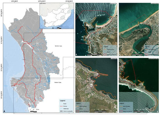
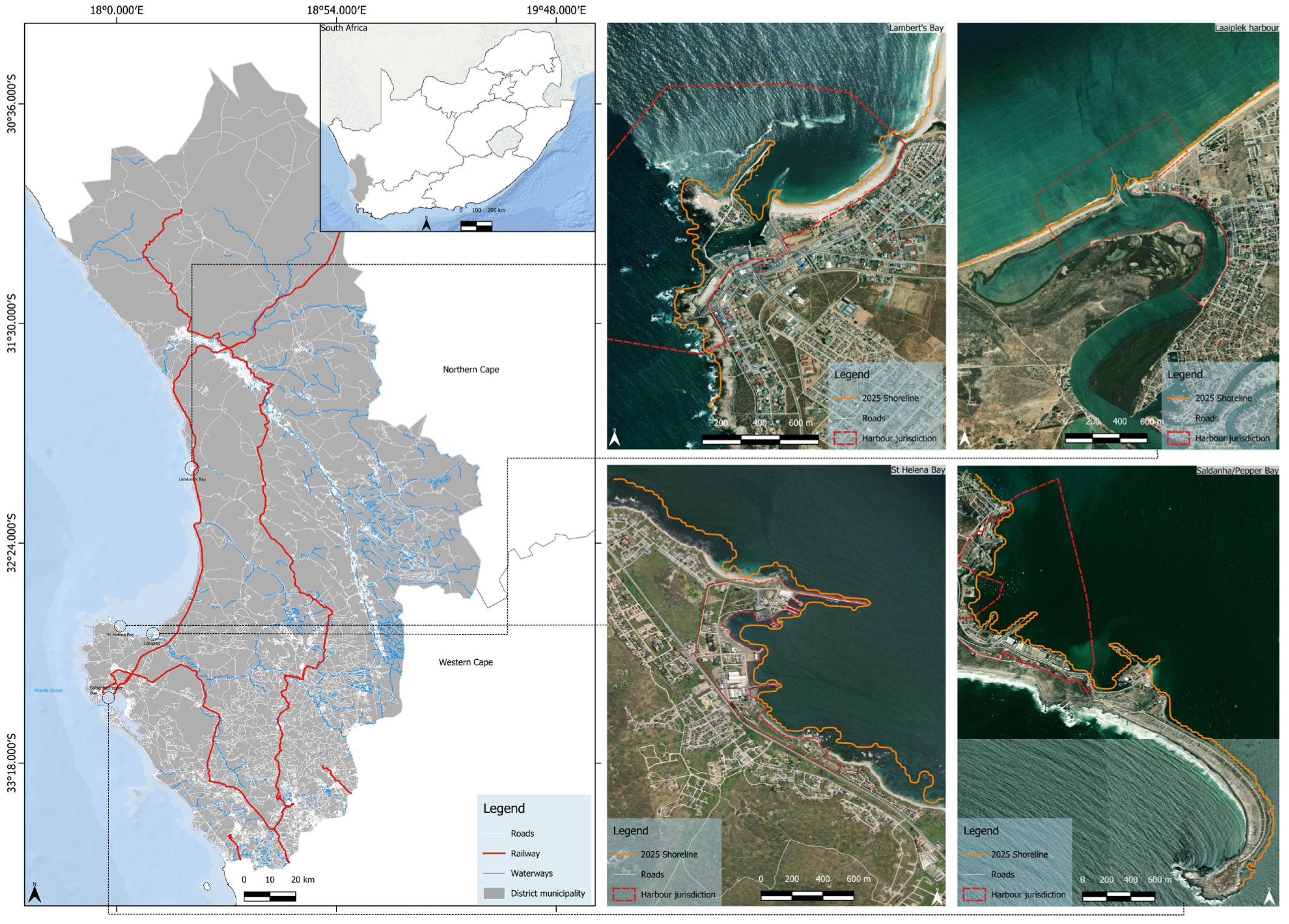
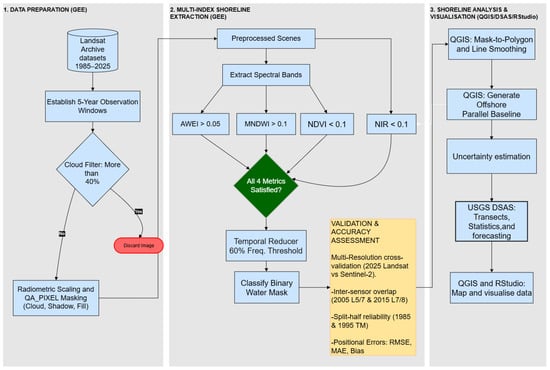
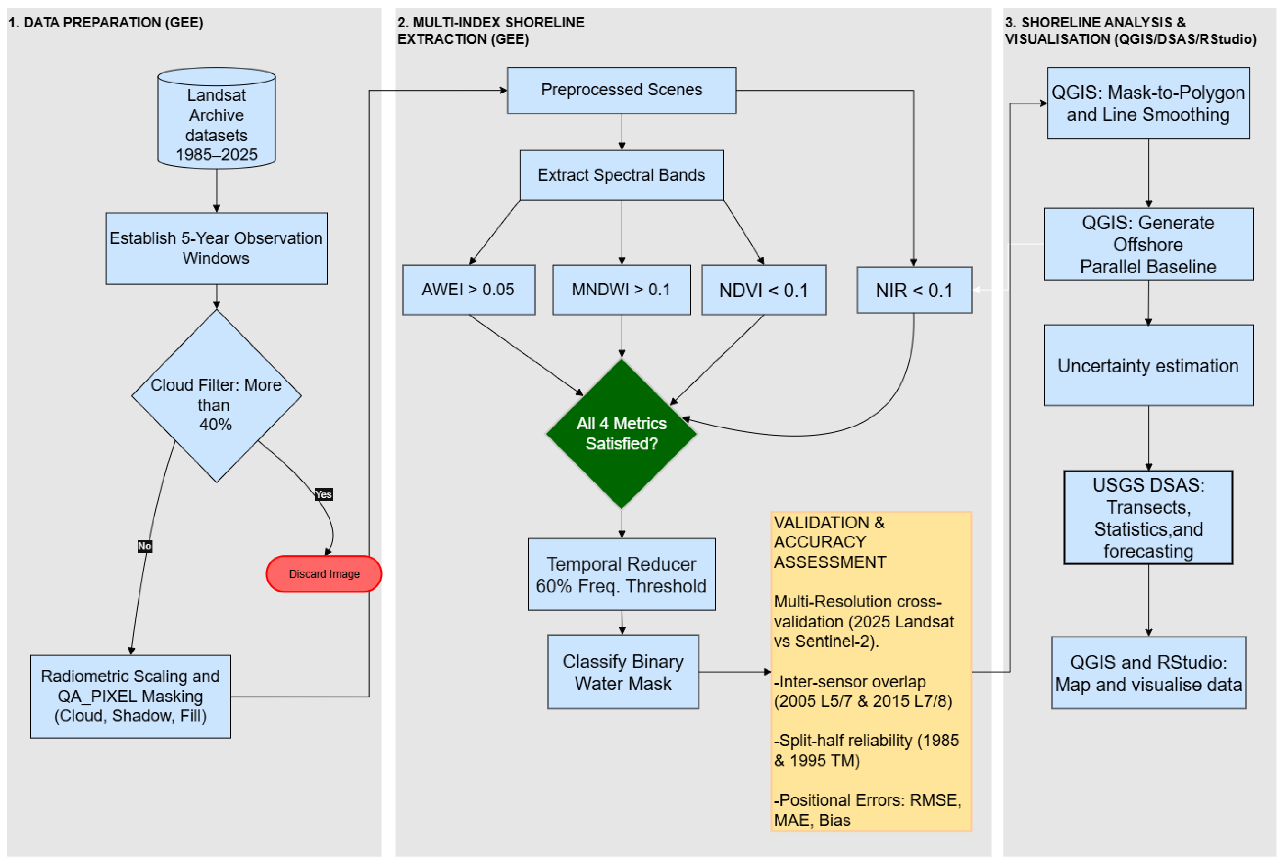
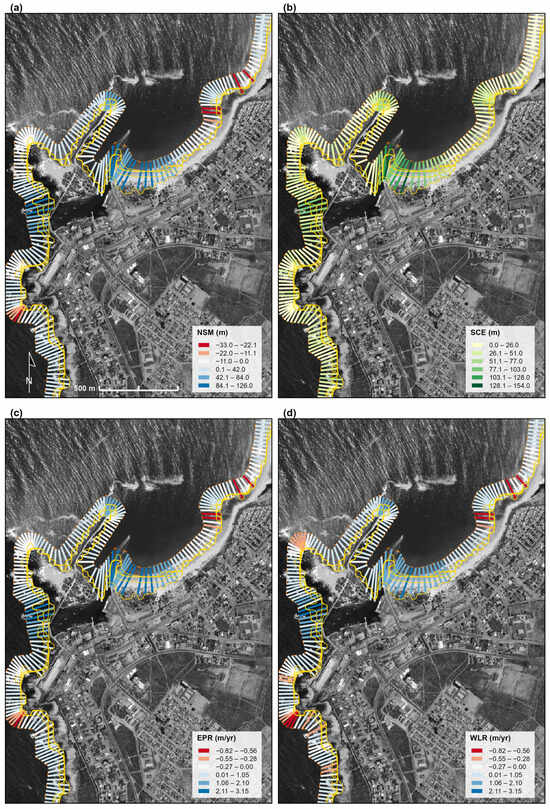
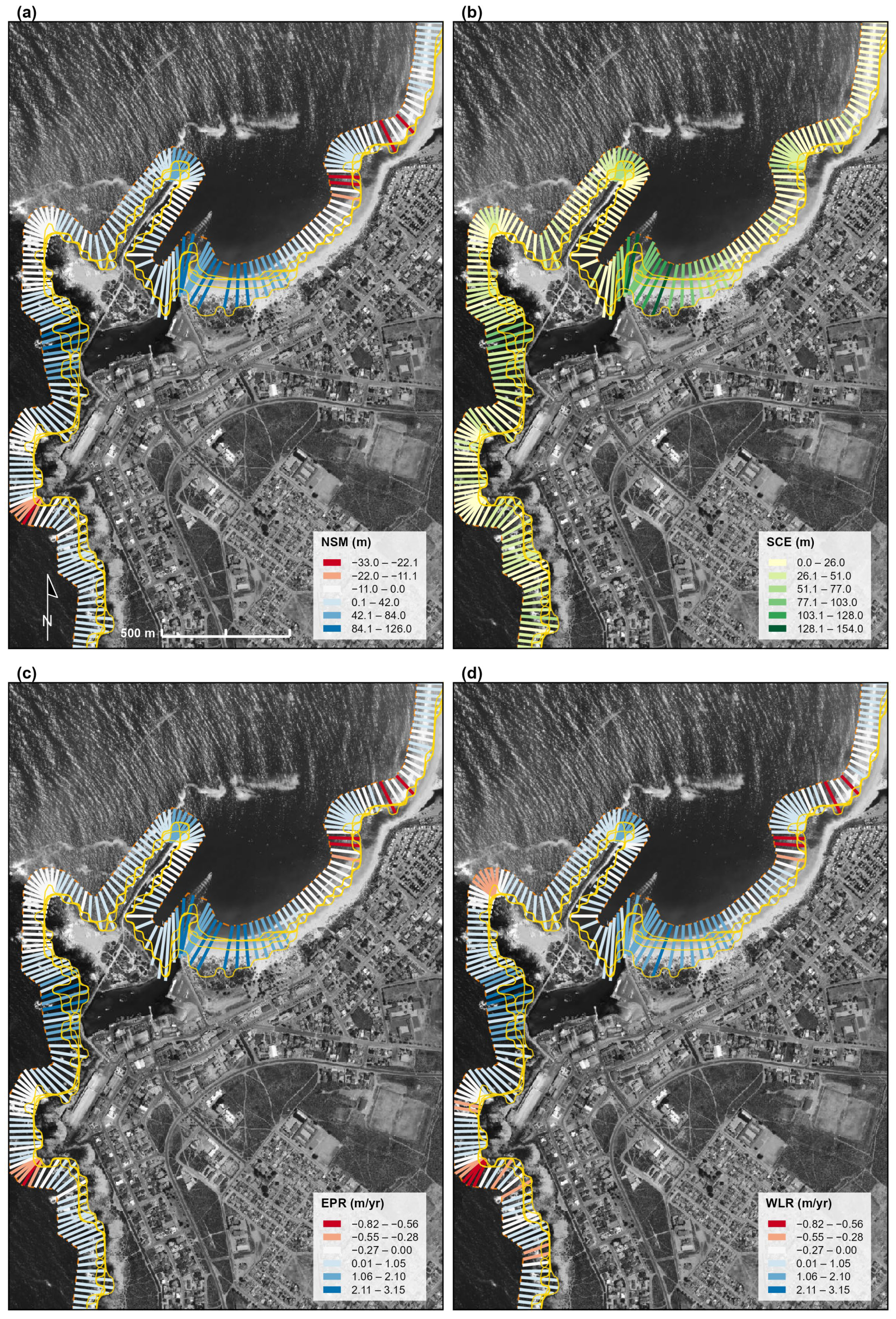
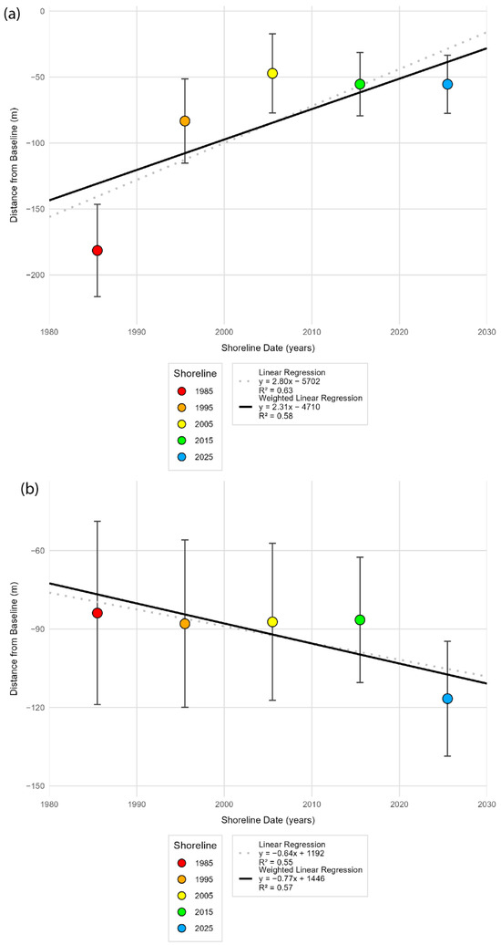
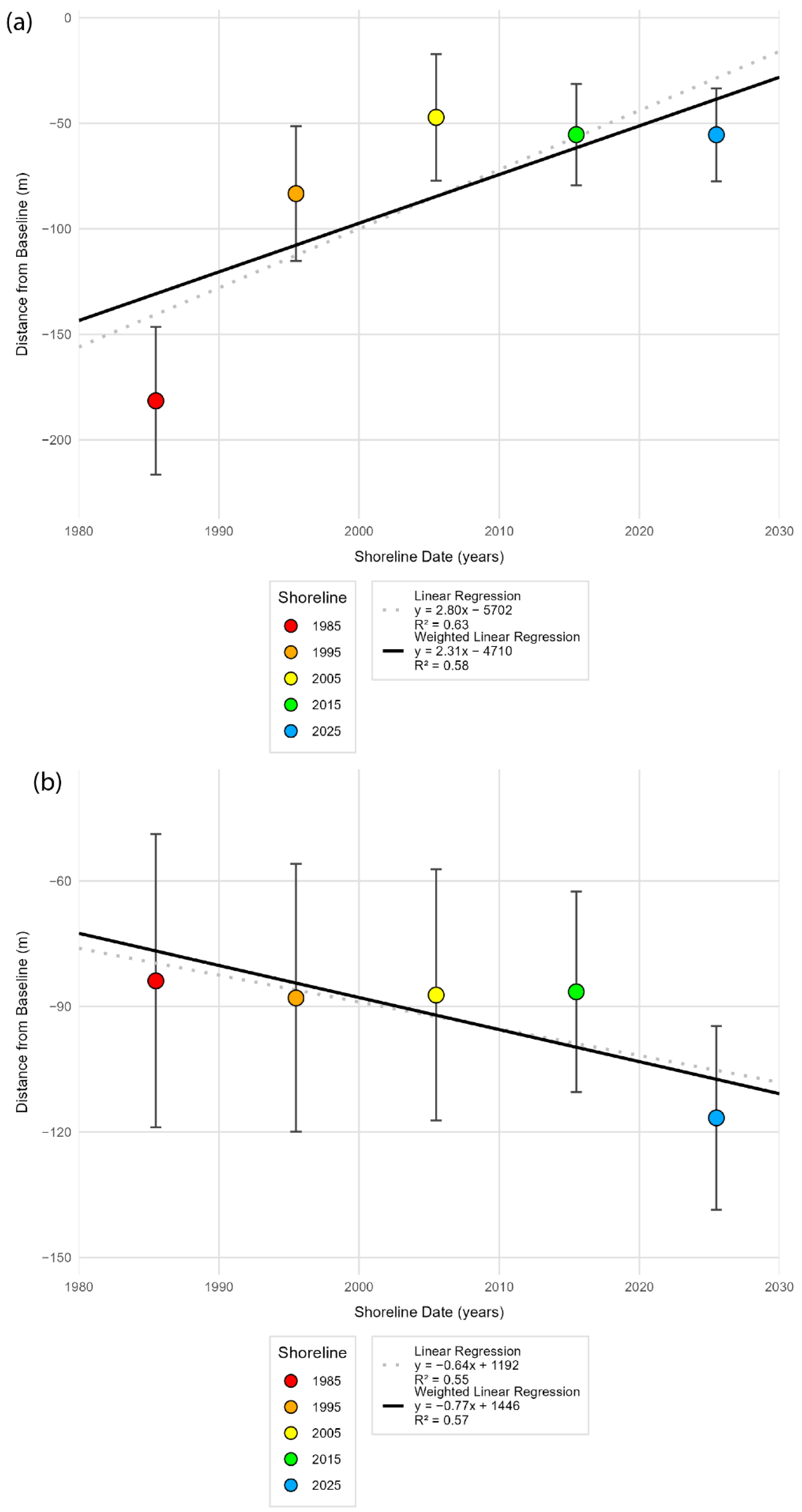
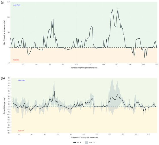
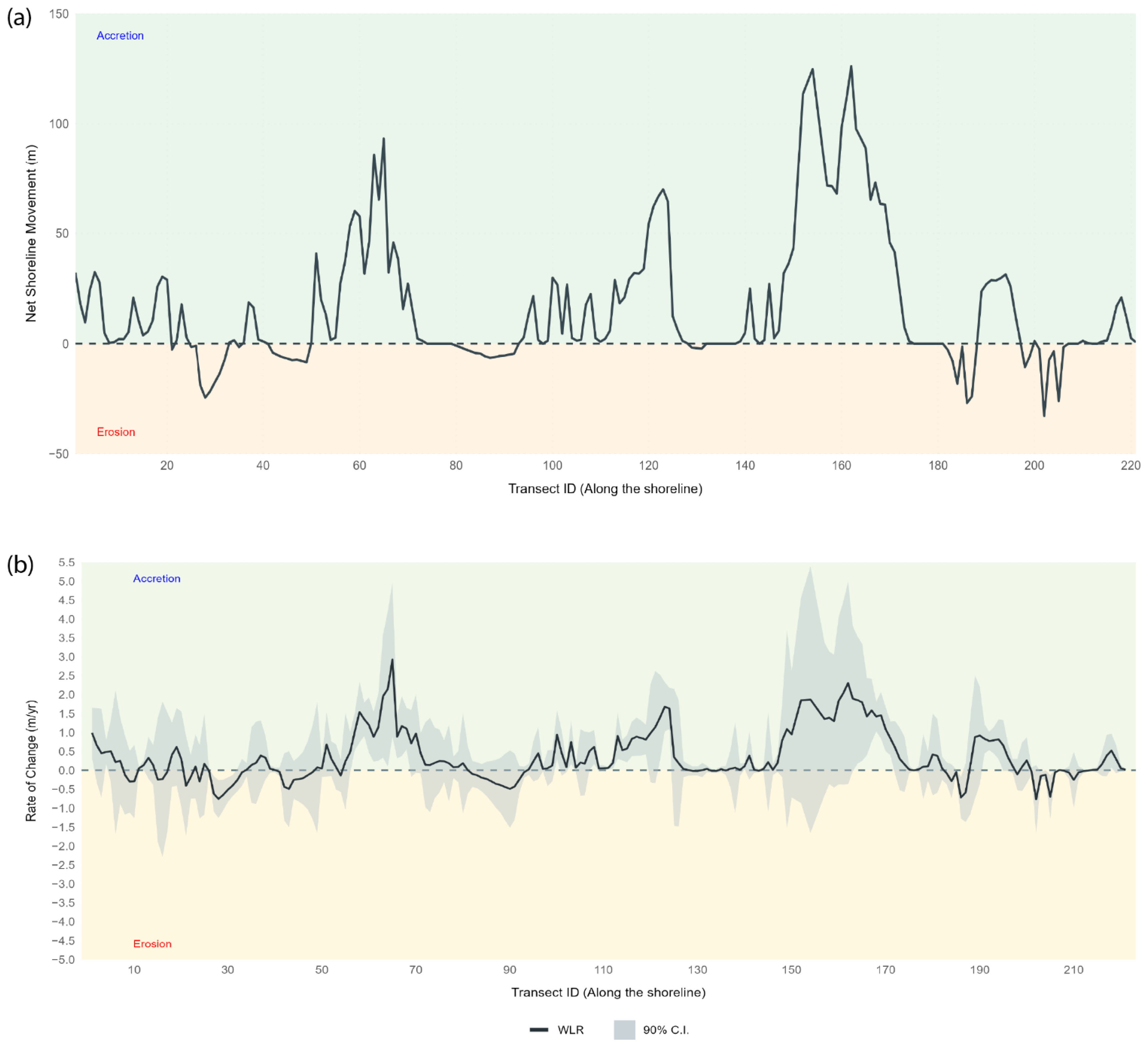
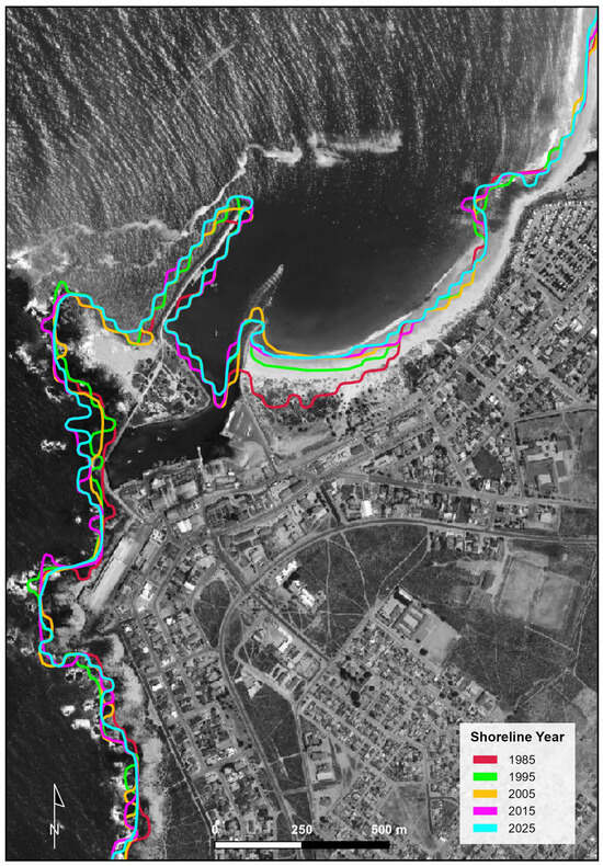
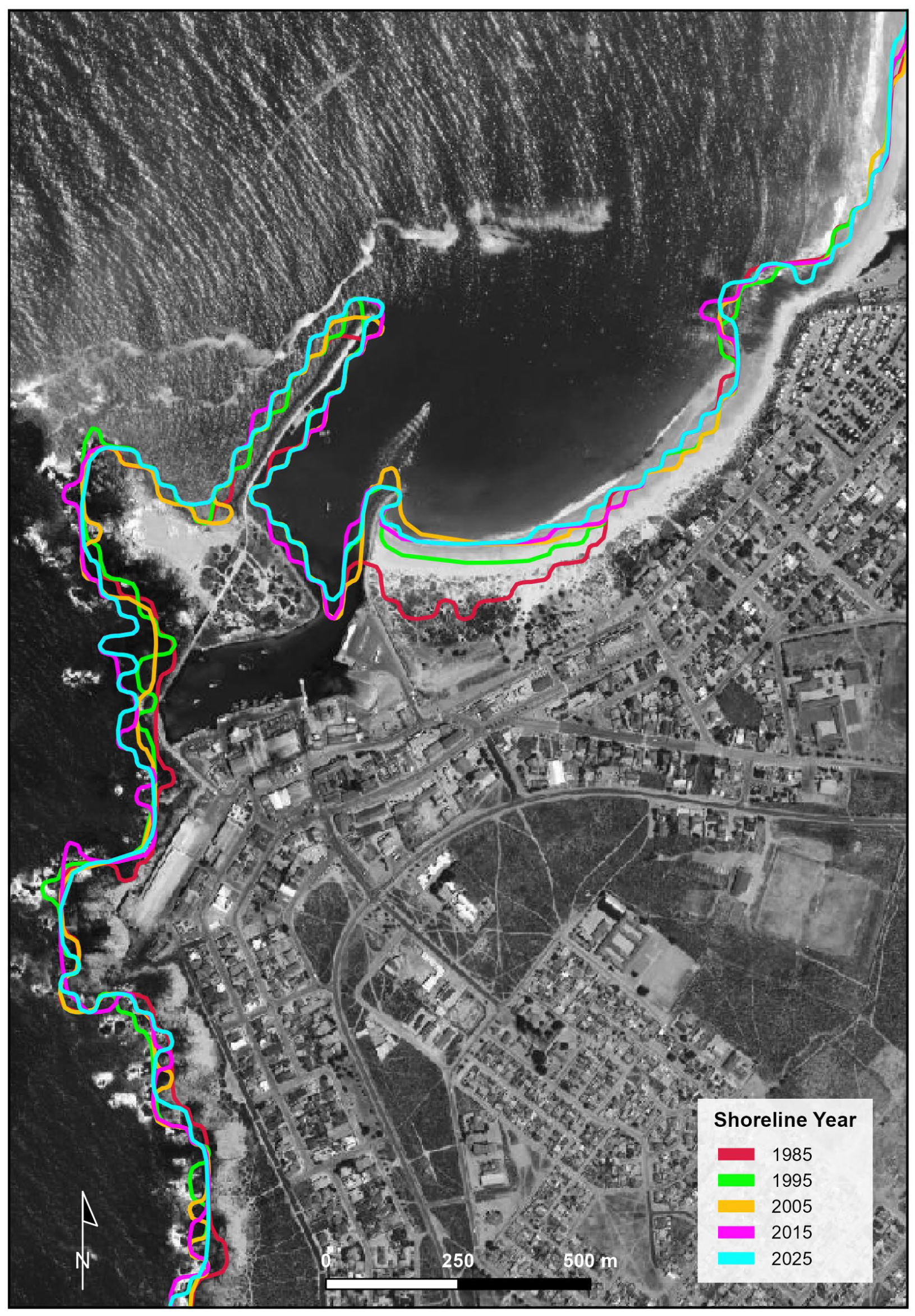
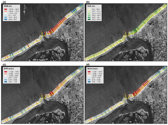
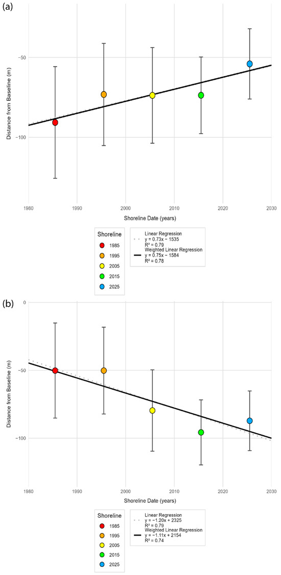
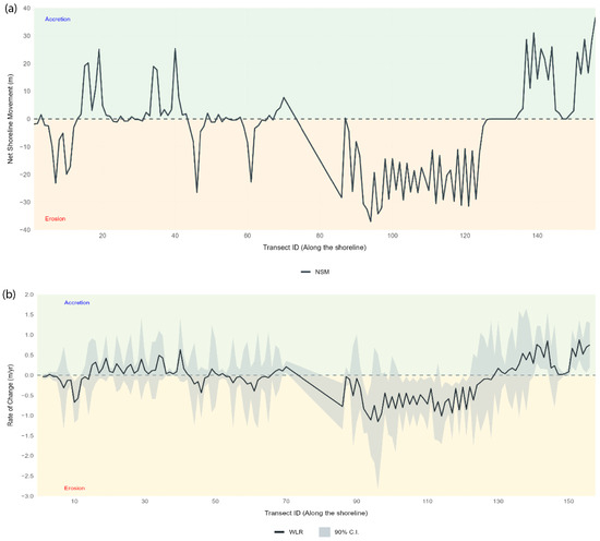
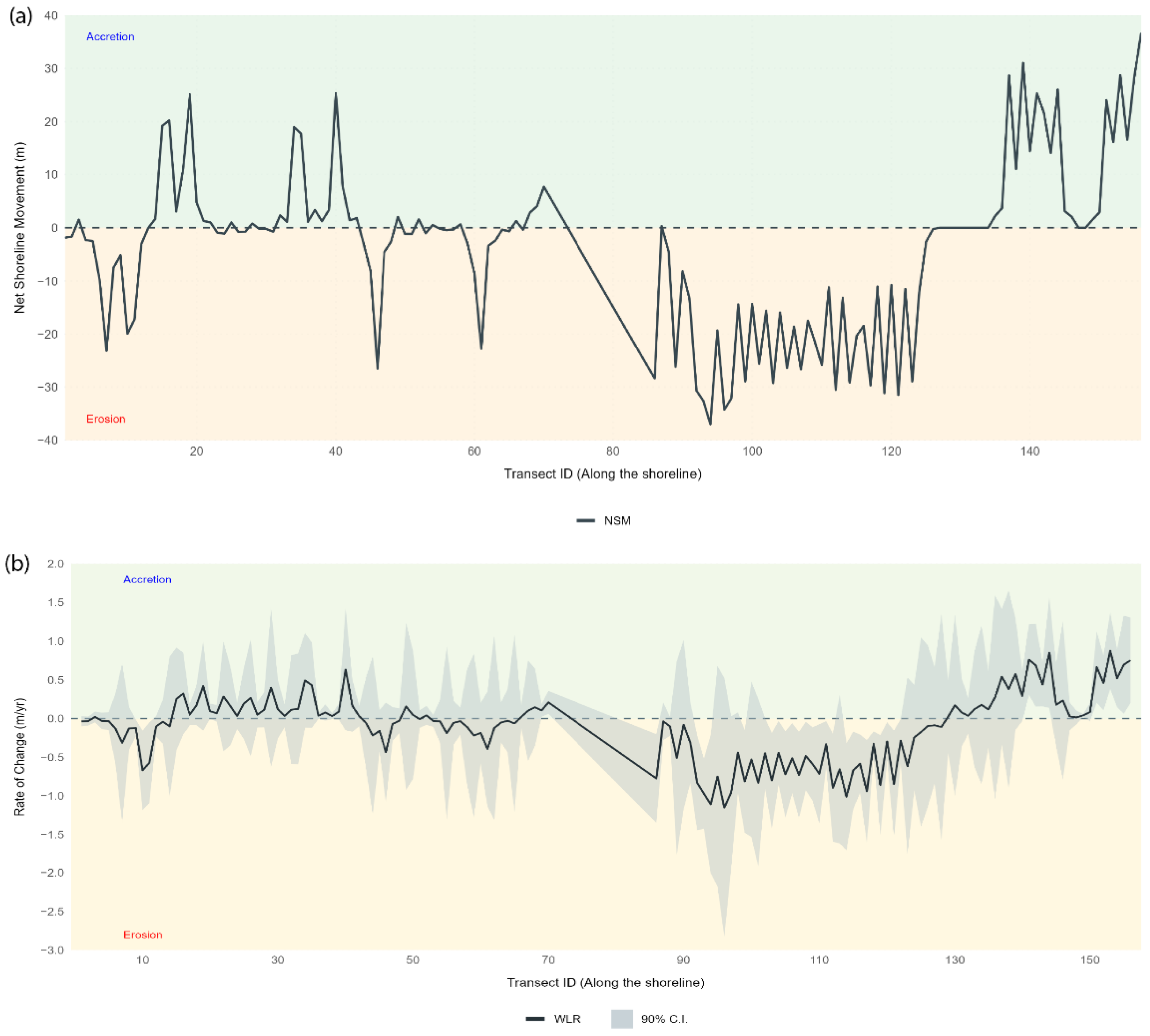
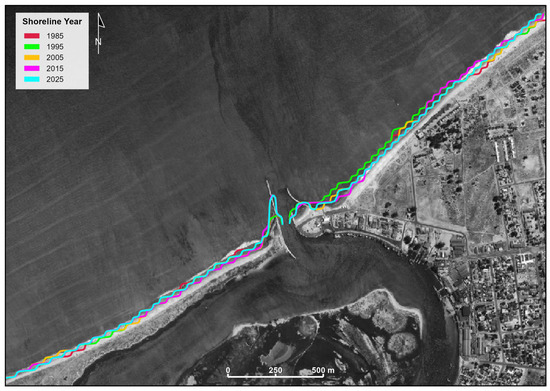
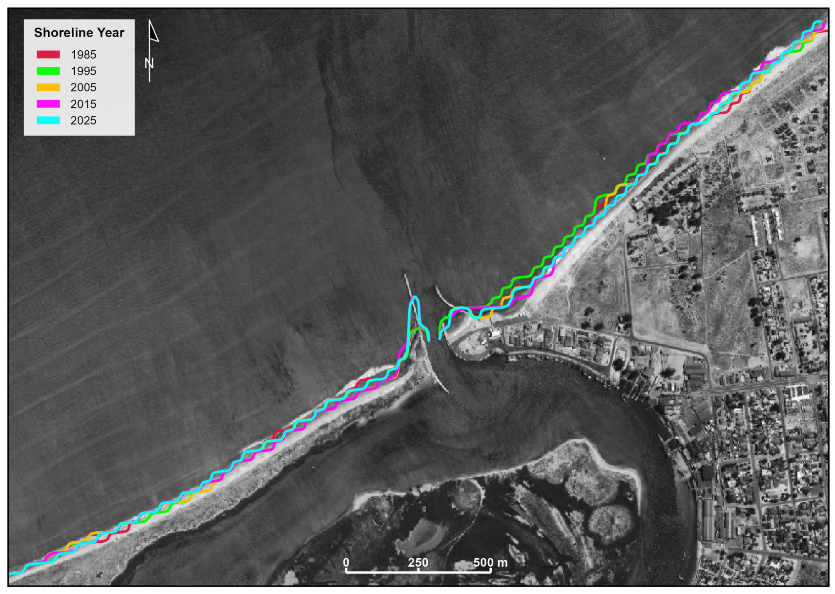
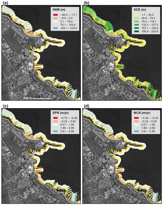
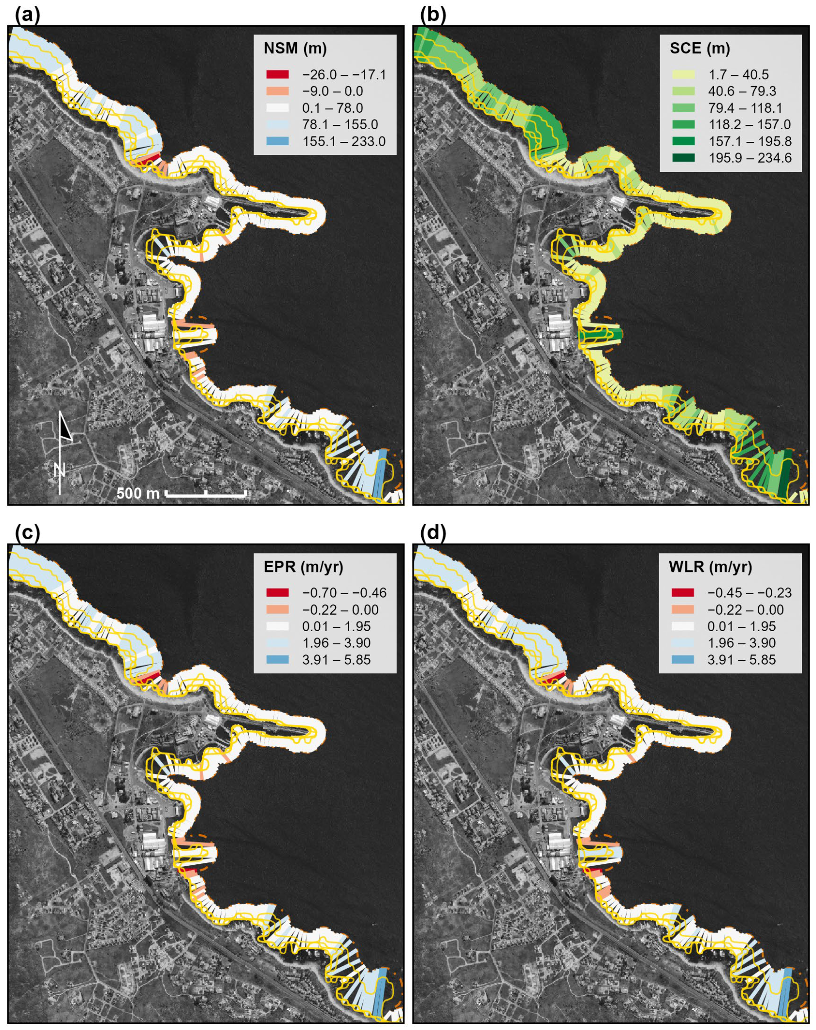
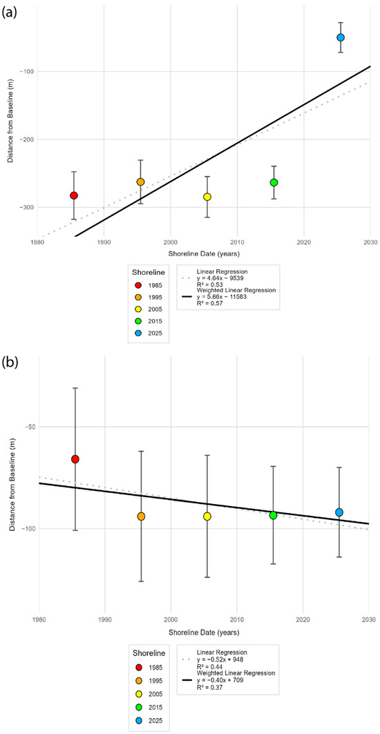
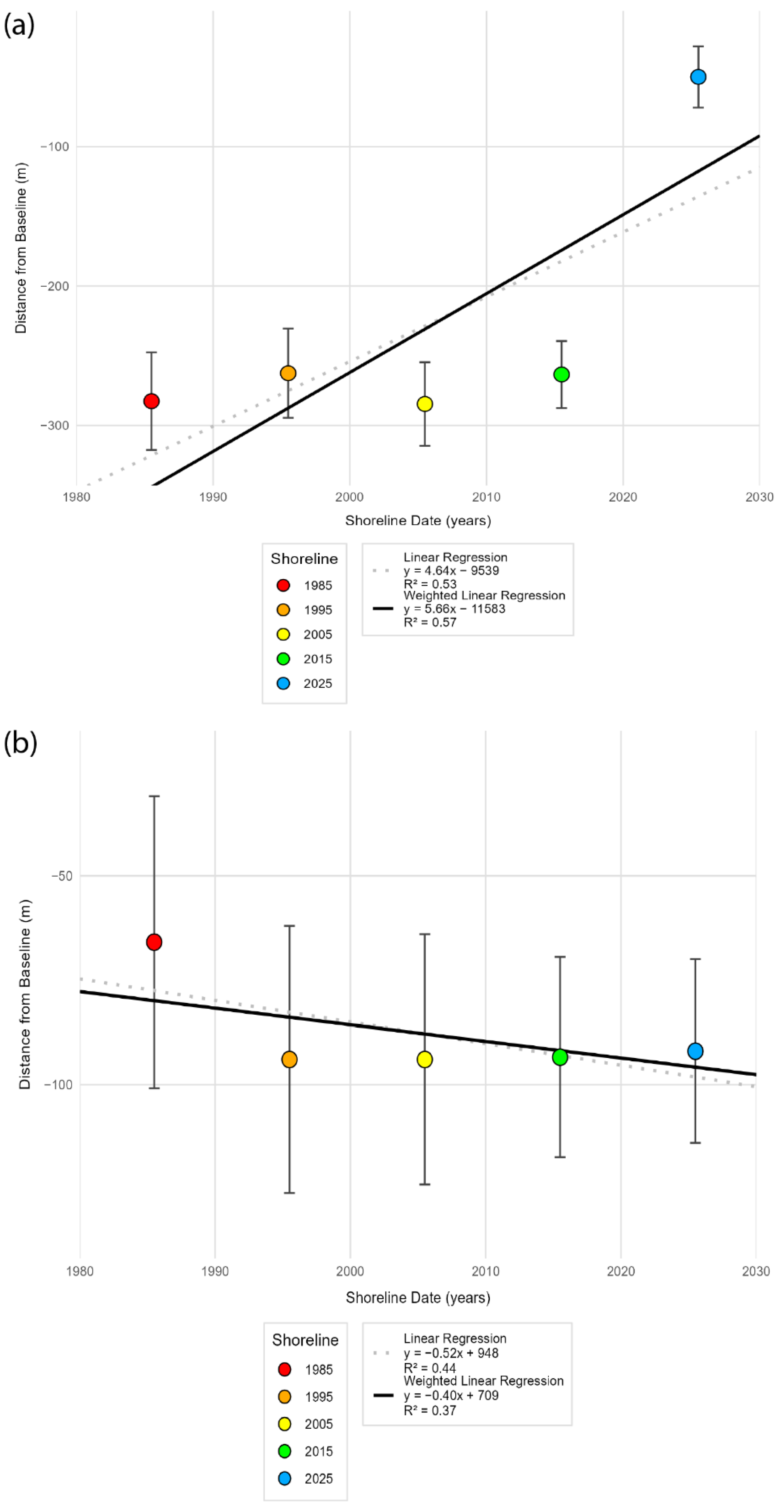
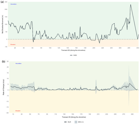
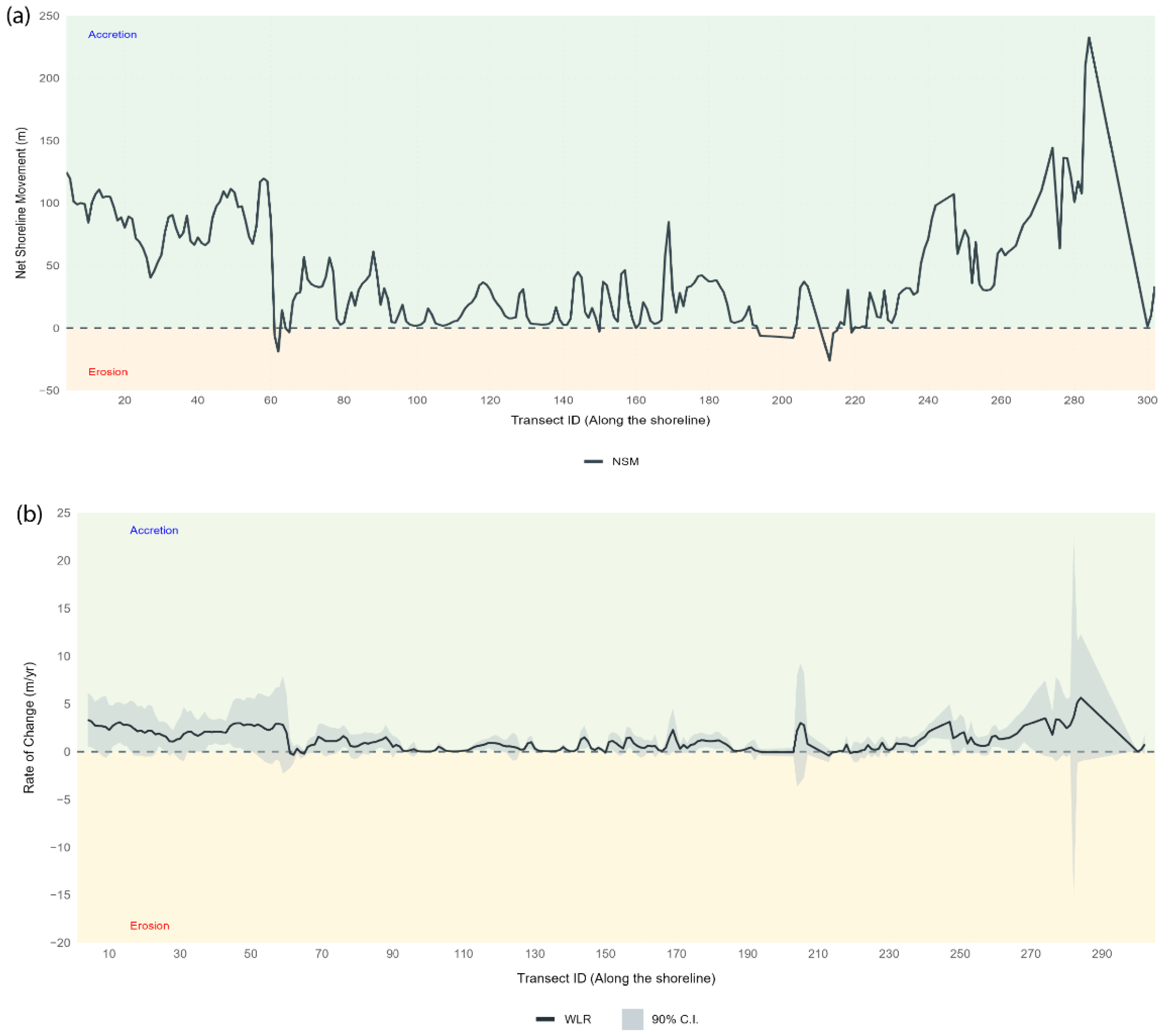
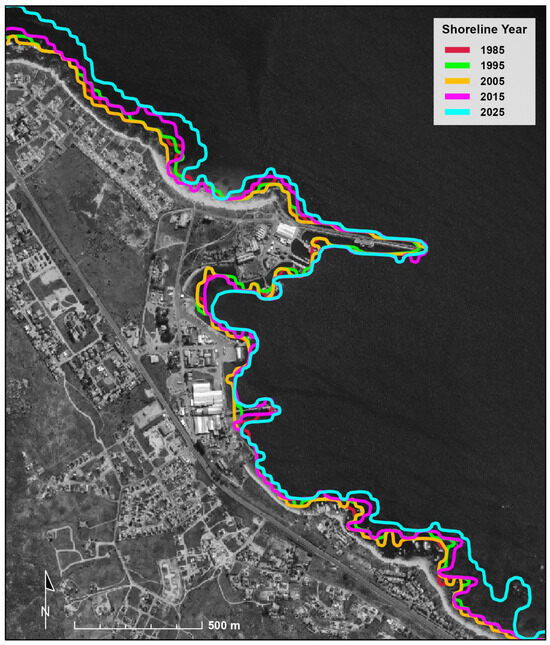
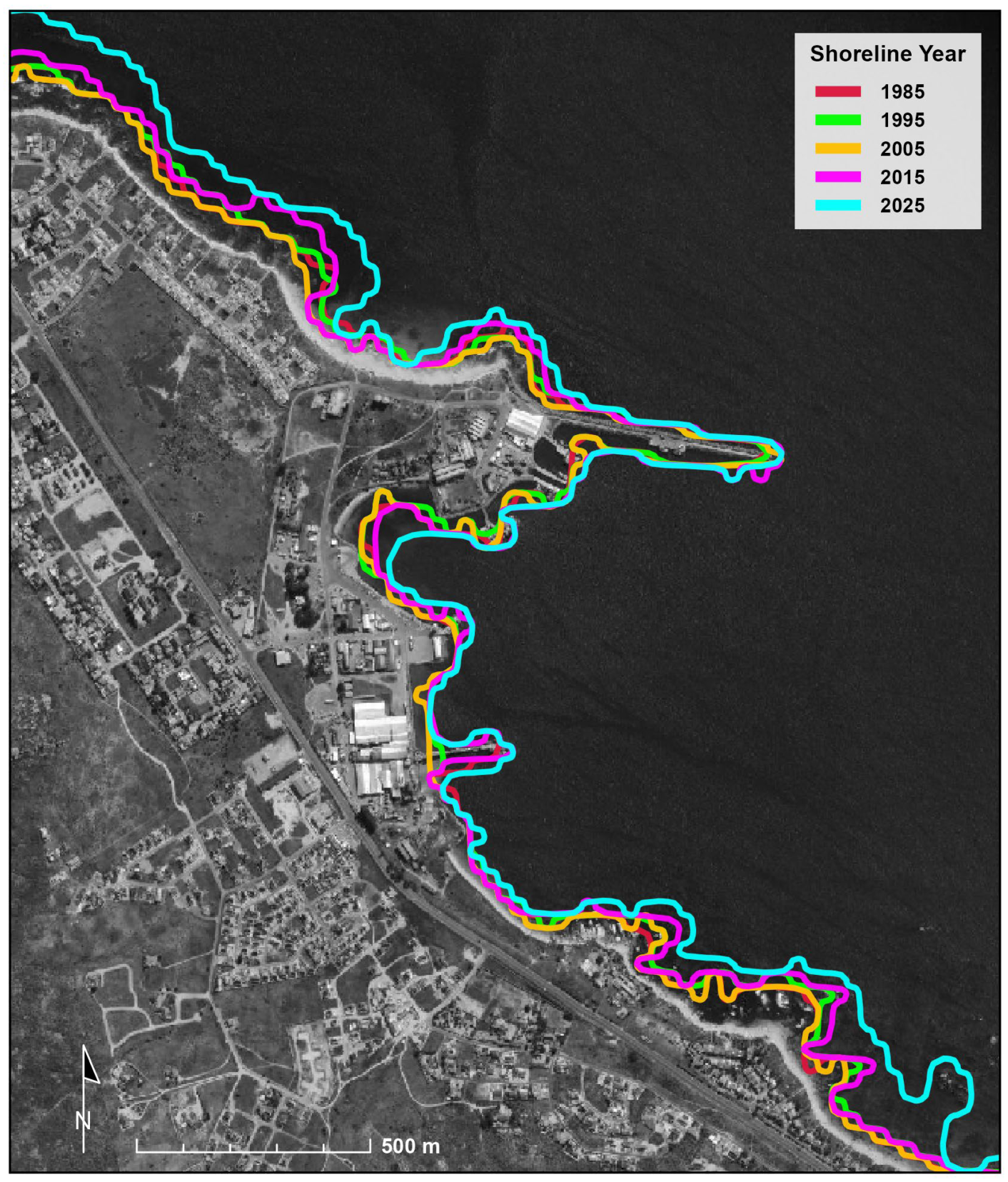
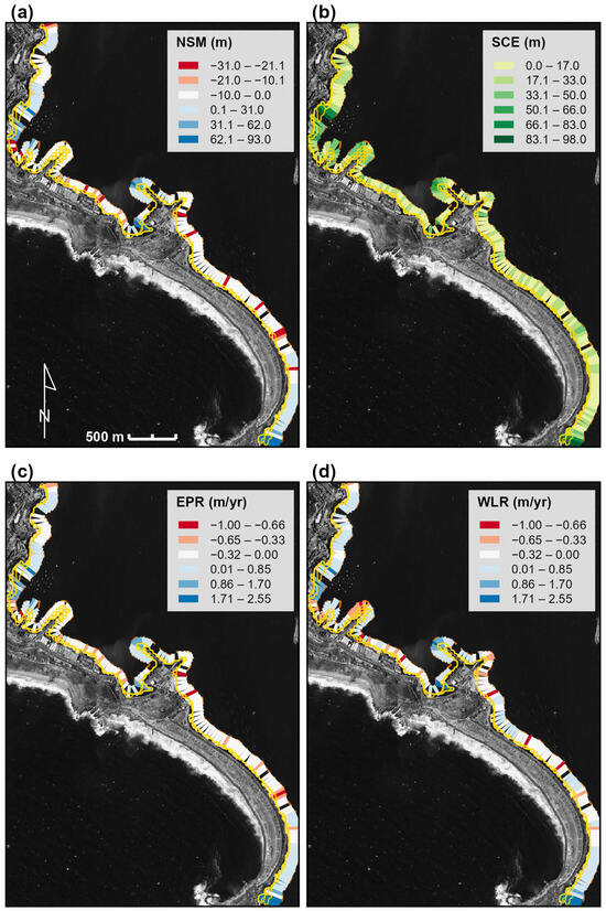
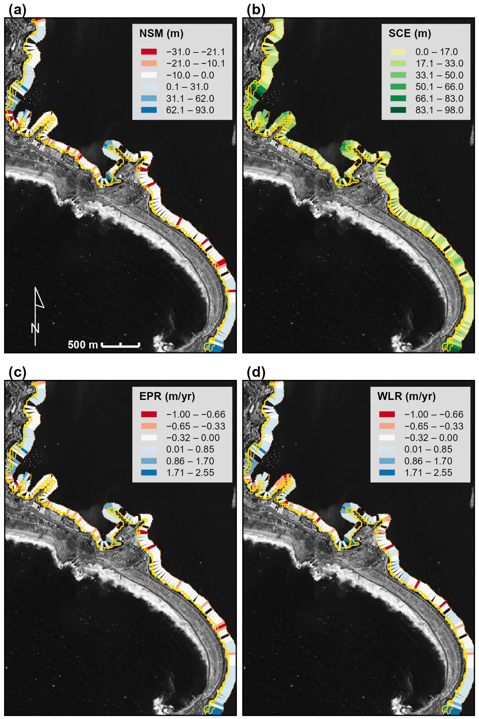
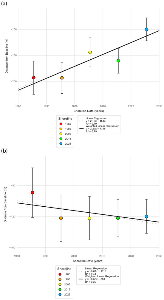
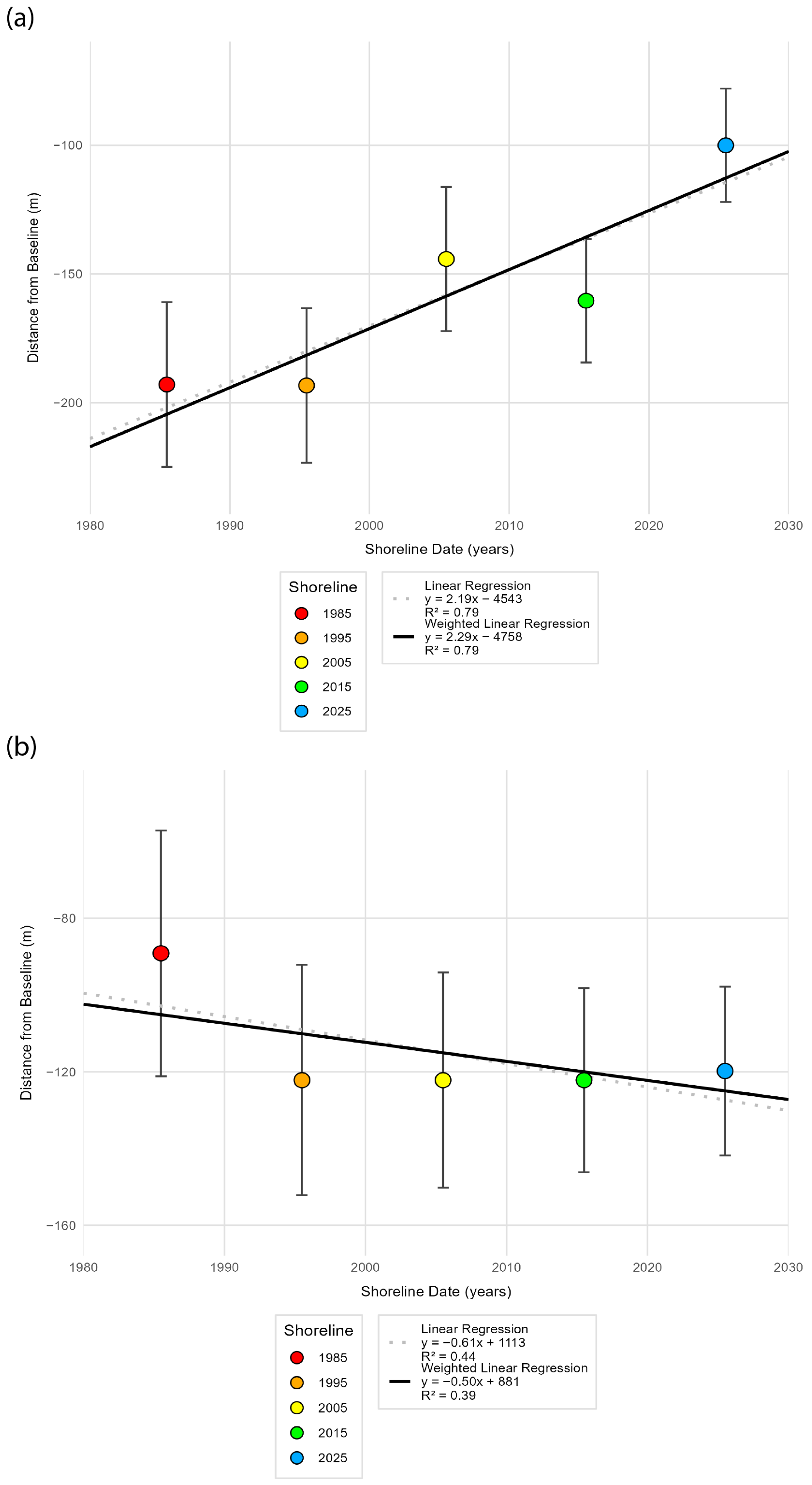
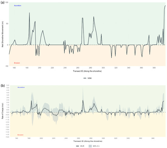
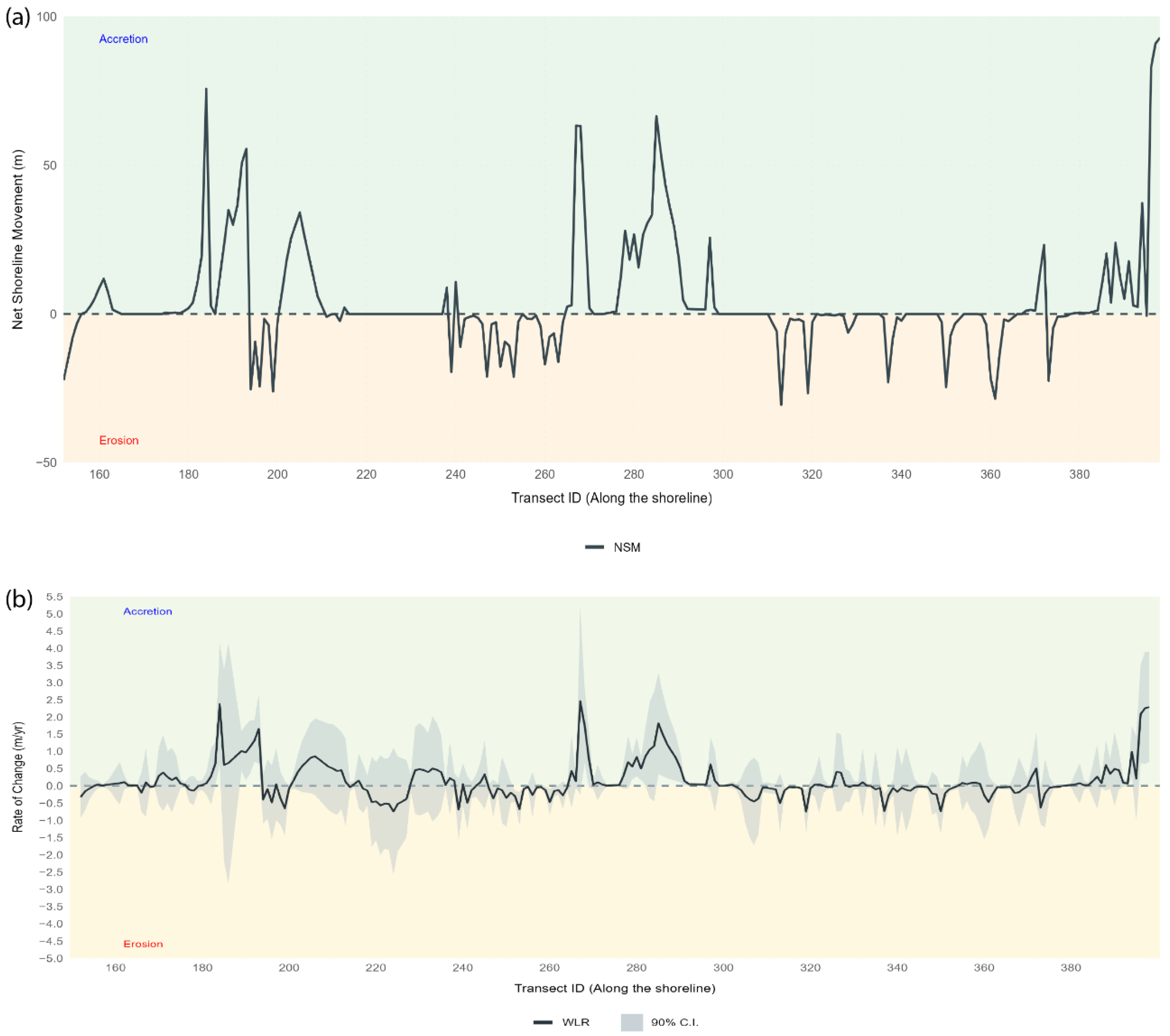
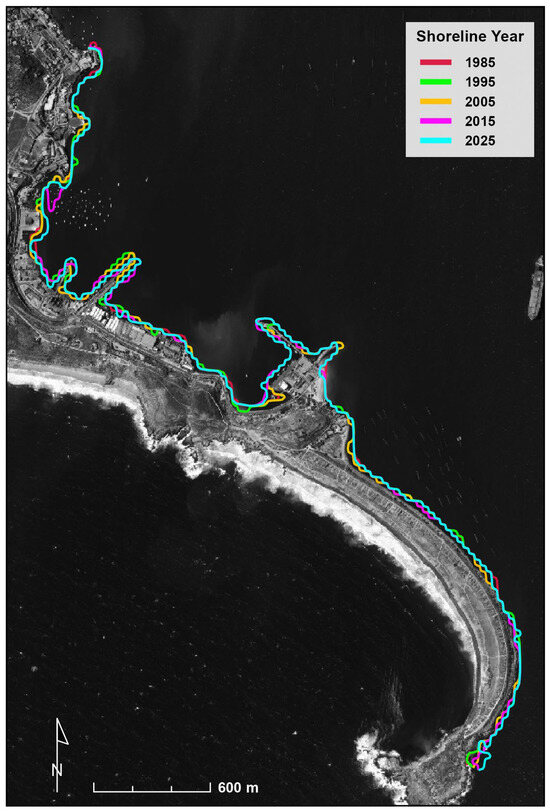
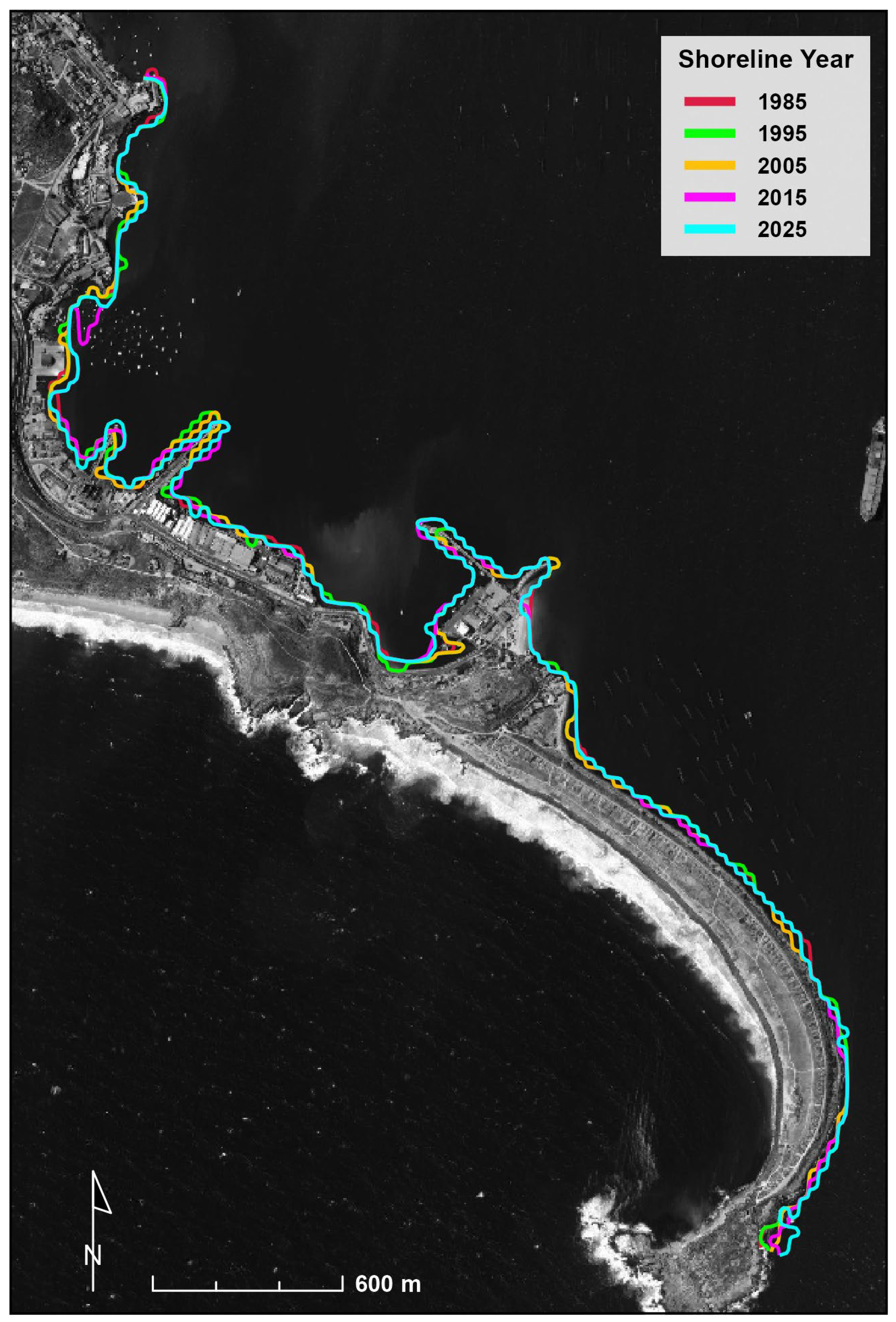
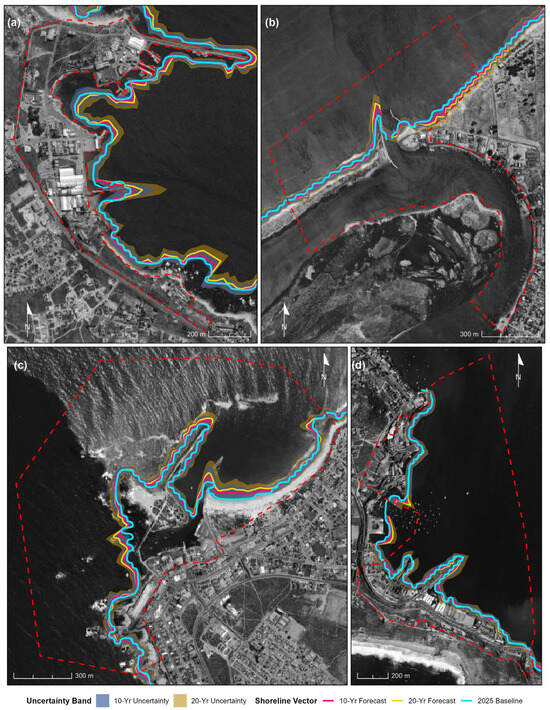
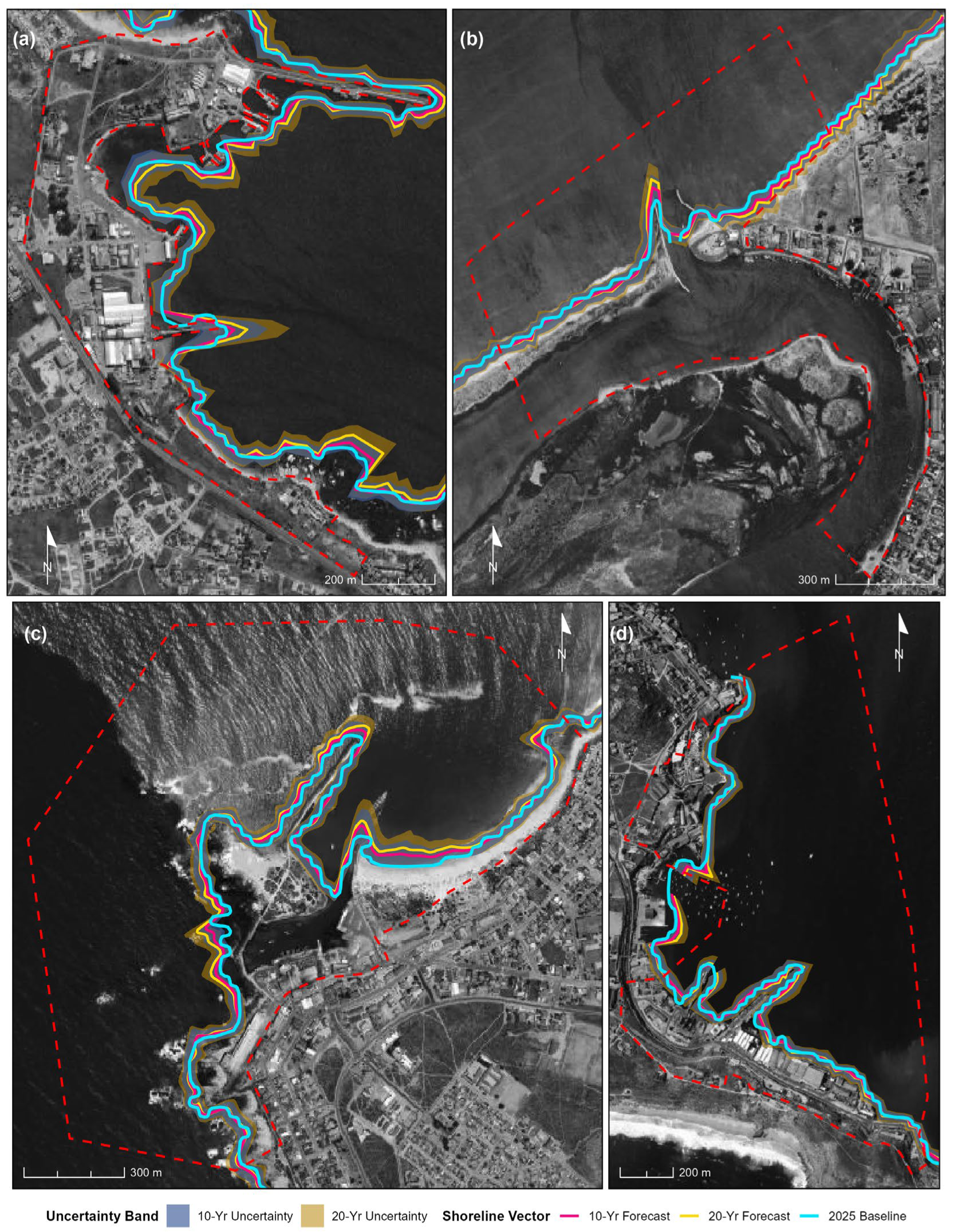

Disclaimer/Publisher’s Note: The statements, opinions and data contained in all publications are solely those of the individual author(s) and contributor(s) and not of MDPI and/or the editor(s). MDPI and/or the editor(s) disclaim responsibility for any injury to people or property resulting from any ideas, methods, instructions or products referred to in the content. |
© 2026 by the authors. Licensee MDPI, Basel, Switzerland. This article is an open access article distributed under the terms and conditions of the Creative Commons Attribution (CC BY) license.