


Abstract
This study considers temperature gradients over recent decades near Trujillo, Peru, (8.15 S, 78.95 W) using high-resolution data assimilation. Statistical analyses describe a steep gradient from the cool foggy coast to the warm coastal plains below the Andes. A cross-coast transect is analyzed for seasonal changes in maximum air temperature from SENAMHI station data interpolated with satellite infrared measurements. Weather forecasts aimed at the urban area show a cool bias at higher temperatures and often under-represent the landward increase of 5 °C/10 km, induced by wind-driven upwelling and turbulent heat flux. Morning fog-stratus tends to delay diurnal heating on the beachfront, whereas, a few kilometers inland, warming occurs due to the segregating effect of channeled long-shore winds. Although seasonality is limited near Trujillo, winter exhibits the greatest variance of maximum temperature due to fluctuations of cloud albedo. Regressions of temperature time series onto meteorological fields identify that a subtropical trough/ridge pattern leads to higher winter values due to weaker upwelling, warmer sea temperatures, and reduced fog-stratus. Long-term trends for increased sea/land gradients have implications for the adaptation to climate change.
1. Introduction
Peru is located at tropical latitudes with steep mountains and cold currents. The coastal weather is dominated by shallow equatorward winds and oceanic upwelling [1]. Evaporation is suppressed, but condensation is enhanced, leading to fog and stratus. A downward heat flux causes atmospheric subsidence and thermal stability. The seasonal cycle is of low amplitude, giving cities such as Trujillo (at 8.15 S) an ‘Eternal Spring’. The semi-arid coastal plains are intersected by river valleys that conduct runoff from the 4000 m Andes Mountains located <100 km inland [2]. More than half of the population of Peru live near the shore, exposed to strong air temperature gradients.
Daily weather forecasts have been evaluated for the coast near Lima (12 S) by comparison of short lead-time outputs from numerical and statistical models, that take account of meteorological evolution [3]. Human interventions are needed to translate the model data for a variety of applications. The key weather systems altering temperatures have been identified. During summer, moisture advection between the Bolivian High and the tropical troughs (amplified by El Niño) is the most influential [4,5,6,7]. During winter, mid-latitude westerly waves affect the coastal weather via cold surges that strengthen the marine anticyclone’s southeast winds and currents [8,9,10]. A comprehensive study [3] found that daily temperature changes related to low-level winds and cloudiness and that model skill was poor during winter (June–August).
Here, the role of air–land–sea interactions and surface heat fluxes in local temperature gradients is quantified. Cool SSTs underlie shallow equatorward winds, producing gray skies on most winter mornings. During the afternoon, air temperatures often increase rapidly inland and contribute to forecast ‘errors’. An analysis is made of the annual cycle of cross-shore air temperature gradients near Trujillo, Peru, whose one million inhabitants sprawl ~8 km inland. A variety of datasets are employed to illustrate the processes affecting this gradient. The aim is to characterize the drivers and impacts of coastal air temperature gradients, to improve operational forecasts and the adaptation to climate change impacts.
2. Data and Methods
The coastal meso-climate of Peru is analyzed on an hourly to monthly timescale using satellite, reanalysis, and in situ datasets over the period 2001–2024. Peru’s national weather service SENAMHI collects local observations from a network of weather stations, radiosonde and aircraft profiles, and frequent ship surveys, supported by global remote sensing and coupled data assimilation. Ref. [11] describe sophisticated methods to interpolate these data into high-resolution fields for Peru, making use of Modis satellite observations since 2001. These data are employed in high-resolution cross-shore transects.
Seasonal climatologies were calculated from Modis satellite land surface daytime temperatures and vegetation color fraction at a 1 km resolution over the study area 8.8–7.4 S, 79.6–78.4 W. The diurnal cycle of sensible heat flux is calculated from hourly CFS2 reanalysis at the Trujillo grid-point (8.15 S, 79.0 W). Seasonal wind frequency distributions were constructed from hourly observations at Trujillo airport. Satellite sea surface temperatures were statistically analyzed both locally and over a wider area, 25 S–8 N, 95–68 W, for the long-term mean, seasonal averages, and standard deviation. Climate change was addressed by the calculation of linear trends in the period 1980–2024 for SST, air temperature, and the meridional Hadley circulation averaged for coastal longitudes.
A transect was analyzed along 8.15 S, 80–78 W for ERA5 maximum air temperature, sensible heat flux, and satellite cloud albedo, to identify cross-shore gradients and was downscaled to achieve a 2 km resolution. ERA5 daily maximum and dewpoint temperature records were extracted at the Trujillo grid-point (N = 8765) and analyzed for lag auto-correlation, wavelet spectral amplitude, and mean annual cycle in the period 2001–2024. Validations were performed by comparing model-assimilated air temperatures from ERA5, CPC, GFS, and CFS2 with Trujillo airport observations and calculating the Pearson’s product-moment linear coefficient over the 8765 days.
The Trujillo daily maximum temperature time series 2001–2024 was high-pass filtered above 60 days to remove seasonal variability, then regressed onto June–August fields of sea-level air pressure, 500 hPa geopotential height, sea surface temperature, satellite net OLR, and surface wind velocity to determine the spatial patterns driving the winter weather, as in [3]. These regressions provide over 4000 realizations to evaluate field significance.
Seasonal climatologies were calculated along the 8.15 S transect from SENAMHI (PISCOt v1.3) maximum air temperature averages and root mean square anomalies (variance) to identify micro-climatic gradients around Trujillo. Hovmoller plots were made along the transect to reveal intra-seasonal pulsing of land surface temperature, sea surface temperature, and potential air temperature. Cases were identified from these analyses, to study a late winter cool spell (1–2 September 2020) via 500 hPa wind maps, hourly CFS2 wind and temperature near Trujillo, sea temperatures, and near-surface airflow back-trajectories from Hysplit.
On 6 and 12 July 2025, a condition of dense winter fog-stratus was analyzed via radiosonde profiles, hourly in situ weather observations, satellite visible imagery, and atmospheric circulation data. The mean annual cycle of offshore and inland cloud albedo was calculated and compared with the quintile range of the maximum temperatures. A satellite lidar aerosol height-section in dense fog-stratus was analyzed for 13 July 2008 and comparative cross-sections of long-shore wind and ocean upwelling were studied. Dataset acronyms and details are listed in Table 1.
Table 1.
Dataset characteristics.
3. Results
3.1. Seasonal Climatology
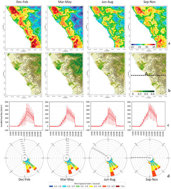
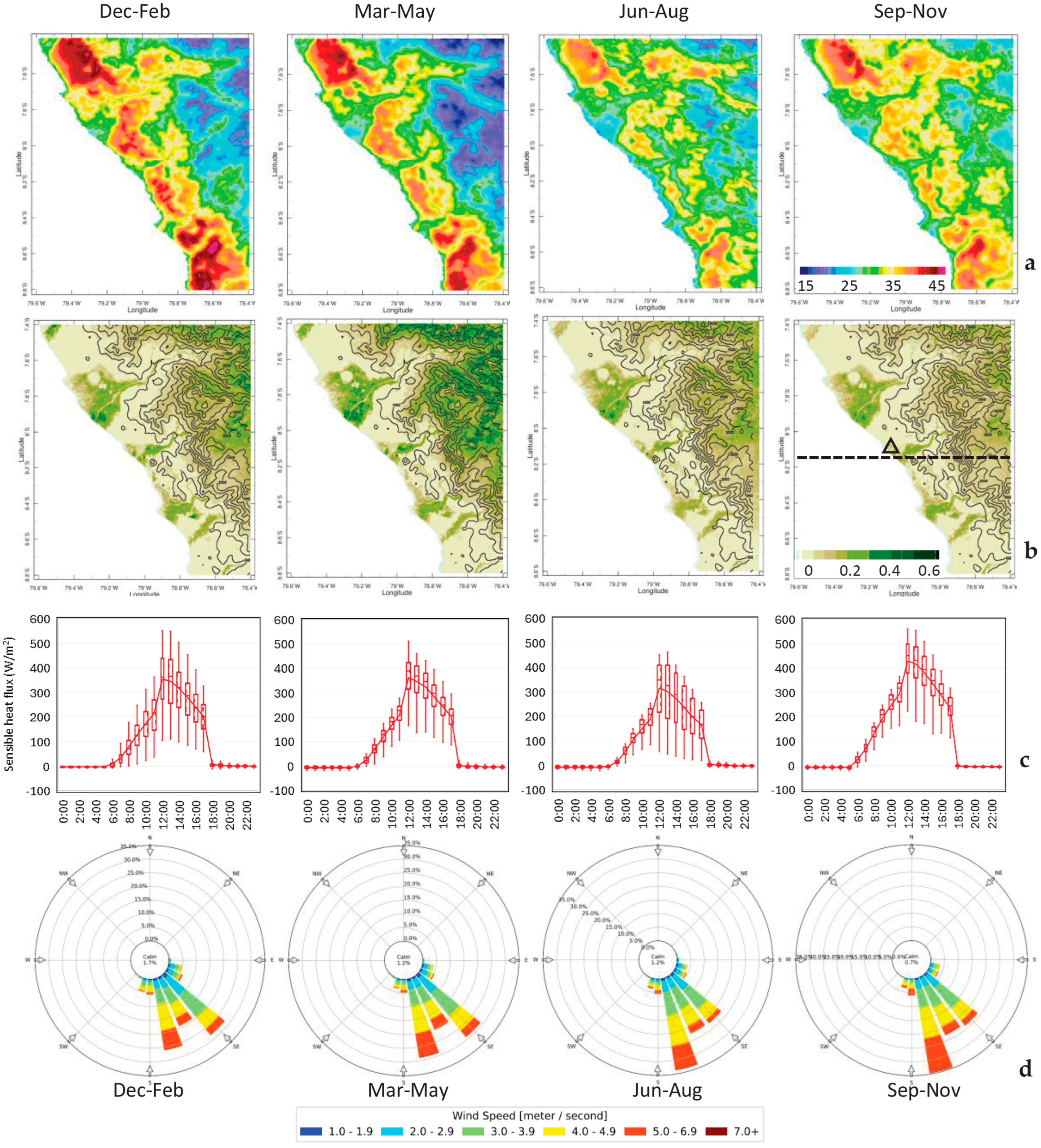
The 2001–2024 seasonally averaged 1 km resolution Modis satellite land surface daytime temperatures and vegetation fraction maps are presented in (Figure 1a,b). The temperatures show three zones around the Trujillo area: cool beachfront (19 °C), warm coastal plains (24 °C), and cold mountains (12 °C). The seasonal changes in temperature are minor, but higher temperatures across the coastal plains are moderated by vegetated river valleys. Coastal vegetation remains steady, while interior mountains exhibit seasonality. The mean diurnal cycle of sensible heat flux at Trujillo (Figure 1c) exhibits an asymmetric crest of 350–400 W/m2. The greatest variance occurs in winter at 12:00–14:00 h due to the variable depth, penetration, and timing of fog-stratus. Seasonal wind frequency distributions at Trujillo airport (Figure 1d) show a persistent SSE wind of 3.8 m/s with calm reported <2%. Few locations in the world have so little change in airflow from summer to winter.
Figure 1.
Seasonal (left to right: summer, autumn, winter, spring) mean maps of the following: (a) Satellite daytime land surface temperature. (b) Satellite vegetation color fraction with topographic contours, dashed transect, triangle station at right. (c) Seasonal box-and-whisker plots of the mean diurnal cycle of CFS2 sensible heat flux at Trujillo, 8.15 S, 78.95 W. (d) Mean wind roses at TRU airport (left to right) by season; outer ring is 35%, based on hourly observations over the period 2001–2024.
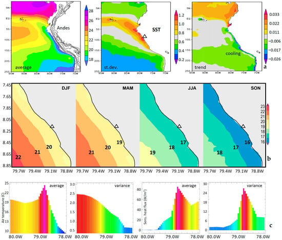
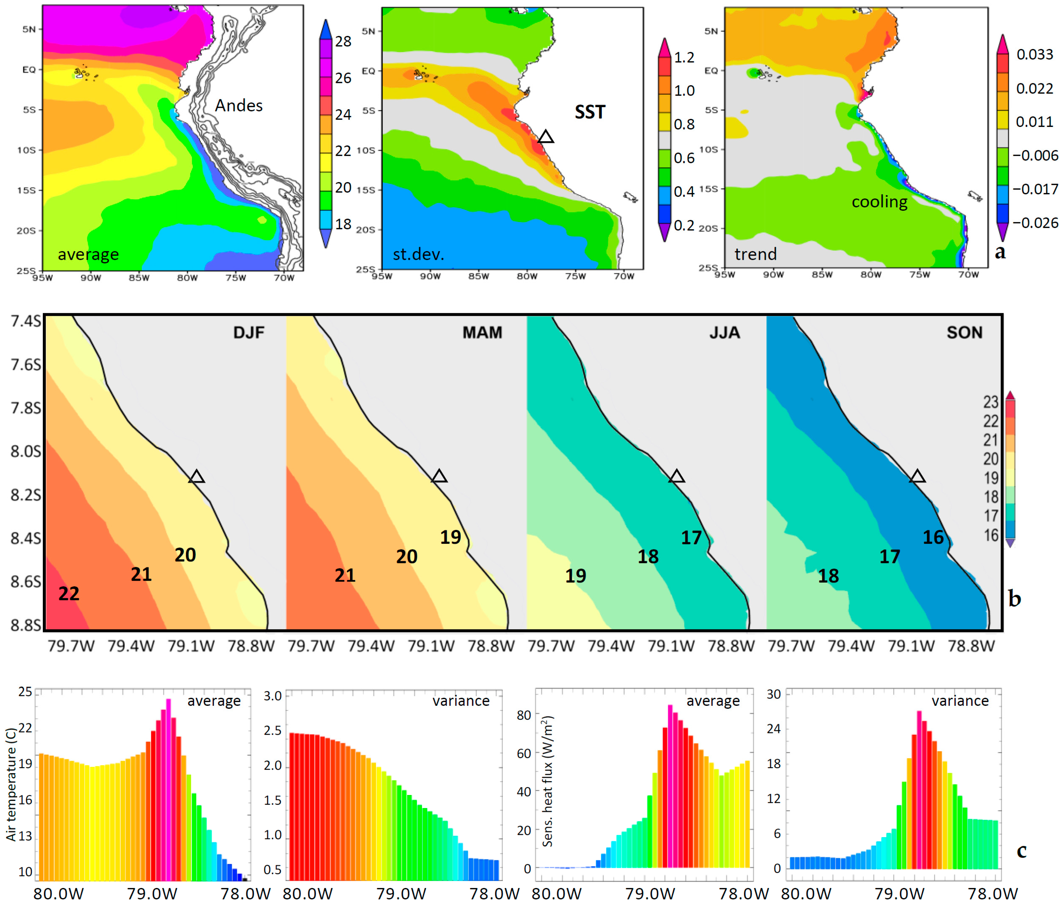
The regional sea surface temperatures (Figure 2a) exhibit a cool wedge that broadens southward. The maximum standard deviations extend from Trujillo to the Galapagos Islands, a ‘footprint’ of summer El Niño. The long-term trends (1980–2024) show cooling over the shelf of Peru, helping mitigate global warming, yet rapid warming over the interior [19] suggests steeper coastal air temperature gradients. The local SST patterns (Figure 2b) show minor differences across the seasons. Persistent wind-driven upwelling (16–20 °C) forms a cool inshore zone and a shallow atmospheric boundary layer (~300 m). Seen in a meteorological context, the airflow around the southeast Pacific anticyclone is channeled by the steep topography to produce a long fetch for condensation and persistent morning fog-stratus.
Figure 2.
(a) Regional SST (left to right) average, standard deviation, linear trend since 1980, topographic contours (left), triangle—Trujillo. (b) Local SST by season, averaged 2001–2024. (c) ERA5 air temperature and sensible heat flux (right) average and root mean square anomaly (variance) on the transect 8.15 S, with coast at 79 W, interpolated at 2 km resolution.
The ERA5 air temperature data 2001–2024 on the transect at 8.15 S (Figure 2c) reveal a cool-sea/warm-land gradient: 19–24 °C. Oddly, the variance is higher over sea than land due to infrequent summer El Niño events. The mean sensible heat flux (~80 W/m2) and variance peak on the coastal plains (78.75 W). The increase from sea to desert generates steep gradients in air temperature, modulated by fog-stratus overlying wind-driven upwelling.
3.2. Time–Space Statistics
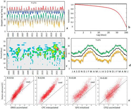
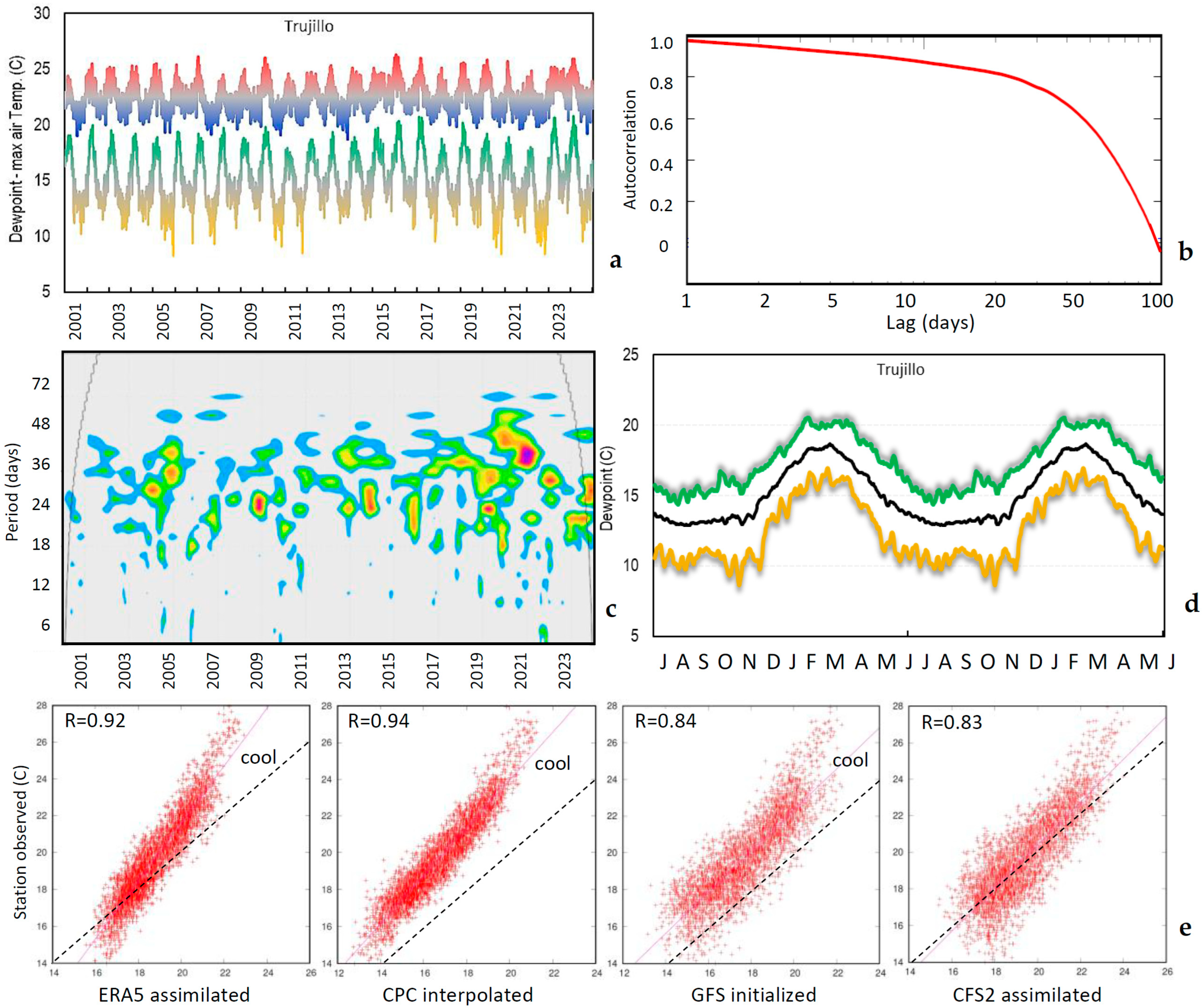
The daily ERA5 maximum and dewpoint temperature statistics are presented in Figure 3a–d. Seasonal cycling at Trujillo is evident, with maxima in the range 19–26 °C and dewpoints in the range 10–20 °C. The lag auto-correlation reveals great persistence and the wavelet spectra indicate pulsing from equatorial Madden Julian Oscillations at periods of 24–48 days [20,21,22]. The mean annual cycle of dewpoint temperature reflects ‘marine delay’, with a cool, dry winter–spring and a warm, humid summer–autumn. The dewpoint quintile range is greatest in spring, likely due to downslope winds from the Andes.
Figure 3.
(a) Daily record of ERA5 maximum air (upper) and dewpoint temperature at 8.15 S, 78.95 W. (b) Dewpoint lag auto-correlation. (c) High-frequency portion of the wavelet spectral amplitude (shaded >90% confidence). (d) Mean annual cycle ×2 of the dewpoint upper-, median, and lower- quintiles (green, black, gold). (e) Scatterplot validation of the Trujillo airport observed and model daily air temperatures (2001–2024) from (left to right): ERA5, CPC, GFS, and CFS2, note x-axis varies, the dashed line is 1:1 fit, R value and bias are listed, model record is 8765.
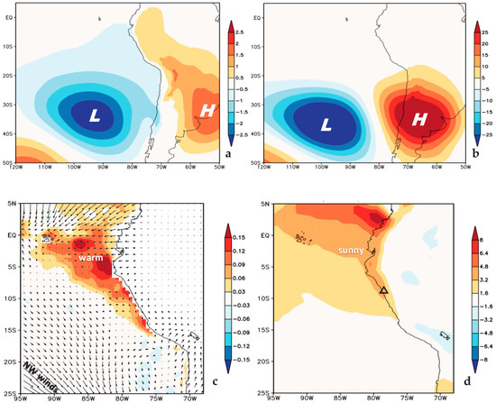
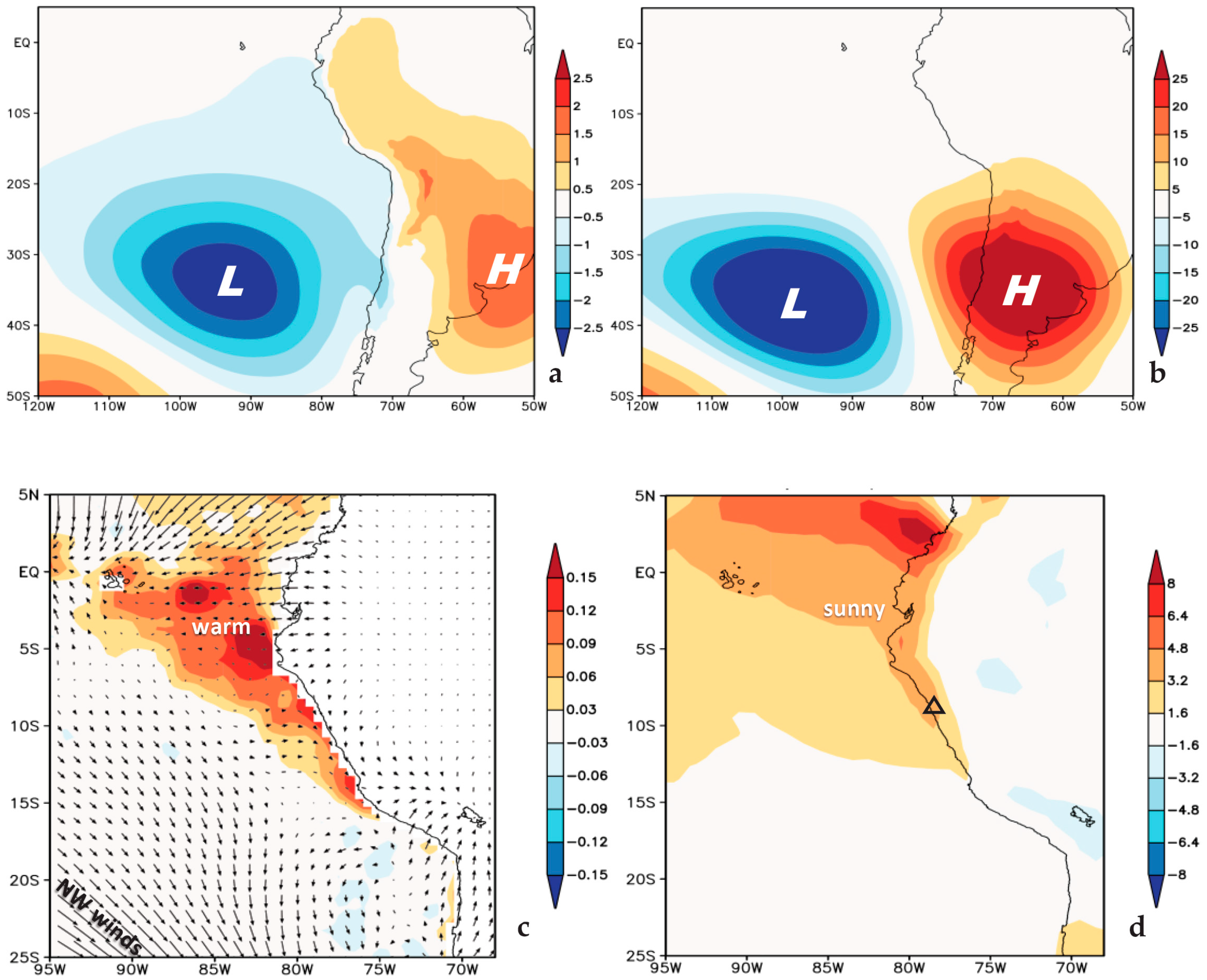
Scatterplot validations are made with Trujillo airport observations and the nearest grid-point model products (Figure 3e). Simultaneous correlations are high for ERA5 assimilation and CPC interpolation (0.92–0.94) and lower for GFS initialization and CFS2 assimilation (0.83–0.84). Three models show a cool bias at higher temperatures, but relatively good match-up at cooler temperature. Regressions of the high-pass filtered maximum temperature time series onto winter fields are presented in Figure 4a–d. Sea-level air pressure and 500 hPa geopotential height maps show that anomalous warm winter weather is associated with a baroclinic trough/ridge pattern in the subtropical westerlies (30–40 S) that weakens the southeast Pacific anticyclone and associated wind-driven upwelling. The warmer seawater inhibits low-level clouds; sunny weather prevails and the coastal plains undergo diurnal heating. The opposing pattern naturally leads to cooler, foggier conditions along the coast of Peru, as noted by [3]. Thus, tropical influences are minimal during austral winter; the main driver of anomalous temperatures is a weakening of the marine high and coastal upwelling in response to the subtropical trough/ridge pattern.
Figure 4.
Regression of 2001–2024 high-pass filtered daily maximum temperature time series onto June–August fields of (a) sea-level air pressure (hPa) with weather icons, (b) 500 hPa geopotential height (m) with weather icons, (c) sea surface temperature (C) and wind (largest vector 2 m/s), and (d) net OLR (W/m2); patterns underlying anomalous warm winter weather at Trujillo, N = 2191, neutral values are unshaded.
3.3. Temperature Gradient
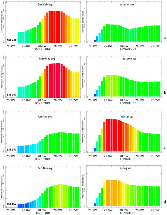
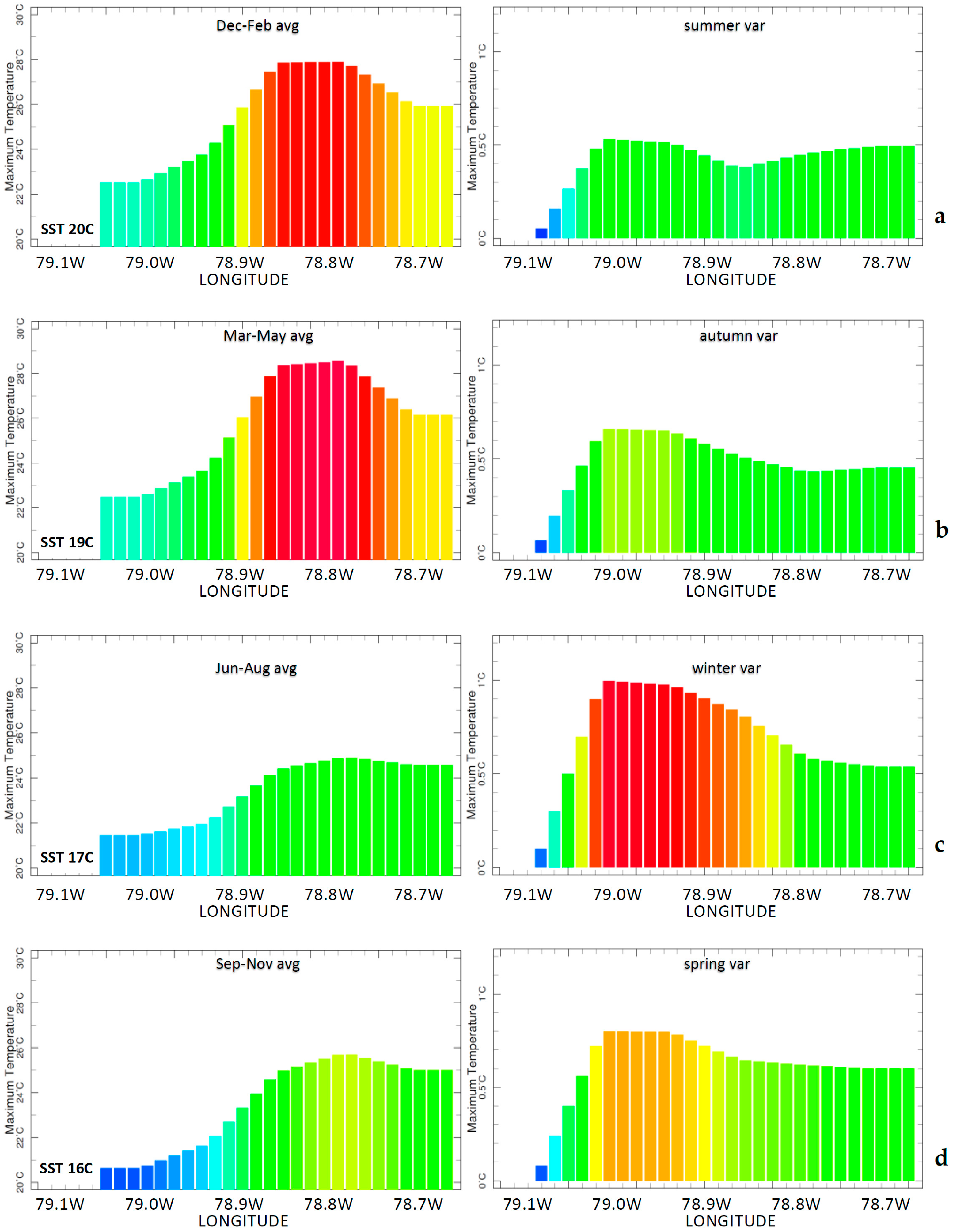
Seasonal maximum air temperature gradients on the 8.15 S transect are presented in Figure 5a–d. The increase in temperature from beachfront to coastal plains is ~5 °C/10 km, slightly steeper in summer than winter. The gradient is maintained by persistent upwelling, channeling of airflow, and tropical heat fluxes. Inter-annual variance across the transect crests 10–15 km inland and shows the highest values in winter–spring (0.8–1.0 °C)—but what are the controls and impacts?
Figure 5.
Seasonal maximum air temperature on the transect 8.15 S: (a) summer, (b) autumn, (c) winter, (d) spring; (left) average, (right) root mean square anomaly (variance); based on SENAMHI interpolation 2001–2024, each bar is 2 km width.
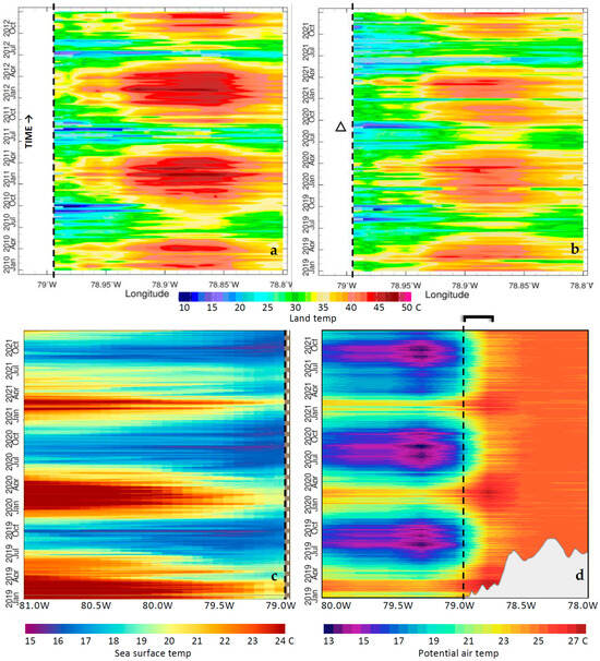
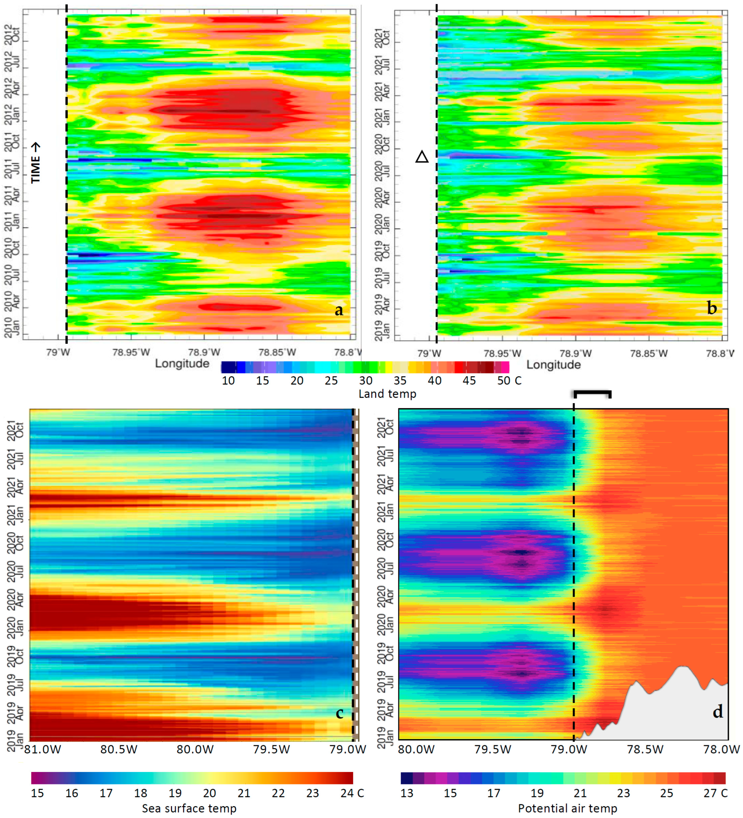
Hovmoller analyses of daily land surface, sea surface, and potential (air) temperature are plotted across the transect in Figure 6a–d. Therein, seasonal cycles and intra-seasonal pulsing emerge, as equatorial troughs alter the SE Pacific anticyclone and wind-driven coastal upwelling. The period 2010–2012 exhibited amplified warming compared with 2019–2021. There is summer relaxation and winter intensification of the cross-shore gradient. Thus June–August air temperature forecasts would need to distinguish beachfront from coastal plains and vegetated river valleys from desert landscapes. Among the temporal statistics, certain cases are noted for detailed analysis.
Figure 6.
Hovmoller plots of weekly daytime land temperature: (a) 2010–2012, (b) 2019–2021, with case study indicated by triangle. Hovmoller plots 2019–2021 of daily (c) sea surface temperature and (d) potential air temperature with a topographic profile (lower right), all on the transect 8.15 S. Note differing longitudes and color scales, dashed line is coast, bracket refers to upper transect coverage.
3.4. Winter Case Studies
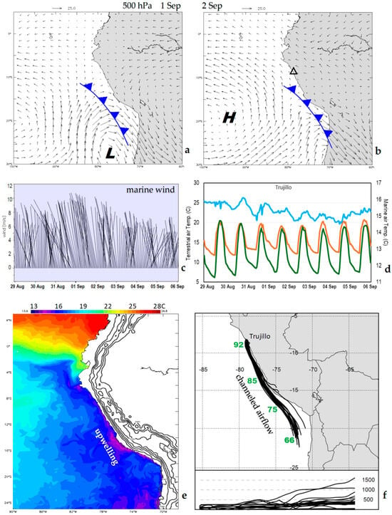
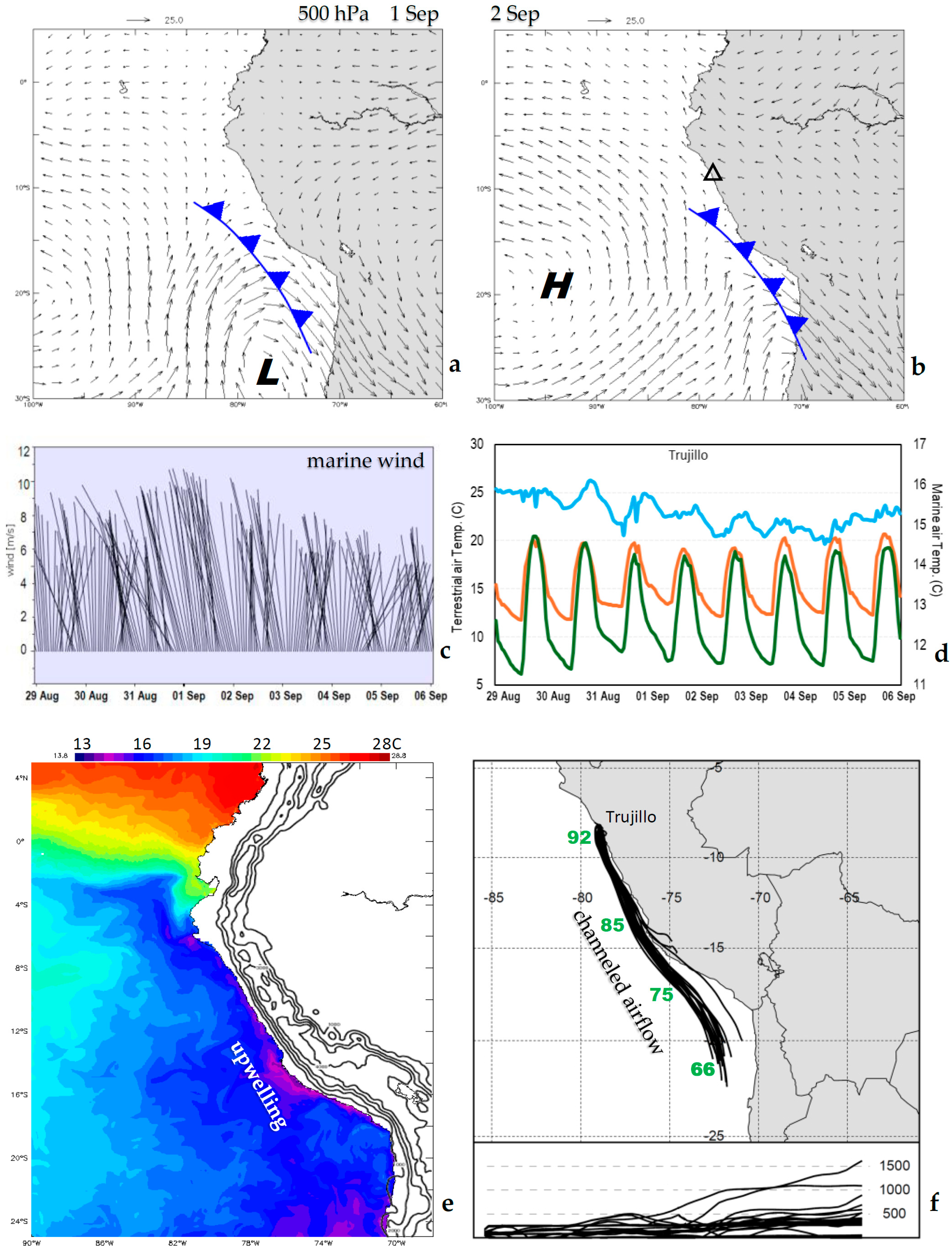
Our first case study is a cold spell at Trujillo during spring 2020 (Figure 7a–f). A subtropical trough reached northward from Chile followed by a ridge which accelerated the SSE wind > 10 m/s and coastal upwelling. Air temperatures over the sea declined to 15 °C from 1 to 4 September 2020; further inland, the hourly temperatures oscillated from 7 to 20 °C. Subsiding airflow trajectories were channeled over 14 C seawater, thus the relative humidity increased from 66 to 92%, leading to dense fog-stratus and cool weather at Trujillo.
Figure 7.
Cold spell case: (a,b) 500 hPa winds on 1 and 2 September 2020. Hourly CFS2-assimilated values: (c) Marine wind vectors near Trujillo. (d) Air temperature at sea (blue), coast (brown), and inland (green) locations on 8.15 S. (e) Sea surface temperature with topography. (f) Airflow back-trajectories during 1–3 September 2020 arriving at 100 m over Trujillo. Plan and side view (lower), with green humidity values.
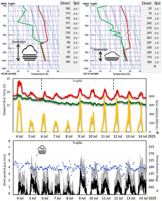
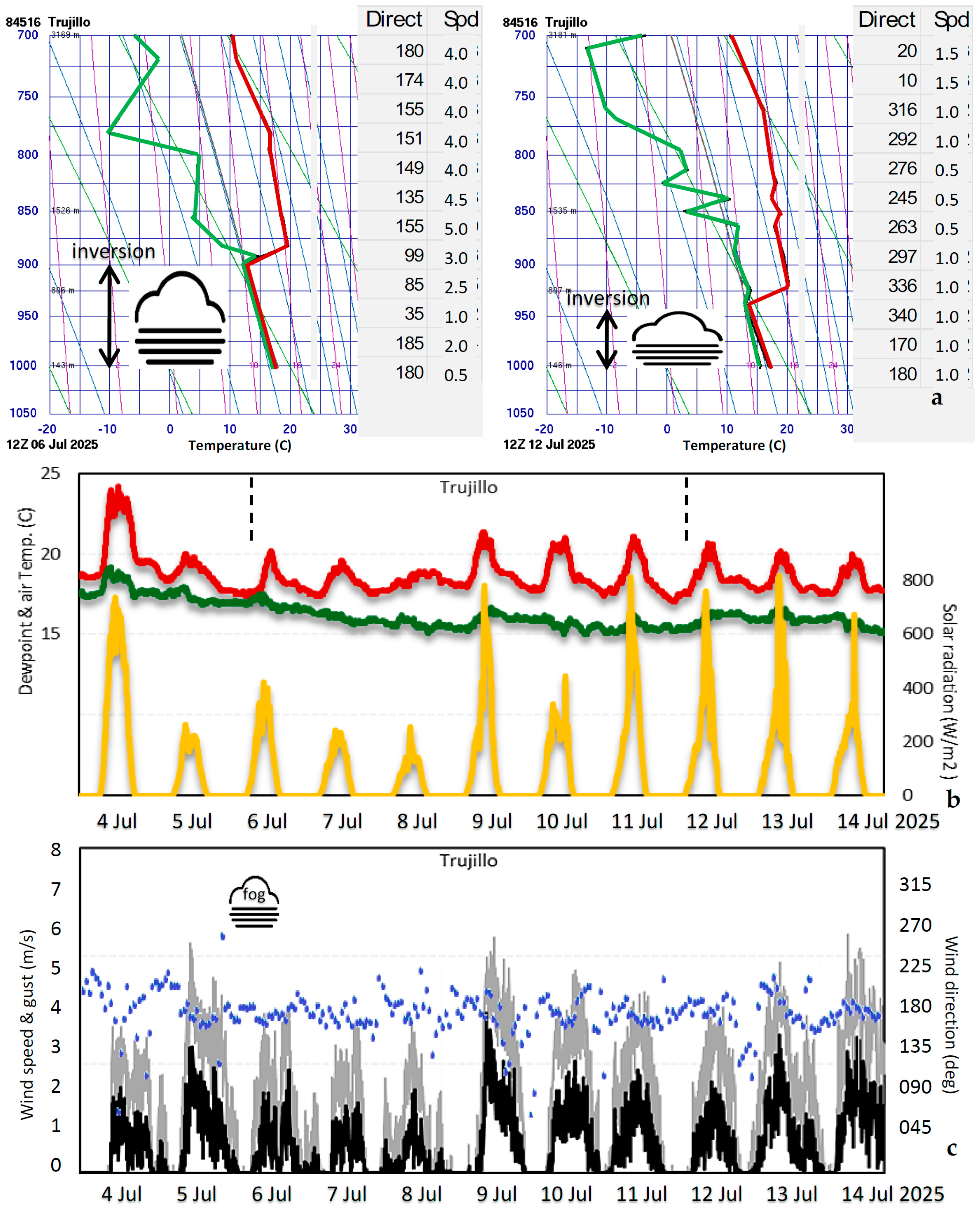
Our second case study employs in situ observations to describe an unusual winter weather scenario (Figure 8a–c). Radiosonde profiles on 6 and 12 July 2025 reveal two distinct conditions: a deep marine layer with SSE winds (6th) and a shallow marine layer with light winds (12th). Hourly weather station measurements indicate T = Td on the morning of 6 July; the radiosonde confirms a depth of 1000 m. Over 5 mm of fog-induced rain was observed at Trujillo, which may seem trivial, but the long-term July average is 0.3 mm/month. In contrast, the 12 July radiosonde profile had a moist layer depth of 500 m. The station time series exhibits a gradually declining dewpoint with solar radiation peaks > 700 W/m2. Surface measurements reveal steady SSE winds with diurnal strengthening on sunny days. There is a synergy between cloud depth and sensible heat flux which alters the advance and retreat of morning fog and air temperature gradients.
Figure 8.
(a) Radiosonde profiles at Trujillo in deep (left) and shallow morning fog, temperature (red), dewpoint (green), direction, and speed (m/s) listed at right. Automatic weather station observations: (b) air and dewpoint temperature (red, green) and solar radiation (gold) with radiosonde dates dashed, (c) wind speed and gust and wind direction (blue dots); fog-rain (5 mm) occurred on 6 July 2025.
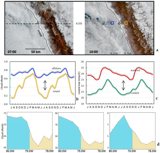
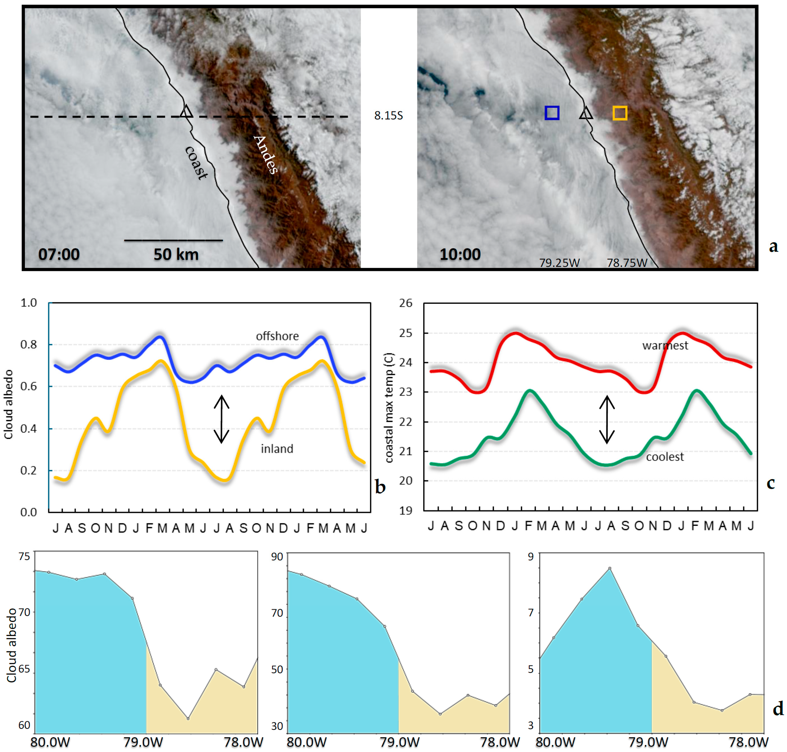
These features are analyzed via a third case study using satellite remote sensing in Figure 9a. Visible imagery on a typical winter morning (07:00) reveals shallow clouds advancing ~10 km inland to the Andes, then retreating to the coast by 10:00 h. The seasonality of fog-stratus penetration is analyzed in the context of maximum temperature in Figure 9b. At the marine location (79.25 W) the median satellite cloud albedo remains high all year (62–83%), whereas inland (78.75 W) winter is sunny (17%). This affects the inter-annual range of maximum temperature at the coast (79.0 W), which is greatest in winter (3 °C) and thus prone to forecast errors caused by the variable penetration of marine fog-stratus. Analyzing the average and standard deviation of cloud albedo along the transect (Figure 9c), there is a steep gradient, especially during winter (80% sea, 35% land) and the greatest variance is near the beachfront.
Figure 9.
(a) Visible GOES satellite imagery with fog advancing and retreating during (July 2025) on an early winter morning, station—triangle. Mean annual cycle ×2 of (b) inland (gold) and offshore (blue) cloud albedo (at grid-points upper right) and (c) coastal maximum temperatures of the high (red) and low (green) quintile; arrows refer to greatest range. (d) Cloud albedo on the transect 8.15 S, left to right: all-year average, June–August average, and June–August standard deviation; blue/tan shading distinguishes sea/land.
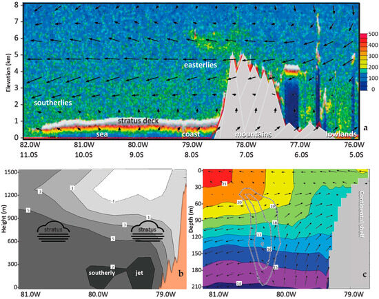
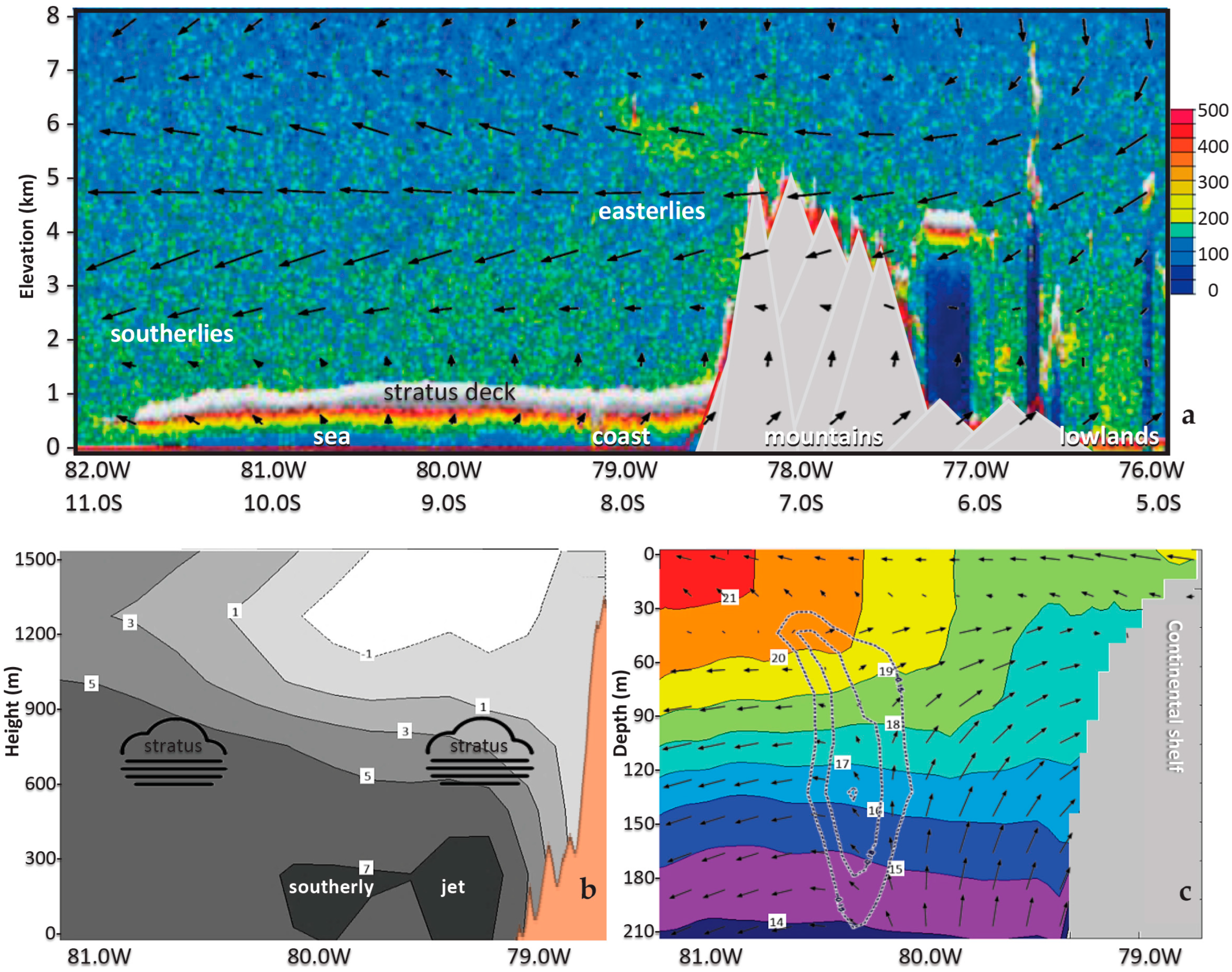
The fourth case study utilizes a satellite lidar aerosol height-section during winter (Figure 10a). There is a fog-stratus deck of a uniform ~1 km height extending seaward, confined by subsidence from above and cooling from below. Easterlies of 7 m/s flow across the Andes Mountains at 3–5 km elevation, above a dense aerosol layer (500 µg/m3). Analyzing a cross-section during this time (13 July 2008, Figure 10b,c), a shallow 7 m/s southerly jet occurs within 100 km of the coast [23]. Offshore Ekman transport in the upper ocean drives upwelling over the shelf west of Trujillo. An undercurrent diverts the uplifted seawater and helps maintain strong sea temperature gradients.
Figure 10.
(a) Satellite lidar backscatter (0.532 µm) during an early winter morning (13 July 2008); aerosol density (µg/m3) with zonal circulation vectors (largest 7 m/s) and labels. Cross-section of the transect west of Trujillo on 13 July 2008: (b) lower atmosphere meridional wind, (c) upper ocean temperature, zonal circulation (vectors) with vertical motion exaggerated 30-fold, and southward undercurrent (<−0.15 m/s dashed).
4. Concluding Discussion
This study has evaluated coastal temperature gradients over recent decades near Trujillo, Peru, (8.15 S, 79 W) using high-resolution data assimilation. A cross-shore transect was analyzed for seasonality of maximum temperature using SENAMHI interpolated measurements compared with downscaled ERA5 reanalysis. Statistical outcomes found a 5 °C/10 km increase from the cool beachfront to the warm plains below the Andes. Controlling factors include the following processes: wind-driven upwelling → low cloud cover → net solar radiation → sensible heat flux → inland warming. Heat flux data (cf. Figure 2c) was used in a boundary layer 300 m deep over 6 h/day, from the thermodynamic equation ΔT = SHF dt/M Cp = 80 W/m2 (2.16 × 10⁴ s)/360 kg (103 J/kg °C) = 4.8 °C. Sharp gradients in fog-stratus and net solar radiation caused by SSE-channeled wind maintain a steep gradient of maximum temperature.
Short-range weather forecasts for Trujillo had a cool bias and under-represent the steep temperature gradient induced by coastal upwelling in tropical latitudes. Fluctuations in the diurnal cycle of turbulent heating (cf. Figure 1c) depend on the depth, inland penetration, and duration of morning fog-stratus. Although seasonality is limited by persistent SSE winds, the greatest range of cloud albedo and maximum temperature occurs during winter (cf. Figure 5c and Figure 9b), when forecast errors are most likely. Regressions of temperature time series onto meteorological fields identify that a subtropical trough/ridge pattern in 30–40 S latitudes contributes to higher winter values associated with weaker upwelling and sunny weather at Trujillo, Peru, (8 S).
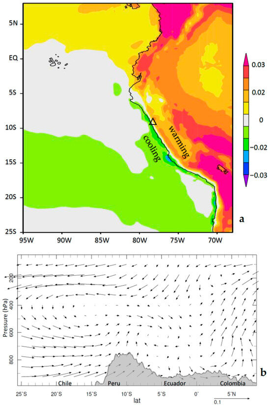
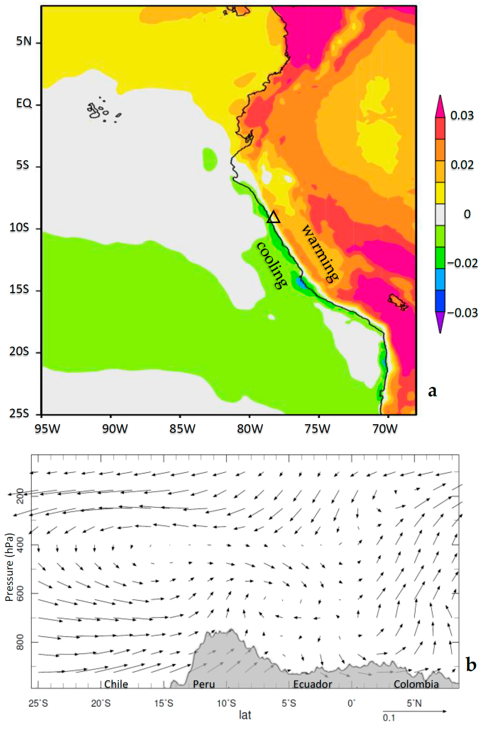
Long-term trends 1980–2024 show intensified upwelling and cooler sea temperatures [24], in contrast with the warmer coastal plains and interior (Figure 11a). These changes involve an acceleration of long-shore winds by the southern Hadley Cell (Figure 11b). Assuming persistence, the growing contrast between the cool beachfront and warm uplands offers the benefit that populations can shift to optimize human comfort and adapt to climate change.
Figure 11.
Climatic trend analysis 1980–2024: (a) ERA5 air temperature (C/yr) and (b) meridional (Hadley) circulation averaged 82–76 W, with topographic profile (m s−1/yr).
Funding
This research received no external funding.
Data Availability Statement
The original contributions presented in this study are included in the article. Further inquiries can be directed to the corresponding author.
Acknowledgments
N. Zamudio-Espinoza of SENAMHI Peru promoted this topic for study at a workshop hosted by the National University of Trujillo in July 2025. The websites used for data analysis include APDRC University Hawaii, Iowa Enviro-monitoring, IRI Climate Library, KNMI Climate Explorer, and NOAA Ready–ARL. Outcome-based support from the South African Deparment of Higher Education via the University Zululand is acknowledged.
Conflicts of Interest
The author declares no conflicts of interest.
References
- Garreaud, R.; Muñoz, R.C. The low-level jet off the west coast of subtropical South America: Structure and variability. Mon. Weather Rev. 2005, 133, 2246–2261. [Google Scholar] [CrossRef] [Scilit]
- Rau, P.; Bourrel, L.; Labat, D.; Melo, P.; deWitte, B.; Frappart, F.; Lavado, W.; Felipe, O. Regionalization of rainfall over the Peruvian Pacific slope and coast. Int. J. Climatol. 2017, 37, 143–158. [Google Scholar] [CrossRef] [Scilit]
- Aliaga-Nestares, V.; De La Cruz, G.; Takahashi, K. Comparison between operational and statistical daily maximum and minimum temperature forecasts on the central coast of Peru. Weather Forecast. 2023, 38, 555–570. [Google Scholar] [CrossRef] [Scilit]
- Illig, S.; Dewitte, B.; Goubanova, K.; Cambon, G.; Boucharel, J.; Monetti, F.; Flores, R. Forcing mechanisms of intraseasonal SST variability off central Peru in 2000–2008. J. Geophys. Res. Ocean. 2014, 119, 3548–3573. [Google Scholar] [CrossRef] [Scilit]
- Cai, W.; McPhaden, M.J.; Grimm, A.M.; Rodrigues, R.R.; Taschetto, A.S.; Garreaud, R.D.; Vera, C. Climate impacts of the El Niño–Southern Oscillation on South America. Nat. Rev. Earth Environ. 2020, 1, 215–231. [Google Scholar] [CrossRef] [Scilit]
- Huaman, L.; Schumacher, C.; Kiladis, G. Eastward-propagating disturbances in the tropical Pacific. Mon. Weather Rev. 2020, 148, 3713–3728. [Google Scholar] [CrossRef] [Scilit]
- Jury, M.R.; Alfaro-Garcia, L. Peru north coast climate variability and regional ocean-atmosphere forcing. Coasts 2024, 4, 508–534. [Google Scholar] [CrossRef] [Scilit]
- DeWitte, B.; Illig, S.; Renault, L.; Goubanova, K.; Takahashi, K.; Gushchina, D.; Mosquera, K.; Purca, S. Modes of covariability between sea surface temperature and wind stress intraseasonal anomalies along the coast of Peru from satellite observations (2000–2008). J. Geophys. Res. 2011, 116, C04028. [Google Scholar] [CrossRef] [Scilit]
- Espinoza, J.C.; Ronchail, J.; Lengaigne, M.; Quispe, N.; Silva, Y.; Bettolli, M.L.; Avalos, G.; Llacza, A. Revisiting wintertime cold air intrusions east of the Andes: Propagating features from subtropical Argentina to Peruvian Amazon and relationship with large-scale circulation patterns. Clim. Dyn. 2013, 41, 1983–2002. [Google Scholar] [CrossRef] [Scilit]
- Quispe-Gutiérrez, N.; Aliaga-Nestares, V.; Rodríguez-Zimmermann, D.; Bonshoms, M.; Loayza, R.; García, T.; Mesia, J.; Duran, R.; Olivares, S. Cutoff low over the southeastern Pacific Ocean: A case study. J. South. Hemisph. Earth Syst. Sci. 2021, 71, 17–29. [Google Scholar] [CrossRef] [Scilit]
- Huerta, A.; Aybar, C.; Imfeld, N.; Correa, K.; Felipe-Obando, O.; Rau, P.; Lavado-Casimiro, W. High-resolution grids of daily air temperature for Peru–the new PISCOt v1.2 dataset. Sci. Data 2023, 10, 847. [Google Scholar] [CrossRef] [Scilit]
- Saha, S.; Moorthi, S.; Wu, X.; Wang, J.; Nadiga, S.; Tripp, P.; Behringer, D.; Hou, Y.-T.; Chuang, H.-Y.; Iredell, M.; et al. The NCEP Climate Forecast System version 2. J. Clim. 2014, 27, 2185–2208. [Google Scholar] [CrossRef] [Scilit]
- Chen, M.; Shi, W.; Xie, P.; Silva, V.B.; Kousky, V.E.; Higgins, R.W.; Janowiak, J.E. Assessing objective techniques for gauge-based analyses of global daily precipitation [and temperature]. J. Geophys. Res. 2008, 113, D04110. [Google Scholar]
- Hersbach, H.; Bell, B.; Berrisford, P.; Hirahara, S.; Horányi, A.; Muñoz-Sabater, J.; Nicolas, J.; Peubey, C.; Radu, R.; Schepers, D.; et al. The ERA5 global reanalysis. Qtr. J. R. Meteorol. Soc. 2020, 146, 1999–2049. [Google Scholar] [CrossRef] [Scilit]
- Environmental Modelling Center (NOAA). The GFS Atmospheric Model; National Centers for Environmental Prediction: College Park, MA, USA, 2004; Volume 442, p. 14. [Google Scholar]
- Chassignet, E.P.; Hurlburt, H.E.; Metzger, E.J.; Smedstad, O.M.; Cummings, J.A.; Halliwell, G.R.; Bleck, R.; Baraille, R.; Wallcraft, A.J.; Lozano, C.; et al. US GODAE: Global ocean prediction with the Hybrid coordinate ocean model. Oceanography 2009, 22, 64–75. [Google Scholar] [CrossRef] [Scilit]
- Winker, D.M.; Hunt, W.M.; McGill, M.J. Initial performance assessment of CALIOP. Geophys. Res. Lett. 2007, 34, L19803. [Google Scholar] [CrossRef] [Scilit]
- Hulley, G.; Freepartner, R.; Malakar, N.; Sarkar, S. MODIS Land Surface Temperature and Emissivity Product v6; NASA-GSFC-JPL: Pasadena, CA, USA, 2022. [Google Scholar]
- Jury, M.R.; Gaviria Pabón, A.R. Dispersion of smoke plumes over South America. Earth Interact. 2021, 25, 1–14. [Google Scholar] [CrossRef] [Scilit]
- Roundy, P.E.; Kiladis, G.N. Observed relationships between oceanic kelvin waves and atmospheric forcing. J. Clim. 2006, 19, 5253–5272. [Google Scholar] [CrossRef] [Scilit]
- Rydbeck, A.V.; Jensen, T.G.; Flatau, M. Characterization of intra-seasonal Kelvin waves in the equatorial Pacific Ocean. J. Geophys. Res. Ocean. 2019, 124, 2028–2053. [Google Scholar] [CrossRef] [Scilit]
- Recalde-Coronel, G.C.; Zaitchik, B.; Pan, W.K. Madden–Julian oscillation influence on sub-seasonal rainfall variability on the west of South America. Clim. Dyn. 2020, 54, 2167–2185. [Google Scholar] [CrossRef] [Scilit]
- Chamorro-Gomez, A.; Colas, F.; Echevin, V.; Tam, J. Characterization of coastal jets over the Peruvian sea using the WRF regional model. Bol. Inst. Mar Peru 2022, 37, 271–284. [Google Scholar]
- Bakun, A.; Black, B.A.; Bograd, S.J.; Garcia-Reyes, M.; Miller, A.J.; Rykaczewski, R.R.; Sydeman, W.J. Anticipated effects of climate change on coastal upwelling ecosystems. Curr. Clim. Change Rep. 2015, 1, 85–93. [Google Scholar] [CrossRef] [Scilit]

Disclaimer/Publisher’s Note: The statements, opinions and data contained in all publications are solely those of the individual author(s) and contributor(s) and not of MDPI and/or the editor(s). MDPI and/or the editor(s) disclaim responsibility for any injury to people or property resulting from any ideas, methods, instructions or products referred to in the content. |
© 2026 by the author. Licensee MDPI, Basel, Switzerland. This article is an open access article distributed under the terms and conditions of the Creative Commons Attribution (CC BY) license.