


Abstract
Evaluating conflicting early-stage design objectives, such as minimizing area-normalized cooling energy intensity (kWh/m2) and maximizing spatial Daylight Autonomy under static shading (sDA300/50%), is limited by the computational cost of building performance simulation. This study develops Random Forest surrogate models of Honeybee (EnergyPlus and Radiance) simulations for single-zone offices in the hot arid climate of Cairo, trained on 1037 parametric scenarios generated with a hybrid sampling strategy. In 10-fold cross-validation, the models reproduced the simulated cooling and heating intensities and four climate-based daylight metrics with an R2 of 0.943–0.990 and mean absolute percentage errors below 4% for all indicators except Annual Sunlight Exposure (7.9%), while reducing the evaluation time from about 55 s per simulation to about 0.3 s. Room depth and window-to-wall ratio were the most influential variables overall, and orientation dominated sunlight exposure. A surrogate-assisted multi-objective optimization, verified by 124 additional full simulations, showed that the surrogate overestimates daylight performance at the extremes of the design space; the verified Pareto front indicates that north- to north-east-facing rooms with the baseline glazing achieve an sDA above 90% at about 119 kWh/m2. The surrogate, deployed in an interactive tool, is best used for rapid screening, with final candidates confirmed by simulation.
1. Introduction
Buildings contribute significantly to energy demand, accounting for around 29% of total energy consumption [1] and greater than 41% of primary energy consumption in developed settings like the United States [2]. Modern architectural practices implemented to minimize this massive energy footprint rely on building performance simulation (BPS) tools at the earliest stages of building conceptual design to assess their energy efficiency and indoor environmental quality. However, traditional physics-based BPS methods face significant challenges due to their high computational cost and time consumption [3]. This restriction delays the iterative analysis of thousands of design options and the integrated execution of multi-objective optimization (MOO), leading to slower decision-making in target exploration [4].
To alleviate these computational bottlenecks, data-driven surrogate models based on machine learning (ML) algorithms have emerged as efficient alternatives. A surrogate model learns the relationship between design parameters and simulated performance from a set of simulation results and then predicts the performance of new design options almost instantly. This allows architects to explore and optimize the design space at a fraction of the computational cost of simulation [3,5]. ML algorithms used as building-performance surrogates belong to a few main families: linear regression; kernel-based methods, such as support vector regression (SVR) and Gaussian process regression; instance-based methods, such as k-nearest neighbours (KNN); artificial neural networks (ANNs), ranging from multilayer perceptrons to generative and graph networks recently applied to daylight and energy prediction; and tree-based ensembles, which combine many decision trees either by averaging independently grown trees (bagging, e.g., Random Forest) or by fitting trees sequentially to the remaining errors (boosting, e.g., gradient boosting and XGBoost) [3,4,6,7,8]. Representatives of these families are compared on the dataset of this study in Appendix A.
Even with considerable progress in surrogate modelling, several important research gaps still exist. Given its complex nature and the trade-offs between thermal performance and visual comfort [9], single-objective optimizations have been the main approach in previous studies. This challenge is particularly severe in hot arid climates, like Cairo, Egypt, where thermal cooling loads become the primary energy end-use due to high solar radiation. Such regions require shading devices to control solar heat gains [10], but shading directly competes with daylight admission [11].
Therefore, this study develops an accurate and computationally efficient surrogate model for the integrated assessment of cooling energy intensity and daylight performance in early-stage office design in Cairo, Egypt. Random Forest models are trained on 1037 parametric simulation scenarios generated with Grasshopper, EnergyPlus, and Radiance using a hybrid sampling strategy [12], and together they predict area-normalized cooling and heating intensity and four climate-based daylight metrics (sDA, mean DA, mean UDI, and ASE). The study contributes (i) a surrogate framework that couples energy and multi-metric daylight prediction for a hot arid office context, (ii) a quantitative account of the non-linear trade-offs among glazing ratio, shading, and orientation in that context, and (iii) a benchmark of eight regression algorithms, together with an assessment of the sensitivity of the results to the room’s position within a building. The trained models are deployed in an interactive decision-support tool that gives architects immediate feedback on these trade-offs without requiring programming knowledge.
2. Literature Review
2.1. The Computational Challenge in Building Performance Simulation
In the design phase, building performance simulation (BPS) tools are important to verify building energy efficiency and indoor environmental quality. Nonetheless, the need for fast speed and computational efficiency makes it difficult to adopt traditional physics-based BPS methods [3,13]. Evaluating thousands of design variants solely through physical simulations is cumbersome in general due to the need for large computational resources, and will not suffice for rapid decision-making as architectural design optimization problems become more complex [1,4,14].
2.2. The Rise in Machine Learning-Based Surrogate Models
Data-driven surrogate models have emerged as efficient alternatives to address the computational challenges faced by conventional BPS [4,8]. This is done by training a mathematical model (e.g., a machine learning (ML) algorithm) to predict BPS performance data, enabling designers to run hundreds of building configurations at minimal computational cost [1,15]. Surrogate models are built by ML algorithms like artificial neural networks (ANNs), Random Forest (RF), and eXtreme Gradient Boosting (XGBoost) that use detailed physics-based simulation outputs to create approximators, which then reproduce the simulation outputs at a much lower computational cost [16,17]. Recent studies show that well-trained ML models, particularly ensemble methods (e.g., XGBoost and RF), yield instant predictions with remarkable accuracy, making them ideal for running extensive design space searches [5,7].
Indeed, the power of tree-based ensemble algorithms, specifically that of Random Forest (RF), has been corroborated by a growing number of recent studies for their ability to manage non-linear building energy datasets with little hyperparameter adjustment. Several of these studies have shown that RF is superior compared with other conventional machine learning algorithms concerning predicting heat and cooling loads, even when small training datasets are used, while retaining good accuracy [17,18]. Moreover, the incorporation of these algorithms at early stages of design improves thermal comfort and energy consumption by a considerable amount [8,19].
2.3. Multi-Objective Optimization and Trade-Offs in Building Design
Multi-objective optimization (MOO) with surrogate models represents a paradigm shift in the field of building design [9]. There exist inherent conflicting objectives when optimizing specific building components, such as shading devices and glazing properties. As an example, although deep shading solid overhangs are very effective at minimizing solar heat gains and later cooling loads, they reduce daylight access [11]. As such, robust sensitivity analyses that properly rank and assess the influence of these design variables are essential to capture non-linear trade-offs [20,21].
Additionally, recent feature-importance analyses explicitly rank fenestration and shading variables as the most influential determinants of building performance. The modelling shows that variations in solid overhang depths and glazing properties significantly influence the trade-off between overheating mitigation and daylight penetration [20,22,23,24].
2.4. Data Generation and Hybrid Sampling Strategies
The quality and predictive accuracy of a surrogate model depend heavily on its underlying training dataset; in turn, the range, distribution, sampling method, and sample size are key considerations for any development process [12]. Researchers argue that the design space must be carefully sampled to ensure that results are generalizable and robust. In contrast to many studies that rely on isolated sampling methods, such as Latin Hypercube Sampling (LHS) [4], an integrated hybrid sampling approach ensures that important regions in the design space are explored. In this way, the core geometric variables can be designed with a full factorial design, while random sampling and some targeted stress tests for certain extreme physical configurations can be used to create an effective predictive model that will generalize and capture both the trends along broad dimensions of a building’s performance as well as potentially complex, non-linear interactions without danger of overfitting [23].
2.5. Daylighting Metrics and Performance Thresholds
Climate-based daylight modelling evaluates daylight availability over a full year using hourly sky conditions derived from local weather data, rather than a single standard sky [25]. Four complementary climate-based metrics are used in this study.
Daylight Autonomy (DA300) is the percentage of occupied hours during which a point receives a minimum illuminance from daylight alone [25]; a threshold of 300 lux is used here, as in IES LM-83-12. Being a point metric, it describes daylight sufficiency at a specific location.
Useful Daylight Illuminance (UDI) is the percentage of occupied hours during which illuminance at a point falls within a range considered useful: high enough to be useful, but not so high as to risk glare or overheating [26]. Nabil and Mardaljevic originally proposed 100–2000 lux; this study adopts 100–3000 lux, the default range in the Honeybee simulation environment. Unlike DA, UDI penalizes excessive illuminance. It may therefore decrease when daylight availability increases, particularly on sun-exposed façades.
Spatial Daylight Autonomy (sDA300/50%) is the percentage of the analysis area that achieves DA300 for at least 50% of the occupied hours (08:00–18:00) [27]. IES LM-83-12 regards sDA ≥ 55% as “nominally accepted” and sDA ≥ 75% as “preferred” daylight sufficiency.
Annual Sunlight Exposure (ASE1000, 250 h) is the percentage of the analysis area receiving more than 1000 lux of direct sunlight for more than 250 occupied hours per year, computed without operable shading [27]. An ASE value not exceeding 10% is commonly used as the upper limit for acceptable visual comfort.
Of these metrics, IES LM-83-12 standardizes only sDA and ASE. DA and UDI are established research metrics that the standard does not define.
2.6. Research Gap and Contribution
The studies reviewed in Section 2.1, Section 2.2, Section 2.3 and Section 2.4 establish the individual components of the present workflow: tree-based surrogates trained on parametric simulations, feature-importance analysis, surrogate-assisted multi-objective optimization and practitioner-facing interfaces [3,4,5]. The contribution of this study therefore lies not in a new algorithm but in three aspects that these studies leave open.
First, the surrogate studies closest to this work predict thermal or energy-related objectives only: energy use and thermal comfort in office retrofits in a cold climate [5], heating and cooling loads and thermal discomfort for shading-device design [10], and indoor air temperature under the shading of surrounding urban buildings [24]. Conversely, daylight surrogates predict daylight performance alone; this applies to the multimodal model of Li et al. [6] and to the fifteen daylight surrogate studies they review. The present model predicts area-normalized cooling and heating intensity together with four climate-based daylight metrics, including the glare-related indicators ASE and UDI, from the same early-stage design variables.
Second, it addresses an office typology in a hot arid climate, where cooling dominates energy use and solar control competes directly with daylight admission, and it quantifies how strongly and how non-linearly glazing ratio, shading, and orientation govern that conflict (Section 4.1). Third, it benchmarks eight regression algorithms on the same multi-indicator dataset (Appendix A) and quantifies the sensitivity of the results to the room’s floor level and plan position within a building (Section 4.3), thereby delimiting the conditions under which a single-zone surrogate is applicable.
3. Methodology
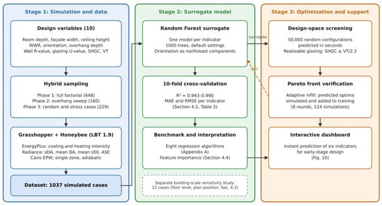
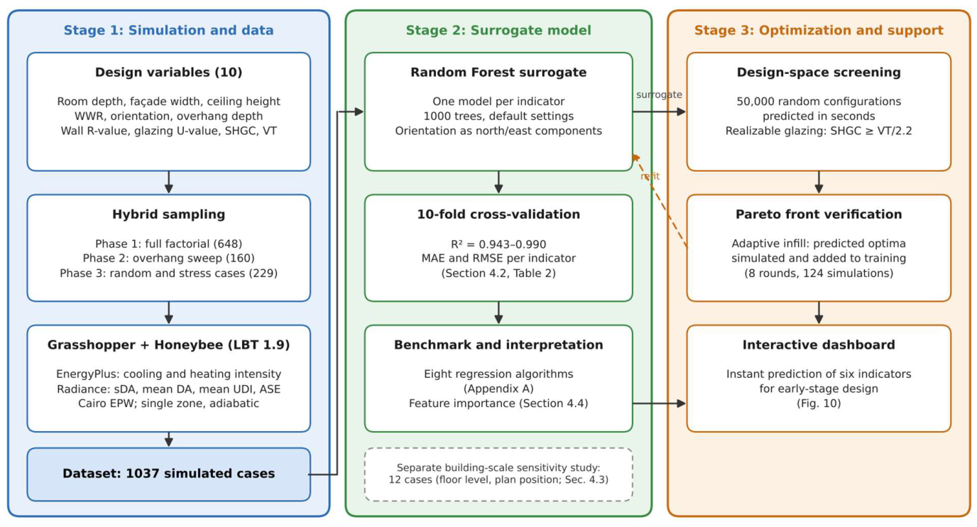
The research aims to develop a methodological framework for predicting and optimizing the integrated daylighting and thermal performance of early-stage office design. The methodology comprises three stages: (1) parametric building performance simulation (BPS) and data generation through a hybrid sampling strategy, (2) development and evaluation of the machine learning surrogate models, and (3) surrogate-assisted optimization and decision support (see Figure 1).
Figure 1.
Overall workflow of the study: (Stage 1) parametric simulation and generation of the 1037-case dataset; (Stage 2) development and cross-validation of the Random Forest surrogate models; and (Stage 3) surrogate-assisted optimization verified by simulation, and the interactive decision-support tool. The building-scale sensitivity study (Section 4.3) consists of separate simulations outside the training dataset.
3.1. Parametric Building Performance Simulation Setup
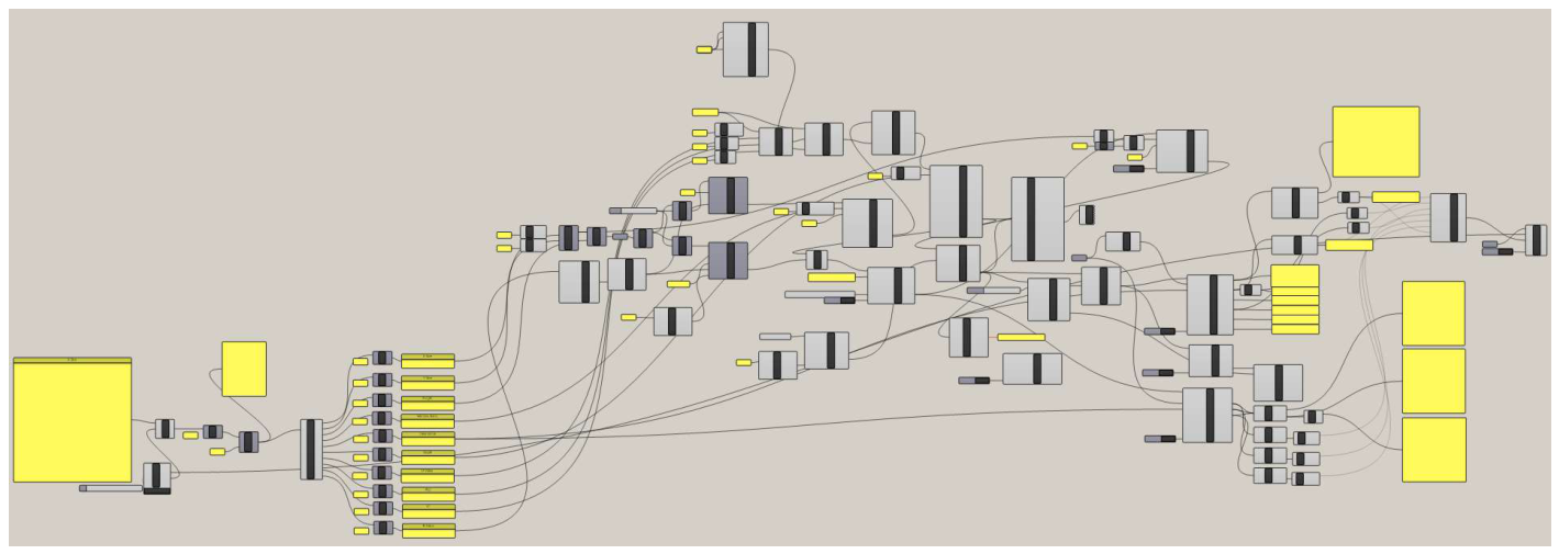
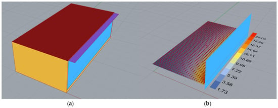
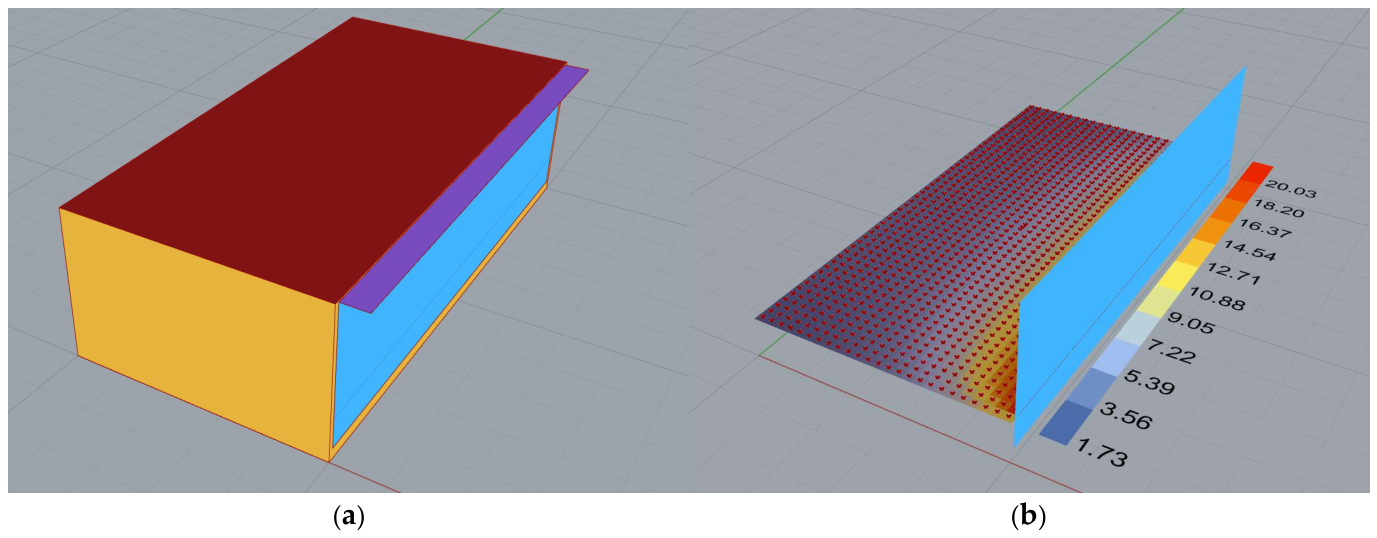
The parametric framework was developed within the visual programming environment Grasshopper for Rhinoceros 3D, and used plugins Ladybug and Honeybee to automate the BPS process (see Figure A1 in Appendix B, as well as Figure 2). To accurately consider the environmental impact, the EnergyPlus Weather (EPW) file of Cairo, Egypt, was used in the simulation. The choice of this hot, arid climate context setting is critical to increase the conflict between reducing high cooling needs and maximizing daylighting. This simulation workflow uses Honeybee and Ladybug to connect geometrical models with EnergyPlus for thermal load calculations and with Radiance for daylighting metrics, an automated approach that has been extensively used in recent building performance studies [6,24,28].
Figure 2.
Visualization of the baseline parametric office model in the Rhino 3D environment: (a) the exterior geometric configuration, including the fenestration and horizontal shading device, and (b) the daylighting analysis setup, illustrating the spatial sensor grid established at a high resolution of 0.2 m on a standard workplane height of 0.8 m for accurate spatial Daylight Autonomy (sDA) calculations.
The development of the robust parametric workflow in Grasshopper required approximately a week of intense effort (roughly 28 h) for scripting the geometry generation, material assignments, and simulation logic. To ensure adequate spatial resolution in the daylighting simulation (Honeybee/Radiance), a space sensor grid was set up at 0.2 m spacing around the model located at a normal workplane height of 0.8 m above finished floor level. This exact grid setup ensures accurate computing for each square in the entire office area regarding spatial Daylight Autonomy (sDA).
The parametric workflow was implemented in Rhinoceros 8 and Grasshopper using Ladybug Tools 1.9 (Ladybug and Honeybee), with batch execution managed by Colibri 2.0. Thermal loads were simulated with EnergyPlus and daylighting with Radiance as bundled with Ladybug Tools 1.9, both driven through Honeybee. Climatic boundary conditions were taken from the EPW file EGY_Cairo.Intl.Airport.623660_ETMY.
In Phases 1 and 2, the glazing properties were fixed, and the Radiance glazing material was the Honeybee default glass, whose visible transmittance is 0.64; VT is therefore reported as 0.64 for these cases. In Phase 3, in which the glazing properties were varied, the Radiance glass of each case was assigned a visible transmittance equal to its sampled VT. For these cases, the daylighting simulations were scripted directly with the Honeybee Python libraries of Ladybug Tools 1.9 that underlie the Grasshopper components, using the same model definition and the same Radiance build (5.4a); this scripted workflow reproduces the Grasshopper results closely (Section 4.5). VT affects only the daylighting results, because it does not enter the EnergyPlus load calculation.
Annual daylight simulations used the Honeybee enhanced two-phase daylight-coefficient recipe. In this recipe, the diffuse sky contribution is computed from hourly sky luminance distributions generated from the EPW direct-normal and diffuse-horizontal irradiance using the Perez all-weather sky model (Radiance gendaymtx), while direct sunlight is ray-traced to the actual hourly sun positions. Default Honeybee Radiance parameters were used (2 ambient bounces, 5000 ambient divisions and a limit weight of 2 × 10⁻⁵). The limited number of ambient bounces tends to underestimate inter-reflected light in deep rooms, so the reported DA and sDA values are conservative; the ASE, which depends on direct sunlight only, is not affected.
The site was modelled without surrounding buildings or other external obstructions (unobstructed context), with a ground plane reflectance of 0.2, in order to isolate the daylighting performance attributable solely to the parametric geometry under study. Occupied hours were defined as 08:00–18:00 on all days.
The four daylighting metrics are defined in Section 2.5. DA and UDI were computed with thresholds of 300 lux and 100–3000 lux, respectively. sDA and the ASE are spatial metrics, computed over the sensor grid as the percentage of sensors meeting their respective criteria, using the Honeybee Spatial Daylight Autonomy and Annual Sunlight Exposure components: DA300 was achieved for more than 50% of occupied hours for sDA, and direct illuminance above 1000 lux for more than 250 occupied hours for ASE. DA and UDI, by contrast, are point metrics evaluated at each sensor; to obtain a single value per design scenario, they were averaged over all sensors (spatial mean DA and mean UDI). Mean DA was retained alongside sDA because sDA, being a pass/fail count, saturates at 100% in 164 of the 1037 scenarios (16%), whereas mean DA continues to discriminate among them (84.9–92.9%).
Because the model contains a fixed overhang and no operable shading, the reported sDA corresponds to sDA300/50% under static shading. It does not follow the operable-blind protocol of IES LM-83-12 and is therefore not an LM-83- or LEED-compliant value. Since deploying blinds generally reduces interior illuminance, the reported values should be read as an upper bound of the LM-83 sDA, particularly for orientations with high ASE. ASE, in contrast, is consistent with the LM-83-12 definition, which requires it to be evaluated with all operable shading devices retracted.
For surfaces not explicitly assigned custom optical properties, the default Honeybee Radiance modifiers were applied: a visible reflectance of 0.35 for the horizontal overhang (generic exterior shade) and 0.50 for the glazed façade wall (generic wall). The remaining room surfaces were assigned a custom visible reflectance of 0.5, and the ground plane a reflectance of 0.2 (Table 1).
Table 1.
Parametric simulation variables defining the architectural design space, including geometric configurations, shading dimensions, and thermophysical properties, with their primary discrete values and the extended ranges used for the hybrid sampling strategy (N = 1037).
The baseline model is a generic single-zone office building. To cover the design space extensively, 10 independent design variables were selected. These include geometric features (X-size, Y-size, height, orientation, and window-to-wall ratio) and physical properties (wall R-value, horizontal solid overhang depth, glass U-value, the solar heat gain coefficient (SHGC), and visible transmittance (VT)). Room depth (X-size) is the dimension perpendicular to the glazed façade, and façade width (Y-size) the dimension parallel to it. Orientation is given as the rotation of the north direction in Honeybee; with this convention, the glazed façade faces east at 0°, south at 90°, west at 180°, and north at 270°, and in the analysis it is represented by the north and east components of the window normal (Section 3.3).
The horizontal solid overhang was parametrically linked to the window geometry rather than the full façade, extending across the width of the window aperture only and scaling dynamically as the WWR varied across the sampled design space.
The recess of the glazing in the wall was represented in the thermal model by a window frame (width 0.05 m, conductance 3 W/m2K) with an outside projection of 0.1 m, which shades the glazing in the EnergyPlus solar calculation. The walls themselves were modelled as surfaces without geometric thickness, a common simplification in early-stage parametric studies, because in EnergyPlus the thermal performance of a wall is defined by its construction (R-value) rather than by its drawn thickness. In the daylighting model, the window is flush with the façade, so the daylight metrics correspond to a thin-wall façade and may be slightly higher than for a deep window reveal.
3.2. Data Generation and Hybrid Sampling Strategy
The accuracy of a surrogate model is highly dependent on the size and representativeness of its training data, but traversing all design space combinations can result in an exponential computational explosion [4,12]. In response, this study introduces a tailored hybrid sampling strategy to produce a robust dataset comprising 1037 simulation instances that achieve comprehensive design-space coverage without compromising on computational feasibility. The sampling protocol followed three strategic phases (see Table 1).
Phase 1: Full Factorial Design of Core Geometry (648 cases)
First, a baseline matrix was created that focused solely on geometric combinations (dimensions, heights, orientations, and WWRs) as static with constant physical material and shading depths (e.g., wall R-value = 3.5 and solid overhang depth = 0.3 m). This step allows the basic relationships between the building’s physical form and its energy/daylight reactions to be captured without complications from different materials.
Phase 2: Targeted Component Variations (160 cases)
Targeted sweeps were performed to examine the isolated contribution of crucial building envelope components. For example, results were obtained by testing shading devices with variations in horizontal solid overhang depths ranging from 0.0 m to 1.8 m at different orientations as well as WWRs. This variation was targeted because the model must learn the complex, non-linear relationships underlying shading design decisions over a building’s lifetime: a shading device has to block direct sunlight (to minimize cooling loads) while still admitting daylight [11]. In this phase, a 6 × 6 × 3 m room with the baseline envelope was simulated for four orientations, four WWRs (0.2–0.8), and ten overhang depths (0.0–1.8 m), giving 160 cases; the envelope and glazing properties were varied only in Phase 3.
Phase 3: Stress Tests and Randomized Sampling (229 cases)
To improve the robustness of the surrogate model and prevent overfitting, “corner cases” and extreme configurations were included in the dataset. These behaviours were tested on irregular dimensions (e.g., extremely shallow or narrow corridors), slanted orientations (e.g., 22.5° and 67.5°), and fully randomized combinations of all 10 variables. Applying randomized stress tests is consistent with standard model validation procedures, where the resultant model shows high generalizability and can effectively assess unconventional architectural configurations on unseen data [12].
The adequacy of the sample size was checked with a learning curve. The 10-fold cross-validation described in Section 3.3 was repeated with the Random Forest trained on random subsets of 20%, 40%, 60%, and 80% of each training fold. The mean cross-validated R2 of the six indicators rose from 0.886 with 187 training cases to 0.957 with 560 and 0.976 with all 933, and the last increase, from 747 cases, was only 0.006. Additional cases would therefore improve accuracy only marginally, mainly for UDI (R2 0.925 to 0.941). The dataset also far exceeds the common guideline of about ten runs per input variable for computer experiments [29].
3.3. Surrogate Model Development
After the 1037 cases had been simulated, a Random Forest regressor was trained to serve as a rapid performance predictor, an approach that has been shown to handle complex architectural datasets with accuracy competitive with the underlying simulations at a fraction of their computational cost [5]. A separate Random Forest was trained for each of the six performance indicators, using 1000 trees and otherwise the default hyperparameters of scikit-learn 1.9 (all features considered at each split, a minimum of one sample per leaf, bootstrap sampling; random_state = 42). The ten design variables formed the input, with orientation encoded by the north and east components of the window normal (the cosine and sine of the window azimuth), because orientation is a circular variable. Model accuracy was evaluated by 10-fold cross-validation with shuffled folds, which uses every case once for testing and is less sensitive to the closely related cases of the full-factorial and targeted-sweep phases than a single random split. The models used in the decision-support tool were then trained on all 1037 cases.
To justify the choice of algorithm, Random Forest was benchmarked against seven other regression algorithms commonly used for building-performance surrogates: Extra Trees, XGBoost, Gradient Boosting, a multilayer perceptron (MLP), support vector regression (SVR), k-nearest neighbours (KNN), and multiple linear regression. All models were evaluated with 10-fold cross-validation using identical folds and the same eleven input features (the ten design variables, with orientation encoded by its north and east components), with default library hyperparameters (scikit-learn 1.9 and XGBoost 3.4), so that no algorithm benefited from selective tuning. The only exception is the number of trees of the Random Forest, which was set to 1000, as in the surrogate model. For MLP, SVR, and KNN, inputs and outputs were standardized within each training fold, and the MLP iteration limit was raised to 3000 to ensure convergence.
Throughout this paper, the term “accuracy” refers to the agreement between the surrogate predictions and the EnergyPlus/Radiance simulation outputs on which the model was trained and tested. The parametric simulation model itself was not calibrated against measured data; therefore, the absolute accuracy of the predictions is bound by that of the underlying simulation engines and by the modelling assumptions described in Section 3.1.
4. Results and Analysis
4.1. Exploratory Data Analysis and Correlation Matrix
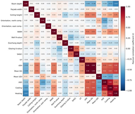
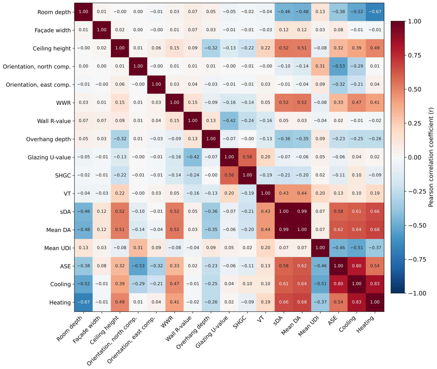
Before training the surrogate model, the statistical relationships among the design variables and performance indicators were examined using a Pearson correlation matrix (Figure 3). The matrix reflects the central architectural trade-off: the window-to-wall ratio (WWR) shows a moderate positive correlation with both annual cooling energy intensity (r = 0.47) and ASE (r = 0.33), indicating that larger glazing areas admit more daylight but also increase the thermal load and the potential for visual discomfort. Conversely, overhang depth is negatively correlated with cooling energy intensity (r = −0.25) and ASE (r = −0.23), confirming the role of shading in limiting solar gains.
Figure 3.
Pearson correlation matrix of the ten design variables and the six performance indicators (N = 1037). Orientation is represented by the north and east components of the window normal (the cosine and sine of the window azimuth). Room depth is the dimension perpendicular to the glazed façade, and façade width the dimension parallel to it.
Among the daylighting metrics, mean DA and sDA are almost perfectly correlated (r = 0.99), as both measure daylight sufficiency against the same 300 lux threshold. UDI behaves differently: it is essentially uncorrelated with DA and sDA (r = 0.07) and negatively correlated with ASE (r = −0.46) and cooling energy intensity (r = −0.51). This is expected, because UDI penalizes illuminance above its upper threshold of 3000 lux: designs that admit more direct sunlight raise DA and sDA but shift occupied hours into the exceeded range, thereby reducing UDI. The same behaviour appears in the building-scale cases (Section 4.3): the south-facing cases show higher mean DA (60.8–64.6%) but lower mean UDI (76.8–77.6%) than the north-facing cases (44.8–48.0% and 85.1–86.3%, respectively), because about 12.9% of their occupied hours exceed 3000 lux, compared with 3.4% for the north-facing cases.
Orientation is a circular variable whose effect is non-monotonic, so a single linear coefficient on the azimuth angle is not meaningful: its value depends on the arbitrary origin of the angle. In Figure 3, orientation is therefore represented by the north and east components of the window normal, which are moderately correlated with cooling energy intensity (r = −0.29 and −0.21) and with ASE (r = −0.53 and −0.32). In the full-factorial subset (Phase 1, 648 cases), where orientation takes eight discrete values, the mean cooling energy intensity ranges from 137.0 to 214.6 kWh/m2 across the orientations. In the same subset, the correlation ratio (η), which measures the dependence of a continuous output on a categorical input without assuming linearity, is 0.43 for cooling energy intensity and 0.74 for ASE, compared with linear coefficients on the azimuth angle of |r| = 0.17 and 0.45, respectively. Therefore, orientation influences performance strongly but non-linearly, a dependence that the Pearson coefficient cannot capture and that motivates the use of a non-linear model.
4.2. Surrogate Model Predictive Performance
Statistical evaluation metrics, including the coefficient of determination (R2), mean absolute error (MAE), root mean square error (RMSE), and mean absolute percentage error (MAPE), were used to analyze the predictive performance of the models in 10-fold cross-validation.
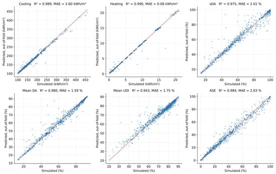
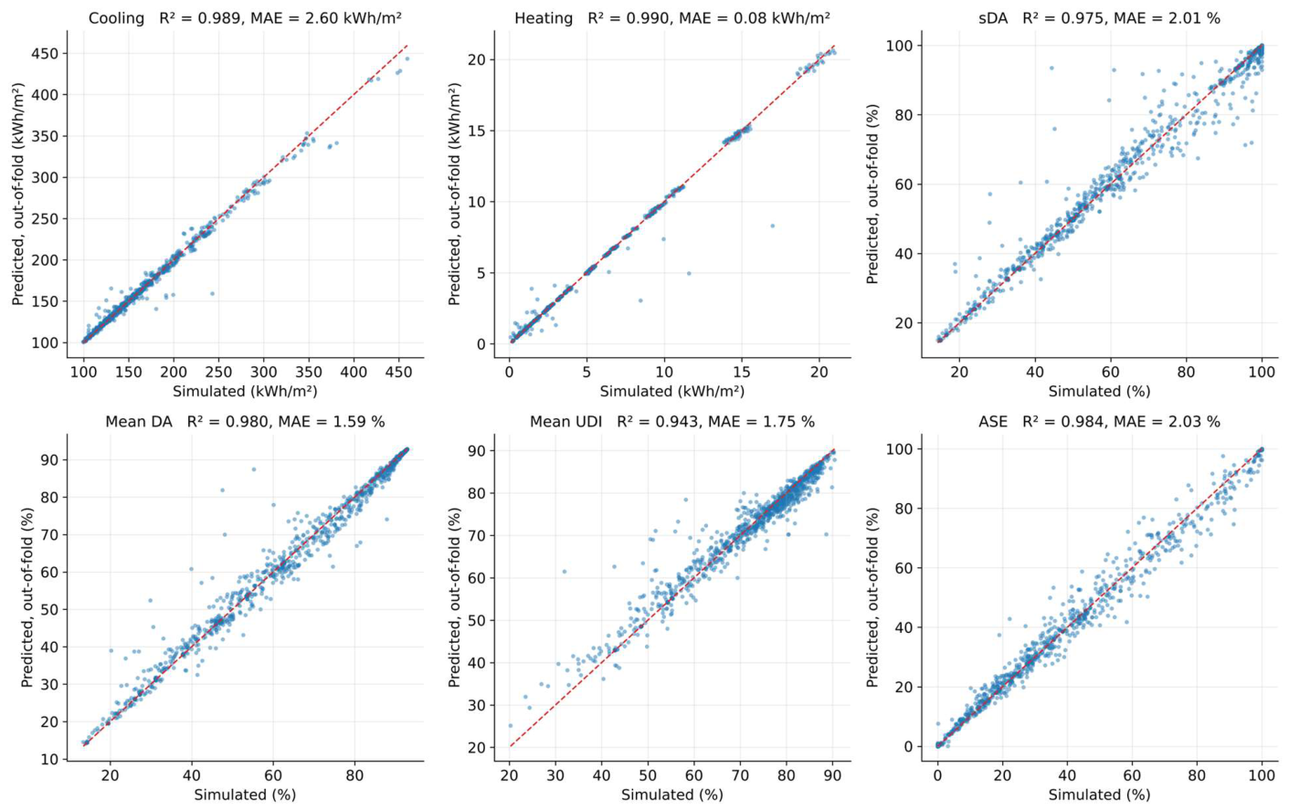
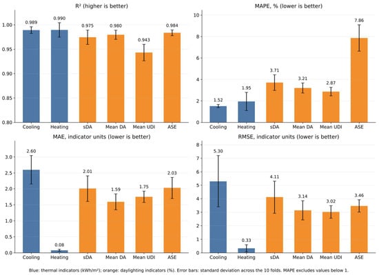
The cross-validation results are summarized in Table 2 and Figure 4. For annual cooling energy intensity, the surrogate achieved an R2 of 0.989 ± 0.007, an MAE of 2.60 kWh/m2, an RMSE of 5.30 kWh/m2, and an MAPE of 1.52%. For the daylighting indicators, the R2 ranged from 0.943 (mean UDI) to 0.984 (ASE), with MAEs between 1.59 and 2.03 percentage points.
Table 2.
Accuracy of the Random Forest surrogate models in 10-fold cross-validation (mean ± standard deviation over the folds; N = 1037). The MAPE excludes simulated values below 1.
Figure 4.
Out-of-fold predictions of the Random Forest surrogate models versus the simulation results for all 1037 cases (10-fold cross-validation) for the thermal (cooling, heating) and daylighting (sDA, mean DA, mean UDI, ASE) indicators. The dashed line indicates perfect agreement.
Across the six indicators, the R2 ranged from 0.943 to 0.990, and its fold-to-fold standard deviation did not exceed 0.017, indicating that accuracy is stable across different subsets of the data. As a reference for acceptable error, MAPE values below 10% are commonly classed as highly accurate predictions [30]; all indicators fell within this class, with MAPEs of 1.5–3.7%, except ASE (7.9%). For ASE, the MAPE is inflated by the many cases with values close to zero (north-facing or heavily shaded rooms), so its MAE of 2.0 percentage points is the more meaningful measure. The errors are also small relative to the differences that matter in design decisions: the sDA MAE of 2.0 percentage points is an order of magnitude smaller than the 20-point difference between the 55% and 75% sDA levels of IES LM-83-12, and the cooling MAE of 2.6 kWh/m2 is less than 2% of the median cooling intensity of the dataset (143 kWh/m2). For designs close to the 10% ASE limit, however, an error of 2 percentage points can change the outcome, and such designs should be confirmed by simulation. The surrogate is therefore suitable for early-stage design exploration, within the limits discussed in Section 4.5 (see Figure 5).
Figure 5.
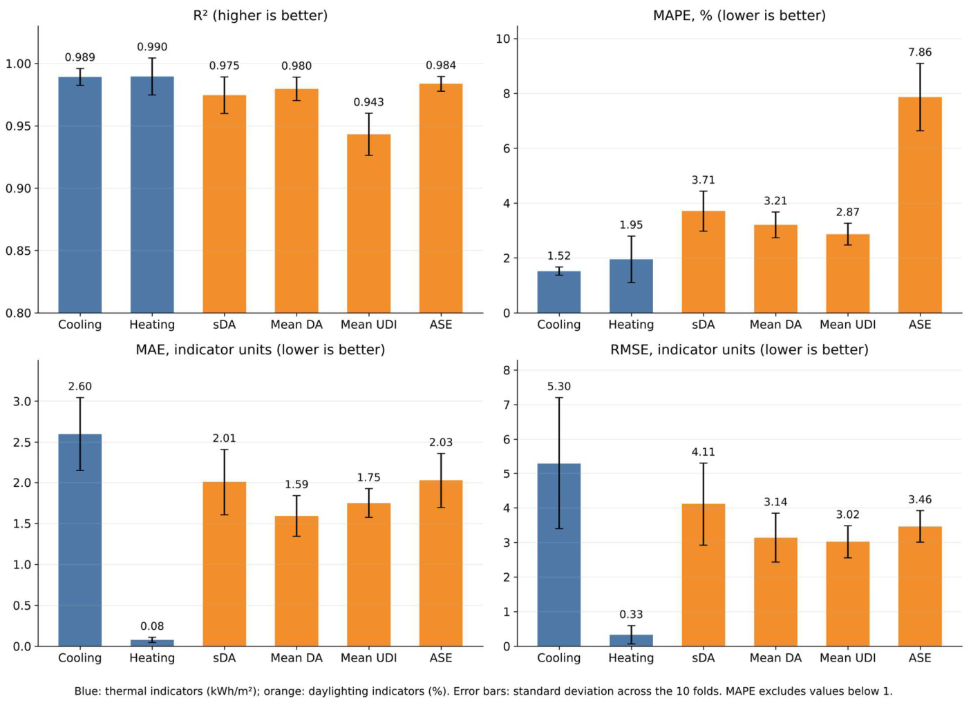
Accuracy metrics of the Random Forest surrogate models in 10-fold cross-validation (R2, MAPE, MAE and RMSE; error bars show the standard deviation over the folds) for the thermal (blue) and daylighting (orange) indicators.
The benchmark of the eight algorithms is reported in Appendix A (Table A1 and Table A2). The three tree-based ensembles and the MLP formed the most accurate group, with a mean R2 across the six indicators of 0.982 for Extra Trees and XGBoost, 0.977 for Random Forest, and 0.976 for MLP, followed by SVR (0.961) and Gradient Boosting (0.951). Multiple linear regression performed poorly (mean R2 = 0.710), confirming the strongly non-linear structure of the design space discussed in Section 4.1. Therefore, Random Forest was not the most accurate algorithm, but its deficit relative to the best algorithm was small, ranging from 0.002 (heating) to 0.023 (UDI) in R2; for four of the six indicators, this deficit was smaller than the fold-to-fold standard deviation of Random Forest itself. Random Forest was retained because these differences are small relative to cross-validation variability, because it is a robust and widely used algorithm for building-performance surrogates, and because the feature-importance analysis (Section 4.4) and the decision-support tool (Section 4.6) are built on it. Extra Trees and XGBoost are identified as marginally more accurate alternatives for future implementations.
4.3. Sensitivity of the Single-Zone Results to Building-Scale Position
To assess how far the adiabatic single-zone assumption limits the results, twelve additional simulations were carried out outside the training dataset. They represent a 6 × 6 × 3 m office room with a WWR of 0.4, no overhang, and the baseline envelope properties (Table 1), facing north or south. The room was located on the ground floor (floor in contact with the ground), on an intermediate floor (floor and ceiling adiabatic), or on the top floor (roof exposed to outdoor conditions), and in either a middle position (both side walls adiabatic) or a corner position (one side wall exposed, without glazing). Because floor level and plan position are not inputs of the surrogate model, these cases do not validate the surrogate; instead, they quantify the sensitivity of the simulated performance to conditions that the single-zone model excludes. The training dataset contains the corresponding single-zone case (Phase 2: same geometry, WWR, and envelope, no overhang, north- and south-facing), which allows a direct comparison of the daylighting results (Table 3).
Table 3.
Building-scale sensitivity cases (6 × 6 × 3 m room, WWR 0.4, no overhang) and the corresponding single-zone case from the training dataset (azimuth 270° for the north-facing and 90° for the south-facing window; see Table 1). Thermal results of the sensitivity cases are expressed relative to the intermediate-floor middle case, because these cases used the default Honeybee window construction.
Daylighting performance was almost insensitive to position. Across the twelve configurations, sDA differed from the corresponding single-zone case by −3.2 to +1.3 percentage points, the mean DA by −2.8 to +1.5 points, and the mean UDI by less than 0.7 points, while ASE was identical (0.44% for north and 33.11% for south). This is expected in an unobstructed context, where daylight enters only through the glazed façade, which is the same in all cases. The single-zone assumption is therefore adequate for the daylighting indicators.
Cooling energy intensity, by contrast, depended strongly on position. Because the twelve models used the default Honeybee window construction instead of the baseline glazing (U = 1.8 W/m2K, SHGC = 0.3), their absolute thermal results are not directly comparable with the training dataset. Thermal effects are therefore reported relative to the intermediate-floor middle room, whose boundary conditions match those of the single-zone model. Relative to this reference, cooling intensity decreased by up to 8.6% on the ground floor, where the floor exchanges heat with the ground, and increased by up to 18.5% on the top floor, where the roof is exposed; on the intermediate floor, the corner position added 3.0–5.3%. Heating intensity remained below 6 kWh/m2 in all cases but increased by 4.0–5.0 kWh/m2 on the top floor. The thermal predictions of the surrogate are therefore representative of rooms on intermediate floors in middle positions, whereas rooms under an exposed roof or at building corners can require substantially more cooling.
4.4. Feature Importance and Sensitivity Analysis
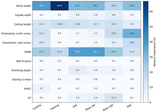
In an effort to improve upon the interpretability of the proposed model and deconvolute the “black box” nature within machine learning algorithms, a feature importance assessment was performed. Feature importance scores reflect the contribution and significance of each independent variable in determining the final predictions in tree-based ensemble algorithms such as Random Forest.
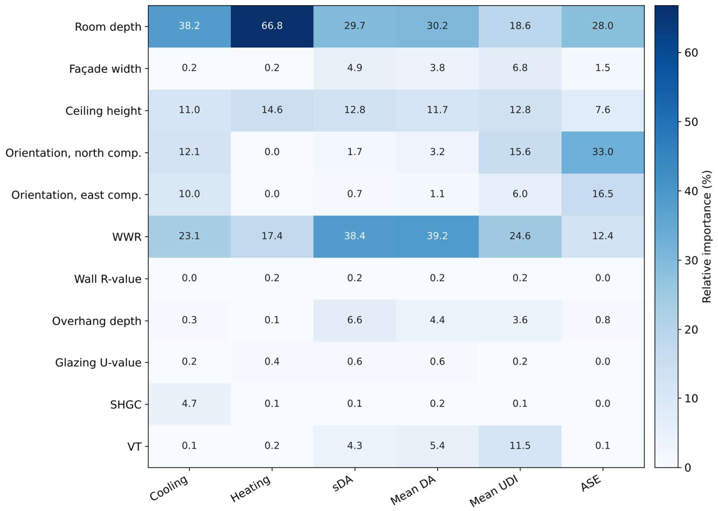
Figure 6 shows the relative importance of the design variables in the model of each indicator. Room depth, i.e., the distance from the glazed façade to the back wall, and the WWR were the most important variables for all indicators except ASE. Room depth dominated the thermal indicators (38% for cooling and 67% for heating) because it determines the floor area over which the façade heat gains are distributed, while the WWR dominated sDA and the mean DA (38–39%). Orientation, represented by its north and east components, contributed 22% for cooling and 50% for ASE, the indicator most directly governed by the sun path. Ceiling height contributed 8–15% to all indicators, and VT 4–12% to sDA, the mean DA, and the mean UDI. The envelope properties (wall R-value, glazing U-value, and SHGC) and the overhang depth were of minor importance in the dataset as a whole (below 7% for every indicator). This ranking must, however, be interpreted with the sampling design in mind: the envelope properties and the overhang were fixed in the 648 full-factorial cases; the overhang varied only in Phases 2 and 3, and the envelope properties only in Phase 3, so their importance is underestimated relative to a design space in which they vary freely. Within the 229 cases of Phase 3, in which they do vary, the SHGC accounted for 65% of the importance for cooling energy intensity and VT for 68% for sDA. The results nevertheless indicate that massing and window sizing should be prioritized at the early concept stage (see Figure 6).
Figure 6.
Relative importance (impurity-based, %) of the design variables in the Random Forest model of each performance indicator; the importances of each indicator sum to 100%. Orientation is represented by the north and east components of the window normal.
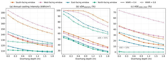
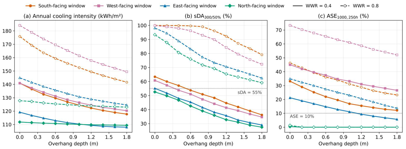
The Phase 2 cases (Section 3.2), in which only the overhang depth (0–1.8 m), the orientation, and the WWR were varied, show how overhang design depends on orientation (Figure 7). At a WWR of 0.4, a 1.8 m overhang (projection factor 0.95) reduced the cooling intensity by 16.4% for south-, 14.6% for west-, 9.4% for east-, and only 2.2% for north-facing windows, while sDA fell by 25–27 percentage points in every orientation. Overhangs on north façades therefore sacrifice daylight with almost no thermal benefit. The benefit also diminishes with depth: the first 0.6 m provided 42–56% of the cooling reduction obtained at 1.8 m. Finally, a horizontal overhang alone cannot control low-angle sun [11]. On west façades, ASE remained above 14% at every WWR even with a 1.8 m overhang, so west-facing and large south-facing windows require vertical fins or operable shading, which are outside the scope of this model.
Figure 7.
Effect of overhang depth on (a) cooling intensity, (b) sDA, and (c) ASE for the four window orientations (Phase 2 cases, 6 × 6 × 3 m room). Solid lines: WWR 0.4; dashed lines: WWR 0.8.
4.5. Multi-Objective Design Optimization and Pareto Front
Using the trained surrogate models, a multi-objective optimization (MOO) analysis was carried out to identify design configurations that reconcile two conflicting objectives: lower cooling energy intensity and higher sDA. The rapid predictions of the surrogate allow the design space to be screened at a small fraction of the cost of simulation-based optimization.
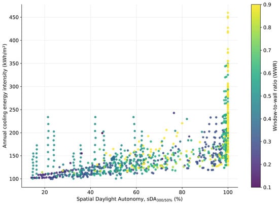
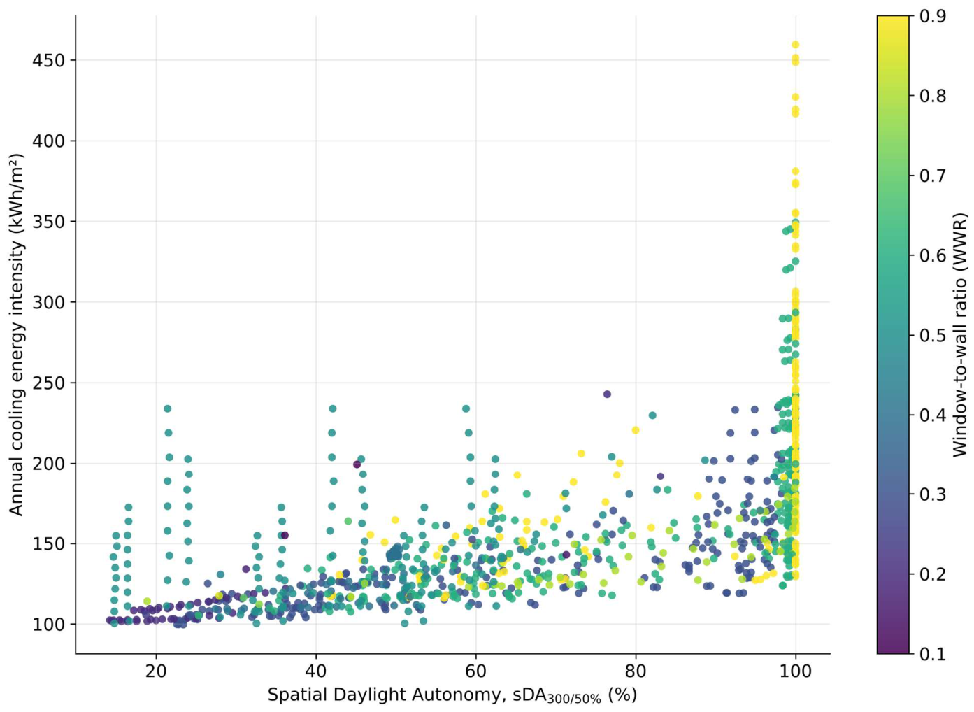
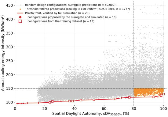
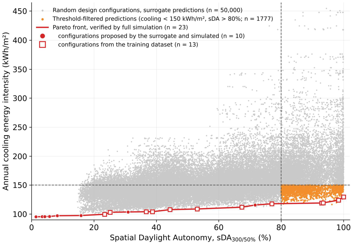
To illustrate the optimization, the simulated design space is first shown in Figure 8, which maps the trade-off between cooling energy intensity and sDA and the dominant influence of WWR. For the optimization, 50,000 design configurations were sampled uniformly at random within the variable ranges of Table 1, and their cooling energy intensity and sDA were predicted with the surrogate model. To exclude physically unrealizable glazing, the sampling was restricted to an SHGC of at least VT/2.2, i.e., a light-to-solar-gain ratio not exceeding 2.2, which is approximately the upper limit of commercially available spectrally selective glazing. A configuration is Pareto-optimal (non-dominated) when no other configuration has both a lower cooling energy intensity and a higher sDA. Configurations that satisfy two performance thresholds, a cooling energy intensity below 150 kWh/m2 and an sDA above 80%, are shown separately in orange (1777 configurations, of which only 4 are non-dominated).
Figure 8.
Simulated trade-off between annual cooling energy intensity and spatial Daylight Autonomy (sDA300/50%, static shading) for the 1037 design cases, colour-coded by the window-to-wall ratio (WWR).
The sDA threshold of 80% exceeds the 75% level that IES LM-83-12 regards as preferred daylight sufficiency; the additional margin reflects the fact that sDA computed with static shading is an upper bound of the LM-83 value (Section 3.1). The cooling threshold of 150 kWh/m2 lies close to the median cooling energy intensity of the simulated dataset (143 kWh/m2), so the filter retains designs that require less cooling than a typical configuration. Both thresholds are project-specific and can be adjusted in the dashboard.
Because the optimization deliberately seeks the extremes of the design space, where training data are sparse, the Pareto-optimal predictions were verified by full simulation. The non-dominated configurations predicted by the surrogate were simulated with the same Honeybee model definition, added to the training data, and the surrogate was refitted; this adaptive infill was repeated for eight rounds (124 simulations). The infill simulations were run through the Ladybug Tools Python SDK (honeybee-energy and honeybee-radiance, EnergyPlus 24.2, Radiance 5.4a) instead of Grasshopper; for 12 randomly selected cases of the training dataset, this workflow reproduced the Grasshopper results with a mean absolute percentage error of 0.4% for cooling energy intensity and a mean absolute error of 1.1 percentage points for sDA, with identical ASE values.
Before being simulated, the configurations proposed by the surrogate were predicted with a mean absolute percentage error of 4.8% for cooling energy intensity and a mean absolute error of 15.8 percentage points for sDA (median 11.7), decreasing to 4.0% and 7.8 points in the last round. The surrogate overestimated sDA for these configurations by 12.7 points on average. These errors are much larger than the cross-validated errors of Section 4.2 because the optimizer selects precisely those configurations whose daylight performance the surrogate overestimates. The Pareto front in Figure 9 is therefore drawn exclusively from simulated configurations that satisfy the glazing constraint (23 configurations: 13 from the training dataset and 10 found by the surrogate-guided search). Along this front, cooling energy intensity rises from 95 to 112 kWh/m2 as sDA increases to 67%, remains at 118–119 kWh/m2 between an sDA of 77% and 93%, and reaches 124–129 kWh/m2 for an sDA of 98–100%. The front configurations with an sDA of 75% or more face north or north-east, and all but one use the baseline glazing (SHGC 0.30, VT 0.64). The surrogate-guided search found no configuration that outperformed the simulated dataset for an sDA between 55% and 95%, and lowered the cooling energy intensity required for an sDA of 99% or more by only 1.3%. The surrogate is therefore best used for rapid screening of the design space, with final candidates confirmed by simulation.
Figure 9.
Multi-objective optimization. Grey: 50,000 random design configurations with physically realizable glazing (SHGC ≥ VT/2.2) predicted by the surrogate model; orange: predictions meeting the performance thresholds (cooling energy intensity < 150 kWh/m2, sDA > 80%); red line: Pareto front verified by full simulation, comprising configurations proposed by the surrogate and subsequently simulated (circles) and configurations from the training dataset (squares).
4.6. Computational Efficiency and Design Optimization
The main motivation for the creation of this machine learning surrogate model is to alleviate the severe computational bottlenecks that traditional building performance simulation (BPS) methods incur. A single physics-based simulation run through Grasshopper and Honeybee for the generation of thermal and daylighting metrics took, on average, 55 s. Consequently, it would be very difficult to go through thousands of design iterations with traditional tools in the early stages of design.
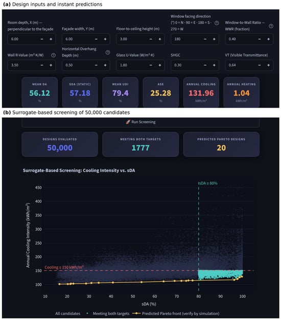
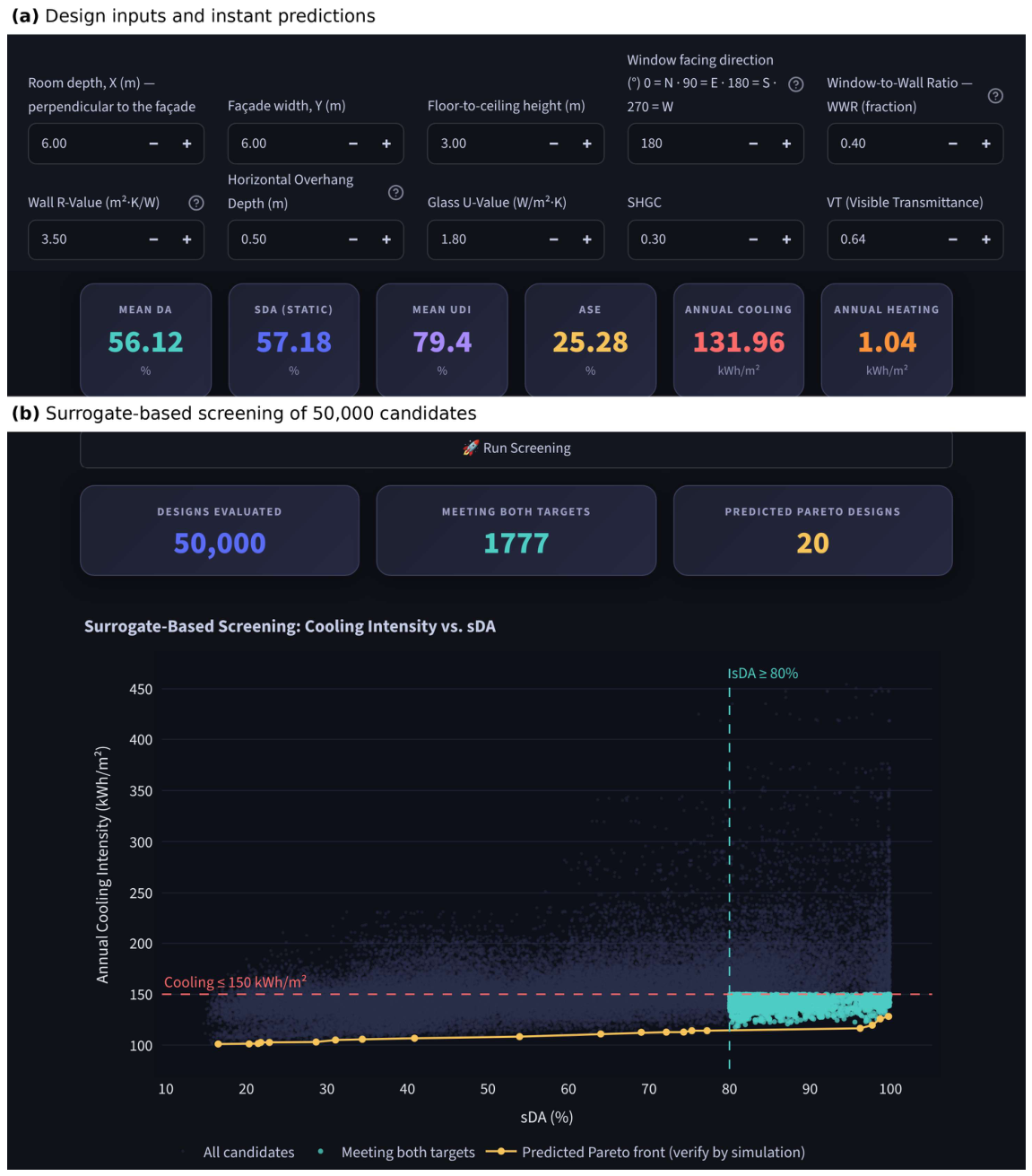
Conversely, the Random Forest surrogate models developed in this work, incorporated into the interactive tool presented here (Figure 10), predict all six indicators for a design configuration in about 0.3 s on a standard computer and evaluate 50,000 configurations in about 12 s. This rapid feedback allows architects to screen a large design space quickly and to identify promising configurations, which should then be confirmed by simulation (Section 4.5).
Figure 10.
The interactive decision-support tool: (a) design inputs and instant predictions of the six indicators, and (b) screening of 50,000 random candidates with realizable glazing against user-defined targets (here, cooling ≤ 150 kWh/m2 and sDA ≥ 80%), with the predicted Pareto front, whose designs should be confirmed by simulation.
5. Conclusions
This study presents a fast parametric framework combining building performance simulation (BPS) and machine learning to explore the conflicting relationship between cooling energy intensity (kWh/m2) and spatial Daylight Autonomy (sDA) in early-stage office design. By focusing specifically on the hot arid climate of Cairo, Egypt, a large dataset of 1037 design scenarios—regular, slanted, and extreme—was generated to assess initial exploration of the design space.
In 10-fold cross-validation, the Random Forest surrogate models reproduced the simulation outputs with an R2 of 0.943–0.990 and an MAPE below 4% for all indicators except ASE (7.9%), and a benchmark of eight algorithms showed that their accuracy was within 0.023 in the R2 of the most accurate algorithm for every indicator. The surrogate reduces the evaluation time of a design configuration from about 55 s to about 0.3 s.
The feature importance analysis identified room depth and the window-to-wall ratio as the most influential variables overall and orientation as the dominant variable for sunlight exposure, although the influence of the envelope properties is underestimated by the sampling design, in which they vary only in part of the dataset. A surrogate-assisted multi-objective optimization was performed, and the Pareto-optimal designs were verified by full simulation. The verification showed that the surrogate overestimates daylight performance at the extremes of the design space, and the verified front shows that north- and north-east-facing rooms with the baseline glazing achieve an sDA above 90% at a cooling energy intensity of about 119 kWh/m2.
In addition, twelve building-scale simulations showed that the single-zone assumption is adequate for the daylighting indicators (sDA within 3.2 percentage points of the corresponding single-zone case), but that a room under an exposed roof can require up to 18.5% more cooling than an intermediate-floor room. The surrogate’s thermal predictions should therefore be read as representative of intermediate-floor rooms.
This research delivers a rapid decision-support tool that enables architects and practitioners to screen thousands of design alternatives (see Figure 10), with promising candidates confirmed by simulation.
Although the surrogate model closely reproduces the simulation outputs, its applicability is bounded by the assumptions of its training data. It is intended for early conceptual massing and façade decisions. It represents a single-zone office room with adiabatic interior surfaces, an unobstructed site, and fixed horizontal overhangs, and its accuracy refers to agreement with a simulation model that was not calibrated against measured data. Detailed design stages therefore still require multi-zone thermal and airflow simulation, the shading of the actual urban context [24], and operable shading, which Section 4.4 shows to be necessary for west-facing and large south-facing windows. The results also apply to the hot arid climate of Cairo only. Future studies should extend the framework to other building types, climates, urban contexts, and shading systems, and to further objectives such as life cycle cost (LCC) and carbon emissions [4,21].
Funding
This research received no external funding.
Institutional Review Board Statement
Not applicable.
Informed Consent Statement
Not applicable.
Data Availability Statement
The data that support the findings of this study are available from the corresponding author upon reasonable request.
Acknowledgments
AI Use Declaration During the preparation of this work, the author utilized generative AI tools, specifically Gemini 3.1 Flash and Claude Sonnet 4.6. Gemini 3.1 Flash was used primarily to improve readability and the overall English phrasing of the manuscript. Furthermore, Claude was employed to assist in editing and debugging the underlying scripts used in the simulation methodology. During revision, Claude Opus 5.5 (Anthropic) was used to assist in writing and running the Python scripts for the cross-validation. After using these tools, the author thoroughly reviewed, validated, and edited the generated content and code as needed, and takes full responsibility for the final content, originality, and integrity of the publication.
Conflicts of Interest
The author declares no conflicts of interest. He has no known competing financial interests or personal relationships that could have appeared to influence the work reported in this paper.
Appendix A. Benchmark of Regression Algorithms
Table A1.
Coefficient of determination (R2, mean ± standard deviation over 10 folds) of eight regression algorithms for the six performance indicators (N = 1037; default library hyperparameters, except 1000 trees for Random Forest, as in the surrogate model).
Table A2.
The mean absolute error (MAE) and, in parentheses, the root mean square error (RMSE), reported as MAE (RMSE), both averaged over 10 folds, of the eight algorithms. Units: kWh/m2 for cooling and heating; percentage points for the daylighting indicators.
Appendix B. Grasshopper Definition
Figure A1.
The parametric visual scripting workflow developed in Grasshopper, integrating Honeybee and Ladybug plugins for automated building geometry generation, material assignment, and data-driven batch simulation.
References
- Ali, A.; Jayaraman, R.; Mayyas, A.; Alaifan, B.; Azar, E. Machine learning as a surrogate to building performance simulation: Predicting energy consumption under different operational settings. Energy Build. 2023, 286, 112940. [Google Scholar] [CrossRef] [Scilit]
- Elkabalawy, M.; Al-Sakkaf, A.; Mohammed Abdelkader, E.; Alfalah, G. CRISP-DM-Based data-driven approach for building energy prediction utilizing indoor and environmental factors. Sustainability 2024, 16, 7249. [Google Scholar] [CrossRef] [Scilit]
- Westermann, P.; Evins, R. Surrogate modelling for sustainable building design—A review. Energy Build. 2019, 198, 170–186. [Google Scholar] [CrossRef] [Scilit]
- Elwy, I.; Hagishima, A. The artificial intelligence reformation of sustainable building design approach: A systematic review on building design optimization methods using surrogate models. Energy Build. 2024, 323, 114769. [Google Scholar] [CrossRef] [Scilit]
- Markarian, E.; Qiblawi, S.; Krishnan, S.; Divakaran, A.; Ramalingam Rethnam, O.; Thomas, A.; Azar, E. Informing building retrofits at low computational costs: A multi-objective optimisation using machine learning surrogates of building performance simulation models. J. Build. Perform. Simul. 2024, 19, 894–910. [Google Scholar] [CrossRef] [Scilit]
- Li, X.; Yuan, Y.; Liu, G.; Han, Z.; Stouffs, R. A predictive model for daylight performance based on multimodal generative adversarial networks at the early design stage. Energy Build. 2024, 305, 113876. [Google Scholar] [CrossRef] [Scilit]
- Stevanović, S.; Dashti, H.; Milošević, M.; Al-Yakoob, S.; Stevanović, D. Comparison of ANN and XGBoost surrogate models trained on small numbers of building energy simulations. PLoS ONE 2024, 19, e0312573. [Google Scholar] [CrossRef] [Scilit] [PubMed]
- Wu, Z.; Li, M.; Liu, W.; Cheng, J.C.P.; Wang, Z.; Kwok, H.H.L.; Huang, C.; Hou, F. Developing surrogate models for the early-stage design of residential blocks using graph neural networks. Build. Simul. 2025, 18, 679–698. [Google Scholar] [CrossRef] [Scilit]
- Shen, Y.; Pan, Y. BIM-supported automatic energy performance analysis for green building design using explainable machine learning and multi-objective optimization. Appl. Energy 2023, 333, 120575. [Google Scholar] [CrossRef] [Scilit]
- Alsharif, R.; Arashpour, M.; Golafshani, E.; Rashidi, A.; Li, H. Multi-objective optimization of shading devices using ensemble machine learning and orthogonal design of experiments. Energy Build. 2023, 283, 112840. [Google Scholar] [CrossRef] [Scilit]
- Kirimtat, A.; Koyunbaba, B.K.; Chatzikonstantinou, I.; Sariyildiz, S. Review of simulation modeling for shading devices in buildings. Renew. Sustain. Energy Rev. 2016, 53, 23–49. [Google Scholar] [CrossRef] [Scilit]
- Hou, D.; Evins, R. A protocol for developing and evaluating neural network-based surrogate models and its application to building energy prediction. Renew. Sustain. Energy Rev. 2024, 193, 114283. [Google Scholar] [CrossRef] [Scilit]
- Zorn, M.; Claus, L.; Frenzel, C.; Wortmann, T. Optimizing an expensive multi-objective building performance problem: Benchmarking model-based optimization algorithms against metaheuristics with and without surrogates. Energy Build. 2025, 336, 115562. [Google Scholar] [CrossRef] [Scilit]
- Shirzadi, N.; Lau, D.; Stylianou, M. Surrogate modeling for building design: Energy and cost prediction compared to simulation-based methods. Buildings 2025, 15, 2361. [Google Scholar] [CrossRef] [Scilit]
- Zhou, F.; Yang, C.; Wang, Z. Prediction of building energy consumption for public structures utilizing BIM-DB and RF-LSTM. Energy Rep. 2024, 12, 4631–4640. [Google Scholar] [CrossRef] [Scilit]
- Golafshani, E.; Chiniforush, A.A.; Zandifaez, P.; Ngo, T. An artificial intelligence framework for predicting operational energy consumption in office buildings. Energy Build. 2024, 317, 114409. [Google Scholar] [CrossRef] [Scilit]
- Xu, W.; Tu, J.; Xu, N.; Liu, Z. Predicting daily heating energy consumption in residential buildings through integration of random forest. Energy 2024, 301, 131726. [Google Scholar] [CrossRef] [Scilit]
- Elhabyb, K.; Baina, A.; Bellafkih, M.; Deifalla, A.F. Machine learning algorithms for predicting energy consumption in educational buildings. Int. J. Energy Res. 2024, 2024, 6812425. [Google Scholar] [CrossRef] [Scilit]
- Boutahri, Y.; Tilioua, A. Machine learning-based predictive model for thermal comfort and energy optimization in smart buildings. Results Eng. 2024, 22, 102148. [Google Scholar] [CrossRef] [Scilit]
- Álvarez-Sanz, M.; Satriya, F.A.; Terés-Zubiaga, J.; Campos-Celador, Á.; Bermejo, U. Ranking building design and operation parameters for residential heating demand forecasting with machine learning. J. Build. Eng. 2024, 86, 108817. [Google Scholar] [CrossRef] [Scilit]
- Hosamo, H.; Coelho, G.B.A.; Rolfsen, C.N.; Kraniotis, D. Building performance optimization through sensitivity analysis, and economic insights using AI. Energy Build. 2024, 325, 114999. [Google Scholar] [CrossRef] [Scilit]
- Araújo, G.R.; Gomes, R.; Ferrão, P.; Gomes, M.G. Optimizing building retrofit through data analytics: A study of multi-objective optimization and surrogate models derived from energy performance certificates. Energy Built Environ. 2024, 5, 889–899. [Google Scholar] [CrossRef] [Scilit]
- Lédée, F.; Crawford, C.; Evins, R. Improved surrogate modeling for multi-energy system design: Model architecture, sampling and scaling choices. Appl. Energy 2025, 390, 125812. [Google Scholar] [CrossRef] [Scilit]
- Yoo, W.; Kim, H. A surrogate modeling approach for evaluating the shading effect on building energy performance. Dev. Built Environ. 2025, 24, 100796. [Google Scholar] [CrossRef] [Scilit]
- Reinhart, C.F.; Mardaljevic, J.; Rogers, Z. Dynamic daylight performance metrics for sustainable building design. Leukos 2006, 3, 7–31. [Google Scholar] [CrossRef] [Scilit]
- Nabil, A.; Mardaljevic, J. Useful daylight illuminances: A replacement for daylight factors. Energy Build. 2006, 38, 905–913. [Google Scholar] [CrossRef] [Scilit]
- IES LM-83-12; IES Spatial Daylight Autonomy (sDA) and Annual Sunlight Exposure (ASE). Illuminating Engineering Society of North America: New York, NY, USA, 2012.
- Roudsari, M.S.; Pak, M. Ladybug: A parametric environmental plugin for Grasshopper to help designers create an environmentally-conscious design. In Proceedings of the 13th International Conference of the International Building Performance Simulation Association, Chambéry, France, 26–28 August 2013; pp. 3128–3135. [Google Scholar]
- Loeppky, J.L.; Sacks, J.; Welch, W.J. Choosing the sample size of a computer experiment: A practical guide. Technometrics 2009, 51, 366–376. [Google Scholar] [CrossRef] [Scilit]
- Lewis, C.D. Industrial and Business Forecasting Methods: A Practical Guide to Exponential Smoothing and Curve Fitting; Butterworth Scientific: London, UK, 1982. [Google Scholar]

Disclaimer/Publisher’s Note: The statements, opinions and data contained in all publications are solely those of the individual author(s) and contributor(s) and not of MDPI and/or the editor(s). MDPI and/or the editor(s) disclaim responsibility for any injury to people or property resulting from any ideas, methods, instructions or products referred to in the content. |
© 2026 by the author. Licensee MDPI, Basel, Switzerland. This article is an open access article distributed under the terms and conditions of the Creative Commons Attribution (CC BY) license.