


Abstract
The increased interest in environmental sustainability, driven by the transition to renewable energies, has spotlighted woodchip as an effective alternative to fossil fuel. Despite being readily available, its natural origin results in inherent heterogeneity, affecting every stage of the supply chain up to the combustion. Firstly, moisture content is detrimental for calorific value, leading to ineffective combustion drawbacks in transport and challenging storage. Water content monitoring along the production chain is crucial but its evaluation with standard analyses is limited due to destructive approach, unsuitable schedules and consequent costs. Near-infrared spectroscopy (NIRS), as an alternative technique, provides a non-destructive, repeatable, and faster method for both lab and inline control, overcoming standards limits. Considering the comparation already run with equal method, NIRS performances in predicting moisture content in Italian industrial woodchip simulating an in-line system are evaluated. Steady collection of continuous replicates improves woodchip representativeness, reducing estimation bias and enhancing prediction reliability (determination coefficient ~0.9, error <3%). Given the qualitative screening results, NIRS shows high water detection ability, acting as portable tool for real-time characterization in power plants. The immediate evaluation of water content could support critical steps along the supply chain, contributing to clean energy and market safety.
1. Introduction
The increasing utilization of renewable energy resources (RESs), with the consequent reduction in fossil fuel consumption, represents a key objective of European energy policies. This unavoidable transition, driven both by the depletion of non-renewable fossil fuels and by the current socio-political and economic challenges, aligns with the climate neutrality target disposed by the European Green Deal until 2050, through the adoption of green transition, a low-carbon economy, and the net reduction of greenhouse-gas (GHG) emissions [1,2]. The EU Directive 2018/2001 established the minimum threshold of 32% of energy from RESs in gross energy consumption by 2030, later increased to 40% in 2021. Moreover, the “Fit for 55” package outlines several initiatives to support the energy transition, promote a diversified energy supply, and address climate vulnerability and biodiversity protection [3]. In this context, forests play a crucial role, as recognized by the EU Forest policy, which contributes to a climate-neutral and sustainable economy through ecosystem services and the carbon-saving potential of forest products, enhancing resilience, biodiversity, and multifunctionality [4]. However, continuous deforestation (approximately 4.7 million hectares per year) [4], but also the COVID-19 pandemic situation, and the recent geopolitical conflicts in Ukraine and Gaza, have exposed the fragilities of EU’s economic and energy systems, and have highlighted the urgent need to strengthen energy independence. Consequently, the EU needs to take actions resulting in the boost of its RES target from 40 to 45% in total [2]. Therefore, these historical events are accelerating the phase-out of non-reliable energy sources and fostering the deployment of secure, sustainable, and competitive alternatives [3].
Among the available bioenergy sources, solid biomass represents a valid contribution, supported by the extensive forest coverage in the EU (43.5% of the European total land area) and by the 20% increase in wood-based energy since 2000, accounting for about 60% of the renewable energy consumption [4]. In 2019, 23% of roundwood in Europe (60% in Italy) was used for energy production, although there was a slight decrease in 2020 due to the socio-political and economic disruptions [1]. In particular, RES employment reached 105 Mtoe in the electricity sector, and 87 Mtoe for thermal generation, with bioenergy as the largest contribution [5]. The same trend is confirmed in Italy, where electricity generation from solid biomass increased from 5.1% in 2012 to 5.8% in 2020, despite the production of electricity from RESs attaining 38% in 2020; while 20% of RESs are used to produce thermal energy, where about 60% of the total came from solid biomass for residential use, confirming the key role of woody fuels, such as firewood and pellets [5,6,7].
Therefore, to ensure an efficient and sustainable use of biomass, a cascade approach became essential to correctly allocate woody biomass according to its highest economic and environmental value in line with the waste hierarchy principles. This approach supports the promotion of bioenergy, the preservation of national carbon sinks, and the development of innovative solutions to valorize uncompetitive renewable resources [2]. Moreover, the simplification of the authorization procedures and the integration of innovative control methods could effectively strengthen the confidence in supporting RES markets, enhancing accessibility, circular economy practices, and common growth [3].
Among solid biomass, woodchip is recognized as a versatile and cost-effective feedstock that benefits from the implementation of innovative monitoring systems to continuously manage its inherent heterogeneity. Thanks to its natural and renewable origin, minimal processing requirements, and carbon neutrality strength, industrial woodchip is widely considered a worthwhile resource, as a valuable provider of ecosystemic services and for energy production [8,9]. Despite larger advantages, quality characterization becomes a crucial process, because of its diversified composition related to origin, season and climate influence during its handling, including harvesting, transport, and storage [10,11]. The simultaneous presence of broadleaf and conifer logging residues, offcuts, small trees, dedicated timber and short rotation coppice, as well as sawmill residues, as long as virgin, pruning with tops and branches, but also sawdust, leaves, needles, bark, and stock leftover, affect the energy conversion process and supply chain efficiency [12], frequently making visual recognition of each component challenging [10].
Moisture content (MC), above all the physical and chemical parameters influenced by composition, affects the combustion process, resulting in reduced energy conversion and higher pollutant emissions such as carbon monoxide [13,14]. High MC also means the useless transport of a useless amount of water instead of biomass, causing the additional loss of material due to the proliferation of microbiological populations, as well as self-ignition events caused by the occurrence of adverse internal and external conditions during storage [15,16]. As a result, MC significantly influences logistic operations, affecting timelines of the drying process, and consequently decreasing the economic value of the biomass, as well as the profitability scale along the entire supply chain [16]. The accurate determination of MC in woodchip remains a tough challenge, due to its extreme variability across forestry species, season oscillations, and climatic conditions, which is reflected in handling, transport, and storage practices [16,17,18]. MC monitoring became a fundamental step to drive the best operative execution of the combustion process and to guarantee a suitable utilization of each feedstock, according to ISO 17225 statements [12], minimizing technical problems and environmental detriments related to uncontrolled quality definition [14].
Although standard ISO 18134-2 [19] provides the reference method for MC measurement, it remains a single-sample and destructive approach that lacks replicability and reproducibility thresholds, leading to neither representative nor objective results [14] and precluding replicate collection. Besides, the standard method execution is time-consuming (up to 24 h of standby) and demanding in terms of hourly costs, laboratory equipment, and skilled personnel requirements [20,21], limiting its practical applicability outside of a staged lab [22]. Despite the standard method enabling the execution of common procedures in laboratories, the implementation of non-destructive and effortless methods has become essential to face the limits of standards and to guarantee reliable results in more favorable conditions.
Among these, near-infrared spectroscopy (NIRS) is widely considered a promising technique providing a non-destructive and faster approach, with minimal or no sample preparation and reduced operational costs related to lab experience [23,24]. In fact, the easy and intuitive NIRS employment improves in-field, on-line, and at-line implementation in industrial contexts, facilitating the acquisition of several replicates and the following representative scenario for determining the main chemical and physical features. So, the possibility to acquire an unlimited number of scans, covering the entire layer of the investigated material, could overcome the lack of reproducibility of the standard ISO, providing a complete examination. Thus, NIRS permits the proper estimation of many qualitative and quantitative properties by correlating the spectral absorbance data with the chemical composition [25]. Through the chemometrics computing and multivariate data analysis, the extraction of useful information from spectral data represents a key step that requires the fundamental assistance of expertise, resulting in the development of reliable classification and prediction models [23]. NIRS effectively detects water bonds (O-H) and single bonds such as C-H, N-H, and S-H [23,25], although overtone and combination bands and temperature variations can influence the spectral interpretation [24,26]. Calibration is therefore a basic step to achieve accurate and reproducible prediction practically suitable in the operative process [27].
MC is accurately detected in the NIR range (780–2500 nm) [28], so the application of portable or miniaturized NIR spectrometers, widely distributed, enables real-time and in-field MC estimation along the most critical stages of the biomass supply chain, including direct application in power plants, to enhance comprehensive monitoring and the choice of the most suitable settings during combustion [29]. Several studies have confirmed the capability of NIRS to predict MC in woodchips [22,30,31], in different energy crops [32], but also in alternative biomass sources [27,33,34], including woody pellets [35]. Nonetheless, only a few studies have investigated NIRS performance under dynamic or in-line conditions. For instance, models developed with a non-contact procedure—where a minimum distance between sample and detector is maintained—have yielded accurate MC predictions while improving a more complete representativeness [34]. Furthermore, on-line monitoring along conveyor belts, as in the pulp and paper industry, could enhance process control and reduce variability challenges associated with natural biomass [35]. However, practical applications remain limited, providing a small dataset, and further validation will be decisive to strengthen confidence in the implementation of NIRS monitoring systems.
Based on the application of two portable NIR spectrophotometers and the gathering of a larger dataset, this study proposed the comparison of their practical and technical performances in predicting the MC of industrial woodchips under simulated in-line conditions using a rotating plate. Assuming their potential implementation along conveyor belts directly in power plants, the achievements of the investigation already performed with the Polispec NIR portable spectrophotometer [36] have been matched with the novel employment of the MicroNIR spectrophotometer, tested under an equal circular motion of the same rotating plate, thanks to its ergonomic design and its intuitive use. Therefore, multiple replicate spectra have been collected, allowing the development of three PLS prediction models for the MC parameter. To present a comprehensive evaluation, the performance of the MicroNIR has been compared with the previous results from the PolispecNIR [36] in terms of: (i) raw spectra profiles, (ii) prediction models development, (iii) prediction statistics and the distribution of samples according to MC classes, (iv) bias margins using Prediction Range Definition (PRD), and (v) outliers detection via Tukey’s Test (TT).
2. Materials and Methods
2.1. Collection of Woodchip Samples and Database Assessment
For each analysis method applied (means as the analysis approach and expressed as MET), a specific number of industrial woodchip samples were collected from several Italian power plants and analyzed (Table 1). The material used for D-PIL and D-MIL originated from the same power plants.
Table 1.
Brief scheme showing the essential information of each analysis method (MET) applied for the analysis of the moisture content of woodchip samples.
The two datasets have a similar number of samples (103 vs. 99) and of replicates (assuming that the number of replicates in MET2 is equal to 3 for each dataset). The divergent number of MET3 D-PIL is related to the peculiarity of its acquisition mode and, in particular, to the spectrophotometer setting. In detail: by default, D-PIL collects a casual number of scans, leading to one averaged spectrum-scan. During the swipe, around 46 swipe-scans for each of the 3 replicates (then averaged according to MET1 and MET2) were collected, that means between 118 and 145 for each sample. D-MIL collects 1000 internal scans that are automatically averaged by its software (MicroNIR PRO Software, ver.3.0), leading to one spectrum-scan. Then, during the swipe, 3 swipe-scans were collected for each of the 3 replicates, resulting in 9 swipe-scans for each sample (99 × 3 × 3 = 891). As recommended by the technical standard EN ISO 18135:2017—Sampling of solid biofuels [37], about 2 kg for each woodchip sample was delivered to the lab, hermetically locked in single plastic bags to preserve the same physical and chemical properties of the sampling moment. Therefore, each sample can be considered representative of the corresponding woodchip piles of origin, which come from several tons of different particle size, fine content, impurities, and tree portions [14]. Thus, each biomass sample can feature a wide range of quality characteristics, which provides a comprehensive description of Italian commercialized woody fuel and its inherent heterogeneity. In fact, samples consist of forest residues (broadleaves as well as conifers), but also of dedicated energy crops (e.g., poplar short rotation coppice), agricultural residuals (mainly from orchards), but also residues from riverbanks maintenance (a mix of broadleaves). As a result, complete information about the specific origin of each sample was not noted by the power plants, despite the material being able to be considered representative of the national flux of industrial woodchip, as confirmed in the specific monitoring of the same biofuel typology [13]. Moreover, the different collection periods did not lead to significant discrepancy also in terms of water content. In fact, the measured MC values of both datasets were investigated with a Q-Q plot test, confirming the normal distribution of data for both collection sets. In addition, the third quartile (Q3) value of D-PIL matched well with the analogous value of D-MIL (45.65% and 43.04%, respectively), as did the interquartile range (IQR) of D-PIL compared with the result for D-MIL (10.10 and 10.07, respectively). As confirmed, a two-sample t-test was developed, resulting in a p-value higher than 0.05 as the critical value; this score permits the acceptance of the null hypothesis and to conclude that no significant difference between the two datasets can be registered, allowing their comparation.
2.2. Moisture Content Analysis
Considering its aforementioned relevance in the energy definition, moisture content (MC) has been considered the benchmark for the qualitative assessment of biofuel, and it is measured according to the standard methodology established by ISO 18134:2015—Determination of moisture content [19]. Assuming the occurrence of physical modification during analysis and the single-measurement method, representative analysis must be ensured with the collection of reliable data; so, each sample, analyzed individually, was firstly mixed and then homogeneously distributed on a non-corrodible and heat-resistant tray, previously weighed as tare. The weight of the prepared sample, carefully shred in a volume of 30 × 24 × 5 cm to fulfil a minimum mass of biomass of 300 gr, was recorded before placing it in ventilated oven under controlled temperature (105 ± 2 °C) for a maximum of 24 h until it reached constant weight. Moreover, samples were placed in each oven slot to avoid overloading and to ensure adequate free air flow between them, favoring the correct drying process, considering that the relevant degree of heterogeneity, due to the presence of different species and different parts of biomass (chips from branches and trunk, but also undesirable parts like bark, needles, etc.), could negatively influence the completion of the drying time.
2.3. Near-Infrared Spectroscopy and Spectral Collection
Two different portable NIR spectrophotometers were employed, while a specific analysis method was applied simulating in-line application in the laboratory, with the aim of comparing their performance. In detail, these were the PolispecNIR instrument (distributed by ITPhotonics S.r.l., Fara Vicentino, Italy), abbreviated as Polispec, and the MicroNIR OnSite instrument (Viavi Solutions Inc., Santa Rosa, CA, USA), abbreviated as Micro. The Polispec works in the range 900–1700 nm, and the acquisition is carried out in reflectance, while an internal reference measurement is acquired during the analysis. The integration time is set at 10 ms, so each spectrum is the average of several scans collected over around 5 s. It is equipped with one halogen lamp as radiation source and a 256-pixel indium gallium arsenide (InGaAs) photodiode array as detector. The heat dissipator, placed in the frontal part and combined with the cooling control system, permits it to avoid signal deformation due to temperature variation, for example due to external conditions. Despite its weight (about 3 kg), it is used as a portable instrument thanks to its compact and durable case of anodized aluminum, supported by a handle on the top of the case. Furthermore, its large optic area (3.2 cm2), designed to be suitable for motion fluxes, but also the internal power source and the available remote control through Bluetooth connection, supports manual, user-friendly, and in-field applications.
In contrast, the Micro works in the range 950–1650 nm, while the acquisition is carried out in reflectance, with the integration time of 6.7 ms, so each spectrum is the automatic average of different scans. A reference standard (Spectralon) is acquired every hour or when external conditions change, with the aim to remove the instrument as well as the environment noise, thanks to the collection of a dark reference (0% transmittance) and a blank spectrum (99% reflectance). Instead of Polispec, two internal vacuum tungsten lamps act as radiation source, with Linear Variable Filter coupled with a 128-pixel indium gallium arsenide (InGaAs) photodiode array as detector. Moreover, the ergonomic, light (about 200 gr of weight) and handy case of the Micro, easily maneuverable like a pen, make it practical and appropriate for not-steady conditions, despite the deficit of Bluetooth connection for this model device.
The analyses were performed simulating an in-line system in laboratory conditions, using a rotating plate (Ennegi Robopackaging Srl, Mesero, Italy) for both instruments. The diameter of the inox steel plate measures 500 mm, with a thickness of 40 mm and a rotation speed from 5 to 20 rotations/min, set on the minimum during the analysis.
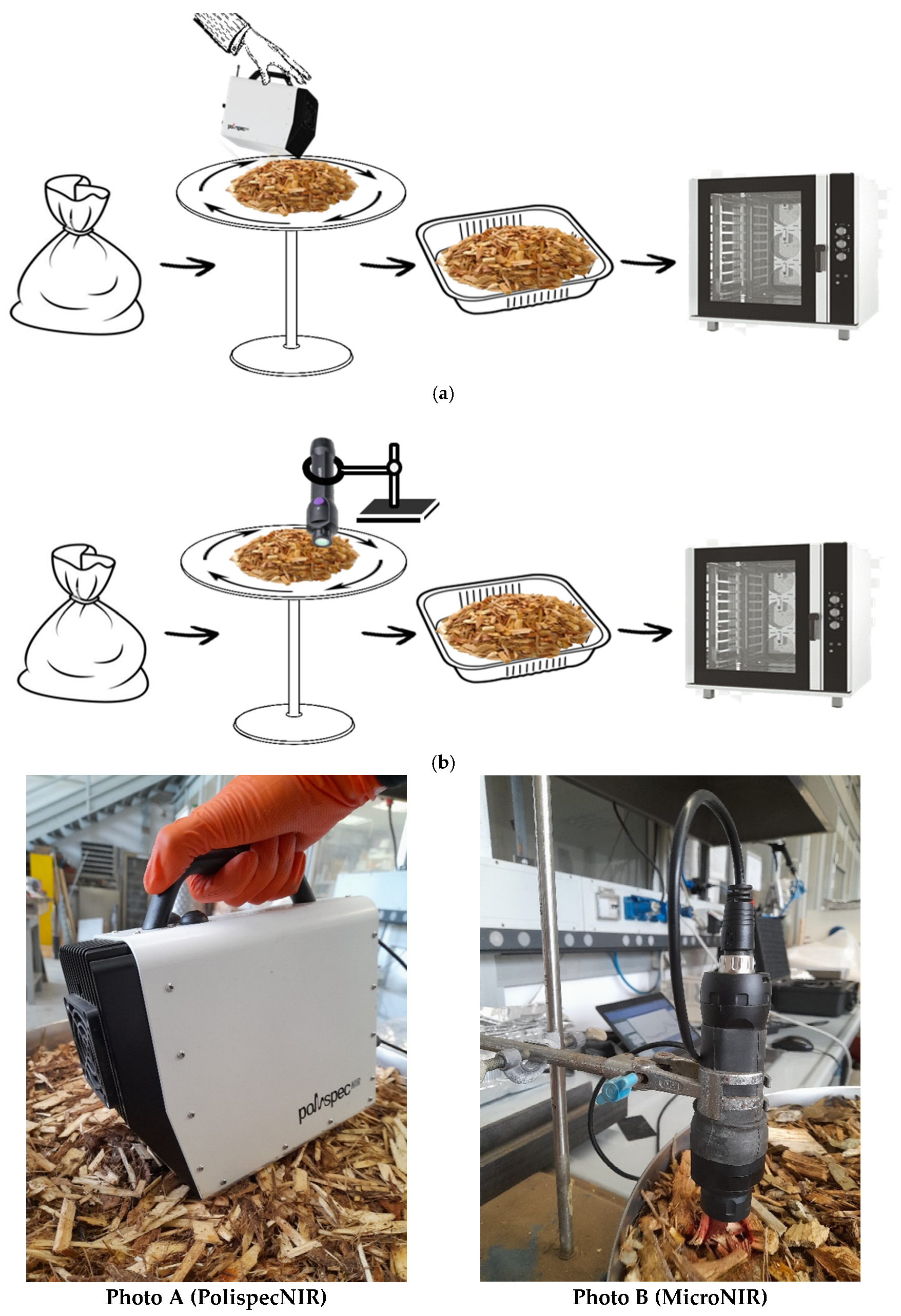
The in-line system performed with the Polispec (Figure 1a), abbreviated as PIL, simulates the spectral acquisition of a multiple swipe with rotatory movement, which occurs when the spectrophotometer slides on the integral woodchip sample poured on a rotating plate entirely covered. Each sample is compounded by the collection of four swipes (as requested by the settings) during the acquisition time of 10 s, resulting in the collection of approximately 46 swipe-scans. For three times (the chosen number of replicates), the material was re-mixed on the rotating plate after each swipe, ensuring consistent sampling and the correct application of the defined method, which expects a triple repetition of the analysis for each sample. Therefore, considering the casual number of spectra collected, the total number of swipe-scans for each sample varies from 118 to 145. As a total and considering the use of 103 samples, the final dataset consists of 14,272 spectra × 256 variables. Moreover, due to the weight of the instrument, the spectrophotometer is held by the operator during the analysis, without a specific and steady support due to its weight as well as its dimension. Therefore, any vibrations resulting from the operator’s inability to maintain a consistent distance from the wood surface may compromise the quality of the acquired data, increasing the spectral noise.
Figure 1.
(a) Schematic representation of the methodology approach for the analysis of woodchip samples using Polispec spectrophotometer for in-line simulation (Photo A). (b) Schematic representation of the methodology approach for the analysis of woodchip samples using Micro spectrophotometer for in-line simulation (Photo B).
In contrast, the in-line system performed with the Micro (Figure 1b), abbreviated as MIL, adopts the same procedure of the Polispec, but the Micro is fixed in a specific point upon the rotating plate by means of metal rod support, constructed in-house. The clamp with screw-on closure locks the spectrophotometer to ensure the keeping of the distance between the woodchip surface and the optic area during the movement. Thus, a distance of about 3 cm, chosen after previous attempts on similar material, was maintained, avoiding the obstruction of the rotational movement for coarser woodchip samples. Moreover, the internal settings were set to collect each spectrum-scan as the average of 1000 scans automatically averaged instead of 100, limiting the external noise related to motion effect. During the analysis, each sample was totally mixed and re-poured on the plate three times, and three more replicates were performed for each re-mix, resulting in nine replicates for each sample. Considering the use of 99 samples, the final dataset consists of 891 spectra × 125 variables.
In both in-line systems (Photos A and B), the mentioned inherent heterogeneity of the industrial woodchip and the consequent variable particle size could prevent direct and neat contact between the superficial layer of woodchip and the optic area of each spectrophotometer. Therefore, the operator is responsible for determining the extent of this detachment, which is based on the trade-off between particle size and the optimal conditions for the best spectral acquisition.
2.4. Spectral Data Processing and Partial Least Square Regression
According to [36], specific Partial least square (PLS) regression models for the prediction of the MC of not-ground woodchips (wet basis) have been already developed and discussed in the case of PIL.
The same procedure was employed in the case of MIL, and three different methods were considered to combine the collected replicates, given their relevance in characterizing heterogeneous samples of the Italian industrial woodchip. In detail: (i) each sample is considered as the average of the nine swipes, obtained by combining three replicates and three swipes per replicate, abbreviated as MET1; (ii) each replicate collected after re-mixing the material on the rotating plate is averaged across its three swipes, abbreviated as MET2; and (iii) each individual swipe is considered a separate sample, abbreviated as MET3. As a result, for each MET (independent from others), PLS models were developed using datasets of different sizes: 99 samples (MET1), 297 replicates (MET2), and 891 swipes (MET3).
According to chemometrics application, each model was validated using venetian-blind cross-validation (using 5 segments) and an external test set. Each dataset was divided into training set (70% of the total) and test set (the remaining 30% of the dataset) using a duplex algorithm [38]. Before the PLS computation, different spectral pre-treatments were applied on the entire spectral dataset to remove scattering and baseline effects, minimizing the noise presence. In detail, scatter correction pre-treatments (standard normal variate, abbreviated as SNV, and multiplicative scatter correction, abbreviated as MSC) and first and second derivatives (Savitzky–Golay filter, 9, 13 or 21-points window, 2nd-order polynomial filter) were performed and compared. Moreover, as mentioned above and according to each MET definition, samples were averaged across replicates, assuming that the replicates belonging to a specific sample had been kept together and avoiding the incorrect placing into both training and test set. Next, for each pre-treatment, cross-validation was applied on the training set to construct the model, before using the test set to validate it. Moreover, regression plots, PLS score plots and X-Y influence plots (residual vs. leverage) were analyzed to detect possible outliers.
In order to compare models’ performance, corresponding statistics were recorded: the determination coefficient in cross-validation and in validation (respectively, R2cv and R2val), the error both in cross-validation (RMSECV in %) and in validation (RMSEP in %), together with the range to error ratio (RER) and the ratio of standard error of prediction to standard deviation (RPD) calculation. These indices permit one to set out a reliable indication about the prediction goodness; according to Williams and Norris [39] and confirmed by the cited authors [40,41], RER values should be between 7 and 20 to exploit the model in quality screening applications, while greater than 20 for any quality control applications. In contrast, RPD should be greater than 3 only for screening applications and greater than 5 for quality control applications [32,42,43].
All the computations were performed in a Matlab environment (ver. 7.10.0, The MathWorks) using in-house functions on existing algorithms.
2.5. General Statistics and Comparative Processes
Different statistical and comparative analyses were performed on the MC parameter for each MET. Starting from general statistical analysis, average, standard deviation, and minimum and maximum values were calculated for each dataset, leading to the initial representative evaluation of their inherent variability and their consequent perspective on the Italian industrial woodchip received by power plants.
Furthermore, the Prediction Range Definition (PRD) was carried out for each dataset to evaluate the performance of each model in closely predicting the MC value compared to the measured one obtained with standard analysis. Therefore, the bias, defined as the difference between predicted and measured MC value, was calculated and classified according to specific classes, using a defined threshold as tolerance limit (Table 2) to assign a score that increases with the deviation. Those limits were set a priori by the authors according to the experience acquired in power plants (i.e., during sampling), the feedback from sector operators, and the comparation with historical datasets for the same type of material.
Table 2.
Established ranges, used as tolerance limits, applied for the four classes to classify samples according to MC bias.
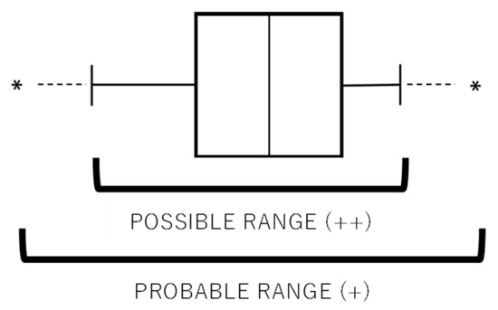
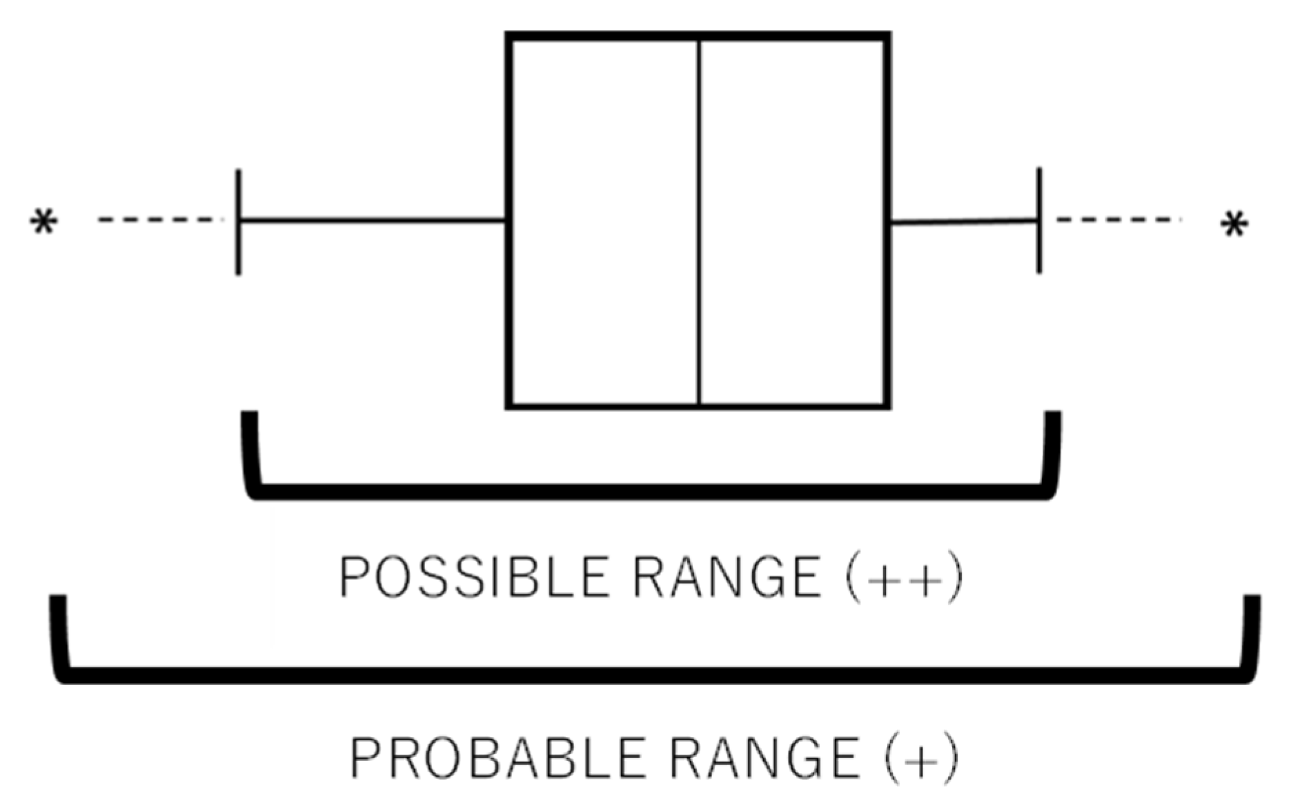
Lastly, to identify the number of significantly different individual means from a set of means, the multiple comparison test of Tukey’s Test (abbreviated as TT) was performed. Starting from the definition of the set as the collection of predicted MC values for each sample according to MET3, TT calculates the minimum and maximum value of both the inner and outer limit of each set. Therefore, the application of TT permitted us to establish the number of outliers classified as probable and possible. The former are placed in the outer portion of fences (related to the specific definition of extreme, equivalent to Q1 ± 3 × IQR), while the latter are placed in the inner portion of the same fences (related to the specific definition of suspected, equivalent to Q1 ± 1.5 × IQR).
Thus, the removal of probable outliers (abbreviated with “+” symbol) means a minor intervention in the dataset, whereas the removal of possible outliers (abbreviated with “++” symbol) is equal to a higher degree of intervention and dataset modification. As a result, TT allowed the assessment of the degree and the influence of replicates in the definition of the dataset’s variability thanks to the application of these two severity approaches (Figure 2).
Figure 2.
Graphical representation of a box plot that defined two different ranges adopted for the outlier removal during TT application. The symbol * represents the highest distance in which an outlier could be detected.
3. Results
3.1. Raw Spectra Evaluation
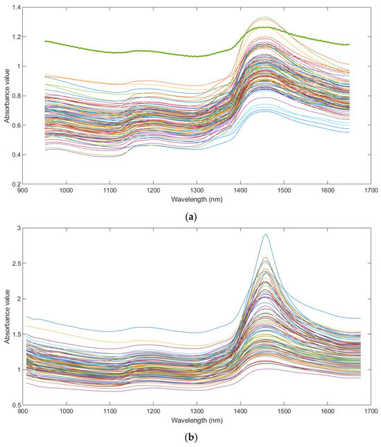
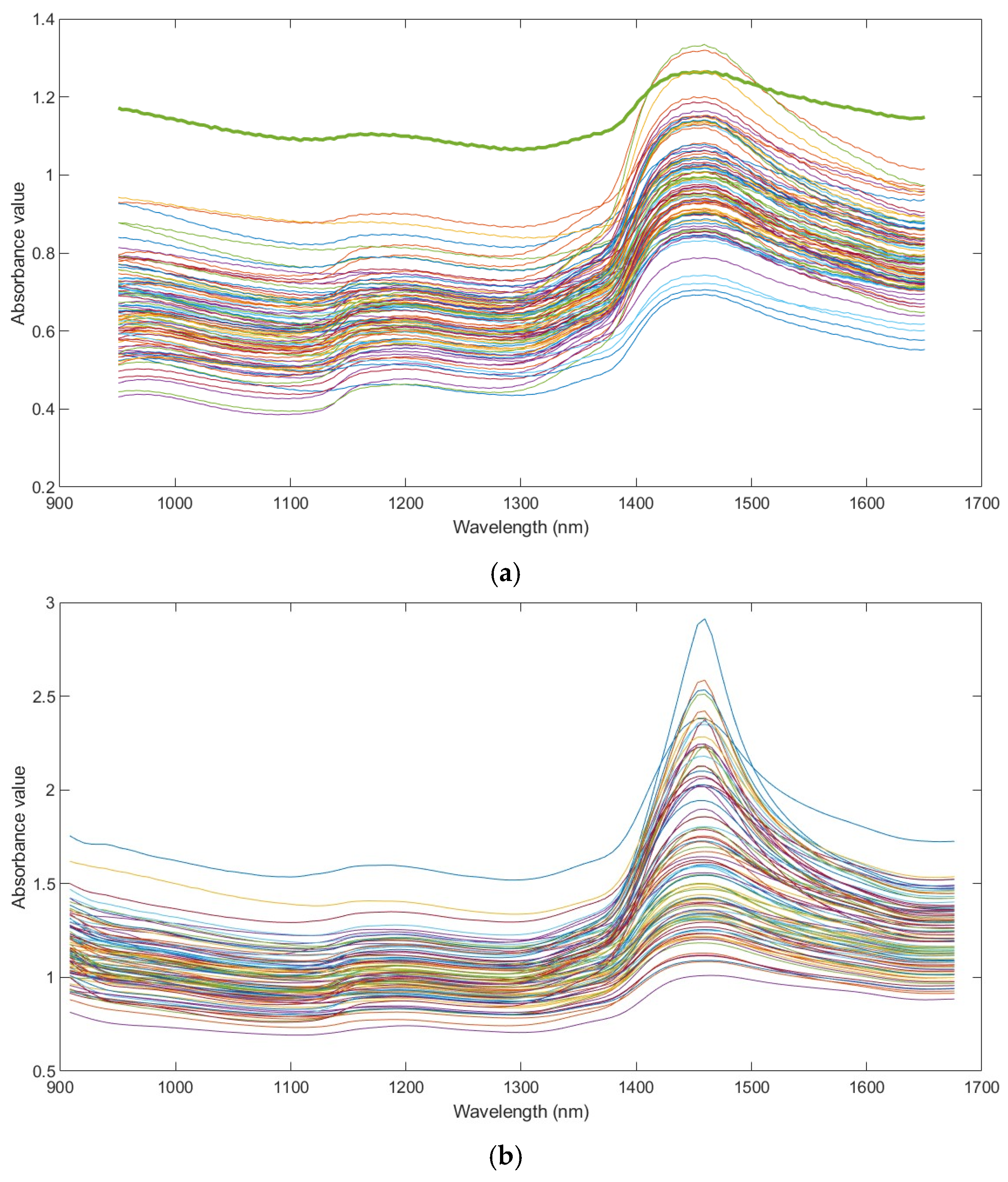
The averaged raw spectra through replicates of the analyzed woodchip samples of D-PIL and D-MIL have been compared and are shown in Figure 3a,b. Taking into account the similarities between analysis methods, the material investigated, and the acquisition process, this comparison leads to the identification of those differences that might relate to the technical settings of the instruments.
Figure 3.
Averaged spectra (across replicates) for both the D-PIL dataset (a) and the D-MIL dataset (b). The spectrum in D-PIL, considered noisy and removed, is underlined in bold green (a). The difference in absorbance magnitude values is related to manufacturing specifications of spectrophotometers.
Averaged raw spectra from D-PIL (Figure 3a) shows the relevant presence of noise, related not only to the inherent heterogeneity of the woody material, but mainly to the influence of external conditions. In fact, the lack of direct contact between the first layer of the wood surface and the acquisition window of the spectrophotometer, together with the lack of operator stability in holding the instrument during collection, increases the negative interaction with the external light, causing a scattering effect. For this reason, 33 extreme variables have been removed due to the high spectral noise, considering 950–1650 nm as the new spectral range. Moreover, one averaged spectrum (bold in green in Figure 3a) has been detected and removed due to its isolated position compared to the entire spectral group.
On the contrary, averaged raw spectra from D-MIL (Figure 3b) appear smooth and spectral noise is not easily detected, so neither wavelengths nor outlier spectra have been removed. In this case, the metal rod support used for Micro contributes to being able to strongly hold and keep stable the spectrophotometer, stabilizing the acquisition. Nevertheless, both datasets present similar spectral shape and a relevant peak between 1400 and 1500 nm, clearly evident in D-MIL due to the potentially higher MC value of woodchip samples collected during autumn and winter conditions, as reported in Table 1. In fact, the peak is related to water content, specifically to the first overtone (OT) of the O-H stretching bond [44].
3.2. Prediction of Moisture Content of D-MIL with In-Line Simulation
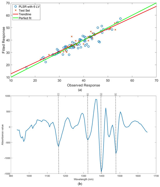
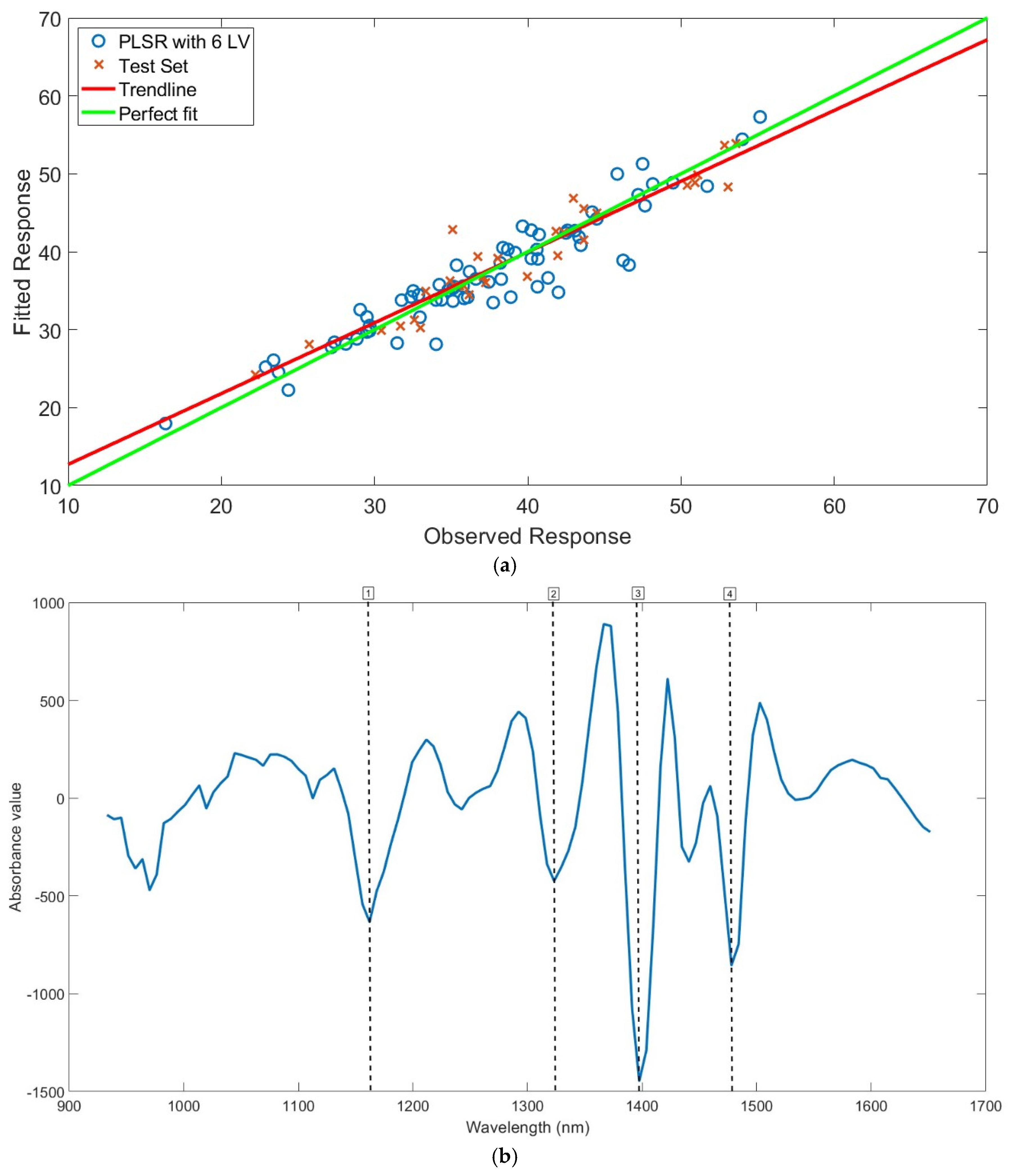
Based on MIL, PLS regression models have been developed for the prediction of MC, and the results are shown in Table 3, Table 4 and Table 5, respectively, for MET1, MET2 and MET3. From the investigation of the raw spectra (Figure 3b), improper spectral shapes were not detected, so all the spectra have been considered in the model development. For MET1, 69 samples have been used as the training set, and the remaining 30 samples as the test set for the validation step. The best performance has been obtained using the derivative as spectral pretreatment (second derivative with Savitzky–Golay filter, nine-points window, second-order polynomial) (Table 3). Moreover, no sample outliers have been removed after the investigation of residual/leverage plot, coupled with the observed/predicted response, as well as the score plots. The model used six LVs and returned R2cv = 0.88, RMSECV = 2.65%, R2val = 0.91, and RMSEP = 2.37%, while the calculation of RER and RPD attained 13.22 and 3.37, respectively, attesting its potential implementation for direct, but not practical, application. The model performance is also represented by the regression plot (Figure 4a), that shows how the trendline fits with the perfect fit, and by the corresponding regression vector plot (Figure 4b), where the most significant wavelengths responsible for the MC prediction are highlighted. In particular, four relevant negative peaks (due to the spectral pretreatment of second derivative applied) have been detected. The peak at 1162 nm (1) could be related to C-H bonds, probably due to (i) combination bands that occur between first- and second-order deformation, or to (ii) second-order stretching bands [45]; the peak at 1329 nm (2) could be related to the stretching and deformation of C-H bonds [35]. Otherwise, the peak at 1397 nm (3) is considered the most relevant of the group and it could be related to the first OT of C-H combination bands, together with the first OT of O-H stretching vibrations, so confirming the relevant detection of water content [30,46]. Lastly, the peak at 1477 nm (4) is also related to water presence because it could be assigned to the first OT of O-H stretching bonds of cellulose [43].
Table 3.
Main results of the PLS regression models developed for the prediction of MC for MIL, considering MET1. The best model is highlighted in bold.
Figure 4.
(a) Partial least squares (PLS) regression plot (RP) for the prediction of MC according to MET1 for D-MIL. Spectra were pre-processed by second-order derivation using the Savitzky–Golay algorithm with 9 smoothing points and 6 latent variables. The observed and fitted responses are represented by MC values (%); (b) corresponding regression vector plot (RVP) using dashed vertical lines, with corresponding numbers to highlight the most important wavelengths.
For MET2, the best model was developed pretreating the spectra with the second derivative (Savitzky–Golay filter, nine-points window, second-order polynomial). Also in this case, no sample outliers have been removed during PLS computation. As highlighted in Table 4, the dataset has been divided into 207 and 90 samples for the training and the test set, respectively, and the model uses five LVs, returning R2cv = 0.88 and RMSECV = 2.68%, and R2val = 0.88 and RMSEP = 2.74%. RER = 11.43 and RPD = 2.92 confirm the same potential implementation in direct application of MET1, despite a little lower performance, precluding practical use. Similarly, Figure 5a shows the regression plot, while Figure 5b the corresponding regression vector plot of the best model, with highlighted the most relevant wavelengths for the prediction of MC. According to spectral pretreatment of MET2, three negative peaks have been considered, despite the peak at 1155 nm (1) not being considered as relevant as the others. In particular, this peak could be related to the second OT of C-H stretching vibrations of hemicellulose [44]. The most relevant peak at 1397 nm (2) could be related to O-H and C-H stretching vibrations [28], in particular to C-H stretching and deformation [46], while the peak at 1477 nm (3) could be related to the first OT of O-H stretching bonds [44], associated with lignin presence [43].
Table 4.
Main results of the PLS regression models developed for the prediction of MC for MIL, considering MET2. The best model is highlighted in bold.
Figure 5.
(a) Partial least squares (PLS) regression plot (RP) for the prediction of MC according to MET2 for D-MIL. Spectra were pre-processed by second-order derivation using the Savitzky–Golay algorithm with 9 smoothing points and 5 latent variables. The observed and fitted responses are represented by MC values (%); (b) corresponding regression vector plot (RVP) using dashed vertical lines, with corresponding numbers to highlight the most important wavelengths.
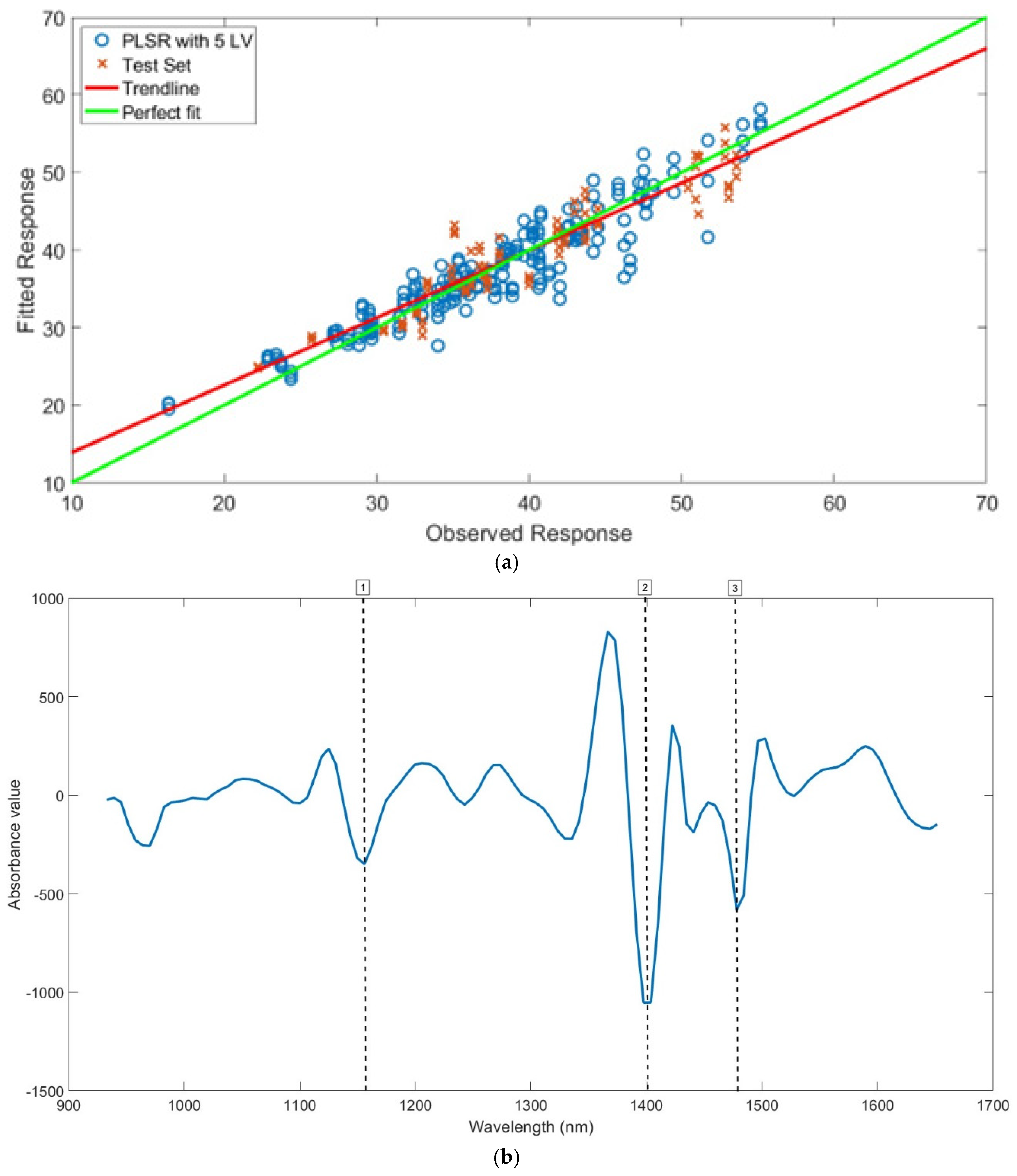
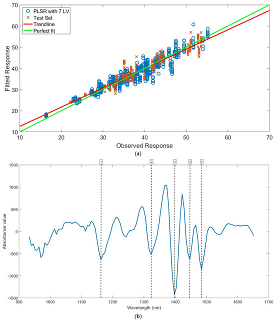
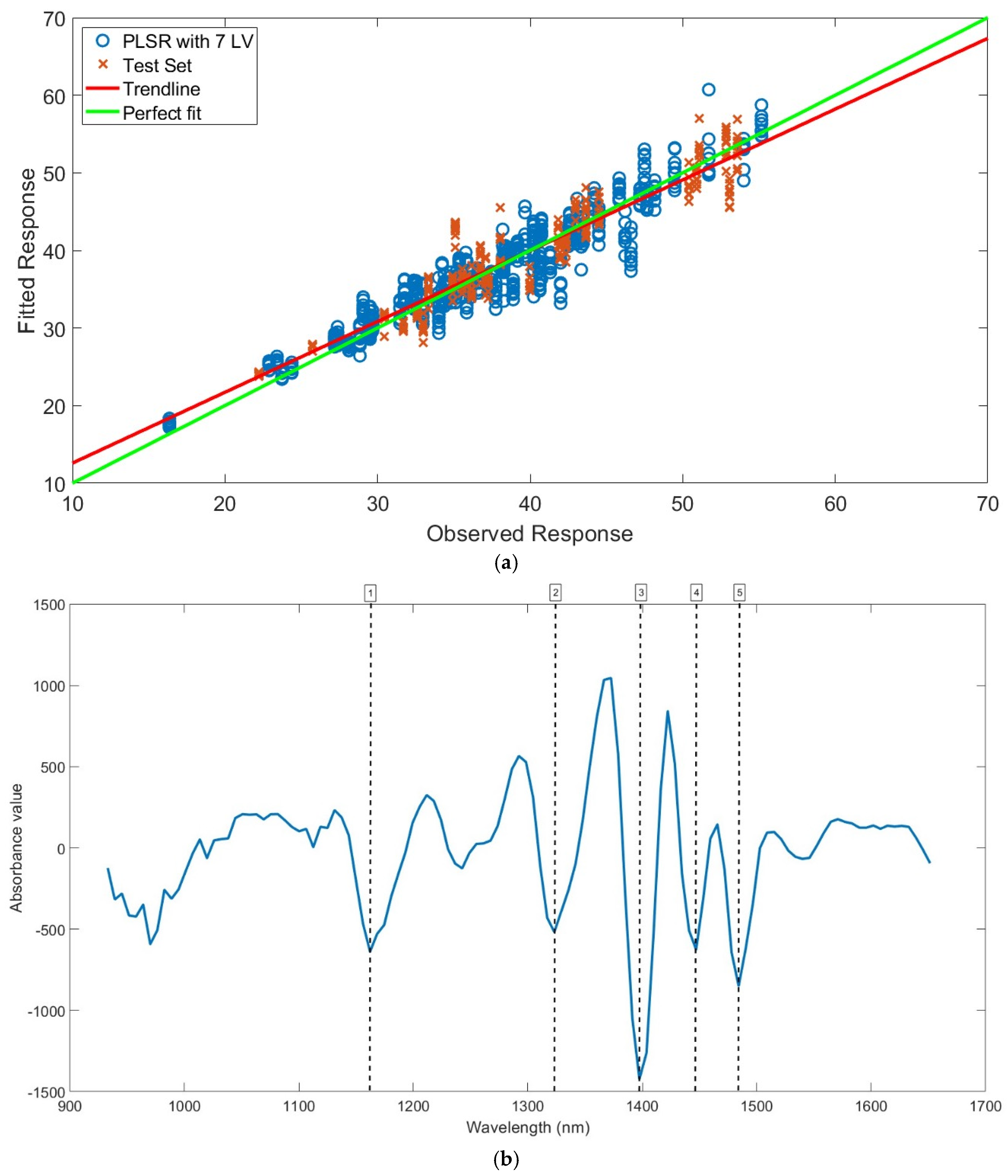
Lastly, the best model for the prediction of MC with MET3 was developed pre-treating the spectra with the second derivative (Savitzky–Golay filter, nine-points window, second-order polynomial). Contrary to MET1 and MET2, three sample outliers have been removed; in particular, one sample outlier has been removed from the training set, while two sample outliers have been deleted from the test set during PLS computation by investigating residual/leverage plot, the observed/predicted response, but also the PLS score plots, obtaining a total of 888 samples divided into 620 and 268 samples for the training and the test set, respectively. As reported by Table 5, the model uses seven LVs and returned R2cv = 0.90 and RMSECV = 2.42%, and R2val = 0.89 and RMSEP = 2.69%. The values of RER = 11.67 and RPD = 2.96 confirm similar performances compared to MET2. Again, Figure 6a shows the regression plot while Figure 6b the corresponding regression vector plot, highlighting the most relevant wavelengths for the prediction of MC. In particular, the peak at 1397 nm (3) could be associated with the same peaks detected in MET1 and MET2, confirming the significant and valid identification of water content. Even the peak at 1162 nm (1) could be referred to the same peak detected in MET1 and related to combination bands of C-H. Moreover, the peak at 1323 nm (2) could be related to CH3 groups of lignin and hemicellulose [28], while the peak at 1447 nm (4) could be related to the phenolic hydroxyl groups in lignin (aromatic structure) [44]. Lastly, the peak at 1484 nm (5) could be related to the first OT of O-H stretching bonds in the crystalline region of cellulose [26].
Figure 6.
(a) Partial least squares (PLS) regression plot (RP) for the prediction of MC according to MET3 for D-MIL. Spectra were pre-processed by second-order derivation using the Savitzky–Golay algorithm with 9 smoothing points and 7 latent variables. The observed and fitted responses are represented by MC values (%); (b) corresponding regression vector plot (RVP) using dashed vertical lines, with corresponding numbers to highlight the most important wavelengths.
Table 5.
Main results of the PLS regression models developed for the prediction of MC for MIL, considering MET3. The best model is highlighted in bold. Rightly, the MEAN is not considered.
The most relevant peaks detected in each MET correspond to OH bonds of the main wood component, namely cellulose and hemicellulose. Therefore, water content is identified within the NIR spectral range, confirming its reliability in detecting such a crucial physical parameter for the characterization of woody biomass.
3.3. General Statistical Analyses
General descriptive analyses have been performed to extract the main information about the D-MIL woodchip analyzed. Furthermore, assuming that the origin of the woody material within the same year of collection is maintained unchanged [13], as confirmed by t-test result, the D-MIL is compared to the D-PIL, already investigated and presented [36]. Moreover, the comparation of each approach of analysis (PIL and MIL) with the results obtained through the standard methodology (STD) for the measurement of MC (according to ISO 18134) also permits us to assess the annual variability of this parameter for the traded Italian industrial woodchip. All the results are shown in Table 6.
Table 6.
Descriptive statistics for MC parameter on woodchip samples collected for both D-MIL and D-PIL, coupled with the respective results of MC measured with standard analysis.
For both approaches, each MET shows very similar results compared with the corresponding MC value from standard lab analysis. Despite the slightly higher mean values observed in D-PIL, in particular for MET3 (40.17% vs. 39.99%), the difference with the measured MC in D-MIL is considered trivial (<1%) and could be given by the natural heterogeneity of industrial woody material. Standard deviation values of each MET follow the same pattern of mean results, confirming the higher discrepancy of MET3 of D-PIL compared to others (5.95 vs. 7.59) despite the wider range value of MET3 next to MET1 and MET2, and probably associated to the worse model’s performance that struggles to propose a more correct data representation. Instead, the minimum and maximum values are extremely few compared with the percentages of samples belonging to central classes (7.69% for MC < 30% and 6.72% for MC > 50% vs. 85.59% for MC between 30 and 50%). Nevertheless, it reached a closer range value to the standard analysis result, due to the overestimation of lower MC. In contrast, the range value of MET3 of D-MIL is the furthest, even if closer minimum and maximum MC values are detected, pointing out a relevant difference in operative approach between instruments. Considering the whole statistics, MET3 of D-PIL seems to be influenced by the huge number of replicates collected during the analysis with a more unstable acquisition mode that could increase the spectral noise, limiting a more correct dataset representation.
Although these fluctuations in MC detection between datasets are not considered significant, several factors could affect this variability, starting from the ordinary fluctuations of climatic conditions within seasons to the occurrence of more intense/frequent rainfall events. Furthermore, sampling procedures, as well as the material handling from the harvest process up to the storage, could influence the material characteristics and, above all, a different timing of drying. Anyway, based on the results of the standard analysis, the qualitative characteristics of the woodchip samples employed is maintained, suggesting that the biomass used for energetic purpose in Italian power plants is not subjected to relevant variations within a year, ensuring a stable flux of ready renewable resources. This was also confirmed by the great MC monitoring of Italian industrial woodchips carried out during the 2019–2023 period for the same regions of interest [13].
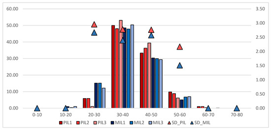
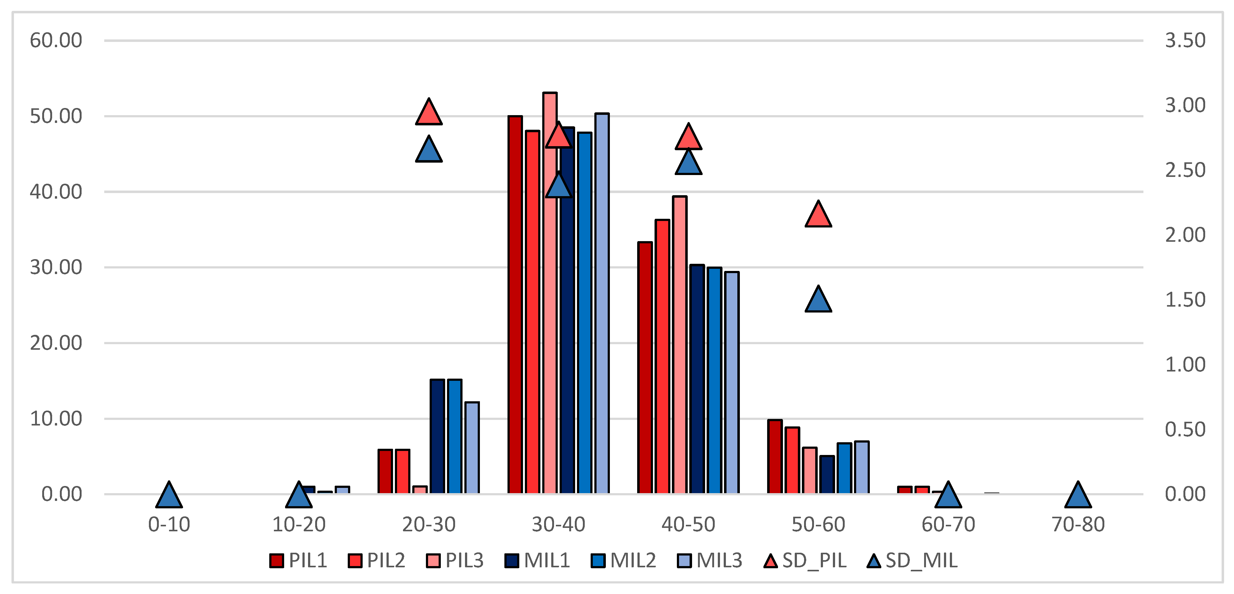
Therefore, Figure 7 compares the D-MIL and D-PIL distributions according to MC classes of 10% range. Most of the samples are distributed in central classes (30–50%) while only a minimal part is placed in extreme classes (0–20% and 60–80%), confirming the statistic results (Table 6) and the expected values of MC for the woodchip handled by the Italian power plants.
Figure 7.
Graphical distribution of samples, expressed in percentage (%), in classes of MC (block of 10% as range) for D-MIL (MIL1, MIL2, and MIL3) and D-PIL (PIL1, PIL2, and PIL3). The light blue and the light red triangles correspond to the distribution of the samples according to the results of standard analysis for D-MIL and D-PIL, respectively.
D-MIL samples tend to take place in lower MC classes (10–30%), while the inverse trend is evident for the D-PIL samples (50–70%), confirming the slightly higher MC mean values for D-PIL that are related to season and management influence. In general, the smallest differences are detected in the 30–40% class, which contains the largest percentage of samples closely matching the standard analysis distribution (the average value of 50.37% of presence for D-PIL, and the average value of 48.88% of presence for D-MIL). However, major differences between D-MIL and D-PIL are shown in intermediate MC classes. In the 20–30% class, a higher presence of D-MIL samples is detected, confirming a valid prediction of dryer samples and the minimum values resulted. On the contrary, a good presence in the 50–60% class, and their absence in the 60–70% class, validate their efficiency in predicting the complete MC range, congruent with the actual MC distribution (from 16 to 55% of water measured). An inverse trend is spotted for D-PIL, with a small presence of samples in the 20–30% class and a more relevant presence in the 50–70 range, supporting the MC range of its dataset (from 17 to 60% of water measured). Again, the MET3 of D-PIL shows a more unstable distribution, revealing a distinct pattern compared to MET1 and MET2 in each class, due to the huge number of scans in less steady condition that could negatively affect the prediction of MC along its normal distribution. Lastly, the differences in standard deviation values (illustrated in blue for MIL and in red for PIL) are mainly detected in the 50–60% class (2.17 vs. 1.51 for PIL and MIL, respectively) and in the 30–40% class (2.78 vs. 2.39 for PIL and MIL, respectively). In the other classes, despite being more moderate, higher degrees of dispersion for PIL are recorded, confirming the unfavorable effect of an excessive number of replicates in that condition.
3.4. Prediction Range Definition
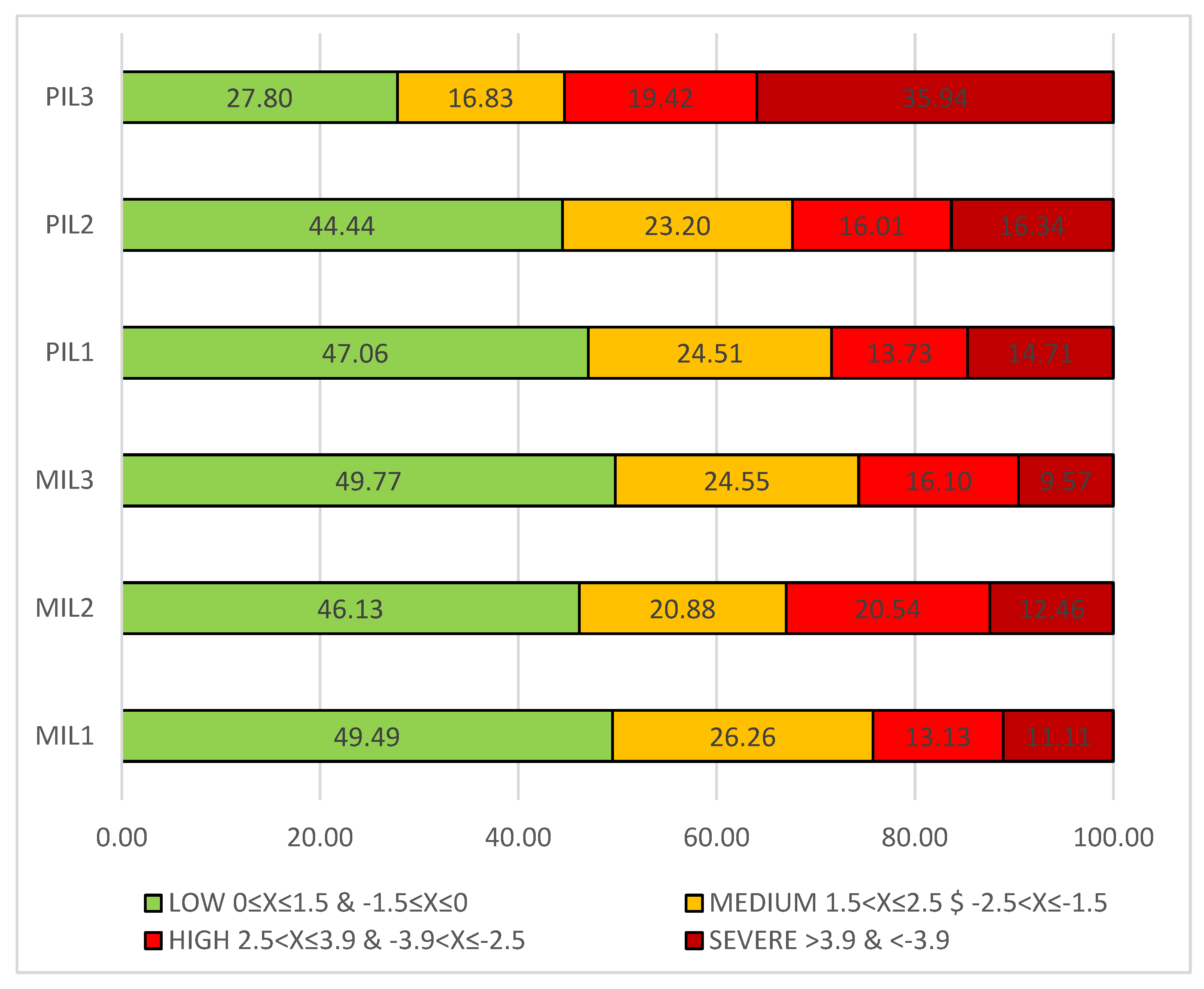
The calculation of bias, defined as the difference between the predicted and the measured MC values, leads to the definition of a tolerance limit aiming at assessing the accuracy of prediction, but also to establish the range within which the operator could consider tolerable the estimation of MC, particularly to improve direct implementation of immediate evaluation in power plants. As already developed with the results for D-PIL [36], the D-MIL samples have been distributed in four different classes of tolerance (Table 2), which have been arbitrarily chosen, evaluating the bias performed during estimation. The results, expressed as percentages based on the total number of samples considered, are illustrated in Figure 8.
Figure 8.
Graphical distribution of the number of samples according to the defined classification of PRD classes related to bias in prediction, for each MET and for both instruments. The distribution is represented by %. Positive and negative samples, related to positive and negative bias respectively, are counted together.
Except for PIL-MET3, where spectral noise could cover information and cause anomalous trends (as shown in the graphical representation of Figure 8), the major part of samples is placed in the green group (low-class, equal and/or less than 1.5%). The poorer performances are related to the high number of samples classified in the severe class, due to a relevant distance between the predicted and the standard MC value. On the contrary, the small presence in the severe class, linked to a greater assignment in low-class (more than 50% of the total dataset), validates the good performance in predicting MC values. While the other METs both for PIL and MIL present comparable class attributions, the MET3 of PIL achieved the worst performance, with about half of the samples located in low-class and almost a double presence in severe-class compared to MET1 and MET2. Once again, the discrepancy of its performance confirms that collecting an excessive number of replicates with high spectral noise may adversely affect the model’s predictive ability. In contrast, the MET3 performance of D-MIL exhibits the highest percentage of samples in low-class (49.77%) and the lowest in severe-class (9.57%). Moreover, patchy results are found for medium- and high-class in the MIL approach. For example, MET2 presents a smaller medium-class percentage (20.88%) but also a larger high-class percentage (20.54%). The opposite pattern corresponds to MET1, suggesting a quite equal trend compared to MET3. Excluding MET3, the MET1 and MET2 of PIL present irregular conditions: their percentages of presence in medium- and high-class are similar to MIL, but severe-class presence is greater in both cases, reducing the reliability of their performances. Nevertheless, this divergence is considered unremarkable because it is primarily related to the heterogeneity of such a natural and variable category of industrial woodchip samples.
3.5. Tukey’s Test
The results collected from the application of Tukey’s Test (TT) permit an explanation of how the collection of replicates could influence the model’s performance. Starting with the bias calculation, the test defines:
- -
- Better samples: When the removal of replicates belonging to a sample decreased the bias, resulting in a predicted MC closer to the measured MC;
- -
- Worse samples: When the removal of replicates belonging to a sample increased the bias, resulting in a predicted MC far from the measured MC.
Thus, as described in Section 2.5, the number of replicates considered as outliers has been established according to two different degrees of intervention or severity: (i) minimum severity (+), when the removal of replicates involves probable outliers (due to the extreme MC with respect to the mean value), and (ii) maximum severity (++), where the removal of replicates involves possible outliers (that means that replicates are located in an intermediate “distance” between the mean value and the probable outlier). Table 7 shows the results of TT, computed considering all the replicates collected with MET3 of both D-MIL and D-PIL, but the results are presented as a percentage of the total (103 for D-PIL and 99 samples for D-MIL).
Table 7.
Brief table of TT results for D-MIL and D-PIL, considering the replicates collected according to MET3. Each value corresponds to the % of samples, on the averaged samples, affected by the outliers’ removal, and not the number of samples eliminated.
Considering the application of + severity that removed the probable outliers, the results show that in D-MIL, in contrast with D-PIL, the % of samples in which outlier removal reduced the bias (“better”) is less than the % of samples with worsening of bias (“worse”), reducing the performance (2.02 vs. 7.07% for D-MIL, while 12.62 vs. 9.71% for D-PIL). The same trend is evident in the ++ severity, that adds the removal of possible outliers (11.11 vs. 14.14% for D-MIL, while 48.54 vs. 41.75% for D-PIL). This result could suggest the higher variability of D-PIL compared to D-MIL, because of the greater presence of noisy scans collected. Their removal, considering their potential disturbance role and their reduced significance among a sizeable group (about 139 MC values for each sample), could act as a model’s improvement. Therefore, the removal of probable and possible outliers in nine MC values for each sample, considering TT application on the MIL approach, could implicate a major impact, resulting in a worsening effect.
Nevertheless, the number of samples where the probable outliers removal occurs (either positively or negatively) is very low in both datasets (9.09% and 22.33% for D-MIL and D-PIL, respectively), resulting in 90% of no-impact samples for D-MIL and in about 78% for D-PIL. The relevant difference occurs with the application of ++ severity in D-PIL, due to the huge % of samples with outliers (90.29%) that leads to less than 10% of no-impact samples, compared to the 74.75% of no-impact samples for D-MIL. However, allowing the admission of a minimum bias of 0.5% instead of 0 for each severity degree, both datasets result in greater performances (more than 98% of no-impact samples for + severity and about 97% for ++ severity). Considering the outliers evaluation as a demanding and time-consuming step and facing the natural variability of Italian industrial woodchip, the acceptance of a minimum range of error could permit more direct characterization, enhancing immediate results, real-time assessment, and lower risks of improper MC definition.
4. Discussion
The application of the NIRS technique, given the in-line simulation rendered in laboratory, provides valuable insights into the advantages and limits of its potential implementation directly in power plants. Actually, the use of two different spectrophotometers, distinct in their technical characteristics but employed in the same analytical approach, permits an exhaustive comparation aimed at identifying: (i) the most effective monitoring system based on operative requirements, and (ii) the suitable location of the spectrophotometer for its potential implementation along the supply chain, considering the parameter investigated.
Therefore, the combination of the analyses carried out works for offering a comprehensive overview of the strengths and weakness of the MIL and PIL approaches. Starting from the comparation between the PLS model performances for each MET (Table 8), the MIL system generally shows superior results, shown by higher values of the R2cv/val, RER and RPD parameters, combined with lower error values.
Table 8.
Comparative scheme of the results of PLS prediction models for the MC parameter applying two different portable NIR spectrophotometers.
If the performance of each MET of MIL could be considered quite similar, the results of the MET3 of PIL notably decreases compared to MET1 and MET2, confirming the poorer performance (RER = 7.48 and RPD = 1.67) also detected during PRD and TT execution and in statistics. In fact, the MC standard deviation of MET3-PIL (5.95) results are lower than the value from standard analysis (7.59), and other METs (7.35 and 7.28), also confirmed by its lower coefficient of variation (calculated as the ratio of the standard deviation to the absolute value of mean) of 0.148, compared to 0.190 of standard, 0.184 of MET1 and 0.182 of MET2. In contrast, the coefficient of variation for D-MIL, equal to 0.206 for standard, ranges from 0.195 (MET2) to 0.202 (MET1), revealing a limited variation between them. The irregular trend of the MET3 of Polispec is also notable in class distribution, registered in a larger number of samples with severe bias, and combined with the reduced ability to accurately predict MC. Therefore, it seems that the large amount of data collected with the PIL approach, without a steady support, could increase the acquisition of noise and scattered data, rather than provide a more thorough description of material heterogeneity, due to the instability of the measurement in this condition. Nevertheless, the TT analysis would suggest that, despite the higher number of outliers identified with PIL, the acceptance of a minimum error (0.5%) leads to stronger performances, comparable with MIL (98.99 and 96.97 for MIL vs. 98.06 and 97.09 for PIL, for + and ++ severity, respectively). This achievement could also positively face the relevant influence of the natural heterogeneity and variability of industrial woodchip, resulting in a more appropriate and complete representation of the material flow in each step of the supply chain.
Considering the obtained results and assuming the necessary utilization of RES and the critical importance of biomass characterization, a brief but practical guide could be suggested, to better support and improve the most suitable energy production system. Reliable prediction models of MC have been successfully developed with both spectrophotometers, but technical and operational aspects could influence the choice of the implemented instrument. In detail, the lighter weight of Micro, compared to Polispec, makes it more suitable for complex sampling or in situations with limited mobility. Nevertheless, the lack of Bluetooth connectivity in the Micro used in this research makes Polispec more appropriate for field activities, for its integration into production lines, where the remote control became fundamental. Furthermore, technological innovation could readily supply an upgraded spectrophotometer with Bluetooth connection, enhancing flux management, operative asset, and additional equipment costs. Both spectrophotometers could be easily applied to ground material, while surmountable difficulties have been met with unground material, due to the rough and jagged granulometry of industrial woodchip. In fact, the coarse part of the material poured onto the rotating table collided with the external case of the instrument, forcing the operator to lift it from the surface, and thus increasing the susceptibility to external light interference. However, additional accessories may address this limit, like boosting the power of the light beam and combining it with a narrow eye to make it more punctual but also improving averaged single scan collection to maintain the flow effect. Moreover, a dark tunnel could be placed along the chain, shielding the spectral collection moment from external influence without interrupting the material flux, promoting direct applications in power plants. Further, when heavier instruments cannot be held up with an external system to improve steadier acquisitions on irregular materials, their application could be dedicated to more homogeneous materials, such as pellets and milled woody biomass, that favor less external interference with the reduction of the minimum distance from the material.
5. Conclusions
These findings confirm the significant advantages of in-line implementation of the NIRS technique in power plants for qualitative monitoring of moisture content, thanks to its non-destructive, rapid, and cheaper assessment compared to standard analysis. NIRS results a valuable tool for providing real-time control of material characteristics, while preserving the chemical and physical properties of biomass. The predictive capacity of NIRS to provide a qualitative-screening tool is effectively demonstrated for the MC parameter, leading to the development of different prediction models that represent a crucial step to extract meaningful information from qualitative and quantitative data, translating into intuitive and user-friendly tools for the operators. To this end, a portable spectrophotometer has been employed in a simulated in-line system, applying three approaches based on replicate combinations (METs), and then compared with a different portable NIR handled with the same operative approach. The best PLS models return R2val = 0.91, RMSEP = 2.37%, RER = 13.22, and RPD = 3.37 for MicroNIR (MET1), while R2val = 0.86, RMSEP = 2.88%, RER = 11.52, and RPD = 2.63 for PolispecNIR (MET1). Nevertheless, similar performances have been reached also with MET2 and MET3 using D-MIL, while only MET2 of D-PIL showed affordable and comparable values, while MET3 recorded poorer results. The findings suggest the importance of replicate collection to adequately capture the whole biomass heterogeneity, but also it is recognized that the collection of replicates, without rigorous control of the stability conditions, could introduce important spectral noise that negatively compromises the models’ performance because of the hidden key information. Indeed, PRD results confirm that the outsized collection of “dirty” measurements has a negative impact on models’ applicability, increasing bias and reducing reliability (for example, comparing MET3, the samples classified as low-class are 49.77% vs. 27.80%, respectively, for MicroNIR and PolispecNIR, while 9.57% vs. 35.94% are severe-class, respectively, for MicroNIR and PolispecNIR). Lastly, the negative effect of the uncontrolled collection of replicates is even confirmed by TT results, where PolispecNIR reveals higher percentages of identified outliers compared to MicroNIR (22.33% vs. 9.09%, respectively, considering a lighter degree of severity). Nevertheless, the tolerance of a minimum bias error can effectively face the huge variability in Italian industrial woodchip composition, allowing a more accurate representation of its inherent heterogeneity, but also the attenuation of sampling error and detrimental storage effects. As a result, if more than 96% of samples do not require outlier removal for both instruments, effective real-time control could enhance material characterization, minimizing the need for dataset manipulation and saving time, and also driving a wider circulation of industrial woodchip as a renewable energy resource.
Despite different performance levels that required further validation, both PolispecNIR and MicroNIR prove to be valid instruments to develop accurate MC prediction models, offering important advantages in analyzing material flow in outdoor environments and power plant conditions. Due to its relevant weight, PolispecNIR may require specific attention, including the utilization of additional devices to ensure the optimal stability during spectral acquisition. By the way, the compact hand-case and the ergonomic design of both instruments make them also suitable to being moved between dusty and dirty environments, as well as to be steady-implemented at critical points along the production line. A continuous monitoring could be also a guarantee, thanks to the non-stop data collection and the unnecessary operator assistance. The exploitation of an automatized system as continuous control of incoming feedstock could minimize running costs, enhancing an extensive placement of monitoring devices, e.g., along the conveyor belt towards the furnace, at unloading points of trucks, or for periodic checks on storage piles. As an example, the real-time assessing of moisture content could prevent incorrect economic transition based on load weight instead of the potential energy content of the biomass. Moreover, the successful implementation of NIRS in both in-line and point-based processes could enable the rapid characterization of biomass properties and the continuous control of loads, facilitating the identification and resolution of potential bottlenecks along the supply chain, thus improving economic and environmental benefits.
Author Contributions
Conceptualization: E.L.; Data curation: E.L. and M.M.; Formal analysis: E.L.; Investigation: E.L.; Methodology: E.L.; Project administration: E.L., M.M. and D.D.; Resources: E.L. and T.G.; Software: E.L., M.M. and T.G.; Validation: E.L., M.M. and T.G.; Visualization: E.L., L.O. and D.D.; Supervision: T.G. and M.M.; Writing—original draft: E.L.; Writing—review and editing: E.L., M.M., T.G., L.O. and D.D. All authors have read and agreed to the published version of the manuscript.
Funding
This research received no external funding.
Data Availability Statement
The raw data supporting the conclusions of this article will be made available by the authors on request.
Acknowledgments
The authors are grateful to ITPhotonics S.r.l. Italia for technical support and also for permitting the rent of PolispecNIR during the analysis for the simulation of the in-line approach. The authors have reviewed and edited the output and take full responsibility for the content of this publication.
Conflicts of Interest
The authors declare no conflicts of interest.
Abbreviations
The following abbreviations are used in this manuscript:
| RESs | Renewable energy resources |
| EU | European Union |
| MC | Moisture content |
| NIRS | Near-infrared spectroscopy |
| METn | Method; n = 1, 2, 3 according to the replicate combination considered |
| D-MIL | Dataset of MicroNIR, with MIL being MicroInLine |
| D-PIL | Dataset of PolispecNIR with PIL being PolispecInLine |
| Polispec | PolispecNIR |
| Micro | MicroNIR |
| Q1, Q2, Q3 | First, second, and third quartile |
| IQR | Interquartile range |
| InGaAs | 256-pixel indium gallium arsenide photodiode array |
| Ms | Milliseconds |
| PLS | Partial least square regression |
| SNV | Standard normal variate |
| MSC | Multiplicative scatter correction |
| N | Number of samples belonging to the dataset and used for PLS |
| R2cv/val | Determination coefficient of cross-validation/validation |
| Xder1/2 | First/second derivative (Savitzky–Golay filter, second-order polynomial) with X: number of smoothing points |
| RMSECV | Root mean square error of cross-validation |
| RMSEP | Root mean square error of prediction |
| RER | Range to error ratio |
| RPD | Ratio of performance to deviation |
| STD | Standard laboratory analysis (according to ISO) |
| DEV.ST. | Standard deviation |
| MIN | Minimum value |
| MAX | Maximum value |
| OVER | Overestimation |
| UNDER | Underestimation |
| PRD | Prediction Range Definition |
| TT | Tukey’s Test |
| OT | Overtone |
| RP | Regression plot |
| RVP | Regression vector plot |
| OUT | Outlier |
References
- FAO. Forest Products—Annual Market Review 2020–2021; FAO: Rome, Italy, 2021. [Google Scholar]
- European Commission. Direttiva (UE) 2023/2413 del Parlamento Europeo e del Consiglio; European Union: Brussels, Belgium, 2023; Volume 2413. [Google Scholar]
- European Commission. Relazione della Commissione al Parlamento Europeo, al Consiglio, al Comitato Economico e Sociale Europeo e al Comitato delle Regioni; European Union: Brussels, Belgium, 2023; Volume 2023. [Google Scholar]
- European Commission. Comunicazione Della Commissione al Parlamento Europeo, al Consiglio, al Comitato Economico e Sociale Europeo e al Comitato delle Regioni—Nuova Strategia dell’UE per le Foreste per il 2030; European Union: Brussels, Belgium, 2021. [Google Scholar]
- GSE. Fonti Rinnovabili in Italia e in Europa (2020); GSE: Guntur, India, 2020. [Google Scholar]
- GSE. Fonti Rinnovabili in Italia e Nelle Regioni (2012–2020); GSE: Guntur, India, 2022. [Google Scholar]
- GSE. Rapporto Statistico 2020—Energia da Fonti Rinnovabili in Italia; GSE: Guntur, India, 2020. [Google Scholar]
- Moskalik, T.; Gendek, A. Production of chips from logging residues and their quality for energy: A review of European literature. Forests 2019, 10, 262. [Google Scholar] [CrossRef] [Scilit]
- Manzone, M.; Calvo, A. Woodchip transportation: Climatic and congestion influence on productivity, energy and CO2 emission of agricultural and industrial convoys. Renew. Energy 2017, 108, 250–259. [Google Scholar] [CrossRef] [Scilit]
- Spinelli, R.; Nati, C.; Sozzi, L.; Magagnotti, N.; Picchi, G. Physical characterization of commercial woodchips on the Italian energy market. Fuel 2011, 90, 2198–2202. [Google Scholar] [CrossRef] [Scilit]
- Picchio, R.; Spina, R.; Sirna, A.; Monaco, A.L.; Civitarese, V.; Del Giudice, A.; Suardi, A.; Pari, L. Characterization of Woodchips for Energy from Forestry and Agroforestry Production. Energies 2012, 5, 3803–3816. [Google Scholar] [CrossRef] [Scilit]
- Toscano, G.; Duca, D.; Pedretti, E.F.; Pizzi, A.; Rossini, G.; Mengarelli, C.; Mancini, M. Investigation of woodchip quality: Relationship between the most important chemical and physical parameters. Energy 2016, 106, 38–44. [Google Scholar] [CrossRef] [Scilit]
- Gasperini, T.; Leoni, E.; Duca, D.; De Francesco, C.; Toscano, G. Monitoring of Woody Biomass Quality in Italy over a Five-Year Period to Support Sustainability. Resources 2024, 13, 115. [Google Scholar] [CrossRef] [Scilit]
- Toscano, G.; Leoni, E.; Feliciangeli, G.; Duca, D.; Mancini, M. Application of ISO standards on sampling and effects on the quality assessment of solid biofuel employed in a real power plant. Fuel 2020, 278, 118142. [Google Scholar] [CrossRef] [Scilit]
- Aminti, G.; Cinotti, A.; Lombardini, C.; Spinelli, R.; Picchi, G. Industrial stress-test of a magnetic resonance moisture meter for woody biomass in southern European conditions. Fuel Process Technol. 2018, 178, 189–196. [Google Scholar] [CrossRef] [Scilit]
- Leoni, E.; Mancini, M.; Aminti, G.; Picchi, G. Wood fuel procurement to bioenergy facilities: Analysis of moisture content variability and optimal sampling strategy. Processes 2021, 9, 359. [Google Scholar] [CrossRef] [Scilit]
- Mendel, T.; Überreiter, A.; Kuptz, D.; Hartmann, H. Comparison of rapid moisture content determination methods for wood chips. Eur. Biomass Conf. Exhib. Proc. 2016, 2016, 634–638. [Google Scholar] [CrossRef] [Scilit]
- Therasme, O.; Eisenbies, M.H.; Volk, T.A. Overhead protection increases fuel quality and natural drying of leaf-on woody biomass storage piles. Forests 2019, 10, 390. [Google Scholar] [CrossRef] [Scilit]
- ISO 18134-2:2015; Solid Biofuel—Determination of Moisture Content—Oven Dry Method—Part 2: Total Moisture—Simplified Method. ISO: Geneva, Switzerland, 2015.
- Daassi-Gnaba, H.; Oussar, Y.; Merlan, M.; Ditchi, T.; Géron, E.; Holé, S. Wood moisture content prediction using feature selection techniques and a kernel method. Neurocomputing 2017, 237, 79–91. [Google Scholar] [CrossRef] [Scilit]
- Couceiro, J.; Lindgren, O.; Hansson, L.; Söderström, O. Real-time wood moisture-content determination using dual-energy X-ray computed tomography scanning. Wood Mater. Sci. Eng. 2019, 14, 437–444. [Google Scholar] [CrossRef] [Scilit]
- Toscano, G.; Pizzi, A.; Mengarelli, C.; Rossini, G.; Duca, D.; Pedretti, E.F.; Pari, L.; Mancini, M. Fast quality determination of the most common solid biofuels employed in Italian biomass power plants by means of NIRS. Eur. Biomass Conf. Exhib. Proc. 2018, 2018, 326–332. [Google Scholar]
- Lupoi, J.S.; Singh, S.; Parthasarathi, R.; Simmons, B.A.; Henry, R.J. Recent innovations in analytical methods for the qualitative and quantitative assessment of lignin Recent innovations in analytical methods for the qualitative and quantitative assessment of lignin. Renew. Sustain. Energy Rev. 2015, 49, 871–906. [Google Scholar] [CrossRef] [Scilit]
- Tham, V.T.H.; Inagaki, T.; Tsuchikawa, S. A novel combined application of capacitive method and near-infrared spectroscopy for predicting the density and moisture content of solid wood. Wood Sci. Technol. 2018, 52, 115–129. [Google Scholar] [CrossRef] [Scilit]
- Hein, P.R.G.; Pakkanen, H.K.; Dos Santos, A.A. Challenges in the use of near infrared spectroscopy for improving wood quality: A review. For. Syst. 2017, 26, eR03. [Google Scholar] [CrossRef] [Scilit]
- Hans, G.; Leblon, B.; Cooper, P.; La Rocque, A.; Nader, J. Determination of moisture content and basic specific gravity of Populus tremuloides (Michx.) and Populus balsamifera (L.) logs using a portable near-infrared spectrometer. Wood Mater. Sci. Eng. 2015, 10, 3–16. [Google Scholar] [CrossRef] [Scilit]
- Fridh, L.; Volpé, S.; Eliasson, L. A NIR machine for moisture content measurements of forest biomass in frozen and unfrozen conditions. Int. J. For. Eng. 2017, 28, 42–46. [Google Scholar] [CrossRef] [Scilit]
- Leoni, E.; Mancini, M.; Duca, D.; Toscano, G. Rapid quality control of woodchip parameters using a hand-held near infrared spectrophotometer. Processes 2020, 8, 1413. [Google Scholar] [CrossRef] [Scilit]
- Toscano, G.; Leoni, E.; Gasperini, T.; Picchi, G. Performance of a portable NIR spectrometer for the determination of moisture content of industrial wood chips fuel. Fuel 2022, 320, 123948. [Google Scholar] [CrossRef] [Scilit]
- Mancini, M.; Duca, D.; Toscano, G. Laboratory customized online measurements for the prediction of the key-parameters of biomass quality control. J. Near Infrared Spectrosc. 2019, 27, 15–25. [Google Scholar] [CrossRef] [Scilit]
- Amaral, E.A.; Santos, L.M.; Costa, E.V.S.; Trugilho, P.F.; Hein, P.R.G. Estimation of moisture in wood chips by Near Infrared Spectroscopy. Maderas-Cienc. Tecnol. 2020, 22, 291–302. [Google Scholar] [CrossRef] [Scilit]
- Fagan, C.C.; Everard, C.D.; McDonnell, K. Prediction of moisture, calorific value, ash and carbon content of two dedicated bioenergy crops using near-infrared spectroscopy. Bioresour. Technol. 2011, 102, 5200–5206. [Google Scholar] [CrossRef] [Scilit] [PubMed]
- Posom, J.; Shrestha, A.; Saechua, W.; Sirisomboon, P. Rapid non-destructive evaluation of moisture content and higher heating value of Leucaena leucocephala pellets using near infrared spectroscopy. Energy 2016, 107, 464–472. [Google Scholar] [CrossRef] [Scilit]
- Georgieva, M.; Nebojan, I.; Mihalev, K.; Yoncheva, N. Application of NIR spectroscopy and chemometrics in quality control of wild berry fruit extracts during storage. Croat. J. Food Technol. Biotechnol. Nutr. 2013, 8, 67–73. [Google Scholar]
- Gillespie, G.D.; Everard, C.D.; McDonnell, K.P. Prediction of biomass pellet quality indices using near infrared spectroscopy. Energy 2015, 80, 582–588. [Google Scholar] [CrossRef] [Scilit]
- Leoni, E.; Mancini, M.; Picchi, G.; Toscano, G. Performance evaluation of NIR spectrophotometer simulating in-line acquisition for moisture content prediction of woodchips and comparison with hand-held NIR spectrophotometer. Fuel 2024, 357, 130015. [Google Scholar] [CrossRef] [Scilit]
- ISO 18135:2017; Solid Biofuel—Sampling. ISO: Geneva, Switzerland, 2017.
- Westad, F.; Marini, F. Validation of chemometric models—A tutorial. Anal. Chim. Acta 2015, 893, 14–24. [Google Scholar] [CrossRef] [Scilit] [PubMed]
- Williams, P.; Norris, K. Near-Infrared Technology in the Agricultural and Food Industries, 2nd ed.; Cereals & Grains Association: St. Paul, MN, USA, 1987. [Google Scholar]
- Alves, A.; Santos, A.; Rozenberg, P.; Pâques, L.E.; Charpentier, J.P.; Schwanninger, M.; Rodrigues, J. A common near infrared-based partial least squares regression model for the prediction of wood density of Pinus pinaster and Larix × eurolepis. Wood Sci. Technol. 2012, 46, 157–175. [Google Scholar] [CrossRef] [Scilit]
- Jiang, W.; Han, G.; Via, B.K.; Tu, M.; Liu, W.; Fasina, O. Rapid assessment of coniferous biomass lignin-carbohydrates with near-infrared spectroscopy. Wood Sci. Technol. 2014, 48, 109–122. [Google Scholar] [CrossRef] [Scilit]
- Fagan, C.C.; Everard, C.; O’Donnell, C.P.; Downey, G.; Sheehan, E.M.; Delahunty, C.M.; O’Callaghan, D.J. Evaluating mid-infrared spectroscopy as a new technique for predicting sensory texture attributes of processed cheese. J. Dairy Sci. 2007, 90, 1122–1132. [Google Scholar] [CrossRef] [Scilit] [PubMed]
- Mancini, M.; Rinnan Pizzi, A.; Toscano, G. Prediction of gross calorific value and ash content of woodchip samples by means of FT-NIR spectroscopy. Fuel Process Technol. 2017, 169, 77–83. [Google Scholar] [CrossRef] [Scilit]
- Schwanninger, M.; Rodrigues, J.C.; Fackler, K. A review of band assignments in near infrared spectra of wood and wood components. J. Near Infrared Spectrosc. 2011, 19, 287–308. [Google Scholar] [CrossRef] [Scilit]
- Mancini, M.; Toscano, G.; Rinnan, Å. Study of the scattering effects on NIR data for the prediction of ash content using EMSC correction factors. J. Chemom. 2019, 33, e3111. [Google Scholar] [CrossRef] [Scilit]
- Posom, J.; Saechua, W. Prediction of elemental components of ground bamboo using micro-NIR spectrometer. IOP Conf. Ser. Earth Environ. Sci. 2019, 301, 012063. [Google Scholar] [CrossRef] [Scilit]

Disclaimer/Publisher’s Note: The statements, opinions and data contained in all publications are solely those of the individual author(s) and contributor(s) and not of MDPI and/or the editor(s). MDPI and/or the editor(s) disclaim responsibility for any injury to people or property resulting from any ideas, methods, instructions or products referred to in the content. |
© 2026 by the authors. Licensee MDPI, Basel, Switzerland. This article is an open access article distributed under the terms and conditions of the Creative Commons Attribution (CC BY) license.