A 3D Shell Tire Model with Numerical Approximation

Abstract

Tires are of particular significance in vehicle studies, as they are the connection between the vehicle and the terrain. The tire model proposed in this study treats the tire as an elastic circular cylindrical shell on a nonlinear elastic foundation, with the goal of addressing the need for quick and accurate estimation of tire performance. The mechanics and structure of a tire are reflected in the model, creating strong connections among the physical properties of the tire and the model parameters. The forces and deformation equations are derived analytically with the energy method and solved with numerical approximations. The equations address nonlinear stiffness contributed by different parts of a tire, providing high accuracy in terms of spindle force prediction and pressure distribution without involving intense computational effort. The model is calibrated with experimental data to identify its parameters and is then used to simulate tire performance under other conditions. The simulated results are consistent with the experimental results, with $R^2$ values greater than 0.98.

1. Introduction

A tire serves as the connection between a vehicle and the ground. Tire performance has a significant influence on vehicle handling and dynamics. There is a need for quick and accurate estimates of tire performance in many situations, for instance, the initial design stage of a tire with a preliminary prototype or a general study on vehicles where the spindle loads and contact patch are involved but not as critical. Empirical models are useful tools in such cases. However, an empirical model is essentially a deliberate curve fitting, and it is often hard to tell the connections among the model parameters and the physical properties of the tire. A finite element analysis, in contrast, reflects the mechanics and physics of the tire in detail through its construction. The concern is that a finite element model may take a great deal of computational effort and time, and part of the comprehensive results may not be necessary. For instance, in the early stage of a design project, it is preferable to run fast iterations to estimate whether each parameter falls within the scope, without necessarily digging deep into the details. For the general audience of vehicle studies, commercial software may be expensive to access in a personal environment. There is therefore a need for analytical tire models whose derivations start from the tire mechanics and physics so that the users can relate the tire performance to the model parameters.

The scope of this study is to develop a tire model able to provide forces at the spindle for vehicle reliability studies, as well as for predicting the longitudinal handling performance of vehicles. In order to achieve this goal, the following tasks are conducted:

• Applying a first-principles approach to develop models for tire tread and belt component, sidewall, and pressure behavior.
• Extending existing 2D constraint-mode tire modeling techniques to 3D, enabling insight into the pressure distribution within the contact patch.
• Demonstration of the accuracy and capability of the 3D model.

The core part of the calculations was well formulated during model construction, thereby reducing the required computational efforts. The model proposed in this study models the tread and belt components of a tire as an elastic circular cylindrical shell. The difference that distinguishes the proposed model from existing tire models based on shells is that this model attempts to capture the behaviors of the compressed air in the tire, as well as the nonlinear stiffness contributed by the sidewalls. The sidewall stiffness and inflation pressure are modeled as nonlinear radial springs that connect the tread and the rim. The forces and deformation equations are developed by applying the energy method. The equations are then solved with numerical approximations to further reduce the computational effort required. The novelty of this study is that it proposes a new tire modeling technique in which the physical properties are reflected through an analytical approach, while a numerical approach is adopted to solve the analytical equations.

2. Background

2.1. Tire Models

Pacejka’s magic formula [1] is one of the best-known empirical tire models. The formula was later implemented by Mashadi to provide correlations among the coefficients and tire material properties [2]. Jansen et al. have shown that the magic formula can be combined with the classic flexible ring model to fit into a study on vehicle performance [3]. The LuGre model is another representative semi-empirical model [4,5]. Further developments based on the LuGre model include but are not limited to the work of Piatkowski [6], Lu et al. [7], and Mashayekhi [8] et al. Finite element models have been developed for various loading conditions [9,10,11,12,13,14]. The finite element models are capable of providing comprehensive results for tires at the cost of computational time. It is noted that despite the ability to model every component of a tire in a finite element model, it is not a common choice to do so. The multilayer structure made of rubber and polymer is preferentially lumped into one layer. The tire materials need to be measured and calibrated before simulations. There have been numerous studies based on analytical development. The brush model, the Dugoff model and the Fiala model have been continually improved over the decades [15,16,17,18,19]. The classic 2D flexible ring model was thoroughly studied by Gong [20]. It was then shown by Lee and Taheri [21] and Jeong et al. [22] that the flexible ring model can be combined with strain measurements for an improved calibration process and to investigate the pressure, strain, and deformation on the contact patch. A similar model combined with a constraint-mode model was proposed by Ma [23] and later developed by Liu et al. [24,25]. In these studies, the tire tread is modeled as a beam mounted on an elastic foundation. The 2D model provides forces and moments in the longitudinal direction as well as the spindle force. It has been shown that shell theory can also be introduced to model the tread, and different analytical tire models can be built on this basis. Tielking [26] and Koizumi [27] proposed 2D tire models where the tread is modeled as a shell for frequency analysis. More complicated 3D models were developed based on shell theory by Roller et al. [28,29] and Bozdog and Olson [30]. Bari et al. [31,32,33] proposed a new shell model for tires where the tire is modeled as an orthotropic toroidal shell with an elliptical cross-section; this model demonstrated high accuracy for tires under various loads and excitations. It has also been suggested that constructing a finite element model based on shell theory is feasible [34,35]. Each analytical model is developed with certain assumptions regarding the load conditions and geometry constraints to simplify the equations. The radial elasticity is typically modeled as springs or beams. Notably, a shell tire model resembles the classic problem of a cylindrical shell on an elastic foundation, which has a broader scope of application in engineering. More general studies on this topic have been conducted by Xing [36] Shah [37] Mohamadi [38], etc.

2.2. Mathematical Tools

Our goal is to obtain the forces developed at the tire–road interface. Such forces can be obtained by solving a linear system of equations, such as the one presented in Equation (3). The tire model involves degrees of freedom (DoF) that are constrained (corresponding to the tire segments in the contact patch) as well as DoF that are unconstrained (corresponding to the tire segments outside of the contact patch). Thus, Guyan’s method of matrix reduction [39] is adopted, as shown in Equation (3), to obtain the forces propagated from the ground to the tire through the contact patch, ${\mathbf{F}}_{\mathbf{c}}$:

$$\begin{array}{cc}\hfill & \left[\begin{array}{c}{\mathbf{F}}_{\mathbf{c}}\\ {\mathbf{F}}_{\mathbf{u}}\end{array}\right]=\left[\begin{array}{cc}{\mathbf{K}}_{\mathbf{cc}}& {\mathbf{K}}_{\mathbf{cu}}\\ {\mathbf{K}}_{\mathbf{uc}}& {\mathbf{K}}_{\mathbf{uu}}\end{array}\right]\left[\begin{array}{c}{\mathbf{u}}_{\mathbf{c}}\\ {\mathbf{u}}_{\mathbf{u}}\end{array}\right],{\mathbf{F}}_{\mathbf{u}}=0\hfill \end{array}$$

(1)

$$\begin{array}{cc}\hfill \Rightarrow & {\mathbf{u}}_{\mathbf{u}}=-{\mathbf{K}}_{\mathbf{uu}}^{-\mathbf{1}}{\mathbf{K}}_{\mathbf{uc}}{\mathbf{u}}_{\mathbf{c}}\hfill \end{array}$$

(2)

$$\begin{array}{cc}\hfill & {\mathbf{F}}_{\mathbf{c}}=\left({\mathbf{K}}_{\mathbf{cc}}-{\mathbf{K}}_{\mathbf{cu}}{\mathbf{K}}_{\mathbf{uu}}^{-\mathbf{1}}{\mathbf{K}}_{\mathbf{uc}}\right){\mathbf{u}}_{\mathbf{c}}\hfill \end{array}$$

(3)

where the subscript u stands for unconstrained and c stands for constrained. The unconstrained terms are associated with the degrees of freedom that have no external force applied (${\mathbf{F}}_{\mathbf{u}}=0$).

The forces and deformation equations involve local derivatives, and the finite difference method is adopted for numerical approximation, as shown in Equation (4).

$$\begin{array}{cc}\hfill f_x(x_0,y_0)& ={\displaystyle \frac{f(x_0+\mathrm{\Delta }x,y)-f(x_0-\mathrm{\Delta }x,y)}{2\mathrm{\Delta }x}}\hfill \\ \hfill f_{xx}(x_0,y_0)& ={\displaystyle \frac{f(x_0+\mathrm{\Delta }x,y)-2f(x_0,y_0)+f(x_0-\mathrm{\Delta }x,y)}{{\left(\mathrm{\Delta }x\right)}^2}}\hfill \\ \hfill f_{xy}(x_0,y_0)& ={\displaystyle \frac{1}{4\left(\mathrm{\Delta }x\right)\left(\mathrm{\Delta }y\right)}}\left(f(x_0+\mathrm{\Delta }x,y_0+\mathrm{\Delta }y)-f(x_0+\mathrm{\Delta }x,y_0-\mathrm{\Delta }y)\right.\hfill \\ \hfill & \left.-f(x_0-\mathrm{\Delta }x,y_0+\mathrm{\Delta }y)+f(x_0-\mathrm{\Delta }x,y_0-\mathrm{\Delta }y)\right)\hfill \end{array}$$

(4)

This finite difference scheme will later be used to replace the derivatives in Equation (25) to reduce the effort of solving nonlinear partial differential equations (PDEs). A closed form analytical solution to a nonlinear PDE system is generally not available; therefore, numerical approximations must be carried out. Due to the symmetric and periodic nature of the model, the central finite difference scheme provides a good representation for most of the model, accompanied by a one-sided scheme to handle the boundaries.

2.3. Shell Theory

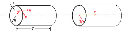
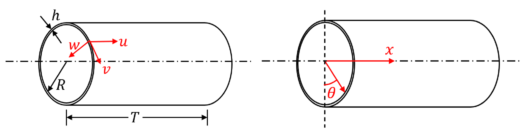
In this study, we proposed to use the shell theory in the tire modeling approach. Figure 1 demonstrates the conventional coordinate system of a cylindrical shell:

Figure 1. Conventional system of a cylindrical shell.

Assume that a circular cylindrical thin shell has radius R, axial length T, thickness d, with $d<<T$. The material is assumed isotropic. For an infinitesimal element on the shell, its displacement along the axial, circumferential, and radial directions are denoted as u, v, and w. Donnell–Mushtari (D-M) shell theory [40] states that the equation for the total strain energy in a cylindrical shell is written as

$$\begin{array}{c}\hfill U_S={\displaystyle \frac{Ed}{2(1-{\nu }^2)}}{\int }_0^{2\pi }{\int }_0^{1}Idsd\theta ,s=x/T\end{array}$$

(5)

$$\begin{array}{cc}\hfill I& ={\left({\displaystyle \frac{\partial u}{\partial s}}+{\displaystyle \frac{\partial v}{\partial \theta }}+w\right)}^2-2(1-\nu )\left[{\displaystyle \frac{\partial u}{\partial s}}\left({\displaystyle \frac{\partial v}{\partial \theta }}+w\right)-{\displaystyle \frac{1}{4}}{\left({\displaystyle \frac{\partial v}{\partial s}}+{\displaystyle \frac{\partial u}{\partial \theta }}\right)}^2\right]\hfill \\ \hfill & +k\left\{{\left({\nabla }^{2}w\right)}^2-2(1-\nu )\left[{\displaystyle \frac{{\partial }^{2}w}{\partial s^2}}{\displaystyle \frac{{\partial }^{2}w}{\partial {\theta }^2}}-{\left({\displaystyle \frac{{\partial }^{2}w}{\partial s\partial \theta }}\right)}^2\right]\right\}\hfill \\ \hfill k& ={\displaystyle \frac{d^2}{12R^2}}\hfill \end{array}$$

(6)

where $U_S$ is the total strain energy, E is the Young’s modulus, $\nu$ is the Poisson’s ratio, I is the integrand to evaluate the strain energy, x is the lateral location along the x-axis, $\theta$ is the angular position, and k is a non-dimensional parameter. Notably, in the field of solid mechanics, the conventional coordinate system is different from the SAE standard reference frame for tires. For solid mechanics, the x-axis is along the central axis of the cylinder, while the SAE standard states that the x-axis is in the longitudinal direction. The derivations above are for isotropic shells. The model can be further developed to include orthotropic properties.

Note that there are various types of shell theories, including but not limited to Love’s, Timoshenko’s, Reissner’s, Vlasov’s, Sanders’, and Flügge’s theories. The equations above are derived based on D-M theories, and they may take different forms if other theories are applied. The commonality among these theories is the assumption that the strain and torsion at an arbitrary point on a thin shell can be measured from the strain and torsion at the mid-surface. The distinctions are the way of measuring deformation from the mid-surface to the outer/inner surface and the way of evaluating the deformation at the mid-surface in the first place.

Equations (5) and (6) give the general form of the strain–displacement relationship in D-M theory, compared with Flügge’s theory as given in Equation (7):

$$\begin{array}{c}\hfill \begin{array}{cc}\hfill e_{\alpha }& ={\displaystyle \frac{1}{1+z/R_{\alpha }}}({ϵ}_{\alpha }+z{\kappa }_{\alpha })\hfill \\ \hfill e_{\beta }& ={\displaystyle \frac{1}{1+z/R_{\beta }}}({ϵ}_{\beta }+z{\kappa }_{\beta })\hfill \\ \hfill {\gamma }_{\alpha \beta }& ={\displaystyle \frac{1}{(1+z/R_{\alpha })(1+z/R_{\beta })}}\left[\left(1-{\displaystyle \frac{z^2}{R_{\alpha }{R}_{\beta }}}\right){ϵ}_{\alpha \beta }+z\left(1+{\displaystyle \frac{z}{2R_{\alpha }}}+{\displaystyle \frac{z}{2R_{\beta }}}\right)\right]\hfill \end{array}\end{array}$$

(7)

where $e_{\alpha }$, $e_{\beta }$ and ${\gamma }_{\alpha \beta }$ denote the strain components at an arbitrary point; z denotes its distance to the mid-surface of the thin shell; and ${ϵ}_{\alpha }$, ${ϵ}_{\beta }$ and ${ϵ}_{\alpha \beta }$ denote the strain components at the mid-surface. It is noticed that Flügge’s theory involves more nonlinear components. The primary reason why D-M theory was chosen for this study was to decrease the complexity of the analytical derivation part of the model, especially for the orthotropic shell part. On the other hand, the majority of the nonlinearity of the tire model comes from the sidewall stiffness, and including more nonlinear terms in the shell stiffness does not lead to a noticeable improvement in the results.

2.4. Energy Method

With the model assumed to be elastic and determinate, Castigliano’s first theorem is applied to derive the forces and deformation equations. The theorem can be considered a rephrase of the principle of stationary potential energy [41]. Notably the model represents a quasi-static loading process, with hysteresis excluded from the scope of this study:

$$\begin{array}{c}\hfill F_i={\displaystyle \frac{\partial U}{\partial u_i}}\end{array}$$

(8)

where $F_i$ denotes the applied force along the ith degree of freedom, U denotes the total strain and potential energy due to elastic deformation, and $u_i$ denotes the displacement of the ith degree of freedom. In this study, the applied deformation ${\mathbf{u}}_{\mathbf{c}}$ is considered to be a given vector to obtain ${\mathbf{F}}_{\mathbf{c}}$, which denotes the reaction force in the contact patch.

3. Model Development

The stiffness of the tire model in the radial direction is due to the inflation pressure, the sidewall, and the tread and belt elements. In the context of this study, the equivalent radial stiffness of the tire is obtained based on the first principles by combining the individual terms for the elements mentioned above. A nonlinear tire model is obtained under the quasi-static, elastic and small to moderate deformation assumptions. The model is then solved using numerical approximations.

3.1. Geometry Setup

The schematic of the tire model is illustrated in Figure 2.

Figure 2. Tire model structure.

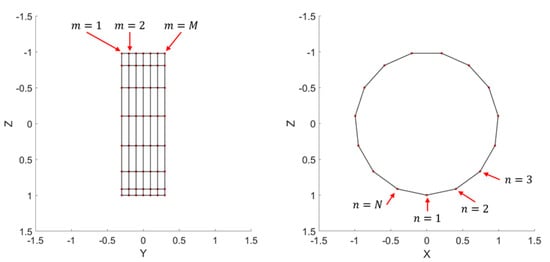
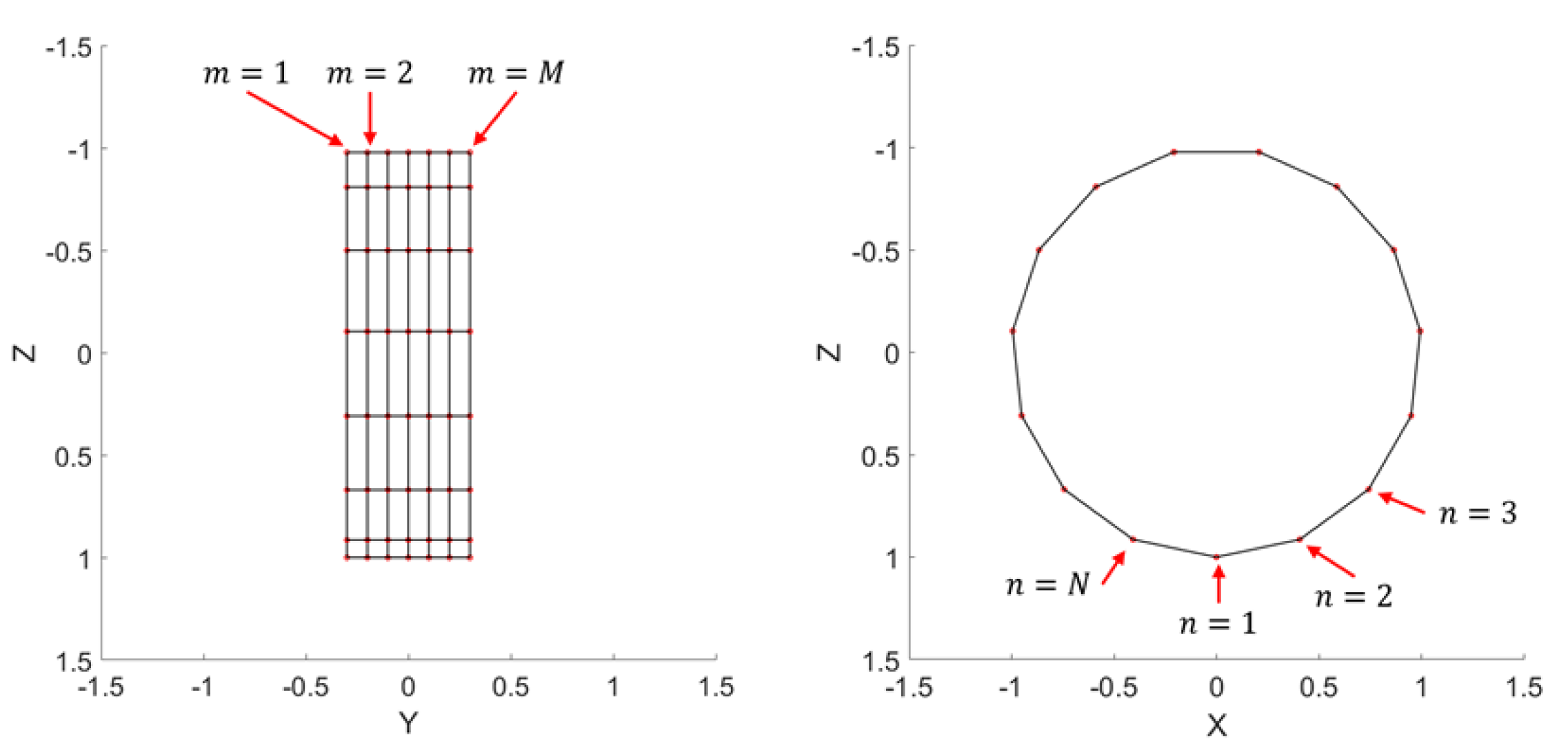
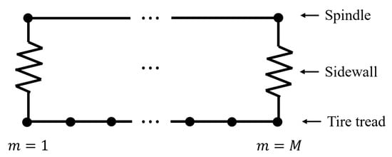
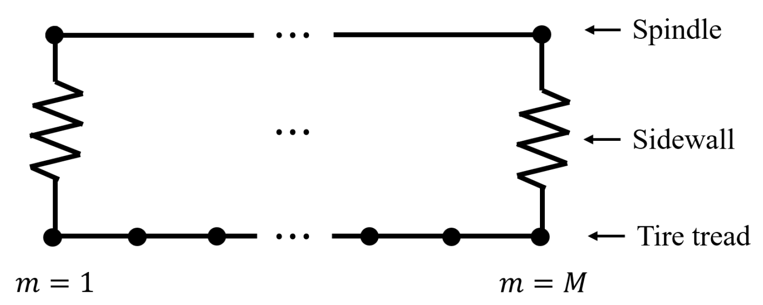
Within the scope of this study, conventional cylindrical system for shell theories introduced in Section 2.3 is used to construct the model, with the origin defined as the center of the unloaded tire. The tread and belt components are modeled as a thin cylindrical shell, supported by a series of radial springs in pairs on the solid rim. The shell is discretized into M lateral layers, each further discretized into N segments in the circumferential direction. Each shell segment represents one degree of freedom of the model and is connected to the rim by radial springs. The springs represent the radial stiffness of the tire. The displacements at the ends of the springs are evaluated to obtain the deformed profile and the spindle force. The discretized shell is shown in Figure 3.

Figure 3. 3D tire model illustrating lateral layers and circumferential nodes.

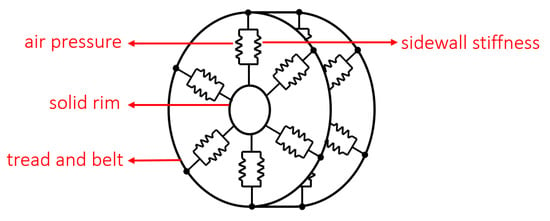
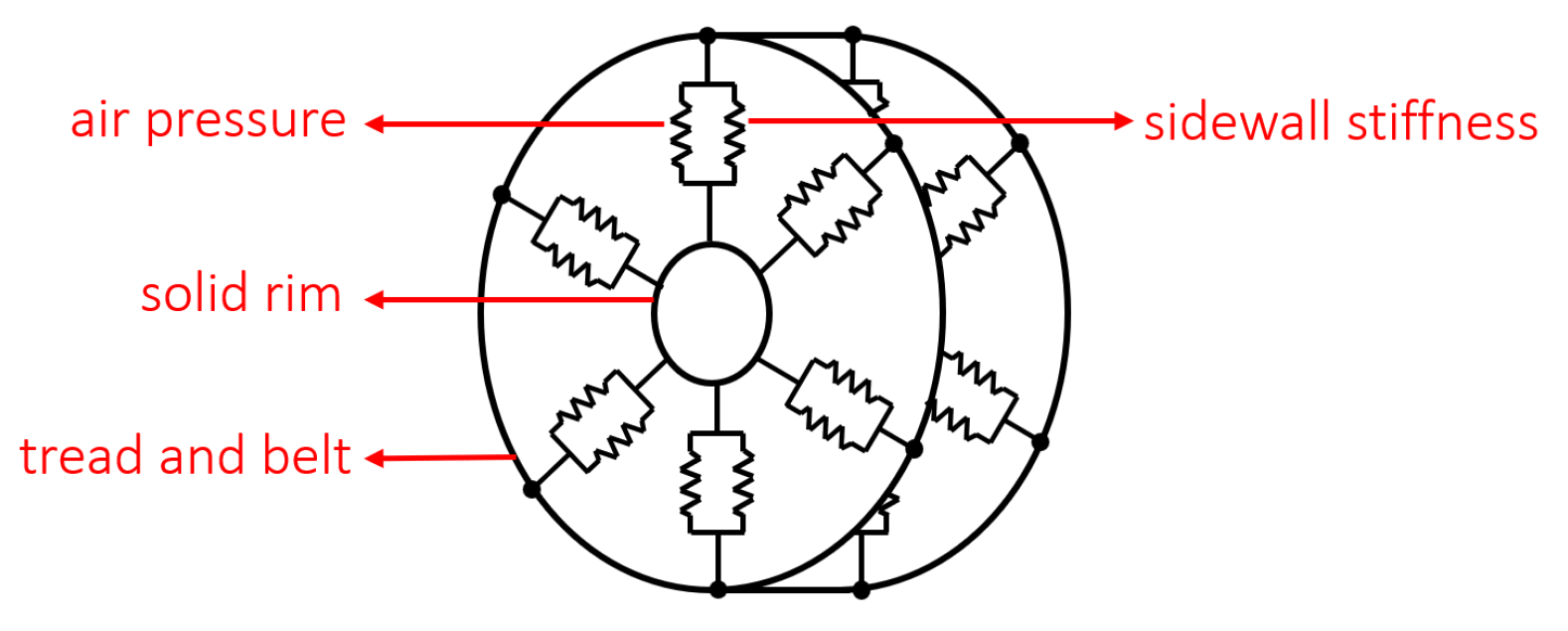
The tire segments are numbered for the sake of constructing the stiffness matrix. It is important to note that the radial stiffness values due to the sidewalls are set to be 0 for intermediate layers of tread and belt segments because the sidewalls are not physically there and the central part of the tire is filled with compressed air, as is shown in Figure 4.

Figure 4. Springs representing the sidewall stiffness.

In other words, the elastic foundation is only applied to part of the model. Each segment has displacements in tangential, lateral and radial directions, denoted as $u_{i,j}$, $v_{i,j}$ and $w_{i,j}$, respectively, with $1\le i\le N$ and $1\le j\le M$. The letters are adopted according to the convention of shell theory. The deformation for the entire model is denoted as a vector $\mathbf{x}$, assembling all displacements on all segments. The radius of the tire is denoted as R, while the lateral thickness is denoted as L. The values of M and N should be chosen in such a way that each tire segment obtains similar lengths in the lateral and circumferential directions to avoid a high aspect ratio.

3.2. Inflation Pressure

The approach employed to incorporate the effect of the inflation pressure is similar to the one used for a 2D tire model [42]. Castigliano’s first theorem is used to develop the stiffness equation using derivatives of the displacement field, and the finite difference scheme provided in Equation (4) is used for numerical approximation.

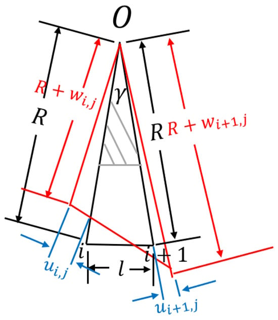
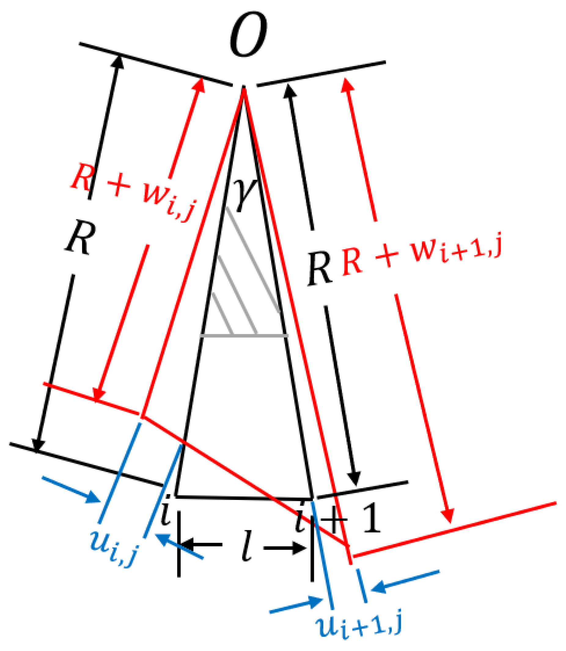
Consider the volume of air between two adjacent shell segments in the same lateral layer, as illustrated in Figure 5. The black lines indicate the undeformed shape of the segment, and the red lines indicate the deformed shape. The contribution of this segment to the overall perimeter is l for the undeformed segment and ${\alpha }_{i}l$ for the deformed segment.

Figure 5. Changes in air volume in a tire segment.

The point O denotes the center of the tire, and R denotes its unloaded radius. For the ${(i,j)}^{th}$ and ${(i+1,j)}^{th}$ segment, $w_{i,j}$ and $w_{i+1,j}$ denote the radial displacement, whereas $u_{i,j}$ and $u_{i+1,j}$ denote the tangential displacement, respectively. $\gamma$ is the angle between two segments, where $\gamma =2\pi /N$. The gray shaded area denotes the solid rim at the center that does not contain air, denoted by $S_{grey}$. The ratio of the tire cross-sectional area divided by the total cross-sectional area of the wheel is defined as $\eta$.

$$\begin{array}{c}\hfill {\displaystyle \frac{R^2\sin \gamma -S_{grey}}{R^2\sin \gamma }}=\eta \end{array}$$

(9)

The work done by the external load to change the volume of the air from $V_1$ to $V_2$ is calculated by Equation (10), with ideal gas and isothermal assumptions:

$$\begin{array}{cc}\hfill U& =-c\ln {\displaystyle \frac{V_2}{V_1}}\hfill \end{array}$$

(10)

where

$$\begin{array}{cc}\hfill V_1& =\eta NT{R}^2\sin \gamma \hfill \\ \hfill V_2& ={\displaystyle \sum _{i=1}^N}{\displaystyle \sum _{j=2}^{M-1}}\left[\left(R+w_{i,j}\right)\left(R+w_{i+1,j}\right)\sin \left(\gamma +{\displaystyle \frac{u_{i+1,j}-u_{i,j}}{R}}\right)\right]\left[{\displaystyle \frac{T}{M-1}}+\left(v_{i,j+1}-v_{i,j}\right)\right]\hfill \\ \hfill & +{\displaystyle \frac{1}{2}}{\displaystyle \sum _{i=1}^N}\left[\left(R+w_{i,1}\right)\left(R+w_{i+1,1}\right)\sin \left(\gamma +{\displaystyle \frac{u_{i+1,1}-u_{i,1}}{R}}\right)\right]\left[{\displaystyle \frac{T}{M-1}}+\left(v_{i,2}-v_{i,1}\right)\right]\hfill \\ \hfill & +{\displaystyle \frac{1}{2}}{\displaystyle \sum _{i=1}^N}\left[\left(R+w_{i,M}\right)\left(R+w_{i+1,M}\right)\sin \left(\gamma +{\displaystyle \frac{u_{i+1,M}-u_{i,M}}{R}}\right)\right]\left[{\displaystyle \frac{T}{M-1}}+\left(v_{i,M}-v_{i,M-1}\right)\right]\hfill \\ \hfill & -(1-\eta )NT{R}^2\sin \gamma \hfill \end{array}$$

(11)

$$\begin{array}{cc}\hfill U& =-c\ln {\displaystyle \frac{V_2}{V_1}}\hfill \\ \hfill & =-c\ln \left\{{\displaystyle \frac{1}{\eta NT{R}^2\sin \gamma }}\right[{\displaystyle \sum _{i=1}^N}{\displaystyle \sum _{j=2}^{M-1}}{A}_{i,j}^{*}+{\displaystyle \frac{1}{2}}{\displaystyle \sum _{i=1}^N}{A}_{i,1}^{*}+{\displaystyle \frac{1}{2}}{\displaystyle \sum _{i=1}^N}{A}_{i,M}^{*}\hfill \\ \hfill & -(1-\eta )NT{R}^2\sin \gamma \left]\right\}\hfill \end{array}$$

(12)

where

$$\begin{array}{cc}\hfill A_{i,j}^{*}& =\left(R+w_{i,j}\right)\left(R+w_{i+1,j}\right)\sin \left(\gamma +\mathrm{\Delta }{u}_{i,j}\right)\left[{\displaystyle \frac{T}{M-1}}+\mathrm{\Delta }{v}_{i,j}\right]\hfill \end{array}$$

(13)

$$\begin{array}{c}\hfill \begin{array}{cc}\hfill \mathrm{\Delta }{u}_{i,j}& ={\displaystyle \frac{u_{i+1,j}-u_{i,j}}{R}}\hfill \\ \hfill \mathrm{\Delta }{v}_{i,j}& =v_{i,j+1}-v_{i,j}\hfill \end{array}\end{array}$$

(14)

The scope of this work includes only moderate deformations; therefore, the terms on the order of ${(w_{i,j}/R)}^2<<1$ are omitted. (The experimental data used in this work are for a tire with a radius of 0.4 m undergoing radial deformation less than 0.1 m, leading to coefficients less than 0.0625, which is significantly smaller than others.) After the high-order terms are dropped, certain terms in Equations (12) and (13) can be simplified as

$$\begin{array}{c}\hfill \begin{array}{cc}\hfill & \left(R+w_{i,j}\right)\left(R+w_{i+1,j}\right)\approx R^2+R\left(w_{i,j}+w_{i+1,j}\right)+w_{i,j}{w}_{i+1,j}\hfill \\ \hfill & \sin \left(\gamma +\mathrm{\Delta }{u}_{i,j}\right)=\sin \gamma \cos \mathrm{\Delta }{u}_{i,j}+\cos \gamma \sin \mathrm{\Delta }{u}_{i,j}\approx \sin \gamma +\mathrm{\Delta }{u}_{i,j}\cos \gamma \hfill \\ \hfill & A_{i,j}^{*}\approx \left[R^2+R\left(w_{i,j}+w_{i+1,j}\right)\right]\left[\sin \gamma +\mathrm{\Delta }{u}_{i,j}\cos \gamma \right]\left[{\displaystyle \frac{T}{M-1}}+\mathrm{\Delta }{v}_{i,j}\right]\hfill \end{array}\end{array}$$

(15)

The contribution of the inflation pressure to the stiffness of the tire as an elastic system is calculated by Castigliano’s first theorem, as given in Equations (16)–(18):

$$\left\{\begin{array}{cc}\hfill {\left(F_{i,j}^{\left(u\right)}\right)}_{gas}& ={\mathrm{\Lambda }}_{i,j}^{\left(u\right)}={\displaystyle \frac{\partial U}{\partial u_{i,j}}}\hfill \\ \hfill {\mathrm{\Lambda }}_{i,j}^{\left(u\right)}& =-{\displaystyle \frac{cRT\cos \gamma }{(M-1)V_2}}{C}_{i,j}^{\left(u\right)}.\hfill \end{array}\right.$$

(16)

$$\left\{\begin{array}{cc}\hfill {\left(F_{i,j}^{\left(v\right)}\right)}_{gas}& ={\mathrm{\Lambda }}_{i,j}^{\left(v\right)}={\displaystyle \frac{\partial U}{\partial v_{i,j}}}\hfill \\ \hfill {\mathrm{\Lambda }}_{i,j}^{\left(v\right)}& =-{\displaystyle \frac{c{R}^2\sin \gamma }{V_2}}{C}_{i,j}^{\left(v\right)}\hfill \end{array}\right.$$

(17)

$$\left\{\begin{array}{cc}\hfill {\left(F_{i,j}^{\left(w\right)}\right)}_{gas}& ={\mathrm{\Lambda }}_{i,j}^{\left(w\right)}={\displaystyle \frac{\partial U}{\partial w_{i,j}}}\hfill \\ \hfill {\mathrm{\Lambda }}_{i,j}^{\left(w\right)}{|}_{1<j<M}& =-{\displaystyle \frac{2cT\sin \gamma }{(M-1)\left[\eta NTR\sin \gamma +\frac{\mathrm{\Delta }{V}_w+\mathrm{\Delta }{V}_u+\mathrm{\Delta }{V}_v}{R}\right]}}\hfill \\ \hfill {\mathrm{\Lambda }}_{i,j}^{\left(w\right)}{|}_{j=1,M}& =-{\displaystyle \frac{cT\sin \gamma }{(M-1)\left[\eta NTR\sin \gamma +\frac{\mathrm{\Delta }{V}_w+\mathrm{\Delta }{V}_u+\mathrm{\Delta }{V}_v}{R}\right]}}\hfill \end{array}\right.$$

(18)

where $\mathrm{\Lambda }$ denotes the contribution of inflation pressure to stiffness. Other terms are defined as follows:

$$\begin{array}{cc}\hfill \mathrm{\Delta }{V}_u& ={\displaystyle \frac{RT\cos \gamma }{M-1}}\left[{\displaystyle \sum _{i=1}^N}{\displaystyle \sum _{j=2}^{M-1}}\left(u_{i+1,j}-u_{i,j}\right)+{\displaystyle \frac{1}{2}}{\displaystyle \sum _{i=1}^N}\left(u_{i+1,1}-u_{i,1}\right)\right.\hfill \\ \hfill & +\left.{\displaystyle \frac{1}{2}}{\displaystyle \sum _{i=1}^N}\left(u_{i+1,M}-u_{i,M}\right)\right]\hfill \\ \hfill \mathrm{\Delta }{V}_v& =R^2\sin \gamma \left[{\displaystyle \sum _{i=1}^N}{\displaystyle \sum _{j=2}^{M-1}}\left(v_{i,j+1}-v_{i,j}\right)+{\displaystyle \frac{1}{2}}{\displaystyle \sum _{i=1}^N}\left(v_{i,2}-v_{i,1}\right)\right.\hfill \\ \hfill & \left.+{\displaystyle \frac{1}{2}}{\displaystyle \sum _{i=1}^N}\left(v_{i,M}-v_{i,M-1}\right)\right]\hfill \\ \hfill \mathrm{\Delta }{V}_w& ={\displaystyle \frac{RT\sin \gamma }{M-1}}\left[2{\displaystyle \sum _{i=1}^N}{\displaystyle \sum _{j=1}^M}{w}_{i,j}-{\displaystyle \sum _{i=1}^N}{w}_{i,1}-{\displaystyle \sum _{i=1}^N}{w}_{i,M}\right]\hfill \\ \hfill V_2& \approx \eta NT{R}^2\sin \gamma +\mathrm{\Delta }{V}_w+\mathrm{\Delta }{V}_u+\mathrm{\Delta }{V}_v\hfill \\ \hfill C_{i,j}^{\left(u\right)}& ={\displaystyle \frac{\partial }{\partial u_{i,j}}}\left[{\displaystyle \sum _{i=1}^N}{\displaystyle \sum _{j=2}^{M-1}}\left(u_{i+1,j}-u_{i,j}\right)+{\displaystyle \frac{1}{2}}{\displaystyle \sum _{i=1}^N}\left(u_{i+1,1}-u_{i,1}\right)\right.\hfill \\ \hfill & \left.+{\displaystyle \frac{1}{2}}{\displaystyle \sum _{i=1}^N}\left(u_{i+1,M}-u_{i,M}\right)\right]\hfill \\ \hfill C_{i,j}^{\left(v\right)}& ={\displaystyle \frac{\partial }{\partial v_{i,j}}}\left[{\displaystyle \sum _{i=1}^N}{\displaystyle \sum _{j=2}^{M-1}}\left(v_{i,j+1}-v_{i,j}\right)+{\displaystyle \frac{1}{2}}{\displaystyle \sum _{i=1}^N}\left(v_{i,2}-v_{i,1}\right)\right.\hfill \\ \hfill & \left.+{\displaystyle \frac{1}{2}}{\displaystyle \sum _{i=1}^N}\left(v_{i,M}-v_{i,M-1}\right)\right]\hfill \end{array}$$

(19)

Furthermore, the inflation pressure causes the tire to expand radially, which is vital for the load-carrying mechanics of a pneumatic tire [43]. The radial expansion is denoted as q in this study. Unlike the 2D model [42], where q is a constant for all degrees of freedom due to symmetry, the 3D model makes the value of $q_{i,j}$ dependent on its subscripts. The reason is that different lateral layers of segments have different radial stiffness values. The side layers that are connected to the spindle by the sidewalls have much higher radial stiffness and thus expand less in the radial direction. The layers in between are bounded by the shell stiffness only. Such difference will later be reflected in the construction of the stiffness matrix.

Notably, the deformation caused by the external load in this study is measured from the inflated state of the tire. When the tire is inflated by a pressure $p_0$ but not loaded yet, it is derived that

$$\begin{array}{cc}\hfill w_{i,j}& =u_{i,j}=0(\mathrm{No}\mathrm{external}\mathrm{loads}\mathrm{are}\mathrm{applied}\mathrm{yet}.)\hfill \end{array}$$

(20)

$$\begin{array}{cc}\hfill F_{i,j}^{\left(w\right)}{|}_{1<j<M}& ={\displaystyle \frac{(-2)p_0\eta \pi R^{2}T}{\eta NR(M-1)}}\hfill \\ \hfill & =(-1)p_0{\displaystyle \frac{2\pi R}{N}}{\displaystyle \frac{T}{M-1}}\hfill \\ \hfill & =-p_{1}dA\hfill \end{array}$$

(21)

$$\begin{array}{cc}\hfill F_{i,j}^{\left(w\right)}{|}_{j=1,M}& ={\displaystyle \frac{1}{2}}{F}_{i,j}^{\left(w\right)}{|}_{1<j<M}\hfill \end{array}$$

(22)

$$\begin{array}{cc}\hfill F_{i,j}^{\left(u\right)}& =F_{i,j}^{\left(v\right)}=0\hfill \end{array}$$

(23)

which is equivalent to the force exerted on one tread element by the inflation pressure.

3.3. Nonlinear Sidewall Stiffness

A discussion regarding the nonlinearity of the sidewall stiffness has been presented in [42]. It is concluded that the stiffness of the sidewall can be written as

$$\begin{array}{c}\hfill F_s^{\left(w\right)}\left(w_s\right)=k_r{w}_s+f_n\left(w_s\right)\end{array}$$

(24)

where $F_s^{\left(w\right)}$ and $w_s$, respectively, denote the tip load and the displacement of the sidewall as a curved elastic component; $k_r$ denotes the linear part of the elasticity; and $f_n$ denotes the nonlinear part, which can be approximated by a power series. In Section 4, the model adopts the equation in the form

$$\begin{array}{c}\hfill F_s^{\left(w\right)}\left(w_s\right)={\alpha }_1{w}_s+{\alpha }_2{w}_s^2+{\alpha }_3{w}_s^3\end{array}$$

while the higher-order terms are omitted. The choice of an order equal to three is also presented in [42], which establishes that a third-order polynomial is sufficient to capture the nonlinear elasticity within the sidewall based on experimental data.

3.4. Tread Stiffness

Shell theory as stated in Equations (5) and (6) is applied to obtain the strain energy in the tread due to deformation. Equation (5) can be rewritten as

$$\begin{array}{c}\hfill U_S={\displaystyle \frac{Ed}{2(1-{\nu }^2)}}{\displaystyle \sum _{i=1}^N}{\displaystyle \sum _{j=1}^M}{I}_{i,j}\mathrm{\Delta }\theta \mathrm{\Delta }y\end{array}$$

(25)

where $I_{i,j}$ is obtained by replacing the derivative terms in Equation (6) with the following finite difference scheme:

$$\begin{array}{c}\hfill \begin{array}{cc}\hfill {\left(w_{yy}\right)}_{i,j}& ={\displaystyle \frac{w_{i,j+1}-2w_{i,j}+w_{i,j-1}}{{\left(\mathrm{\Delta }y\right)}^2}}\hfill \\ \hfill {\left(w_{\theta \theta }\right)}_{i,j}& ={\displaystyle \frac{w_{i+1,j}-2w_{i,j}+w_{i,j+1}}{{\left(\mathrm{\Delta }\theta \right)}^2}}\hfill \\ \hfill {\left(w_{y\theta }\right)}_{i,j}& ={\displaystyle \frac{w_{i+1,j+1}+w_{i-1,j-1}-w_{i+1,j-1}-w_{i-1,j+1}}{4\left(\mathrm{\Delta }y\right)\left(\mathrm{\Delta }\theta \right)}}\hfill \\ \hfill {\left(u_{yy}\right)}_{i,j}& =\dots \hfill \\ \hfill \dots & \end{array}\end{array}$$

(26)

Castigliano’s first theorem is applied to obtain the contribution of the tread stiffness to the force–deformation relationship as

$${\left[\begin{array}{c}{F}_{i,j}^{\left(u\right)}\\ F_{i,j}^{\left(v\right)}\\ F_{i,j}^{\left(w\right)}\end{array}\right]}_{tread}=\left[\begin{array}{c}{\displaystyle \frac{\partial U_S}{\partial u_{i,j}}}\\ {\displaystyle \frac{\partial U_S}{\partial v_{i,j}}}\\ {\displaystyle \frac{\partial U_S}{\partial w_{i,j}}}\end{array}\right]$$

(27)

Equation (28) gives an example of part of the matrix, which is associated with the radial deformation:

$$\begin{array}{cc}\hfill {\left(F_{i,j}^{\left(w\right)}\right)}_{tread}& ={\displaystyle \frac{\partial U_S}{\partial w_{i,j}}}\hfill \\ \hfill & ={\mathbf{e}}_{\mathbf{25}}({\mathbf{K}}_{\mathbf{local}}^{\left(\mathbf{ww}\right)}\circ {\mathbf{w}}_{\mathbf{local}}){\mathbf{e}}_{\mathbf{25}}^{\mathbf{T}}\hfill \end{array}$$

(28)

where ∘ denotes element-wise multiplication; ${\mathbf{e}}_{\mathbf{25}}$ is a row vector that contains 25 ones in the row, i.e., ${\mathbf{e}}_{\mathbf{25}}=[11\cdots 1]$; and

$$\begin{array}{c}\hfill {\mathbf{w}}_{\mathbf{local}}=\left[\begin{array}{ccccc}{w}_{i-2,j-2}& w_{i-2,j-1}& w_{i-2,j}& w_{i-2,j+1}& w_{i-2,j+2}\\ w_{i-1,j-2}& w_{i-1,j-1}& w_{i-1,j}& w_{i-1,j+1}& w_{i-1,j+2}\\ w_{i,j-2}& w_{i,j-1}& w_{i,j}& w_{i,j+1}& w_{i,j+2}\\ w_{i+1,j-2}& w_{i+1,j-1}& w_{i+1,j}& w_{i+1,j+1}& w_{i+1,j+2}\\ w_{i+2,j-2}& w_{i+2,j-1}& w_{i+2,j}& w_{i+2,j+1}& w_{i+2,j+2}\end{array}\right]\end{array}$$

(29)

$$\begin{array}{cc}\hfill {\mathbf{K}}_{\mathbf{local}}^{\left(\mathbf{ww}\right)}& =\left[\begin{array}{ccccc}{k}_1& k_2& k_3& k_2& k_1\\ k_4& k_5& k_6& k_5& k_4\\ k_7& k_8& k_9& k_8& k_7\\ & & & & \\ & & \ast & & \end{array}\right]\hfill \end{array}$$

(30)

$$\begin{array}{c}\hfill \begin{array}{cc}\hfill k_1& ={\displaystyle \frac{E{T}^2{d}^3}{192\mathrm{\Delta }y\mathrm{\Delta }\theta R^2(\nu +1)}}\hfill \\ \hfill k_2& =0\hfill \\ \hfill k_3& =-{\displaystyle \frac{E{d}^3(4{\mathrm{\Delta }y}^2-{\mathrm{\Delta }\theta }^2{T}^2+{\mathrm{\Delta }\theta }^2{T}^2\nu )}{96\mathrm{\Delta }y{\mathrm{\Delta }\theta }^3{R}^2({\nu }^2-1)}}\hfill \\ \hfill k_4& =0\hfill \\ \hfill k_5& =-{\displaystyle \frac{E{T}^2{d}^3\nu }{12\mathrm{\Delta }y\mathrm{\Delta }\theta R^2({\nu }^2-1)}}\hfill \\ \hfill k_6& ={\displaystyle \frac{E{d}^3({\mathrm{\Delta }y}^2+\nu {\mathrm{\Delta }\theta }^2{T}^2)}{6\mathrm{\Delta }y{\mathrm{\Delta }\theta }^3{R}^2({\nu }^2-1)}}\hfill \\ \hfill k_7& =-{\displaystyle \frac{E{T}^2{d}^3({\mathrm{\Delta }y}^2\nu -{\mathrm{\Delta }y}^2+4{\mathrm{\Delta }\theta }^2{T}^2)}{96{\mathrm{\Delta }y}^3\mathrm{\Delta }\theta R^2({\nu }^2-1)}}\hfill \\ \hfill k_8& ={\displaystyle \frac{E{T}^2{d}^3(\nu {\mathrm{\Delta }y}^2+{\mathrm{\Delta }\theta }^2{T}^2)}{6{\mathrm{\Delta }y}^3\mathrm{\Delta }\theta R^2({\nu }^2-1)}}\hfill \\ \hfill k_9& =-{\displaystyle \frac{Ed(24{\mathrm{\Delta }y}^4{\mathrm{\Delta }\theta }^4{R}^2+12{\mathrm{\Delta }y}^4{d}^2+{\mathrm{\Delta }y}^2{\mathrm{\Delta }\theta }^2{T}^2{d}^2+12{\mathrm{\Delta }\theta }^4{T}^4{d}^2)+15{\mathrm{\Delta }y}^2{\mathrm{\Delta }\theta }^{2}E{T}^2{d}^3\nu }{48{\mathrm{\Delta }y}^3{\mathrm{\Delta }\theta }^3{R}^2({\nu }^2-1)}}\hfill \end{array}\end{array}$$

(31)

The ∗ notation denotes that the matrix entries are symmetric about the third row. Note that Equations (28)–(31) only give an example of the local stiffness matrix due to the shell stiffness in the radial direction in a region not adjacent to the sidewalls. The terms associated with the shell stiffness in the lateral and tangential directions are not listed here in full detail because of their length, but they can be derived in a similar pattern.

The shell model can be further improved to obtain orthotropic properties. The stress–strain relationship for an orthotropic shell, where $\alpha$ and $\beta$ denote the two directions along which the material constants are measured, is as follows:

$$\begin{array}{c}\hfill \begin{array}{cc}\hfill {\sigma }_{\alpha }& ={\displaystyle \frac{1}{1-{\nu }_{\alpha }{\nu }_{\beta }}}(E_{\alpha }{e}_{\alpha }+{\nu }_{\alpha }{E}_{\beta }{e}_{\beta })\hfill \\ \hfill {\sigma }_{\beta }& ={\displaystyle \frac{1}{1-{\nu }_{\alpha }{\nu }_{\beta }}}(E_{\beta }{e}_{\beta }+{\nu }_{\beta }{E}_{\alpha }{e}_{\alpha })\hfill \\ \hfill {\tau }_{\alpha \beta }& =G{\gamma }_{\alpha \beta }\hfill \end{array}\end{array}$$

(32)

with the constraint

$$\begin{array}{c}\hfill {\nu }_{\alpha }{E}_{\beta }={\nu }_{\beta }{E}_{\alpha }\end{array}$$

The total strain energy due to elastic deformation is generally calculated as

$$\begin{array}{cc}\hfill U_S& ={\displaystyle \frac{1}{2}}{\int }_V({\sigma }_{\alpha }{e}_{\alpha }+{\sigma }_{\beta }{e}_{\beta }+{\sigma }_{\alpha \beta }{\gamma }_{\alpha \beta })dV\hfill \end{array}$$

(33)

The integrand is denoted as I. After the terms from Equation (32) are substituted, the integrand can be calculated as

$$\begin{array}{c}\hfill \begin{array}{cc}\hfill I& ={\sigma }_{\alpha }{e}_{\alpha }+{\sigma }_{\beta }{e}_{\beta }+{\sigma }_{\alpha \beta }{\gamma }_{\alpha \beta }\hfill \\ \hfill & ={\displaystyle \frac{1}{1-{\nu }_{\alpha }{\nu }_{\beta }}}\left(E_{\alpha }{e}_{\alpha }^2+{\nu }_{\alpha }{E}_{\beta }{e}_{\alpha }{e}_{\beta }+E_{\beta }{e}_{\beta }^2+{\nu }_{\beta }{E}_{\alpha }{e}_{\alpha }{e}_{\beta }\right)+G{\gamma }_{\alpha \beta }^2\hfill \\ \hfill & =A_{11}{\epsilon }_{\theta }^2+A_{22}{\epsilon }_y^2+2A_{12}{\epsilon }_{\theta }{\epsilon }_y+A_{66}{\gamma }_{\theta y}^2\hfill \\ \hfill & +D_{11}{\kappa }_{\theta }^2+D_{22}{\kappa }_y^2+2D_{12}{\kappa }_{\theta }{\kappa }_y+D_{66}{\kappa }_{\theta y}^2\hfill \end{array}\end{array}$$

(34)

where A and D are the membrane and bending stiffness matrices [40]. The local derivatives can then be replaced by the finite difference scheme shown in Equation (4). The stiffness matrix associated with the shell can be calculated, following the same procedure as from Equations (28)–(31). Equation (35) below gives an example of the local stiffness corresponding to the radial direction, in the same form as Equation (31). Other terms of the model are omitted here due to their length.

$$\begin{array}{c}\hfill \begin{array}{cc}\hfill k_1& ={\displaystyle \frac{G{h}^3}{96\mathrm{\Delta }y\mathrm{\Delta }\theta R}}\hfill \\ \hfill k_2& =0\hfill \\ \hfill k_3& =-{\displaystyle \frac{G{h}^3}{48\mathrm{\Delta }y\mathrm{\Delta }\theta R}}-{\displaystyle \frac{\mathrm{\Delta }y{E}_{\beta }{h}^3}{24{\mathrm{\Delta }\theta }^3{R}^3({\nu }_{\alpha }{\nu }_{\beta }-1)}}\hfill \\ \hfill k_4& =0\hfill \\ \hfill k_5& =-{\displaystyle \frac{h^3(E_{\alpha }{\nu }_{\beta }+E_{\beta }{\nu }_{\alpha })}{24\mathrm{\Delta }y\mathrm{\Delta }\theta R({\nu }_{\alpha }{\nu }_{\beta }-1)}}\hfill \\ \hfill k_6& ={\displaystyle \frac{2{\mathrm{\Delta }y}^2{E}_{\beta }{h}^3+{\mathrm{\Delta }\theta }^2{R}^2{h}^3(E_{\alpha }{\nu }_{\beta }+E_{\beta }{\nu }_{\alpha })}{12\mathrm{\Delta }y{\mathrm{\Delta }\theta }^3{R}^3({\nu }_{\alpha }{\nu }_{\beta }-1)}}\hfill \\ \hfill k_7& =-{\displaystyle \frac{G{h}^3}{48\mathrm{\Delta }y\mathrm{\Delta }\theta R}}-{\displaystyle \frac{\mathrm{\Delta }\theta E_{\alpha }R{h}^3}{24{\mathrm{\Delta }y}^3({\nu }_{\alpha }{\nu }_{\beta }-1)}}\hfill \\ \hfill k_8& ={\displaystyle \frac{{\mathrm{\Delta }y}^2{h}^3(E_{\alpha }{\nu }_{\beta }+E_{\beta }{\nu }_{\alpha })+2{\mathrm{\Delta }\theta }^2{E}_{\alpha }{R}^2{h}^3}{12{\mathrm{\Delta }y}^3\mathrm{\Delta }\theta R({\nu }_{\alpha }{\nu }_{\beta }-1)}}\hfill \\ \hfill k_9& =-{\displaystyle \frac{{6\mathrm{\Delta }y}^4{E}_{\beta }{h}^3+{\mathrm{\Delta }\theta }^{2}h({\mathrm{\Delta }y}^{2}G{R}^2{h}^2+4{\mathrm{\Delta }y}^2{E}_{\alpha }{R}^2{h}^2{\nu }_{\beta }+4{\mathrm{\Delta }y}^2{E}_{\beta }{R}^2{h}^2{\nu }_{\alpha }-{\mathrm{\Delta }y}^{2}G{R}^2{h}^2{\nu }_{\alpha }{\nu }_{\beta })}{24{\mathrm{\Delta }y}^3{\mathrm{\Delta }\theta }^3{R}^3({\nu }_{\alpha }{\nu }_{\beta }-1)}}\hfill \\ \hfill & -{\displaystyle \frac{\mathrm{\Delta }\theta h(12E_{\beta }{\mathrm{\Delta }y}^4{R}^2+6E_{\alpha }{R}^4{h}^2)}{24{\mathrm{\Delta }y}^3{R}^3({\nu }_{\alpha }{\nu }_{\beta }-1)}}\hfill \end{array}\end{array}$$

(35)

3.5. Assembling the Forces and Deformation Equations

The deformation along all DoFs of the model is denoted as a column vector assembling the displacements in the tangential, lateral and radial directions:

$$\begin{array}{c}\hfill \mathbf{x}=\left[\begin{array}{c}\mathbf{u}\\ \mathbf{v}\\ \mathbf{w}\end{array}\right],\mathbf{u}=\left[\begin{array}{c}{u}_{1,1}\\ u_{1,2}\\ ⋮\\ u_{2,1}\\ u_{2,2}\\ ⋮\\ u_{N,M}\end{array}\right],\mathbf{v}=\left[\begin{array}{c}{v}_{1,1}\\ v_{1,2}\\ ⋮\\ v_{2,1}\\ v_{2,2}\\ ⋮\\ v_{N,M}\end{array}\right],\mathbf{w}=\left[\begin{array}{c}{w}_{1,1}\\ w_{1,2}\\ ⋮\\ w_{2,1}\\ w_{2,2}\\ ⋮\\ w_{N,M}\end{array}\right]\end{array}$$

(36)

where the indices $(i,j)$ denote the location of the DoF according to the numbering shown in Figure 3.

It has been mentioned in Section 3.2 that the inflation pressure makes the tire expand radially before it is loaded. In practice, the deformation of a tire, w, is always measured from the inflated but unloaded state of the tire. Therefore, the total elastic deformation of the sidewall is the sum of w and q. The expansion due to inflation pressure for all degrees of freedom is denoted as a vector $\mathbf{q}$:

$$\begin{array}{cc}\hfill \mathbf{q}& =\left[\begin{array}{c}{q}_{1,1}\\ q_{1,2}\\ ⋮\\ q_{2,1}\\ q_{2,2}\\ ⋮\\ q_{N,M}\end{array}\right]\hfill \end{array}$$

(37)

where the indices also denote the correspondence to DoFs in Equation (36). The total elastic deformation is therefore written as

$$\begin{array}{c}\hfill \begin{array}{cc}\hfill w_{i,j,total}& =w_{i,j}+q_{i,j}\hfill \\ \hfill {\mathbf{w}}_{\mathbf{total}}& =\mathbf{w}+\mathbf{q}\hfill \end{array}\end{array}$$

(38)

The radial stiffness term contributed by the inflation pressure from Equation (18) can also be written in the same way as Equation (36):

$$\begin{array}{cc}\hfill \mathrm{\Lambda }& =\left[\begin{array}{c}{\mathrm{\Lambda }}_{1,1}^{\left(u\right)}\\ {\mathrm{\Lambda }}_{1,2}^{\left(u\right)}\\ ⋮\\ {\mathrm{\Lambda }}_{1,1}^{\left(v\right)}\\ {\mathrm{\Lambda }}_{1,2}\\ ⋮\\ {\mathrm{\Lambda }}_{N,M}^{\left(w\right)}\end{array}\right]\hfill \end{array}$$

(39)

The vector ${\mathbf{w}}_{\mathbf{total}}$ should be plugged in to calculate the elastic force. By combining the terms associated with inflation pressure in Equation (18), tread stiffness in Equation (31) and sidewall stiffness in Equation (24), the force–deformation relationship is written as

$$\begin{array}{c}\hfill \mathbf{F}=\mathbf{K}(\mathbf{x}+\left[\begin{array}{c}\left\{0\right\}\\ \left\{0\right\}\\ \mathbf{q}\end{array}\right])+\left[\begin{array}{c}\left\{0\right\}\\ \left\{0\right\}\\ f_n(\mathbf{w}+\mathbf{q})\end{array}\right]+\mathrm{\Lambda }\end{array}$$

(40)

The matrix $\mathbf{K}$ denotes the combination of the tread stiffness and the linear part of the sidewall stiffness; $f_n$ denotes the nonlinear part from the sidewall stiffness. The model has a total of $N\times M$ elements. Therefore, the system in Equation (40) consists of $3NM$ rows, each row corresponding to one element. Note that the radial stiffness representing the sidewall stiffness is added only to the rows that correspond to elements on the outermost layers.

3.6. Newton–Raphson Method

The equation relating the tire forces and deformation is written as

$$\begin{array}{c}\hfill \begin{array}{cc}\hfill \left[\begin{array}{c}{\mathbf{F}}_{\mathbf{c}}\\ \mathbf{0}\end{array}\right]& =\left[\begin{array}{cc}{\mathbf{K}}_{\mathbf{cc}}& {\mathbf{K}}_{\mathbf{cu}}\\ {\mathbf{K}}_{\mathbf{uc}}& {\mathbf{K}}_{\mathbf{uu}}\end{array}\right]\left[\begin{array}{c}{\mathbf{x}}_{\mathbf{c}}+{\mathbf{q}}_{\mathbf{c}}\\ {\mathbf{x}}_{\mathbf{u}}+{\mathbf{q}}_{\mathbf{u}}\end{array}\right]+\left[\begin{array}{c}{f}_n({\mathbf{w}}_{\mathbf{c}}+{\mathbf{q}}_{\mathbf{c}})\\ f_n({\mathbf{w}}_{\mathbf{u}}+{\mathbf{q}}_{\mathbf{u}})\end{array}\right]+\left[\begin{array}{c}{\mathbf{\Lambda }}_{\mathbf{c}}\\ {\mathbf{\Lambda }}_{\mathbf{u}}\end{array}\right]\hfill \end{array}\end{array}$$

(41)

where the vectors $\mathbf{x}$, $\mathbf{q}$, and $\mathbf{\Lambda }$ are rearranged such that the entries in the upper parts of the vectors correspond to the DoFs that are constrained (denoted by the subscript c), or, in other words, in the contact patch. The lower parts of the vectors correspond to the DoFs that are unconstrained (denoted by the subscript u), or, in other words, outside of the contact patch. Note that certain terms of ${\mathbf{q}}_{\mathbf{c}}$, ${\mathbf{q}}_{\mathbf{u}}$, and ${\mathbf{f}}_{\mathbf{n}}$ are zero based on their original positions before rearranging. Equation (41) is a form of Equation (40) rewritten to align with Equation (1) in order to apply Guyan’s reduction method [39].

A function is defined as

$$\begin{array}{c}\hfill {\mathbf{F}}_{\mathbf{u}}={\mathbf{K}}_{\mathbf{uc}}({\mathbf{x}}_{\mathbf{c}}+{\mathbf{q}}_{\mathbf{c}})+{\mathbf{k}}_{\mathbf{uu}}({\mathbf{x}}_{\mathbf{u}}+{\mathbf{q}}_{\mathbf{u}})+f_n({\mathbf{x}}_{\mathbf{u}}+{\mathbf{q}}_{\mathbf{u}})+{\mathrm{\Lambda }}_u\end{array}$$

(42)

where the root of ${\mathbf{F}}_{\mathbf{u}}=\mathbf{0}$ is the desired ${\mathbf{x}}_{\mathbf{u}}$ with which the spindle force and the deformation profile are obtained. It is noted in existing studies that a linear tire model does not deviate from the experimental results significantly in terms of spindle force [42]. Hence, the Newton–Raphson method can be applied to approximate the nonlinear solution, with the linear solution as the starting point, as is shown in Equation (43):

$$\begin{array}{c}\hfill \begin{array}{cc}\hfill \mathbf{0}& ={\mathbf{K}}_{\mathbf{uc}}({\mathbf{x}}_{\mathbf{c}}+{\mathbf{q}}_{\mathbf{c}})+{\mathbf{k}}_{\mathbf{uu}}({\mathbf{x}}_{\mathbf{u}}^{\left(\mathbf{0}\right)}+{\mathbf{q}}_{\mathbf{u}})\hfill \\ \hfill \Rightarrow {\mathbf{x}}_{\mathbf{u}}^{\left(\mathbf{0}\right)}& =-{\mathbf{K}}_{\mathbf{uu}}^{-\mathbf{1}}{\mathbf{K}}_{\mathbf{uc}}({\mathbf{x}}_{\mathbf{c}}+{\mathbf{q}}_{\mathbf{c}})-{\mathbf{q}}_{\mathbf{u}},\hfill \\ \hfill {\mathbf{x}}_{\mathbf{u}}^{\left(\mathbf{s}\right)}& ={\mathbf{x}}_{\mathbf{u}}^{(\mathbf{s}-\mathbf{1})}-{\mathbf{J}}^{-\mathbf{1}}{\mathbf{F}}_{\mathbf{u}}\left({\mathbf{x}}_{\mathbf{u}}^{(\mathbf{s}-\mathbf{1})}\right)\hfill \end{array}\end{array}$$

(43)

where the Jacobian of $F_u$ is calculated as

$$\begin{array}{cc}\hfill \mathbf{J}& ={\mathbf{k}}_{\mathbf{uu}}\hfill \\ \hfill & +diag\left(\left[\begin{array}{ccccc}{f}_n^{\prime }(x_1^{(s-1)}+q)& f_n^{\prime }(x_2^{(s-1)}+q)& f_n^{\prime }(x_3^{(s-1)}+q)& \dots & f_n^{\prime }(x_N^{(s-1)}+q)\end{array}\right]\right)\hfill \\ \hfill & +\mathrm{\Gamma }\hfill \end{array}$$

(44)

where $x_k^{(s-1)}$ denotes the xth entry in the column vector ${\mathbf{x}}_{\mathbf{u}}^{(\mathbf{s}-\mathbf{1})}$. The last term is a square matrix of the same size as ${\mathbf{K}}_{\mathbf{uu}}$. Its entries are calculated as follows:

$$\begin{array}{c}\hfill \mathrm{\Gamma }={\displaystyle \frac{c}{V_2{\left(x\right)}^2}}\left[\begin{array}{ccc}0& 0& 0\\ 0& 0& 0\\ 0& 0& b_w{b}_w^{\mathrm{T}}\end{array}\right]\end{array}$$

(45)

where c is the ideal gas constant, $V_2\left(x\right)$ is the total air volume after the deformation is applied in Equation (19), and

$${\left(b_w\right)}_{i,j}={\displaystyle \frac{RT\sin \gamma }{M-1}}\left\{\begin{array}{cc}1,\hfill & j=1\mathrm{or}j=M,\hfill \\ 2,\hfill & 1<j<M\hfill \end{array}\right.$$

(46)

For the proposed model, the convergence criterion can be set to the maximum element-wise change in the displacement vector, e.g., the iterative process stops if the maximum element-wise change is less than 0.01 mm.

4. Experimental Model Calibration and Simulation Results

The tire model involves a set of parameters, including Young’s modulus E, inflation pressure $p_0$, shell thickness d, Poisson’s ratio $\nu$, and the set of coefficients $\alpha$ that define the nonlinearity in sidewall stiffness. Note that the tire consists of a complicated multilayer structure, and all of these variables are essentially “equivalent” material properties. In other words, the multiple materials of which the tire is made are lumped together and treated as composite materials. This is a common approach for empirical, semi-empirical, and analytical tire models that reduce the numbers of unknowns and equations. The accuracy of the model is achieved by deliberately developing the model so that it reflects tire physics and mechanics despite the simplifications. FEM researchers, such as Chae [13] and Fevers [11], proposed detailed models segmenting the tire into multiple layers, but there are still neglected components or structures.

The rest of this section presents the calibration of the model, followed by comparisons between the experimental data and simulation data.

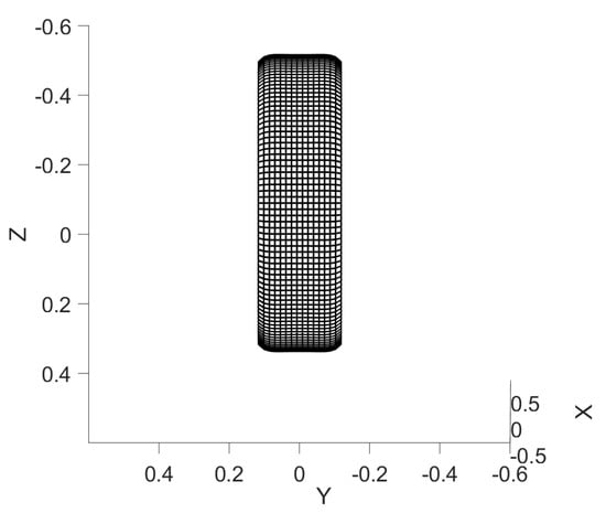
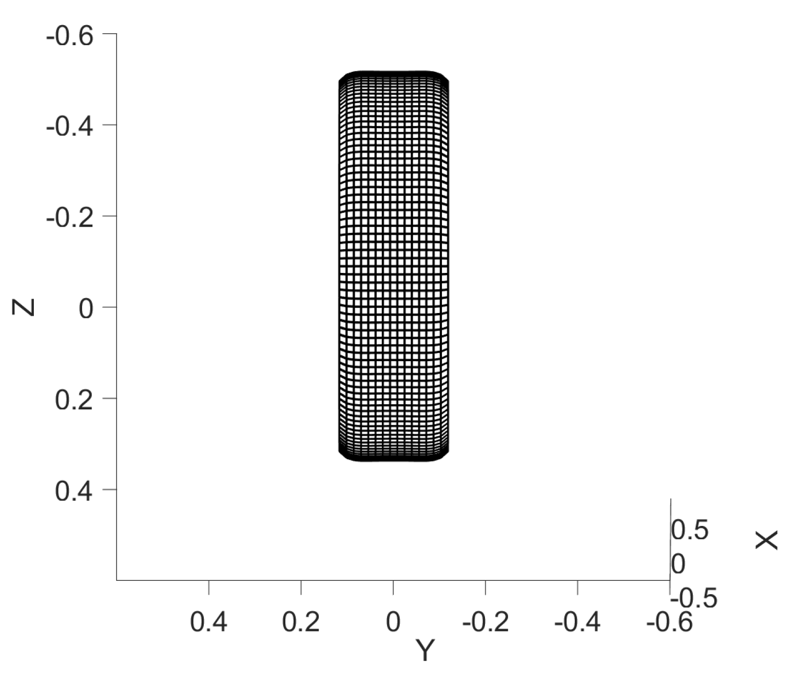
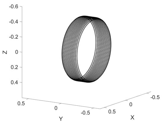
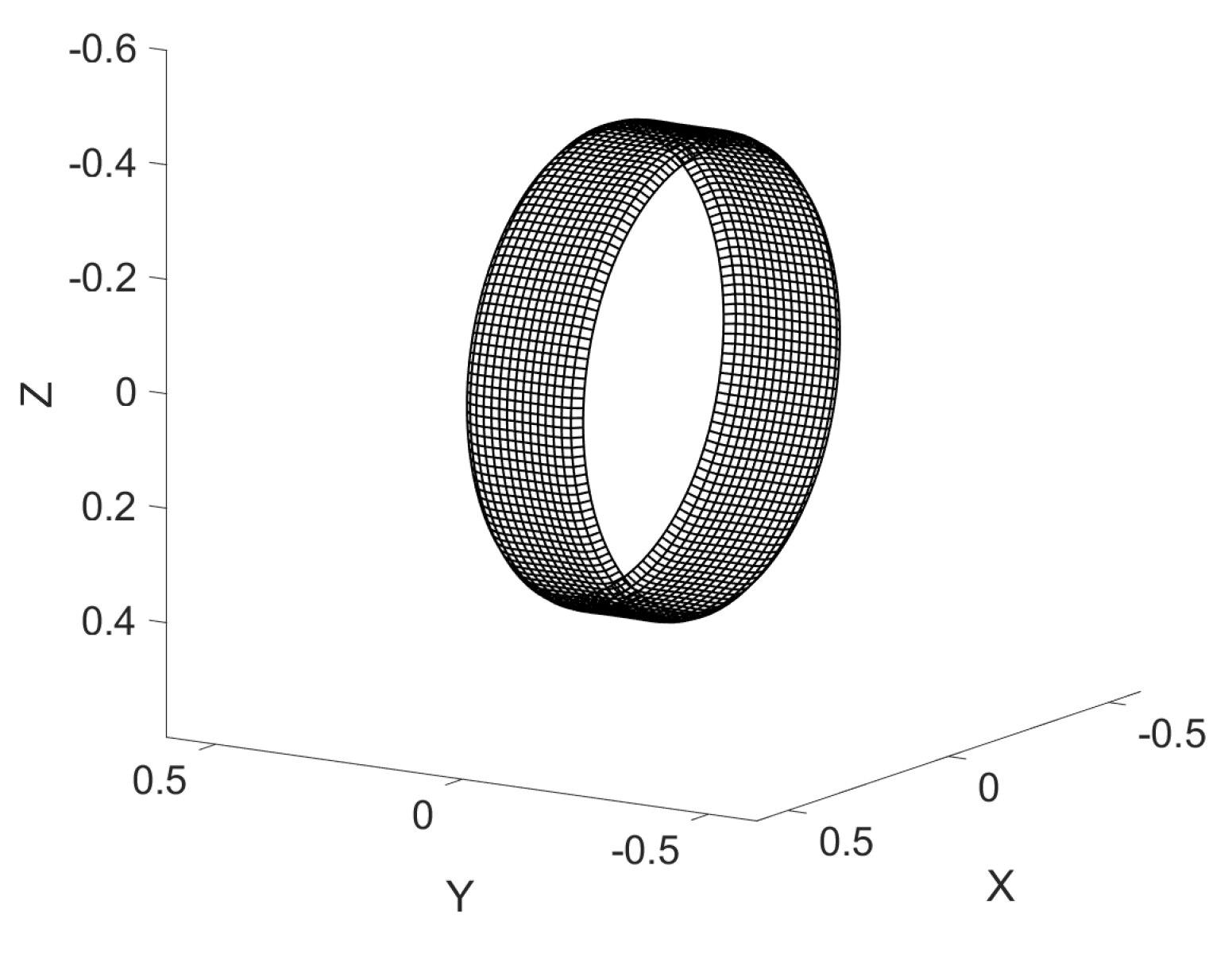
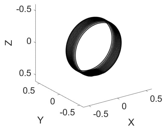
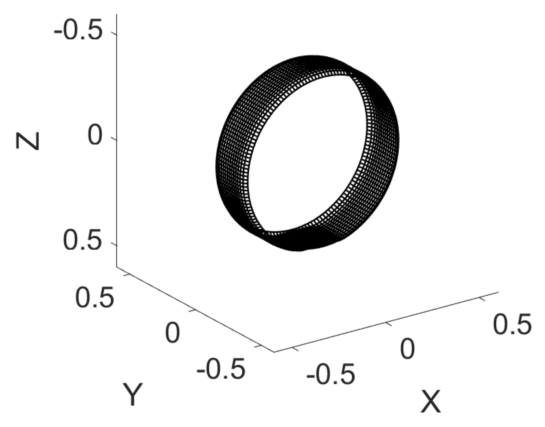
Figure 6, Figure 7 and Figure 8 showcase the 3D tire model, inflated and loaded by a flat plate. Note from Figure 6 that the connection between the sidewall and the tread is a curved shape. This is because the radial springs that represent the sidewall stiffness are only added to the side layers, while the intermediate layers are bounded only by the shell’s stiffness.

Figure 6. Inflated 3D tire model.

Figure 7. Inflated 3D tire model.

Figure 8. Tire loaded by a flat plate.

4.1. Calibration

The experimental data consist of two sets. One was provided by Professor Schalk Els from the University of Pretoria to the Vehicle Terrain Performance Lab at Virginia Tech. The tire tested was the Continental Conti-Trac AT238/85 R16. The tire was mounted to a rigid spindle, and a loading machine slowly pressed a flat plate and cleats of different sizes onto the tire in repeated quasi-static loading processes. Displacement and force transducers were integrated with the loading machine to measure radial deformation and spindle force. This dataset is used to validate the model in terms of predicting normal force.

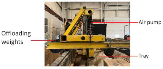
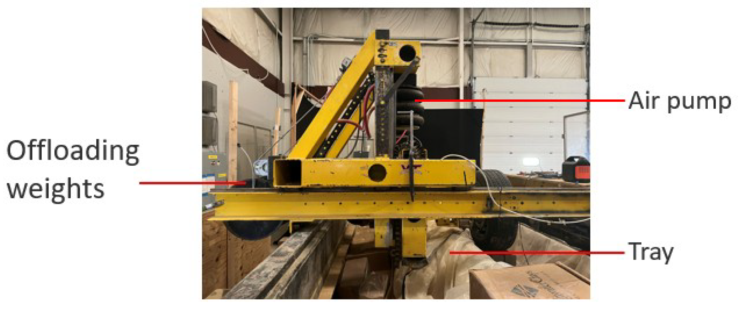
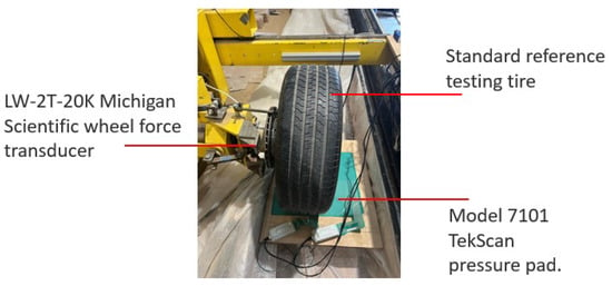
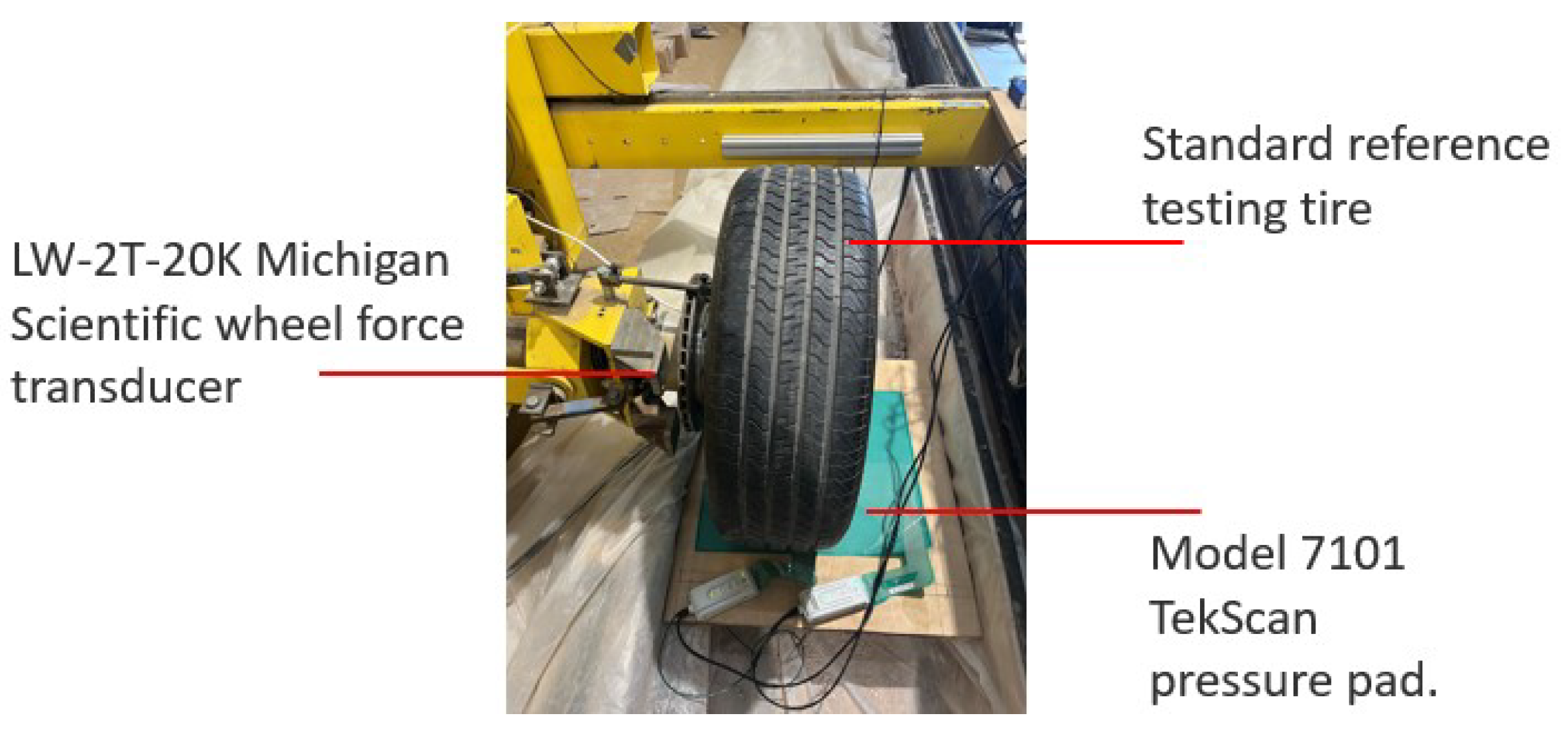
The other set was obtained in the Terramechanics, Multibody and Vehicle Systems Laboratory (TMVS) at Virginia Tech. A Michelin P225/60 R16 standard reference test tire (SRTT) was mounted on a Michigan Scientific LW-2T-20K wheel force transducer installed on the loading machine. A Bosch GLM 15 laser measure recorded the displacement, and a TekScan Model 7101 pressure pad placed between the tire and the rigid surface measured the pressure distribution. The laser measure has a typical measurement accuracy of ±3.0 mm, a display resolution of 1 mm, and a measurement range of 0.15–15 m. The pressure pad has a sensel pitch of 5.1 mm, with a spatial resolution of 3.9 sensels per square centimeter. Tekscan reports linearity and repeatability of less than $\pm 3\%$ and $\pm 3.5\%$, respectively. This dataset is used to verify the ability of the model to predict normal pressure distribution over the contact patch. The tire was pressed against the pressure pad five times under each loading condition for repeatability. The experimental setup is shown in Figure 9 and Figure 10.

Figure 9. Experimental set up in the TMVS lab.

Figure 10. Experimental set up in the TMVS lab.

An optimization process with the interior-point algorithm is adopted to obtain the lumped parameters. The objective is to minimize the squared sum of the differences between simulated spindle force and experimental spindle force.

4.2. Isotropic Shell Tire Model

The model is first used to predict the spindle force. The dataset of the AT238/85 R16 tire is used, and the model is calibrated using the data from both the flat plate test and the 51 mm cleat test. The tire is divided into 16 lateral layers, each discretized into 150 segments in the circumferential direction. The following parameters are identified after calibration:

$$\begin{array}{c}\hfill \begin{array}{cc}\hfill E& =2.722\times {10}^5\hfill \\ \hfill p_0& =5500\hfill \\ \hfill h& =0.0614\hfill \\ \hfill vs.& =0.05\hfill \\ \hfill {\alpha }_1& =8.65\times {10}^3\hfill \\ \hfill {\alpha }_2& =6.464\times {10}^4\hfill \\ \hfill {\alpha }_3& =9.01\times {10}^4\hfill \end{array}\end{array}$$

(47)

The constraints applied to the parameters are that the values of A, B, q should all be greater than 0 and that ${\alpha }_{1}u+{\alpha }_2{u}^2+{\alpha }_3{u}^3\le 0$ for all $-0.1\le u\le 0$ to comply with the physical boundaries associated with the parameters.

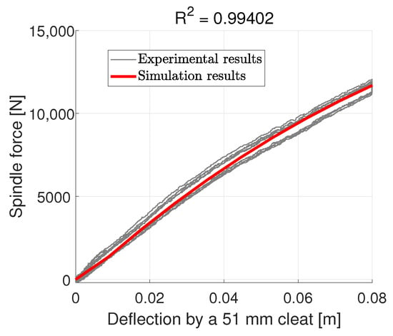
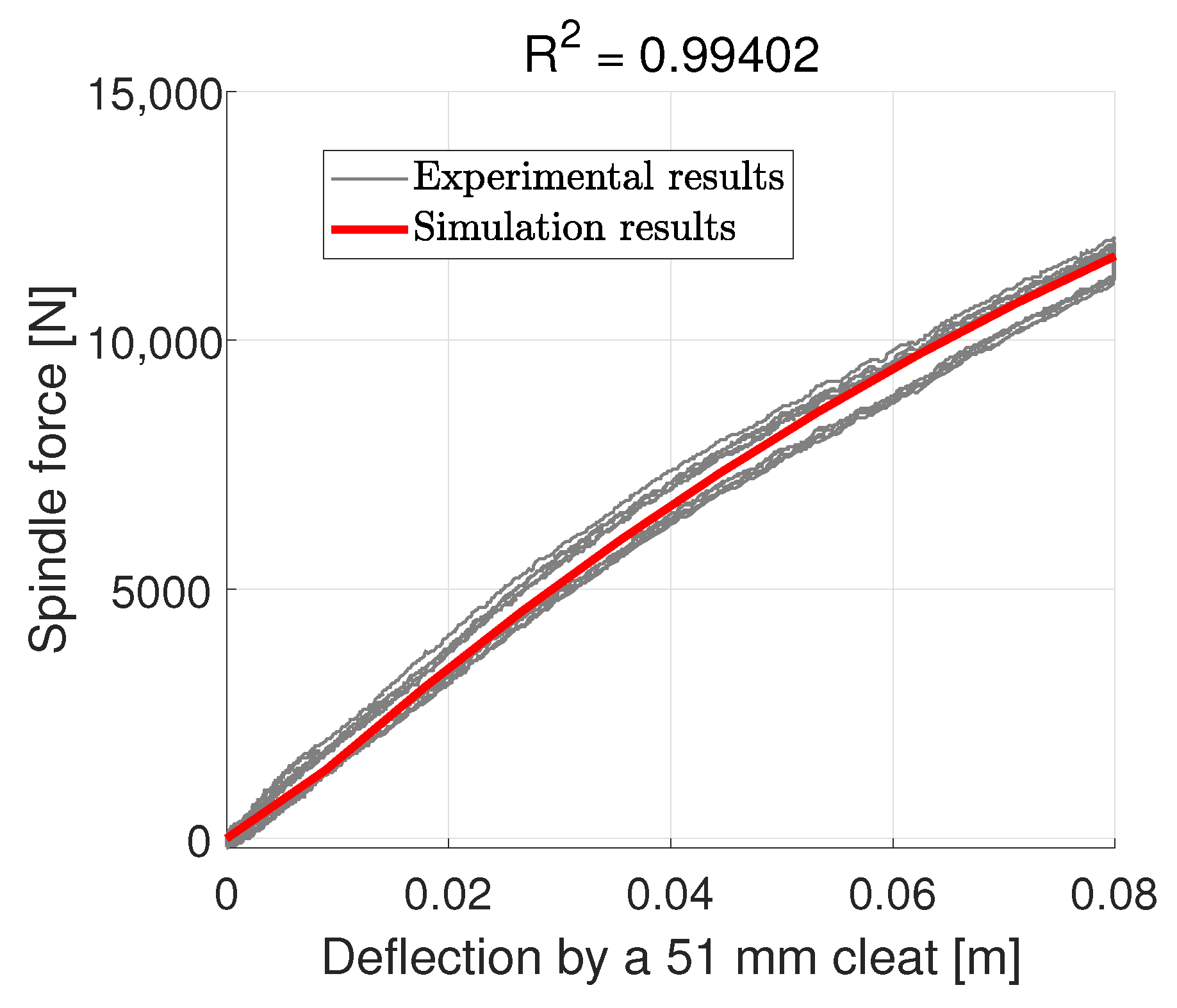
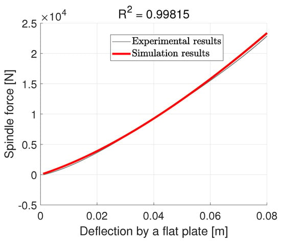
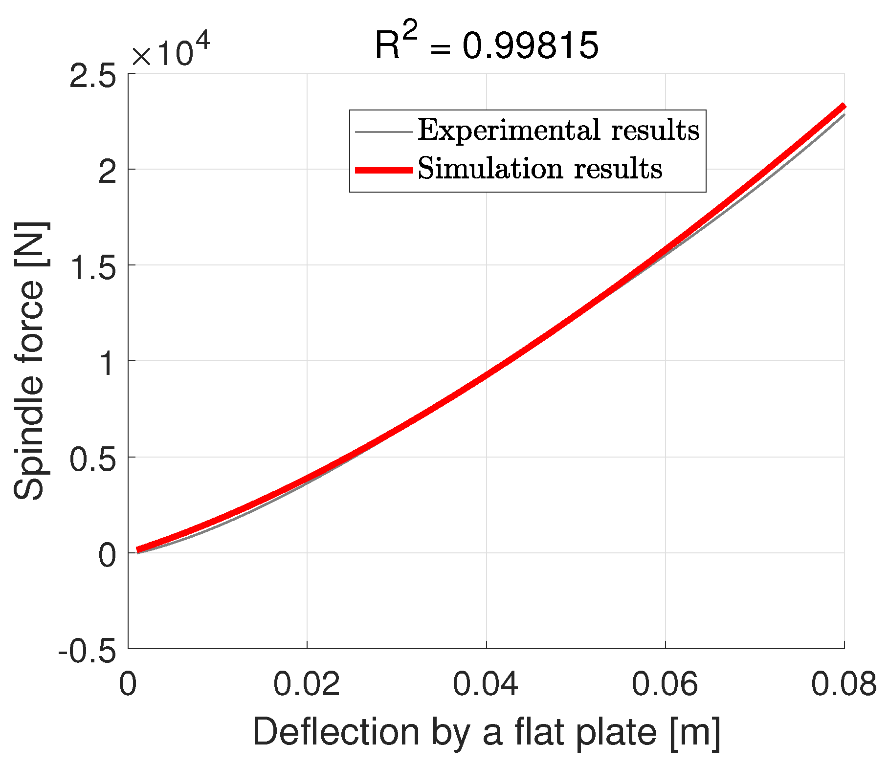
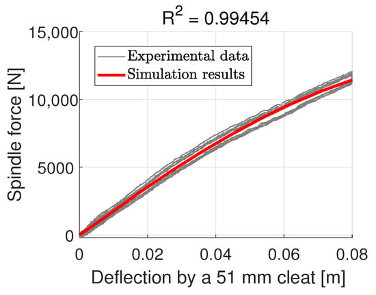
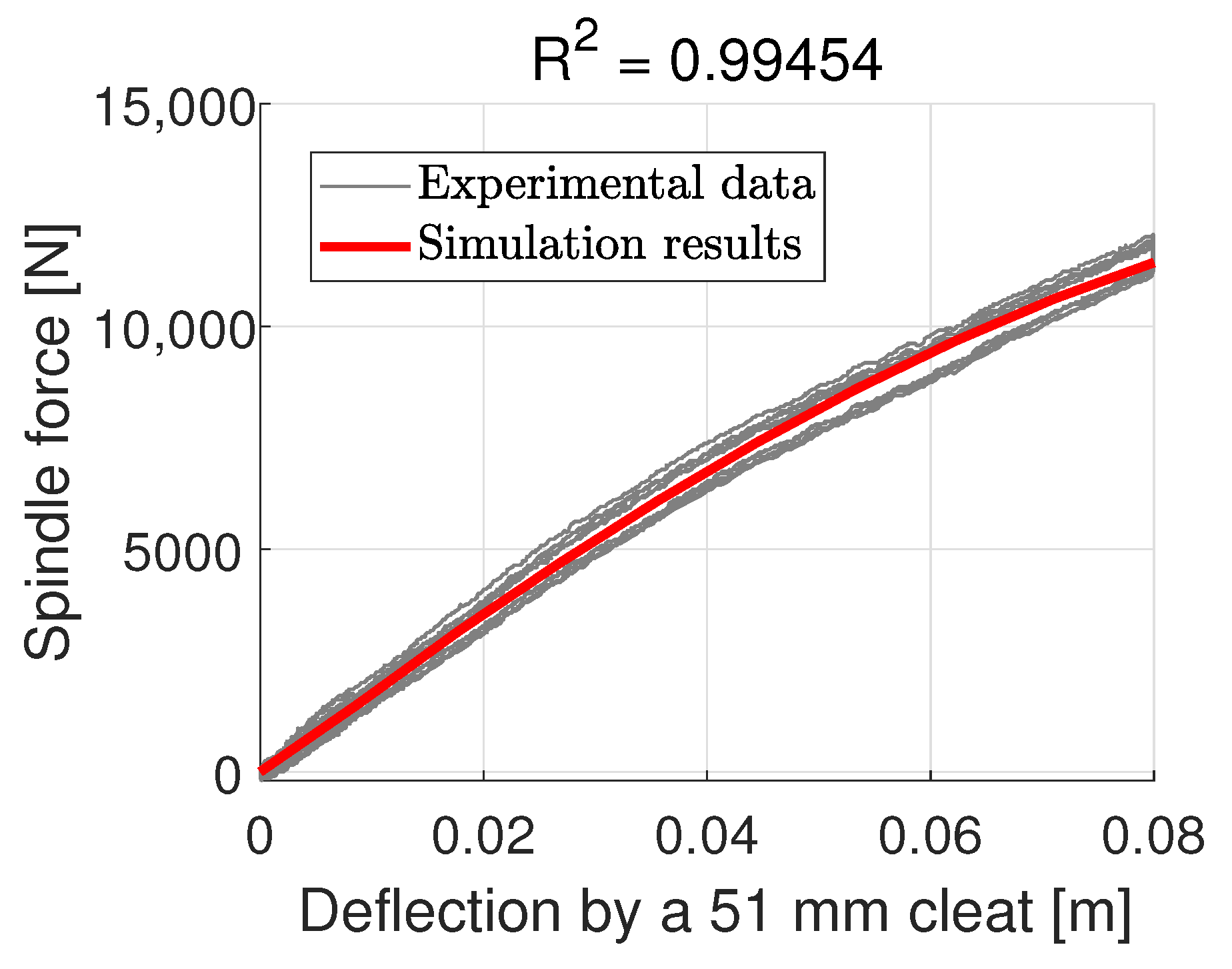
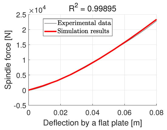
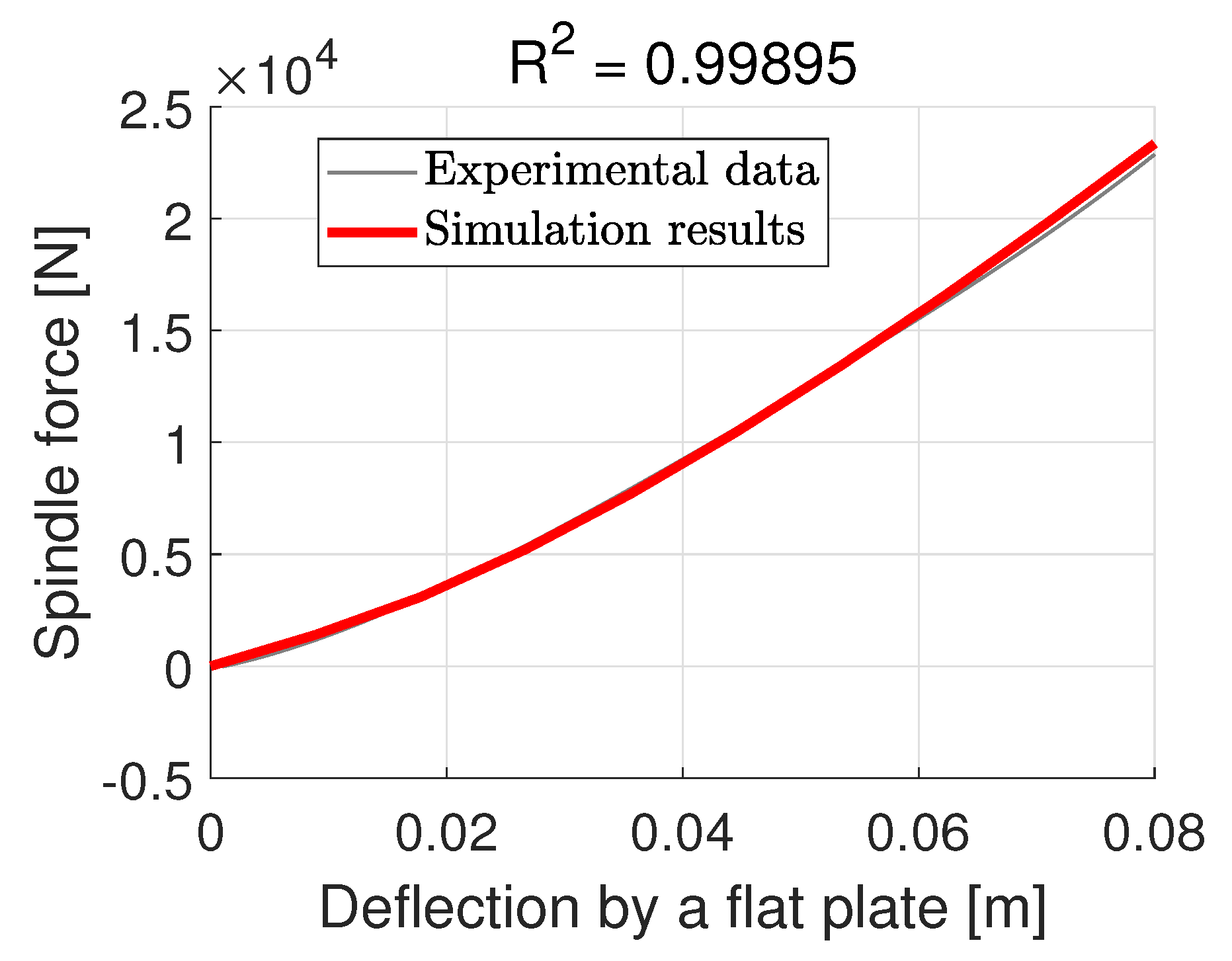
It is shown in Figure 11 and Figure 12 that the model can be calibrated to align with the experimental data, with some minor errors in the case of a flat plate test. The RMSE of the 51 mm cleat calibration is 351.38 N, while that of the flat-plate calibration is 292.85 N. One noticeable issue is that the simulated curve for a flat-plate test shows a tendency to further deviate from the experimental data should the deformation be increased over 0.08 m.

Figure 11. Calibration results with the isotropic shell model.

Figure 12. Calibration results with the isotropic shell model.

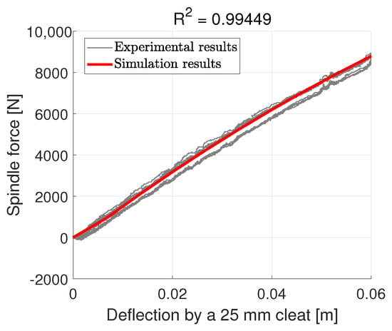
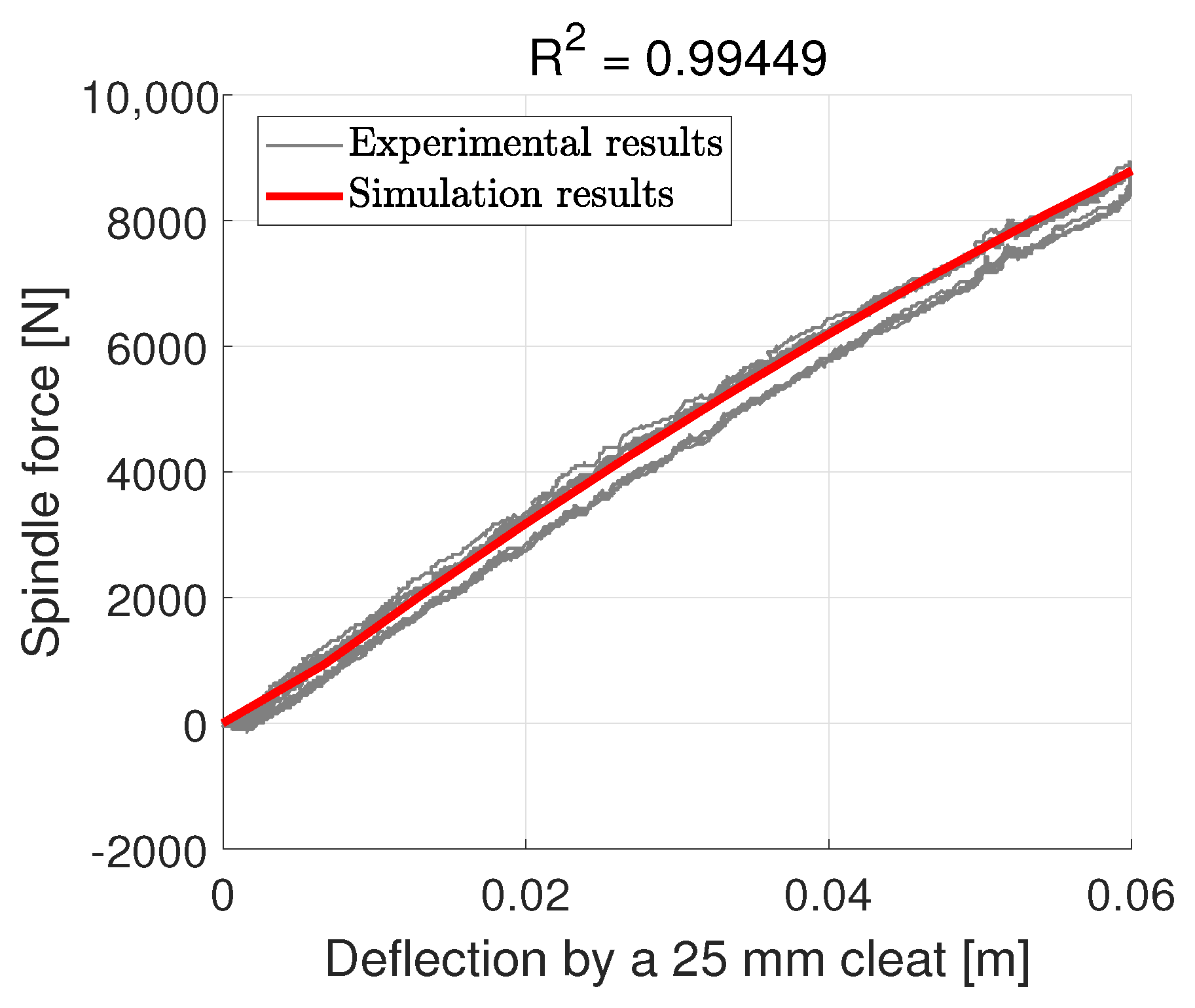
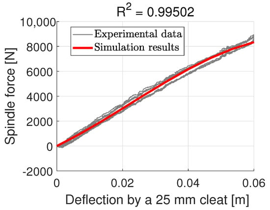
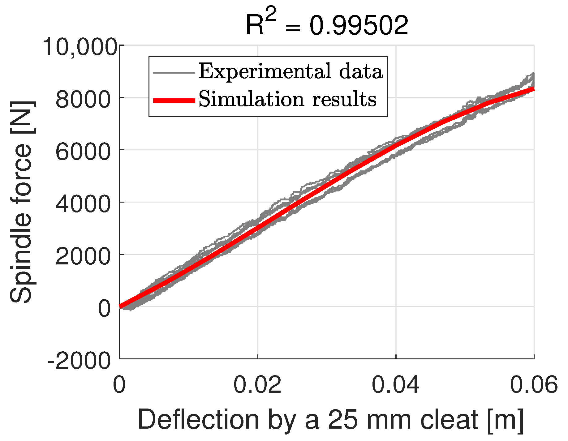
The same set of parameters is then used to predict the spindle force when the tire is loaded by cleats of different sizes. First, consider the results of the cleat test for cleats that are smaller than the 51 mm cleat used for parameter identification. The 25 mm cleat results are shown in Figure 13. The model slightly overestimates the experimental data with an $R^2$ value greater than 0.99, with the RMSE equals 251.52 N.

Figure 13. Spindle force prediction for a 25 mm cleat with the isotropic shell model.

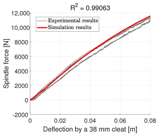
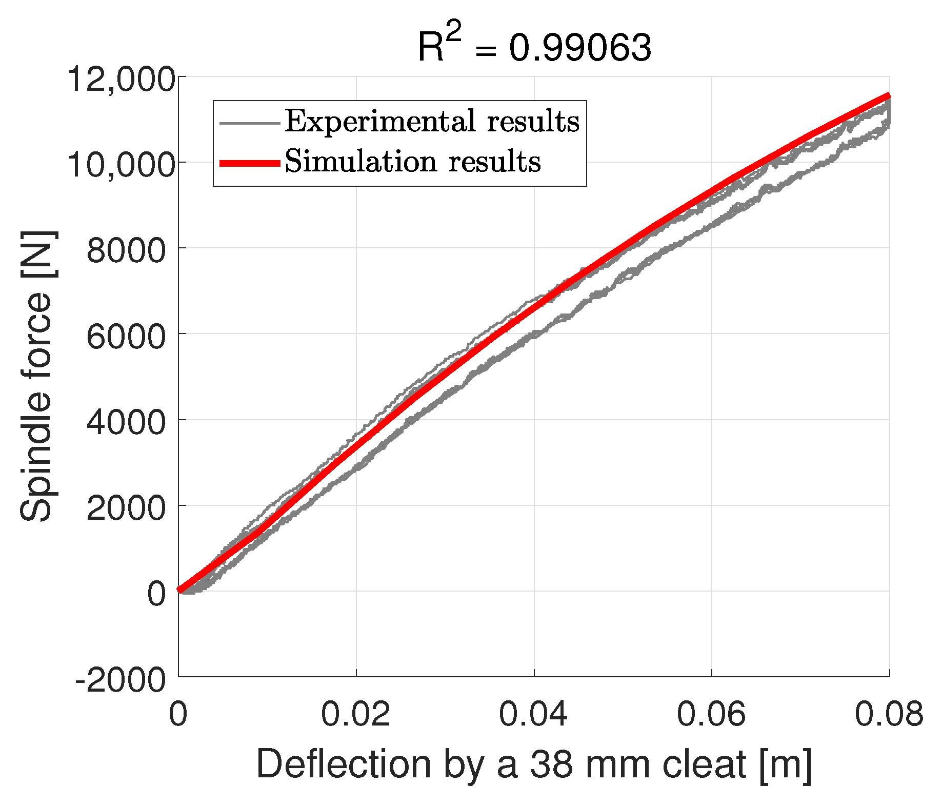
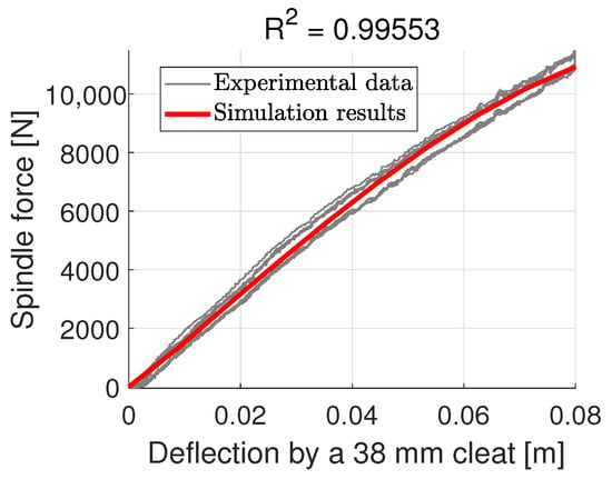
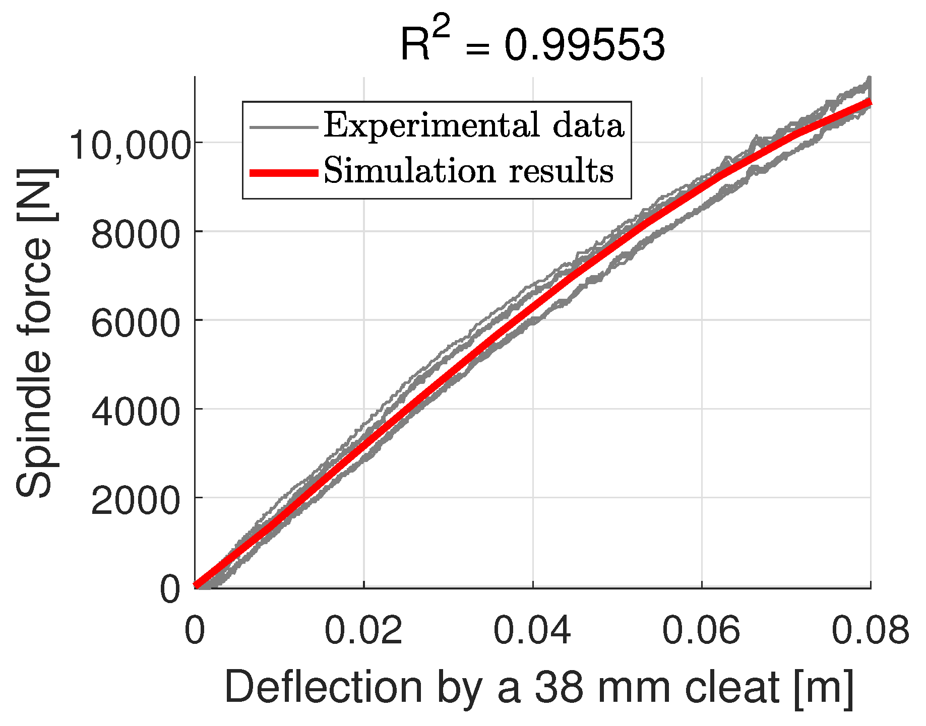
Compared to the 25 mm cleat test, the results of the 38 mm cleat test overestimate the spindle force relative to the experimental data, as shown in Figure 14. The RMSE is 394.27 N.

Figure 14. Spindle force prediction for a 38 mm cleat with the isotropic shell model.

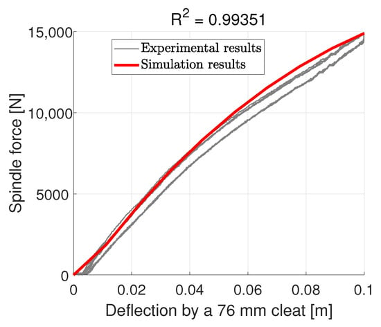
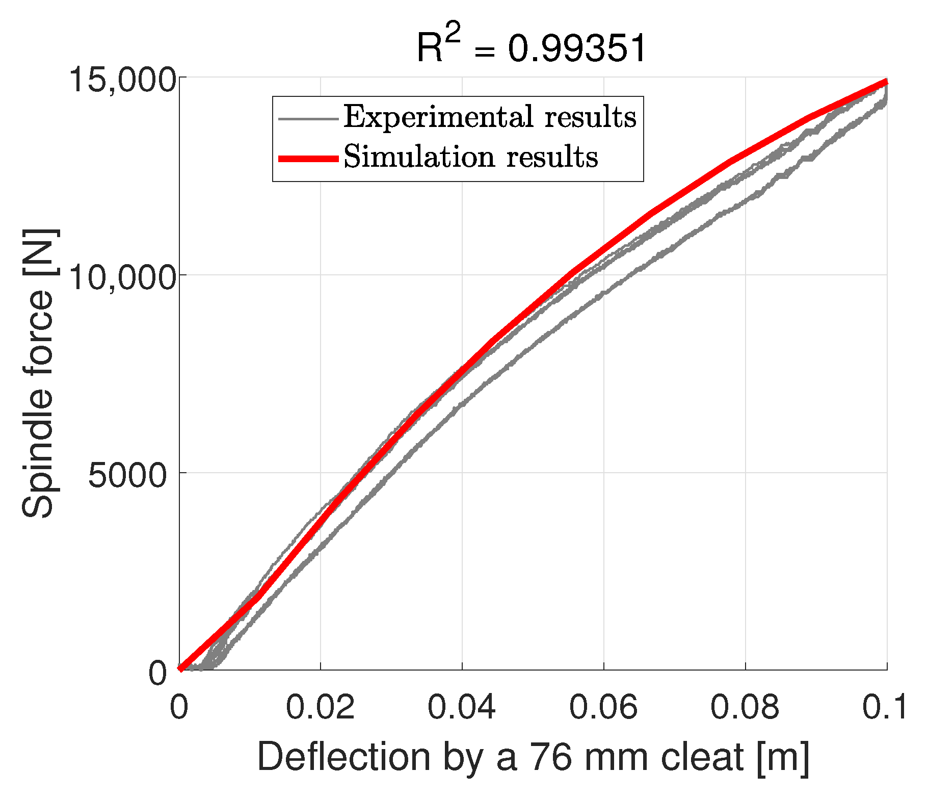
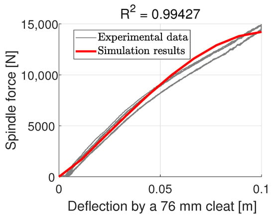
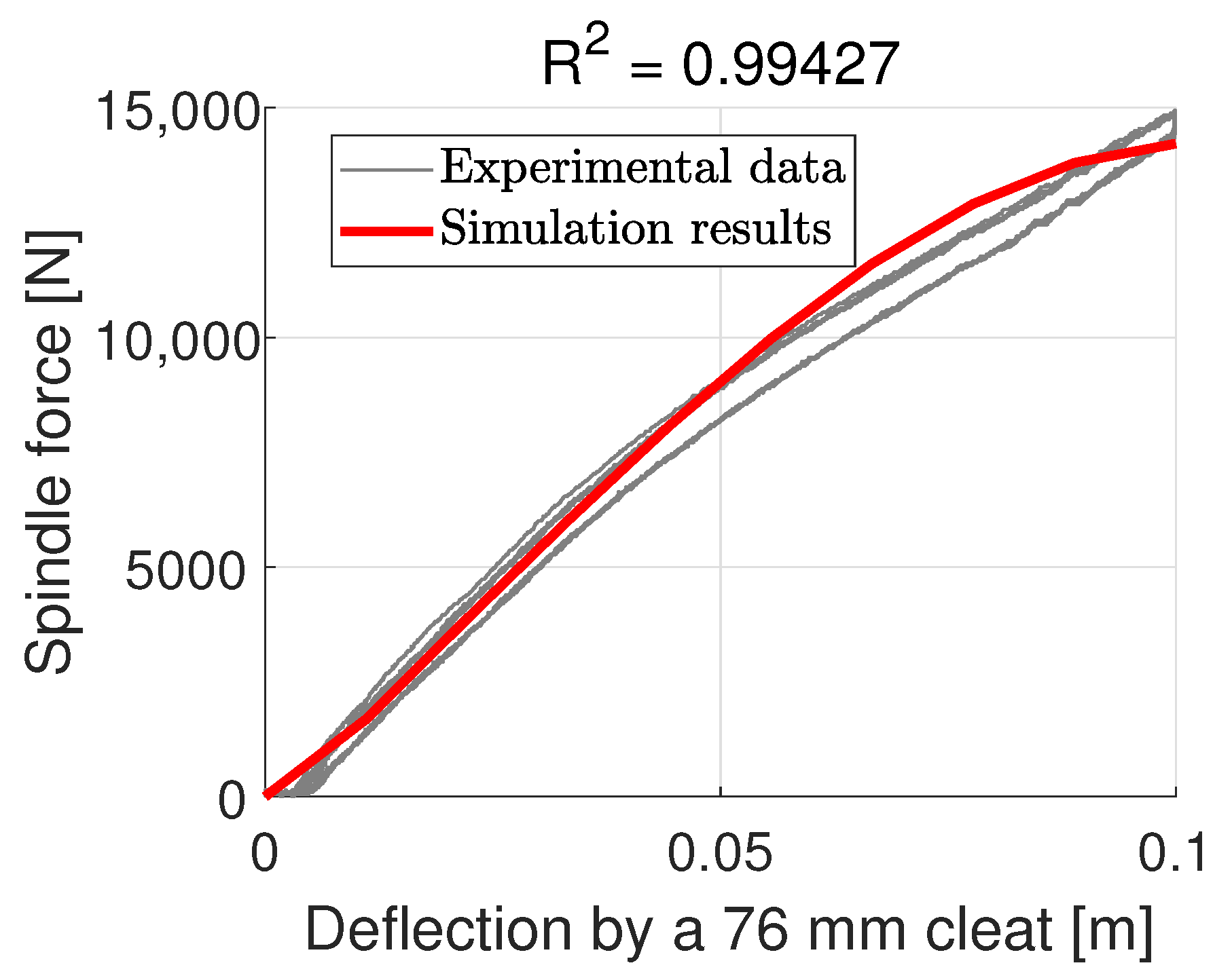
A similar pattern is shown for the 76 mm cleat test but the model converges back at the end with an RMSE of 609.55 N, as shown in Figure 15.

Figure 15. Spindle force prediction for a 76 mm cleat with the isotropic shell model.

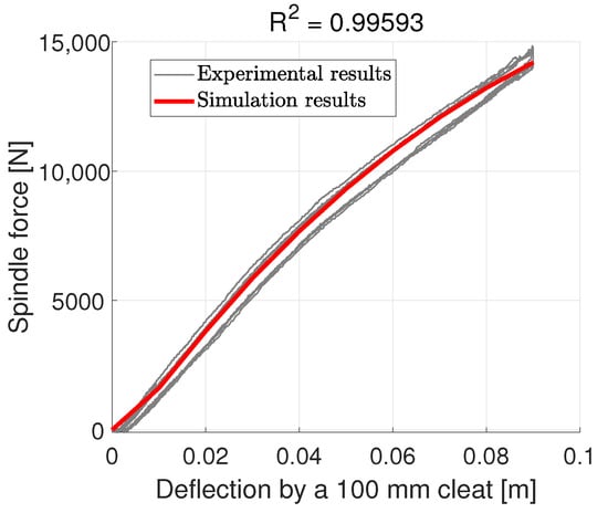
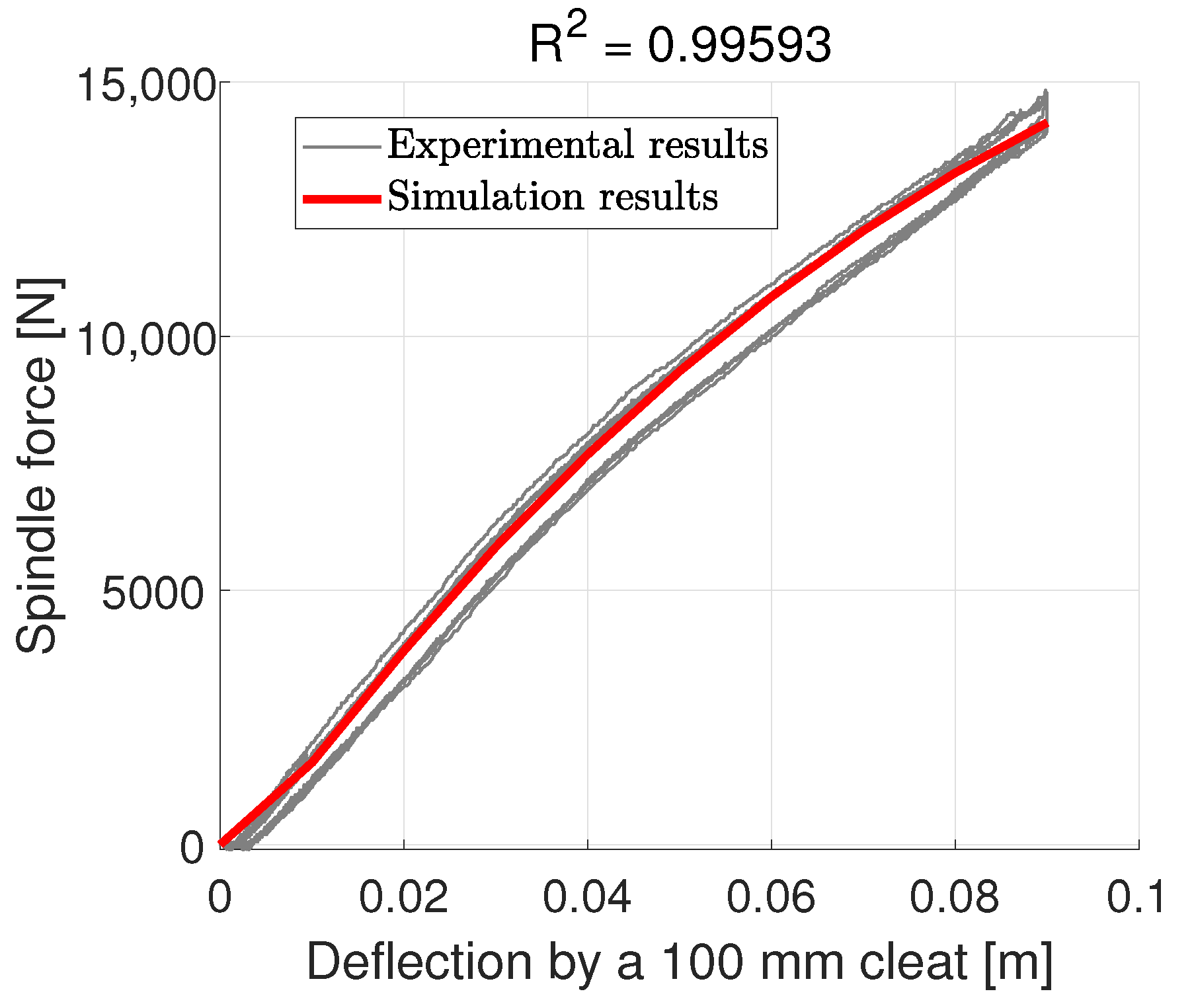
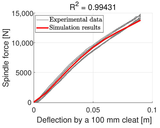
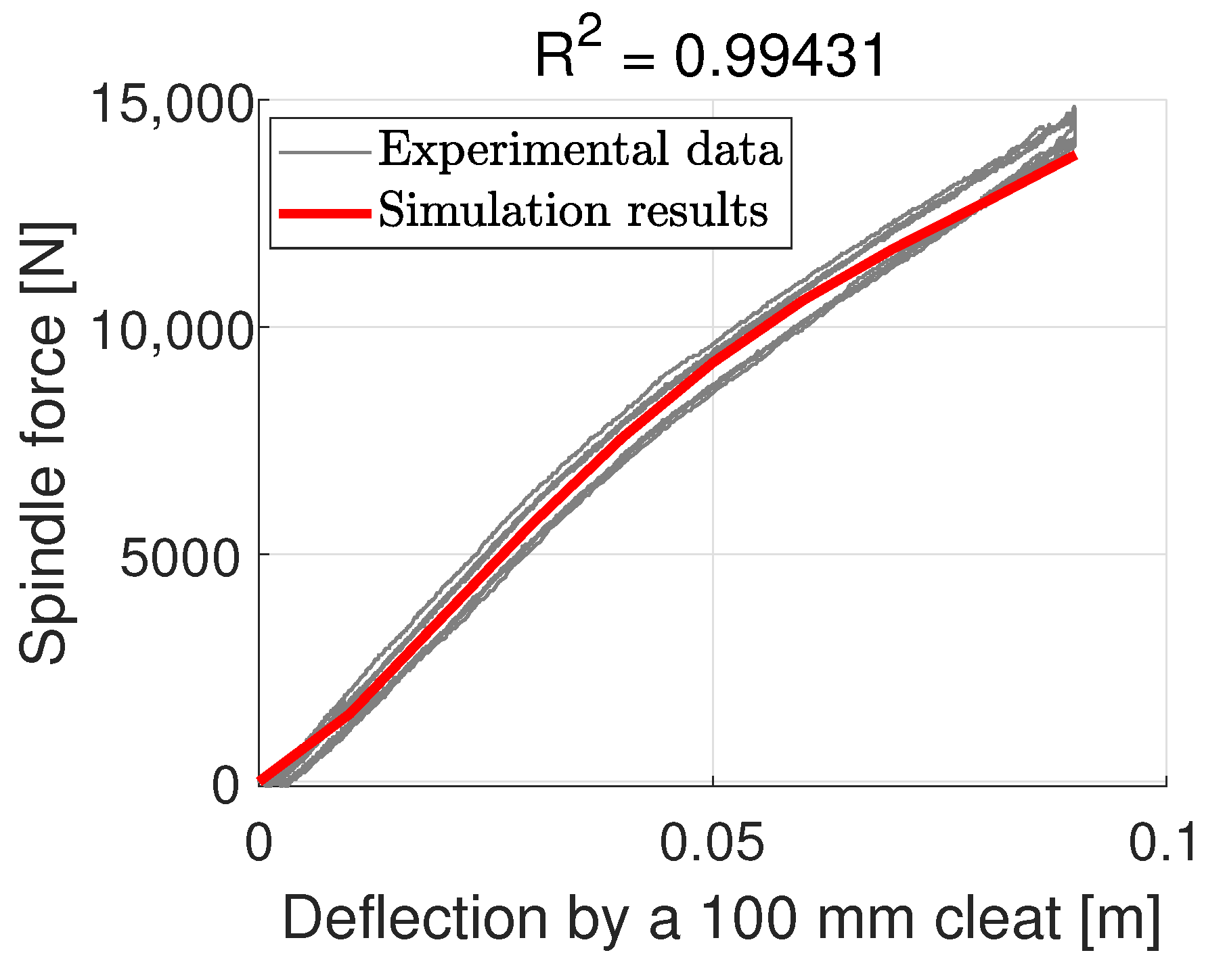
The cases of the 38 mm cleat and the 76 mm cleat both give coefficients of determination greater than 0.98. The prediction for the 100 mm cleat demonstrates a similar pattern but slightly underestimates the spindle force for deformation close to 100 mm, as is shown in Figure 16. The RMSE of this dataset is 385.78 N.

Figure 16. Spindle force prediction for a 100 mm cleat with the isotropic shell model.

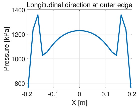
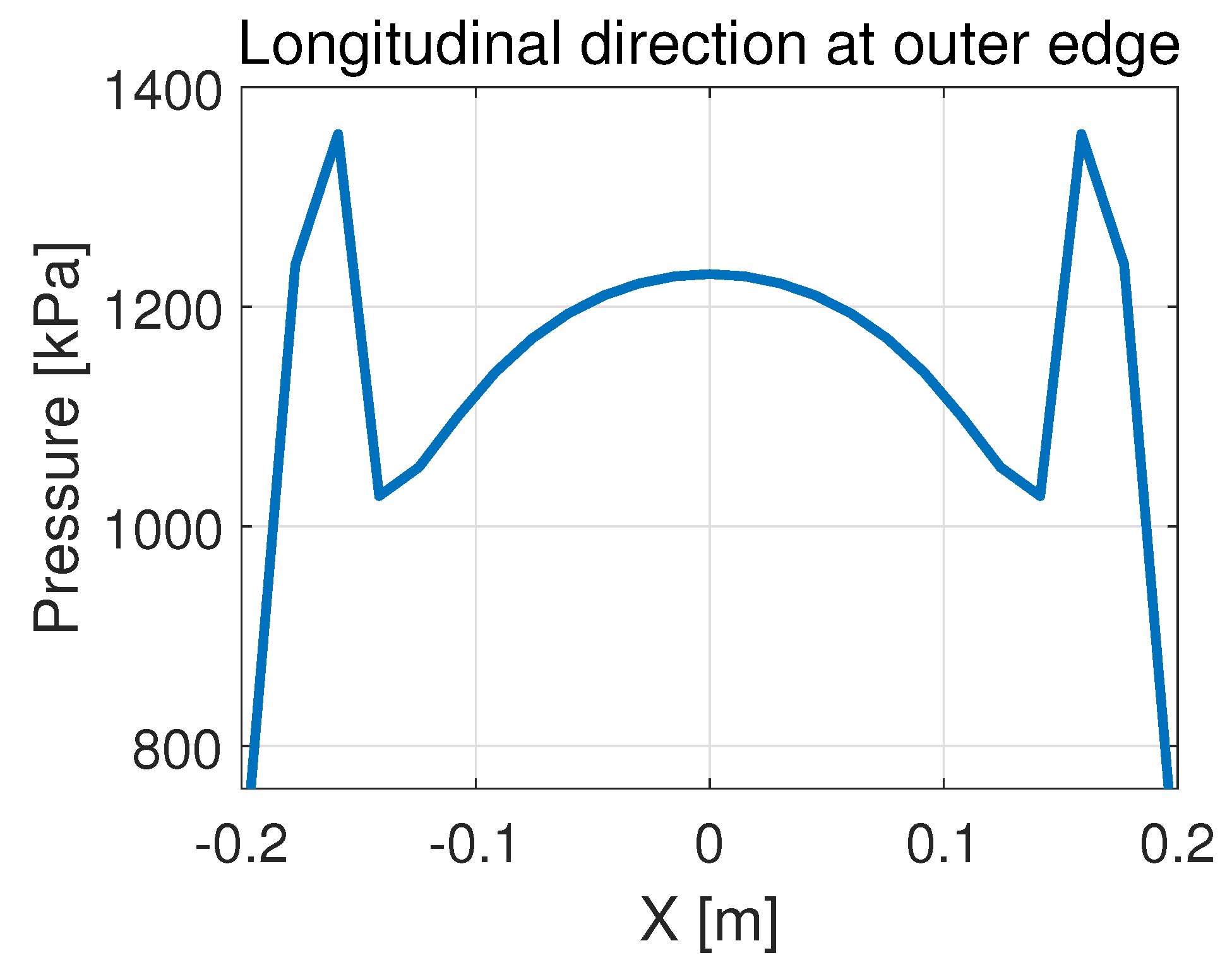
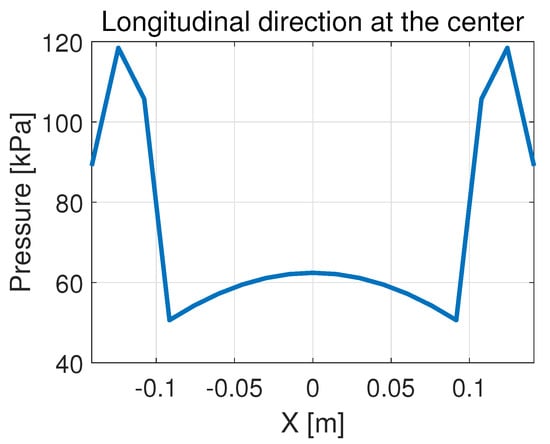
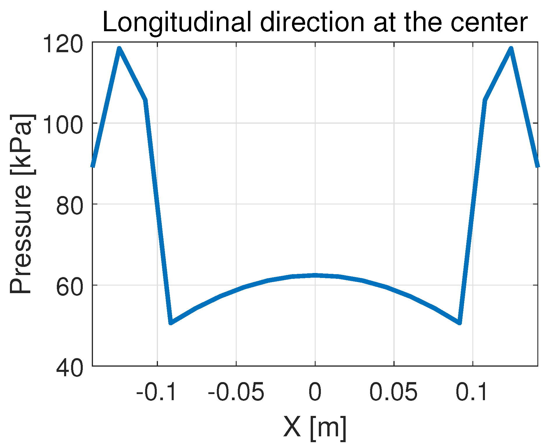
Overall, the isotropic shell tire model performs well in terms of predicting the spindle force. However, it is inferior in terms of the pressure distribution. When the modeled AT238/85 R16 tire undergoes a deformation of 100 mm, the pressure distribution in the longitudinal direction is as shown in Figure 17 and Figure 18:

Figure 17. Pressure distribution in the longitudinal direction near the side edge of the contact patch with the isotropic shell model.

Figure 18. Pressure distribution in the longitudinal direction near the center of the contact patch with the isotropic shell model.

The pressure distribution forms a saddle shape and reaches its maximum near the entrance and exit of the contact patch, which is unlikely to happen. This is the motivation of this study to include orthotropic properties for the shell.

4.3. Orthotropic Shell Tire Model

The same calibration process is performed with the data from the flat plate test and the 51 mm cleat test of the AT238/85 R16 tire. The following parameters are identified:

$$\begin{array}{c}\hfill \begin{array}{cc}\hfill E_{\alpha }& =1.111e7\hfill \\ \hfill {\nu }_{\alpha }& =0.1199\hfill \\ \hfill E_{\beta }& =8.159e5\hfill \\ \hfill {\nu }_{\beta }& =0.0088\hfill \\ \hfill P& =14842\hfill \\ \hfill {\alpha }_1& =6740\hfill \\ \hfill {\alpha }_2& =13585\hfill \\ \hfill {\alpha }_3& =4095\hfill \\ \hfill h& =0.015\hfill \end{array}\end{array}$$

(48)

The calibration results are shown in Figure 19 and Figure 20:

Figure 19. Calibration results with the orthotropic shell model.

Figure 20. Calibration results with the orthotropic shell model.

It is observed that the orthotropic shell model achieves improved performance during calibration compared with the isotropic model. The simulated results almost overlap with the experimental data for the flat-plate test. The RMSE is 331.90 N for the 51 mm cleat calibration and 274.26 N for the flat plate. The same set of parameters is then used to predict the spindle force when the tire is loaded by cleats of different sizes. For the cleats smaller than 51 mm, the results are shown in Figure 21 and Figure 22.

Figure 21. Spindle force prediction for a 25 mm cleat with the orthotropic shell model.

Figure 22. Spindle force prediction for a 38 mm cleat with the orthotropic shell model.

It cam be observed that the model slightly underestimates the spindle force for a 25 mm cleat as the deformation approaches 60 mm. On the other hand, the results are accurate for the 38 mm cleat. The RMSE for the 25 mm cleat and 38 mm cleat test are 227.79 N and 270.41 N, respectively. For cleats larger than 51 mm, the results are shown in Figure 23 and Figure 24.

Figure 23. Spindle force prediction for a 76 mm cleat with the orthotropic shell model.

Figure 24. Spindle force prediction for a 100 mm cleat with the orthotropic shell model.

The model makes accurate predictions for the 100 mm cleat with a minor underestimation as the deformation approaches 90 mm. The model overestimates the spindle force for the 76 mm cleat when deformation is around 60 to 70 mm, the curve falls back down as the deformation increases. The RMSE for the 76 mm cleat and 100 mm cleat test are 549.82 N and 403.56 N, respectively.

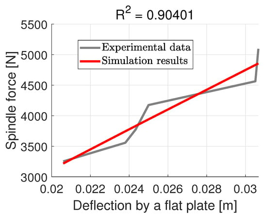
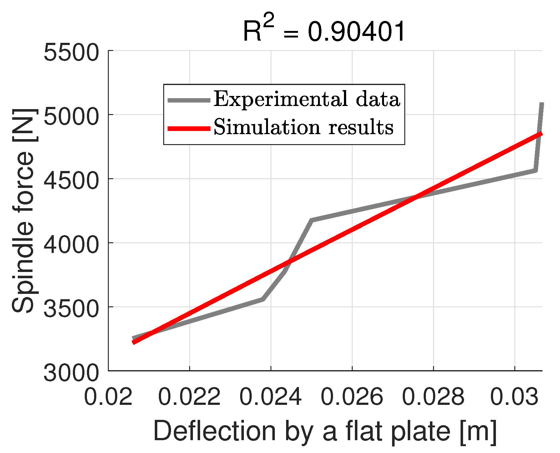
The model is then re-calibrated using the spindle force data of the SRTT to predict the normal pressure distribution. The calibration is shown in Figure 25.

Figure 25. Calibration results with the orthotropic shell model.

The spindle force is calculated based on the measurements from the pressure pad. The experimental pressure pad data differ from the normal force given by the wheel force transducer on the test rig. It can also be noticed from Figure 25 that the experimental values for the spindle force alternate on each side of the prediction of the orthotropic shell tire model. The following parameters are identified:

$$\begin{array}{c}\hfill \begin{array}{cc}\hfill E_{\alpha }& =1.3119e8\hfill \\ \hfill {\nu }_{\alpha }& =0.14527\hfill \\ \hfill E_{\beta }& =1.5933e8\hfill \\ \hfill {\nu }_{\beta }& =0.17643\hfill \\ \hfill P& =200000\hfill \\ \hfill {\alpha }_1& =16348\hfill \\ \hfill {\alpha }_2& =-29.2260\hfill \\ \hfill {\alpha }_3& =1.4820\hfill \\ \hfill h& =0.00298\hfill \end{array}\end{array}$$

(49)

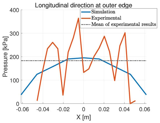
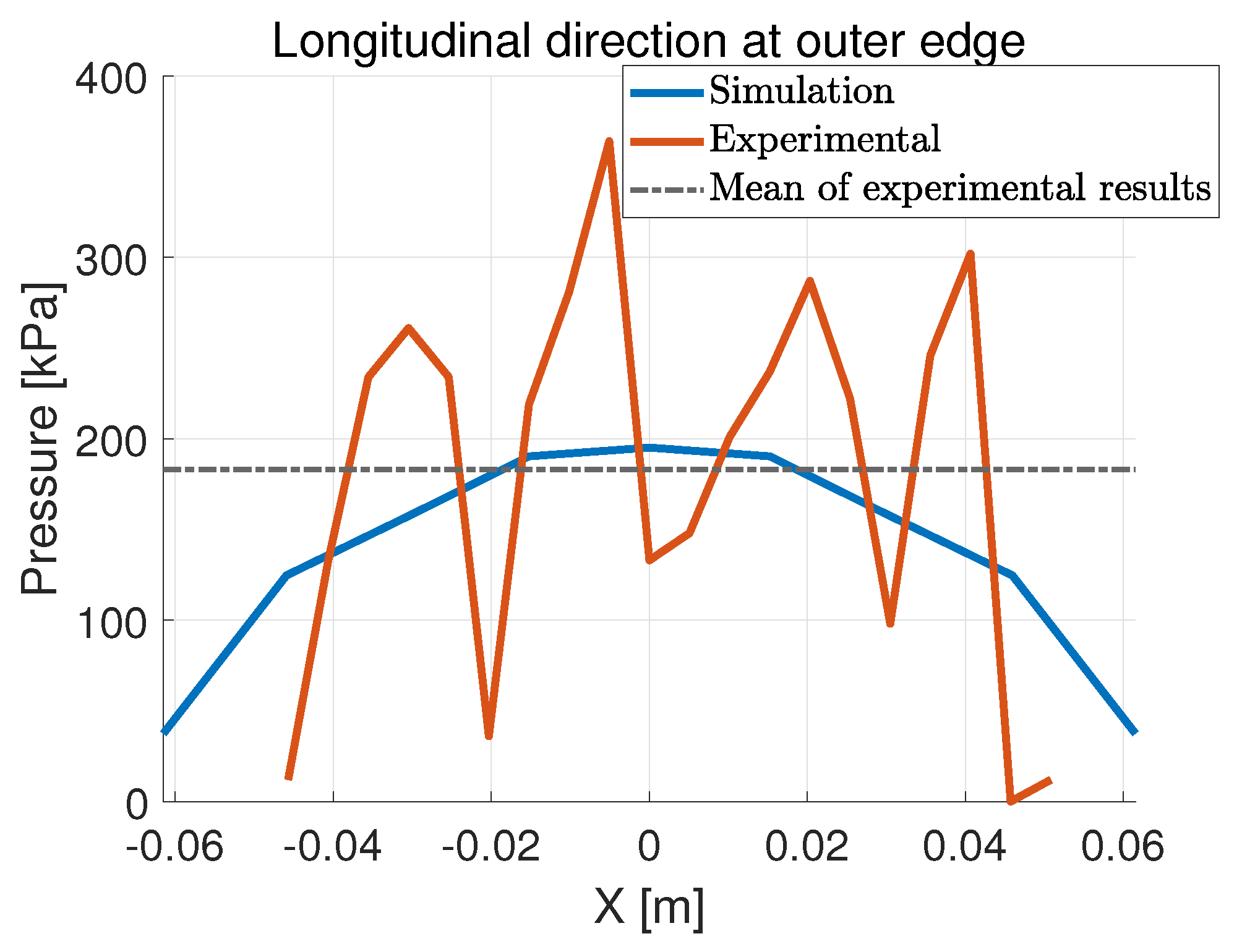
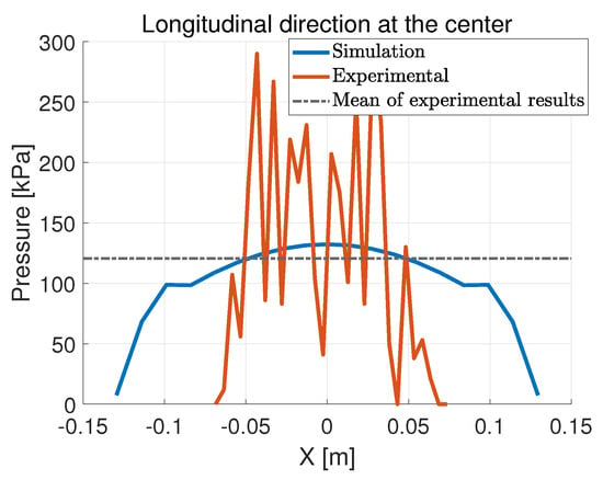
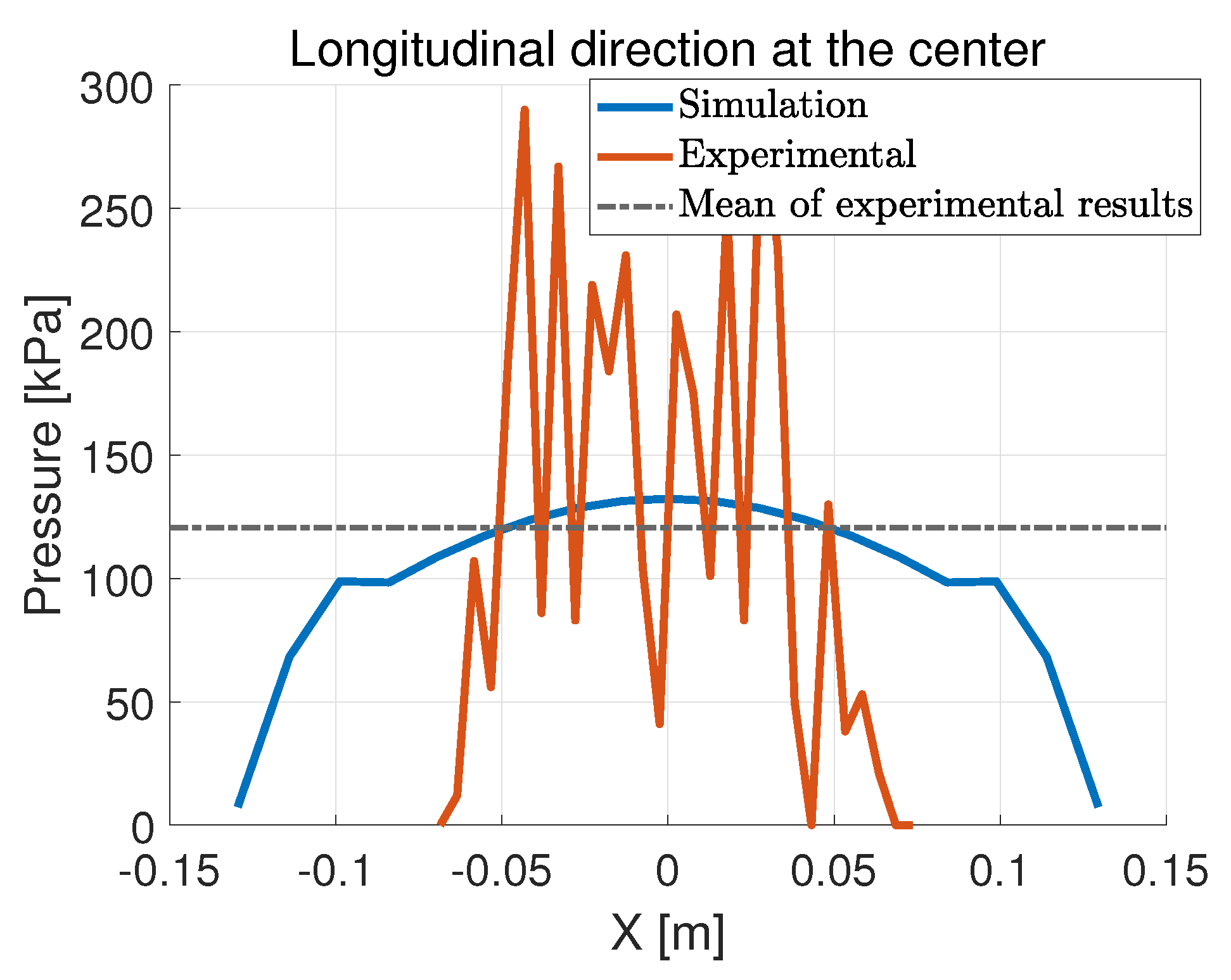
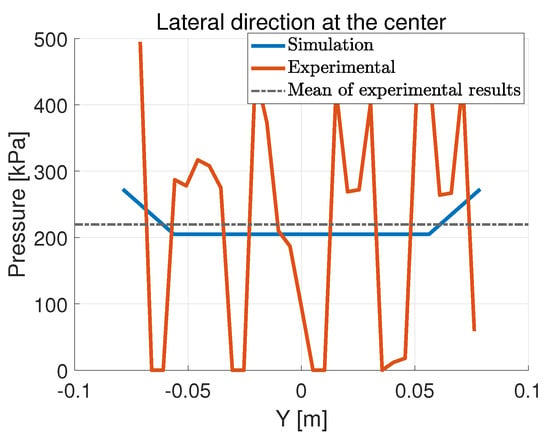
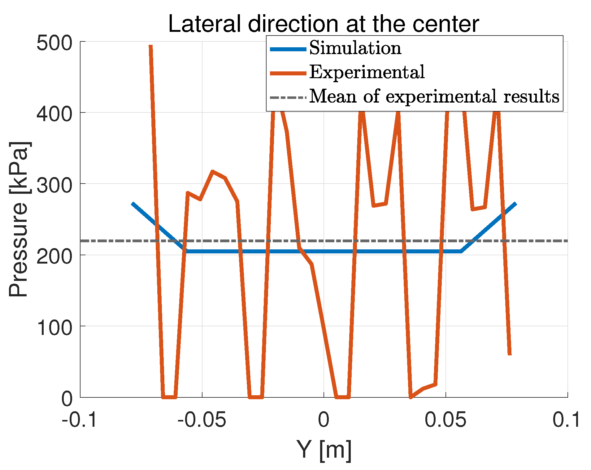
Comparisons are made between the simulation results and the experimental results for the SRTT, loaded by 28 mm with a flat plate (or rigid ground). The normal pressure is measured in two directions: lateral and longitudinal. In the longitudinal direction, the pressure is measured at the outer side and at the center of the contact patch, shown in Figure 26 and Figure 27.

Figure 26. Normal pressure distribution in the longitudinal direction with the orthotropic shell model.

Figure 27. Normal pressure distribution in the longitudinal direction with the orthotropic shell model.

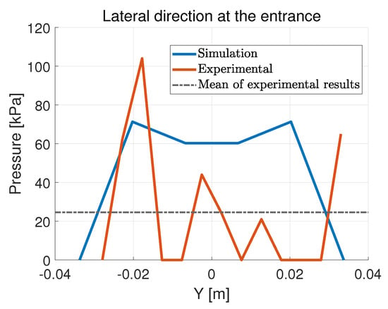
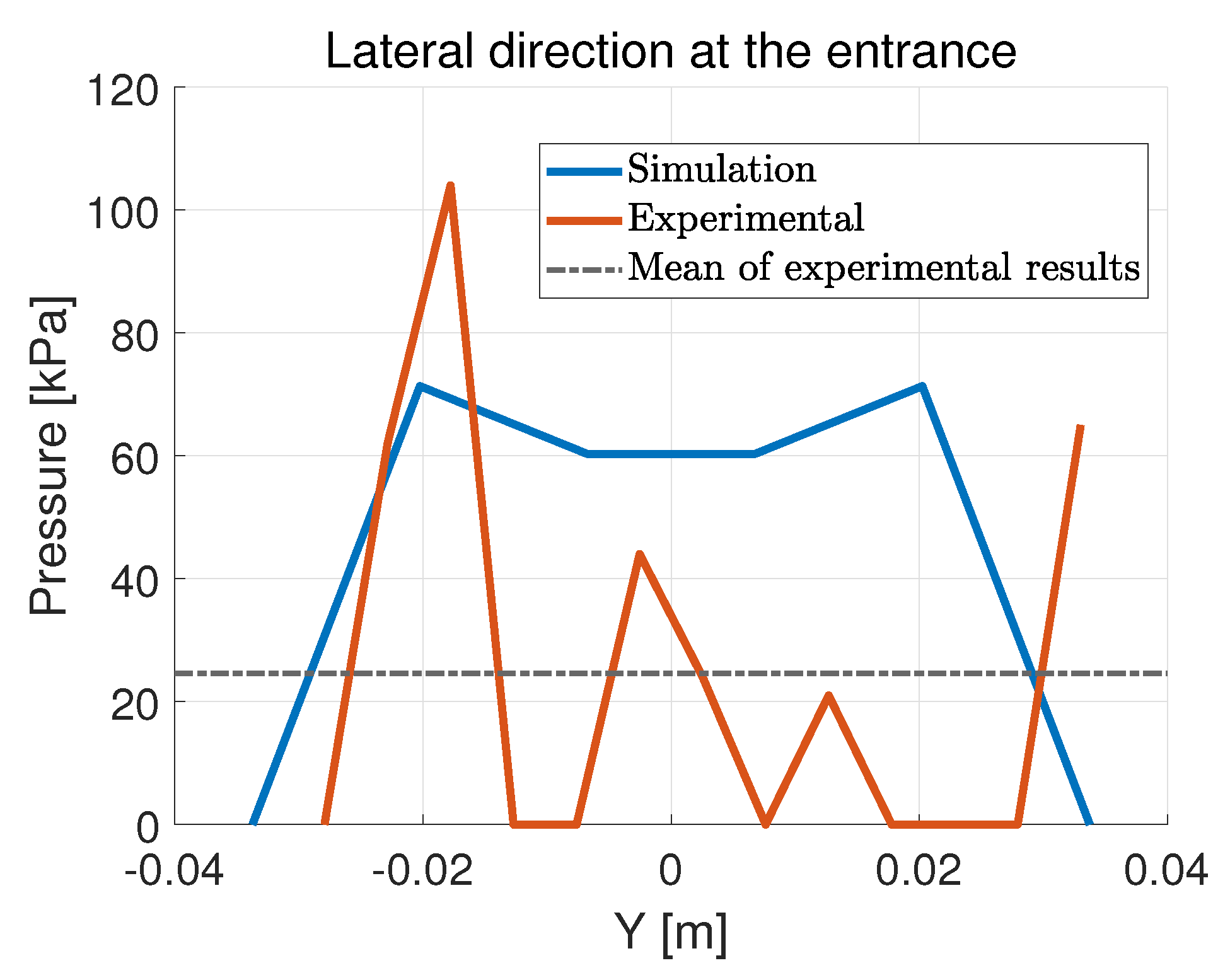
The zigzag shape of the experimental data is due to the grooves in the tread of the tire, which cannot be captured by the shell tire model. It is hard for the tread material inside of the groove to touch the pressure pad and generate readable data, causing local minima across the contact patch. The raised part of the tread, on the other hand, causes local maxima as it sustains all loads in its adjacency. The model tends to overestimate the size of the contact patch, especially at the edge. It can be observed that the simulation curve goes through the zigzag shape as a local mean of the local peaks and minima. The black dashed line denotes the mean of the experimental data, which is fairly close to the simulation curve. The RMSE between the simulated data and the mean value of the experimental data is 34.28 kPa at the outer edge and 8.37 kPa at the center. Similar characteristics can also be found in the lateral direction, as shown in Figure 28 and Figure 29.

Figure 28. Normal pressure distribution in the lateral direction with the orthotropic shell model.

Figure 29. Normal pressure distribution in the lateral direction with the orthotropic shell model.

The model tends to overestimate the pressure at the entrance of the contact patch while underestimating it at its center. It is demonstrated in Figure 29 that as the experimental curve zigzags through the contact patch, its global mean is very close to the simulation curve. The RMSE between the simulated data and the mean value of the experimental data is 34.14 kPa at the entrance and 17.58 kPa at the center.

5. Conclusions

The proposed tire model, which treats the tire as an elastic circular cylindrical shell on a nonlinear elastic foundation, is capable of capturing tire physics and predicting spindle force and normal pressure distribution. It offers rapid and low-cost calibration and estimates for tire performance, suitable for reliability studies and the initial design stage of a tire, and it can be expanded in the future to be employed in vehicle dynamics studies, owing to its connections among the model parameters and tire properties. The model takes significantly shorter computational time than finite element models. After calibration, it generally takes less than 3 s to calculate the spindle force, pressure distribution and deformation profile with MATLAB installed on an Intel i7 processor. Published FRM tire models generally take hours to complete a loading simulation, with [14] being a good example where the solving process is optimized to reduce computational time.

Future improvements can be carried out by calibrating with respect to more parameters and loading measurements. Most of the shell theories are developed from the stress–strain relationship on an infinitesimal element; they deal with small strain from the perspective of solid mechanics. These theories may introduce error when the curved surface of a shell is flattened, which is exactly the case for a tire model. The shell theory employed for a tire model could be modified to account for the flattening effects and greater strain (≈20–25%).

References

- Pacejka, H.B.; Bakker, E. The magic formula tyre model. Veh. Syst. Dyn. 1992, 21, 1–18. [Google Scholar] [CrossRef]
- Mashadi, B.; Mousavi, H.; Montazeri, M. Obtaining relations between the Magic Formula coefficients and tire physical properties. Int. J. Automot. Eng. 2015, 1, 911–922. [Google Scholar]
- Jansen, S.T.; Verhoeff, L.; Cremers, R.; Schmeitz, A.J.; Besselink, I.J. MF-Swift simulation study using benchmark data. Veh. Syst. Dyn. 2005, 43, 92–101. [Google Scholar] [CrossRef] [Scilit]
- Astrom, K.J.; De Wit, C.C. Revisiting the lugre model stick-slip motion and rate dependence. IEEE Control Syst. Mag. 2008, 28, 101–114. [Google Scholar]
- De Wit, C.C.; Olsson, H.; Astrom, K.J.; Lischinsky, P. A new model for control of systems with friction. IEEE Trans. Autom. Control 1995, 40, 419–425. [Google Scholar] [CrossRef] [Scilit]
- Piatkowski, T. Dahl and LuGre dynamic friction models—The analysis of selected properties. Mech. Mach. Theory 2014, 73, 91–100. [Google Scholar] [CrossRef] [Scilit]
- Lu, Y.; Zhang, J.; Yang, S.; Li, Z. Study on improvement of LuGre dynamical model and its application in vehicle handling dynamics. J. Mech. Sci. Technol. 2019, 33, 545–558. [Google Scholar] [CrossRef] [Scilit]
- Mashayekhi, A.; Behbahani, S.; Nahvi, A.; Keshmiri, M.; Shakeri, M. Analytical describing function of LuGre friction model. Int. J. Intell. Robot. Appl. 2022, 6, 437–448. [Google Scholar] [CrossRef] [Scilit]
- Wei, C.; Olatunbosun, O.A. Transient dynamic behaviour of finite element tire traversing obstacles with different heights. J. Terramech. 2014, 56, 1–16. [Google Scholar] [CrossRef] [Scilit]
- Shoop, S.A. Finite Element Modeling of Tire-Terrain Interaction; University of Michigan: Ann Arbor, MI, USA, 2001. [Google Scholar]
- Fervers, C. Improved FEM simulation model for tire–soil interaction. J. Terramechanics 2004, 41, 87–100. [Google Scholar] [CrossRef] [Scilit]
- Cueto, O.G.; Coronel, C.E.I.; Morfa, C.A.R.; Sosa, G.U.; Gómez, L.H.H.; Calderón, G.U.; Suárez, M.H. Three dimensional finite element model of soil compaction caused by agricultural tire traffic. Comput. Electron. Agric. 2013, 99, 146–152. [Google Scholar] [CrossRef] [Scilit]
- Chae, S. Nonlinear Finite Element Modeling and Analysis of a Truck Tire. 2006. Available online: https://etda.libraries.psu.edu/catalog/7047 (accessed on 31 August 2026).
- Horváth, E.; Tóth, C.; Kisgyörgy, L. Simulation of Static Tyre–Pavement Interaction Using Two FE Models of Different Complexity. Appl. Sci. 2022, 12, 2388. [Google Scholar] [CrossRef] [Scilit]
- Dugoff, H.; Fancher, P.S.; Segel, L. An analysis of tire traction properties and their influence on vehicle dynamic performance. SAE Trans. 1970, 1219–1243. [Google Scholar]
- Fiala, E. Seitenkraften am rollenden luftreifen. VdI 1954, 96, 973–979. [Google Scholar]
- Ding, N.; Taheri, S. A modified Dugoff tire model for combined-slip forces. Tire Sci. Technol. 2010, 38, 228–244. [Google Scholar] [CrossRef] [Scilit]
- Bhoraskar, A.; Sakthivel, P. A review and a comparison of Dugoff and modified Dugoff formula with Magic formula. In Proceedings of the 2017 International Conference on Nascent Technologies in Engineering (ICNTE); IEEE: New York, NY, USA, 2017; pp. 1–4. [Google Scholar]
- Villano, E.; Lenzo, B.; Sakhnevych, A. Cross-combined UKF for vehicle sideslip angle estimation with a modified Dugoff tire model: Design and experimental results. Meccanica 2021, 56, 2653–2668. [Google Scholar] [CrossRef] [Scilit]
- Gong, S. Study of in-Plane Dynamics of Tires. Ph.D. Thesis, Technische University, Delft, The Netherlands, 1993. [Google Scholar]
- Lee, H.; Taheri, S. A novel approach to tire parameter identification. Proc. Inst. Mech. Eng. Part D J. Automob. Eng. 2019, 233, 55–72. [Google Scholar] [CrossRef] [Scilit]
- Jeong, D.; Choi, S.B.; Lee, J.; Kim, M.; Lee, H. Tire dimensionless numbers for analysis of tire characteristics and intelligent tire signals. Mech. Syst. Signal Process. 2021, 161, 107927. [Google Scholar] [CrossRef] [Scilit]
- Ma, R.; Ferris, J.B.; Reid, A.A.; Gorsich, D.J. A planar quasi-static constraint mode tyre model. Veh. Syst. Dyn. 2015, 53, 1759–1771. [Google Scholar] [CrossRef] [Scilit]
- Liu, Z.; Gao, Q. Analytical investigation on tire dynamics by rigid–elastic coupled tire model with nonlinear sidewall stiffness. J. Braz. Soc. Mech. Sci. Eng. 2018, 40, 80. [Google Scholar] [CrossRef] [Scilit]
- Liu, Z.; Gao, Q. In-plane vibration response of time and frequency domain with rigid-elastic coupled tire model with continuous sidewall. Proc. Inst. Mech. Eng. Part K. J.-Multi-Body Dyn. 2018, 232, 429–445. [Google Scholar] [CrossRef] [Scilit]
- Tielking, J. Plane Vibration Characteristics of a Pneumatic Tire Model. In Mid-Year Meeting; SAE International: Warrendale, PA, USA, 1965. [Google Scholar]
- Koizumi, T.; Tsujiuchi, N.; Matsubara, M.; Nakamura, F.; Matsuyama, K. Vibration analysis of rolling tire based on thin cylindrical shell theory. In Proceedings of the ISMA, Leuven, Belgium, 20–22 September 2010; pp. 4003–4013. [Google Scholar]
- Roller, M.; Betsch, P.; Gallrein, A.; Linn, J. On the use of geometrically exact shells for dynamic tire simulation. In Multibody Dynamics; Computational Methods in Applied Sciences; Springer: Cham, Switzerland, 2014; pp. 205–236. [Google Scholar] [CrossRef] [Scilit]
- Roller, M.; Betsch, P.; Gallrein, A.; Linn, J. An enhanced tire model for dynamic simulation based on geometrically exact shells. Arch. Mech. Eng. 2016, 63, 277–295. [Google Scholar] [CrossRef] [Scilit]
- Bozdog, D.; Olson, W. Complex tire-ground interaction simulation: Recent developments of an advanced shell theory based tire model. In Proceedings of the Presentation at 2005 Tire Society Meeting; Citeseer: Princeton, NJ, USA, 2005. [Google Scholar]
- Bari, P.; Kanchwala, H. An analytical tire model using thin shell theory. Int. J. Mech. Sci. 2023, 248, 108227. [Google Scholar] [CrossRef] [Scilit]
- Sahu, G.N.; Kanchwala, H. Experimental modal analysis of a tire: An exploration of different operating and boundary conditions. J. Braz. Soc. Mech. Sci. Eng. 2024, 46, 667. [Google Scholar] [CrossRef] [Scilit]
- Bari, P.; Singh, A.P.; Kanchwala, H. A cylindrical shell model with distributed springs for a rotating tire. Int. J. Mech. Sci. 2024, 282, 109577. [Google Scholar] [CrossRef] [Scilit]
- Alujević, N.; Campillo-Davo, N.; Kindt, P.; Desmet, W.; Pluymers, B.; Vercammen, S. A simplified model of a rotating tire using cylindrical shells with free ends supported by an elastic foundation. In Proceedings of the ISMA 2014 International Conference on Noise and Vibration Engineering, Leuven, Belgium, 15–17 September 2014. [Google Scholar]
- Mikkola, A.M.; Shabana, A.A. A non-incremental finite element procedure for the analysis of large deformation of plates and shells in mechanical system applications. Multibody Syst. Dyn. 2003, 9, 283–309. [Google Scholar] [CrossRef] [Scilit]
- Xing, Y.; Liu, B.; Xu, T. Exact solutions for free vibration of circular cylindrical shells with classical boundary conditions. Int. J. Mech. Sci. 2013, 75, 178–188. [Google Scholar] [CrossRef] [Scilit]
- Shah, P.; Batra, R.C. Stretching and bending deformations due to normal and shear tractions of doubly curved shells using third-order shear and normal deformable theory. Mech. Adv. Mater. Struct. 2018, 25, 1276–1296. [Google Scholar] [CrossRef] [Scilit]
- Mohamadi, A.; Shahgholi, M.; Ghasemi, F.A. Nonlinear vibration of axially moving simply-supported circular cylindrical shell. Thin-Walled Struct. 2020, 156, 107026. [Google Scholar] [CrossRef] [Scilit]
- Guyan, R.J. Reduction of stiffness and mass matrices. AIAA J. 1965, 3, 380. [Google Scholar] [CrossRef] [Scilit] [PubMed]
- Leissa, A.W. Vibration of Shells; Scientific and Technical Information Office, National Aeronautics and Space Administration: Hampton, Virginia, 1973; Volume 288.
- Barber, J.R. Intermediate Mechanics of Materials; Springer: Berlin/Heidelberg, Germany, 2011; Volume 618. [Google Scholar]
- Xu, D. Improved Constraint Mode Tire Model with Analytical Derivations and Numerical Approximations. Ph.D. Thesis, Virginia Polytechnic Institute and State University, Blacksburg, Virginia, 2025. [Google Scholar]
- Clark, S.K. Mechanics of Pneumatic Tires; US Government Printing Office: Washington, DC, USA, 1981.
Disclaimer/Publisher’s Note: The statements, opinions and data contained in all publications are solely those of the individual author(s) and contributor(s) and not of MDPI and/or the editor(s). MDPI and/or the editor(s) disclaim responsibility for any injury to people or property resulting from any ideas, methods, instructions or products referred to in the content. |
© 2026 by the authors. Licensee MDPI, Basel, Switzerland. This article is an open access article distributed under the terms and conditions of the Creative Commons Attribution (CC BY) license.