


Abstract
Hydro-generator cooling arrays are sparsely instrumented, limiting estimation of heat-exchanger (HX) parameters from plant data for thermal modeling. This study develops and validates a 48-state quasi-linear parameter-varying (qLPV) gray-box model for twelve fin-and-tube air-to-water HXs in a hydro generator cooling system. Four equivalent three-HX groups use four serial cells each, and manufacturer-specified geometry and empirical correlations provide operating-dependent conductance values rather than fitted parameters. Of 19 coefficients, eleven are fixed, and eight effective group coefficients are estimated. Rated predictions reproduce manufacturer outlet temperatures within 0.6 °C, providing catalog-consistency verification. Coefficient calibration uses a 4.03 h window from a 48,241-sample (13.4 h) plant record. With the estimated coefficients frozen, combined filtered root-mean-square error (RMSE) values on the full record are 0.183 and 0.179 °C on the north and south sides of the cooler array. Multistart Nelder–Mead and direct four-dimensional simplicial homology global optimization (SHGO) yield numerically equivalent coefficient estimates. The resulting model is computationally economical and provides a physics-based plant-specific baseline for record replay, recalibration and prospective monitoring.
1. Introduction
Hydro power remains a cornerstone of the U.S. energy system and renewable energy generation. With a fleet numbering 2252 power plants and a generating capacity of 80.58 GW, hydro power contributed an average of 266 TWh annually between 2020 and 2022, representing 6.2% of total electricity generation and 28.7% of renewable electricity output in 2022, while also supplying 70% of utility-scale power storage capacity via pumped storage, thereby playing a vital role in grid reliability, renewable energy integration, and low-carbon power provision [1]. Hydro power is also important to grid flexibility in the context of variable loads and fluctuating power generation from other renewable sources. Flexible hydro-electric power generation, which has the ability to quickly respond to changes and provide load following, accounts for over 24 GW of firm capacity (i.e., guaranteed level of power that can be reliably produced) [2].
A generic hydro power plant consists of a storage reservoir, penstock, hydro-turbine, generator and powerhouse. The turbine-generator system, i.e., the electric power generation system, converts the kinetic energy of water flowing from the reservoir into electrical energy. The generator primarily consists of a stationary stator and a rotating rotor. The rotor is driven by a turbine runner through a common shaft assembly. These large-scale synchronous generators in hydroelectric power stations are among the most capital-intensive rotating machines in the energy sector, with individual unit costs ranging from tens to hundreds of millions of dollars and design lifetimes exceeding 40 years.
Hydro power generators, while achieving an overall system efficiency of more than 90%, are subjected to various losses during operation, such as I2R losses in stator and rotor windings, core losses (hysteresis and eddy current losses) in the stator and rotor, stray load losses, excitation system losses, and friction and windage losses that must be continuously addressed to prevent insulation degradation, winding deformation, and ultimately catastrophic failure [3,4,5]. The thermal life of insulation is approximately halved, i.e., the thermal aging rate is approximately doubled for every 10 °C increase in insulation temperature [6]. In addition, different materials heat up and cool down, and expand and contract at different rates, resulting in differential expansion. This introduces additional mechanical stresses and can crack insulation, delaminate insulation layers, and distort coils [7]. For example, in a 2009 survey examining failures that led to outages exceeding 10 days in hydro generators rated above 10 MVA, it was found that of 70 failures reported by 16 utilities across five different countries, 35 were attributed to insulation-related causes, 8 to thermal causes, 25 to mechanical causes, and 2 to bearing-related causes [8].
The reliability of hydro generators is of utmost significance to ensure power supply as required, with minimal or no disruptions. In addition to requiring repairs or maintenance and the ensuing downtime and financial losses, failure of generator components can also destabilize the electric grid. Effective cooling and thermal management of hydro generators can maintain operational efficiency, reliability and longevity of hydro generators and thus are of vital importance. A 1% loss in a 125 MW generator unit operating at rated power requires continuous removal of 1.25 MW of heat, and ambient cooling may not be sufficient. It should also be noted that thermal management refers not only to the limiting of peak temperatures, but also to maintaining a fairly uniform temperature profile in the generator. Large generators can have spots with insufficient ventilation, and localized heating may occur at those spots. Hence, dedicated cooling systems capable of effective cooling and thermal management are essential in hydro generators. The thermal management system typically comprises a closed-loop air ventilation circuit in which the rotor itself acts as a centrifugal fan, driving air over the active components and through banks of finned-tube heat exchangers (HXs) that transfer the waste heat to a river-water or chilled-water cooling circuit [9].
In their analysis of the cooling system of a 65 MW generator at the DEZ dam in Iran, Doost and Majlessi [10] noted that at rated power the losses amounted to 1.14 MW and when the inlet temperature of cooling water increased by 12 °C, the overall heat transfer efficiency of the cooling system dropped by 34%. The operators were then forced to drop load to prevent damage to the generators from overheating. Thus, heat exchangers in this system act as the primary thermal bottleneck. Any reduction in their heat transfer effectiveness, whether from air-side particulate fouling, biological growth on fin surfaces, water-side mineral scaling, or environmental shifts that induce wet-coil condensation, directly reduces the generator’s cooling capacity. Because the thermal losses increase with electrical load, and because the rotor speed (and hence the ventilation Airflow) is locked to the grid frequency, the generator operates with a relatively fixed thermal margin. A 10–15% reduction in heat exchanger effectiveness can be sufficient to push the winding hot-spot temperature beyond the Class F insulation limit of 155 °C, triggering protective relay action and forced derating or shutdown [4]. In the referenced measured data from the Rocky Reach unit, outlet-water flow is actively regulated in response to outlet air temperature deviations from its setpoint. In operation, alarm logic is implemented to prevent generator insulation temperatures from approaching their thermal limits.
Despite the criticality of these heat exchangers, installed cooler arrays are usually instrumented with only a small number of inlet and outlet temperatures and aggregate water-flow measurements. Vendor documentation is also designed primarily for equipment rating and commonly provides a rated duty, pressure drop, dimensions, and selected construction data rather than complete off-design conductance maps. The development and deployment of real-time, dynamic models of the heat exchanger system that are reliable, explainable and fast aids in condition-monitoring of such cooler arrays.
Broadly, modeling approaches of such heat exchanger systems can be of three types: Computational Fluid Dynamics (CFD) based methods, lumped parameter methods, and data-driven methods. Dang et al. [11] performed a CFD analysis of the convective heat transfer in the entire turbine heat generator system and validated their results using a small-scale experimental system. Such an analysis requires numerically solving fundamental mass, momentum and energy conservation equations over a fine mesh and can yield spatial profiles of temperatures. In contrast to CFD methods, lumped parameter approaches approximate an entire volume as a single node and consider uniform temperature across the node. Thus, these are much faster while sacrificing spatial detail. Pandey [12] shows a successful application of the lumped parameter approach in hydro generators using Bayesian parameter estimation. Jonsson et al. [13] present the use of an extended Kalman Filter coupled with a lumped state space model for dynamic modeling of heat exchangers. With recent advances in artificial intelligence approaches, Xayyasith et al. [14] and Huang et al. [15] used supervised machine learning and LSTM methods for modeling and fault detection in hydro generator cooling systems. In a parallel effort to this work, Li et al. [16] explored the use of distributed recurrent neural networks (dRNNs) in modeling the entire hydro generator cooling system. While CFD methods are computationally expensive and are not useful for real-time monitoring, data-driven methods suffer from a lack of data from a variety of operating conditions. It should be noted that traditional heat exchanger design and analysis methods such as the LMTD method or ε − NTU method have been used in the context of hydro generator cooling systems [9]. However, these methods are for steady-state analysis and may not be of good use in dynamically tracking the system behavior. Georgescu et al. [17] built a numerical model of the water side of the cooling system using EPANET and calibrated it using in situ measurements. Air-side heat transfer was not explicitly modeled in their work.
Dynamic state-space formulations based on lumped-parameter energy balances preserve the physical structure of the heat transfer process, enable fast/real-time monitoring while remaining suitable for standard observer and estimation techniques. Also, within the broader physics-informed modeling spectrum, recent work emphasizes that retaining governing structure can improve interpretability and data efficiency when observations are limited [18]. Accordingly, this study adopts a physically structured lumped state-space formulation. A key problem encountered in such an approach is the estimation of relevant heat transfer coefficients. Industries and vendors follow minimum reporting requirements, i.e., include only thermal and pressure rating values and operating conditions in the specification sheets as proposed in the AHRI 410 standard [19], while presenting a minimal amount of detail regarding the geometry of the heat exchangers. In this effort, we identify empirical correlations using the provided geometry information and incorporate the best applicable empirical correlations in the dynamic lumped parameter model.
The principal contributions of this paper are:
- A physics-based and computationally efficient quasi-linear parameter-varying (qLPV) model is developed for the complete twelve heat exchanger hydro generator cooling array. The model combines the geometry of the HXs with established air- and water-side empirical correlations to retain the operating-point-dependent heat transfer behavior of the real system.
- A reduced coefficient estimation formulation is introduced to complete the dynamic model using real plant measurements from limited instrumentation and unmeasured airflow. Four effective airflow and four outlet-blending coefficients are estimated, preserving the geometry and correlation-based thermal structure while enabling tractable periodic recalibration.
- The model is evaluated using 48,241 time series measurements from 13.4 h of real operation at an in-service 135 MW hydro-generator. The operating record was split into 4 windows, and the coefficients calibrated over one operating window were transferred unchanged to other windows as well as the full record. The combined filtered RMSE is 0.183 °C on the North side and 0.179 °C on the South side, with a cumulative water side energy difference of 0.330% between measured and predicted values.
- The study demonstrates that the reduced calibration is numerically reproducible, computationally practical, and robust to the recorded and tested variations in prescribed quantities. Independent optimization strategies yield equivalent predictions, and full-record simulation and filtering required less than 200 s on a regular computer, i.e., more than 200 times faster than real time.
The resulting model is tied directly to the measured outputs. For condition monitoring in future applications, using the estimated coefficients in this work can produce a reference/baseline response, while occasional offline re-estimation can be recorded separately as an effective-coefficient trend indicator.
This work focuses primarily on heat exchanger modeling in the cooling system, and water flow modeling and control are to be explored in future work. The remainder of this paper is organized as follows: Section 2 presents a brief description of the hydro generator cooling system considered in this paper, Section 3 presents the overall methodology and state-space formulation, and Section 4 presents parameter identification for the developed models. Section 5 presents the validation results against measured operational data and a discussion. Section 6 draws conclusions and identifies directions for future work.
2. System Description
This work primarily focuses on the circulating air-to-cooling-water heat exchanger system. The words cooler and heat exchanger are used interchangeably in this document. Figure 1 shows the components of a generic cooling system of a hydro generator and the fluid flow pathways. The solid black arrows represent the airflow cycle: hot air flows from the rotor and stator assembly into the cooler, where it loses heat energy to the cooling fluid, i.e., water, and cold air flows back into the assembly. The cooling unit at Rocky Reach Dam in Chelan County, WA, USA is the subject of this research effort.
Figure 1.
Generic cooling system in a hydro generator.
Figure 2 and Figure 3 show a top view of the assembly. The stator, the airflow ports, one heat exchanger and the water flow pipes are labeled. There are a total of 12 identical heat exchangers arranged uniformly around the generator assembly. These are divided into 4 groups for modeling purposes, as explained later in the document. There are 6 HXs on the north side and 6 HXs on the south side. As shown in the simplified version in Figure 3, the HXs on each side receive filtered cold water from the reservoir through a single supply pipe and discharge hot water into a single return pipe, making the HX array a parallel one on each side. Water flow is adjusted independently on each side based on the outlet air temperatures on that side.
Figure 2.
The cooling system considered in this work.
Figure 3.
Top view of the heat exchanger network and a simplified view of the heat exchanger assembly.
Instrumentation and Measurements: The generator cooling system is instrumented with 8 air temperature sensors, 4 water temperature sensors and 2 water flow rate sensors placed at select locations, providing 14 measurement channels sampled at 1 s intervals. Measurements are recorded separately for the north and south sides of the system as shown in Table 1. The groups shown in Figure 3 are named after the air temperature measurement locations.
Table 1.
Measurements in the considered hydro generator cooling system.
Heat Exchanger Design/Configuration: According to the manufacturer’s datasheet, the heat exchangers used in this unit are of the 1990s fin-and-tube design with wavy fins and have a thermal rating of 141 kW. The rated air and water volumetric flow rates are and . The construction materials are copper for tubes, aluminum for fins, brass for end plates and steel for other structural components. As shown in Table 2, following the reporting requirements from the AHRI 410 standard [19], the details presented in the spec sheet are very limited, i.e., only single-value thermal and pressure drop ratings are provided, and no information on flow-dependent heat transfer coefficients is included. These parameters are discussed in further detail in Section 3 and Section 4. Each HX consists of a 4-row 4-pass staggered tube bank with a wavy fin pattern. All geometry is evaluated once and remains fixed in every dynamic simulation presented later in this paper.
Table 2.
Specifications of the heat exchangers considered in this study.
The reconstructed geometry gives a minimum airflow area of 0.956266 m2 through the heat exchanger, i.e., between the fins and over the tubes, an air-side wetted area of 201.998 m2, a hydraulic diameter of 2.084 mm and an internal air volume of 0.371094 m3. The calculated metal heat capacity, including copper tubes, aluminum fins, brass end plates, and assigned structural steel, is 115.974 kJ/K per HX. These values are not fitted to the plant measurements.
Rotor-Driven Airflow: The cooling airflow is driven by the rotor acting as a centrifugal fan, with inter-pole channels functioning as impellers. There are vanes on the top and bottom of the rotor to guide the cold airflow back into the generator after reflection by the generator enclosure wall (see Figure 1). Since the generator rotor operates at a constant speed locked to the grid frequency, following the fan affinity law in Equation (1) [22] the air volumetric flow rate is approximately constant.
It should be noted that, in a real plant, rotor speed alone does not uniquely determine the air flow rate. The operating point is established in addition by the pressure loss curves of the recirculating airflow path, including rotor-stator passages, HX cores, i.e., gaps in HX fins and over the tubes, and any leakage passages around the HXs. Hartono [23] held a small-scale experimental rig at 2000 rpm and obtained inferred mass flows from 0.0939 to 0.1291 kg/s across two stators and three fan-blade configurations, confirming that geometry and circuit resistance can alter the airflow rates at fixed speed.
At 100% generator load, the measured air velocities (only point values) at the exits of HXs 1, 4, 7 and 10 were 3.2 m/s, 3.2 m/s, 2.9 m/s and 3.2 m/s respectively. These measurements establish a “similar” nominal outlet velocity at the four instrumented HXs. No time series airflow measurements are available and, as such, no temporal airflow variations are resolved. Given the fixed speed and unchanged system configuration over the considered short operation record (13.4 h, see Section 5.2), the present model therefore holds the nominal air velocities constant. Air density is evaluated using time series temperature measurements and thus mass flow rates vary with time. Any other variations, for example due to changes in rotor speed or changes in flow path such as blocked fin gaps in the heat exchangers or deformed fins or fouling of fin surfaces, etc., are out of the scope of this effort.
3. Dynamic Model of the Hydro Generator Cooling System
In this section, we present a 1D (1 dimensional) reduced-order dynamic model of the cooling system. Initially, we list the intended modeling scope, five assumptions considered, an instrumentation-based grouping of heat exchangers and present the equations of the dynamic model.
3.1. Modeling Assumptions and Intended Scope
The following assumptions are made in developing the dynamic model of the hydrogenator cooling system:
- Pipe dynamics are neglected. Heat transfer and capacitance, i.e., thermal storage, in the supply and return pipes are neglected. The pipe lengths are unknown, and it is the opinion of the system engineers that heat transfer in the pipes is negligible.
- Only sensible heat transfer is modeled on the air side. Dehumidification is neglected. Note that enclosure humidity, condensate generation, and HX surface temperatures were not measured. Our reasoning is as follows: At startup, the generator enclosure air is approximately at the ambient humidity level in the powerhouse. As this air recirculates through the HXs, moisture may initially condense on the HX surfaces. The recirculated air subsequently reaches an equilibrium condition. Since the generator enclosure is not completely airtight, the moisture infiltration rate and the resulting steady-state condensation rate at equilibrium are assumed to be negligible. The dehumidification transients during startup of the generator and any steady-state condensation are outside the scope of this study and will be studied in future research. Additionally, the humidity values in the enclosure are not measured. The manufacturer-specified 18.8% RH value at rated conditions is used as a constant for calculating air’s density, viscosity, conductivity and specific heat in the simulations. A sensitivity analysis showed that increasing RH to 80% produced less than 3% error in the results. The reported humidity sensitivity analysis assesses the influence of humidity on air properties, not the potential influence of condensation.
- Since branch-level water flow measurements are unavailable, the measured water flow rate is split equally between the 6 HXs on each side. This assumption is tested in the sensitivity analysis presented in Section 5.
- Airflow through each HX is assumed to be constant in line with the fan affinity law in Equation (1), since the generator rotor speed is locked to grid frequency. A reference volumetric airflow rate is estimated from fixed-point velocity measurements and computed flow cross-section areas, using temperature-dependent density. Non-uniform flow distributions within and across the HXs are not modeled. The considered reduced-order model cannot handle such behavior, and a comprehensive CFD analysis is required to resolve those effects.
- The twelve HXs array is divided into four groups with three HXs in each group. The HXs within each three-unit group have identical nominal geometry and operating conditions.
These assumptions preserve energy conservation, thermal storage, geometry, and operating dependence while keeping the model suitable for repeated time-domain simulations. The intended outcome is prediction of measured outlet temperatures. The model is not used to infer individual branch flows, internal temperatures, to assign a unique physical meaning to each fitted coefficient, or to provide unique fault isolation.
3.2. Aggregation of Heat Exchangers and Model Boundary
The six heat exchangers on each side are divided into two symmetric groups of three units. The spatial groups are denoted using
g ∈ = {1,4,7,10}
Each group contains three adjacent HXs and is represented by the inlet and outlet air temperatures at the correspondingly numbered HX. On the north side, Group 1 comprises HXs 1, 2, and 3 (quadrant 1 in Figure 3), whose collective thermal behavior is characterized by the air temperature measurements at HX1. Similarly, Group 4 comprises HXs 4, 5, and 6. The group labels correspond to the locations of available air temperature sensors; i.e., the name “Group 4” is used because it is characterized by measurements at HX 4. Groups 7 and 10 are defined similarly for the south side. This grouping is selected for three reasons:
- Consistency with available measurements: Air temperatures are measured only at HXs 1, 4, 7 and 10. Therefore, this grouping represents the finest spatial resolution that can be supported by this instrumentation. Any further decomposition would not be adequately supported by the available instrumentation.
- Use of system symmetry: All 12 HXs are nominally identical. Therefore, the four groups can share the same parameter functions/values and can be modeled using a single dynamic model. No additional unknowns are introduced relative to a single group model.
- Improved fault localization: Treating the two groups on each side as independent dynamical units enables the generation of group-specific residuals. These residuals could support future fault localization efforts by distinguishing fault effects localized to either group on each side. Grouping the entire array on a side into a single node/lump model would collapse these residual signals and thus reduce the diagnostic sensitivity for asymmetric faults. Although fault detection and diagnosis are out of the scope of this work, this grouping is chosen to support future diagnostic applications.
The two group models on one side have separate air paths but share the same measured side-level water inlet temperature and total water mass flow. Their water outlets are mixed to compute the predicted outlet temperature, which can be compared with the single water outlet temperature sensor measurement for that side. North and South sides are otherwise modeled independently. For a side s ∈ {N,S} with groups (g1, g2), the measured temperature inputs and outputs are:
where the subscripts (a,i), (a,o), (w,i) and (w,o) denote air inlet, air outlet, water inlet and water outlet, respectively.
3.3. Multi-Cell, Three-Node AMTD Model of the Cooling System
Each group of three HXs is modeled as one equivalent heat exchanger with lumped thermal nodes. Arithmetic Mean Temperature Difference (AMTD) is used as the main driver of heat transfer between the hot fluid and the heat exchanger wall, and between the heat exchanger wall and the cold fluid in the developed 1-D dynamic model [13]. Used by Vaitekunas [24], Mathisen and Morari [25] and Jonsson and Palsson [26], in the context of estimating heat transfer coefficients, the AMTD model was experimentally validated multiple times in the heat transfer research and engineering space. More recently, Gao et al. [27] utilized the AMTD-based lumped model for studying the transient responses of cross-flow heat exchangers in the context of varying inlet mass flow rates. The equivalent lumped HX has three times the extensive properties, i.e., heat transfer areas on the hot and cold sides and thermal capacitances on the air, metal and water sides of a single HX.
It should be noted that AMTD is a crude approximation of the logarithmic mean temperature difference (LMTD), which is a more accurate driver of heat transfer. AMTD model with a single cell, i.e., one thermal node for each element (air, metal and water) of the equivalent heat exchanger, can introduce a systematic positive bias in the predicted heat transfer rate relative to the exact LMTD. For the HXs considered, this bias is approximately +12–34% depending on the operating condition.
Multi-cell discretization along the airflow direction is a standard solution to address this bias. By dividing the equivalent heat exchanger into Nc identical cells, the AMTD approximation within each cell becomes increasingly accurate, while retaining the linear state-space structure. Yang et al. [28,29] reported that using two cells instead of one cell reduced errors from 28.6% to 1.6% in counter-current heat exchanger modeling. Using the rated inlet flow and temperature values from Table 1, with the model parameters estimated as shown in Section 4, the air outlet root mean squared error (RMSE) values for a single HX at rated conditions were: 4.5 °C for Nc = 1, 0.4 °C for Nc = 4 and 0.3 °C for N = 8.
Because the improvement beyond four cells is marginal, the equivalent lumped HX is divided into Nc = 4 cells along the airflow direction, consistent with the four-row, four-pass design of individual HXs. Each cell contains three thermal nodes: air, metal and water. Thus “multi-cell” represents spatial discretization, and “three-node” denotes the three thermal states within each cell.
The HXs considered in this design are physically cross-flow units with airflow perpendicular to staggered tubes carrying water. The water circuit consists of 4 passes, each containing 33 parallel tubes. Water flow reverses direction in the headers between successive passes. Figure 4 depicts the physical layout of the individual and equivalent lumped HX and the cells considered in the developed model. It should be noted that the multi-cell discretization for the 1-D dynamic model is performed along the airflow direction. The cells are in series along the airflow direction, and thus the throughflow air mass flow rate remains the same across all cells and equal to the per-group airflow rate. Similarly, the four water passes are represented as a series flow path through the cells, and the same water mass-flow rate passes through each cell.
Figure 4.
Physical layout of individual and equivalent lumped HXs and the multi-cell structure.
The cells are arranged as shown in Figure 5, with hot air entering the first cell (j = 1) and cold air exiting the last cell (j = Nc, here Nc = 4), whereas cold water enters at j = Nc and hot water exits at j = 1. This opposing-flow connection is a counter-current surrogate used to represent the four-pass cross-flow exchanger within a low-order 1D model, and is not an exact representation of the physical 3D flow field. Equations (4) and (5) present the air and water inlet temperature value assignments for each cell. With outlet fluid temperatures of one cell acting as inlet temperatures for the next cell, a group contains 3Nc = 12 states.
Figure 5.
Inter-cell connectivity and flow path.
The purpose of the cell discretization is simply to retain the temperature progression through the exchanger while preserving a low-order linear state structure. The governing equations can be written directly for a general cell j = 1,…,Nc and Multi-cell AMTD formulations of this type are well established for dynamic heat-exchanger modeling [28,29]. The three energy balance governing equations are:
- Air node:
- Metal node:
- Water node:
Note that group indices are omitted in Equations (6)–(8) for simplicity and as the model remains the same across all groups. Table 3 defines all variables and parameters used in the above dynamic model equations.
Table 3.
Hydro generator cooling system dynamic model variables and parameters.
Let nh = 3 denote the number of physical HXs represented by one group. The extensive properties, i.e., heat transfer coefficients (conductances) and capacitances used in the model (Equations (6)–(8)), are calculated using those of individual HXs as shown in Equation (9), where the subscripts g and HX denote properties of equivalent HX of a group and individual HX, respectively.
The per-HX conductance maps UAam,HX and UAmw,HX are calculated from empirical correlations, using the current flows and thermophysical properties. These empirical correlations are presented in Section 4 and represent pristine/ideal HX as denoted by super script “nom”. Here, Rt is the tube-wall resistance, Rf is the prescribed water-side fouling resistance, and Ai is the internal tube area. Group-specific air-side and water-side correction factors Ka,g and Kw,g enter the effective heat transfer coefficients as:
These correction factors can also represent performance degradation due to fouling or damaged fins, etc.
Note that each HX is made of multiple materials and thus the heat capacity of the lumped metal node is calculated as the sum of heat capacities of nm number of materials in the HX. A correction factor Km is used since the exact weights/volumes of individual metals in the HX are not given in the specification document. This correction factor is constant for all 12 HXs, since those are identical to each other. The baseline metal heat capacity of one HX is kJ/K.
The airflow rate for the group is calculated using an effective participating-airflow coefficient αg and nominal air velocity (discussed in Section 2) as shown in Equation (11), where represents the air density calculated as a function of time-varying inlet and outlet air temperatures and Ac,HX represents the minimum cross-section area for airflow between the fins and over the tubes in an individual HX. This is used in line with the empirical correlations discussed in Section 4. The participating airflow coefficient αg accounts for the correction between Ac,HX and the cross-section at the measurement location in an ideal case. Additional discussion on this parameter is provided in Section 4.
On each side, let ϕw,s, s ∈ {N,S} denote the fraction of the measured total water flow assigned to the lower-numbered group. Therefore, the water mass flow rate for group i:
where and are the cumulative water flow rates on the north and south sides, respectively. Within a group, water flow is divided equally among the three nominally identical HXs when the per-HX water-side correlations are evaluated. Using assumption 3 in Section 3.1, ϕw,s is set to 0.5 in the model. A sensitivity analysis is performed, and the results are discussed in Section 5.
3.4. State Space Assembly
With three states per cell and Nc cells per group, the state vector for a group g is and is stacked as:
The group input and output vectors are:
The continuous-time system is assembled by substituting the inter-cell connectivity in Equations (4) and (5) into the energy balances in Equations (6)–(8). The scheduling parameter vector Θ(t) contains the measured flows and temperatures, and the operating-dependent properties and conductance values evaluated at the current measurement interval, yielding a quasi—Linear Parameter-Varying (LPV) system. For compactness, group and time arguments are omitted in the coefficient definitions below from Equations (6)–(8):
These coefficients are the building blocks of the matrices Ag and Bg of the qLPV model. The 3Nc × 3Nc system matrix Ag is block-tridiagonal and takes the form:
Each diagonal block Dj is a 3 × 3 matrix containing the local cell dynamics (self-coupling) terms of cell j:
The sub-diagonal blocks Lj carry the air advection coupling where cell j − 1’s air outlet feeds cell j’s air inlet:
The super-diagonal blocks Uj carry the counter-current water coupling with cell j + 1’s water outlet feeding cell j’s water inlet:
The input matrix is sparse, with nonzero entries only in cell 1 (air inlet, column 1) and cell Nc (water inlet, column 2):
With Nc = 4, each group has 12 states. Stacking the four groups gives the 48-state qLPV model. The four air inlets remain separate while the two groups on each side share the corresponding water inlet. The matrices are reevaluated at each 1 s measurement interval, and the interval update uses exact zero-order-hold discretization during simulations.
3.5. Measurement Equations
Air Temperature Measurement Equation: A fraction of the total air mass flow bypasses the HX without any thermal interaction with the wetted surfaces. This bypassed air mixes with the thermally processed air, i.e., air that was in contact with the cooling surfaces and lost heat energy, which is at a reduced temperature before reaching the sensor. In addition to this unresolved outlet mixing, flow nonuniformity, other possible bypass paths, and sensor location affect air outlet temperature measurement.
For each group, the predicted air temperature at the outlet sensor is
where is the air outlet temperature from the last cell. The coefficient βg is an effective outlet-blending coefficient, and it is not interpreted as a direct measurement of a physical bypass fraction.
Water Temperature Measurement Equation: As mentioned in Section 2, only one outlet water temperature sensor is present on each side. Following modeling assumptions, for side s with groups (g1,g2), the single measured water-outlet temperature is modeled by the flow-weighted relation below. With the baseline equal split, ϕw,s = 0.5, it reduces to the arithmetic mean of the two predicted group outlets:
4. Parameter Estimation
4.1. Complete Model Coefficient Set and Classification
The 48-state qLPV model developed in Section 3 contains 19 potentially uncertain coefficients. These 19 coefficients are distinct from the propagated temperature states, the calculated air, metal, and water capacitances and the operating-dependent UAam,HX and UAmw,HX conductance values. The 19 coefficients comprise four air-side conductance multipliers Ka,g, four water-side conductance multipliers Kw,g, one common metal-capacitance multiplier Km, four participating-airflow coefficients αg, four outlet-blending coefficients βg, and two side-level water-flow allocation fractions ϕw,s. In this section, we present:
- The complete inventory of model parameters and coefficients;
- The calculation of operating-dependent air-side and water-side conductance values using the geometry of the HX and empirical coefficients;
- The setup of the optimization problem for computing a deliberately reduced set of coefficients.
Table 4 lists the number and role of each model quantity and its treatment in this work. The complete 19-coefficient inventory is:
ϑ = col({Ka,g}g∈,{Kw,g}g∈,Km,{αg}g∈,{βg}g∈,ϕw,N,ϕw,S) ∈ ℝ19,
= {1, 4, 7, 10}
= {1, 4, 7, 10}
Table 4.
Complete model parameter and coefficient set inventory and treatment.
Although all model coefficients could be treated as unknowns in a more extensively instrumented identification experiment, in this work we refrain from performing a formal 19-parameter identifiability analysis and estimation. Instead, we pursue a gray-box modeling approach with estimation of a reduced set of parameters from plant operating records using a physically prescribed dynamic structure. After the measured inlet temperatures and side-level water flows are treated as exogenous inputs, calibration uses only six outlet-temperature channels: four group air-outlet temperatures and two mixed side-level water-outlet temperatures. These outputs are correlated and do not include the branch airflow, branch water flow, local surface condition, or local outlet-mixing measurements required to separate all coefficient effects.
The four Ka,g coefficients, four Kw,g coefficients, Km, and the two ϕw,s coefficients are fixed, while the four αg and four βg coefficients are estimated. Km is tied mainly to installed metal mass and material heat capacity and is expected to remain approximately constant for unchanged hardware, although it remains an effective multiplier. The water-allocation fraction ϕw,s is governed by branch hydraulics and may be approximately constant while piping configuration and branch resistance remain stable. The eleven fixed coefficients are assigned nominal values based on geometry, material properties, symmetric piping assumptions, and empirical correlations applicable to the installed HX geometry and operating range. Their values should therefore be interpreted as physically informed modeling assumptions rather than independently identified plant-specific quantities. This treatment does not imply that all 19 coefficients could never be estimated from a different, deliberately instrumented experiment.
Our reasoning for this reduced coefficient estimation is as follows: We are not simply comparing the number of outputs and coefficients. The plant instrumentation is a decisive obstacle in identifying all 19 unknown parameters, since only six “processed” output channels with strongly correlated measurements are available in total. Multiple coefficients act on the same measurements through common pathways, while the branch quantities needed to separate their effects are not measured. For example, parameter αg affects the airflow rate, and consequently the air-side conductance UAam,g through Reynolds number, and the parameter Ka,g also scales the heat transfer rate on the air side, making their influences collinear under available operating excitation. Branch airflow is not measured, so αg is used as the single correction mechanism for unresolved participating airflow in each group. Outlet-air mixing and sensor placement are not resolved spatially, so βg is confined to the measurement equation. Estimating Ka,g together with αg and βg would allow these corrections to compensate through the same air-side heat-transfer and energy balance.
Similarly, confounding occurs between Kw,g and water allocation parameter ϕw,s. Additionally, the air-side and water-side parameters interact in the energy balance. Note that Km primarily affects metal node capacitance and thus storage and transient response. Because the data were collected during routine plant operation rather than a designed excitation experiment, it does not independently isolate or excite every conductance or capacitance, i.e., thermal storage, flow allocation, and air-side blending effect. Joint estimation of such collinear parameters from such a dataset can yield an ill-posed inverse problem in which some parameters can compensate for others.
The approach used is consistent with gray-box practice, in which prior physical knowledge specifies the model structure and a set of independently supported quantities, while data are used to estimate the remaining uncertain terms [30]. Example thermal studies use low-order physically structured models and add complexity only when supported by the available measurements [31,32]. Brastein et al. [33] showed that calibrating parameters of simplified lumped parameter thermal models from real measurement data can improve their accuracy and generalization capabilities and that reducing the degrees of freedom in thermal gray-box estimation can materially reduce dispersion among estimates obtained from different initial conditions. Reynders et al. [34] showed that the reliability of identified thermal parameters depends on the available input and observation signals. Broader hydropower precedents show how real plant operating records can support both hybrid dynamic modeling and offline parametric tuning, particularly [35,36] combined offline turbine calibration with online generator state and parameter updating, while identifying plant-specific recalibration and seasonality as issues requiring further evaluation. Complementarily, Kletschkowski [37] demonstrated that adaptive system identification can track condition-sensitive changes in model response. These references establish methodological precedent for operating-data calibration and model updating.
The reduced formulation remains useful because the prescribed structure retains energy conservation, thermal storage, serial temperature progression through the four cells, and operating dependence from the empirical correlations. The eight fitted coefficients provide plant-specific adjustment for unresolved airflow through the HXs and outlet-air blending while enabling prediction of the six instrumented outlet temperatures over observed load changes.
Within each calibration run, i.e., the analyzed interval for coefficient estimation, we treat the estimated values as time-invariant. These values can be re-estimated over new calibration windows. In a prospective long-term implementation, a normal-operation reference vector could be retained for temperature-baseline monitoring, while periodic re-estimation could be examined separately for apparent changes in the effective coefficients as operating or seasonal conditions change. Note that automatic replacement of the reference after every window could absorb a slowly developing anomaly, and a change in an effective coefficient is not a unique fault signature.
The UAam,HX and UAmw,HX values already vary sample by sample with the relevant operating variables and temperature-dependent properties. This dependence on operating conditions and fast variability should be distinguished from possible slow coefficient drift. In future research, Ka,g and Kw,g will be treated as slowly varying effective correction factors in the context of fouling, deposits, or surface-condition changes. Selected fixed quantities and assumptions are perturbed later using deterministic OFAT sensitivity calculations, and the results are presented in Section 5.7.
4.2. Calculation of Conductances and Capacitances Using Empirical Correlations and Geometry
The state-space model of Section 3 contains two thermal conductance values UAam and UAmw, three thermal capacitances Ca,HX, Cm,HX, and Cw,HX. The UAmw,HX and UAam,HX values are dependent on the water mass flow rate (measured) and the effective air mass flow rate, respectively and are computed using empirical correlations. Jönsson and Pálsson incorporated empirical heat-transfer relations into dynamic heat-exchanger models [26].
The water-side parameters (UAmw,HX, Cw,HX) depend only on known quantities from the specification sheet and known measurements: tube diameter, water flow rate, and water properties. In addition to the listed geometry parameters in Table 1, UAam,HX, Ca,HX, and Cm,HX, depend on two other unknown geometric quantities: the fin thickness δf and the wavy fin corrugation angle θ. The subscript HX is omitted in this section for simplifying the notation and compactness.
While δf and θ are not directly provided, three candidate fin thickness values were identified from the manufacturer’s website [20]: 0.0045 in (0.1143 mm), 0.0055 in (0.1397 mm), and 0.0075 in (0.1905 mm). Two specification-sheet quantities constrain these geometry unknowns: the total air-side cooling surface area Ao = 202 m2 and the air-side pressure drop ΔP = 93 Pa. Equation (24) calculates Ao which comprises the fin surface area without the tube hole punchouts and the exposed tube surface between adjacent fins [38,39]:
where Nf = ⌊Lx/Pf⌋ is the number of fins, Dc = Do + 2δf is the collar diameter, Hy is the face height, nr is the number of tube rows, Pl is the longitudinal pitch, Nt is the total number of tubes, Lx is the tube length, and Pf is the fin pitch. For a given δf, the calculated wavy fin angles are shown in Table 5.
Table 5.
Calculated fin corrugated angles using area constraint.
With θ* value fixed for each δf, Fanning friction factor f and Colburn j factor on the air side can be estimated using empirical correlations. These non-dimensional coefficients can then be used to estimate the air-side pressure drop ∆P and air-side conductance UAam using Equations (25) and (26) [40,41]:
where Ac is the minimum free-flow area, is the mass flux through the minimum free-flow area, and ρo are the HX inlet, mean and outlet air densities, and
where ηo is the overall external-surface efficiency obtained from the Schmidt fin efficiency [42], ka is the air conductivity, Dc is the collar diameter, ReDc is the air Reynolds number for flow over the collar diameter Dc and Pra is the air Prandtl number. Reshaeel et al. [43] provide a comprehensive list of such correlations. The friction factor correlations from [41,44,45] are considered, as they are developed for geometries that closely match the heat exchanger under study. Pressure drop and air-side conductance values are evaluated at each (δf, θ*) pair, producing a matrix of predicted pressure drop values presented in Table 6.
Table 6.
Pressure drop and air-side conductance values calculated using correlations from the literature.
The correlations that best approximate the specified pressure drop (93 Pa) and effective air-side conductance UAam,eff are chosen. UAam,eff is computed as follows: the overall thermal resistance of the heat exchanger decomposes into a series network:
where UAov is the overall thermal conductance of the HX and Rt is the metal tube wall resistance, kCu and kw are the copper and water thermal conductivities. The water-side conductance is computed using the Gnielinski correlation as shown in Equation (29), where fw = [0.79ln(Rew) − 1.64]−2 is the Petukhov friction factor [42]. The contact resistance that arises from the air gap between the expanded copper tube and the aluminum fin collar is not independently measurable in a field-deployed heat exchanger and is absorbed into UAam,eff. This approach is consistent with the catalog-data anchoring philosophy advocated by Rabehl et al. [46] for HVAC coil modeling.
Rt = ln(Do/Di)/(2π kCu Nt Lx)
The overall Conductance UAov is computed from specification data using the rated inlet and outlet temperatures (Ta,i, Ta,o, Tw,i, Tw,o), the rated heat duty Q, and the water volumetric flow rate using the P-NTU method with the analytical LMTD correction factor F for a cross-flow heat exchanger with nr = 4 tube rows and multiple passes [47] as shown in Equations (30)–(35).
The temperature effectiveness P and heat capacity ratio R are defined as:
The overall NTU on the water side, NTUw, is obtained by solving the Taborek P-NTU relation [47] for the specific flow arrangement (four-row, four-pass, cross-flow). The analytical framework provides the required closed-form expression. The analytical expression for P is:
A = 1/2κ(1 − κ/2 + κ2/4) + κ(1 − κ/2)(1 − 2Rκ(1 − κ/2))e2Rκ + (1 − κ/2)3e4Rκ
κ = 1 − exp(−NTUw/nr)
Calculating P and R from the specification data, Equations (31)–(33) are solved for NTUw, and the correction factor follows from:
The overall conductance is then computed:
where ΔTLMTD is the log-mean temperature difference for pure counter-flow, Th,i and Th,o are the hot fluid inlet and outlet temperatures, and Tc,i and Tc,o are the cold fluid inlet and outlet temperatures. The computed values were F = 0.987, which indicates that the rated crossflow/multi-pass arrangement has an LMTD close to that of an equivalent counter-flow exchanger. For the rated HX heat duty of 141 kW, the UAov value is 11.3 kW/K and the UAam,eff value is 14.15 kW/K.
The Wang et al. (2002) [41] correlation is selected as the primary model basis as it simultaneously achieves the closest pressure drop match and air-side conductance match to within 3% of the specification-anchored value for the (δf,θ*) pair 0.0075in and 17.78°. Wang et al. [41] also offer the widest experimental envelope with 61 samples spanning Dc = 7.66–16.85 mm, Pt = 21–38 mm, Pl = 12.7–33 mm, and Fp = 1.21–6.43 mm and an air-side Reynolds number range of 300–10,000, which fully contains the current geometry in Table 1 and provides the most reliable basis for off-design extrapolation. The Colburn j-factor is:
It can be observed that, for fixed geometry and approximately constant fluid properties, j has a power-law dependence of the form on air mass flow rate where c1 and c2 are purely geometric constants and are known completely. As seen in Equation (26), for a given j, in the dynamic model, UAam varies with temperature-dependent density, viscosity, conductivity, and Prandtl number.
The thermal capacitances Ca, Cm, and Cw are computed from the solved (δf,θ*) using simple geometry and known material properties. The metal capacitance Cm includes contributions from the copper tube walls, the aluminum fins, the brass end plates, and the steel frame. The final single-HX value is Cm,HX = 115.974 kJ/K. The fluid capacitances are Ca = Macp,a and Cw = Mwcp,w, where Ma and Mw are the lumped fluid masses within the heat exchanger.
Table 7 summarizes which of these vary with operating conditions and which remain fixed. The metal thermal capacitance Cm is constant with temperature, as the metal volume is fixed and the specific heats of copper and aluminum change negligibly over the 10–80 °C operating range. In contrast, the fluid capacitances Ca and Cw vary with the instantaneous fluid density and specific heat, which are temperature-dependent. The thermal conductances UAam and UAmw are nonlinear functions of the fluid properties ρ, cp, μ, and k, evaluated at the current air and water temperatures, respectively.
Table 7.
Operating condition dependence of the conductances and capacitances.
4.3. Reduced Optimization Problem
The αg and βg parameters for the north and south sides are estimated separately. For side s, let (g1,g2) = (1,4) for s = N and (g1,g2) = (7,10) for s = S. The two four-dimensional parameter vectors are
For each side, the three compared outputs are the two group air-outlet temperatures and the mixed side water-outlet temperature. With consistently preprocessed measured and predicted signals as described in Section 5.2, the residual for output r ∈ {a1,a2,w} is:
The equal-weight objective and the combined RMSE are:
where s is the sample set and Ns = |s|. The bounded estimation problem is
The bounds in Equation (40) encode engineering admissibility. The αg interval brackets plausible reconstruction error of the single air velocity measurement and keeps the collar-diameter Reynolds number inside the validated envelope of the conductance correlation, while βg bracket excludes the physically implausible regime in which the outlet sensor would read predominantly unprocessed inlet air. The two bounded problems use the same fixed model structure and coefficient treatment but are solved independently. The operating-record partition, numerical algorithms used, transfer tests, and results are discussed in Section 5.
5. Numerical Simulation and Results
This section evaluates the 48-state qLPV hydro generator cooling system model with manufacturer specification data and real plant operating records. The plant record and its division into multiple operating windows are described, followed by preliminary window-specific estimation of αg and βg coefficients and an across-window transfer analysis. The best-performing window is retained as the estimation window. Multistart Nelder–Mead and direct four-dimensional simplicial homological global optimization (SHGO) are subsequently used to corroborate the initial estimation results and to select the coefficients used in all remaining calculations. Full-record trajectories, error distributions, water-side thermal duty consistency and model performance metrics are then reported, followed by deterministic one-factor-at-a-time (OFAT) sensitivity results and a discussion of the model’s intended use and limitations.
5.1. Steady-State Validation at the Manufacturer-Rated Condition
The nominal single HX model with 4 cells was evaluated at the manufacturer-rated condition using the final geometry (888 fins and Dh = 2.08358 mm), the selected air-side and water-side correlations, the geometry-derived metal capacitance Cm = 115.974 kJ K−1 per physical HX, zero water-side fouling resistance, the nominal reduced-coefficient settings α = 1 and β = 0 and temperatures and flow rates listed in Table 8 (also Table 2).
Table 8.
Manufacturer-rated condition and nominal verification settings for one physical HX.
With model states initialized at temperatures of 30 °C the zero-order-hold discrete state-space model was propagated for 1000 s. The simulated air and water-outlet temperatures converge to 28.156 °C and 31.118 °C respectively, as shown in Figure 6. The corresponding steady-state errors are −0.5442 °C, and −0.1825 °C. Thus, the geometry- and correlation-based model reproduces the two catalog outlet temperatures to within 0.55 °C (1.9%). The remaining errors can be attributed to not considering heat transfer in the headers, u-bends and other mixing effects in the model, and the errors are comparable to those in the literature 1.6% [29].
Figure 6.
Response of the 4-cell AMTD model of a pristine single HX at manufacturer-rated conditions.
5.2. Plant Data and Analysis Windows
The operating record used in this analysis contains 48,241 consecutive one-second samples, corresponding to 13.4 h of plant operation. The complete-record measurements are summarized in Table 9.
Table 9.
Operating windows and measurement ranges.
Generator power varies from 89.14 to 133.12 MW. The four air-inlet channels span 49.31–56.80 °C at HX1, 48.27–55.55 °C at HX4, 49.73–57.84 °C at HX7, and 46.61–54.10 °C at HX10. The corresponding air-outlet ranges are much narrower: 24.37–25.20, 24.58–25.41, 23.95–24.78, and 24.58–25.41 °C, respectively. On the North side, water inlet and outlet temperatures span 9.40–10.03 and 21.67–22.71 °C, with total water flow from 39.13 to 54.41 m3h−1. The corresponding South-side temperatures are 10.24–10.65 and 23.95–24.58 °C, with total water flow ranging from 30.53 to 40.28 m3h−1.
The plant historian applies dead-band data compression, which produces plateaus of repeated values and discrete steps in the archived temperature readings. Values discarded before storage cannot be uniquely reconstructed from the available compressed record, and such a recovery of raw pre-compression measurements is outside the scope of this study. The discrete stair-step appearance of the measured values seen in Figure 7 should therefore be interpreted partly as a storage-resolution effect and not as thermal behavior that the model is expected to reproduce (it can be observed in the full record simulation results in Section 5.6 as well. See Figures 11 and 12).
Figure 7.
Recorded air-inlet temperatures and generator power with the identified operating windows.
Four contiguous operating windows are defined using the recorded generator power. A 61 s moving median is applied, and the largest centered 300 s absolute change score is taken within ±0.5 h of the pre-declared anchors at 1.0 h, 3.5 h, and 7.5 h. A minimum duration requirement of 0.5 h is enforced. The resulting sample edges are at 0 s, 2381 s (0.67 h), 13141 s (3.65 h), 27643 s (7.68 h), and 48241 s. As observed in Figure 7, Window 1 (W1) is a short high-load segment, W2 contains a sustained load reduction, W3 contains both increasing and decreasing load, and W4 contains the long final load drawdown. Table 9 lists the temperature, water flow and generator power ranges in each of the windows. Note that the listed values are the minimum and maximum unfiltered archived measurements within each window.
5.3. Numerical Implementation
The state space model developed in Section 3 is implemented independently for the two equivalent sides with two groups. For each generator side, the open-loop model receives the two measured group air-inlet temperatures, the common water-inlet temperature, and the measured total side water flow rate. The outputs are the two-group air-outlet temperatures and the common mixed water-outlet temperature. Generator power is used only to define the operating-window boundaries, and it is not an input to the thermal model. At ∆t = 1 s sampling interval, the discrete state update is:
where x[k] and u[k] are the state and thermal input vectors at time step k. At each one-second step, the thermodynamic properties of water and air, such as density, thermal conductivity, dynamic viscosity, specific heat and Prandtl number, are updated as functions of the respective mean temperatures in each cell and these properties are used to update conductance values and capacitances. The continuous-time state-space matrices A[k] and B[k] from Section 3 are then assembled, and their zero-order-hold discrete state-space equivalents Ad and Bd are obtained from the augmented matrix exponential [48]:
x[k + 1] = Ad[k]x[k] + Bd[k]u[k]
These matrices are used to propagate the open-loop state as shown in Equation (41). The Measured outlet temperatures are not used to correct the propagated state. Model inputs, i.e., inlet temperature measurements and flow rate measurements, are not filtered. For coefficient fitting and the reported filtered metrics, measured and simulated outputs are processed identically using a fixed second-order zero-phase Butterworth filter [49] with a cut-off frequency of 0.05 Hz, as used in prior work from our group for the same plant [50]. Up to 300 surrounding samples are used to reduce the filter-edge effects, and the first and last 200 samples of each scored interval are excluded.
Air properties are evaluated using a relative humidity (RH) value of 0.188 (18.8%) and at site pressure of 98.738 kPa to account for 218 m elevation. Humid-air density and humidity ratio follow the ASHRAE psychrometric formulation [51], mixing rules from Tsilingiris [52] and dry air properties from Lemmon et al. [53]. Temperature-dependent liquid-water properties are evaluated with the closed-form correlations of Popiel and Wojtkowiak [54]. The library CoolProp [55] was used offline only to validate implemented functions across the operating range. A TEMA-filtered river water fouling factor [56] was used as well (see Equation (10).
5.4. Effective α–β Coefficient Estimation and Multi-Window Temporal Transfer
The bounded optimization problem for reduced coefficient estimation in Section 4.3 was first solved separately for both the North and South sides on each of the 4 windows W1–W4 using the Nelder-Mead (NM) optimization algorithm [35,57]. Table 10 reports these initial estimates. Note that RMSE values are calculated using the 3 output measurements per side as shown in Equations (38) and (39) and not per group.
Table 10.
Initial window-specific estimates and own-window combined filtered RMSE.
The NM algorithm is gradient-free and evolves a simplex rather than an individual parameter vector. For the four-dimensional parameter vector used here, each iteration therefore uses five vertices, i.e., the objective is calculated at all five vertices, followed by ranking, reflection, expansion or contraction and shrink operations until stopping criteria are reached. One nominal initial vector sampled from within the coefficient bounds was supplied to the SciPy function [58], and the remaining four vertices were generated automatically.
Each search was limited to 200 optimizer iterations and used the absolute convergence tolerance of 10−3 for the maximum coordinate spread of the simplex and 10−4 °C2 for the maximum spread of the objective values. Successful termination required both conditions to be satisfied; otherwise, the search ended at the iteration limit. All eight W1–W4 side-window searches satisfied the stopping conditions before the limit and required 110–135 objective evaluations. Table 10 reports their terminal estimates.
Each window-specific and estimates were frozen and used across all other windows, including the full 13.4 h record, without re-estimation, and RMSE values were computed in each target window. Figure 8 is the resulting source-by-target temperature-error matrix. Diagonal entries are within-window RMSE estimates, and off-diagonal entries measure transfer to nonoverlapping windows. Accordingly, the term “multi-window validation” is used here only in this within-record sense and does not represent validation with an independent experiment, date, season, unit, or sensor configuration. Note that the full-record column contains the source window and is therefore supporting descriptive evidence, not out-of-sample evidence.
Figure 8.
Cross-window filtered RMSE. Rows denote the coefficient estimation source window, and columns denote the evaluation target window.
W1 gives the smallest own-window error but transfers poorly across other windows, consistent with its short duration and narrow load range. W2 transfers more consistently, but it contains a load reduction principally. W3 contains a bidirectional load excursion and gives the lowest error among the windows for which a later target exists (W4), i.e., the RMSE values were 0.184818 °C on the North side and 0.171510 °C on the South side when transferred temporally forward to W4. Coefficients estimated from W3 also explain the full record data better, and W3 is therefore retained as the estimation window considering operating content and forward temporal transfer within the record. Table 11 lists the cross-window transfer results. Note that “Forward” pools all later windows, and W4 has no later target.
Table 11.
Window-transfer summary for the initial single-start estimates. Highlighted cells represent minimum values over the full record.
5.5. Corroboration of Estimated Coefficients and Final Coefficient Selection
After W3 was retained as the source window for estimation, the bounded four-dimensional optimization problem for each generator side was repeated from 16 nominal starting points using the NM algorithm to examine the sensitivity to initialization. The starts comprised the initial W3 estimate, the center of the admissible parameter box from the bounds, and 14 Latin-hypercube sampled points. Every calculation used the same W3 data, model, coefficient bounds, preprocessing, and stopping settings. Figure 9 and Table 12 present the multi-start Nelder-Mead optimization results on W3. Fourteen North-side and 15 South-side runs returned completed optimization within the defined 200 iterations. This indicates meeting the configured termination criterion, and in Table 12, “same numerical solution” requires both an objective within 1% of the best value and a maximum absolute coefficient difference no greater than 0.01 from the best vector. Figure 9 documents the progression of the configured searches by plotting the trajectories of the best estimate of the objective in each iteration.
Figure 9.
Best objective histories in each iteration for the 16 multi-start Nelder–Mead searches using W3 data on both sides.
Table 12.
Multi-start Nelder–Mead summary on W3.
The lowest-objective runs resulted in coefficient vectors (α1, β1, α4, β4) = (0.861958, 0.232246, 0.981402, 0.217166) and (α7, β7, α10, β10) = (0.846637, 0.191922, 0.839205, 0.218375), respectively. The associated W3 objectives are 0.0548603 and 0.0553136 °C2, corresponding to combined RMSE values of 0.135229 and 0.135786 °C.
Seven North-side and eight South-side starts terminate within 1% of the best objective. Within that deterministic near-best set, the coefficient ranges are 0.861462–0.891367, 0.224731–0.232358, 0.949416–0.981963, and 0.217031–0.225463 on the North side, and 0.804016–0.866339, 0.186093–0.204470, 0.818965–0.886379, and 0.203184–0.224894 on the South side. These spans summarize the near-optimal terminal-solution dispersion obtained under the stated 1% objective threshold and sixteen separate initializations relative to the selected values.
A direct four-dimensional simplicial homology global optimization (SHGO) calculation [59,60] was then performed over the same bounds and W3 objective using 128 simplicial sampling points, two global iterations, and bounded Sequential Least Squares Programming (SLSQP) refinement. Figure 10 and Table 13 present the results comparing the different optimization methods. The maximum absolute difference between the selected multi-start NM and SHGO coefficients is 1.07 × 10⁻⁴ for the North side and 5.39 × 10⁻⁵ for the South side, and the corresponding differences between the objectives are 5.32 × 10⁻⁸ and 1.15 × 10⁻⁷ °C2. When propagated over the full record, the maximum difference between the two filtered trajectories is 2.75 × 10⁻⁴ °C for the North side and 3.13 × 10⁻⁴ °C for the South side. Thus, the two algorithms produce numerically equivalent predictions under the specified W3 window.
Figure 10.
Comparison of optimization results when using different methods on W3.
Table 13.
Comparison of optimization results when using different methods on W3 and final coefficient selection (highlighted).
The selected coefficients correspond to the lowest objectives among the 16 configured multi-start NM runs, and SHGO is retained only as an algorithmically distinct corroboration step. SHGO’s marginally smaller reported objectives are below meaningful reporting precision and yield indistinguishable trajectories. Note that neither W4, the temporally forward window, nor the full record is used in the estimation. The close numerical agreement provides strong evidence that the reported bounded estimation on W3 is robust to the tested initializations and optimization methods. Multi-start NM and direct SHGO return essentially the same strictly interior best solution on both the north and south sides. At the resolution of these searches, the results are consistent with one numerically resolved optimum within a shallow near-optimal region. This evidence supports a reproducible, predictive plant-specific calibration conditional on the adopted model and operating record.
Appreciable differences in the South-side coefficients from the initial single-start estimate can be observed, despite an RMSE reduction of only about 0.00236 °C on W3 data. This observation indicates that appreciable coefficient changes can occur within a nearly equivalent prediction region and cautions against assigning the coefficients unique physical meanings. The α and β values are therefore interpreted as effective reduced-model coefficients conditional on the adopted structure, eleven fixed coefficients, W3 data, preprocessing, and bounds and not as unique measurements of separable airflow, bypass, fouling, or sensor mechanisms.
No probabilistic parameter uncertainty is reported. Dispersion among solutions from different optimization methods is algorithmic in nature and is not a confidence or credible interval. Producing uncertainty bounds would require verified sensor characteristics, an explicit stochastic measurement-error and residual-correlation model, and preferably independent or repeated operating records, which are not available for this study. The presented coefficient estimation is consistent with the purpose and scope of the current effort, i.e., to establish and validate a reduced operational baseline for short-term prediction of outlet temperatures.
5.6. Full-Record Results with the Selected W3 Coefficients
The selected multi-start NM W3 coefficient vectors were frozen and propagated over all 48,241 one-second samples without re-estimation or state correction. On the subsequent W4 interval, the combined filtered RMSE is 0.184383 °C for the North side and 0.166957 °C for the South side. Over the full record, the corresponding values are 0.183305 and 0.178582 °C. Figure 11 and Figure 12 depict the full record simulation results using the selected coefficients.
Figure 11.
North-side full-record predictions using the selected multi-start NM coefficients estimated from W3 data. Vertical lines mark the W1–W4 boundaries.
Figure 12.
South-side full-record predictions using the selected multi-start NM coefficients estimated from W3 data.
To avoid relying on RMSE alone, Table 14 reports the mean absolute error (MAE), mean signed error, error standard deviation, and 95th-percentile absolute error. For the signed metrics and histograms in this subsection, error is defined as measured minus simulated temperature. The same 200 s guards are removed at the two outer record boundaries, leaving 47,841 samples per output. Figure 13 shows the corresponding empirical error distributions.
Table 14.
Filtered full-record performance with the selected multi-start W3 coefficients (N = 47,841 per output; error = measurement − simulation). Temperature-error metrics are in °C.
Figure 13.
Filtered full-record error histograms using the selected multi-start NM coefficients from W3 data.
Across the six channels, RMSE ranges from 0.137 to 0.219 °C, MAE from 0.111 to 0.181 °C, and the 95th-percentile absolute error from 0.271 to 0.418 °C. The largest absolute value of mean error is 0.061 °C. The trajectories reproduce several broad operating excursions and retain channel-dependent offsets and local deviations. The open-loop thermal model remains input-driven, causal, and directly reusable when operating conditions change. The thermal-duty comparison below provides an additional evaluation over a wider operating range.
At each time step, the archive-derived water-side thermal duty was calculated as the product of measured mass flow, water specific heat, and the measured outlet-minus-inlet temperature difference and was used for a water-side thermal-duty consistency check. The model-derived duty was calculated in the same manner but with simulated water-outlet temperatures. The same prescribed zero-phase filter was applied to both derived duty series for pointwise comparison, whereas cumulative energy was integrated from the unfiltered duties. Figure 14 depicts the north, south and combined water side measured and simulated thermal duties over the full record. It can be seen that the model-predicted values closely follow the values computed from flow and temperature measurements.
Figure 14.
Filtered archive-derived and model-predicted water-side thermal duty over the full operating record. Vertical lines mark the W1–W4 boundaries.
Using the selected multistart W3 coefficients, the full-record water-side duty RMSE is 11.6019 kW for the North side, 5.5121 kW for the South side, and 16.1625 kW for the total system. Because error is archive-derived minus model-derived duty, the negative mean errors denote average model overprediction of 2.5146, 1.5756, and 4.0903 kW, respectively. For the total system, the unfiltered cumulative energies over the guarded record are 16.4857 and 16.5401 MWh (thermal), a model-minus-archive difference of +0.33%.
5.7. Deterministic OFAT Sensitivity Analysis
The selected multi-start NM coefficients from W3 were held fixed while selected prescribed factors were varied one at a time over the complete record. The scenarios change the air-side conductance multiplier Ka, the water-side conductance multiplier Kw, the assumed allocation of total side water flow between the two groups ϕw,s, and the constant relative humidity. The OFAT sensitivity analysis results are presented in Table 15.
Table 15.
Full-record OFAT results while perturbing the 11 fixed coefficients. Combined filtered RMSE, °C and ΔRMSE relative to the baseline on the same side are listed.
Over the tested perturbations, the largest increases in combined RMSE arise from the air-side multiplier and the assumed water-flow allocation. A ±10% air-side multiplier change produces mean absolute shifts of approximately 0.41–0.56 °C in the air-outlet predictions. The water-side multiplier perturbations produce smaller but material air-output shifts of approximately 0.25–0.36 °C. Redistributing 10% of the side flow produces air-outlet shifts of approximately 0.44–0.69 °C, whereas the mixed water-outlet shift remains below about 0.055 °C because opposing group-level effects partially cancel in the common outlet mixture. The result shows that the unmeasured branch allocation is influential, but it does not supply enough independent information to add that allocation to the reduced estimation vector.
Relative humidity has a much smaller effect over the tested sensible heat transfer record. Changing the prescribed value from the 18.8% baseline to 50% increases combined RMSE by approximately 0.005 °C on either side, and the 80% case increases it by approximately 0.015 °C. The small negative ΔRMSE at 10% RH denotes only a marginal deterministic residual reduction.
5.8. Discussion
The model is intended to provide a plant-specific, open-loop thermal baseline at the spatial resolution supported by the installed instrumentation. From the measured inlet temperatures and side-level water flow, it predicts two group air-outlet temperatures and one common mixed water-outlet temperature per generator side. Appropriate uses include operating-record replay, examination of normal thermal response over observed load changes, periodic reduced-coefficient recalibration, and prospective residual-based monitoring using group-level residuals, while retaining computational speed for repeated and real-time simulations.
Table 16 positions the current work’s contribution against representative studies selected for similarity in application, HX construction, or modeling objective. The considered studies span hydro-generator cooler assessment, fin-and-tube correlation development, data-center crossflow air-to-water heat exchanger modeling, and dynamic reduced-order methods. Each entry in the “results accuracy” column retains the metric and validation basis used by its source. A direct one-on-one comparison with the current study is not possible (except with [16]) due to the differences in system design, scale and components. The listed values compare scope and evidence and are not evidence of numerical ranking across different machines, datasets, and prediction targets.
Table 16.
Representative hydro-generator, fin-and-tube, and reduced-order heat-exchanger studies. Reported errors retain each source’s definition and validation basis and are not directly rankable across rows. Highlighted rows indicate the current study and another one [16] performed on this generator cooling system at Rocky Reach (unit C08).
The selected literature provides complementary levels of description. Hydro-generator field studies [9,10] establish the operational importance of cooler condition and water temperature but are primarily steady analyses. Generator machine-level thermal networks prioritize online speed [61] and laboratory or generic HX studies develop transient reductions and flow-dependent correlations. The present work combines these strands at the operating cooler-array level. The principal methodological advantage in this study is the combination of a physically prescribed dynamic structure with empirical correlations that generate geometry- and operating-dependent air- and water-side conductance values and limited data-based adjustment of only 8 measurement-facing effective coefficients, which are calibrated from plant data. These effective quantities can absorb installation- and aggregation-dependent effects that the available measurements do not resolve separately. Restricting the decision vector in this way makes bounded batch recalibration practical and limits compensating changes among coefficients. Related plant-data hydropower and structured thermal-model studies provide broader context [35,63].
The results provide consistent evidence at temperature, thermal-power, and cumulative-energy scales. The rated calculation reproduces both manufacturer outlet temperatures within 0.6 °C. With the W3 coefficients frozen, subsequent W4 combined RMSE is 0.184 °C on the North side and 0.167 °C on the South side; the corresponding descriptive full-record values are 0.183 and 0.179 °C. Across the six temperature channels, full-record RMSE ranges from 0.137 to 0.219 °C, MAE from 0.111 to 0.181 °C, and P95 absolute error from 0.271 to 0.418 °C. Total-system water-side duty RMSE is 16.16 kW, and model-derived cumulative thermal energy differs from the archive-derived value by 0.330%. Forward propagation is computationally economical in the demonstrated implementation. Sequential simulation and output filtering of 48 states, in total over 48,241 samples representing 13.4 h, required less than 200 s in the recorded run on a regular laptop. The reduced calibration is also reproducible and computationally economical. W3 spans 4.03 h and contains a bidirectional load excursion, and its stronger forward transfer identifies it as more informative than the short and concentrated W1 or W2 with only load reduction. Multi-start Nelder–Mead and direct four-dimensional SHGO recover numerically equivalent interior W3 solutions and indistinguishable predicted trajectories, supporting reproducibility across starts and search methods.
A practical monitoring pathway follows directly. An informative healthy interval can establish a reference αg–βg vector, which is then frozen while subsequent records are evaluated against operating-dependent predictions. Group-level residuals provide the primary monitoring signals, while separately logged offline re-estimates can be trended as effective drift indicators without automatically overwriting the healthy reference or treating either coefficient as a unique diagnosis.
Limitations and follow-up work are described next. The evidence is bounded by the available 13.4 h normal-operation record and installed instrumentation. Long duration and mode-transition performance remain unverified. The record excludes startup, shutdown and the related dehumidification transients, seasonal variation, labeled degradation, sensor drift and fault conditions. Use of routine data from an operating plant is a practical strength, but it prevents controlled variation in fin thickness, fin angle, fin pitch, tube arrangement, pass geometry, and other installed characteristics. No generality across HX geometries is claimed. Individual branch water flows, and intra-group airflow distributions are not measured. Equal branch-flow allocation remains an explicit assumption. The unmeasured cooling airflow is handled as a bounded engineering assumption. The constant air velocity assumption should be revisited for rotor speed fluctuations, blockage or fouling of fins, altered leakage paths around the HXs, or other changes in system resistance. For reference, Dang et al. [11] provides complementary conjugate-heat-transfer CFD evidence for the much higher spatial fidelity and computational scale needed to resolve local generator convection directly. Verified sensor and historian characteristics, branch-flow or periodic airflow measurements where practical, and independent longer-duration records are the direct next steps for testing these assumptions and extending the baseline.
6. Conclusions
This study developed and validated a 48-state quasi-linear parameter-varying gray-box model of the twelve fin-and-tube air-to-water coolers of an operating 135 MW hydro-generator. The central conclusion is that a deliberately reduced calibration inside a physically prescribed, correlation-driven structure is sufficient to reproduce the manufacturer-rated operating point and to track a 13.4 h operating record with side-level temperature RMSE below 0.2 °C and archive-consistent cumulative thermal energy, while remaining numerically reproducible across optimizers, transferable forward in time, and more than 200 orders of magnitude faster than real time. A physics-based thermal baseline of an operating cooler array can therefore be established, and periodically re-tuned, from routine plant records alone, without additional instrumentation or intrusive testing.
Future work will proceed in two directions: extending the sensible-heat formulation to dehumidifying (wet-coil) transients, including those accompanying startup, and cross-seasonal validation of the frozen baseline on independent long-duration records to develop a comprehensive routine condition monitoring model of hydro-generator cooling systems.
Author Contributions
Conceptualization, H.W. and P.K.V.; methodology, H.W. and P.K.V.; software, P.K.V.; validation, H.W., P.K.V. and W.J.; formal analysis, P.K.V.; investigation, P.K.V.; resources, W.J.; data curation, W.J.; writing – original draft preparation, P.K.V.; writing – review and editing, P.K.V., H.W. and W.J.; visualization, P.K.V.; supervision, H.W.; project administration, H.W.; funding acquisition, H.W. All authors have read and agreed to the published version of the manuscript.
Funding
This work was supported in part by UT–Battelle LLC, through the US Department of Energy (DOE) under contract DE-AC05-00OR22725, and in part by the DOE Water Power Technologies Office under the Development of a Digital Twin for Hydropower Systems.
Institutional Review Board Statement
Not applicable.
Informed Consent Statement
Not applicable.
Data Availability Statement
Data are unavailable due to its proprietary nature and privacy restrictions.
Acknowledgments
This manuscript has been authored by UT-Battelle, LLC, under contract DE-AC05-00OR22725 with the US Department of Energy (DOE). The US government retains, and the publisher, by accepting the article for publication, acknowledges that the US government retains a nonexclusive, paid-up, irrevocable, worldwide license to publish or reproduce the published form of this manuscript, or allow others to do so, for US government purposes. DOE will provide public access to these results of federally sponsored research in accordance with the DOE Public Access Plan (http://energy.gov/downloads/doe-public-access-plan) accessed on 21 August 2026.
Conflicts of Interest
Author Wenbo Jia is employed by Chelan County PUD. The remaining authors declare that the research was conducted in the absence of any commercial or financial relationships that could be construed as a potential conflict of interest.
Symbols and Nomenclature
| Indices, sets, and dimensions | |
| g | Equivalent HX-group index; g ∈ = {1, 4, 7, 10}. |
| Set of equivalent HX-group indices. | |
| s | Generator-side index; s ∈ {N, S}. |
| r | Measured-output index. |
| j | Serial cell index; j = 1, …, Nc. |
| k | Discrete-time sample index. |
| Nc | Number of serial cells per equivalent HX group; Nc = 4. |
| nh | Number of physical HXs represented by one equivalent group; nh = 3. |
| nm | Number of material contributions included in the lumped metal capacitance. |
| np | Number of tube passes. |
| nr | Number of tube rows. |
| Nf | Number of fins. |
| Nt | Number of tubes. |
| Temperatures, states, inputs, and outputs | |
| Ta,i,g | Air-inlet temperature for group g [°C]. |
| Ta,o,gj | Air-outlet state of cell j in group g [°C]. |
| Tm,gj | Lumped metal-temperature state of cell j in group g [°C]. |
| Tw,i,s | Common water-inlet temperature on side s [°C]. |
| Tw,o,gj | Water-outlet state of cell j in group g [°C]. |
| Predicted air temperature at the outlet sensor of group g [°C]. | |
| Predicted mixed water-outlet temperature on side s [°C]. | |
| xg | State vector of equivalent group g, with 3Nc elements. |
| ug | Group input vector containing air- and water-inlet temperatures. |
| yg | Group output vector containing terminal air- and water-outlet states. |
| ys,rmeas | Measured output r on side s [°C]. |
| Flow rates and fluid properties | |
| ṁa,geff | Effective participating air mass-flow rate for group g [kg s−1]. |
| ṁw,g | Water mass-flow rate assigned to group g [kg s−1]. |
| Ṁw,s | Measured total water mass-flow rate on side s [kg s−1]. |
| Air and water volumetric flow rates [m3 s−1 or m3 h−1]. | |
| va,HXnom | Nominal air velocity associated with one physical HX [m s−1]. |
| cp,a, cp,w | Specific heat capacities of air and water [J kg−1 K−1]. |
| k | Thermal conductivity [W m−1 K−1]. |
| μ | Dynamic viscosity [Pa s]. |
| ρa, ρw | Air and water density [kg m−3]. |
| RH | Relative humidity [%]. |
| Geometry | |
| Ac,HX | Minimum free-flow area of one physical HX [m2]. |
| Af | Total fin surface area [m2]. |
| Ai | Internal tube surface area [m2]. |
| Ao | Total external air-side wetted area [m2]. |
| Dc | Tube collar diameter [m]. |
| Dh | Air-side hydraulic diameter [m]. |
| Di, Do | Tube inner and outer diameters [m]. |
| DR | Rotor outer diameter [m]. |
| Fp | Fin pitch [m]. |
| L | Tube length [m]. |
| Pl, Pt | Longitudinal and transverse tube pitches [m]. |
| Va,HX, Vw,HX | Internal air and water volumes of one physical HX [m3]. |
| Vm,i,HX | Volume of metal material i in one physical HX [m3]. |
| δf | Fin thickness [m]. |
| θ | Fin corrugation angle [deg]. |
| Thermal quantities and correlation variables | |
| Caj, Cmj, Cwj | Air, metal, and water thermal capacitances of cell j [J K−1]. |
| Cm,HXnom | Nominal metal capacitance of one physical HX [J K−1]. |
| UAam,HX | Air-to-metal conductance map for one physical HX [W K−1]. |
| UAmw,HX | Metal-to-water conductance map for one physical HX [W K−1]. |
| UAamj, UAmwj | Air-to-metal and metal-to-water conductances of cell j [W K−1]. |
| UA | Overall thermal conductance of one physical HX [W K−1]. |
| Rcond | Tube-wall conduction resistance [K W−1]. |
| hi, ho | Water- and air-side convective heat-transfer coefficients [W m−2 K−1]. |
| ηf, ηo | Fin efficiency and overall external-surface efficiency [-]. |
| f | Fanning or Petukhov friction factor, as identified in context [-]. |
| j | Colburn j-factor [-]. |
| Gc | Mass flux through the minimum free-flow area [kg m−2 s−1]. |
| Re, Pr, Nu | Reynolds, Prandtl, and Nusselt numbers [-]. |
| Heat-transfer rate or rated heat duty [W]. | |
| ΔP | Pressure drop [Pa]. |
| ΔTlm | Log-mean temperature difference [K]. |
| F | LMTD correction factor [-]. |
| P | P-NTU temperature effectiveness [-]. |
| R | Heat-capacity-rate ratio used in the P-NTU formulation [-]. |
| NTU | Number of transfer units [-]. |
| Model coefficients and state-space quantities | |
| αg | Effective participating-airflow coefficient for group g [-]. |
| βg | Effective outlet-air measurement/blending coefficient for group g [-]. |
| Ka,g, Kw,g | Air- and water-side conductance multipliers for group g [-]. |
| Km | Common metal-capacitance multiplier [-]. |
| φw,s | Fraction of measured side water flow allocated to the lower-numbered group [-]. |
| ϑ | Complete 19-coefficient model inventory. |
| θs | Four-dimensional reduced coefficient vector estimated separately for side s. |
| Ω | Admissible bounded set for the reduced coefficient vector. |
| Ag, Bg | Continuous-time state and input matrices for group g. |
| Dj, Lj, Uj | Diagonal, sub-diagonal, and super-diagonal cell blocks of Ag. |
| asj, amj, aij | Air-node state-space coefficients for cell j [s−1]. |
| maj, msj, mwj, maij, mwij | Metal-node state-space coefficients for cell j [s−1]. |
| wmj, wsj, wij | Water-node state-space coefficients for cell j [s−1]. |
| t | Continuous time [s]. |
| Δt | Sampling and zero-order-hold interval [s]. |
| Estimation and performance quantities | |
| es,r | Estimation residual for output r on side s, as defined in Equation (38) [°C]. |
| Js | Equal-output-weight squared-error objective for side s [°C2]. |
| Rs | Combined RMSE derived from Js for side s [°C]. |
| s | Scored sample set for side s. |
| Ns | Number of samples in s. |
| RMSE | Root-mean-square error [°C]. |
| MAE | Mean absolute error [°C]. |
| μe, σe | Sample mean and sample standard deviation of signed error [°C]. |
| P95 | 95th percentile of absolute error [°C]. |
| R2 | Coefficient of determination [-]. |
| ΔRMSE | Change in combined RMSE relative to the stated OFAT baseline [°C]. |
| Common subscripts and superscripts | |
| a, m, w | Air, metal, and water. |
| i, o | Inlet/internal and outlet/external, according to context. |
| am, mw | Air-to-metal and metal-to-water. |
| HX | One physical heat exchanger. |
| eff, nom, meas | Effective, nominal, and measured. |
| N, S | North and South generator sides. |
Abbreviations
The following abbreviations are used in this manuscript:
| AHRI | Air-Conditioning, Heating, and Refrigeration Institute |
| AMTD | Arithmetic mean temperature difference |
| CFD | Computational fluid dynamics |
| DOE | United States Department of Energy |
| dRNN | Distributed recurrent neural network |
| EKF | Extended Kalman filter |
| FDD | Fault detection and diagnosis |
| HX | Heat exchanger |
| HVAC | Heating, ventilation, and air conditioning |
| LHS | Latin hypercube sampling |
| LMTD | Log-mean temperature difference |
| LPV | Linear parameter-varying |
| LSTM | Long short-term memory |
| MAE | Mean absolute error |
| NM | Nelder–Mead |
| NTU | Number of transfer units |
| OFAT | One factor at a time |
| ORNL | Oak Ridge National Laboratory |
| P-NTU | Temperature-effectiveness/number-of-transfer-units method |
| P95 | 95th percentile of absolute error |
| PUD | Public utility district |
| qLPV | Quasi-linear parameter-varying |
| RH | Relative humidity |
| RMSE | Root-mean-square error |
| SD | Standard deviation |
| SHGO | Simplicial homology global optimization |
| SLSQP | Sequential least-squares programming |
| ZOH | Zero-order hold |
References
- Martinez, R.U.; Johnson, M.M. U.S. Hydropower Market Report 2023; Oak Ridge National Laboratory: Oak Ridge, TN, USA, 2023. [Google Scholar] [CrossRef] [Scilit]
- Stark, G.; Brinkman, G. The Role of Hydropower Flexibility in Integrating Renewables in a Low-Carbon Grid; NREL/TP-5700-86752; National Renewable Energy Laboratory: Golden, CO, USA, 2023. [Google Scholar] [CrossRef] [Scilit]
- Gunasekara, C.G.S. Modelling and Simulation of Temperature Variations of Bearings in a Hydropower Generation Unit. Master’s Thesis, KTH Royal Institute of Technology, Stockholm, Sweden, 2011. [Google Scholar]
- IEEE Std C50.12-2025; IEEE Standard for 50 Hz and 60 Hz Synchronous Generators and Generator/Motors Coupled to Hydraulic Turbines and Rated 5 MVA and Above. IEEE Standards Association: Piscataway, NJ, USA, 2025.
- Electric Power Research Institute. Testing of Stator Windings for Thermal Aging: Final Report; Product ID 1009252; Electric Power Research Institute: Palo Alto, CA, USA, 2003; Available online: https://www.epri.com/research/products/1009252 (accessed on 21 August 2026).
- Brancato, E.L. Insulation aging—A historical and critical review. IEEE Trans. Electr. Insul. 1978, EI-13, 308–317. [Google Scholar] [CrossRef] [Scilit]
- Istad, M.; Runde, M.; Nysveen, A. A review of results from thermal cycling tests of hydrogenerator stator windings. IEEE Trans. Energy Convers. 2011, 26, 890–903. [Google Scholar] [CrossRef] [Scilit]
- CIGRE Working Group A1.10. Survey of Hydrogenerator Failures; Technical Brochure 392; CIGRE: Paris, France, 2009; Available online: https://www.e-cigre.org/publications/detail/392-survey-of-hydrogenerator-failures.html (accessed on 21 August 2026).
- El-Zohri, E.H.; Shafey, H.M.; Kahoul, A. Performance evaluation of generator air coolers for the hydro-power plant of Aswan High Dam at Egypt. Energy 2019, 179, 960–974. [Google Scholar] [CrossRef] [Scilit]
- Khalesi Doost, A.; Majlessi, R. Heat transfer analysis in cooling system of hydropower’s generator. Open J. Appl. Sci. 2015, 5, 98–107. [Google Scholar] [CrossRef]
- Dang, D.-D.; Pham, X.-T.; Labbe, P.; Torriano, F.; Morissette, J.-F.; Hudon, C. CFD analysis of turbulent convective heat transfer in a hydro-generator rotor-stator system. Appl. Therm. Eng. 2018, 130, 17–28. [Google Scholar] [CrossRef] [Scilit]
- Pandey, M. Modelling Tool for Hydropower Systems, with Analysis and Design. Ph.D. Thesis, University of South-Eastern Norway, Porsgrunn, Norway, 2023. Available online: https://openarchive.usn.no/usn-xmlui/handle/11250/3093026 (accessed on 21 August 2026).
- Jonsson, G.; Palsson, O.P. An application of extended kalman filtering to heat exchanger models. J. Dyn. Syst. Meas. Control 1994, 116, 257–264. [Google Scholar] [CrossRef] [Scilit]
- Xayyasith, S.; Promwungkwa, A.; Ngamsanroaj, K. Application of machine learning for predictive maintenance cooling system in nam ngum-1 hydropower plant. In Proceedings of the 2018 16th International Conference on ICT and Knowledge Engineering (ICT&KE), Bangkok, Thailand, November 2018; Institute of Electrical and Electronics Engineers, Inc.: Piscataway, NJ, USA, 2018; pp. 1–5. [Google Scholar] [CrossRef] [Scilit]
- Huang, J.; Guo, B.; Dian, S.; Li, X.; Lai, W. Fault diagnosis of hydropower generator based on LSTM-weight. In Proceedings of the 2022 7th International Conference on Automation, Control and Robotics Engineering (CACRE), Xi’an, China, July 2022; Institute of Electrical and Electronics Engineers, Inc.: Piscataway, NJ, USA, 2022; pp. 369–373. [Google Scholar] [CrossRef] [Scilit]
- Li, X.; Yin, Z.; Jia, W.; Wang, H.; Jiang, Z.-P. Physically structured and robust distributed recurrent neural networks for modeling hydropower generator cooling systems. Neurocomputing 2026, 681, 133350. [Google Scholar] [CrossRef] [Scilit]
- Georgescu, S.-C.; Georgescu, A.-M.; Jumara, A.; Piraianu, V.-F.; Dunca, G. Numerical simulation of the cooling water system of a 115 MW hydro-power plant. Energy Procedia 2016, 85, 228–234. [Google Scholar] [CrossRef] [Scilit][Green Version]
- Valentim, C.A.; David, S.A. From data to physics: Physics-informed machine learning frameworks in interdisciplinary applications. Dynamics 2026, 6, 16. [Google Scholar] [CrossRef] [Scilit]
- AHRI Standard 410-2023 (SI/I-P); Performance Rating of Forced-Circulation Air-Cooling and Air-Heating Coils. Air-Conditioning, Heating, and Refrigeration Institute: Arlington, VA, USA, 2023.
- Modine Manufacturing Company. Copper Round Tube Plate Fin; Manual; Modine Manufacturing Company: Racine, WI, USA, 2016; Available online: https://www.modinecoils.com/wp-content/uploads/2020/01/RTPF_Spec_Sheet-4.pdf (accessed on 21 August 2026).
- Modine Manufacturing Company. Motor & Generator Coolers: QLKE, QDKE & QDKR; Manual Brochure A07; Modine Manufacturing Company: Racine, WI, USA, 2021; Available online: https://www.modinecoolers.com/document/MGC_MGCC2104A07EP_U.pdf (accessed on 21 August 2026).
- Çengel, Y.A.; Cimbala, J.M. Fluid Mechanics: Fundamentals and Applications, 4th ed.; McGraw-Hill Education: New York, NY, USA, 2018. [Google Scholar]
- Hartono, E.A. Experimental Study of Air Flow in a Hydro Power Generator Model: Design, Construction and Measurements. Master’s Thesis, Chalmers University of Technology, Göteborg, Sweden, 2011. [Google Scholar]
- Vaitekunas, D.A. A Generic Dynamic Model for Crossflow Heat Exchangers with One Fluid Mixed. Master’s Thesis, McGill University, Montreal, QC, Canada, 1990. Available online: https://escholarship.mcgill.ca/concern/theses/tm70mw45m (accessed on 21 August 2026).
- Mathisen, K.W.; Morari, M.; Skogestad, S. Dynamic models for heat exchangers and heat exchanger networks. Comput. Chem. Eng. 1994, 18, S459–S463. [Google Scholar] [CrossRef] [Scilit]
- Jonsson, G.; Palsson, O.P. Use of empirical relations in the parameters of heat-exchanger models. Ind. Eng. Chem. Res. 1991, 30, 1193–1199. [Google Scholar] [CrossRef] [Scilit]
- Gao, T.; Geer, J.; Sammakia, B. Review and analysis of cross flow heat exchanger transient modeling for flow rate and temperature variations. J. Therm. Sci. Eng. Appl. 2015, 7, 041017. [Google Scholar] [CrossRef] [Scilit]
- Yang, R.; Tran, C.T. An analytical heat exchanger model to study dynamic behavior in the case of simultaneous inlet variations. Int. J. Therm. Sci. 2022, 174, 107452. [Google Scholar] [CrossRef] [Scilit]
- Yang, R.; Tran, C.T.; Zoughaib, A. An analytical model to study the dynamic response of heat exchanger network. Int. J. Heat Mass Transf. 2021, 176, 121461. [Google Scholar] [CrossRef] [Scilit]
- Bohlin, T. Practical Grey-Box Process Identification: Theory and Applications; Springer: London, UK, 2006. [Google Scholar] [CrossRef] [Scilit]
- Madsen, H.; Holst, J. Estimation of continuous-time models for the heat dynamics of a building. Energy Build. 1995, 22, 67–79. [Google Scholar] [CrossRef] [Scilit]
- Zhou, X.; Braun, J.E. A simplified dynamic model for chilled-water cooling and dehumidifying coils—Part 1: Development (RP-1194). HVAC&R Res. 2007, 13, 785–804. [Google Scholar] [CrossRef] [Scilit]
- Brastein, O.M.; Perera, D.W.U.; Pfeifer, C.; Skeie, N.-O. Parameter estimation for grey-box models of building thermal behaviour. Energy Build. 2018, 169, 58–68. [Google Scholar] [CrossRef] [Scilit]
- Reynders, G.; Diriken, J.; Saelens, D. Quality of grey-box models and identified parameters as function of the accuracy of input and observation signals. Energy Build. 2014, 82, 263–274. [Google Scholar] [CrossRef] [Scilit]
- Wang, H.; Subedi, S.; Jia, W. Dynamic modeling of a kaplan hydroturbine using optimal parametric tuning and real plant operational data. Dynamics 2025, 5, 20. [Google Scholar] [CrossRef] [Scilit]
- Subedi, S.; Wang, H.; Jia, W. Applying particle swarm optimization and extended kalman filtering to model kaplan generation dynamics for hydropower systems. Hydropower 2026, 1, 4. [Google Scholar] [CrossRef] [Scilit]
- Kletschkowski, T. System identification using self-adaptive filtering applied to second-order gradient materials. Dynamics 2024, 4, 254–271. [Google Scholar] [CrossRef] [Scilit]
- Center High Performance Buildings Purdue. ACHP/Documentation/Web/ACHPComponents/FinTubeHX.rst at Master. Center High Performance Buildings Purdue/ACHP. GitHub. Available online: https://github.com/CenterHighPerformanceBuildingsPurdue/ACHP/blob/master/Documentation/Web/ACHPComponents/FinTubeHX.rst (accessed on 30 August 2026).
- Hong, K.T.; Webb, R.L. Calculation of Fin Efficiency for Wet and Dry Fins. HVAC&R Res. 1996, 2, 27–41. [Google Scholar] [CrossRef] [Scilit]
- Kays, W.M.; London, A.L. Compact Heat Exchangers, 3rd ed.; McGraw-Hill: New York, NY, USA, 1984. [Google Scholar]
- Wang, C.-C.; Hwang, Y.-M.; Lin, Y.-T. Empirical correlations for heat transfer and flow friction characteristics of herringbone wavy fin-and-tube heat exchangers. Int. J. Refrig. 2002, 25, 673–680. [Google Scholar] [CrossRef] [Scilit]
- Bergman, T.L.; Lavine, A.S.; Incropera, F.P.; DeWitt, D.P. Fundamentals of Heat and Mass Transfer, 8th ed.; Wiley: Hoboken, NJ, USA, 2020. [Google Scholar]
- Reshaeel, M.; Abdelsamie, M.M.; Hassan Ali, M.I. A critical review of the thermal-hydraulic performance of fin and tube heat exchangers using statistical analysis. Int. J. Thermofluids 2024, 24, 100858. [Google Scholar] [CrossRef] [Scilit]
- Wang, C.C.; Fu, W.L.; Chang, C.T. Heat transfer and friction characteristics of typical wavy fin-and-tube heat exchangers. Exp. Therm. Fluid Sci. 1997, 14, 174–186. [Google Scholar] [CrossRef] [Scilit]
- Wang, C.-C.; Tsai, Y.-M.; Lu, D.-C. Comprehensive study of convex-louver and wavy fin-and-tube heat exchangers. J. Thermophys. Heat Transf. 1998, 12, 423–430. [Google Scholar] [CrossRef] [Scilit]
- Rabehl, R.J.; Mitchell, J.W.; Beckman, W.A. Parameter estimation and the use of catalog data in modeling heat exchangers and coils. HVAC&R Res. 1999, 5, 3–17. [Google Scholar] [CrossRef] [Scilit]
- Hewitt, G.F. Heat Exchanger Design Handbook 2008, Part 1: Heat Exchanger Theory; Begell House: New York, NY, USA, 2008. [Google Scholar]
- Franklin, G.F.; Powell, J.D.; Workman, M.L. Digital Control of Dynamic Systems; Addison-Wesley: Reading, MA, USA, 1981. [Google Scholar]
- Filtfilt—SciPy v1.18.0 Manual. Available online: https://docs.scipy.org/doc/scipy/reference/generated/scipy.signal.filtfilt.html (accessed on 30 August 2026).
- Wang, H.; Yin, Z.; Jiang, Z.-P. Real-time hybrid modeling of francis hydroturbine dynamics via a neural controlled differential equation approach. IEEE Access 2023, 11, 139133–139146. [Google Scholar] [CrossRef] [Scilit]
- ASHRAE. 2021 ASHRAE Handbook—Fundamentals, SI ed.; American Society of Heating, Refrigerating and Air-Conditioning Engineers: Atlanta, GA, USA, 2021. [Google Scholar]
- Tsilingiris, P.T. Thermophysical and transport properties of humid air at temperature range between 0 and 100 °C. Energy Convers. Manag. 2008, 49, 1098–1110. [Google Scholar] [CrossRef] [Scilit]
- Lemmon, E.W.; Jacobsen, R.T.; Penoncello, S.G.; Friend, D.G. Thermodynamic properties of air and mixtures of nitrogen, argon, and oxygen from 60 to 2000 K at pressures to 2000 MPa. J. Phys. Chem. Ref. Data 2000, 29, 331–385. [Google Scholar] [CrossRef] [Scilit]
- Popiel, C.O.; Wojtkowiak, J. Simple formulas for thermophysical properties of liquid water for heat transfer calculations (from 0 °C to 150 °C). Heat Transf. Eng. 1998, 19, 87–101. [Google Scholar] [CrossRef] [Scilit]
- Bell, I.H.; Wronski, J.; Quoilin, S.; Lemort, V. Pure and pseudo-pure fluid thermophysical property evaluation and the open-source thermophysical property library CoolProp. Ind. Eng. Chem. Res. 2014, 53, 2498–2508. [Google Scholar] [CrossRef] [Scilit]
- Engineering Page > Heat Exchangers > Typical Fouling Factors. Available online: https://www.engineeringpage.com/technology/thermal/fouling_factors.html (accessed on 30 August 2026).
- Nelder, J.A.; Mead, R. A simplex method for function minimization. Comput. J. 1965, 7, 308–313. [Google Scholar] [CrossRef] [Scilit]
- Minimize(Method=’Nelder-Mead’)—SciPy v1.18.0 Manual. Available online: https://docs.scipy.org/doc/scipy/reference/optimize.minimize-neldermead.html (accessed on 30 August 2026).
- Endres, S.C.; Sandrock, C.; Focke, W.W. A simplicial homology algorithm for lipschitz optimisation. J. Glob. Optim. 2018, 72, 181–217. [Google Scholar] [CrossRef] [Scilit]
- Shgo—SciPy v1.18.0 Manual. Available online: https://docs.scipy.org/doc/scipy/reference/generated/scipy.optimize.shgo.html (accessed on 30 August 2026).
- Øyvang, T.; Nøland, J.K.; Hegglid, G.J.; Lie, B. Online model-based thermal prediction for flexible control of an air-cooled hydrogenerator. IEEE Trans. Ind. Electron. 2019, 66, 6311–6320. [Google Scholar] [CrossRef] [Scilit]
- Yao, Y.; Huang, M.; Mo, J.; Dai, S. State-space model for transient behavior of water-to-air surface heat exchanger. Int. J. Heat Mass Transf. 2013, 64, 173–192. [Google Scholar] [CrossRef] [Scilit]
- Kuznyetsov, O. Comparison of alternative port-hamiltonian dynamics extensions to the thermodynamic domain toward IDA-PBC-like control: Application to a heat transfer model. Dynamics 2025, 5, 42. [Google Scholar] [CrossRef] [Scilit]
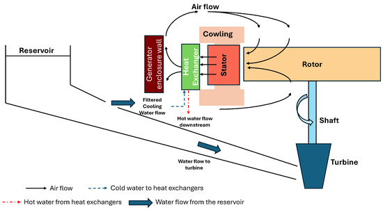
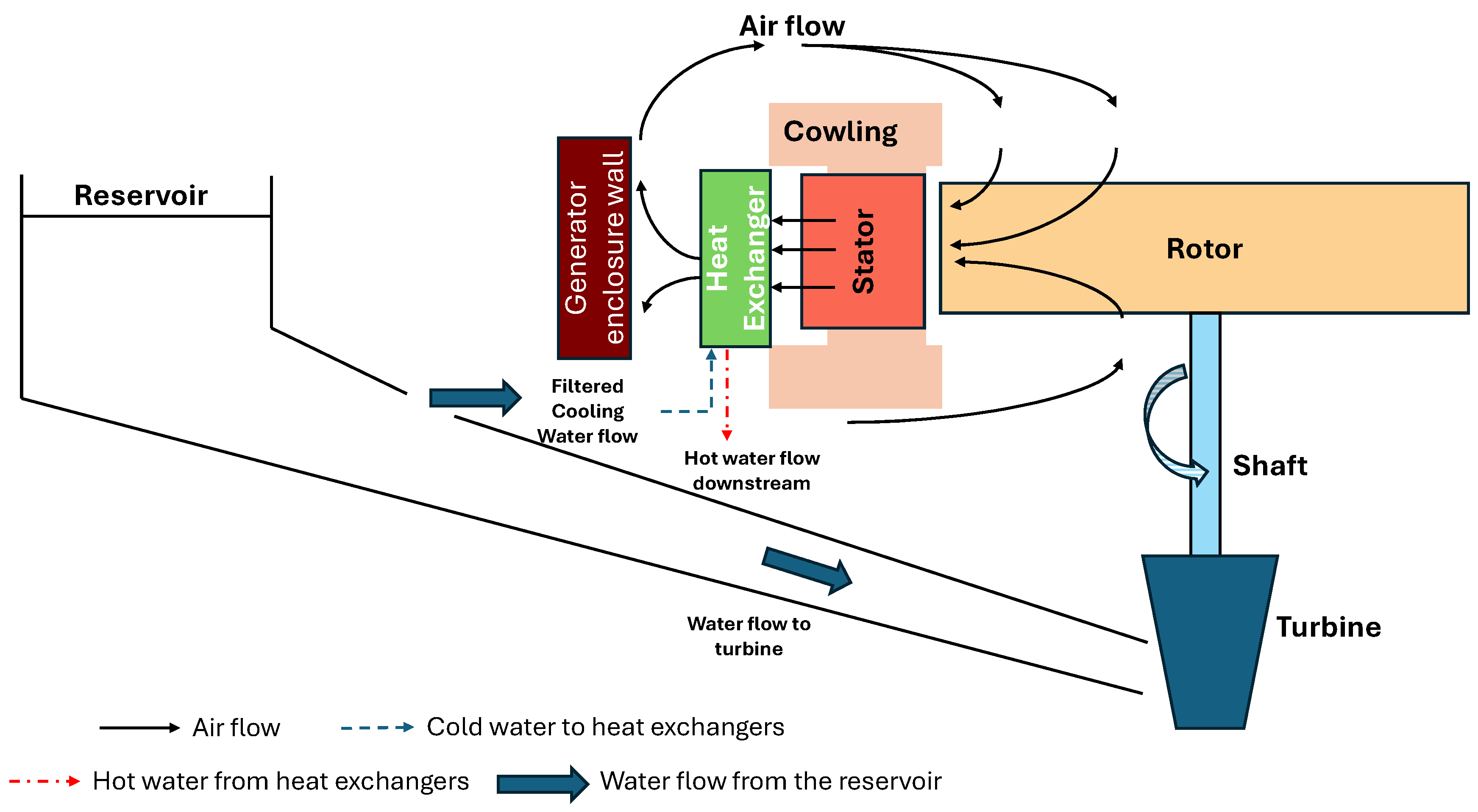
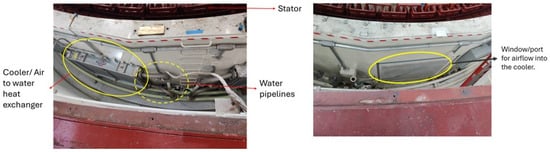
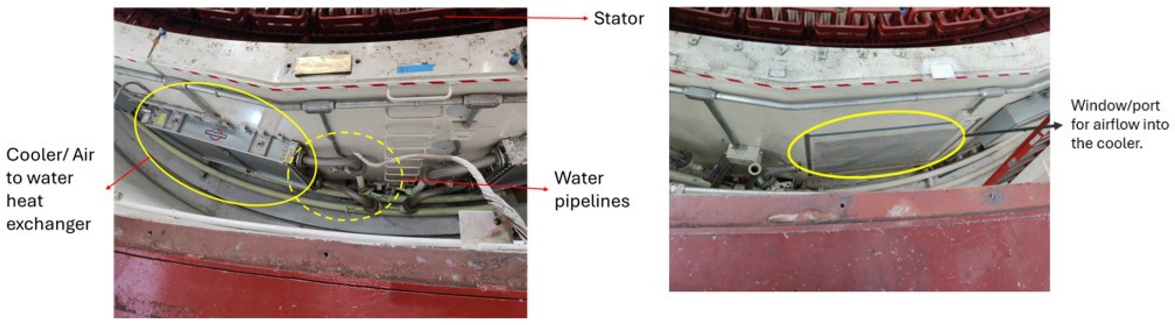
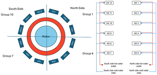
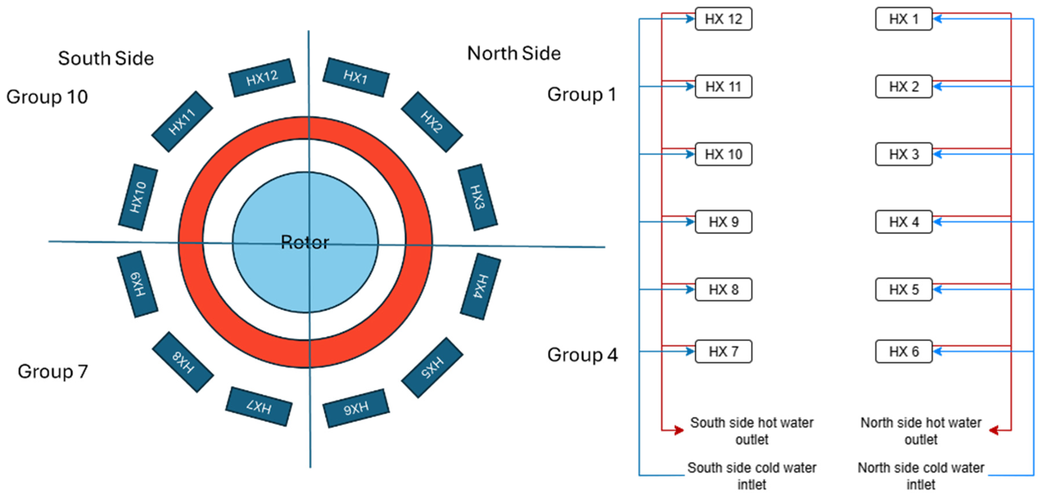
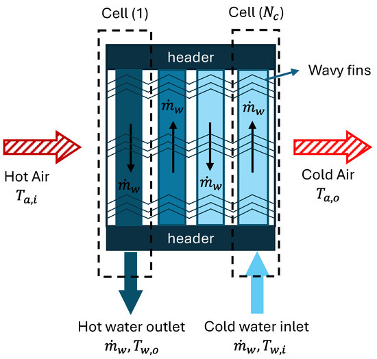
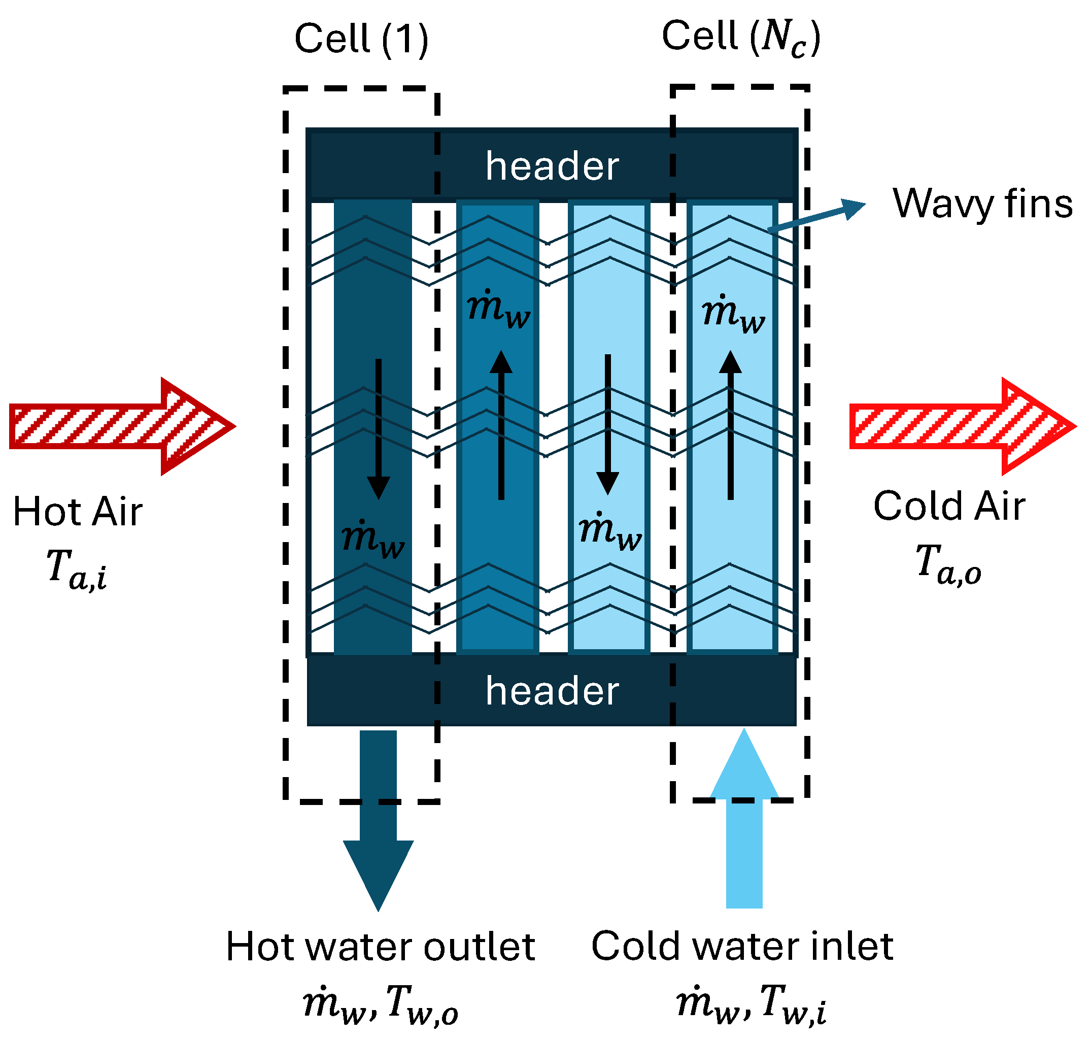
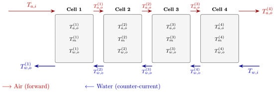
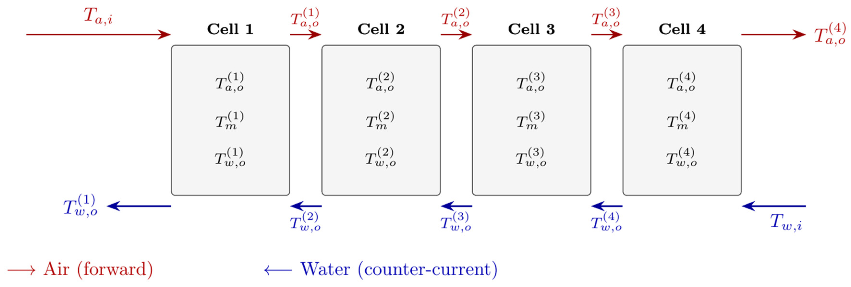
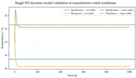
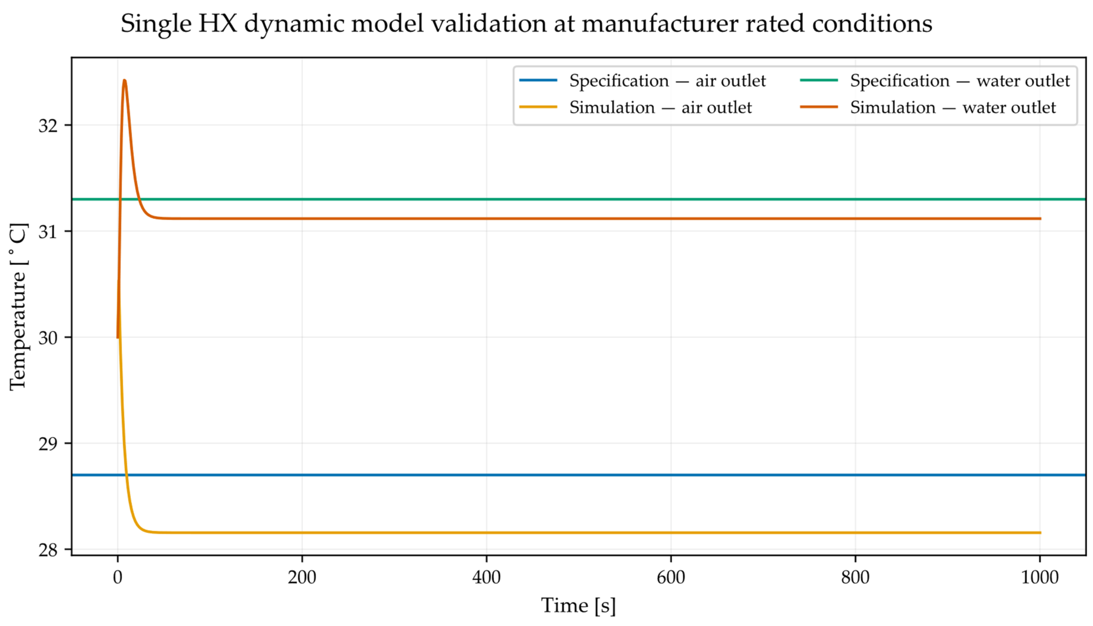
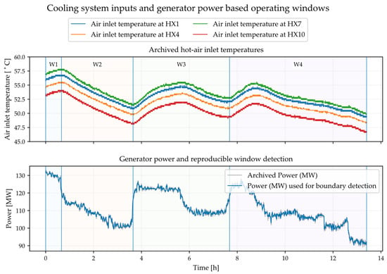
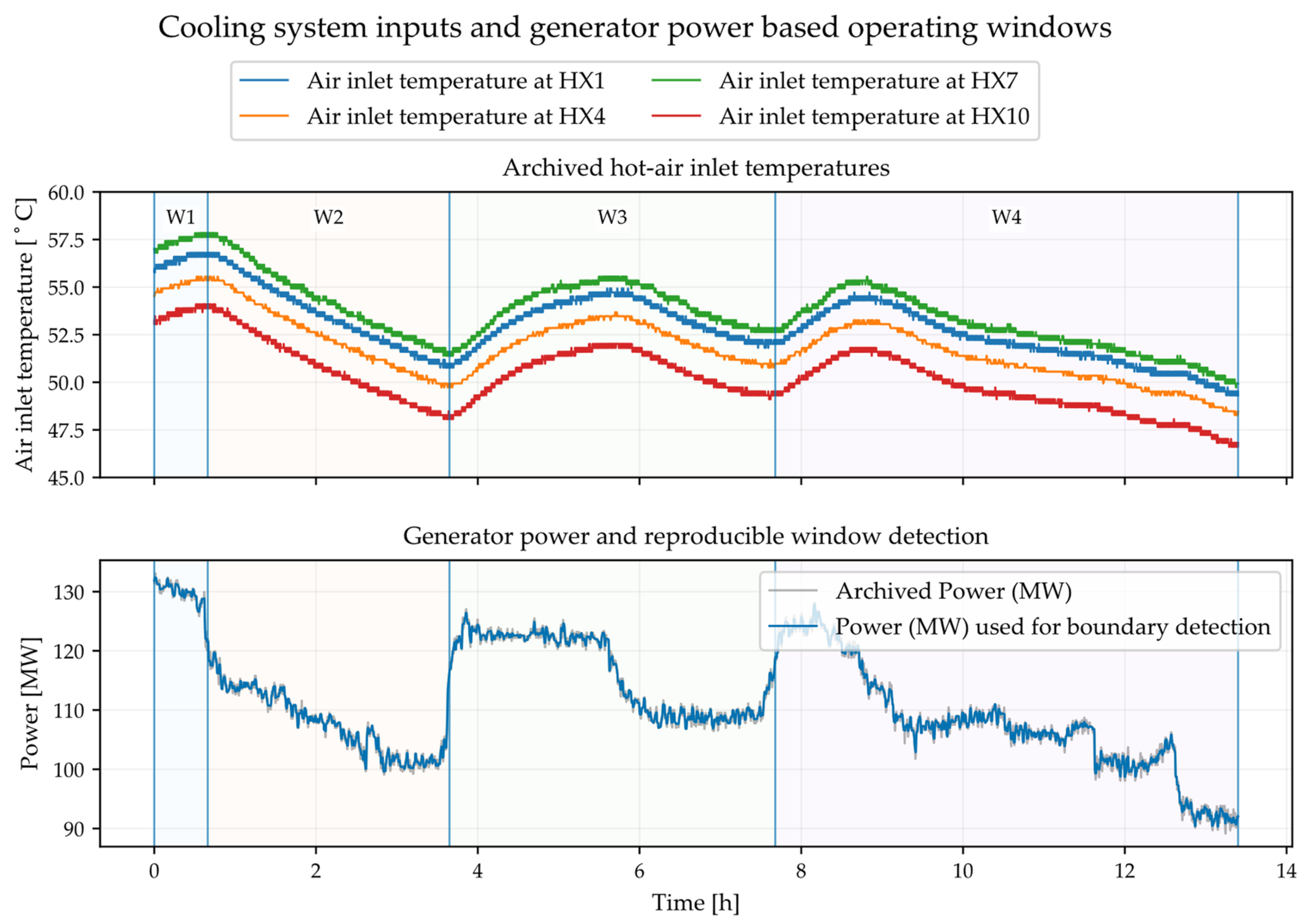
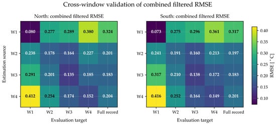
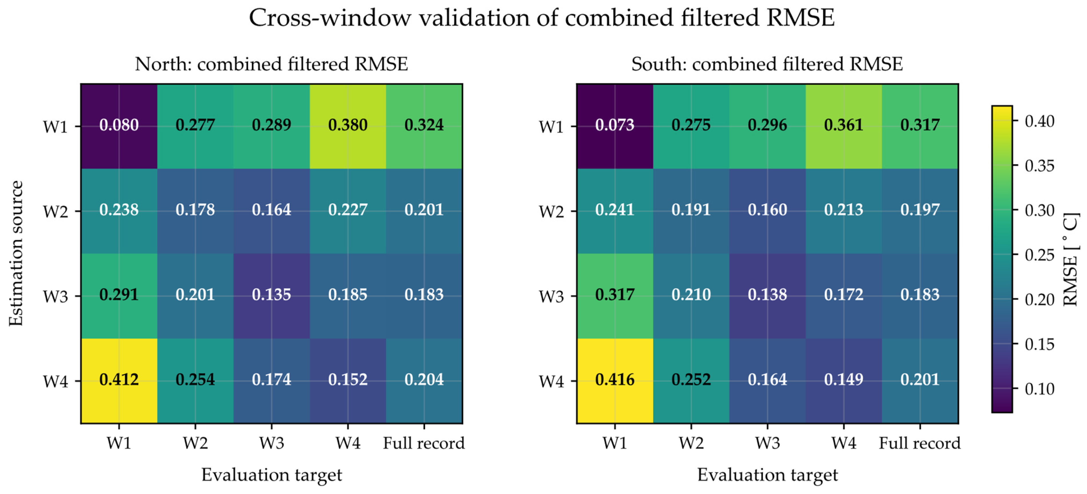
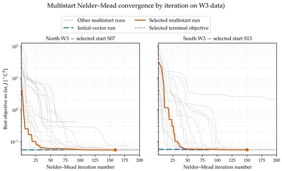
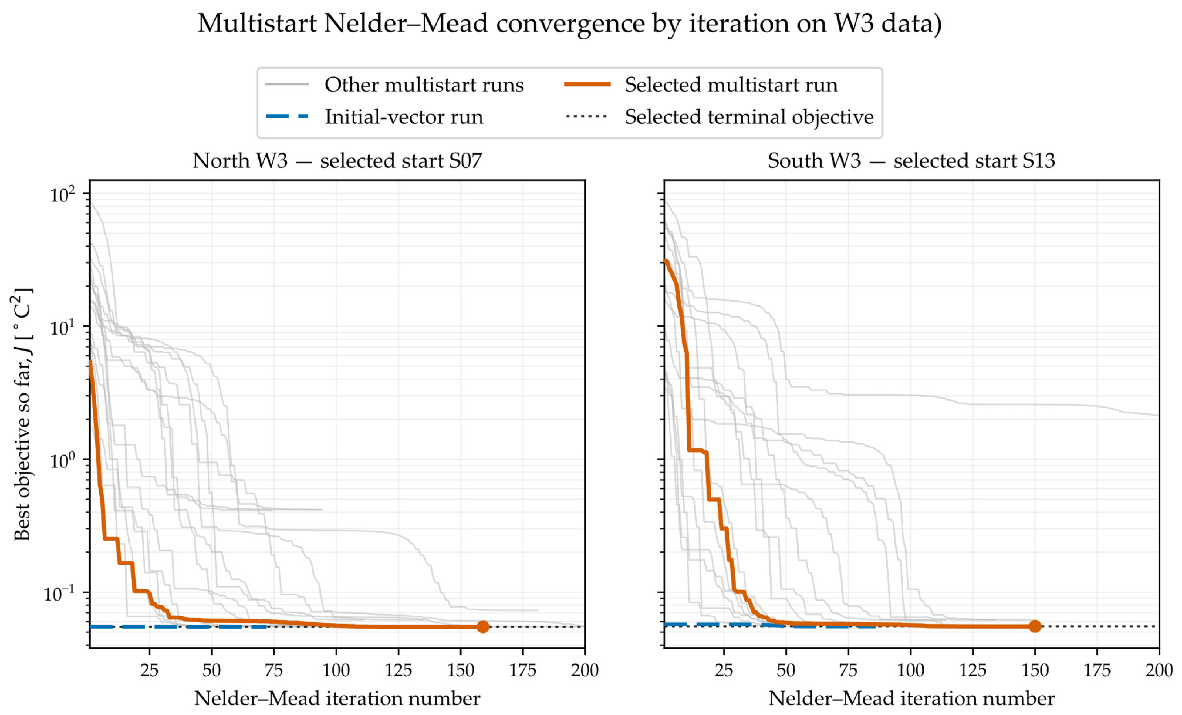
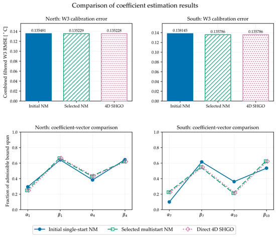
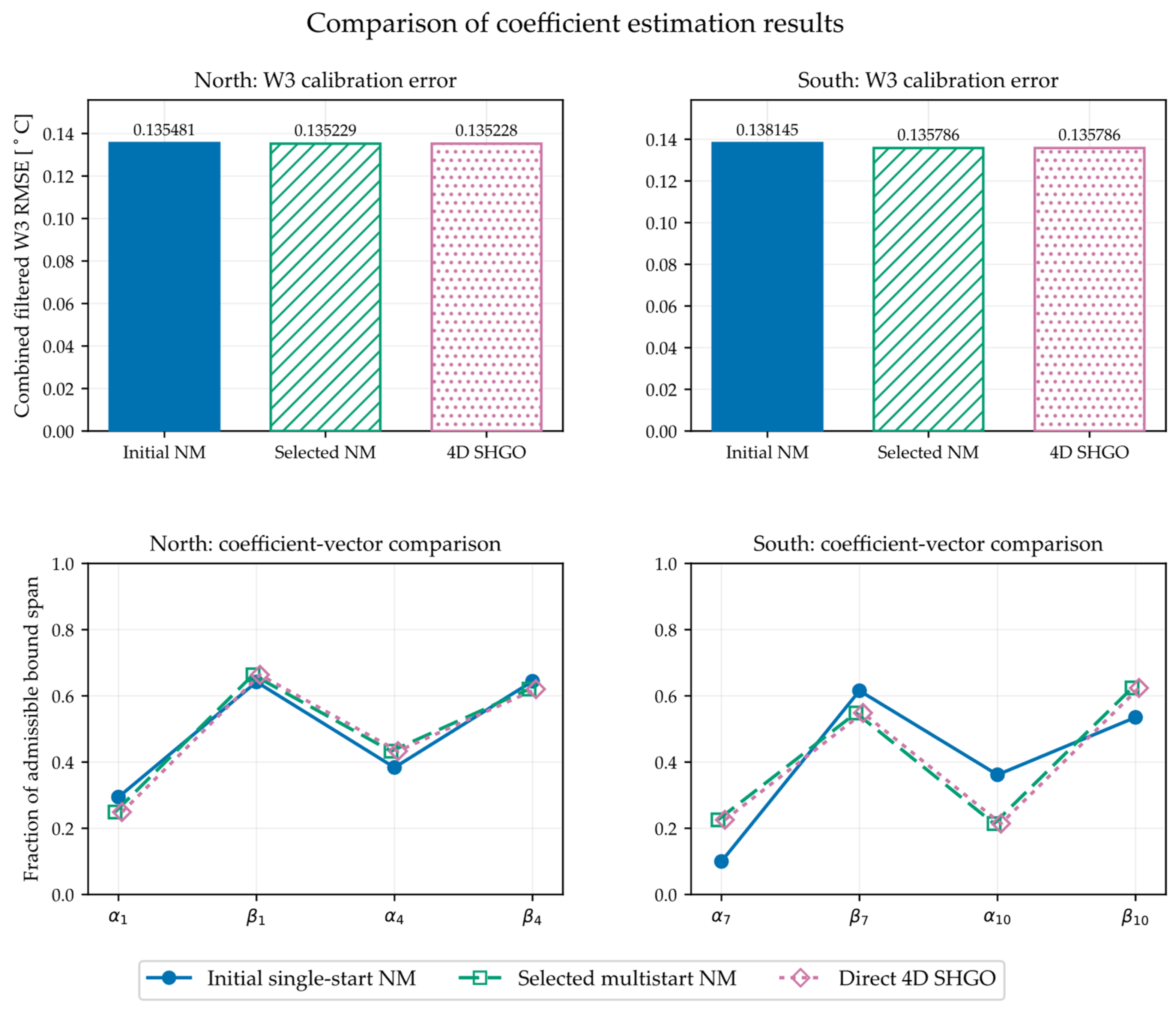
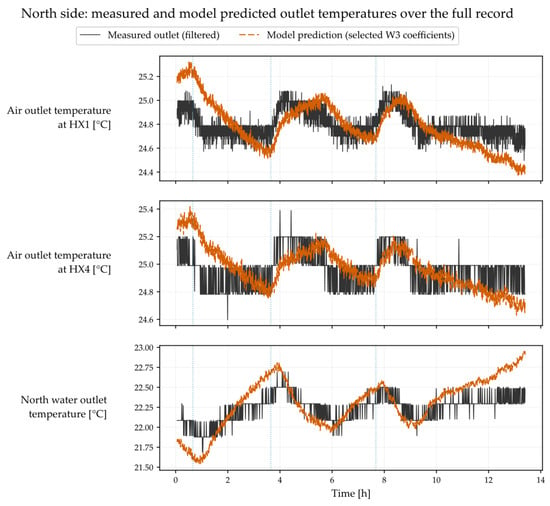
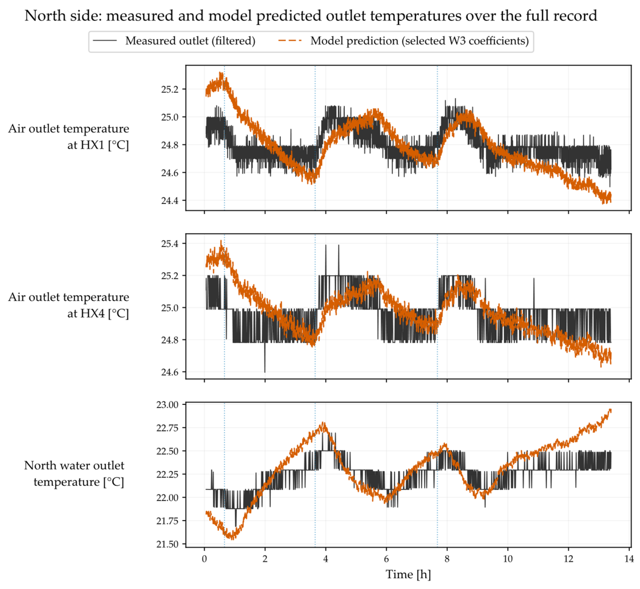
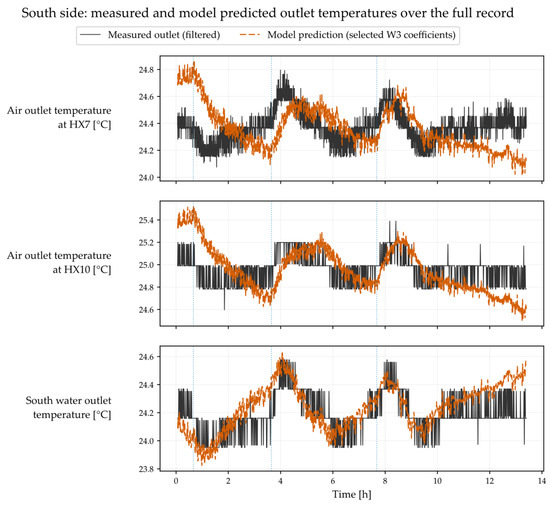
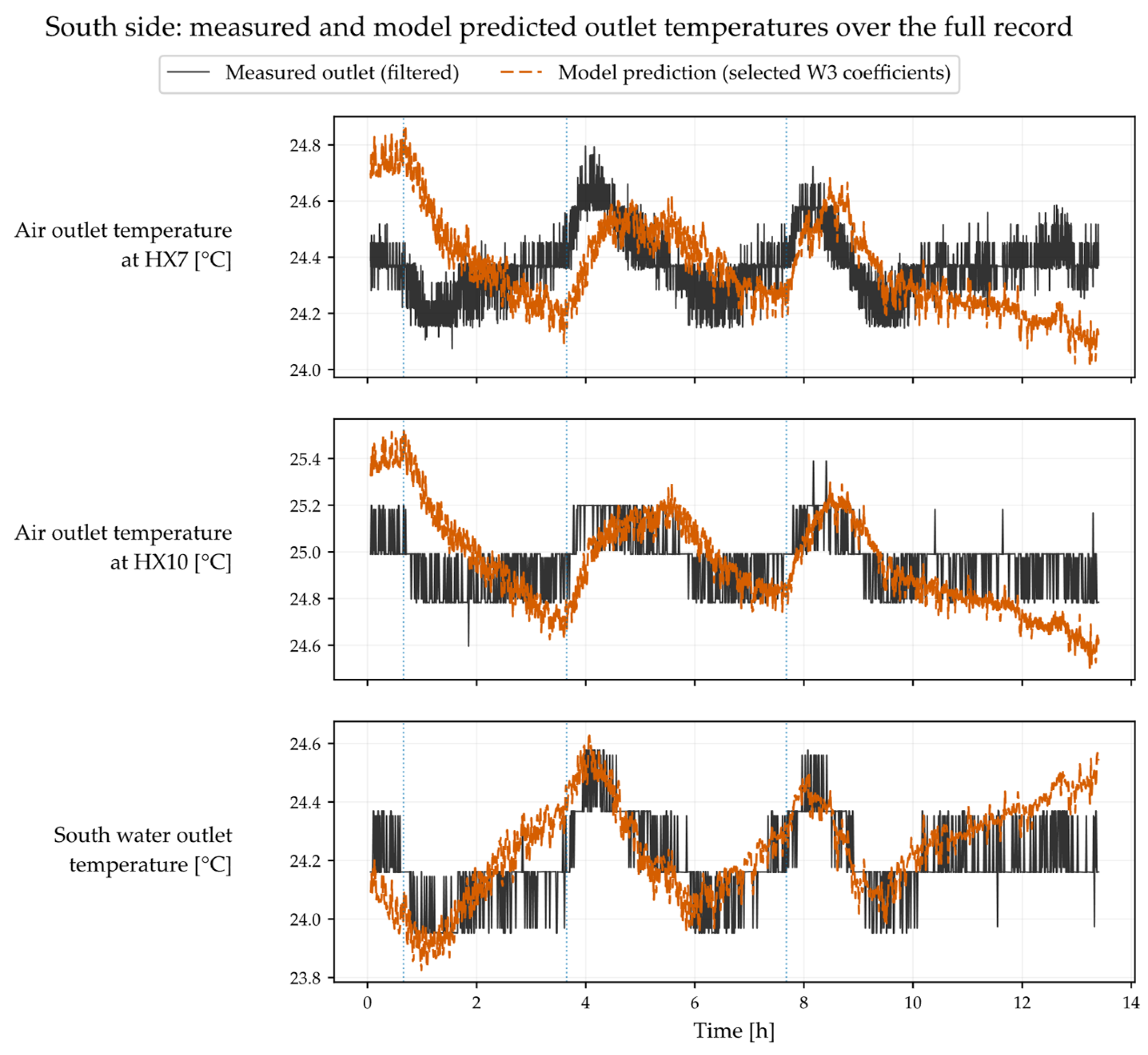
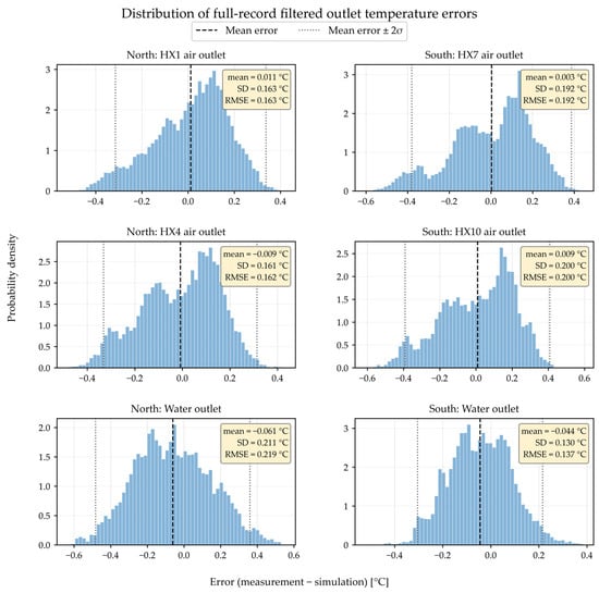
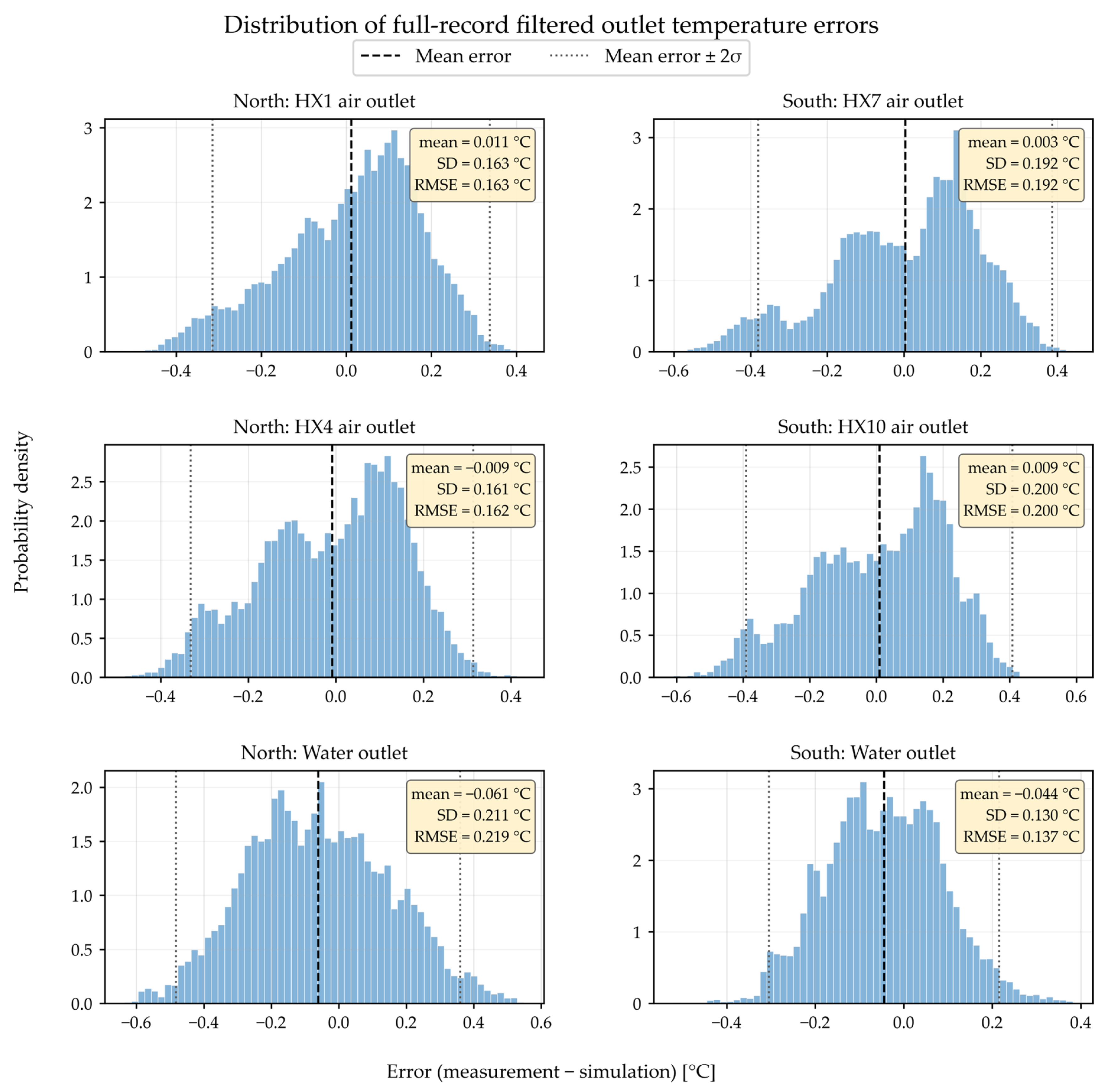
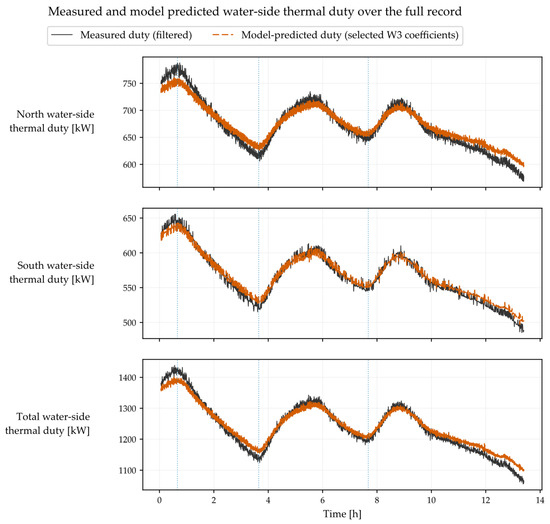
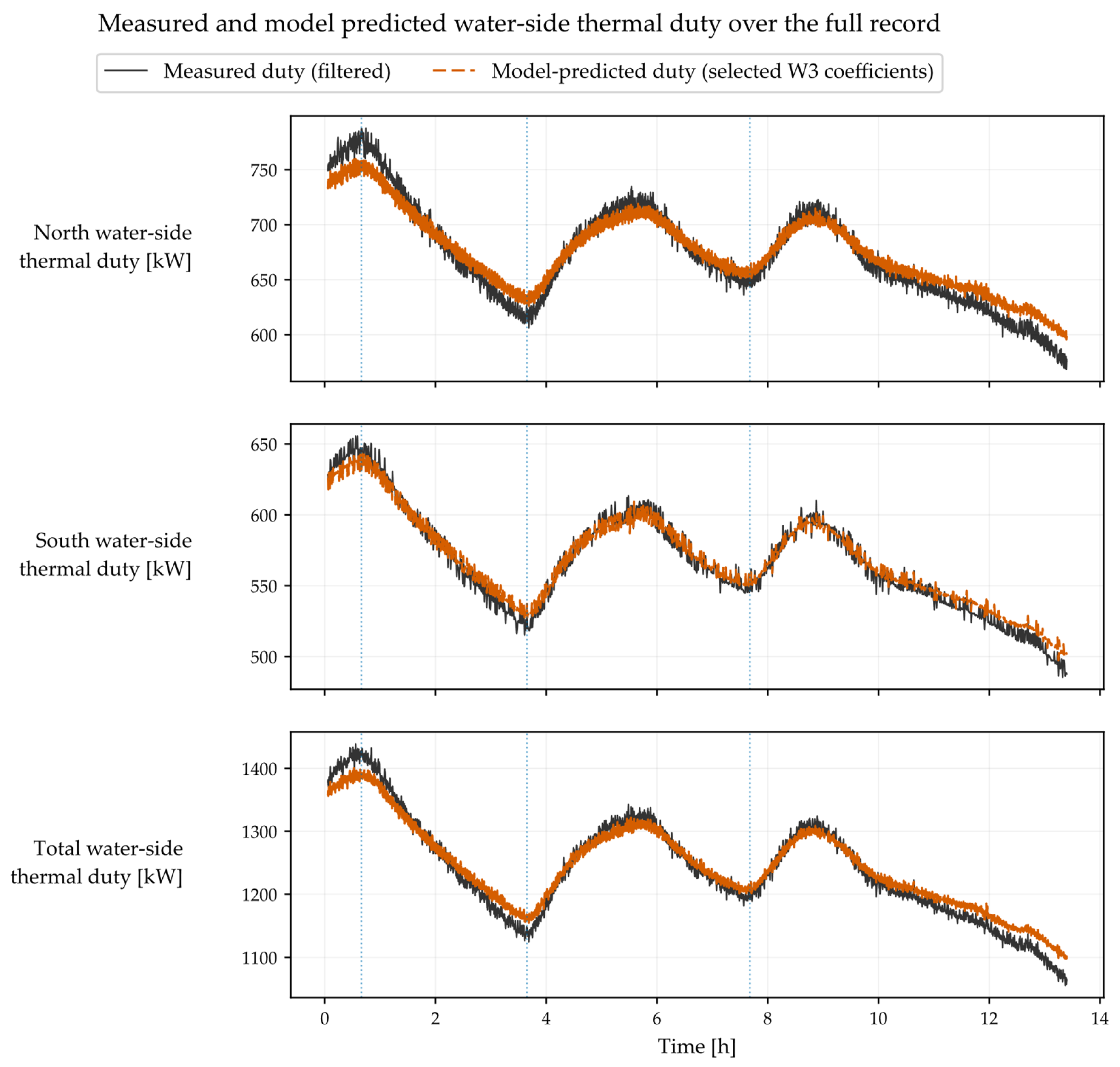

Disclaimer/Publisher’s Note: The statements, opinions and data contained in all publications are solely those of the individual author(s) and contributor(s) and not of MDPI and/or the editor(s). MDPI and/or the editor(s) disclaim responsibility for any injury to people or property resulting from any ideas, methods, instructions or products referred to in the content. |
© 2026 by the authors. Licensee MDPI, Basel, Switzerland. This article is an open access article distributed under the terms and conditions of the Creative Commons Attribution (CC BY) license.