A Novel Newmark Family of Fourth-Order Accurate Algorithms with Complex Sub-Steps for Structural Dynamics

Abstract

A new family of fourth-order accurate time integration schemes is developed by introducing two complex time sub-steps into the classical Newmark family of second-order algorithms. These sub-steps consist of a pair of complex conjugate numbers, enabling the triangularization of a complex-valued effective stiffness matrix. The proposed formulation can be easily implemented in existing codes with only minor modifications to the standard Newmark algorithm. The solution is composed of both real (physical) and imaginary components. The real component provides fourth-order accuracy even in the presence of external loads and physical damping, while the imaginary component offers additional insight into the distribution of numerical errors, an original feature not previously reported for implicit formulations. Compared to the classical Newmark method with a time-step size four times smaller, the proposed scheme exhibits significantly lower numerical dissipation and dispersion errors. Furthermore, the sub-step procedure extends the critical time step of conditionally stable members of the Newmark family by a factor of $\sqrt{3}$. The numerical analysis performed in the proposed time integration method, along with the results obtained for dynamic structural problems, including a complex three-dimensional (3D) application, clearly demonstrate that the method outperforms both Fung’s fourth-order complex scheme and the classical Newmark approach in terms of accuracy.

1. Introduction

The importance of dynamic problems lies in the fact that most structures and engineering systems are subjected to time-dependent loads, such as vibrations, impacts, seismic excitations, and periodic forces [1]. Dynamic analysis is inherently tied to the physical nature of the problem, which may be classified based on its dominant frequency spectrum. Inertial problems are those governed by low-frequency modes (e.g., structural dynamics), while wave propagation problems are also dominated by high-frequency components (e.g., impact or shock loading). These problems are typically solved using numerical approximation methods in practical engineering applications [2,3,4]. While the Finite Element Method (FEM) remains the predominant approach for spatial discretization, direct time integration is the standard choice for the time discretization, which can be implemented in an explicit or implicit form. For inertial problems, implicit algorithms are often favored because many of them are unconditionally stable, allowing the use of large time steps. In contrast, for wave propagation problems that require small time steps, explicit approaches become competitive due to their lower computational cost per time step [2,3].

Since spatial discretizations introduce spurious high-frequency artifacts into the numerical solution, time integration methods are often designed to suppress nonphysical oscillations via numerical (algorithmic) damping. The importance of the numerical damping also varies by application. For inertial problems, where the goal is to accurately capture the low-frequency response, excessive algorithmic dissipation should be avoided to allow the use of large time steps. Although these algorithms are designed to minimize the effects on lower-frequency modes, non-dissipative schemes frequently yield higher amplitude and period accuracy than their dissipative counterparts, mainly for long-duration time-history analyses. On the other hand, in some wave propagation problems, the nonphysical oscillations may compromise the solution; therefore, the numerical damping can be activated to mitigate such spurious oscillations. For this reason, algorithms with controllable numerical damping can handle a wider range of applications in a unified way. Despite the advancement of schemes that enable parametric control of high-frequency dissipation preserving low-frequency accuracy (e.g., HHT [5], generalized-$\alpha$ [6], ImGA- and ExGA-Newmark [1,7], ${\rho }_{\infty }$-Bathe [8,9] and Soares methods [10]), the classic Newmark [11] with the trapezoidal rule (constant average acceleration) still remains popular throughout industry and academia, especially in problems where an accurate integration of the relevant physical frequencies is prioritized over filtering out inaccurate high-frequency components. This enduring popularity stems from its capability to provide reliable solutions while preserving energy, a property of great importance for numerous linear as well as nonlinear vibration and structural dynamic problems [12,13,14,15] and for the efficient use of large time steps.

Owing to the significant advances of higher order spatial discretization techniques such as spectral element methods [16] and isogeometric methods [17,18] that yield distinct and advantageous numerical features, the pursuit for highly accurate dynamic response also in the time-domain analysis, combined with the need for computational efficiency and compatibility with the spatial discretization, has also motivated the development of high-order time-integration methods. One approach, which is also the focus of this paper, for increasing the order of accuracy in time-stepping schemes involves the use of time sub-steps. From the literature review and considering the Newmark method, we can mention the three real sub-steps proposed by Tarnow and Simo [19] that allow fourth-order algorithms to be constructed from second-order ones. Later on, Fung [20,21,22,23,24] developed some high-order implicit methods, the main idea is to combine linearly the solutions of the Newmark method evaluated at specific sub-steps. The author noted, however, that certain classes of loading needed to be modified to maintain the load-operator accuracy order consistent with that of the amplification matrix. In fact, a fundamental challenge in developing high-order time integration schemes is ensuring that the order of accuracy of the load operator is mathematically compatible with that of the amplification matrix, a classical issue highlighted in the literature by Wood [25]. Along these lines, Fung demonstrated that using two complex sub-steps yields third-order accuracy with numerical dissipation or fourth-order accuracy without numerical dissipation both with significantly smaller errors than those obtained using real sub-steps. Formulations based on the Newmark method are often reported in the literature indicating its continued relevance in science and engineering. In this context, a recent advancement was recently reported by Takács and Fülöp [26], who used backward analysis to incorporate two compensation strategies into the Newmark method, one that removes the numerical damping and another that attains fourth-order accuracy using the linear acceleration scheme.

Beyond the direct application of the Newmark method, the development of sub-stepping techniques to derive high-order algorithms also remains an active and growing area of research. Some recently proposed high-order implicit methods that use s sub-steps fall into the following two categories: sth-order accurate schemes with controllable numerical damping [27,28,29,30,31] or $(s+1)$th-order accurate schemes without controllable numerical damping [28,30,31,32]. For instance, Li et al. [28] developed three sub-step implicit algorithms, all of which adopt the average acceleration scheme (zero dissipation) for the first sub-step. A key distinction among these methods is that while the second- and third-order schemes exhibit controllable numerical dissipation, the fourth-order scheme lacks the dissipation control (achieving only moderate numerical damping) to attain such an accuracy order. In the method proposed by Song and Zhang [31], an efficient algorithm was developed when the implicit equation for a sub-step is in the same form as that of the trapezoidal method. The authors demonstrated that $(s+1)$th-order schemes also lack controlled numerical damping. Furthermore, modern methods seek to preserve the same order of accuracy of the amplification matrix in the load operator for forced responses [29,31,33,34]. We can mention the work of Lee and Noh [33], in which the external force is modeled at the last sub-step to ensure that the high-order accuracy is maintained during forced vibrations. Remarkably, the method achieves $(s+1)$th-order of accuracy using s sub-steps (for $s\le 5$) with spectral radius control.

High-order methods that utilize complex-valued systems have also been the focus of recent investigations. Song et al. [30] applied partial fraction to Padé expansions of order $(M,M)$ to achieve time-stepping schemes of order $2M$. The resulting equations are similar to the ones of the classical Newmark method but in the complex domain. When M is odd, the method solves one system with a real matrix and $(M-1)/2$ systems with complex matrices to advance a time step, whereas for even M, $M/2$ complex systems are solved. Later, Song et al. [35] extended the scheme to include controllable numerical dissipation by mixing the diagonal Padé expansion of order $(M,M)$ with the sub-diagonal Padé expansion of order $(M-1,M)$. However, this introduction of numerical damping limits the accuracy order to $2M-1$ in contrast to $2M$ in the previous approach. More recently, Song and Zhang [31] further advanced the method to design high-order composite schemes that utilize the same effective stiffness matrix in all sub-steps. They proposed schemes achieving sth- and $(s+1)$th-order of accuracy with s sub-steps. The authors observed that the second-order variant of this method is numerically equivalent to the ${\rho }_{\infty }$-Bathe method [8,9].

Motivated by the goal of developing a simple in terms of implementation yet robust high-order implicit algorithm, this paper presents a family of fourth-order accurate time integration methods based on the classical Newmark method for solving structural dynamic problems, employing two complex sub-steps. The proposed methodology simultaneously increases the order of accuracy and spectral stability of second-order algorithms of the Newmark family, addressing the general case that includes forced responses and physical damping. The family includes the classical average acceleration, linear acceleration, Fox Goodwing and all other numerical non-dissipative members of the Newmark family, preserving fourth-order accuracy also in forced problems with physical damping. Furthermore, our sub-steps yield a complex solution, a distinct property whose advantages were first discussed in Souza et al. [36]. It is noteworthy that the fourth-order accurate central difference method (CD²) proposed in that work is a specific non-dissipative member of the broader family of methods presented herein. As commented at the beginning of the introduction, the algorithms of the Newmark family, though widely used, cannot introduce dissipation while maintaining second-order accuracy. In a similar way, the proposed family of fourth-order accurate schemes is also designed to be non-dissipative, focusing on the accurate solution of inertial problems with long periods of time that are common in a great deal of structural engineering applications.

The remainder of the paper is as follows. Section 2 briefly revisits the Newmark formulation for solving the equations of motion raised in structural dynamics. In Section 3 we present the novel high-order family of methods. In Section 4 numerical examples that validate the method are analyzed. Finally, conclusions are drawn in Section 5, summarizing the main findings and outlining directions for future research.

2. Newmark Family for Structural Dynamics

The general form of equations of motion encountered in linear structural dynamics, assuming the time domain of analysis $I=(0,t_f]\subset {\mathbb{R}}^{+}$, can be stated, in matrix form, as given ${\mathbf{U}}^0\in {\mathbb{R}}^N$, ${\dot{\mathbf{U}}}^0\in {\mathbb{R}}^N$ (vectors of initial conditions) and $\mathbf{F}:I\to {\mathbb{R}}^N$ (load vector), find $\mathbf{U}:I\to {\mathbb{R}}^N$ such that

$$\begin{array}{cc}\hfill & \mathbf{M}\ddot{\mathbf{U}}\left(t\right)+\mathbf{C}\dot{\mathbf{U}}\left(t\right)+\mathbf{KU}\left(t\right)=\mathbf{F}\left(t\right)\hfill \end{array}$$

(1)

$$\begin{array}{cc}\hfill & \mathbf{U}\left(0\right)={\mathbf{U}}^0\hfill \end{array}$$

(2)

$$\begin{array}{cc}\hfill & \dot{\mathbf{U}}\left(0\right)={\dot{\mathbf{U}}}^0\hfill \end{array}$$

(3)

where $\mathbf{U},\dot{\mathbf{U}},\ddot{\mathbf{U}}:I\to {\mathbb{R}}^N$ are the displacement vector and its time derivatives, respectively. Moreover, $\mathbf{M},\mathbf{C},\mathbf{K}\in {\mathbb{R}}^{N\times N}$ are, respectively, the mass, damping and stiffness matrices with N being the total number of unknown degrees of freedom [2,3,4,37].

The solution of Equations (1)–(3) can be performed by the so-called time integration methods in which the time domain of analysis I is partitioned into a set of n time intervals, i.e., $I={\displaystyle \bigcup _{k=0}^{n-1}}\left[t_k,t_{k+1}\right]$ with $0=t_0<t_1<\dots <t_n=t_f$ and a time-step length $\Delta t=t_{k+1}-t_k$ (not necessarily equal over the time steps) for which the solution is computed by suitable approximations. Among the various existing time integration methods, the most renowned for structural dynamics is the Newmark family of time integration algorithms. The Newmark family is widely used in both industry, through commercial simulation software, and academia to discretize Equation (1), and it can be concisely derived by evaluating Equation (1) at the current time instant $t_{k+1}$ and utilizing the Taylor series expansions of the displacement and velocity vectors about the time instant $t_k$ for which the solution vectors are known, resulting in [3,4,37,38]:

$$\begin{array}{cc}\hfill & \mathbf{M}{\ddot{\mathbf{U}}}^{k+1}+\mathbf{C}{\dot{\mathbf{U}}}^{k+1}+\mathbf{K}{\mathbf{U}}^{k+1}={\mathbf{F}}^{k+1}\hfill \end{array}$$

(4)

$$\begin{array}{cc}\hfill & {\mathbf{U}}^{k+1}={\mathbf{U}}^k+\Delta t{\dot{\mathbf{U}}}^k+{\displaystyle \underset{t_k}{\overset{t_{k+1}}{\int }}}\left(t_{k+1}-\tau \right)\ddot{\mathbf{U}}\left(\tau \right)d\tau \hfill \end{array}$$

(5)

$$\begin{array}{cc}\hfill & {\dot{\mathbf{U}}}^{k+1}={\dot{\mathbf{U}}}^k+{\displaystyle \underset{t_k}{\overset{t_{k+1}}{\int }}}\ddot{\mathbf{U}}\left(\tau \right)d\tau \hfill \end{array}$$

(6)

in which the aforementioned integrals, which are the remainders of the Taylor series expansions, are approximated according to Equations (7) and (8) after assuming a variation for the acceleration.

$$\begin{array}{cc}\hfill & {\displaystyle \underset{t_k}{\overset{t_{k+1}}{\int }}}\left(t_{k+1}-\tau \right)\ddot{\mathbf{U}}\left(\tau \right)d\tau \approx \left({\displaystyle \frac{1}{2}}-\beta \right)\Delta t^2{\ddot{\mathbf{U}}}^k+\beta \Delta t^2{\ddot{\mathbf{U}}}^{k+1}\hfill \end{array}$$

(7)

$$\begin{array}{cc}\hfill & {\displaystyle \underset{t_k}{\overset{t_{k+1}}{\int }}}\ddot{\mathbf{U}}\left(\tau \right)d\tau \approx \left(1-\gamma \right)\Delta t{\ddot{\mathbf{U}}}^k+\gamma \Delta t{\ddot{\mathbf{U}}}^{k+1}\hfill \end{array}$$

(8)

where parameters $\gamma$ and $\beta$ govern the assumed variation of the acceleration over the time interval and play a crucial role in controlling the stability and accuracy of the methods [3,37]. Throughout the text, the notation ${\mathbf{U}}^k\equiv \mathbf{U}\left(t_k\right)$, ${\mathbf{U}}^{k+1}\equiv \mathbf{U}\left(t_k+\Delta t\right)$, and so forth is systematically adopted for representing both numerical and analytical counterparts.

3. Proposed Time-Stepping Methods

A sub-stepping procedure can be employed to construct high-order methods based on the second-order schemes of the Newmark family. Here, the key idea of the proposed formulation as presented by Souza et al. [36] is to split the time-step length $\Delta t$ into two time sub-steps given by ${\theta }_1\Delta t$ and ${\theta }_2\Delta t$ such that ${\theta }_1\Delta t+{\theta }_2\Delta t=\Delta t$. In the first sub-step, the displacement, velocity, and acceleration vectors are computed at time $t_k+{\theta }_1\Delta t$ from the previous known solution at time $t_k$ by applying the Newmark method (Equations (4)–(8)) with a time-step size of ${\theta }_1\Delta t$, as follows:

$$\begin{array}{cc}\hfill & \mathbf{M}{\ddot{\mathbf{U}}}^{k+{\theta }_1}+\mathbf{C}{\dot{\mathbf{U}}}^{k+{\theta }_1}+\mathbf{K}{\mathbf{U}}^{k+{\theta }_1}={\mathbf{F}}^{k+{\theta }_1}\hfill \end{array}$$

(9)

$$\begin{array}{cc}\hfill & {\mathbf{U}}^{k+{\theta }_1}={\mathbf{U}}^k+{\theta }_1\Delta t{\dot{\mathbf{U}}}^k+{\left({\theta }_1\Delta t\right)}^2\left[\left({\displaystyle \frac{1}{2}}-\beta \right){\ddot{\mathbf{U}}}^k+\beta {\ddot{\mathbf{U}}}^{k+{\theta }_1}\right]\hfill \end{array}$$

(10)

$$\begin{array}{cc}\hfill & {\dot{\mathbf{U}}}^{k+{\theta }_1}={\dot{\mathbf{U}}}^k+\left({\theta }_1\Delta t\right)\left[\left(1-\gamma \right){\ddot{\mathbf{U}}}^k+\gamma {\ddot{\mathbf{U}}}^{k+{\theta }_1}\right]\hfill \end{array}$$

(11)

In the second sub-step, the solution is advanced from $t_k+{\theta }_1\Delta t$ to $t_k+\Delta t$ with a time-step size of ${\theta }_2\Delta t$, once again employing the Newmark method, yielding the desired solution at the end of the time step $\Delta t$:

$$\begin{array}{cc}\hfill & \mathbf{M}{\ddot{\mathbf{U}}}^{k+1}+\mathbf{C}{\dot{\mathbf{U}}}^{k+1}+\mathbf{K}{\mathbf{U}}^{k+1}={\mathbf{F}}^{k+1}\hfill \end{array}$$

(12)

$$\begin{array}{cc}\hfill & {\mathbf{U}}^{k+1}={\mathbf{U}}^{k+{\theta }_1}+{\theta }_2\Delta t{\dot{\mathbf{U}}}^{k+{\theta }_1}+{\left({\theta }_2\Delta t\right)}^2\left[\left({\displaystyle \frac{1}{2}}-\beta \right){\ddot{\mathbf{U}}}^{k+{\theta }_1}+\beta {\ddot{\mathbf{U}}}^{k+1}\right]\hfill \end{array}$$

(13)

$$\begin{array}{cc}\hfill & {\dot{\mathbf{U}}}^{k+1}={\dot{\mathbf{U}}}^{k+{\theta }_1}+\left({\theta }_2\Delta t\right)\left[\left(1-\gamma \right){\ddot{\mathbf{U}}}^{k+{\theta }_1}+\gamma {\ddot{\mathbf{U}}}^{k+1}\right]\hfill \end{array}$$

(14)

The determination of ${\theta }_1$ and ${\theta }_2$ required to obtain fourth-order accuracy is presented in details in Section 3.2. The other sub-stepping procedures based also on the Newmark method mentioned in the Section 1 to develop high-order time integration methods are briefly described here for comparison purposes (only fourth-order accurate schemes are considered). For instance, the sub-steps of Tarnow and Simo [19] (Figure 1a) can be applied to the Newmark family to achieve fourth-order accuracy; however, the critical time step for the classical Central Difference method (i.e., $\gamma =1/2$ and $\beta =0$) is reduced as described in Souza et al. [36]. On the other hand, instead of computing the sub-steps sequentially at the time instants $t_{k+{\theta }_1}$, $t_{k+{\theta }_1+{\theta }_2}$ and $t_{k+{\theta }_1+{\theta }_2+{\theta }_3}$ as the Tarnow and Simo procedure, Fung’s sub-stepping procedure [20] (Figure 1b) consists of linearly combining the solutions at the three time instants $t_{k+{\theta }_1}$, $t_{k+{\theta }_2}$ and $t_{k+{\theta }_3}$, allowing the solution of each sub-step to be compute simultaneously. However, it does not directly assure fourth-order accuracy for a general load case and requires modifying the load function by first approximating it as a polynomial by then applying a correction in the cubic term. Conversely, in this paper, we propose a more direct and straightforward approach as sketched in Figure 1c (using the implicit Newmark method) which preserves the order of accuracy in forced responses without any type of modification into the load function. This approach was previously investigated with the explicit Central Difference (CD) method [36], where the proposed approach increased the critical time step by 73% and achieved computational efficiency and numerical accuracy comparable to the most efficient fourth-order methods reported in the literature.

Figure 1. Schematic representation of some sub-steps for achieving fourth-order accuracy in the Newmark time integration method: (a) Tarnow and Simo [19], (b) Fung [20], and (c) proposed sub-steps.

3.1. Single Degree of Freedom

To investigate and compare the numerical properties of the proposed time integration method, we apply the modal decomposition procedure [2,3] by using the modal transformation $\mathbf{U}\left(t\right)=\mathbf{\Phi }\mathbf{u}\left(t\right)$ with $\mathbf{\Phi }\in {\mathbb{R}}^{N\times N}$ being the undamped modal matrix whose columns are the eigenvectors, and $\mathbf{u}:I\to {\mathbb{R}}^N$ stands for the modal generalized displacement vector. The modal matrix is constructed such that the orthogonal properties ${\mathbf{\Phi }}^T\mathbf{K}\mathbf{\Phi }=\mathrm{diag}\left[{\omega }_1^2,\dots ,{\omega }_j^2,\dots ,{\omega }_N^2\right]$ and ${\mathbf{\Phi }}^T\mathbf{M}\mathbf{\Phi }=\mathbf{I}$ ($\mathbf{I}\in {\mathbb{R}}^{N\times N}$ stands for the identity matrix) are satisfied, in which ${\omega }_j$ is the $j_{th}$ natural frequency of the system. In this way, considering proportional damping, we can transform Equation (1) into a set of decoupled SDOF equations (modal equations) of the following form (hereafter, to simplify the notation, the $j_{th}$ modal index is dropped):

$$\begin{array}{c}\hfill \ddot{u}\left(t\right)+2\xi \omega \dot{u}\left(t\right)+{\omega }^{2}u\left(t\right)=f\left(t\right)\end{array}$$

(15)

where $\xi \in [0,1)$ is the physical damping ratio, $\omega =2\pi /T$ with T being the natural period, $u:I\to \mathbb{R}$ is the generalized displacement, while $f:I\to \mathbb{R}$ is the load function that arises after the transformation.

In this way, it is sufficient to investigate the numerical properties of the time integration method by comparing the numerical solution with the analytical one of such a SDOF model. To this end, the displacement and velocity responses of the SDOF system can be obtained analytically using the Green’s function [39] according to the following expressions written in a step-by-step form [1]:

$$\left[\begin{array}{c}{u}^{k+1}\\ {\dot{u}}^{k+1}\end{array}\right]=\underset{\mathbf{A}\left(\Delta t\right)}{\underbrace{\left[\begin{array}{cc}\dot{g}\left(\Delta t\right)+2\xi \omega g\left(\Delta t\right)& g\left(\Delta t\right)\\ \ddot{g}\left(\Delta t\right)+2\xi \omega \dot{g}\left(\Delta t\right)& \dot{g}\left(\Delta t\right)\end{array}\right]}}\left[\begin{array}{c}{u}^k\\ {\dot{u}}^k\end{array}\right]+\underset{\mathbf{L}\left(\Delta t,t_k\right)}{\underbrace{\left[\begin{array}{c}{\displaystyle {\displaystyle \underset{0}{\overset{\Delta t}{\int }}}g\left(\Delta t-\tau \right)f\left(t_k+\tau \right)d\tau }\\ {\displaystyle {\displaystyle \underset{0}{\overset{\Delta t}{\int }}}\dot{g}\left(\Delta t-\tau \right)f\left(t_k+\tau \right)d\tau }\end{array}\right]}}$$

(16)

where $g\left(t\right)={\mathrm{e}}^{-\xi \omega t}{\displaystyle \frac{sin\left({\omega }_{d}t\right)}{{\omega }_d}}$ for $0\le \xi <1$ and ${\omega }_d=\omega \sqrt{1-{\xi }^2}$; besides, $\mathbf{A}\left(\Delta t\right)\in {\mathbb{R}}^{2\times 2}$ stands for the amplification matrix, and $\mathbf{L}\left(\Delta t,t_k\right)\in {\mathbb{R}}^2$ is the so-called load operator vector, which accounts for the particular solution (or forced response) through the convolution integrals.

Conversely, numerical counterparts of the amplification matrix and the load operator vector obtained by the Newmark method can be defined as [3]

$$\begin{array}{cc}\hfill {\mathbf{A}}_{\mathrm{N}}(\Delta t)& ={{\mathbf{A}}_1(\Delta t)}^{-1}{\mathbf{A}}_2(\Delta t)\hfill \end{array}$$

(17)

$$\begin{array}{cc}\hfill {\mathbf{L}}_{\mathrm{N}}(\Delta t,t_k)& ={{\mathbf{A}}_1(\Delta t)}^{-1}\left[\begin{array}{c}{\displaystyle \frac{\Delta t^2}{2}}\left((1-2\beta )f\left(t_k\right)+2\beta f(t_k+\Delta t)\right)\\ \Delta t\left((1-\gamma )f\left(t_k\right)+\gamma f(t_k+\Delta t)\right)\end{array}\right]\hfill \end{array}$$

(18)

where

$$\begin{array}{cc}\hfill {\mathbf{A}}_1(\Delta t)& =\left[\begin{array}{cc}1+\Delta t^2\beta {\omega }^2& 2\Delta t^2\beta \xi \omega \\ \Delta t\gamma {\omega }^2& 1+2\Delta t\gamma \xi \omega \end{array}\right]\hfill \end{array}$$

(19)

$$\begin{array}{cc}\hfill {\mathbf{A}}_2(\Delta t)& =\left[\begin{array}{cc}1-{\displaystyle \frac{\Delta t^2}{2}}(1-2\beta ){\omega }^2& \Delta t(1-\Delta t(1-2\beta \left)\xi \omega \right)\\ -\Delta t(1-\gamma ){\omega }^2& 1-2\Delta t(1-\gamma )\xi \omega \end{array}\right]\hfill \end{array}$$

(20)

The amplification matrix and the load operator vector for the method proposed in this paper are written as follows (the superscript 2 of ${\mathrm{N}}^2$ refers to the use of two sub-steps in the Newmark method):

$$\begin{array}{cc}\hfill {\mathbf{A}}_{{\mathrm{N}}^2}(\Delta t)& ={\mathbf{A}}_{\mathrm{N}}({\theta }_2\Delta t){\mathbf{A}}_{\mathrm{N}}({\theta }_1\Delta t)\hfill \end{array}$$

(21)

$$\begin{array}{cc}\hfill {\mathbf{L}}_{{\mathrm{N}}^2}(\Delta t,t_k)& ={\mathbf{A}}_{\mathrm{N}}({\theta }_2\Delta t){\mathbf{L}}_{\mathrm{N}}({\theta }_1\Delta t,t_k)+{\mathbf{L}}_{\mathrm{N}}({\theta }_2\Delta t,t_{k+{\theta }_1})\hfill \end{array}$$

(22)

where ${\mathbf{A}}_{\mathrm{N}}\left(·\right)\in {\mathbb{R}}^{2\times 2}$ and ${\mathbf{L}}_{\mathrm{N}}(·,·)\in {\mathbb{R}}^2$ are given by Equation (17) and Equation (18), respectively.

In addition to the classical Newmark method, for comparison purposes, we also consider the two complex sub-stepping procedure of Fung (Figure 1b) that combines linearly the solutions in the sub-steps [20] and the procedure of three real sub-steps of Tarnow and Simo [19] applied to the Newmark method to achieve fourth-order accuracy, which are called hereafter only as Fung method and Tarnow and Simo method, respectively. The amplification matrix and load operator vector of the Tarnow and Simo method [19] are given by

$$\begin{array}{cc}\hfill {\mathbf{A}}_{\mathrm{TS}}(\Delta t)& ={\mathbf{A}}_{\mathrm{N}}({\theta }_3\Delta t){\mathbf{A}}_{\mathrm{N}}({\theta }_2\Delta t){\mathbf{A}}_{\mathrm{N}}({\theta }_1\Delta t)\hfill \end{array}$$

(23)

$$\begin{array}{cc}\hfill {\mathbf{L}}_{\mathrm{TS}}(\Delta t,t_k)& ={\mathbf{A}}_{\mathrm{N}}({\theta }_3\Delta t){\mathbf{A}}_{\mathrm{N}}({\theta }_2\Delta t){\mathbf{L}}_{\mathrm{N}}({\Theta }_1\Delta t,t_k)+{\mathbf{A}}_{\mathrm{N}}({\theta }_3\Delta t){\mathbf{L}}_{\mathrm{N}}({\Theta }_2\Delta t,t_{k+{\Theta }_1})+\hfill \\ \hfill & {\mathbf{L}}_{\mathrm{N}}({\Theta }_3\Delta t,t_{k+{\Theta }_2})\hfill \end{array}$$

(24)

where ${\Theta }_j={\sum }_{i=1}^j{\theta }_i$ and ${\theta }_1={\theta }_3=\alpha$, ${\theta }_2=1-2\alpha$, with $\alpha =(2+2^{1/3}+2^{-1/3})$. Conversely, the amplification matrix and load operator vector of the Fung method [20] are written as

$$\begin{array}{cc}\hfill {\mathbf{A}}_{\mathrm{F}}(\Delta t)& ={\displaystyle \sum _{i=1}^3}{\alpha }_i\left[{\mathbf{A}}_{\mathrm{N}}({\theta }_i\Delta t)\right]\hfill \end{array}$$

(25)

$$\begin{array}{cc}\hfill {\mathbf{L}}_{\mathrm{F}}(\Delta t,t_k)& ={\displaystyle \sum _{i=1}^3}{\alpha }_i\left[{\mathbf{L}}_{\mathrm{N}}({\theta }_i\Delta t,t_k)\right]\hfill \end{array}$$

(26)

where ${\alpha }_i$ is the weight for the solution in the sub-step ${\theta }_i$. The Fung sub-steps that presented lower dispersion and dissipation measures assume the following complex values: ${\alpha }_1=1$, ${\alpha }_2=i\sqrt{3}$, ${\alpha }_3=-i\sqrt{3}$, ${\theta }_1=0$, ${\theta }_2=(3-i\sqrt{3})/6$, and ${\theta }_3=(3+i\sqrt{3})/6$ considering the Newmark parameters as $\gamma =1/2$ and $\beta =1/4$ (trapezoidal rule).

3.2. Requirements for Fourth-Order Accuracy

To ensure p-order accuracy globally, the difference between Taylor series expansions of the analytical and numerical amplification matrices as well as load operator vectors must be of order $\mathcal{O}(\Delta t^{p+1})$ locally. The analytical amplification matrix can be found in Equation (16) and the numerical amplification matrix with two sub-sequentially substeps of Equation (21) can be written as

$$\begin{array}{cc}\hfill {\mathbf{A}}_{{\mathrm{N}}^2}(\Delta t)& ={{\mathbf{A}}_1({\theta }_2\Delta t)}^{-1}{\mathbf{A}}_2({\theta }_2\Delta t){{\mathbf{A}}_1({\theta }_1\Delta t)}^{-1}{\mathbf{A}}_2({\theta }_1\Delta t)\hfill \end{array}$$

(27)

with ${\mathbf{A}}_1(\Delta t)$ and ${\mathbf{A}}_2(\Delta t)$ given in Equation (19) and Equation (20), respectively.

To simplify the demonstration, the first sub-step ${\theta }_1=\theta$ is used to rewrite the second one as ${\theta }_2=1-\theta$; besides, to reduce the complexity of expressions, $\xi =0$ is initially assumed and later generalized for any value of $\xi$. In this way, the difference between Taylor series expansions of the analytical amplification matrix (see Appendix A) and numerical one of the proposed approach (Equation (27)) for $\xi =0$ can be concisely written as

$$\begin{array}{c}\hfill \mathbf{A}(\Delta t)-{\mathbf{A}}_{{\mathrm{N}}^2}(\Delta t)=\left[\begin{array}{cc}0& 0\\ 0& r_2\left(\gamma ,\theta \right)\end{array}\right]{\displaystyle \frac{{\omega }^2\Delta t^2}{2!}}+\left[\begin{array}{cc}0& {\displaystyle \frac{r_{3,a}\left(\gamma ,\beta ,\theta \right)}{\omega }}\\ \omega r_{3,b}\left(\gamma ,\theta \right)& 0\end{array}\right]{\displaystyle \frac{{\omega }^3\Delta t^3}{3!}}+\\ \hfill \left[\begin{array}{cc}{r}_{4,a}\left(\gamma ,\beta ,\theta \right)& 0\\ 0& r_{4,b}\left(\gamma ,\beta ,\theta \right)\end{array}\right]{\displaystyle \frac{{\omega }^4\Delta t^4}{4!}}+\mathcal{O}(\Delta t^5)\end{array}$$

(28)

where the auxiliary functions $r_2\left(\gamma ,\theta \right)$, $r_{3,a}\left(\gamma ,\beta ,\theta \right)$, $r_{4,a}\left(\gamma ,\beta ,\theta \right)$, $r_{4,b}\left(\gamma ,\beta ,\theta \right)$ are introduced for conciseness and are given by

$$\begin{array}{cc}\hfill r_2\left(\gamma ,\theta \right)=& (2\gamma -1)\left(1+2\theta (\theta -1)\right)\hfill \end{array}$$

(29)

$$\begin{array}{cc}\hfill r_{3,a}\left(\gamma ,\beta ,\theta \right)=& 3\theta (1-\theta )\left(1+(2\gamma -1)\theta \right)+6\beta \left(1+3\theta (\theta -1)\right)-1\hfill \end{array}$$

(30)

$$\begin{array}{cc}\hfill r_{3,b}\left(\gamma ,\theta \right)=& 1+3(\theta -1){\theta }^2-3\gamma \left(1-\theta -{\theta }^2+2{\theta }^3\right)\hfill \end{array}$$

(31)

$$\begin{array}{cc}\hfill r_{4,a}\left(\gamma ,\beta ,\theta \right)=& 1+6(\theta -1){\theta }^2\left(1+(2\gamma -1)\theta \right)-12\beta \left(1-2\theta +2{\theta }^3\right)\hfill \end{array}$$

(32)

$$\begin{array}{cc}\hfill r_{4,b}\left(\gamma ,\beta ,\theta \right)=& 1-12\gamma \theta {(\theta -1)}^2\left(1+(2\gamma -1)\theta \right)\hfill \\ \hfill & -24\beta \left(\gamma -(\theta -1){\theta }^3+2\gamma \theta (\theta -1)\left(2+(\theta -1)\theta \right)\right)\hfill \end{array}$$

(33)

The method is second-order accurate if $r_2\left(\gamma ,\theta \right)=0$, and hence, the roots of such a polynomial equation lead to the following two possible solutions:

$$\begin{array}{cc}\hfill \gamma & ={\displaystyle \frac{1}{2}}\hfill \end{array}$$

(34)

$$\begin{array}{cc}\hfill \theta & ={\displaystyle \frac{1\pm i}{2}}\hfill \end{array}$$

(35)

Here, the first solution ($\gamma =1/2$) determines a possible value of the Newmark parameter, while the second solution ($\theta =(1\pm i)/2$) determines a possible value for the sub-steps required to attain second-oder accuracy. By substituting the first solution (Equation (34)) into Equations (30) and (31), and noting that the resulting polynomial $r_{3,b}\left(1/2,\theta \right)=-1/2\left(1+3\left(-1+\theta \right)\theta \right)$ depends solely on $\theta$ and $r_{3,a}\left(1/2,\beta ,\theta \right)=\left(-1+6\beta \right)\left(1+3\left(-1+\theta \right)\theta \right)$, the roots with respect to $\theta$ of the equations $r_{3,a}\left(1/2,\beta ,\theta \right)=0$ and $r_{3,b}\left(1/2,\theta \right)=0$ to ensure third-order accuracy are equal and can be readily computed, yielding

$$\theta ={\displaystyle \frac{3\pm i\sqrt{3}}{6}}$$

(36)

In this way, $\theta ={\displaystyle \frac{3\pm i\sqrt{3}}{6}}$ are the possible sub-steps for the first solution. Once all possible values for the sub-steps have been computed, one can proceed the demonstration with respect to the other parameters $\gamma$ and $\beta$ by analyzing the conditions which render the polynomial functions $r_2\left(\gamma ,\theta \right)$, $r_{3,a}\left(\gamma ,\beta ,\theta \right)$, $r_{3,b}\left(\gamma ,\theta \right)$, $r_{4,a}\left(\gamma ,\beta ,\theta \right)$ and $r_{4,b}\left(\gamma ,\beta ,\theta \right)$ identically zero at least for the real part, a sufficient condition to guarantee fourth-order accuracy for the real response. Therefore, for the first solution (Equations (34) and (36)), one obtains the following:

$$\begin{array}{c}{r}_2\left({\displaystyle \frac{1}{2}},{\displaystyle \frac{3\pm i\sqrt{3}}{6}}\right)=0\hfill \\ r_{3,a}\left({\displaystyle \frac{1}{2}},\beta ,{\displaystyle \frac{3\pm i\sqrt{3}}{6}}\right)=0\hfill \\ r_{3,b}\left({\displaystyle \frac{1}{2}},{\displaystyle \frac{3\pm i\sqrt{3}}{6}}\right)=0\hfill \\ r_{4,a}\left({\displaystyle \frac{1}{2}},\beta ,{\displaystyle \frac{3\pm i\sqrt{3}}{6}}\right)=\pm i{\displaystyle \frac{\left(-1+4\beta \right)}{\sqrt{3}}}\hfill \\ r_{4,b}\left({\displaystyle \frac{1}{2}},\beta ,{\displaystyle \frac{3\pm i\sqrt{3}}{6}}\right)=\pm i{\displaystyle \frac{\left(1-4\beta \right)}{\sqrt{3}}}\hfill \end{array}$$

(37)

Therefore, the conditions $r_{4,a}\left({\displaystyle \frac{1}{2}},\beta ,{\displaystyle \frac{3\pm i\sqrt{3}}{6}}\right)=0$ and $r_{4,b}\left({\displaystyle \frac{1}{2}},\beta ,{\displaystyle \frac{3\pm i\sqrt{3}}{6}}\right)=0$ are satisfied only when $\beta =1/4$. However, for any other real value of $\beta$, these terms are imaginary numbers, including the case of $\beta =0$ [36]. Hence, this family of methods maintains the fourth-order accuracy for the real (physical) response for all $\beta \in \mathbb{R}$.

On the other hand, by maintaining both $\gamma$ and $\beta$ in the analysis for the second solution (Equation (35)), one has

$$\begin{array}{c}{r}_2\left(\gamma ,{\displaystyle \frac{1\pm i}{2}}\right)=0\hfill \\ r_{3,a}\left(\gamma ,\beta ,{\displaystyle \frac{1\pm i}{2}}\right)=-1-3\beta +{\displaystyle \frac{3}{2}}\left(1+\left({\displaystyle \frac{1}{2}}\pm {\displaystyle \frac{i}{2}}\right)\left(-1+2\gamma \right)\right)\hfill \\ r_{3,b}\left(\gamma ,{\displaystyle \frac{1\pm i}{2}}\right)=\left({\displaystyle \frac{1}{4}}\mp {\displaystyle \frac{3i}{4}}\right)\pm {\displaystyle \frac{3i\gamma }{2}}\hfill \\ r_{4,a}\left(\gamma ,\beta ,{\displaystyle \frac{1\pm i}{2}}\right)=-{\displaystyle \frac{1}{2}}+\left(6\pm 6i\right)\beta \mp 3i\gamma \hfill \\ r_{4,b}\left(\gamma ,\beta ,{\displaystyle \frac{1\pm i}{2}}\right)=1\pm 3i\gamma -6{\gamma }^2+6\beta \left(\mp i+2\gamma \right)\hfill \end{array}$$

(38)

Thus, from the equation $r_{3,b}\left(\gamma ,{\displaystyle \frac{1\pm i}{2}}\right)=0$ one readily finds the value of $\gamma$, and then substituting in the equation $r_{3,a}\left(\gamma ,\beta ,{\displaystyle \frac{1\pm i}{2}}\right)=0$ the value of $\beta$ is found subsequently, leading to

$$\gamma ={\displaystyle \frac{3\pm i}{6}}\mathrm{and}\beta ={\displaystyle \frac{1\pm i}{12}}$$

(39)

Now expanding $r_{4,a}\left(\gamma ,\beta ,{\displaystyle \frac{1\pm i}{2}}\right)$ and $r_{4,b}\left(\gamma ,\beta ,{\displaystyle \frac{1\pm i}{2}}\right)$ with the found parameters of $\gamma$ and $\beta$ (Equation (39)) we have

$$r_{4,a}\left({\displaystyle \frac{3\pm i}{6}},{\displaystyle \frac{1\pm i}{12}},{\displaystyle \frac{1\pm i}{2}}\right)=-{\displaystyle \frac{3}{4}}{r}_{4,b}\left({\displaystyle \frac{3\pm i}{6}},{\displaystyle \frac{1\pm i}{12}},{\displaystyle \frac{1\pm i}{2}}\right)=\pm {\displaystyle \frac{i}{2}}$$

(40)

which are also imaginary numbers and thus this method is also fourth-order accurate for the real response.

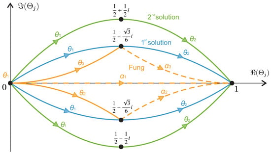
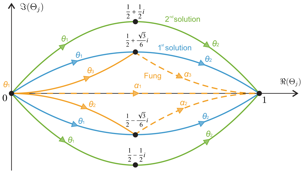
In summary, the values of the Newmark parameters and the sub-steps for the two solutions are presented in Table 1. Moreover, Figure 2 provides a schematic representation of the sub-steps with their corresponding values for both the first and second solutions, as well as those of the Fung method. In this figure, the solid lines represent the time marching with some complex sub-steps. The dashed line represent the combined solution with the sub-steps of Fung. In the sub-steps of the first and second solution, the sub-steps are executed sub-sequentially with the two sub-steps ${\theta }_1$ and ${\theta }_2$. The solutions in the first quadrant of the complex plane are distinct, however, equivalent methods of the ones in the fourth quadrant. The Fung time marching in both quadrants is the same method, although executed independently. For constructing the solution in the time step $\Delta t$, as represented in the dashed line, the solutions in each of the three time sub-steps are combined with their respective weights.

Table 1. Roots of Equations (29)–(31) (conjugates of the sub-steps and parameters are also an equivalent solution).

Solution	${\mathit{\theta }}_1$	${\mathit{\theta }}_2$	${\mathit{\gamma }}^{\mathbf{†}}$	$\mathit{\beta }$	Amplification Matrix	Load Operator Vector
$1\mathrm{st}$-sol.	${\displaystyle \frac{1}{2}}+{\displaystyle \frac{\sqrt{3}}{6}}i$	${\displaystyle \frac{1}{2}}-{\displaystyle \frac{\sqrt{3}}{6}}i$	${\displaystyle \frac{1}{2}}$	$\beta \in \mathbb{R}$	Fourth order	Fourth order
$2\mathrm{nd}$-sol.	${\displaystyle \frac{1}{2}}+{\displaystyle \frac{1}{2}}i$	${\displaystyle \frac{1}{2}}-{\displaystyle \frac{1}{2}}i$	${\displaystyle \frac{1}{2}}+{\displaystyle \frac{1}{6}}i$	${\displaystyle \frac{{\theta }_1}{6}}$	Second order *	Second order *

* If $\xi =0$ the $2\mathrm{nd}$ solution is also fourth-order accurate. ^† For different values of $\gamma$, the 1st sol. is first-order accurate, whereas the 2nd sol. remains second-order accurate.

Figure 2. Proposed complex sub-steps and Fung complex sub-steps (${\Theta }_j={\sum }_{i=1}^j{\theta }_i$).

Finally, it remains to demonstrate whether the first solution (1st) and second solution (2nd) are also fourth-order accurate for any damping ratio value. In this way, the difference between the Taylor series expansions of the analytical amplification matrix (see Appendix A) and the numerical one of the proposed approach (Equation (21)), now for an arbitrary $\xi$ for the first solution according to the sub-steps and parameters in the first line of Table 1, can be written as

$${\mathbf{A}}_{{\mathrm{N}}^2}^{1\mathrm{st}}(\Delta t)-\mathbf{A}(\Delta t)={\displaystyle \frac{i(4\beta -1)}{\sqrt{3}}}\left[\begin{array}{cc}1-4{\xi }^2& 4\xi (1-2{\xi }^2)/\omega \\ 2\xi \omega & 4{\xi }^2-1\end{array}\right]{\displaystyle \frac{{\omega }^4\Delta t^4}{4!}}+\left[\begin{array}{cc}\mathcal{O}(\Delta t^5)& \mathcal{O}(\Delta t^5)\\ \mathcal{O}(\Delta t^5)& \mathcal{O}(\Delta t^5)\end{array}\right]$$

(41)

whereas for the second solution (see the sub-steps and parameters in the second line of Table 1), one obtains

$$\begin{array}{c}\hfill {\mathbf{A}}_{{\mathrm{N}}^2}^{2\mathrm{nd}}(\Delta t)-\mathbf{A}(\Delta t)={\displaystyle \frac{1}{18}}\left[\begin{array}{cc}{d}_{11}& d_{12}\\ d_{21}& d_{22}\end{array}\right]{\displaystyle \frac{{\omega }^4\Delta t^4}{4!}}+\left[\begin{array}{cc}\mathcal{O}(\Delta t^5)& \mathcal{O}(\Delta t^5)\\ \mathcal{O}(\Delta t^5)& \mathcal{O}(\Delta t^5)\end{array}\right]\end{array}$$

(42)

where

$$\begin{array}{cc}\hfill d_{11}& =24(1+2i){\xi }^2-3i\hfill \end{array}$$

(43)

$$\begin{array}{cc}\hfill d_{12}& =\xi \left[(2+7i)-8(1+2i){\xi }^2\right]/\omega \hfill \end{array}$$

(44)

$$\begin{array}{cc}\hfill d_{21}& =(1+i)\left[12(1+2i)\xi +16(1-5i){\xi }^3\right]\omega -{\displaystyle \frac{48{\xi }^2}{\Delta t}}\hfill \end{array}$$

(45)

$$\begin{array}{cc}\hfill d_{22}& =4i\left[2(13+9i){\xi }^2-16(3+2i){\xi }^4-3\right]+{\displaystyle \frac{\xi (1-4{\xi }^2)}{\omega \Delta t}}\hfill \end{array}$$

(46)

showing that only the first solution consistently achieves fourth-order accuracy for the real response regardless of the $\xi$ and $\beta$ values, since Equation (42) regarding the second solution exhibits real terms for $\xi \ne 0$. In fact, for $\xi =0$, Equations (41) and (42) reduce to Equation (28) taking into account Equation (37) and Equation (38), respectively.

In order to demonstrate the accuracy order of the load operator vector for any value of $\xi$, we assume $t_k=0$ for simplicity, without loss of generality, and a Taylor series expansion around $t=t_k=0$ of a given force function sufficiently continuous such that one can write $f\left(t\right)=f_0^{\left(0\right)}+f_0^{\left(1\right)}t+f_0^{\left(2\right)}{t}^2/2+f_0^{\left(3\right)}{t}^3/3!+f_0^{\left(4\right)}{t}^4/4!+\mathcal{O}\left(t^5\right)$ for $t\in \left[0,\Delta t\right]$, where $f_0^{\left(i\right)}\equiv f^{\left(i\right)}\left(0\right)$. Then, the Taylor series expansions of the analytical load operator vector in Equation (16) after substituting the expressions for the analytical Green’s function and its time derivative can be written as

$$\begin{array}{c}\hfill \mathbf{L}(\Delta t,0)={\displaystyle \sum _{i=0}^3}\left[\begin{array}{c}{f}_{i-1}\\ f_i\end{array}\right]{\displaystyle \frac{\Delta t^{i+1}}{(i+1)!}}+\left[\begin{array}{c}\mathcal{O}(\Delta t^5)\\ \mathcal{O}(\Delta t^5)\end{array}\right]\end{array}$$

(47)

where $f_i=f_0^{\left(i\right)}-2\xi \omega f_0^{(i-1)}+{\omega }^2(4{\xi }^2-1)f_0^{(i-2)}-4\xi {\omega }^3(2{\xi }^2-1)f_0^{(i-3)}$, with $f_0^{\left(i\right)}=0$ for $i<0$.

After performing Taylor series expansions of the numerical load operator vector (Equation (22)) for the first solution ($1\mathrm{st}$) and second solution ($2\mathrm{nd}$), the corresponding differences from the expansions of the analytical load operator (Equation (47)) are given, respectively, by

$$\begin{array}{cc}\hfill & {\mathbf{L}}_{{\mathrm{N}}^2}^{1\mathrm{st}}(\Delta t,0)-\mathbf{L}(\Delta t,0)={\displaystyle \frac{i}{24\sqrt{3}}}\left[\begin{array}{c}(1-4\beta )f_2\\ (1-4\beta ){\omega }^2{f}_1+{\displaystyle \frac{1}{3}}{f}_0^{\left(3\right)}\end{array}\right]\Delta t^4+\left[\begin{array}{c}\mathcal{O}(\Delta t^5)\\ \mathcal{O}(\Delta t^5)\end{array}\right]\hfill \end{array}$$

(48)

$$\begin{array}{cc}\hfill & {\mathbf{L}}_{{\mathrm{N}}^2}^{2\mathrm{nd}}(\Delta t,0)-\mathbf{L}(\Delta t,0)=-{\displaystyle \frac{\xi \omega }{18}}\left[\begin{array}{c}0\\ f_1\end{array}\right]\Delta t^3+{\displaystyle \frac{\xi \omega }{36}}\left[\begin{array}{c}{f}_1\\ f_2-f_1\end{array}\right]\Delta t^4+\hfill \\ \hfill & +{\displaystyle \frac{i}{144}}\left[\begin{array}{c}{\omega }^2(16{\xi }^2-3)f_0^{\left(0\right)}-8\xi \omega f_0^{\left(1\right)}+3f_0^{\left(2\right)}\\ 2\xi {\omega }^3(16{\xi }^2-9)f_0^{\left(0\right)}+{\omega }^2(6-16{\xi }^2)f_0^{\left(1\right)}+6\xi \omega f_0^{\left(2\right)}-3f_0^{\left(3\right)})\end{array}\right]\Delta t^4+\left[\begin{array}{c}\mathcal{O}(\Delta t^5)\\ \mathcal{O}(\Delta t^5)\end{array}\right]\hfill \end{array}$$

(49)

In Equation (48) the terms of order $\Delta t^4$ are imaginary numbers. As a consequence, the load operator vector of the first solution effectively yields fourth-order accuracy (the same of its amplification matrix) for any value of $\beta \in \mathbb{R}$, including damped cases. However, the real terms of order $\Delta t^3$ and $\Delta t^4$ in Equation (49) reveal that the load operator vector for the second solution assures fourth-order accuracy only for the undamped case, otherwise the second solution becomes second-order accurate. In summary, the order of convergence of the first and second solutions is presented in Table 1.

The family of time-stepping methods with the two complex sub-steps of the first solution given in Equation (36) (adopting either ${\theta }_1=(3+i\sqrt{3})/6$ and ${\theta }_2=(3-i\sqrt{3})/6$ or ${\theta }_1=(3-i\sqrt{3})/6$ and ${\theta }_2=(3+i\sqrt{3})/6$, with both approaches being equivalent) is named hereafter as Newmark². Similar to the Newmark method, it has two free parameters, $\gamma$ and $\beta$.

For instance, by adopting $\gamma =1/2$ and $\beta =0$, the Newmark² method reproduces the CD² method [36] and when $\gamma =1/2$ and $\beta =1/4$ the method is spectrally equivalent to the fourth-order Fung method with complex sub-steps [20].

However, different from the complex sub-steps of Fung [20], the proposed method maintains fourth-order accuracy in the forced response without any further procedures. Moreover, it is worth noting that the proposed method, as opposed to the complex sub-steps of Fung, yields a solution in the complex plane (domain), where the real part represents the physical response, whereas the imaginary part reflects a numerical artifact resulting from the truncation error. The imaginary part can be discarded if not required. However, this novel feature may provide insightful information related to numerical errors in the solution. Strictly speaking, the relation between the imaginary component and the numerical errors arises because as the numerical physical response converges, the imaginary response tends to vanish (the former at the fourth-order rate and the latter at third-order rate according to Equation (41) and Equation (48), respectively). Furthermore, the imaginary component in the amplification matrix vanishes for $\beta =1/4$ in the first solution as commented previously, and it is only presented in the load operator vector (particular solution). However, the imaginary component of the load operator is still tied to the overall numerical errors. This occurs because Equation (16), considering the corresponding numerical amplification matrix and load operator vector, is applied recurrently (see also Equations (23) and (24)) and, therefore, the real errors of the amplification matrix will be multiplied by the complex errors from the previous time steps originated from the particular solution (or forced response) which possesses an imaginary component. A detailed study of the complex response in a time integration method is presented in Souza et al. [36].

3.3. Stability Analysis

The spectral radius of the amplification matrix is used to accomplish the stability analysis of the time-marching schemes of the Newmark² family. The spectral radius can be defined as $\rho \left(\mathbf{A}\right)=\underset{i}{max}\left|{\lambda }_i\left(\mathbf{A}\right)\right|$, with the eigenvalues given by

$${\lambda }_{1,2}\left(\mathbf{A}\right)=A\pm \sqrt{A^2-B}$$

(50)

for $\mathbf{A}\in {\mathbb{R}}^{2\times 2}$, where $A=\mathrm{tr}\left(\mathbf{A}\right)/2$ and $B=det\left(\mathbf{A}\right)$.

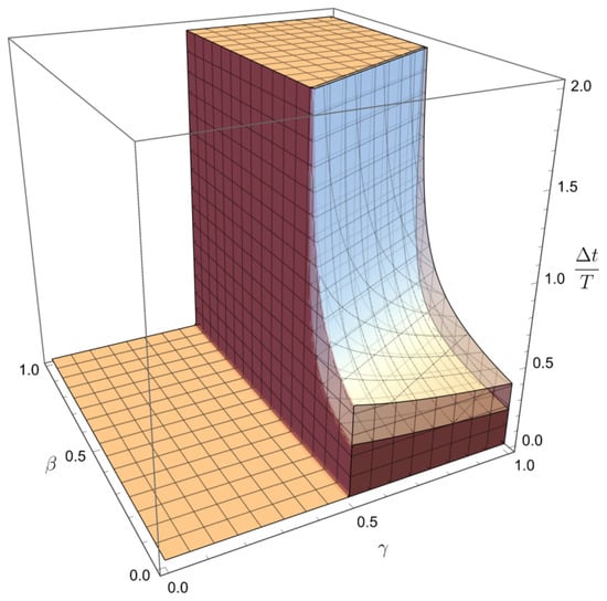
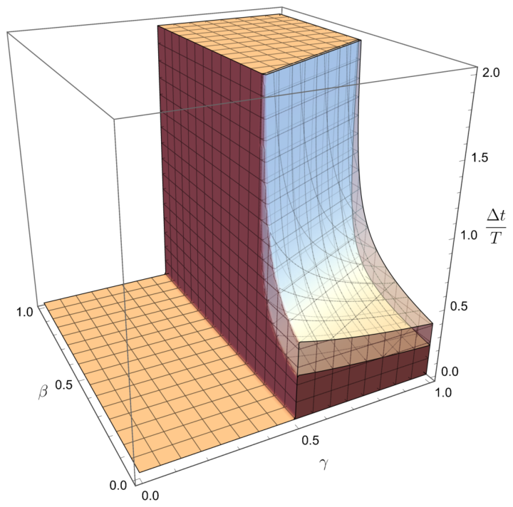
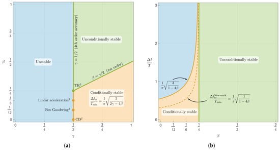
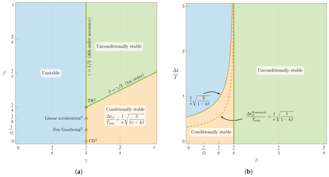
By computing the Newmark² spectral radius $\rho \left({\mathbf{A}}_{{\mathrm{N}}^2}\right)$ from Equations (21) and (50) and recalling the sub-steps of the first solution presented in Table 1, we plot the stability region (i.e, $\rho \left({\mathbf{A}}_{{\mathrm{N}}^2}\right)\le 1$) in Figure 3 as a function of $\gamma$, $\beta$, and $\Delta t/\mathrm{T}$ for $\xi =0$. The stability region of Figure 3 is very close to the classical Newmark method (opaque region in Figure 3), but with an extended conditional stability region (transparent region in Figure 3). For a deeper comprehension of the stability behavior, consider the spectral stability as a function of the Newmark parameters $\gamma$ and $\beta$ presented in Figure 4a and the spectral stability for $\gamma =1/2$ in Figure 4b (slices in Figure 3 in $\Delta t/T\to \infty$ and $\gamma =1/2$, respectively). These figures show that the proposed method (as the classical Newmark method) is unstable for $\gamma <1/2$ (blue region in Figure 4a, where $\rho \left({\mathbf{A}}_{{\mathrm{N}}^2}\right)>1\forall \Delta t/T$), unconditionally stable for $\gamma \ge 1/2$ and $\beta \ge \gamma /2$ (green regions in Figure 4, where $\rho \left({\mathbf{A}}_{{\mathrm{N}}^2}\right)\le 1\forall \Delta t/T$), and conditionally stable for $\gamma \ge 1/2$ and $\beta <\gamma /2$ (orange regions in Figure 4, where $\rho \left({\mathbf{A}}_{{\mathrm{N}}^2}\right)\le 1\forall \Delta t\le \Delta t_{\mathrm{cr}}$). However, the critical time step for the conditionally stable region of the Newmark² with $\xi =0$ is given by

$${\displaystyle \frac{\Delta t_{\mathrm{cr}}}{T_{\min }}}={\displaystyle \frac{1}{\pi }}\sqrt{{\displaystyle \frac{3}{2\gamma -4\beta }}}$$

(51)

which is higher than the critical time step of the classical Newmark method by a factor of $\sqrt{3}$ (see Figure 4b).

Figure 3. Improved Newmark² stability region over the classical Newmark method for $\xi =0$.

Figure 4. Spectral stability region of the Newmark² method for $\xi =0$ as a function of (a) $\gamma$ and $\beta$; and (b) $\beta$ and $\Delta t/T$ for $\gamma =1/2$ (fourth-order accuracy).

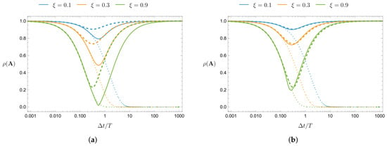
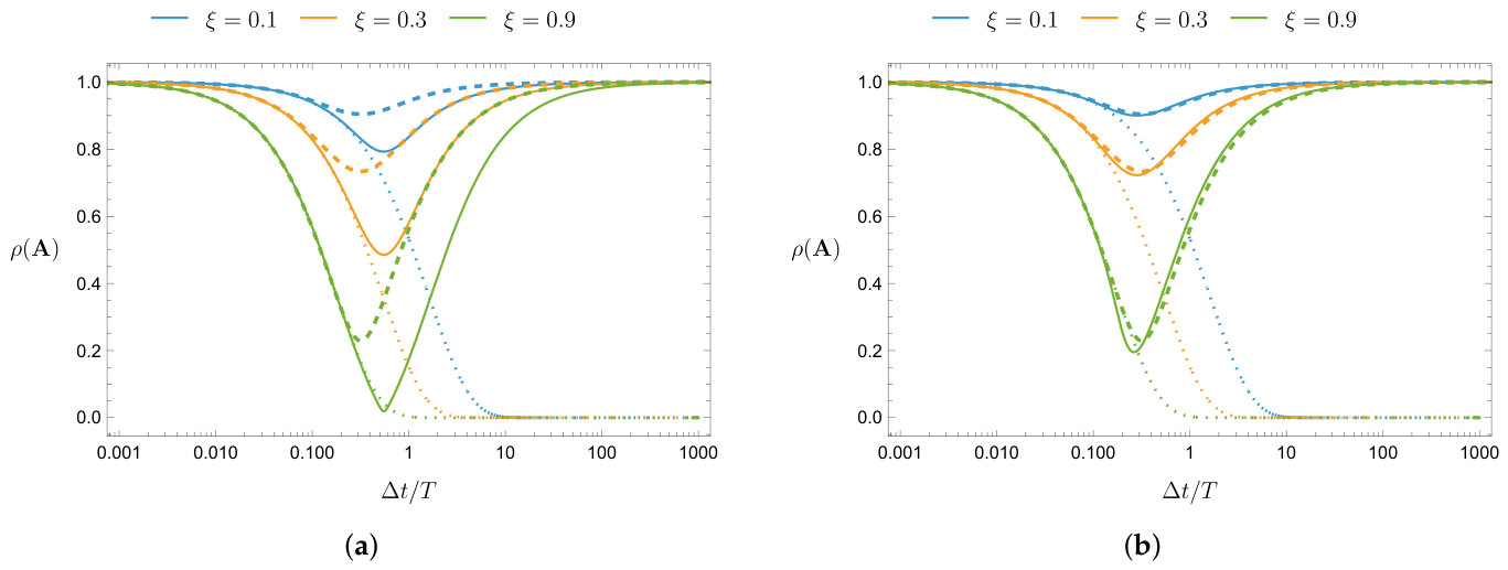
As a consequence, the Central Difference method ($\gamma =1/2$ and $\beta =0$), Fox and Goodwing method ($\gamma =1/2$ and $\beta =1/12$) and linear acceleration method ($\gamma =1/2$ and $\beta =1/6$), represented in the orange points in Figure 4a [2,3], as any other method within the Newmark family with $\gamma =1/2$, become fourth-order accurate with a higher stability limit. This increase in the stability is also depicted in Figure 4b, where the orange dashed line represents the critical time step of the Newmark family and the continuous one the critical time step of the Newmark² for the parameters $\gamma =1/2$ and $\beta <1/4$. Observe also the increase in the stability region (i.e., in the critical time step value) for $\gamma \in (1/2,1)$ and $\beta <\gamma /2$ in the transparent and solid regions of Figure 3, illustrating that each conditionally stable scheme within the Newmark family exhibits an increase in the stability limit by a factor of $\sqrt{3}$. Finally, it is readily verified that the unconditional stability for physical damping cases is assured as well. For instance, Figure 5 shows a comparison of spectral radii for some values of $\xi$ considering $\gamma =1/2$ and $\beta =1/4$, where the curves associated with the Newmark² method exhibit greater proximity to the analytical ones than those obtained using the Newmark and Tarnow and Simo methods. A summary of the improvements for these members of the Newmark² method over the original Newmark method is presented in Table 2 and Table 3.

Figure 5. Comparison of spectral radii as a function of the damping ratio $\xi$ considering $\gamma =1/2$ and $\beta =1/4$ among the analytical (⋯), the Newmark method (- - -), and (a) the Newmark² method (–); and (b) the Tarnow and Simo method (–).

Table 2. Properties of well-known members of the Newmark family (including non-null load operator vector and physical damping ratio).

Method	Type	$\mathit{\gamma }$	$\mathit{\beta }$	Stability Condition $\mathbf{(}\mathbf{\Delta }{\mathit{t}}_{\mathbf{cr}}/{\mathit{T}}_{\mathbf{min}}\mathbf{)}$	Order of Accuracy
Trapezoidal Rule (TR)	Implicit	$1/2$	$1/4$	Unconditional	2
Linear Acceleration	Implicit	$1/2$	$1/6$	$\sqrt{3}/\pi$	2
Fox–Goodwin	Implicit	$1/2$	$1/12$	$\sqrt{3/2}/\pi$	2
Central Difference (CD)	Explicit	$1/2$	0	$1/\pi$	2

Table 3. Properties of proposed members of the Newmark² family (including non-null load operator vector and physical damping ratio).

Method	Type	$\mathit{\gamma }$	$\mathit{\beta }$	Stability Condition $\mathbf{(}\mathbf{\Delta }{\mathit{t}}_{\mathbf{cr}}/{\mathit{T}}_{\mathbf{min}}\mathbf{)}$	Order of Accuracy
Trapezoidal Rule2 (TR2)	Implicit	$1/2$	$1/4$	Unconditional	4
Linear Acceleration2	Implicit	$1/2$	$1/6$	$3/\pi$	4
Fox–Goodwin2	Implicit	$1/2$	$1/12$	$3/\left(\sqrt{2}\pi \right)$	4
Central Difference2 (CD2)	Explicit	$1/2$	0	$\sqrt{3}/\pi$	4

Similar to the Newmark method, in the Newmark² method, it is only possible to introduce numerical damping for $\gamma >1/2$; however, the method becomes first-order accurate only (see Section 3.2). Nevertheless, in many practical structural dynamic applications, the numerical damping is unnecessary, meaning that a non-dissipative scheme is preferred. In these cases, the classical Newmark method with $\gamma =1/2$ is very well suited and, as a consequence, the Newmark² method as well because it inherits some of the classical Newmark properties.

For the proposed Newmark² family of methods, the parameters can be selected with an analogous perspective of the classical Newmark family, i.e., (i) $\gamma =1/2$ is preferred to maintain the fourth-order accuracy in the Newmark² method (or second-order in the Newmark method) and (ii) the family of methods with $\beta <1/4$ are conditionally stable. However, for $\beta \ge 1/4$, the numerical errors increase with $\beta$. For this reason, in implicit approaches, we recommend adopting $\beta =1/4$ and $\gamma =1/2$, i.e., the well-known trapezoidal rule (represented in the green point TR² in Figure 4a and the green line in Figure 4b), for achieving simultaneously unconditional stability, fourth-order accuracy, and very low numerical errors. In problems where explicit approaches are well suited, we recommend the parameter values $\beta =0$ and $\gamma =1/2$ to reproduce the recent explicit method proposed in Souza et al. [36] (represented in the orange point CD² in Figure 4a).

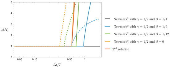
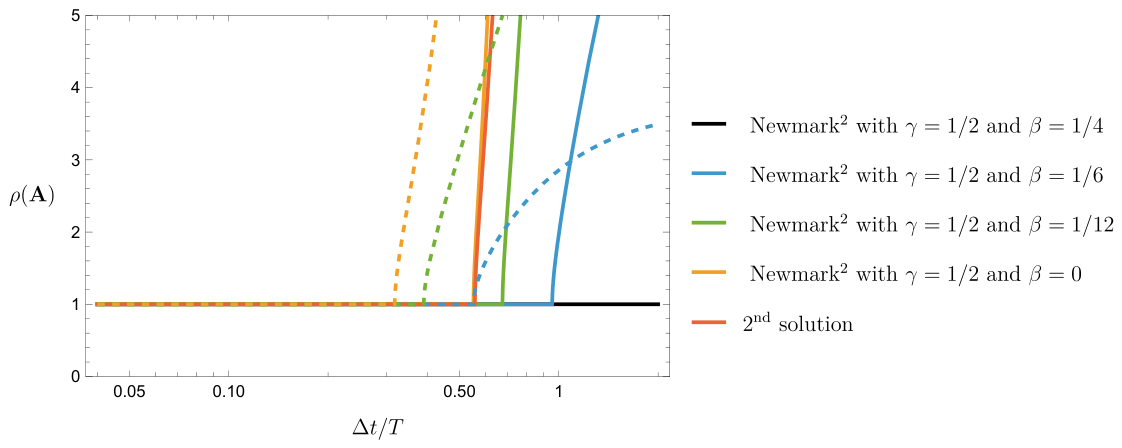
Until now, we have only discussed the stability concerning the sub-steps of the first solution (Table 1). In order to study the stability of the second solution, in Figure 6, we compare the spectral radius $\rho \left({\mathbf{A}}_{{\mathrm{N}}^{\mathbf{2}}}\right)$ for the first and second solutions (Table 1). Figure 6 shows that the first solution increases the stability of the classical Newmark according to Equation (51), whereas the second solution has a critical time step of $\Delta t_{\mathrm{cr}}/T_{\min }\approx 0.557$, which is close to the critical time step of the first solution with $\beta =0$. However, although the second solution is also conditionally stable, the method cannot be implemented in an explicit manner since $\beta \ne 0$. Finally, it is important to stress that this work focuses only on unconditionally stable fourth-order accurate methods for solving the structural dynamic problems; therefore, further investigation of the second solution will not be presented hereafter.

Figure 6. Spectral radii of the Newmark method with two sub-steps (—) compared to the classical Newmark method (- - -) for $\xi =0$.

3.4. Measurement Errors

Finally, to measure and compare the errors, the relative period elongation and numerical damping are calculated. The numerical damping ratio $\overline{\xi }$ and numerical frequency $\overline{\omega }$ are related to the complex eigenvalues of the amplification matrix according to the following equation [3]:

$$\begin{array}{c}\hfill {\lambda }_{1,2}\left(\mathbf{A}\right)=\exp \left(\overline{\omega }\Delta t(-\overline{\xi }\pm i\sqrt{1-{\xi }^2})\right)\end{array}$$

(52)

From Equations (52) and (50) we obtain the following:

$$\begin{array}{cc}\hfill \overline{\omega }& ={\displaystyle \frac{\overline{\Omega }}{\Delta t}}\hfill \end{array}$$

(53)

$$\begin{array}{cc}\hfill \overline{\xi }& =-{\displaystyle \frac{ln\rho \left(\mathbf{A}\right)}{\overline{\Omega }}}\hfill \end{array}$$

(54)

where $\overline{\Omega }=2\pi \Delta t/\overline{T}=arctan\left(\sqrt{(B/A^2)-1}\right)/\sqrt{1-{\xi }^2}$.

The relative period elongation (or relative period error) can be calculated as [3]

$$\begin{array}{c}\hfill PE={\displaystyle \frac{\overline{T}-T}{T}}={\displaystyle \frac{\Omega }{\overline{\Omega }}}-1\end{array}$$

(55)

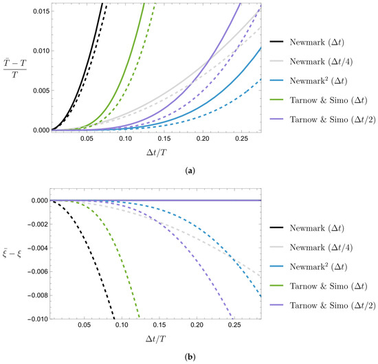
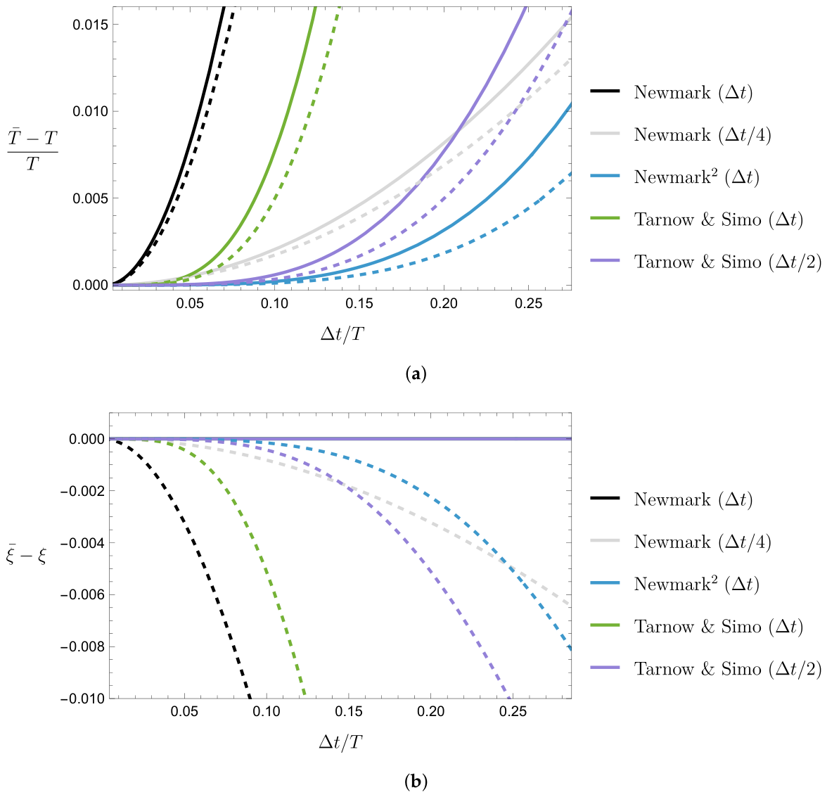
The numerical damping ratio and relative period elongation are calculated, respectively, with Equations (54) and (55) for $\xi =0$ and $\xi =0.2$ considering the Tarnow and Simo, Newmark² and Newmark methods with the trapezoidal rule (the Fung sub-steps shares the same amplification matrix of the Newmark² method for the trapezoidal rule). The results are presented in Figure 7, where we can observe that errors of the fourth-order Newmark² method are smaller than those of the second-order Newmark method or the fourth-order Tarnow and Simo method. Even when the Newmark method uses a time step four times smaller, or the Tarnow and Simo method uses a time step two times smaller, they still exhibit more numerical errors than the proposed method. The use of complex sub-steps leads to reduced numerical dissipation and dispersion measures that cannot be achieved with real sub-steps. In addition, the proposed method, like the classic Newmark method, have no numerical (algorithmic) damping for $\xi =0$ and $\gamma =1/2$.

Figure 7. Numerical dissipation and dispersion errors for $\xi =0$ (—) and $\xi =0.2$ (- - -) considering the trapezoidal rule: (a) relative period elongation and (b) numerical damping ratio.

3.5. Computer Implementation

The implementation of the new family of time integration methods that achieves fourth-order accuracy based on the first solution developed in the previous subsections with $\gamma =1/2$ and complex sub-steps according to Equation (36) in the Newmark’s family is summarized in Algorithm 1. As can be observed, the proposed schemes are straightforwardly implemented into existing structural dynamics codes based on the classical Newmark method by just calling the Newmark subroutine twice and sequentially to carry out the computations required by the two complex sub-steps whitin each time step $\Delta t$. It should be noted that the computed displacement, velocity and acceleration solution vectors consist of complex numbers, i.e., ${\mathbf{U}}^{k+1},{\dot{\mathbf{U}}}^{k+1},{\ddot{\mathbf{U}}}^{k+1}\in {\mathbb{C}}^N$, implying that the code must be adapted to handle complex variables. Strictly speaking, the use of complex arithmetic operations inevitably increases the overall computational cost. Nevertheless, for the small- to medium-scale structural dynamic problems modeled, for instance, as truss, frame, and beam, this is often not a concern in view of the high accuracy provided by the proposed Newmark² method. On the other hand, for large-scale problems, particularly those involving solid finite elements in 3D continua, the cost may become an issue on some applications, and certain aspects of the algorithm should be considered.

Algorithm 1 Time integration with the implicit Newmark2 method

1: Calculate the initial acceleration vector ${\ddot{\mathbf{U}}}^0={\mathbf{M}}^{-1}\left[{\mathbf{F}}^0-\mathbf{C}{\dot{\mathbf{U}}}^0-\mathbf{K}{\mathbf{U}}^0\right]$.   2: Select the time-step size $\Delta t$ and the number of time steps n.   3: Select the complex sub-steps ${\theta }_1$ and ${\theta }_2$ of the $1\mathrm{st}$ solution (Table 1) and the Newmark parameters $\gamma$ and $\beta$ (select $\gamma =1/2$ for $4\mathrm{th}$ order accuracy and $\beta =1/4$ for unconditional stability with lower numerical errors).   4: Calculate the complex-valued integration constants $a_{0,j}={\theta }_j\Delta t$, $a_{1,j}=(1-2\beta )a_{0,j}^2/2$, $a_{2,j}=(1-\gamma )a_{0,j}$, $a_{3,j}=\beta a_{0,j}^2$ and $a_{4,j}=\gamma a_{0,j}$, with $j=1,2$.   5: Calculate the effective stiffness matrix ${\mathbf{K}}_{\mathrm{eff},1}=\mathbf{M}+a_{4,1}\mathbf{C}+a_{3,1}\mathbf{K}$ and triangularize it (for the second sub-step one readily obtains ${\mathbf{K}}_{\mathrm{eff},2}={\overline{\mathbf{K}}}_{\mathrm{eff},1}$).   6: for $k=0$, …, $n-1$ do   (a) Newmark with the first sub-step:                    ▹ First sub-step $\begin{array}{l}{\mathbf{U}}_{\mathrm{p}}^{k+{\theta }_1}={\mathbf{U}}^k+a_{0,1}{\dot{\mathbf{U}}}^k+a_{1,1}{\ddot{\mathbf{U}}}^k\\ {\dot{\mathbf{U}}}_{\mathrm{p}}^{k+{\theta }_1}={\dot{\mathbf{U}}}^k+a_{2,1}{\ddot{\mathbf{U}}}^k\end{array}\}\mathrm{Predictors}$         ▹ Compute predictors at $(k+{\theta }_1)\Delta t$ ${\mathbf{K}}_{\mathrm{eff},1}{\ddot{\mathbf{U}}}^{k+{\theta }_1}={\mathbf{F}}^{k+{\theta }_1}-\mathbf{C}{\dot{\mathbf{U}}}_{\mathrm{p}}^{k+{\theta }_1}-\mathbf{K}{\mathbf{U}}_{\mathrm{p}}^{k+{\theta }_1}$           ▹ Solve for accelerations at $(k+{\theta }_1)\Delta t$ $\begin{array}{l}{\mathbf{U}}^{k+{\theta }_1}={\mathbf{U}}_{\mathrm{p}}^{k+{\theta }_1}+a_{3,1}{\ddot{\mathbf{U}}}^{k+{\theta }_1}\\ {\dot{\mathbf{U}}}^{k+{\theta }_1}={\dot{\mathbf{U}}}_{\mathrm{p}}^{k+{\theta }_1}+a_{4,1}{\ddot{\mathbf{U}}}^{k+{\theta }_1}\end{array}\}\mathrm{Correctors}$  ▹ Compute displacements and velocities at $(k+{\theta }_1)\Delta t$   (b) Newmark with the second sub-step:                  ▹ Second sub-step $\begin{array}{l}{\mathbf{U}}_{\mathrm{p}}^{k+1}={\mathbf{U}}^{k+{\theta }_1}+a_{0,2}{\dot{\mathbf{U}}}^{k+{\theta }_1}+a_{1,2}{\ddot{\mathbf{U}}}^{k+{\theta }_1}\\ {\dot{\mathbf{U}}}_{\mathrm{p}}^{k+1}={\dot{\mathbf{U}}}^{k+{\theta }_1}+a_{2,2}{\ddot{\mathbf{U}}}^{k+{\theta }_1}\end{array}\}\mathrm{Predictors}$         ▹ Compute predictors at $(k+1)\Delta t$ ${\overline{\mathbf{K}}}_{\mathrm{eff},1}{\ddot{\mathbf{U}}}^{k+1}={\mathbf{F}}^{k+1}-\mathbf{C}{\dot{\mathbf{U}}}_{\mathrm{p}}^{k+1}-\mathbf{K}{\mathbf{U}}_{\mathrm{p}}^{k+1}$              ▹ Solve for accelerations at $(k+1)\Delta t$ $\begin{array}{l}\hfill {\mathbf{U}}^{k+1}={\mathbf{U}}_{\mathrm{p}}^{k+1}+a_{3,2}{\ddot{\mathbf{U}}}^{k+1}\\ {\dot{\mathbf{U}}}^{k+1}={\dot{\mathbf{U}}}_{\mathrm{p}}^{k+1}+a_{4,2}{\ddot{\mathbf{U}}}^{k+1}\end{array}\}\mathrm{Correctors}$    ▹ Compute displacements and velocities at $(k+1)\Delta t$  Print the solutions $\Re ({\mathbf{U}}^{k+1},{\dot{\mathbf{U}}}^{k+1},{\ddot{\mathbf{U}}}^{k+1})$ (and $\Im ({\mathbf{U}}^{k+1},{\dot{\mathbf{U}}}^{k+1},{\ddot{\mathbf{U}}}^{k+1})$ if required).   7: end for

An important aspect of the method is that the sub-steps are complex conjugate numbers, and therefore the effective stiffness matrices are also complex conjugates (i.e., ${\mathbf{K}}_{\mathrm{eff},2}={\overline{\mathbf{K}}}_{\mathrm{eff},1}$). This feature reduces the overall computational cost by eliminating the need to triangularize an additional effective stiffness matrix, since the conjugate of the first effective stiffness matrix factorization can be reused for the second sub-step. Although not common in time-domain analyses, the system of equations with complex numbers frequently appears in structural dynamics, particularly in the frequency domain [40], as well as in other fields like electromagnetics [41,42]. In addition, recent solvers often supports complex-valued systems [42]. Thus, significant advancements in solving this complex-valued system efficiently have been accomplished using both direct and iterative solvers [42]. The effective stiffness complex-valued matrix ${\mathbf{K}}_{\mathrm{eff},1}\in {\mathbb{C}}^{N\times N}$ of Algorithm 1 can, in principal, be converted into an equivalent real-valued matrix by doubling its dimensions, i.e., ${\tilde{\mathbf{K}}}_{\mathrm{eff},1}\in {\mathbb{R}}^{2N\times 2N}$ (the reader is refereed to Higham [43] and Marioni et al. [44] for a more in-depth discussion of such a conversion). Hence, it follows that computing the solution of a linear system with N complex equations is equivalent of solving a real system with $2N$ equations. However, as pointed out by Higham [43], who focused on direct solvers, true complex formulation outperforms the equivalent real approaches for solving complex-valued linear systems. In fact, nowadays, many robust solvers such as PARDISO (PARallel DIrect SOlver) and MUMPS (MUltifrontal Massively Parallel Sparse direct Solver) can handle the solution of sparse complex linear systems of equations directly in an efficient manner using modern parallel architectures [42].

It is noteworthy, that in the complex Fung method, the solutions on conjugate sub-steps are computed independently (Figure 2), allowing the response corresponding to one sub-step to be obtained directly from the other without recomputing the system, thus reducing the computational effort. However, for large-scale problems, the computational cost is heavily dominated by the factorization of the effective stiffness matrix. Although the computational effort to compute the factorization of complex-valued matrices requires about three times the computational effort to compute the factorization of real matrices on modern computer architectures [45], the proposed method mitigates this overhead through a key algorithm to perform only a single matrix factorization. In this sense, an analytical comparison of the computational effort can be established based on floating-point operations (FLOPs) for solving large-scale problems. If the FEM matrices are assumed to be $N_b$-banded and recalling that N is the number of DOFs, a Cholesky decomposition in methods with a single symmetric real-valued stiffness matrix, like the Newmark method, requires approximately $N{N}_b^2$ FLOPs. In contrast, methods that utilizing a single complex-valued stiffness matrix require about $3N{N}_b^2$ FLOPs for the factorization. Finally, unlike the Fung method or any other unconditionally stable time integration method, an additional important aspect stems from the fact that the imaginary component of the computed solution vectors, i.e., $\Im ({\mathbf{U}}^{k+1},{\dot{\mathbf{U}}}^{k+1},{\ddot{\mathbf{U}}}^{k+1})$ can be employed as an indicator of the errors in the solution as analyzed later in the numerical examples.

4. Numerical Experiments

In what follows, to illustrate the performance of the proposed method and validate the theoretical findings, we solve and analyze two numerical examples using the Newmark, Newmark², Tarnow and Simo, and Fung methods as described in Section 3, all employing the trapezoidal rule (i.e., $\gamma =1/2$ and $\beta =1/4$). In these problems, we do not modify the external load vector to adjust it to a specific time integration method, unlike the procedure discussed in Fung [20]; instead, the load vector is directly applied as usual. The first example considers a simple frame structure with rigid beams and inextensible columns, introduced to demonstrate the order of accuracy in the presence of external load and physical damping. The second example deals with a 3D elastodynamic model discretized by the finite element method. Only the real part of the computed solutions is considered in the graphics, unless explicitly stated otherwise, thereby always avoiding the use of the notation $\Re \left(·\right)$ when plotting solutions. Moreover, the imaginary component in the examples arises only due the load operator, since we use $\beta =1/4$, which leads to a real-valued homogeneous solution and a complex-valued particular solution according to Section 3.2.

4.1. Shear Building

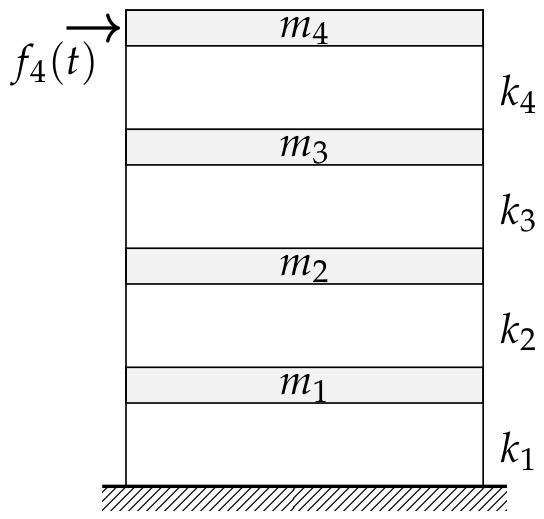
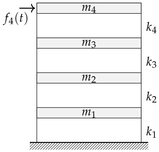
In this first example, in order to present the performance of the proposed method, in a general case, including external forces and physical damping, as theoretically demonstrated in Section 3.2, we analyze a four-floor shear building, as illustrated in Figure 8, described by the following initial-value problem with null initial conditions:

$$\begin{array}{c}\hfill \left[\begin{array}{cccc}{m}_1& 0& 0& 0\\ 0& m_2& 0& 0\\ 0& 0& m_3& 0\\ 0& 0& 0& m_4\end{array}\right]\left[\begin{array}{c}{\ddot{U}}_1\left(t\right)\\ {\ddot{U}}_2\left(t\right)\\ {\ddot{U}}_3\left(t\right)\\ {\ddot{U}}_4\left(t\right)\end{array}\right]+\left[\begin{array}{cccc}{c}_{11}& c_{12}& 0& 0\\ c_{21}& c_{22}& c_{23}& 0\\ 0& c_{32}& c_{33}& c_{34}\\ 0& 0& c_{43}& c_{44}\end{array}\right]\left[\begin{array}{c}{\dot{U}}_1\left(t\right)\\ {\dot{U}}_2\left(t\right)\\ {\dot{U}}_3\left(t\right)\\ {\dot{U}}_4\left(t\right)\end{array}\right]+\\ \hfill +\left[\begin{array}{cccc}{k}_1+k_2& -k_1& 0& 0\\ -k_1& k_2+k_3& -k_3& 0\\ 0& -k_3& k_3+k_4& -k_4\\ 0& 0& -k_4& k_4\end{array}\right]\left[\begin{array}{c}{U}_1\left(t\right)\\ U_2\left(t\right)\\ U_3\left(t\right)\\ U_4\left(t\right)\end{array}\right]=\left[\begin{array}{c}0\\ 0\\ 0\\ f_4\left(t\right)\end{array}\right]\end{array}$$

(56)

with $m_1=m_2=m_3=m_4=1$, $k_1=40$, $k_2=35$, $k_3=30$, $k_4=25$, and $f_4\left(t\right)=sin\left(t\right)$, whereas entries $c_{ij}$ of the proportional damping matrix correspond to the Rayleigh coefficients of $0.2$ and $0.002$ for the mass and stiffness matrices, respectively (damping ratio of approximately $2\%$ and $5\%$ into the higher and lower modes of the system, respectively).

Figure 8. Shear building model with four stories.

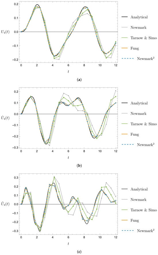
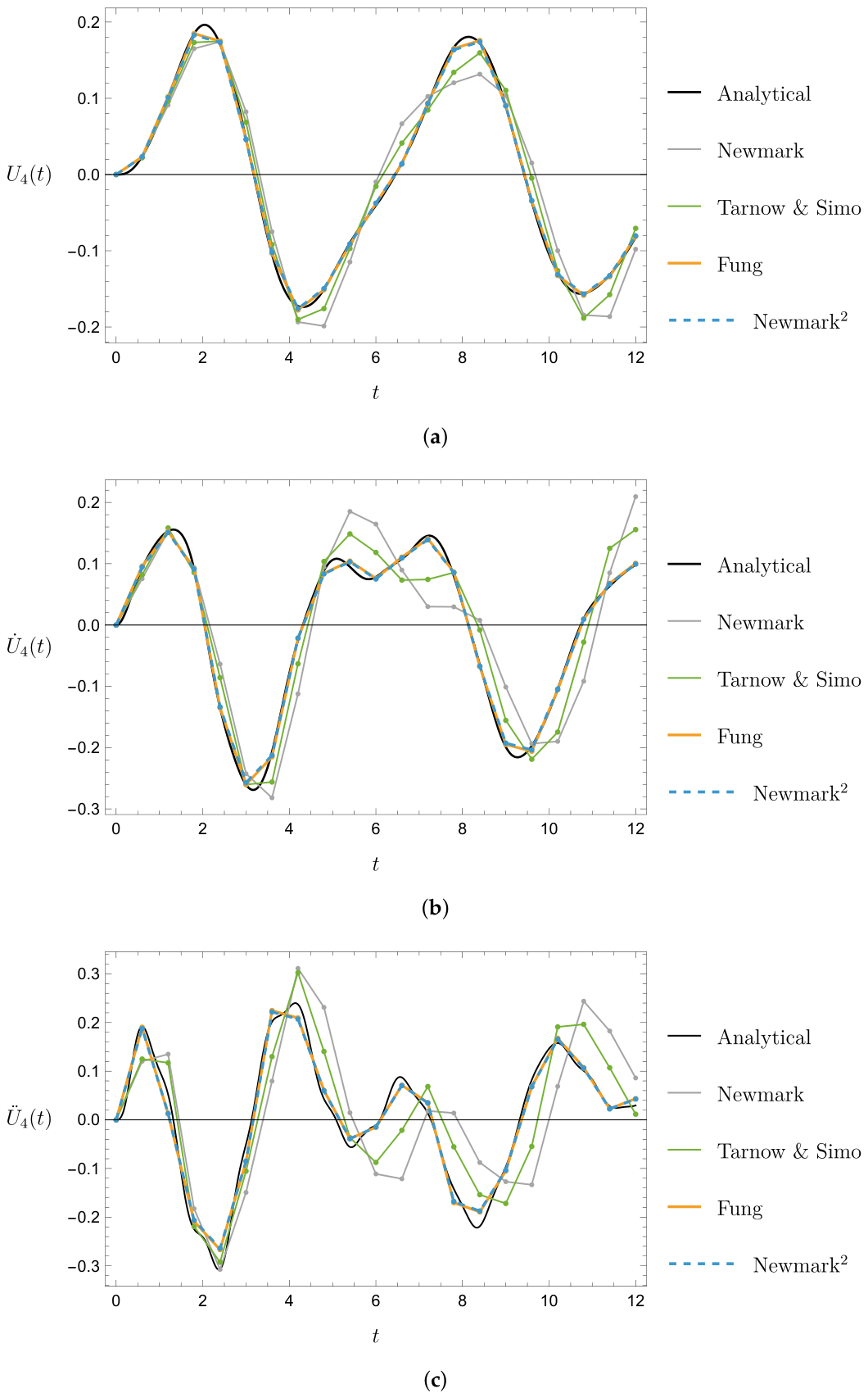
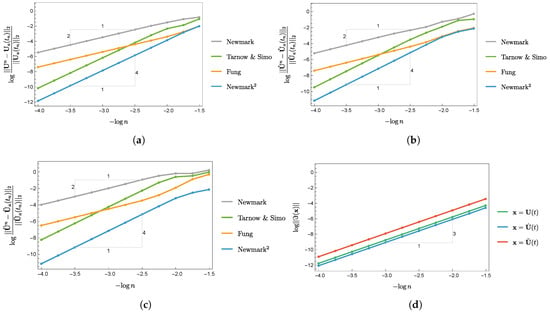
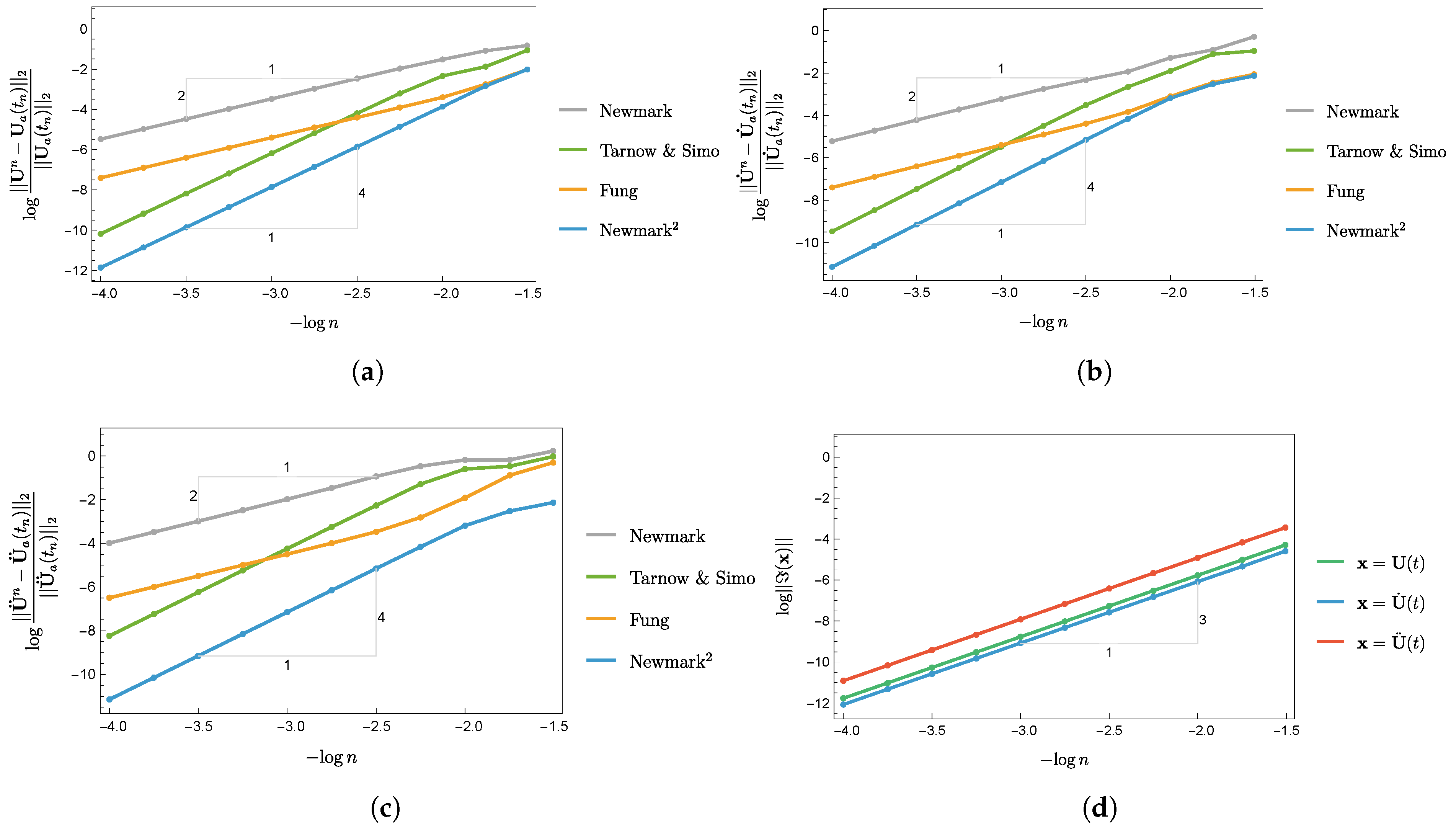
We compute both the displacement, velocity, and acceleration vectors considering various time-step sizes to analyze the corresponding convergence rates with the Euclidean norm at the time instant $t_n=12$. The analytical solution vector ${\mathbf{U}}_a\left(t\right)$ is obtained by decoupling the system through modal analysis and solving each SDOF equation analytically according to Equation (16). The maximal and minimal periods of the system are given by $T_{\min }\approx 0.589$ and $T_{\max }\approx 3.059$. Figure 9 presents the solution of the displacement, velocity, and acceleration and Figure 10 presents the convergence rate, including the imaginary component. The results are in perfect agreement with the theoretical predictions of Section 3. Figure 9 shows that the second-order Newmark and the fourth-order Tarnow and Simo methods fail to produce accurate results for $\Delta t=0.6$. Only the fourth-order Newmark² and Fung methods yield accurate results for this time-step size and time range of analysis. However, in this example, the Fung method becomes second-oder accurate for the displacement, velocity and acceleration results, while the other methods preserve the same order of accuracy of their amplification matrices as can be observed in Figure 10a–c. Furthermore, the proposed Newmark² method provides an imaginary component in the solution that is related to its numerical errors. This is a novel numerical property, studied recently by Souza et al. [36]. The relation arises because, as the numerical response converges to the analytical one, the imaginary component approaches to zero with a global convergence rate of 3 (see Figure 10d), which is in agreement with Equation (48), which exhibits local terms of order $\Delta t^4$.

Figure 9. Time-history results of the fourth floor: (a) displacement, (b) velocity, and (c) acceleration.

Figure 10. Convergence rates of the (a) displacement, (b) velocity, (c) acceleration, and (d) their respective imaginary components. The numbers inside the small gray triangles (1, 2, and 4) are slope indicator that directly represents the order of accuracy of the numerical method.

4.2. Three-Dimensional Structure

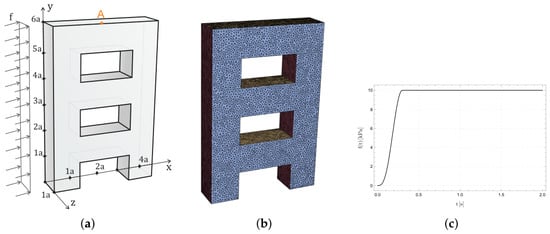
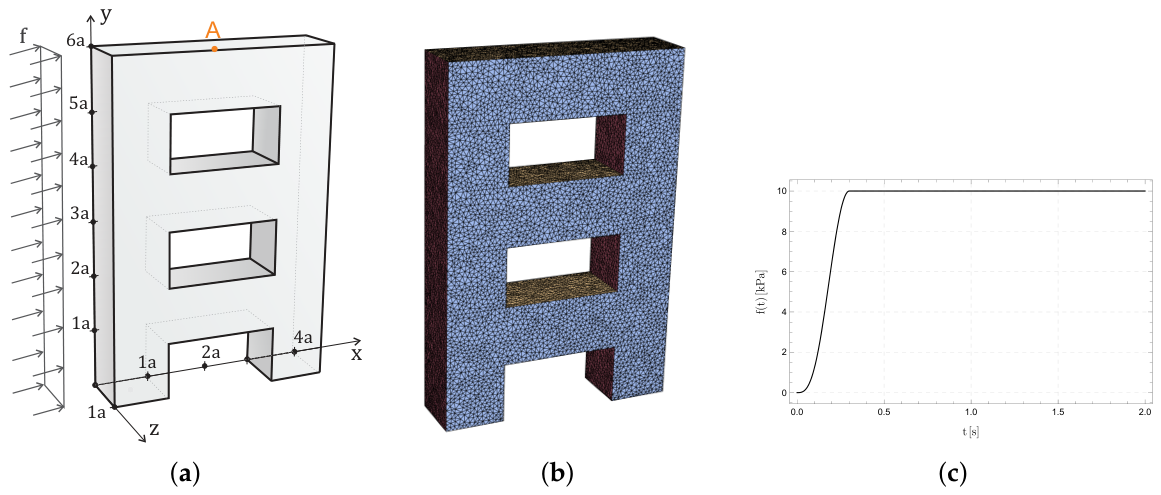
Consider a perforated solid with the base fixed, null initial conditions, and subjected to a lateral dynamic loading as illustrated in Figure 11 [31,46]. The dimensions are indicated in the figure with $a=2$ m. The material properties are Young’s modulus $E=2\times {10}^8$ Pa, mass density $\rho =2\times {10}^4$ kg/m³, and Poisson’s ratio $\nu =0.2$. The variation of the load with respect to time is given by

$$\begin{array}{c}\hfill f\left(t\right)=\left\{\begin{array}{cc}P{sin}^3\left({\displaystyle \frac{\pi t}{2t_0}}\right),\hfill & t\in [0,t_0]\hfill \\ P,\hfill & t>t_0\hfill \end{array}\right.\end{array}$$

(57)

with $P={10}^4$ Pa and $t_0=0.3$ s.

Figure 11. Three-dimensional structure model: (a) boundary conditions and geometry definitions, (b) 3D finite element mesh, and (c) dynamic loading function.

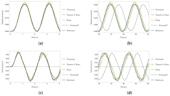
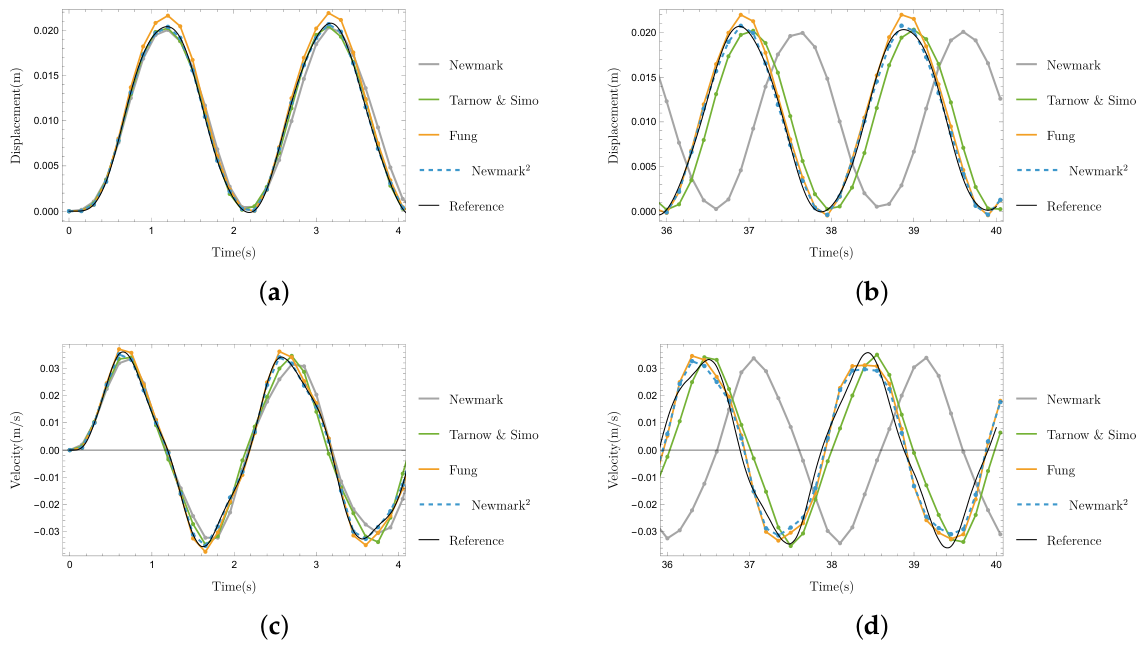
The domain is discretized into 274,050 linear tetrahedron elements, and the solution is computed up to $t_f=40$ s. Figure 12 presents the results of the displacement and velocity at point A$(2a,6a,a)$ in the $\mathrm{x}$ direction for the first and last $4$ s of the analysis. The reference solution is computed with the Newmark method with a small time step of size $\Delta t=1.5\times {10}^{-3}$ s. Since we are using non-dissipative implicit time integration methods, large time-step sizes are allowed. In this case, we choose to compare the methods with a large time-step size of $\Delta t=0.15$ s. The proposed Newmark² method achieves the most accurate results. The Fung complex method, although spectrally equivalent to the proposed Newmark² method, cannot achieve accurate results, even in the beginning of the analysis due to the error originated from the load operator (particular solution). Furthermore, for a long time duration analysis, the classical Newmark method and even the fourth-order method of Tarnow and Simo suffer from high period elongation.

Figure 12. Time-history results at point A$(2a,6a,a)$ of (a) displacement at $t\in [0,4]$ s and (b) $t\in [36,40]$ s; (c) velocity at $t\in [0,4]$ s and (d) $t\in [36,40]$ s.

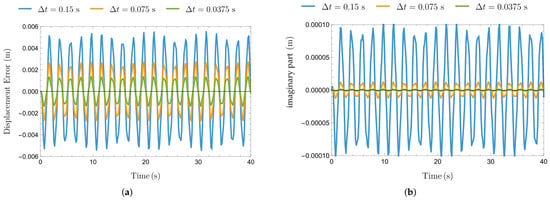
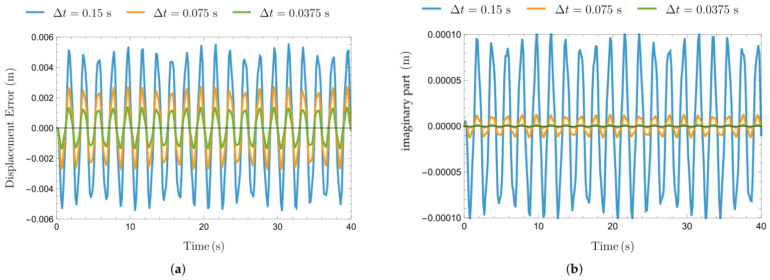
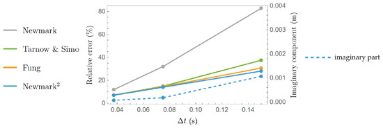
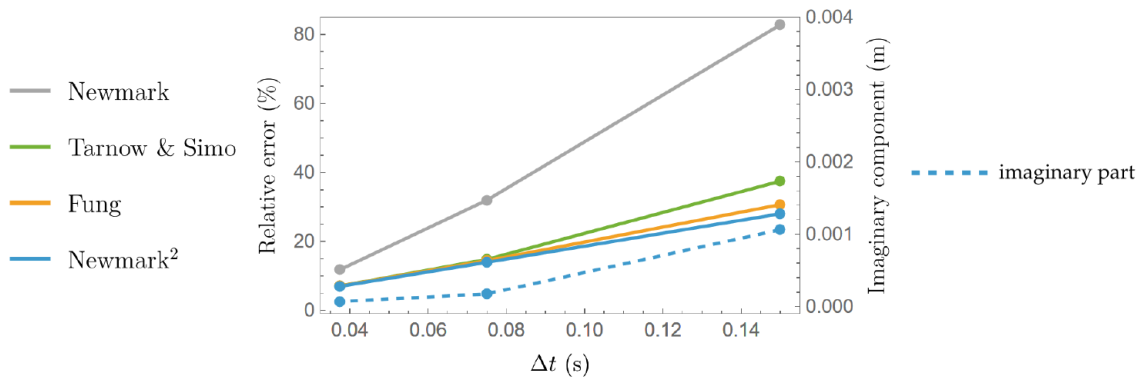
To further investigate the numerical features of the Newmark² method, the error and the imaginary part of the displacement at nodal point A$(2a,6a,a)$ are compared and analyzed. To this end, the problem is resolved considering two additional smaller time steps of sizes $\Delta t=0.075$ s and $\Delta t=0.0375$ s. Figure 13 shows the evolution of the error (defined by the difference between the reference and the Newmark² solutions) and the imaginary part of the displacement along with the time. One can observe a strong correspondence of the imaginary part to the error in the sense that both decrease with a reduction in time-step size. It also shows that the imaginary part captures quite well the same behavior of the error curve. In fact, although they are in phase, amplitudes do not coincide as expected since the imaginary part is only related to the remainder in the Taylor series expansions of the particular solution (see Equation (48)). Such behavior has already been observed in a series of numerical examples presented and studied by Souza et al. [36]. Furthermore, to better visualize the reduction in both the error and the imaginary part as $\Delta t$ decreases in different scales, Figure 14 depicts a comparative analysis of the relative percentage error at the end of the simulation (i.e., $t_f=40$ s), also considering the other methods. In this way, the imaginary component may act as a tool that indicates whether accurate results are being achieved.

Figure 13. Time-history results at point A$(2a,6a,a)$ of (a) numerical errors of the displacement and (b) imaginary component for $t\in [0,40]$ s.

Figure 14. Percentage relative error and imaginary part of the displacement at point A$(2a,6a,a)$ and $t=40$ s with $\Delta t=0.15$ s, $\Delta t=0.075$ s, and $\Delta t=0.0375$ s.

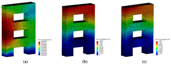
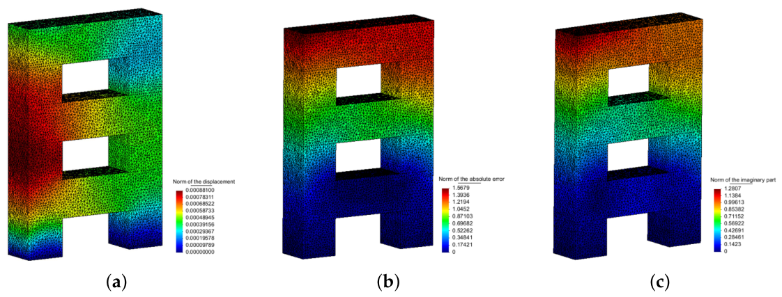
The key information in Figure 13 lies in the distribution of the error in the time domain provided by the imaginary part as previously discussed. However, the relationship between the magnitude of the imaginary part and the error, in addition to not being coincident, varies for each degree of freedom. As a result, the spatial distribution of the error does not always mirror that of the imaginary part due to the different scales encountered in the imaginary component over the degrees of freedom. Nonetheless, at certain time instants, a significant correspondence can still be observed; for example, the displacement errors at $t=4$ s shown in Figure 15.

Figure 15. Contours of the norm of the nodal components for (a) displacement, (b) absolute error, and (c) imaginary part at $t=4$ s.

5. Conclusions

In this paper we present the Newmark² family of methods based on the use of two complex sub-steps into the well-known Newmark family for achieving fourth-order accuracy. We provide a detailed analysis of the method and found out that, like the Newmark method, the trapezoidal rule results in an unconditionally stable algorithm with low numerical errors and non-dissipative property. However, our proposed complex sub-steps lead to an increase in the order of accuracy while improving the stability limit by $\sqrt{3}$ in the conditionally stable schemes and significantly reducing numerical dissipation and dispersion errors compared to the classical Newmark method. We also demonstrate that the load operator vector of the proposed scheme inherently achieves the fourth-order accuracy without additional procedures in problems involving external loads and physical damping. Concerning the implementation, in addition to being simple to implement, the conjugate sub-steps also yield conjugate effective stiffness matrices, and, thus, just one factorization must be performed, while the other is simply its conjugate. This feature reduces the computational effort, especially for large-scale problems.

In the numerical examples, the proposed method achieves more accurate results than the fourth-order methods with the three real sub-steps of Tarnow and Simo and the two complex sub-steps of Fung. In addition, the proposed method possesses the distinct property of providing a complex response, where the real component is indeed the physical response, whereas the imaginary component provides additional information about numerical errors and may be utilized as an indicator of accuracy in the computed results.

The main drawback of the proposed method is that it cannot retain its fourth-order accuracy when algorithmic dissipation is introduced, resulting in a drop to first-order accuracy, as also occurs with the classical Newmark method. Consequently, the Newmark² method, like the Newmark one, is best suited for inertial problems, where the accurate integration of the physically relevant low-frequency modes is prioritized over the filtering of spurious high-frequencies, as well as for other discrete or continuous models, which can be represented by a set of coupled second-order differential equations. In addition, the performance of the proposed method under nonlinear conditions has not been investigated in the present work and remains an open topic for future research. For future directions, we aim to conduct a detailed analysis of the proposed method in nonlinear applications. We also intend to explore the use of different Newmark parameters in each sub-step, the use of other time integration schemes, as well as introducing numerical damping while maintaining high-order accuracy.

References

- Mansur, W.J.; Loureiro, F.; Soares, D., Jr.; Dors, C. Explicit time-domain approaches based on numerical Green’s functions computed by finite differences–The ExGA family. J. Comput. Phys. 2007, 227, 851–870. [Google Scholar]
- Bathe, K. Finite Element Procedures, 2nd ed.; Prentice-Hall: Hoboken, NJ, USA, 2014. [Google Scholar]
- Hughes, T. The Finite Element Method: Linear Static and Dynamic Finite Element Analysis; Dover Publications: Garden City, NY, USA, 2000; p. 682. [Google Scholar]
- Clough, R.W.; Penzien, J. Dynamics of Structures, 3rd ed.; Computer & Structures: Berkeley, CA, USA, 1995. [Google Scholar]
- Hilber, H.M.; Hughes, T.J.; Taylor, R.L. Improved numerical dissipation for time integration algorithms in structural dynamics. Earthq. Eng. Struct. Dyn. 1977, 5, 283–292. [Google Scholar] [CrossRef] [Scilit]
- Chung, J.; Hulbert, G. A time integration algorithm for structural dynamics with improved numerical dissipation: The generalized-α method. J. Appl. Mech. 1993, 60, 371–375. [Google Scholar] [CrossRef] [Scilit]
- Soares, D., Jr. A time-marching scheme based on implicit Green’s functions for elastodynamic analysis with the domain boundary element method. Comput. Mech. 2007, 40, 827–835. [Google Scholar] [CrossRef] [Scilit]
- Noh, G.; Bathe, K.J. The Bathe time integration method with controllable spectral radius: The ρ-Bathe method. Comput. Struct. 2019, 212, 299–310. [Google Scholar]
- Noh, G.; Bathe, K.J. For direct time integrations: A comparison of the Newmark and ρ-Bathe schemes. Comput. Struct. 2019, 225, 106079. [Google Scholar]
- Soares, D., Jr. A simple and effective new family of time marching procedures for dynamics. Comput. Methods Appl. Mech. Eng. 2015, 283, 1138–1166. [Google Scholar] [CrossRef] [Scilit]
- Newmark, N.M. A method of computation for structural dynamics. J. Eng. Mech. Div. 1959, 85, 67–94. [Google Scholar] [CrossRef] [Scilit]
- Pinheiro Jacob, B.; Favil Ebecken, N. An optimized implementation of the newmark/Newton-Raphson algorithm for the time integration of non-linear problems. Commun. Numer. Methods Eng. 1994, 10, 983–992. [Google Scholar]
- Liu, Q.; Hou, Z.; Zhang, Y.; Xu, X.; Jiang, D. Some practical regards on the application of the physics-informed sparse identification for strongly NESs. Commun. Nonlinear Sci. Numer. Simul. 2025, 143, 108610. [Google Scholar] [CrossRef] [Scilit]
- Liu, Q.; Cao, J.; Zhang, Y.; Zhao, Z.; Kerschen, G.; Jing, X. Interpretable sparse identification of a bistable nonlinear energy sink. Mech. Syst. Signal Process. 2023, 193, 110254. [Google Scholar] [CrossRef] [Scilit]
- Jiang, Y.; Jin, Y.; Hou, L.; Chen, Y.; Wang, S.; Cong, A.; Meng, Q. A modified Newmark/Newton–Raphson method with automatic differentiation for general nonlinear dynamics analysis. Nonlinear Dyn. 2026, 114, 177. [Google Scholar]
- Hafeez, M.B.; Krawczuk, M. A Review: Applications of the Spectral Finite Element Method: MB Hafeez and M. Krawczuk. Arch. Comput. Methods Eng. 2023, 30, 3453–3465. [Google Scholar]
- Cottrell, J.A.; Hughes, T.J.; Bazilevs, Y. Isogeometric Analysis: Toward Integration of CAD and FEA; John Wiley & Sons: Hoboken, NJ, USA, 2009. [Google Scholar]
- Evans, J.A.; Hiemstra, R.R.; Hughes, T.J.; Reali, A. Explicit higher-order accurate isogeometric collocation methods for structural dynamics. Comput. Methods Appl. Mech. Eng. 2018, 338, 208–240. [Google Scholar] [CrossRef] [Scilit]
- Tarnow, N.; Simo, J. How to render second order accurate time-stepping algorithms fourth order accurate while retaining the stability and conservation properties. Comput. Methods Appl. Mech. Eng. 1994, 115, 233–252. [Google Scholar] [CrossRef] [Scilit]
- Fung, T. Unconditionally stable higher-order Newmark methods by sub-stepping procedure. Comput. Methods Appl. Mech. Eng. 1997, 147, 61–84. [Google Scholar]
- Fung, T. Higher order time-step integration methods with complex time steps. J. Sound Vib. 1998, 210, 69–89. [Google Scholar] [CrossRef] [Scilit]
- Fung, T. Complex-time-step Newmark methods with controllable numerical dissipation. Int. J. Numer. Methods Eng. 1998, 41, 65–93. [Google Scholar]
- Fung, T. Complex-time-step methods for transient analysis. Int. J. Numer. Methods Eng. 1999, 46, 1253–1271. [Google Scholar]
- Fung, T. Third order complex-time-step methods for transient analysis. Comput. Methods Appl. Mech. Eng. 2001, 190, 2789–2802. [Google Scholar]
- Wood, W. Practical Time-Stepping Schemes; Oxford University Press: Oxford, UK, 1990. [Google Scholar]
- Takács, D.M.; Fülöp, T. Improving the accuracy of the Newmark method through backward error analysis. Comput. Mech. 2025, 75, 1585–1606. [Google Scholar]
- Li, J.; Zhao, R.; Yu, K.; Li, X. Directly self-starting higher-order implicit integration algorithms with flexible dissipation control for structural dynamics. Comput. Methods Appl. Mech. Eng. 2022, 389, 114274. [Google Scholar]
- Li, J.; Yu, K.; Zhao, R.; Fang, Y. Three optimal families of three-sub-step dissipative implicit integration algorithms with either second, third, or fourth-order accuracy for second-order nonlinear dynamics. Int. J. Numer. Methods Eng. 2023, 124, 3733–3766. [Google Scholar]
- Li, J.; Li, H.; Yu, K.; Zhao, R. High-order accurate multi-sub-step implicit integration algorithms with dissipation control for hyperbolic problems. Arch. Appl. Mech. 2024, 94, 2285–2334. [Google Scholar]
- Song, C.; Eisenträger, S.; Zhang, X. High-order implicit time integration scheme based on Padé expansions. Comput. Methods Appl. Mech. Eng. 2022, 390, 114436. [Google Scholar] [CrossRef] [Scilit]
- Song, C.; Zhang, X. High-order composite implicit time integration schemes based on rational approximations for elastodynamics. Comput. Methods Appl. Mech. Eng. 2024, 418, 116473. [Google Scholar]
- Wang, Y.; Tamma, K.; Maxam, D.; Xue, T.; Qin, G. An Overview of High-Order Implicit Algorithms for First-/Second-Order Systems and Novel Explicit Algorithm Designs for First-Order System Representations. Arch. Comput. Methods Eng. 2021, 28, 3593–3619. [Google Scholar]
- Lee, C.; Noh, G. Implicit s-sub-step time integration schemes with (s+ 1) th-order accuracy and dissipation control. Comput. Struct. 2025, 318, 107949. [Google Scholar]
- O’Shea, D.; Zhang, X.; Mohammadian, S.; Song, C. A high-order implicit time integration method for linear and nonlinear dynamics with efficient computation of accelerations. Comput. Methods Appl. Mech. Eng. 2025, 438, 117831. [Google Scholar] [CrossRef] [Scilit]
- Song, C.; Zhang, X.; Eisenträger, S.; Kumar, A.S. High-order implicit time integration scheme with controllable numerical dissipation based on mixed-order Padé expansions. Comput. Struct. 2023, 285, 107071. [Google Scholar]
- Souza, Y.; Loureiro, F.; Mansur, W. A novel time substep procedure into the classical central difference scheme to derive fourth-order methods in the complex plane. Comput. Struct. 2024, 305, 107514. [Google Scholar] [CrossRef] [Scilit]
- Chopra, A.K. Dynamics of Structures; Pearson Education India: Chennai, India, 2007. [Google Scholar]
- Géradin, M.; Rixen, D.J. Mechanical Vibrations: Theory and Application to Structural Dynamics; John Wiley & Sons: Hoboken, NJ, USA, 2015. [Google Scholar]
- Duffy, D.G. Green’s Functions with Applications, 2nd ed.; Chapman and Hall/CRC: New York, NY, USA, 2018. [Google Scholar]
- Lee, U.; Cho, J. FFT-based spectral element analysis for the linear continuum dynamic systems subjected to arbitrary initial conditions by using the pseudo-force method. Int. J. Numer. Methods Eng. 2008, 74, 159–174. [Google Scholar]
- Jin, J.M. The Finite Element Method in Electromagnetics; John Wiley & Sons: Hoboken, NJ, USA, 2015. [Google Scholar]
- Puzyrev, V.; Koric, S.; Wilkin, S. Evaluation of parallel direct sparse linear solvers in electromagnetic geophysical problems. Comput. Geosci. 2016, 89, 79–87. [Google Scholar] [CrossRef] [Scilit]
- Higham, N. Factorizing complex symmetric matrices with positive definite real and imaginary parts. Math. Comput. 1998, 67, 1591–1599. [Google Scholar] [CrossRef] [Scilit]
- Marioni, L.; R. Alves Z., J.; Hachem, E.; Bay, F. A new approach to solve complex valued systems arising from the solution of Maxwell equations in the frequency domain through real-equivalent formulations. Numer. Linear Algebra Appl. 2017, 24, e2079. [Google Scholar]
- Day, D.; Heroux, M.A. Solving complex-valued linear systems via equivalent real formulations. SIAM J. Sci. Comput. 2001, 23, 480–498. [Google Scholar] [CrossRef] [Scilit]
- Sladek, J.; Sladek, V.; Van Keer, R. Meshless local boundary integral equation method for 2D elastodynamic problems. Int. J. Numer. Methods Eng. 2003, 57, 235–249. [Google Scholar] [CrossRef] [Scilit]
Disclaimer/Publisher’s Note: The statements, opinions and data contained in all publications are solely those of the individual author(s) and contributor(s) and not of MDPI and/or the editor(s). MDPI and/or the editor(s) disclaim responsibility for any injury to people or property resulting from any ideas, methods, instructions or products referred to in the content. |
© 2026 by the authors. Licensee MDPI, Basel, Switzerland. This article is an open access article distributed under the terms and conditions of the Creative Commons Attribution (CC BY) license.