On the Dynamics of Vibrational Multi-Modal Instability in Wind Turbine Aeroelastic Response

Abstract

A fundamental aspect in the design of modern utility-scale wind turbines is predicting the vibrational response of their blades when excited by gust pulses of various amplitudes and frequencies in atmospheric flow. Improved designs based on accurate blade-response predictions can prevent extreme oscillations, reduce fatigue stress, and extend turbine’s operational life. In previously published works, the authors introduced and applied a novel technique that provided an energy-based Reduced-Order Characterization (ROC) for the oscillatory response of wind turbine rotors, when excited by wind gust pulses with different combinations of timespan and amplitude under various operational conditions. Those studies established the universal nature of the ROC by expressing the turbine aeroelastic response as a vibrational Stability Map, plotted in terms of non-dimensional quantities, which could be applied to turbines of any size that share a similar blade construction. In the present paper, the authors will expand the ROC technique beyond the scope of their previously published studies, to analyze the Multi-Modal Response observed in regions located at the external boundaries of the stable zones of the Stability Map. This will provide valuable information about rotor stability behavior in extreme turbine operational conditions which were previously unexplored.

1. Introduction

Since the early deployment of utility-scale wind turbines, the size of the rotors used has steadily increased. Between 1980 and 1990, the typical turbine diameter was approximately 17 m [1], and by 2013, rotor diameters were already approaching 100 m [2]. By 2018, the average rotor diameter had grown further to 115 m [3]. This expansion has enabled higher energy production through the enlargement of the rotor swept area, while also allowing turbines to capture stronger winds at greater heights, where wind velocity generally increases with elevation above the Earth’s surface. The increase in rotor size also allows to take advantage of economies of scale that reduce the levelized cost of wind-generated electricity [4].

One significant problem associated with this scaling trend is that, due to the square–cube law, the expected weight of the blades for these state-of-the-art wind turbines will increase dramatically as turbine size increases, unless efforts to prevent it are implemented.

Fortunately, advancements in materials and manufacturing technologies have allowed manufacturers to minimize the mass-to-diameter ratio to control fabrication and transportation costs, and design large-scale turbine blades that mitigate the square–cube law limitations. It has been observed that, instead of an expected cubic (3.0) exponential scaling trend, the new manufacturing techniques have yielded a reduced exponent of approximately 1.82, making turbines of larger size feasible [5].

However, increasing rotor size without a corresponding increase in weight introduces new structural considerations. Those light-weight larger rotors tend to exhibit reduced stiffness compared to earlier designs [6,7,8]. These lighter and dynamically softer blades are more susceptible to coupled bending effects and may exhibit nonlinear deformation behavior. In addition, they may operate closer to instability limits, potentially shortening service life due to fatigue damage [9], an issue that has long been recognized and incorporated into turbine design methodologies [10].

The connection between rotor configuration and the flow structure of the rotor’s wake also suggests that aeroelastic changes, resulting from greater blade flexibility, can alter the manner in which a wake is shed from the rotor [9]. Moreover, as rotor diameters increase, the larger blades encounter more complex flow fields due to the expanded swept area. Summarizing, given the ongoing trends of the wind industry, it is essential to understand how these larger, more flexible blades react and oscillate when interacting with a variable flow field, and how those interactions differ from the ones previously observed in smaller-scale turbines [11].

An important issue to consider is that wind tunnel testing is no longer a viable option for the large rotors of modern wind turbines, which greatly exceed the size of even the largest wind tunnel facilities. This disparity in scale severely affects the extrapolation of physical test results, from the model scale used in a wind tunnel, to the prototype scale of the real turbine. As a consequence, the extrapolated results are essentially inaccurate. For instance, the NASA’s Ames Research Center tunnel measures 24.4 m by 36.6 m [12]. In comparison, the National Renewable Energy Laboratory 5 MW Reference Wind Turbine (NREL-5MW-RWT) features a rotor diameter of 126 m [13], and the 10 MW Reference Wind Turbine of the Technical University of Denmark (DTU-10MW-RWT) has a rotor diameter of 178.3 m [14].

Therefore, acquiring meaningful data on these large blades and their particular oscillatory response will require complex numerical simulation approaches. Several computational methods are available to choose from. Among them are methods of simplified reduced-order analysis [15], Direct Numerical Simulation (DNS) [16], Large-Eddy Simulation (LES) [17,18,19,20,21], and the classical Reynolds-Averaged Navier–Stokes (RANS) method [22,23,24]. However, these methods vary in the algorithmic schemes they use, their levels of accuracy, and their demands on computational resources [25,26].

Moreover, in order to understand the oscillatory dynamics of these larger, more flexible turbine blades, the model will require more than a fluid-only simulation. Instead, the model will require a simulation that integrates both fluid flow and structural dynamics. Although efforts have been made in the past to create such an integration via the Blade Element Momentum (BEM) technique [27,28], the same issues of model fidelity levels remained a concern.

To address the need for a model capable of being both computationally efficient and accurate when simulating the multi-physics interactions associated with aeroelastic dynamics, the Common ODE Framework, or CODEF, was developed and implemented by Ponta et al. [29]. CODEF’s validation was performed initially using the NREL-5MW-RWT as a test case, followed by its application to the study of a series of other benchmark wind turbine rotors (see, for instance, Ponta et al. [29], Jalal et al. [30], Baruah and Ponta [31], Ponta et al. [32], Yates et al. [33], Yates et al. [34], and the several references within).

CODEF combines a specialized implementation of BEM, termed the Dynamic Rotor Deformation–Blade Element Momentum (DRD-BEM) model, with an advanced structural formulation based on an extended version of the Timoshenko beam theory known as the Generalized Timoshenko Beam Model (GTBM). This integrated framework allows CODEF to solve for the unique fluid and structural interactions that occur during the wind turbine operation. Section 2 will include a brief discussion on CODEF that will introduce the essential elements of its multi-physics operation, with detailed explanations available in Ponta et al. [29] and the other references provided.

In a series of previously published works (Jalal et al. [30], Ponta et al. [32], Yates et al. [33], and Yates et al. [34]), the authors introduced and implemented a novel technique that provided an energy-based Reduced-Order Characterization (ROC) for analyzing wind turbine rotor oscillations. The ROC method can both identify and quantify the fundamental vibrational modes from the rotor oscillations when subjected to wind gust pulses of varying timespans and amplitudes.

One key advantage of the ROC is that it provides a relatively simple analytical expression that can be evaluated in real time, while still accurately capturing dominant vibration modes with sufficient precision to inform turbine control actions. This capability is especially important in practice, as turbine control decisions must be executed rapidly to respond to instantaneous changes in wind flow.

Jalal et al. [30] applied the ROC methodology to the Delft University 5 MW Reference Wind Turbine (DU-5MW-RWT) [35], investigating how controlled gust pulses superimposed on steady inflow conditions generate aero-elasto-inertial dynamic responses in the rotor. These gust pulses were designed to replicate transient characteristics present in real wind signals in a controlled manner, including fluctuations in velocity, direction, shear, and veer, thereby inducing similar behavioral features to the rotor’s oscillatory response.

Ponta et al. [32] extended the ROC framework to examine the influence of blade flexibility on the rotor’s oscillatory response, using as a test-case the Sandia National Labs—National Rotor Testbed (SNL-NRT) turbine [36]. This analysis included the NRT’s baseline configuration, several structurally softened blade variants achieved by reducing the weight of internal components, and a version of the rotor scaled up by a factor of ten.

Yates et al. [33] further demonstrated the universal applicability of the ROC by applying it to both scaled-up and scaled-down versions of the NREL-5MW-RWT. Their findings were presented in a Stability Map in terms of non-dimensional quantities, which characterizes the turbine’s aeroelastic dynamic response so that it can be applied to turbines of any size, provided they share geometric and construction-materials similarity.

Yates et al. [34] analyzed the physical mechanisms of aerodynamic damping, which determines the nature of the vibrational response in terms of its stability, and, in particular, a transition from an aerodynamic damping into an aerodynamic feeding behavior of the main physical mechanism, which triggers a switch between stable and unstable responses. This marks a boundary between the Stable region of the Yates et al. [33] Stability Map, and an unstable region observed at lower values of turbine rotational speeds, which was called the Lower Unstable Region (LUR) [33,34].

The non-dimensional, size-independent nature of the ROC framework demonstrated in Ponta et al. [32] and Yates et al. [33] is particularly significant, as commercial wind turbines continue to increase in diameter, with future turbine designs expected to grow even larger. As was mentioned before, manufacturers must minimize the mass-to-diameter ratio to control fabrication and transportation costs, and this drive toward proportionally lighter rotors has resulted in increasingly flexible blades. With their increased flexibility, new and future rotors will experience larger deformations and have potentially higher risks of aeroelastic instability [37]. Addressing these challenges will require advanced control strategies to safeguard turbine lifespan and performance [10,38]. The non-dimensional essence of the ROC framework facilitates this objective by allowing established results from geometrically similar turbines to be scaled effectively to future designs.

In the present paper, the authors will expand the ROC technique beyond the scope of their previously published studies, to the analysis of the Multi-Modal Response (MMR) observed on regions located at the high-turbine-rotational-speed zones in the Yates et al. [33] Stability Map. This will provide valuable information about rotor stability behavior in extreme turbine operational conditions at high rotational speeds, which were previously unexplored, complementing the studies at low rotational speeds presented in Yates et al. [34].

To make this paper self-contained, Section 3 will present a brief discussion on the essential aspects of the ROC and the controlled gust-pulse technique, followed by a concise review of the typical vibrational modes previously observed in the turbine operational regimes which exhibit a stable oscillatory response (interested readers will be referred to Jalal et al. [30], Ponta et al. [32], Yates et al. [33], and Yates et al. [34] for comprehensive details).

This will be followed by Section 4, which will present and discuss the new Multi-Modal Response results illustrating the behavior in extreme turbine operational conditions.

This work will end with a series of concluding remarks in Section 5.

2. Essential Elements of the CODEF Modeling Environment

This study presents computational solutions of simulated wind turbine blade aeroelastic behaviors, which are generated using the various multi-physics sub-models contained within the CODEF suite. To maintain appropriate conciseness, this section provides an overview of the CODEF simulation routines limited to topics only related to the scope of this work.

Additional discussions regarding CODEF’s theoretical basis, development, numerical operation, validation, and practical implementations can be found in a number of works previously published by the authors, including Ponta et al. [29], Jalal et. al [30], Ponta et al. [32], Baruah and Ponta [31], Yates et al. [33], Yates et al. [34], and several other literature sources referenced within.

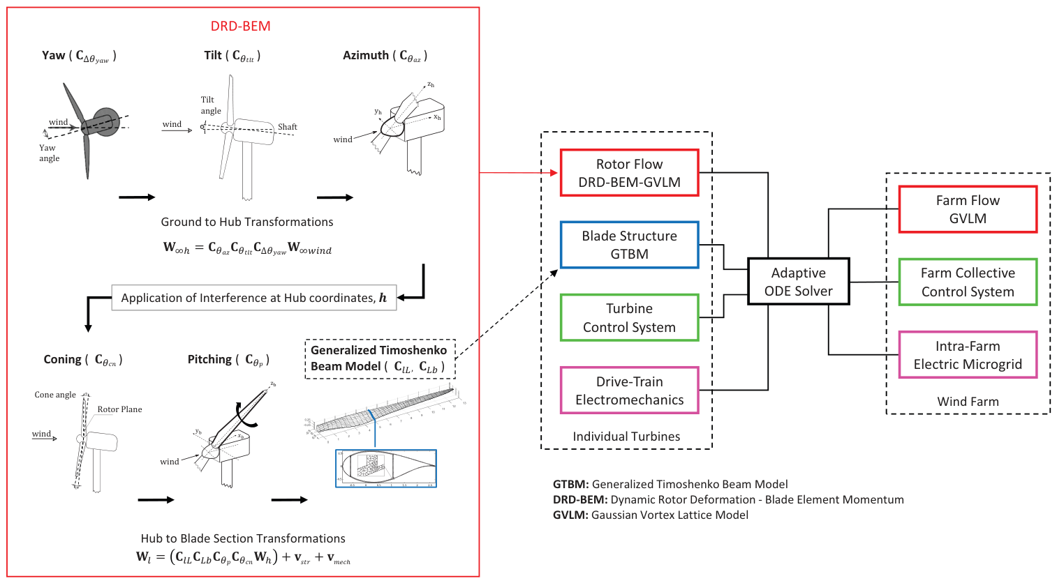
Figure 1 shows a flow chart of the CODEF modular setup, a schematic presentation of the modules related to evaluating blade structure response (GTBM) and the aeroelastic blade dynamics (DRD-BEM), and the set of orthogonal-matrix operators transforming velocities and forces over the successive coordinate systems involved in the DRD-BEM’s calculations. The Gaussian Vortex Lattice Model (GVLM) is also shown and briefly described in this section to illustrate the broader context of the CODEF simulation environment, although the capacities of the GVLM module were not required for this study.

CODEF simulates the coupled multi-physics aspects of wind turbine operation, by performing time-marching evaluations of a multivariable ODE framework of modules, comprising nonlinear, variable order algorithms which describe dynamics governing each physical facet of the problem. CODEF’s modular structure contains submodules for the simulation of rotor flow, blade structure, elecromechanical control, and much more, modeling wind turbine behaviors for an individual turbine, or even multi-turbine flow interactions computed with the GVLM.

Solutions are computed efficiently in stabilized, adaptive time steps, by regulating the local truncation error at each evaluation in time with respect to the collective equations which govern the various independent submodules of the multi-physics problem. CODEF’s unique modular, and inter-related structure is crucial for accurately modeling complex wind turbine aero-elasto-inertial behaviors which are the core subject of this study.

The GTBM submodule of CODEF is used to represent the real-time deformations of blade structure due to aerodynamic loading conditions and control actions. Via a special implementation of the techniques originally proposed by Hodges, Yu, and their collaborators [39,40,41], the blade’s instantaneous deformed configuration is modeled assuming the blade as a complex beam. This method cleverly economizes the computational cost of this evaluation by reducing the three-dimensional problem of the blade structural response into a nonlinear, one-dimensional series of computations performed on the equivalent beam, solved in time steps synchronized with the collective ODE framework of the CODEF solution.

The GTBM dimensional reduction is achieved via a pre-solved series of finite-element problems defined on two-dimensional planes at cross-sections along the full span of the blade. During this process, the blade equivalent-beam model is constructed, which has a fully-populated 6 × 6 stiffness matrix written in terms of the classic variables of the Timoshenko beam theory. However, instead of just the six basic uncoupled stiffnesses of the classic theory, this matrix also includes stiffness coefficients for all coupled deformation modes (like, for instance, the bend–twist modes, the stretch–twist mode, the bend–bend mode in two perpendicular axis, etc.).

In terms of its internal operation, GTBM differs from the classic Timoshenko approach in that it disregards the assumption that the beam cross-sections remain plane during deformation. Instead, the instantaneous warped configuration of each beam deformed section is mapped using a two-dimensional finite-element mesh. By interpolating the actual beam section warp, the aforementioned cross-sectional pre-solutions produce the 6 × 6 complete stiffness matrices for each section along the span of the blade equivalent beam.

For a more in-depth description, Ponta et al. [29], and the references within, provide further reading on the GTBM processes, and also its integration into the global context of the CODEF suite for the simulation the rotor’s aeroelastic dynamics.

The DRD-BEM module in CODEF is responsible for the computation of transient aerodynamic forces acting on each blade section. To accommodate for the complex and time-changing geometry of the wind turbine blade, and the effect of the instantaneous attitude of the blade airfoil sections with respect to the incoming flow, the DRD-BEM transforms the wind velocity vector, described in the “ground” (or geographical) coordinate system, ${{\mathbf{W}}_{\infty }}_{wind}$, into the wind velocity vector described in the instantaneous coordinate system of each blade section, ${\mathbf{W}}_l$. This is done via a series of products involving orthogonal-matrix linear operators. The steps of this product sequence are shown schematically in Figure 1. This sequence also includes the introduction of axial and tangential induction factors, which are applied to account for the turbine’s decelerating interference. The final step is adding the instantaneous relative velocities introduced by the blade structural vibrations, ${\mathbf{v}}_{str}$, and the actions of mechanical devices like main shaft rotation and the yaw and pitch mechanisms, ${\mathbf{v}}_{mech}$.

After the flow velocity on each blade section is determined, aerodynamic loads can be computed based on the lift and drag coefficients of each airfoil-shaped cross section in their instantaneous angle of attack vs. the incoming flow. Then, the same sequence of linear operators could be used in the inverse order to project the lift and drag components back onto the hub coordinate system. Rotor thrust and torque are determined by taking the axial and tangential projections of the hub forces acting on the blade root and adding them together, with power coming from the product of torque and the hub’s rotational speed.

The GTBM evaluations of the instantaneous deformed blade configuration are fed into the DRD-BEM module to accurately project the incoming wind vector onto the instantaneous attitude of the blade sections in the deformed state. That is, these two submodules simultaneously inform each other through the CODEF main framework to create a robust representation of the dynamic aeroelastic behavior of the rotor, in which these deformations, and the associated aerodynamic forces are truly represented.

Comprehensive details about the formulae and algorithmic sequence of the DRD-BEM procedure can be found in Ponta et al. [29], including results of DRD-BEM solutions applied to the analysis of wind turbine blade oscillatory dynamics, and validation studies comparing to data from other well-established sources like Jonkman et al. [13] and Xudong et al. [42].

The GVLM module is not used for this particular study, but will still be briefly described to give greater context for the definition of the CODEF simulation environment and the overall capacities of the multi-physics suite. The GVLM creates a representation of the wake’s vortex-lattice structure by using Gaussian-core vortex filaments, which are shed at elements along the blade’s span, to form a representative vortex-filament lattice which propagates downstream and interacts with other turbine rotors within the farm, and with their wakes.

As an improvement to the singularity representation of the Biot–Savart law used in previous vortex-lattice models, the filament cores of the GVLM have a Gaussian distribution of vorticity. This results in a much more realistic representation of viscous decay with time, and more accurate projections of induced velocity at locations near to the filament core, which substantially improves the fidelity of GVLM in the representation of the complex vortex dynamics phenomena found in turbine-wake evolution.

For a more thorough description of the GVLM module, the reader is referred to Baruah and Ponta [31], who include a mathematical derivation and numerical implementation within CODEF. Baruah and Ponta [31] also show validation tests comparing GVLM results vs. LiDAR measurements of actual wake velocity patterns from Herges et al. [43], taken at the SNL’s Scaled Wind Farm Technology (SWiFT) facility in Lubbock, Texas [44,45,46].

Additional information related to free-vortex-lattice techniques can be found in Strickland et al. [47], Cottet and Koumoutsakos [48], Karamcheti [49], and Baruah and Ponta [31]. More information on the Gaussian-core vortex theory could be found in Ponta [50], Lamb [51], Batchelor [52], Trieling et al. [53], Flór and van Heijst [54], and Hooker [55].

3. Fundamental Aspects of the ROC and the Gust-Pulse Technique

The work to be discussed in this paper is part of an ongoing series of studies related to the notion of the ROC and the gust-pulse technique, and extends across several previous articles. Interested readers are encouraged to refer to these for a complete understanding of the work so far; see Jalal et al. [30], Ponta et al. [32] Yates et al. [33], and Yates et al. [34]. To ensure this article is self-contained, a brief overview of the fundamental aspects of the ROC and the controlled gust-pulse technique shall be given here, followed by a concise review of the typical vibrational modes previously observed in the turbine operational regimes which exhibit a stable oscillatory response.

3.1. The Gust-Pulse Technique

The first aspect of the ROC that will be discussed is its use of gust pulses mounted on a uniform steady-state wind flow of characteristic velocity, WS. These gust pulses are intended to replicate scenarios that real-world wind turbines will experience. Several sources for these gusts were considered in the beginning, such as those caused by: blade rotation through variable flow fields; changes in the time signal of wind velocity, wind direction, wind shear and veer; and those caused by turbine control actions such as blade pitching, nacelle yawing, or variable rotational speed operation.

Ultimately, the input chosen to reproduce the effects of real pulses were pulses generated by changes in the time signals of wind velocity, as they induce the same behavioral response on the rotor’s oscillations. These pulses were classified into three categories based on the timespan of the pulse, since timespan proved to be the most significant factor when characterizing the resulting turbine response behavior. These three categories are classified in terms of the comparison between the relative timespan of their gust pulse and the period of the slowest blade oscillatory mode which is the first bending mode in the rotor’s axial direction (corresponding to ${\mathrm{x}}_{\mathrm{h}}$ in Figure 1).

The first type belongs to the Short pulse category. These gust pulses exhibit a short enough timespan where the pulse ends before there is enough time for the turbine blades to reach their first bending oscillation peak. Aerodynamic damping has no time to act in this situation, which essentially means that all the gust pulse’s kinetic energy is stored as elastic energy in the blade’s first bending oscillation peak. In this case, it is possible to describe the evolution of the blade’s vibrational energy by following the peaks in the blade deflection signal. This is the reason why Short pulses are the ones used in the energy-based characterization of the ROC technique.

On the other end of the timespan range is the Long pulse category. These gust pulses are considered long due to having a long enough timespan such that the energy from the pulse is gradually applied to the blades, allowing the blades to simultaneously absorb and dissipate the energy via aerodynamic damping. This causes these types of pulses to induce only small, even negligible, oscillations.

The third category is the Transitional pulses, which lays in between the previous two. These gust pulses are considered long due to having a long enough timespan such that the energy from the pulse is gradually applied to the blades, allowing the blades to simultaneously absorb and dissipate the energy via aerodynamic damping. This results in only part of the pulse energy being stored in the blade as elastic energy. For Transitional-type pulses, the peak bending deflection is not negligible, as it was with the Long-type pulses, but it is significantly less intense than those associated with Short-type pulses, and their effects are not critical. Further details on the study of these three types of gust pulses can be found in Jalal et al. [30] and Ponta et al. [32].

For the series of works on the ROC, including the present one, several pulses in the Short category were used. For example, one of the short pulses used has an amplitude of 0.5 m/s, representing a 0.5 m/s increase in wind velocity which rises and falls in value back to the background speed of WS over a total timespan of 0.2 s. Several other pulses with different combinations of amplitude and timespan were used. These were applied on a series of wind flows of WS values distributed all over the range of the turbine operational wind speeds. Each operational scenario was defined by the particular combination of WS and the turbine rotational speed. The latter is reported in terms of the tip speed ratio (TSR), a classic non-dimensional parameter used in the design and control of modern utility-scale wind turbines. The TSR is defined as the ratio between the tangential speed of the blade tips and the average speed of the undisturbed incoming wind [27,28], in this case, WS itself.

3.2. Energy-Transfer Characterization

The second aspect of the ROC technique to be described is the energy-transfer characterization. This approach applies controlled Short-category gust pulses in varying combinations of timespan and amplitude to a background steady-state wind stream of a specific velocity WS. The resulting axial blade deflection time signals are then computed. The blade deflections in the direction of the rotor’s axis are measured from the “reference” deflection which corresponds to the one induced by the steady-state wind WS.

Within the “reduced-order” framework of the ROC, the rotor is modeled as a classic spring–mass–damper oscillatory system. In this model, the blades behave similar to a leaf-spring where the flexing deformation occurring in the rotor’s axial direction, with an attached mass and a dashpot element that represents the aerodynamic damping effects experienced by the blade.

In the context of wind turbine blade vibrational dynamics, the axial deflection (also referred to as “Flapwise”), $U_{hx}$, constitutes the dominant deformation mode. This mode absorbs the most elastic deformation energy due to the blade’s high flexibility observed in this particular direction. While the other deformation modes are present in the oscillatory response, like the tangential mode (also called “Chordwise”), and the torsional modes, they are not dominant in typical operational conditions (see Yates et al. [33] for more details). This is the reason why the ROC technique uses the axial deflection as its single degree of freedom in the reduced-order representation. In a similar manner, aerodynamic forces acting in the axial direction are by far the dominant mechanism generating damping, with internal friction in the blade’s structural material playing a negligible role in vibrational dissipation.

As previously mentioned, the kinetic energy of an individual gust pulse of the Short type is almost entirely absorbed by the rotor as a spring–mass oscillatory system. The vibrational mechanical energy stored in the rotor at any time can be quantified by evaluating the amount of elastic energy at each one of the peaks in the axial blade deflection signal, with an enveloping curve being used to trace the change in peak height over time. From this analysis, a direct correlation could be established between the elastic energy accumulated during the blade’s deformation and the kinetic energy contained in the gust pulse that initiated the oscillation signal.

There is a wide range of WS and TSR combinations where the rotor’s oscillatory response is stable, that is, the oscillations induced by a gust-pulse decay with time. Jalal et al. [30] and Ponta et al. [32] found that, when the turbine operates inside that Stable region, the kinetic energy per unit area delivered by the gust pulse on the rotor’s disk surface, $PulseEner$, can be used as a normalization factor for the axial blade deflection, $U_{hx}$.

Observing the Normalized Blade Deflection (NBD), defined as ${\displaystyle \frac{U_{hx}}{PulseEner}}$, of the oscillatory response for all individual pulses, reveals that the signals collapse into one nearly identical plot. This collapse is observed not only in the signal’s frequency but, most importantly, in the enveloping curve that defines the oscillatory decay of the signal. The rate of decay of the NBD was found to be determined by aerodynamic damping, and depending solely on the operational regime (defined by the combination of background wind speed, WS, and rotor tip speed ratio, TSR), regardless of the the specific characteristics (amplitude and timespan) of the short pulse applied (see Jalal et al. [30] and Ponta et al. [32] for more details). This leads to a unique characterization of the oscillatory response of the rotor which only depends on the operational parameters, not on the features of the gust pulse that induced the vibration.

In the context of the present work, this means that all examples of rotor vibrational response presented in this paper (related to one pulse in particular) are also representative of the rotor response to any other short gust pulse applied in the same operational conditions defined by that WS-TSR combination.

Expanding on those previous works, Yates et al. [33], and Yates et al. [34] reported comprehensive details of the nature of the several stability behaviors. In particular, the loci of Stable and Unstable regions in the shape of TSR vs WS Stability Map. Yates et al. [33] also demonstrated the universal nature of the ROC by reporting its results in terms of non-dimensional parameters. This means that ROC results could be applied to rotors of any size as long as they share a similar blade shape design, and a similarity of blade structural construction.

3.3. Single-Mode and Two-Mode Stable Responses

The reduced-order nature of the ROC is based on the fact that the elastic energy that remains stored within the blade at each instant is evaluated solely based on the blade’s deflection in the first axial (also called “Flapwise”) mode of movement. That is, the characterization is performed in a reduced-order manner.

As mentioned before, this simplified formulation produces accurate evaluations of oscillatory behavior, while also substantially economizing computations so that they can be performed in real time with the control system. The first mode of oscillation (Mode-1) remains largely dominant in operational conditions with a stable rotor response, therefore making this Single-Mode characterization an adequate description for the rotor vibrational behavior in the reduced-order sense.

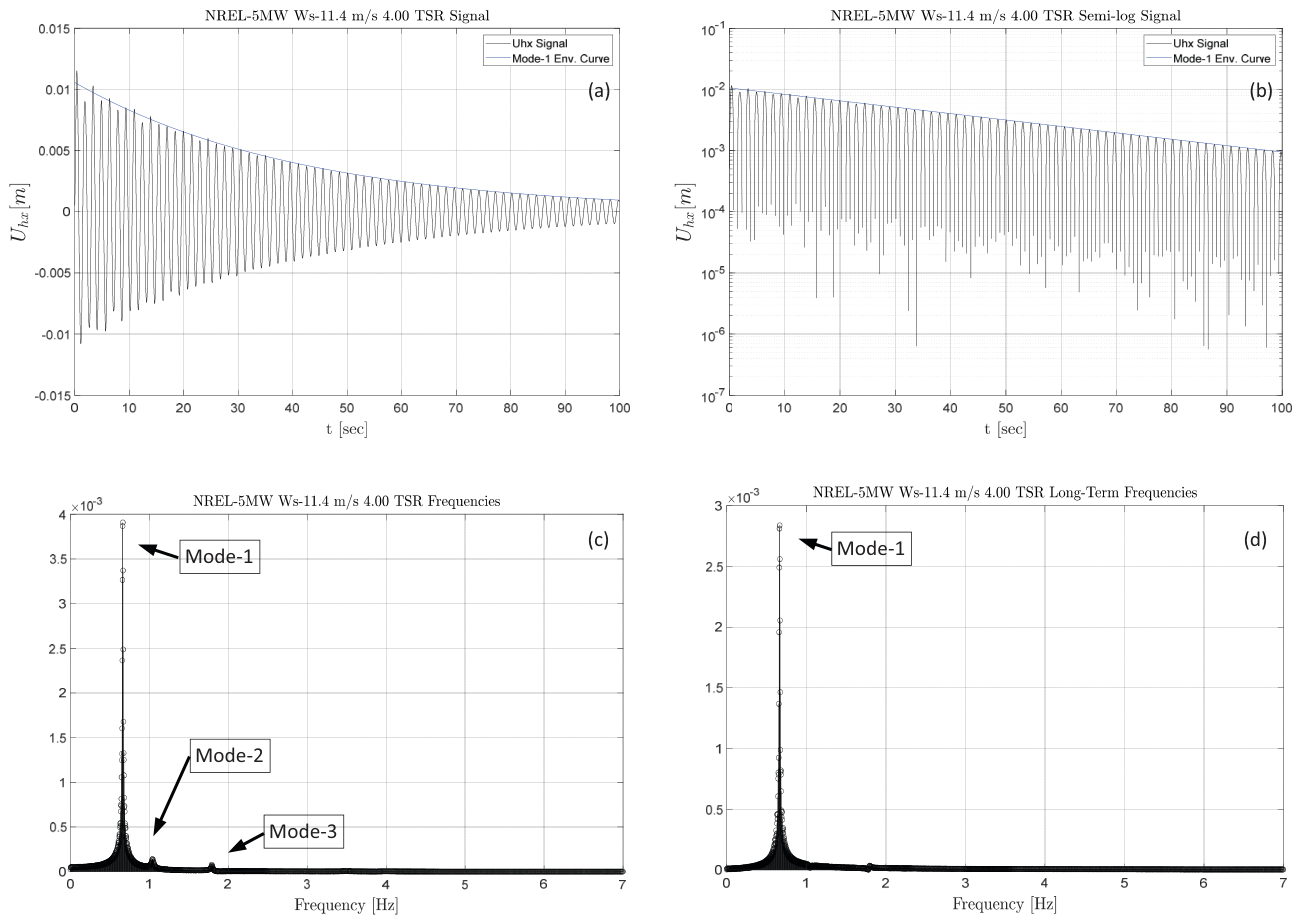
To illustrate this point, Figure 2 shows an example of the typical blade oscillatory response of an NREL-5MW-RWT turbine excited by a gust pulse when operating in the Stable region, for a case where the vibrational response is entirely dominated by Mode-1.

Figure 2a, shows the time evolution of the axial blade deflection, $U_{hx}$, which exhibits a singular value of exponential decay, ${\lambda }_1$, for the entirety of its duration (0 to 100 s). Figure 2b shows the semi-log plot of that same signal, where the exponential nature of the oscillatory decay can be readily seen in the linear form of the enveloping curve. Figure 2c shows the spectrum of the Single-Mode oscillatory signal in its entire duration, and Figure 2d shows the spectrum in the long-term stages of the signal (in this case, from 20 to 100 s).

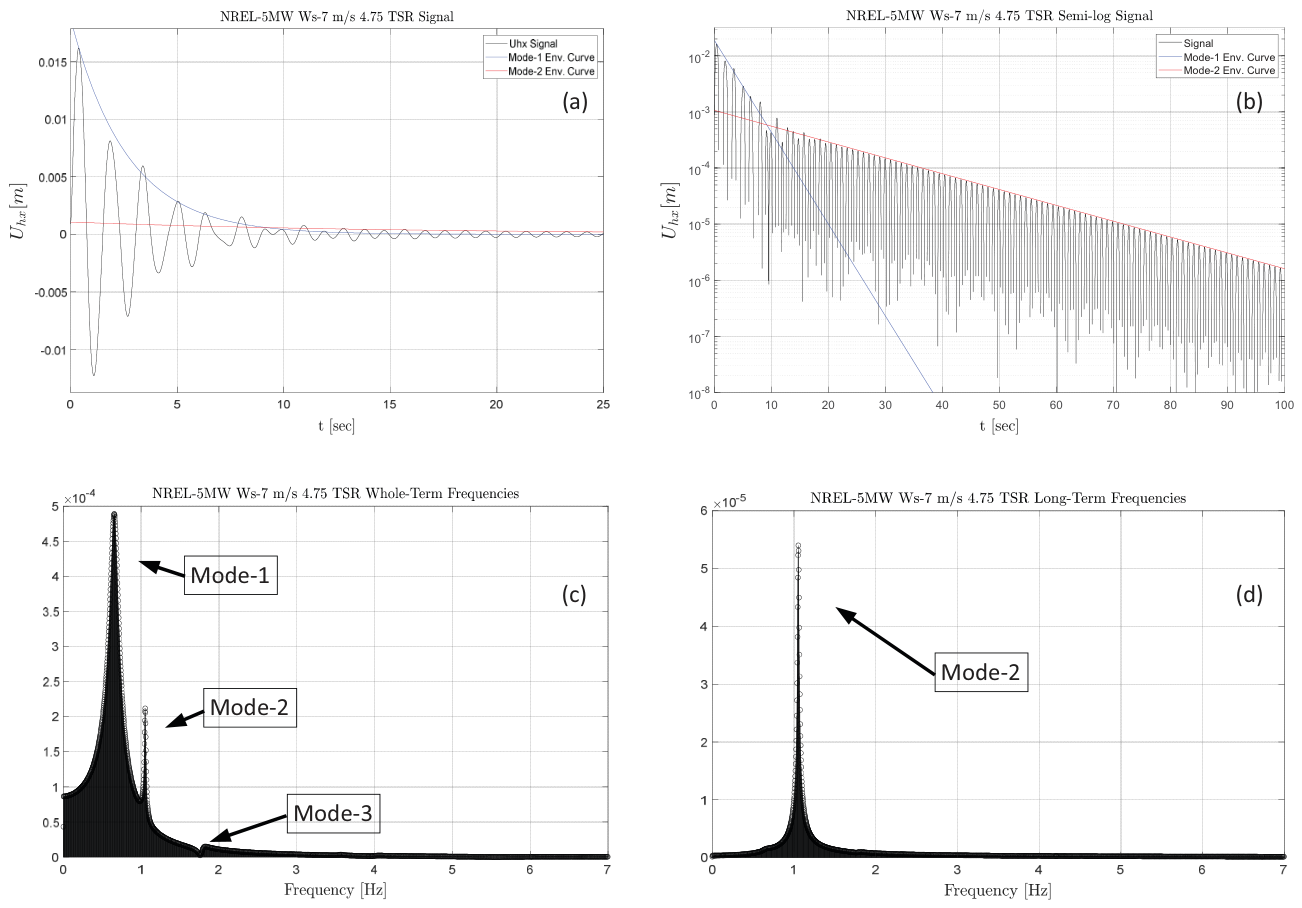
The other example of behavior that is frequently observed in the Stable region is the Two-Mode decaying vibrational response, which is illustrated in Figure 3. The time evolution of the axial blade deflection for this behavior is shown in Figure 3a, where the presence of second mode of vibration, Mode-2, manifests visually as an alteration in the shape of the signal (particularly visible in the early oscillation cycles).

In the authors’ previous works [30,32,33,34], it has been observed that all blade oscillatory modes are coupled in nature. This feature is directly inherited from the fact that wind turbine blades, as complex beam structures, exhibit modes of deformation that are coupled in nature too (e.g., bend–twist, stretch–twist, the bend–bend two perpendicular axes). As was mentioned in Section 2, the GTBM module of CODEF is capable of detecting those coupled modes of deformation present in the oscillatory response. This is the case for Mode-2, which, while clearly visible in the axial deflection signal ($U_{hx}$ in Figure 3a), it is primarily tangential (or “Chordwise”) in nature, and it is dominant in the tangential deflection $U_{hy}$ (corresponding to the ${\mathrm{y}}_{\mathrm{h}}$ direction in Figure 1).

Characteristically, Mode-2 has a significantly lower intensity than Mode-1, but it also shows a lower rate of decay, ${\lambda }_2$. This makes the Mode-2 vibrational component more persistent in the long term, as it is slower to dissipate. Figure 3b shows the semi-log plot of this Two-Mode signal, illustrating the interplay between Mode-1 and Mode-2, as well as their relative rates of decay.

Figure 3 also illustrates an occasional feature occurring in the Two-Mode behavior, which is the presence of a usually weaker third oscillatory mode, Mode-3, which is, like Mode-1, axial (or “Flapwise”) in nature. In most of the Stable region, Mode-3 is found to be significantly lower than Mode-2, appearing only as a slight alteration in the signal in the time range around the intersection of the straight lines representing the Mode-1 and Mode-2 enveloping curves in Figure 3b semi-log plot.

The relative intensity of the three oscillatory modes could be better appreciated by comparing the spectra for the Single-Mode case, shown in Figure 2c, and the Two-Mode case, shown in Figure 3c, as well as their respective statuses in the long-term response shown in Figure 2d and Figure 3d. As an example, in the case of the NREL-5MW-RWT, Mode-1 shows a characteristic frequency, $f_1$, between 0.65 and 0.70 Hz (depending on the specific operational conditions), and Mode-2 and Mode-3 show $f_2$ and $f_3$ frequencies of 1.05 Hz and 1.76 Hz, respectively.

These three modes, typically observed within the Stable region, were initially documented in Jalal et al. [30], and later confirmed by findings reported in Ponta et al. [32] and Yates et al. [33]. This current work and the aforementioned preceding works combine to form an expanding collection of numerical experiments elucidating these behaviors which manifest in a diverse range of turbine designs, sizes, operational conditions, rotational regimes, wind speeds, and pitch and stall control scenarios.

In very few situations (usually located at the high end of the WS range in the Stable region), there is a variation of the Single-Mode behavior, which shares some features with the Two-Mode behavioral type. In these rare situations, Mode-1 dominates the vibrational response all over its duration, like in the Single-Mode case. However, there is a small contribution of Mode-2 and Mode-3 in the initial stages, as is observed in the Two-Mode response. The difference is that Mode-2 vanishes rapidly, instead of decaying slowly as in the typical Two-Mode case. The result is that now the long-term response is dominated by Mode-1 instead of Mode-2, with a small contribution of Mode-3 remaining in the background.

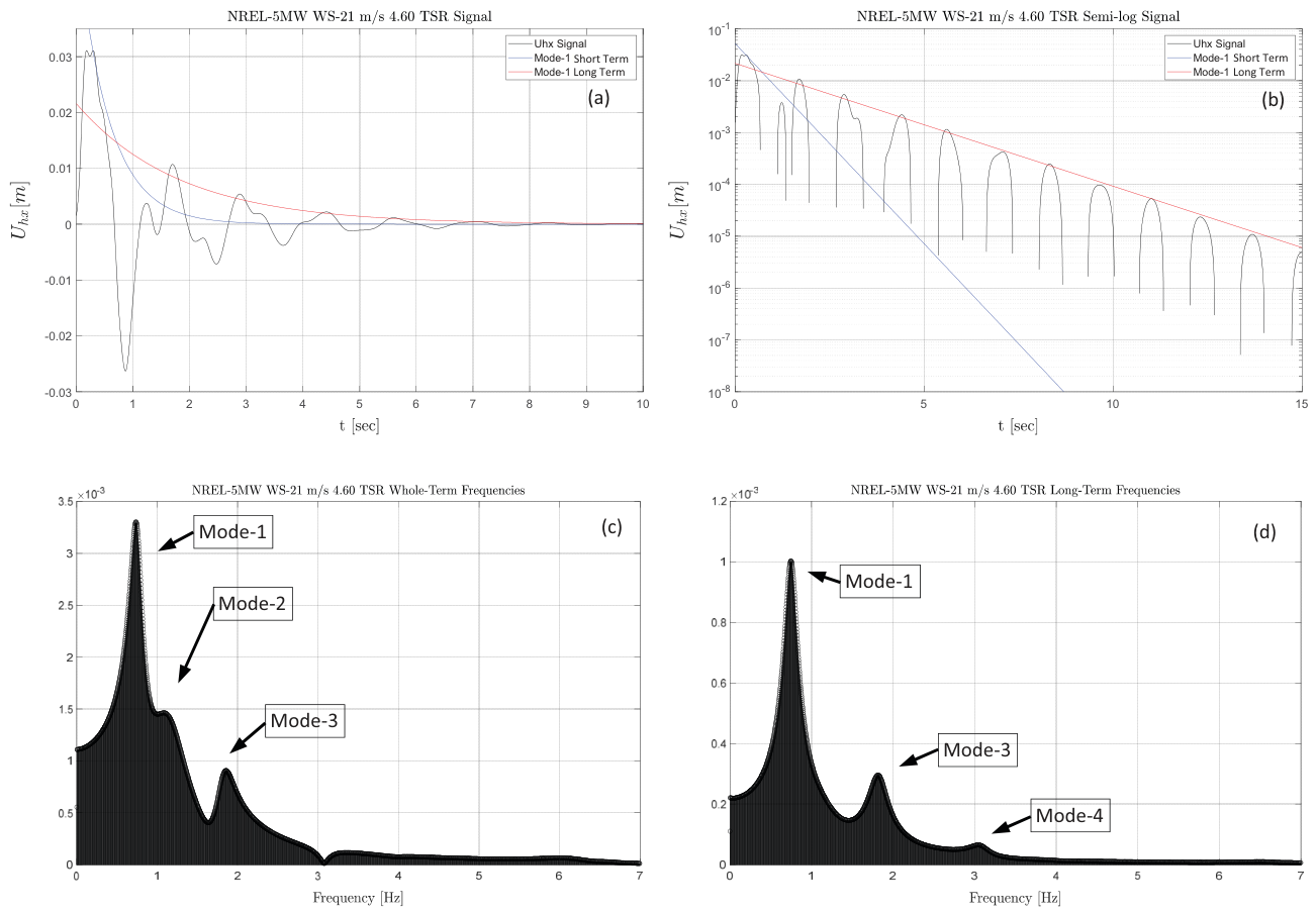
Figure 4 shows an example of this rare variation of the Single-Mode behavior: a response signal for a NREL-5MW-RWT turbine operating in the Stable region, at WS = 21 m/s and TSR = 4.60. As before, Figure 4a, shows the time evolution of the axial blade deflection, Figure 4b shows the semi-log plot of that same signal, Figure 4c shows the spectrum of the oscillatory signal in its entire duration, and Figure 4d shows the spectrum in the long-term stages.

An interesting feature observed in this type of Single-Mode behavior is that the rate of decay of Mode-1 decreases after Mode-2 vanishes. This change could be observed in the difference between the shape of $U_{hx}$ enveloping curve in the short term, indicated in blue in Figure 4a,b, vs. the one in the long term, indicated in red.

The behavior observed in all the previous studies confirmed that Mode-1 is dominant in the Stable region, even in the presence of Mode-2 and Mode-3, supporting the concept of using the Single-Mode ROC technique to predict the dominant aspects of the rotor’s oscillatory response when wind turbines operate in the Stable region.

There are two other modes that have been observed at the external limits of the Stable region, close to or at the boundary with the Upper Unstable Region (UUR) observed in the high TSR ranges of the aforementioned Yates et al. [33] Stability Map. These two modes are called Mode-4 and Mode-5. For the case of the NREL-5MW-RWT turbine, Mode-4 has a characteristic frequency, $f_4$, between 2.8 and 3.3 Hz (depending on the specific operational conditions), and Mode-5 a characteristic frequency, $f_5$, around 5.8 Hz.

Mode-4 and Mode-5 are torsional-dominant, and they are generally negligible throughout the core of the Stable region, only emerging at the said boundary. Due to the aforementioned bend–twist coupling of the blade deformation modes, Mode-4 and Mode-5 also manifest themselves in the axial blade deflection plots in those borderline situations close to the stability limits. We shall revisit these modes, and their locus in the Stability Map in our discussion on Multi-Modal Response behavior in Section 4.2 and Section 4.3.

4. Forms of Multi-Modal Oscillatory Response

The present work will expand the knowledge about the nature of stability regions and the boundaries separating them, particularly, in operational conditions defined by WS-TSR combinations that trigger a Multi-Modal Response (MMR) mainly observed in regions located at the stable boundary zone of the Stability Map. This will provide valuable information about rotor stability behavior in extreme turbine operational conditions which were previously unexplored.

In this section, three different categories of Multi-Modal vibrational response will be described:

• Activated Mode-3 Stable Response, discussed in Section 4.1
• Hybrid Bend–Twist Mode and Mode-1b Responses, discussed in Section 4.2
• Characteristic Modes of the Upper Transitional Boundary, discussed in Section 4.3

In each case, selected examples of the time signal for the axial blade deflection, $U_{hx}$, will be shown, together with plots of the corresponding spectra for the whole duration of the $U_{hx}$ time evolution and its behavior in the long term. Section 4.3 will also present an expanded version of the previous Yates et al. [33] Stability Map.

4.1. Activated Mode-3 Stable Response

While typically a minor presence in most situations within the Stable region, there is a zone of TSR values where Mode-3 is much more active. This activated Mode-3 zone, ActM3, covers a band of values near $\mathrm{TSR}=5.00$, whose width and location varies slightly depending on the corresponding WS. In the ActM3 zone, the presence of Mode-3 in the modal composition reaches the point where it might become the dominant mode in the long-term period of the oscillatory response, after Mode-1 (dominant in the initial stages) vanishes.

This is in contrast to the most typical Single-Mode and Two-Mode behaviors observed in the Stable region described in Section 3.3, where the long-term response is dominated either by Mode-1 or by Mode-2, respectively.

Even in those rare variations of the Single-Mode behavior, like the one shown in Figure 4, Section 3.3, Mode-3 is not dominant in the long term. That is, in those situations, Mode-2 and Mode-3 are present in the initial stages, but after Mode-2 rapidly vanishes, the contribution of Mode-3 is still small vs. Mode-1’s. Hence, those cases do not belong to the ActM3 category described here.

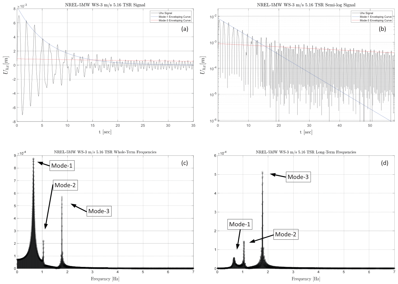
Figure 5 shows an example of the typical response observed in the ActM3 behavioral type, for an NREL-5MW-RWT rotor operating in the Stable region at WS = 3 m/s and TSR = 5.16. Figure 5a shows the time evolution of the axial blade deflection, Figure 5b shows the semi-log plot of that same signal, Figure 5c shows the spectrum of the oscillatory signal in its entire duration, and Figure 5d shows the spectrum in the long-term stages.

In this example of ActM3 response, Mode-1, Mode-2, and Mode-3 are present in the initial stages, in a manner that resembles the Two-Mode behavior described in Section 3.3. However, after Mode-1 decays, the long-term response is essentially dominated by Mode-3 instead of Mode-2, with Mode-1 and Mode-2 playing a minimal role.

Another feature of this variation of the ActM3 type is that the exponential rate of decay of Mode-3, ${\lambda }_3$, is relatively low compared with the decay rates of Mode-2 observed in the long-term stages of the Two-Mode behavior described in Section 3.3. This makes Mode-3’s small residual vibrations more persistent, taking longer to dissipate.

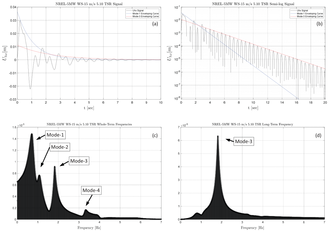
Figure 6 shows another example of the ActM3 behavioral type, in this case, involving an NREL-5MW-RWT rotor operating in the Stable region at WS = 15 m/s and TSR = 5.10.

As in previous examples, Figure 6a shows the time evolution of the axial blade deflection, Figure 6b shows the semi-log plot of that same signal, Figure 6c shows the whole-term spectrum of the oscillatory signal, and Figure 6d shows the spectrum in the long-term stages.

In this ActM3 example, the first three modes are present in the initial stages, with Mode-1 being dominant, along with the addition of a minor contribution from the first torsional mode, Mode-4. After those initial stages are passed, Mode-3 entirely dominates the response, with the remaining modes vanishing completely.

In this type of ActM3 case, Mode-3’s decay rate values are larger, and its residual vibrations dissipate faster than in the previous ActM3 example shown in Figure 5.

4.2. Hybrid Bend–Twist Mode and Mode-1b Responses

At the higher end of wind speeds, a different behavior is seen in terms of the vibrational modes that are activated. Starting at WS values around 11 m/s, there is an incipient appearance of Mode-4 and Mode-5 in the frequency content of both the initial stages and the long-term responses.

The contribution of these torsional-dominant modes starts to become progressively more prominent as WS increases, until it reaches values comparable to the more usual contributions of Mode-2 and Mode-3. Because of the mixed nature of this flexo-torsional oscillatory behavior, it will be referred to henceforth as the Hybrid Bend–Twist, HyBT, behavioral type.

As was discussed in Section 3.3, all modes of blade deformation are coupled in nature. Hence, even though Mode-4 and Mode-5 are predominantly torsional, they appear in the axial bending oscillatory signals due to bend–twist structural coupling, and become part of the axial bending elastic energy analysis at the core of the ROC technique (see Section 3.2).

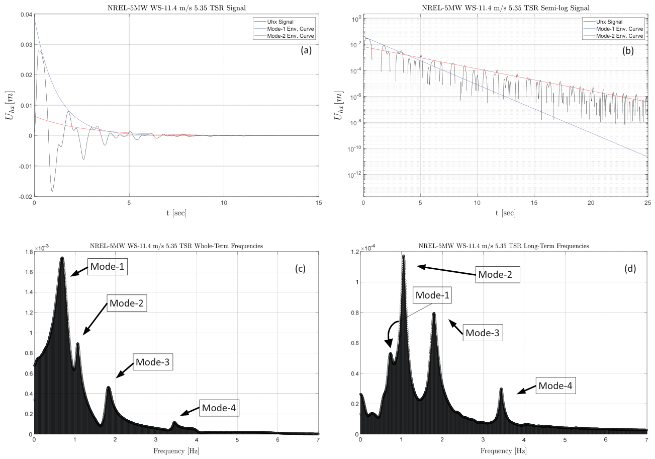
Figure 7 shows an example of incipient emergence of the HyBT behavior for the case of an NREL-5MW-RWT rotor operating in the Stable region at WS = 11.4 m/s and TSR = 5.35. Figure 7a shows the time evolution of the axial blade deflection, Figure 7b shows the semi-log plot of that same signal, Figure 7c shows the spectrum of the oscillatory signal in its entire duration, and Figure 7d shows the spectrum in the long-term stages.

Even though in this example Mode-1 is clearly dominant in the initial stages (as in most Two-Mode situations in the Stable region), with Mode-2 and Mode-3 being the most relevant in long-term response, Mode-4 now persists beyond the initial stages and well into the long-term period.

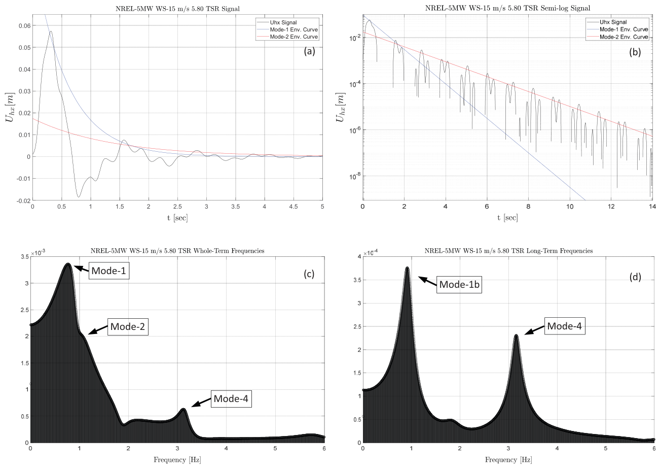
As we move into higher WS values, the HyBT behavior becomes more noticeable. Figure 8 shows another example of HyBT response, in this case involving an NREL-5MW-RWT rotor operating in the Stable region at WS = 15 m/s and TSR = 5.80.

As before, Figure 8a shows the time evolution of the axial blade deflection, Figure 8b shows the semi-log plot of that same signal, Figure 8c shows the spectrum of the oscillatory signal in its entire duration, and Figure 8d shows the spectrum in the long-term stages.

The response shown in Figure 8 represents a moderate example of the HyBT behavior. It also serves the purpose of introducing a new feature that becomes very prominent in strong-HyBT cases observed at higher values of WS. This feature is connected with the “locking” of Mode-1 and Mode-2 into a single mode of vibration with an intermediate characteristic frequency.

This locking process can be observed by comparing the whole-term spectrum shown in Figure 8c vs. it long-term counterpart in Figure 8d. In the initial stages of the oscillatory response, Mode-1 and Mode-2 are essentially separate modes. Due to the higher amplitude of the deflection signal in the early stages, their respective energies are reflected in the whole-term spectrum, with frequencies around 0.65 Hz and 1.05 Hz, respectively.

However, the long term spectrum only shows one single mode in the lower frequency ranges, with an intermediate frequency value around 0.87 Hz.

Given that this new locked mode is now the first mode of response in terms of its frequency, but at the same time, differs from the original Mode-1 by being replacing Mode-1 and Mode-2, it will be referred to henceforth as Mode-1b.

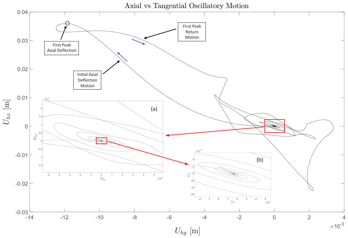
In order to test the hypothesis of the emergence of Mode-1b as a result from the locking of Mode-1 and Mode-2 into a single mode, and to illustrate some details about the physics behind this phenomenon, Figure 9 shows a depiction of the combined blade deflection motions in the axial and tangential directions, $U_{hx}$ and $U_{hy}$, for the case of an NREL-5MW-RWT rotor operating in the Stable region at WS = 21 m/s and TSR = 4.80.

The winding curve shown in black in Figure 9 represents the trajectory described by the combined motions of the blade’s tip in the ${\mathrm{x}}_{\mathrm{h}}$–${\mathrm{y}}_{\mathrm{h}}$ axes (see Figure 1). In this plot, the origin is set at the Neutral position of the blade’s tip in the steady-state conditions before the gust pulse is applied.

The trajectory curve starts at the origin, with the initial windward motion of the blade tip toward the first peak of axial deflection which follows the application of the gust pulse (its direction is indicated in the figure with a blue arrow). After reaching the point of maximum axial deflection, shown in the figure as a blue circle, the return motion in the leeward direction starts (also indicated in the figure with a blue arrow).

From then on, the blade continues its oscillation by moving primarily along the axial direction, with a lower displacement in the tangential direction (for clarity purposes, the scale of both axes in the figure is represented differently).

The main plate of Figure 9 shows the whole trajectory since the start of the motion, while the insets in Figure 9a,b show close-up views of the trajectory in successive later stages, as the oscillatory motion decays spiraling down towards the origin.

An observation of the early stages of the blade tip motion clearly shows that the displacements in the axial and tangential directions are not correlated; that is, their frequencies are not synchronized, with the trajectory curve moving in a complex pattern winding around itself. This is consistent with the fact that, as was mentioned in Section 3.3, the axial motion is primarily related to Mode-1, while the tangential motion is primarily related to Mode-2, both of them possessing different frequencies.

However, as the oscillatory motion progresses in time, the trajectory curve switches into an elliptical shape akin to a Lissajous pattern. This indicates that now the axial and tangential oscillatory motions are essentially synchronized into a new frequency, or in other words, that Mode-1 and Mode-2 have merged into a new oscillatory mode: Mode-1b.

The presence of Mode-1b is a characteristic that becomes very prominent in strong-HyBT cases observed at higher values of WS, where the locking of Mode-1 and Mode-2 occurs very rapidly at the initial stages of the oscillatory response.

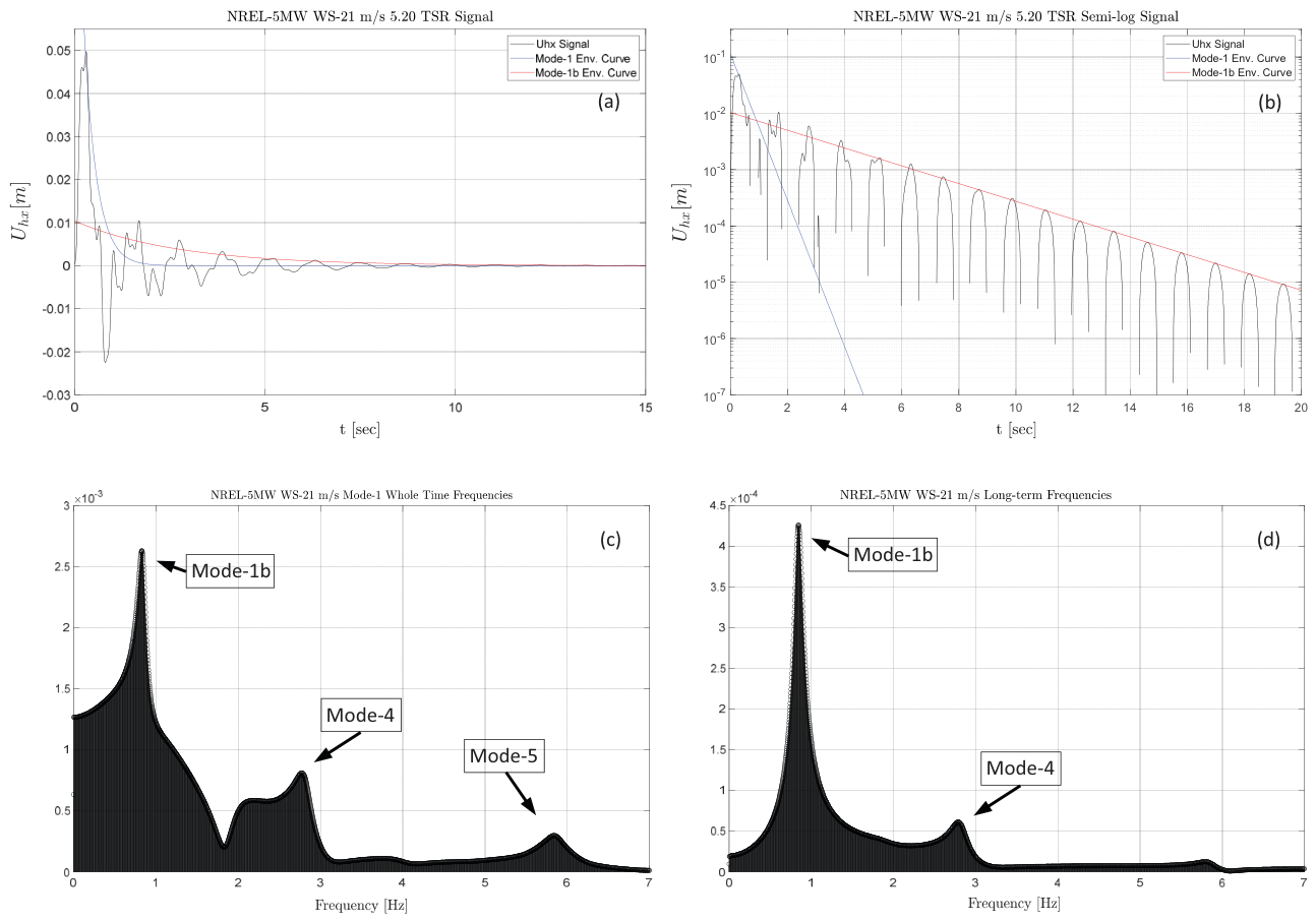
In some situations, the Mode-1/Mode-2 locking occurs fast enough that Mode-1b becomes the dominant feature even in the short term (with some contribution from Mode-4 and Mode-5), and remains the dominant mode in the long term after Mode-4 and Mode-5 decay.

Figure 10 shows an example of this behavior involving an NREL-5MW-RWT rotor operating in the Stable region at WS = 21 m/s and TSR = 5.20. As in previous examples, Figure 10a shows the time evolution of the axial blade deflection, Figure 10b shows the semi-log plot of that same signal, Figure 10c shows the spectrum of the oscillatory signal in its entire duration, and Figure 10d shows the spectrum in the long-term stages.

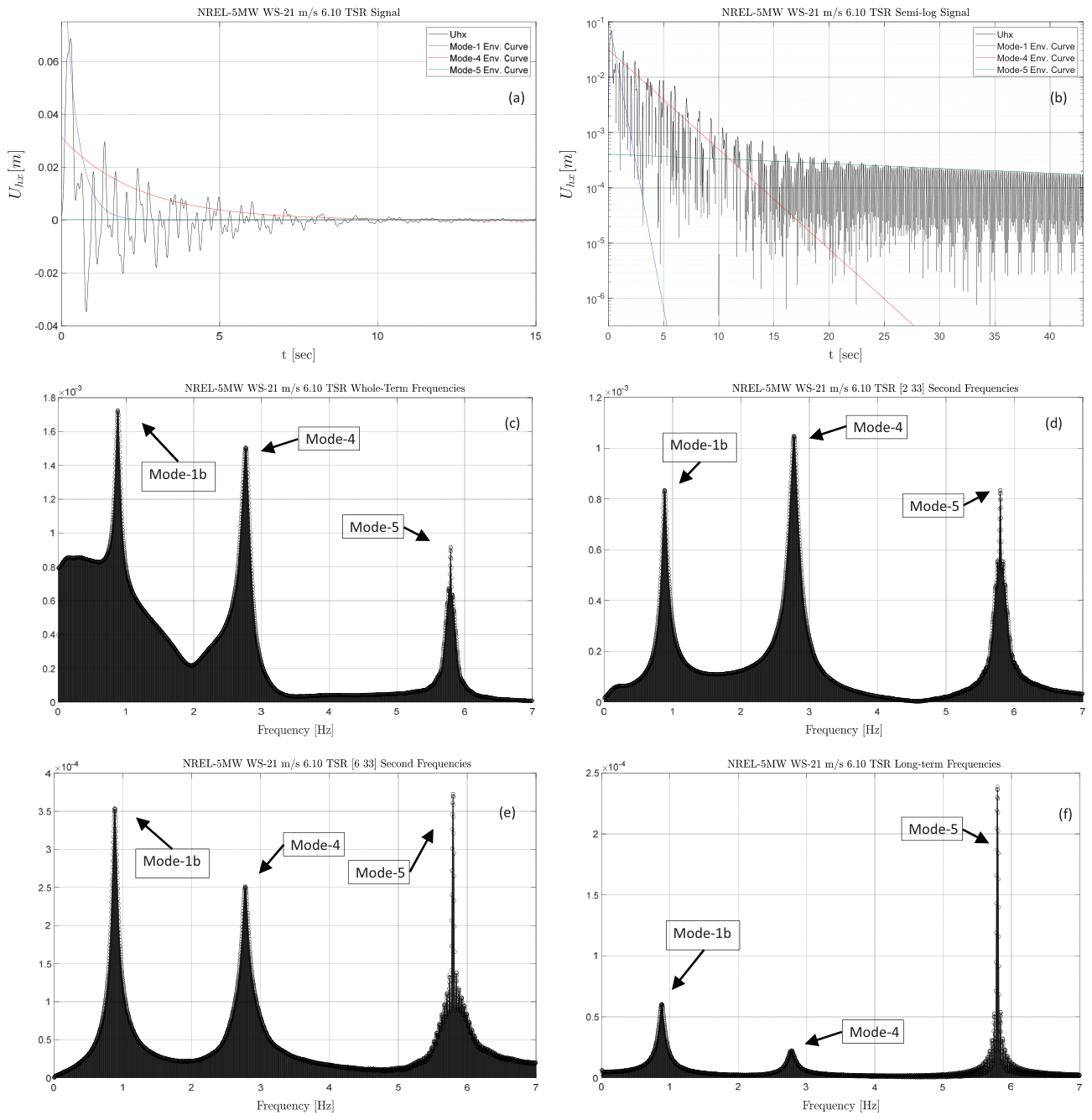
In other situations, usually associated with a combination of high values of WS and TSR, the modal mix becomes very rich. In those HyBT cases, Mode-1b is the dominant feature in the short-to-medium term, until it is superseded by the torsional modes in the long term stages (either Mode-4, Mode-5, or a combination of both).

Figure 11 shows an example of this behavior for an NREL-5MW-RWT rotor operating in the Stable region at WS = 21 m/s and TSR = 6.10. Figure 11a shows the time evolution of the axial blade deflection, Figure 11b shows the semi-log plot of that same signal, Figure 11c shows the spectrum of the oscillatory signal in its entire duration, Figure 11d,e show the spectra in two periods of the intermediate stages, and Figure 11f shows the spectrum in the long-term stages.

As can be observed in the spectra depicted in Figure 11c–f, in these HyBT cases located at the high end of the WS/TSR range of operational conditions, there is a more complex mix of modal distribution. These situations represent the richest examples of Multi-Modal Response, which evolves along different stages of the blade deflection signal, alternating the dominance of each mode present.

In this particular example, the evolution of the frequency content starts with no mode being clearly dominant in the early stages, which is, essentially, a combination of Mode-1b, Mode-4, and Mode-5 sharing the spectrum practically in equal terms, with Mode-1b being slightly higher.

As the response evolves into the intermediate stages, Mode-1b is superseded by the torsional modes, first by Mode-4, with a secondary contribution of Mode-5. This is followed by a decrease in Mode-4 and an increase in Mode-5, which becomes the clearly dominant feature in the long-term stages.

The locus of these high-WS/TSR cases of the HyBT behavior is close to the upper limit of the Stable region in the Yates et al. [33] Stability Map. Characterized by high values of turbine rotational speeds (i.e., high TSR values), this limit is called the Upper Transitional Boundary (UTB). The types of modal response observed at the UTB will be the focus of the following Section 4.3.

4.3. Characteristic Modes of the Upper Transitional Boundary

As was mentioned in Section 1, in their analysis of physical mechanisms of aerodynamic damping, Yates et al. [34] studied the nature of a stability transition taking place at lower values of turbine rotational speed (i.e., low TSR values) in the previous Yates et al. [33] Stability Map. This Lower Transitional Boundary (LTB) marked the switching between the Stable region of the map and the Lower Unstable Region (LUR) [33,34].

Yates et al. [34] determined that the stability change occurring at the LTB was triggered by an inversion in the sign of the exponential rate of decay of Mode-1, ${\lambda }_1$, which went from a positive value to a negative one.

This change was due to a switch in the balance of axial aerodynamic forces acting on the blade along each oscillatory cycle, which altered the net exchange of aerodynamic mechanical energy between the blade, as an oscillatory system, and the wind flow (see Yates et al. [34] for comprehensive details).

In the Stable region, the energy input from the flow into the blade oscillations was negative, dissipating the vibrational energy imparted by the gust pulse. In the LUR, that energy input was positive, amplifying the oscillation amplitude and inducing an unstable aeroelastic condition.

Being the LTB transition related to an expansion of Mode-1 oscillations, in the context of the present paper, we shall refer to it as a Mode-1-Type Instability.

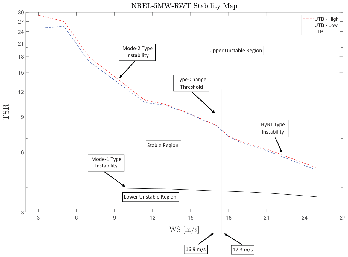
This is in contrast to the two types of instability observed at the locus of the UTB, which are Multi-Modal in nature. In one case, the instability is triggered by an expansion of Mode-2 vibrations, and will be referred to as a Mode-2-Type Instability. In the other case, it is triggered by an expansion of the torsional modes, and will be referred to as an HyBT-Type Instability.

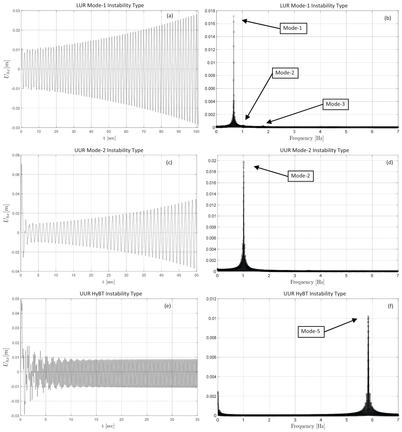
Figure 12 shows selected examples of the different types of unstable behavior for the case of an NREL-5MW-RWT rotor operating in the LUR and in the UUR regions.

Figure 12a shows the time evolution of the axial blade deflection for a typical case of Mode-1-Type Instability, observed in the LUR at WS = 11.4 m/s and TSR = 3.90, while Figure 12b shows the corresponding spectrum of the expanding oscillatory signal, where the dominance of Mode-1 is clearly visible.

Figure 12c shows the time evolution of the axial blade deflection for a typical example of Mode-2-Type Instability, observed in the UTB at WS = 7 m/s and TSR = 18.50, while Figure 12d depicts the corresponding spectrum, showing the dominance of Mode-2.

Finally, Figure 12e shows the time evolution of the axial blade deflection for a typical case of HyBT-Type Instability, observed in the UTB at WS = 25 m/s and TSR = 4.99, while Figure 12f depicts the corresponding spectrum, showing in this case the dominance of Mode-5.

As was mentioned before, the nature of the LTB transition was found to be dominated in its entirety by the Mode-1-Type Instability [33,34]. This is in contrast to the instability types reported here for the UTB.

In the present study, it was found that the lower-WS zone of the UTB is characterized by a Mode-2-Type Instability, while the zone of higher WS values is dominated by an HyBT-Type Instability.

To illustrate this point, Figure 13 shows an updated version of the the previous Yates et al. [33] Stability Map example for the case of an NREL-5MW-RWT rotor, indicating the different instability types characterizing the LTB and the two main sectors of the UTB.

Yates et al. [33] found that the locus of the LTB is very well defined in terms of the thickness of the boundary line, with an almost negligible variation in the transition threshold measured for cases involving several gust pulses of different amplitudes and timespans applied on each particular WS/TSR condition.

This is in contrast to what was observed for the UTB in the present study, where the transition occurs in a band of TSR values for each WS analyzed. The upper and lower limits of the UTB band of values are indicated in Figure 13 as UTB-Low (marked in blue), and UTB-High (marked in red).

For the case of the NREL-5MW-RWT rotor, the threshold marking the change from a Mode-2-Type Instability into an HyBT-Type Instability of the UTB was found to be in a narrow WS band between 16.9 m/s and 17.3 m/s, depending on the amplitude and timespan of the gust pulse used. This is indicated in the figure by vertical lines with their corresponding labels.

5. Conclusions

In this paper we have presented research efforts to expand the application of the ROC technique to predict the emergence of Multi-Modal blade vibrational responses observed in situations characterized by high turbine rotational speeds, and high values of wind flow velocities. In particular, situations which are located at the upper limit of the stable zone in the Yates et al. [33] Stability Map published previously.

This expansion will provide valuable information about rotor stability behavior in extreme (and/or transient) turbine operational conditions at high rotational/high wind speeds, which were previously unexplored, complementing the studies at low rotational speeds presented before. Even though those extreme conditions appear less frequently than the standard conditions found in regular turbine operation, they may pose a threat to the structural integrity of the turbine components, and to their life span because of accumulation of fatigue damage.

Hence, having a simple reduced-order formula like the one provided by the ROC, capable of being solved in real-time, has a substantial value in the context of developing predictive control strategies to maximize turbine energy generation and mitigate fatigue damage. Determining the nature of the boundaries that envelope the stability regions for alternative operational conditions will help to envision potential control scenarios to deal with those situations without risking a control setting that might eventually place the rotor into an unstable oscillatory regime.

Establishing the mix of frequencies of the expected vibrational response excited by gust pulses of different types contained in the wind flow also provides a significant advantage from the point of view of blade geometrical and structural design.

The non-dimensional, size-independent nature of the ROC, already demonstrated in Ponta et al. [32] and Yates et al. [33], makes these results particularly useful, as commercial wind turbines continue to increase in diameter with future designs.

As was mentioned in Section 4.3, the locus of the LTB found by Yates et al. [33] is very well defined in terms of the thickness of the boundary line, which represents a contrast to what was observed for the UTB in the present study, where the transition occurs in a band of TSR values for each WS analyzed.

Even though the width of this transitional band is very narrow (especially in the portions of the UTB surrounding the change in stability type, where it is practically nil), it is still wider than in the LTB case. This could be attributed to the Multi-Modal nature of the incipient instability occurring at the UTB, with multiple modes reacting differently to the gust-pulse shape being activated at different TSR thresholds, which differs from the simpler Single-Mode nature of the LTB. The narrow width of the threshold for the instability type change (from Mode-2- to HyBT-type), observed in the UTB, could also be attributed to the Multi-Modal nature of the UTB, with different modes showing slightly different levels of sensitivity to the shape of the pulse applied.

As an outlook for further work, it may prove beneficial to explore a future extension of this work into the analysis of the oscillatory response during the transient states or rotor angular acceleration, which occur during turbine start-up stages. Those stages, characterized by low rotational speeds (hence, low TSR values), have the potential to alter the typical behavior of the physical mechanisms producing aerodynamic damping. Particularly, the process of interaction between aerodynamic forces during the blade oscillatory motion, which are responsible for generating aerodynamic damping that dissipates vibrational energy.

References

1. NREL. Wind Vision. A New Era for Wind Power in the United States; Technical Report; U.S. Department of Energy (DOE), NREL (National Renewable Energy Laboratory): Golden, CO, USA, 2015.
2. Wiser, R.; Bolinger, M. 2013 Wind Technologies Market Report; Technical Report; DOE: Washington, DC, USA, 2014.
3. Wiser, R.; Bolinger, M. 2018 Wind Technologies Market Report; Technical Report; DOE: Washington, DC, USA, 2019.
4. IRENA. Global Energy Transformation: A Roadmap to 2050 (2019 Edition); Technical Report; International Renewable Energy Agency: Abu Dhabi, United Arab Emirates, 2019. [Google Scholar]
5. Fonseca, S.K. Estimation of the Optimum Wind Turbine Size for Two Different Offshore Sites and Wind Farm Rated Powers. Master’s Thesis, Delft University of Technology, Delft, The Netherlands, 2017. [Google Scholar]
6. Dykes, K.L.; Veers, P.S.; Lantz, E.J.; Holttinen, H.; Carlson, O.; Tuohy, A.; Sempreviva, A.M.; Clifton, A.; Rodrigo, J.S.; Berry, D.S.; et al. IEA Wind TCP: Results of IEA Wind TCP Workshop on a Grand Vision for Wind Energy Technology; Technical Report NREL/TP-5000-72437; National Renewable Energy Laboratory: Golden, CO, USA, 2019.
7. TPI Composites Inc. Parametric Study for Large Wind Turbine Blades; Report SAND2002-2519; Sandia National Laboratories: Albuquerque, NM, USA, 2002. [Google Scholar]
8. Griffin, D.A. Blade System Design Studies Volume I: Composite Technologies for Large Wind Turbine Blades. Report SAND2002-1879; Sandia National Laboratories: Albuquerque, NM, USA, 2002.
9. Veers, P.; Bottasso, C.L.; Manuel, L.; Naughton, J.; Pao, L.; Paquette, J.; Robertson, A.; Robinson, M.; Ananthan, S.; Barlas, T.; et al. Grand challenges in the design, manufacture, and operation of future wind turbine systems. Wind. Energy Sci. 2023, 8, 1071–1131. [Google Scholar] [CrossRef]
10. Kong, C.; Bang, J.; Sugiyama, Y. Structural investigation of composite wind turbine blade considering various load cases and fatigue life. Energy 2005, 30, 2101–2114. [Google Scholar] [CrossRef]
11. Loth, E.; Fingersh, L.; Griffith, D.; Kaminski, M.; Qin, C. Gravo-aeroelastically scaling for extreme-scale wind turbines. In Proceedings of the 35th AIAA Applied Aerodynamics Conference, Denver, CO, USA, 5–7 June 2017. [Google Scholar]
12. Tabor, A. Testing on the Ground Before You Fly: Wind Tunnels at NASA AMES. 2020. Available online: https://www.nasa.gov/centers-and-facilities/ames/testing-on-the-ground-before-you-fly-wind-tunnels-at-nasa-ames/ (accessed on 20 January 2024).
13. Jonkman, J.; Butterfield, S.; Musial, W.; Scott, G. Definition of a 5-MW Reference Wind Turbine for Offshore System Development; Technical Report NREL/TP-500-38060; National Renewable Energy Laboratory: Golden, CO, USA, 2009.
14. Bak, C.; Bitsche, R.; Yde, A.; Kim, T.; Hansen, M.H.; Zahle, F.; Gaunaa, M.; Blasques, J.P.A.A.; Døssing, M.; Wedel Heinen, J.J.; et al. Light Rotor: The 10-MW reference wind turbine. In Proceedings of the EWEA 2012—European Wind Energy Conference & Exhibition, Copenhagen, Denmark, 16–19 April 2012. [Google Scholar]
15. Gebraad, P.M.; Teeuwisse, F.W.; Van Wingerden, J.; Fleming, P.A.; Ruben, S.D.; Marden, J.R.; Pao, L.Y. Wind plant power optimization through yaw control using a parametric model for wake effects—A CFD simulation study. Wind Energy 2016, 19, 95–114. [Google Scholar] [CrossRef]
16. Van Bussel, G.J. The Aerodynamics of Horizontal Axis Wind Turbine Rotors Explored with Asymptotic Expansion Methods. Ph.D. Thesis, Delft University of Technology, Delft, The Netherlands, 1995. [Google Scholar]
17. Hansen, M.; Sorensen, J.; Michelsen, J.; Sorensen, N.; Hansen, M.; Sorensen, J.; Michelsen, J.; Sorensen, N. A global Navier-Stokes rotor prediction model. In Proceedings of the 35th Aerospace Sciences Meeting and Exhibit, Reno, NV, USA, 6–9 January 1997; p. 970. [Google Scholar]
18. Maronga, B.; Gryschka, M.; Heinze, R.; Hoffmann, F.; Kanani-Sühring, F.; Keck, M.; Ketelsen, K.; Letzel, M.O.; Sühring, M.; Raasch, S. The Parallelized Large-Eddy Simulation Model (PALM) version 4.0 for atmospheric and oceanic flows: Model formulation, recent developments, and future perspectives. Geosci. Model Dev. 2015, 8, 2515–2551. [Google Scholar] [CrossRef]
19. Churchfield, M.; Lee, S.; Moriarty, P.; Martinez, L.; Leonardi, S.; Vijayakumar, G.; Brasseur, J. A large-eddy simulation of wind-plant aerodynamics. In Proceedings of the 50th AIAA Aerospace Sciences Meeting including the New Horizons Forum and Aerospace Exposition, Nashville, TN, USA, 9–12 January 2012; p. 537. [Google Scholar]
20. Domino, S. Sierra Low Mach Module: Nalu Theory Manual 1.0; Sandia National Laboratories: Albuquerque, NM, USA, 2015. [Google Scholar]
21. Sprague, M.A.; Ananthan, S.; Vijayakumar, G.; Robinson, M. ExaWind: A multifidelity modeling and simulation environment for wind energy. J. Phys. Conf. Ser. 2020, 1452, 012071. [Google Scholar] [CrossRef]
22. Ekaterinaris, J.A. Numerical simulation of incompressible two-blade rotor flowfields. J. Propuls. Power 1998, 14, 367–374. [Google Scholar] [CrossRef]
23. Duque, E.; Van Dam, C.; Hughes, S. Navier-Stokes simulations of the NREL combined experiment phase II rotor. In Proceedings of the 37th Aerospace Sciences Meeting and Exhibit, Reno, NV, USA, 11–14 January 1999; p. 37. [Google Scholar]
24. Sorensen, N. Aerodynamic predictions for the unsteady aerodynamics experiment phase-II rotor at the National Renewable Energy Laboratory. In Proceedings of the 2000 ASME Wind Energy Symposium, Reno, NV, USA, 10–13 January 2000; p. 37. [Google Scholar]
25. Doubrawa, P.; Quon, E.W.; Martinez-Tossas, L.A.; Shaler, K.; Debnath, M.; Hamilton, N.; Herges, T.G.; Maniaci, D.; Kelley, C.L.; Hsieh, A.S.; et al. Multimodel validation of single wakes in neutral and stratified atmospheric conditions. Wind Energy 2020, 23, 2027–2055. [Google Scholar] [CrossRef]
26. Lignarolo, L.E.; Mehta, D.; Stevens, R.J.; Yilmaz, A.E.; van Kuik, G.; Andersen, S.J.; Meneveau, C.; Ferreira, C.J.; Ragni, D.; Meyers, J.; et al. Validation of four LES and a vortex model against stereo-PIV measurements in the near wake of an actuator disc and a wind turbine. Renew. Energy 2016, 94, 510–523. [Google Scholar] [CrossRef]
27. Manwell, J.F.; McGowan, J.G.; Rogers, A.L. Wind Energy Explained: Theory, Design and Application; Wiley: Chichester, UK, 2009. [Google Scholar]
28. Burton, T.; Sharpe, D.; Jenkins, N.; Bossanyi, E. Wind Energy Handbook; Wiley: Chichester, UK, 2001. [Google Scholar]
29. Ponta, F.L.; Otero, A.D.; Lago, L.I.; Rajan, A. Effects of rotor deformation in wind-turbine performance: The Dynamic Rotor Deformation Blade Element Momentum model (DRD–BEM). Renew. Energy 2016, 92, 157–170. [Google Scholar] [CrossRef]
30. Jalal, S.; Ponta, F.; Baruah, A.; Rajan, A. Dynamic Aeroelastic Response of Stall-Controlled Wind Turbine Rotors in Turbulent Wind Conditions. Appl. Sci. 2021, 11, 6886. [Google Scholar] [CrossRef]
31. Baruah, A.; Ponta, F. Analysis of Wind Turbine Wake Dynamics by a Gaussian-Core Vortex Lattice Technique. Dynamics 2024, 4, 97–118. [Google Scholar] [CrossRef]
32. Ponta, F.; Farrell, A.; Baruah, A.; Yates, N. Characterization of Oscillatory Response of Light-Weight Wind Turbine Rotors under Controlled Gust Pulses. Fluids 2024, 9, 83. [Google Scholar] [CrossRef]
33. Yates, N.; Ponta, F.; Farrell, A. Towards Universal Non-Dimensional Characterization of the Oscillatory Dynamics of Wind Turbine Rotors of Multiple Sizes. Dynamics 2025, 5, 12. [Google Scholar] [CrossRef]
34. Yates, N.; Ponta, F.; Joshua, R.; Farrell, A. Analyzing the Physical Mechanisms of Aerodynamic Damping in Wind Turbine Blade Vibrations via Numerical Simulation. Appl. Mech. 2026, 7, 28. [Google Scholar] [CrossRef]
35. Jaimes, O.G. Design Concepts for Offshore Wind Turbines: A Technical and Economical Study on the Trade-off Between Stall and Pitch Controlled Systems. Ph.D. Thesis, Delft University of Technology, Delft, The Netherlands, 2010. [Google Scholar]
36. Kelley, C.L. Aerodynamic Design of the National Rotor Testbed. Technical Report SAND2015-8989; Sandia National Laboratories: Albuquerque, NM, USA, 2015.
37. Veers, P.; Dykes, K.; Basu, S.; Bianchini, A.; Clifton, A.; Green, P.; Holttinen, H.; Kitzing, L.; Kosovic, B.; Lundquist, J.K.; et al. Grand Challenges: Wind energy research needs for a global energy transition. Wind. Energy Sci. 2022, 7, 2491–2496. [Google Scholar] [CrossRef]
38. Stiesdal, H. Rotor loadings on the Bonus 450 kW turbine. J. Wind. Eng. Ind. Aerodyn. 1992, 39, 303–315. [Google Scholar] [CrossRef]
39. Yu, W.; Hodges, D.H.; Volovoi, V.; Cesnik, C.E.S. On Timoshenko-like modeling of initially curved and twisted composite beams. Int. J. Solids Struct. 2002, 39, 5101–5121. [Google Scholar] [CrossRef]
40. Yu, W.; Hodges, D.H. Generalized Timoshenko theory of the variational asymptotic beam sectional analysis. J. Am. Helicopter Soc. 2005, 50, 46–55. [Google Scholar] [CrossRef]
41. Hodges, D.H. Nonlinear Composite Beam Theory; AIAA: Reston, VA, USA, 2006. [Google Scholar]
42. Xudong, W.; Shen, W.Z.; Zhu, W.J.; Sorensen, J.; Jin, C. Shape optimization of wind turbine blades. Wind Energy 2009, 12, 781–803. [Google Scholar] [CrossRef]
43. Herges, T.; Maniaci, D.C.; Naughton, B.T.; Mikkelsen, T.; Sjöholm, M. High resolution wind turbine wake measurements with a scanning lidar. J. Phys. Conf. Ser. 2017, 854, 012021. [Google Scholar] [CrossRef]
44. Kelley, C.L.; Ennis, B.L. SWiFT Site Atmospheric Characterization; Technical Report SAND2016-0216; Sandia National Laboratories: Albuquerque, NM, USA, 2016. [Google Scholar]
45. Berg, J.; Bryant, J.; LeBlanc, B.; Maniaci, D.C.; Naughton, B.; Paquette, J.A.; Resor, B.R.; White, J.; Kroeker, D. Scaled wind farm technology facility overview. In Proceedings of the 32nd ASME Wind Energy Symposium, National Harbor, MD, USA, 13–17 January 2014; p. 1088. [Google Scholar]
46. Barone, M.F.; White, J. DOE/SNL-TTU Scaled Wind Farm Technology Facility; Technical Report SAND2011-6522; Sandia National Laboratories: Albuquerque, NM, USA, 2011. [Google Scholar]
47. Strickland, J.H.; Webster, B.T.; Nguyen, T. A Vortex Model of the Darrieus Turbine: An Analytical and Experimental Study. J. Fluids Eng. 1979, 101, 500–505. [Google Scholar] [CrossRef]
48. Cottet, G.H.; Koumoutsakos, P.D. Vortex Methods: Theory and Practice; Cambridge University Press: London, UK, 2000. [Google Scholar]
49. Karamcheti, K. Principles of Ideal-Fluid Aerodynamics; Wiley: New York, NY, USA, 1966. [Google Scholar]
50. Ponta, F.L. Vortex decay in the Kármán eddy street. Phys. Fluids 2010, 22, 093601. [Google Scholar] [CrossRef]
51. Lamb, H. Hydrodynamics, 6th ed.; Cambridge University Press: Cambridge, UK, 1932. [Google Scholar]
52. Batchelor, G.K. An Introduction to Fluid Dynamics; Cambridge University Press: Cambridge, UK, 2000. [Google Scholar]
53. Trieling, R.R.; van Wesenbeeck, J.M.A.; van Heijst, G.J.F. Dipolar vortices in a strain flow. Phys. Fluids 1998, 10, 144–159. [Google Scholar] [CrossRef]
54. Flór, J.B.; van Heijst, G.J.F. An experimental study of dipolar structures in a stratified fluid. J. Fluid Mech. 1994, 279, 101–133. [Google Scholar] [CrossRef]
55. Hooker, S.G. On the action of viscosity in increasing the spacing ration of a vortex street. Proc. R. Soc. Lond. Ser. A Math. Phys. Sci. 1936, 154, 67–89. [Google Scholar]
Figure 1. Symbolic flowchart depiction of CODEF, the interaction between its DRD-BEM and GTBM aeroelastic modules, and the set of orthogonal-matrix operators transforming velocities and forces over the successive coordinate systems involved in the DRD-BEM’s calculations.
Dynamics 06 00023 g001
Figure 2. Axial blade deflection signal for an NREL-5MW-RWT turbine excited by gust pulses when operating in the Stable region at WS = 11.4 m/s and TSR = 4. (a) Axial blade deflection. (b) Semi-log plot of that same signal. (c) Whole-term spectrum (0 to 100 s). (d) Long-term spectrum (20 to 100 s).
Dynamics 06 00023 g002
Figure 3. Axial blade deflection signal for an NREL-5MW-RWT turbine excited by gust pulses when operating in the Stable region at WS = 7 m/s and TSR = 4.75. (a) Axial blade deflection. (b) Semi-log plot of that same signal. (c) Whole-term spectrum (0 to 100 s). (d) Long-term spectrum (20 to 100 s).
Dynamics 06 00023 g003
Figure 4. Axial blade deflection signal for an NREL-5MW-RWT turbine excited by gust pulses when operating in the Stable region at WS = 21 m/s and TSR = 4.60. (a) Axial blade deflection. (b) Semi-log plot of that same signal. (c) Whole-term spectrum(0 to 15 s). (d) Long-term spectrum (2 to 15 s).
Dynamics 06 00023 g004
Figure 5. Axial blade deflection signal for an NREL-5MW-RWT turbine excited by gust pulses when operating in the Stable region at WS = 3 m/s and TSR = 5.16. (a) Axial blade deflection. (b) Semi-log plot of that same signal. (c) Whole-term spectrum(0 to 58 s). (d) Long-term spectrum (20 to 58 s).
Dynamics 06 00023 g005
Figure 6. Axial blade deflection signal for an NREL-5MW-RWT turbine excited by gust pulses when operating in the Stable region at WS = 15 m/s and TSR = 5.10. (a) Axial blade deflection. (b) Semi-log plot of that same signal. (c) Whole-term spectrum(0 to 25 s). (d) Long-term spectrum (7 to 25 s).
Dynamics 06 00023 g006
Figure 7. Axial blade deflection signal for an NREL-5MW-RWT turbine excited by gust pulses when operating in the Stable region at WS = 11.4 m/s and TSR = 5.35. (a) Axial blade deflection. (b) Semi-log plot of that same signal. (c) Whole-term spectrum(0 to 25 s). (d) Long-term spectrum (25 to 25 s).
Dynamics 06 00023 g007
Figure 8. Axial blade deflection signal for an NREL-5MW-RWT turbine excited by gust pulses when operating in the Stable region at WS = 15 m/s and TSR = 5.80. (a) Axial blade deflection. (b) Semi-log plot of that same signal. (c) Whole-term spectrum(0 to 14 s). (d) Long-term spectrum (2 to 14 s).
Dynamics 06 00023 g008
Figure 9. A depiction of the combined blade deflection motions in the axial and tangential directions, U h x and U h y . Main plate: Gull range of motion from the initial stages. Inset (a): Close-in view around the origin showing the motions intermediate stages. Inset (b): A further close-in zoom showing long-term stages of the motions.
Dynamics 06 00023 g009
Figure 10. Axial blade deflection signal for an NREL-5MW-RWT turbine excited by gust pulses when operating in the Stable region at WS = 21 m/s and TSR = 5.20. (a) Axial blade deflection. (b) Semi-log plot of that same signal. (c) Whole-term spectrum(0 to 20 s). (d) Long-term spectrum (2 to 20 s).
Dynamics 06 00023 g010
Figure 11. Axial blade deflection signal for an NREL-5MW-RWT turbine excited by gust pulses when operating in the Stable region at WS = 21 m/s and TSR = 6.10. (a) Axial blade deflection. (b) Semi-log plot of that same signal. (c) Whole-term spectrum(0 to 43 s). (d) Intermediate-stage spectrum (2 to 43 s). (e) Intermediate-stage spectrum (6 to 43 s). (f) Long-term spectrum (12 to 43 s).
Dynamics 06 00023 g011
Figure 12. Selected examples of the different types of unstable behavior for the case of an NREL-5MW-RWT rotor operating in the LUR and in the UUR regions. (a) Axial blade deflection signal for an LUR case at WS = 11.4 m/s and TSR = 3.90. (b) Corresponding spectrum of the expanding signal. (c) Axial blade deflection signal for a UUR case of Mode-2-Type Instability at WS = 7 m/s and TSR = 18.50. (d) Corresponding spectrum. (e) Axial blade deflection signal for a UUR case of HyBT-Type Instability at WS = 25 m/s and TSR = 4.99. (f) Corresponding spectrum.
Dynamics 06 00023 g012
Figure 13. Updated version of the Stability Map for the case of an NREL-5MW-RWT rotor, indicating the different instability types characterizing the LTB and the two main sectors of the UTB.
Dynamics 06 00023 g013
Disclaimer/Publisher’s Note: The statements, opinions and data contained in all publications are solely those of the individual author(s) and contributor(s) and not of MDPI and/or the editor(s). MDPI and/or the editor(s) disclaim responsibility for any injury to people or property resulting from any ideas, methods, instructions or products referred to in the content.