


Abstract
Maritime navigation efficiency is commonly assessed using isolated route, speed, energy, or traffic indicators that do not fully represent voyage context. This study proposes a context-aware framework based on GPS–AIS data fusion, planned-route geofencing, metocean information, and encounter-based validation. The Navigation Efficiency Resilience Index (NERI) combines target achievement, trajectory-derived response activity, and disturbance intensity into a bounded, time-resolved diagnostic index. The framework was evaluated using a Singapore–Montevideo container-ship voyage with 30 s position data, surrounding-vessel AIS, corridor-specific cross-track limits, and collocated metocean variables. The voyage-level mean NERI was 0.679, and its 10th percentile was 0.519. Lower values occurred mainly in constrained waters, approach areas, and the metocean-intensive Cape transition, whereas the Indian Ocean and South Atlantic legs achieved higher mean values of 0.704 and 0.736, respectively. For the analysed datasets, the regular own-ship position record produced more stable trajectory-derived indicators than the less regularly sampled own-ship AIS series, without implying an inherent accuracy advantage. The full NERI formulation achieved an AUROC of 0.83 and an AUPRC of 0.41 for CPA/TCPA conflict-window classification. NERI therefore provides a decomposable, plan-relative analytical layer for retrospective voyage monitoring and diagnostics, but it is not a direct safety or collision-risk measure.
1. Introduction
Maritime navigation efficiency influences voyage duration, schedule reliability, environmental performance, and the resilience of maritime transport. During an actual voyage, however, vessel behaviour is affected simultaneously by the passage plan, corridor restrictions, traffic encounters, metocean conditions, and operational speed limits. Consequently, efficiency cannot be assessed adequately using route deviation, speed, fuel consumption, or encounter risk alone. The same deviation or speed reduction may indicate inefficient operation in one situation but represent a justified response to weather, traffic, or safety constraints in another.
High-resolution position records, Automatic Identification System (AIS) data, and metocean information enable navigation performance to be evaluated in its operational context. Position data describe the realised trajectory, AIS provides surrounding-traffic and encounter information, and metocean fields characterize environmental disturbance. Their integration can therefore support an assessment that distinguishes route achievement, vessel response, and external operating difficulty.
In this study, GPS and AIS refer to available data records rather than fully independent positioning technologies. AIS dynamic messages normally contain GNSS-derived position and kinematic information, but provider-supplied datasets may contain missing messages, irregular intervals, timestamp inconsistencies, or interpolated segments. Their analytical roles should therefore be assigned according to the completeness and temporal characteristics of the received records. The present study develops such a data-quality-aware framework for assessing the realised navigation process.
Existing maritime performance indicators generally address separate dimensions, such as cross-track error, voyage time, speed, fuel consumption, emissions, or encounter risk. They provide useful information but cannot explain whether observed vessel behaviour was efficient relative to route constraints, manoeuvring requirements, traffic complexity, and environmental disturbance.
Data quality creates an additional difficulty. In the present case study, the high-frequency own-ship position record was completer and more regular than the received own-ship AIS series and was therefore used for trajectory and dynamic-feature calculations. AIS remained indispensable for surrounding-traffic and encounter analysis. This allocation is specific to the analysed datasets and does not imply that GPS is inherently superior to a complete and temporally consistent AIS trajectory.
The research problem is therefore to develop a reproducible method that integrates planned-route achievement, vessel-response behaviour, metocean disturbance, traffic complexity, and data-quality control within a single navigation-efficiency assessment framework.
The aim of this study is to develop and evaluate a context-aware maritime navigation efficiency assessment framework using a long-distance voyage case study.
The specific objectives are:
- To synchronize own-ship position records, AIS traffic information, planned-route data, and metocean fields;
- To implement corridor-aware route matching and derive target-achievement, response-cost, and disturbance-intensity features;
- To formulate the Navigation Efficiency Resilience Index (NERI) as a time-resolved composite diagnostic index;
- To evaluate NERI during a Singapore–Montevideo container-ship voyage using GPS–AIS consistency analysis, CPA/TCPA conflict windows, baseline comparisons, ablation analysis, and robustness testing.
The first contribution is an integrated framework that evaluates realised navigation using route achievement, vessel-response proxies, metocean exposure, and traffic complexity rather than a single performance indicator.
The second contribution is a data-quality-aware allocation of functional roles between the available position and AIS records. The more complete own-ship record is used for trajectory-derived features, while surrounding-vessel AIS supports traffic and encounter analysis. Corridor-aware quality control and the SUSPECT_AIS procedure limit the influence of unreliable data.
The third contribution is NERI, a dimensionless diagnostic index based on a time-resolved target–response–disturbance structure. Its novelty lies not in the individual constituent metrics, which are established, but in their coordinated integration with corridor-aware route interpretation, data-quality control, component-level decomposition, and encounter-based validation. The framework therefore identifies not only when plan-relative navigation efficiency changed but also which component contributed to that change.
Finally, the framework is evaluated using CPA/TCPA conflict windows, single-component baselines, ablation tests, and sensitivity analysis. Because the evidence is derived from one long-distance voyage, NERI is presented as a reproducible case-study framework rather than a universally calibrated navigation-efficiency standard.
2. Related Works
2.1. Maritime Navigation Efficiency Metrics
Maritime navigation efficiency has been assessed through route adherence, voyage time, speed, fuel consumption, emissions, and operational performance. Reviews of route optimization and maritime energy-efficiency research show that contemporary assessment is increasingly multi-objective, combining economic, environmental, operational, and safety considerations [1,2]. AIS-based studies have extended this perspective by enabling the analysis of vessel movements from large observational datasets.
Feng et al. evaluated time efficiency in port areas using AIS-derived movement characteristics [3], while Cui et al. proposed a multidimensional trip-level approach for container-vessel operational efficiency [4]. These methods are suitable for port benchmarking and comparisons across voyages, but they primarily describe aggregate movement patterns. They do not normally determine whether local changes in performance are associated with route constraints, manoeuvring activity, metocean exposure, or surrounding traffic.
Energy- and emission-efficiency indicators, including EEOI, EEXI, and CII, provide standardized or widely recognized measures of fuel use, transport work, and carbon intensity [2,5,6]. Ship-performance prediction, voyage optimization, remote monitoring, and emission-reduction studies further demonstrate the dependence of operational efficiency on speed, loading condition, environmental exposure, and voyage structure [7,8,9,10,11,12]. However, these approaches are principally concerned with energy, emissions, or aggregate operational performance rather than short-term route-following quality and vessel-response behaviour.
Route-planning and optimization methods address a related but different problem. AIS-based route generation, multi-objective routing, and fuel- or emission-minimizing navigation models determine routes or speed profiles according to selected objectives and constraints [13,14,15]. They are prospective and decision-oriented, whereas navigation-efficiency assessment concerns the performance of the realised voyage relative to an existing passage plan. This distinction motivates an assessment framework that considers not only where and how fast the vessel sailed, but also the operational context in which its behaviour occurred.
2.2. AIS-Based Maritime Traffic and Encounter Analysis
AIS is widely used to analyse maritime traffic patterns, encounter geometry, near misses, ship domains, and collision risk. Early regional studies demonstrated that AIS trajectories can identify traffic distributions and risk-prone areas [16]. Subsequent methods incorporated CPA/TCPA, vessel behaviour, perceived risk, and traffic complexity into near-miss and collision-risk assessment [17,18,19].
Traffic complexity is especially relevant because identical own-ship behaviour may have different operational meanings in open water and dense or constrained traffic. Existing studies have quantified complexity through encounter topology, trajectory density, speed distributions, ship domains, and probabilistic collision models [20,21,22,23,24]. Research conducted in the Malacca Strait also demonstrates the importance of regional traffic structure, COLREG considerations, and waterway constraints [25,26]. More recent machine-learning approaches support encounter classification and collision-risk forecasting using AIS-derived kinematic features [27,28].
These methods provide a stronger representation of navigational risk than a general efficiency index and remain necessary for detailed encounter analysis. Nevertheless, they normally treat traffic risk as the principal output and do not connect it systematically with planned-route achievement, vessel-response cost, and metocean disturbance. In the present framework, AIS-derived traffic characteristics form part of the operational context, while CPA/TCPA conflict windows provide an independent encounter-related target for evaluating whether deterioration of the composite index has operational meaning.
2.3. GPS and AIS Data Fusion for Ship Monitoring
The suitability of trajectory data for navigation assessment depends on completeness, temporal regularity, and processing history. AIS dynamic messages normally contain GNSS-derived position and kinematic information, but received datasets may contain gaps, irregular reporting intervals, timestamp inconsistencies, filtering effects, or provider-side interpolation. AIS trajectory reconstruction and preprocessing methods therefore apply outlier removal, interval normalization, integrity checks, uncertainty modelling, prediction, and imputation [29,30,31,32,33].
Multi-source fusion can improve trajectory reliability and surveillance performance. Existing studies have combined AIS with stochastic integrity-monitoring models, remote-sensing information, radar imagery, and video tracking [34,35,36,37]. These approaches show that complementary data sources can reduce uncertainty or compensate for missing AIS observations. Their main objectives, however, are trajectory reconstruction, prediction, and target tracking rather than the allocation of functional roles among datasets within a navigation-efficiency framework.
In the present study, the regularly sampled own-ship position record is used for route geometry and dynamic-response features, while AIS provides surrounding-traffic information and encounter geometry. This allocation reflects the quality and temporal characteristics of the delivered datasets, not an inherent technological superiority of GPS over AIS. A complete and sufficiently regular AIS record could also support own-ship trajectory calculations. The methodological requirement is therefore data-quality-aware source selection rather than a fixed GPS–AIS hierarchy.
2.4. Metocean-Aware Ship Performance Assessment
Wind, waves, and currents influence vessel speed, route selection, voyage duration, fuel consumption, safety margins, and manoeuvring behaviour. Weather-routing research incorporates these variables through isochrone methods, dynamic programming, graph-search algorithms, heuristics, artificial intelligence, and other optimization techniques [38]. Operational systems have also combined forecasts and ship-performance models to support onboard voyage planning and monitoring [39,40].
Speed optimization, ensemble forecasting, and ship-model-based routing demonstrate that accounting for metocean conditions can reduce fuel consumption and improve voyage decisions [41,42,43]. Multi-criteria approaches additionally combine navigation resistance, environmental risk, travel time, and regulatory constraints [44,45,46]. Adaptive routing and uncertainty-aware optimization extend this analysis through seakeeping models, dynamic programming, and ensemble forecasts [47,48,49]. These studies establish that vessel behaviour cannot be interpreted adequately without considering environmental difficulty.
Most metocean-aware methods are prospective: they predict vessel performance or select a route and speed profile. The present framework addresses a complementary problem by assessing the realised navigation process relative to a planned route. Metocean variables are therefore used as contextual disturbance indicators rather than as inputs to an optimization algorithm. Emerging decision-support interfaces, including augmented-reality navigation concepts, could potentially visualize such contextual assessments, but operational implementation requires separate validation [50].
2.5. Research Gap and Positioning of the Proposed Framework
Existing approaches can be distinguished by their principal assessment purpose. Route-adherence indicators such as cross-track error, corridor violations, and path efficiency provide transparent geometric information, but they do not explain whether an observed deviation occurred under difficult traffic, metocean, or manoeuvring conditions. AIS-based trip and time-efficiency methods [3,4] support port- or voyage-level benchmarking but generally lack a time-resolved decomposition of the causes of changing efficiency. Energy- and emission-efficiency indicators [2,5,6,7,8,9,10] quantify fuel use, transport work, or carbon intensity but do not directly represent local route compliance or encounter complexity.
Route- and weather-optimization methods [13,14,15,38,40,41,42,43,44,45,46,47,48,49] generate or update routes and speed profiles and are therefore prospective. NERI is primarily diagnostic: it evaluates how efficiently the vessel followed or adapted to an existing planned route under the observed conditions. Conversely, CPA/TCPA, ship-domain, near-miss, and traffic-complexity methods [16,17,18,19,20,21,22,23,24,25,26,27,28] provide more detailed encounter-risk assessment than NERI. Within the proposed framework, traffic complexity contributes to the disturbance context, while CPA/TCPA conflict windows are used for encounter-based validation rather than replaced by the composite index.
The principal research gap is the limited integration of planned-route achievement, vessel-response behaviour, metocean disturbance, traffic complexity, and data-quality control within one reproducible, time-resolved framework for assessing the realised navigation process. This gap is particularly relevant to long-distance voyages that include open-sea, coastal, constrained, and traffic-intensive legs.
The novelty of NERI does not arise from cross-track error, path efficiency, speed variability, metocean variables, traffic density, CPA, or TCPA individually, because these are established measures. The methodological advance lies in organizing them within a target–response–disturbance structure combined with corridor-aware route interpretation, data-quality-aware GPS–AIS role allocation, component-level decomposition, and encounter-based validation. This structure enables changes in plan-relative efficiency to be interpreted at the time-window, route-leg, and voyage levels.
NERI is consequently positioned as a complementary diagnostic index rather than a replacement for specialised methods. Energy-efficiency indicators remain necessary for fuel, emission, and transport-work assessment; optimization methods remain necessary for route generation; and CPA/TCPA, ship-domain, or COLREG-aware models remain necessary for detailed encounter analysis. The proposed framework connects selected dimensions of these approaches for voyage monitoring but does not reproduce their specialised functions.
3. Methodology
3.1. General Framework Architecture
The proposed framework assesses the realised navigation process using four input groups: own-ship position records, AIS data, the planned route, and metocean fields. Its seven processing stages are data acquisition, temporal synchronization, GPS–AIS consistency control, planned-route matching, feature extraction, computation, and encounter-based validation. The resulting time-resolved profile can be aggregated by route segment, operational leg, corridor class, or voyage.
Data-source roles are assigned according to record completeness and temporal regularity. In this case study, the regularly sampled own-ship position record supports trajectory and response-feature calculations, while AIS provides an alternative own-ship record and the surrounding-traffic data required for encounter analysis. This allocation is dataset-specific and does not imply an inherent accuracy advantage of GPS over complete AIS data. The planned route is treated as a plan-relative reference rather than an unconditional efficiency standard: deviations or intensive response may reflect inefficiency but may also be justified by collision avoidance, COLREG compliance, weather, or traffic constraints. Figure 1 summarizes the framework.
Figure 1.
General architecture of the proposed context-aware maritime navigation efficiency assessment framework.
3.2. Input Data Sources
The framework uses own-ship position records, own-ship and surrounding-vessel AIS data, a planned-route polyline, and collocated metocean fields. Their mathematical representations and analytical roles are defined below.
3.2.1. Own-Ship GPS Data
The high-frequency own-ship position record provides timestamp, latitude, longitude, and, when available, speed over ground (SOG) and course over ground (COG):
where () is the timestamp, () and () are the latitude and longitude, and () and () are the speed over ground and the course over ground, respectively. Missing kinematic variables are derived from the resampled and filtered position sequence. Because this record provided regular 30 s coverage, it was used to calculate cross-track error, along-track progress, course-rate variation, course jerk, and speed-change intensity. This selection reflects the characteristics of the analysed datasets and is not evidence that GPS is inherently more accurate than complete AIS data.
3.2.2. AIS Data
Own-ship AIS provides an alternative trajectory record for consistency analysis:
where () and () are AIS-reported coordinates, () and () are the speed and the course over ground, () is the heading, and () is the rate of turn, if available. Surrounding-vessel AIS provides the traffic states required for density and encounter calculations:
where () denotes the state of the (j)-th neighbouring vessel at time and () is the number of vessels within the considered traffic-analysis radius.
AIS data are indispensable for evaluating navigation contexts because an own-ship position record does not contain information about neighbouring vessels. Accordingly, surrounding-vessel AIS is used to compute traffic density, relative motion, CPA, TCPA, and conflict-window labels. Complete own-ship AIS data may also support accurate trajectory reconstruction. In this case study, however, the received AIS series required resampling and contained less regular temporal coverage than the high-frequency own-ship record. The two records are therefore compared using the dataset-consistency procedure described in Section 3.4.
3.2.3. Planned Route Data
The planned route is represented by an ordered waypoint polyline:
where each waypoint () contains geographic coordinates (, ). Consecutive waypoints define route segments:
Each segment is assigned an identifier, operational leg, corridor class, and cross-track tolerance. The route provides the reference for along-track progress, cross-track error, corridor violations, and leg-wise normalization. Three corridor classes are used:
This classification permits tighter route-adherence criteria in constrained waters and greater operational flexibility in open-sea legs.
3.2.4. Metocean Data
Environmental disturbance is represented by significant wave height, wind speed, and surface-current speed:
where () denotes significant wave height, () denotes wind speed, and () denotes surface current speed. The gridded fields are spatially and temporally interpolated to the vessel trajectory and aggregated within sliding windows. Additional directional or wave-period variables may be included when available. In the present formulation, metocean data provide contextual disturbance indicators; they are not used to optimize the route.
3.3. Planned Route Representation and Geofencing
Each vessel position is evaluated relative to an operationally segmented planned route. For route segment (), the associated attributes are
where () is the segment identifier, () denotes the operational leg of the voyage, () is the corridor class, and () is the cross-track error tolerance associated with the segment.
The segment attributes identify the operational leg, corridor class, and applicable cross-track tolerance. This distinction is necessary because the same lateral deviation may be acceptable in open sea but operationally significant in a traffic separation scheme or approach area.
For the three corridor classes defined in Equation (6), the cross-track limits are
The baseline values 0.5 nm for TSS/constrained waters, 1.0 nm for coastal/approach waters, and 2.0 nm for open sea are operational design parameters based on route classification and expert navigational judgement. They are neither statutory universal limits nor values optimized against the encounter-validation results. In operational use, they should be replaced by limits from the approved passage plan, ECDIS settings, company procedures, or local requirements.
Operational legs group segments with comparable navigational conditions and support leg-wise normalization, aggregation, and sensitivity analysis. Geofencing therefore supplies both the applicable route tolerance and the operational context assigned to each sample.
3.4. Own-Ship Dataset Synchronization and Quality Control
Own-ship position and AIS records are converted to UTC and resampled to a common fixed time grid. Linear interpolation is permitted only across short gaps; longer gaps remain missing. The procedure establishes temporal correspondence, quantifies disagreement between the delivered records, and identifies samples unsuitable for synchronized analysis. Neither record is treated as absolute ground truth.
Spatial divergence between synchronized positions is calculated as
where denotes the GPS position and denotes the AIS-reported position.
When SOG and COG are available in both records, speed and wrapped course differences are calculated using
where () is the speed mismatch, () is the wrapped course difference in the range (), and (SOG) and (COG) denote the speed over ground and the course over ground, respectively.
Each sample is then assigned a quality flag:
A sample is classified as (OK) when the spatial and kinematic differences remain within the corridor-specific thresholds. (SUSPECT_AIS) is assigned when a threshold is exceeded for the required persistence interval, when a single spike exceeds the specified limit, or when AIS-only checks identify implausible speed, acceleration, course rate, or position jumps. (GAP) denotes insufficient synchronized data.
The flag concerns the analytical suitability of the received sample. It may reflect message loss, irregular provider delivery, temporal misalignment, interpolation, or disagreement between records; it does not establish an error in the onboard AIS equipment, GNSS source, or AIS technology.
Track selection follows:
where () denotes the selected primary own-ship state for trajectory and response-cost calculations. The regularly sampled position record is used for trajectory and response features when available; non-suspect AIS can serve as a fallback. Surrounding-vessel AIS is retained independently for traffic and encounter analysis. The selected source is recorded to support diagnostics and comparison of GPS- and AIS-based NERI variants.
3.5. Route Matching and Navigation Geometry
Each selected own-ship position () is projected onto the nearest segment of the planned-route polyline:
where () is the perpendicular distance from the vessel position to segment (). The projection of () onto () defines the closest point on the planned route.
The projection defines the corresponding along-track coordinate:
and the cross-track error:
where () is the length of the preceding segment () and () is the distance from the beginning of the matched segment to the projected point. The absolute cross-track error is used for corridor assessment; a signed value may additionally identify the side of deviation.
Corridor compliance is represented by
and aggregated within a sliding window (W(t)) as
where () is the cross-track error limit assigned to the segment on which the vessel is projected and () is the number of valid samples in the window.
Route-deviation magnitude is represented by
describes the magnitude of lateral deviation, while () describes the proportion of samples outside the applicable corridor. Route matching also assigns each sample its operational leg and corridor class for subsequent normalization and aggregation.
3.6. Speed-Cap Schedule Reference
Vessel progress is evaluated using a maximum-speed envelope and a leg-specific nominal schedule. The maximum-speed envelope represents the earliest feasible progress under the prescribed speed cap :
where () is the voyage start time and () is expressed in nautical miles. This reference does not represent the expected operational schedule but provides a feasible lower bound on travel time under the given speed cap.
The corresponding time slack is
This reference is used as a physical-feasibility check rather than as an expected operational schedule because actual speed may be reduced by weather, traffic, pilotage, arrival planning, or fuel-saving requirements.
For operational comparison, the nominal speed of leg (L) is estimated as
The median limits the influence of short manoeuvres and speed outliers. The resulting piecewise nominal schedule is
where () denotes the route segment containing the along-track coordinate (), () is the length of segment (), () is the operational leg associated with segment (), and () is the cumulative along-track distance at the start of the current segment.
The deviation from realised progress is
The absolute value () is included in as a schedule-consistency feature. Thus, the maximum-speed envelope checks feasibility, while the nominal schedule represents the typical speed regime of each operational leg.
3.7. Feature Extraction
Features are calculated within a sliding window () to obtain a time-resolved assessment. The baseline window is 10 min with a 1 min step; 5 and 20 min windows are examined in the sensitivity analysis. The features represent target achievement, response cost, and disturbance intensity.
3.7.1. Target Achievement Metrics
Target achievement describes agreement with the reference passage plan through route deviation, corridor compliance, schedule consistency, and local path directness. It does not imply that strict adherence to the planned route is always operationally preferable. The first metric () is defined in Equation (20). Corridor violations are additionally calculated as
Schedule consistency is represented by
Local path efficiency is
where is the great-circle distance between the first and last valid positions in the window and is the travelled distance. Values closer to one indicate a more direct local trajectory. Together, the four metrics represent deviation magnitude, corridor compliance, progress consistency, and path directness.
3.7.2. Response Cost Metrics
Response cost is estimated from course- and speed-derived proxies because rudder angle, autopilot commands, propulsion settings, and engine-control data were unavailable. These metrics describe observable manoeuvring activity and do not determine whether the corresponding actions were necessary, safe, or optimal.
The yaw-rate proxy and its discrete estimate are
Its window-averaged magnitude is
Course jerk and its window feature are
Speed-change intensity is calculated using
The mean absolute speed-change intensity is
COG is unwrapped at the () boundary before differentiation, and a short median filter may be applied to reduce derivative amplification of measurement noise. Higher values indicate more intensive or less smooth observable response, which may reflect corrective steering, traffic avoidance, weather effects, pilotage, or other operational actions.
3.7.3. Disturbance Intensity Metrics
External difficulty is represented by metocean exposure and AIS-derived traffic complexity. The window-averaged metocean variables are
Traffic analysis considers surrounding vessels within
where () is the distance between the own vessel and neighbouring vessel (). In the baseline configuration, () nm. The distance-weighted traffic-density indicator is
where () is the distance-decay parameter, () is the relative speed, () is the relative course angle, and () is an optional bounded weighting function describing encounter relevance. If no additional weighting is applied (), its window average is
CPA/TCPA conflict events are defined using
and converted into a window-level label
The baseline thresholds, and , are screening parameters for encounter-related validation rather than universal collision-risk or COLREG criteria. The conflict label is not an input to the baseline calculation; it is used to test whether low values correspond to independently identified encounter situations.
3.8. Plan-Relative Context-Aware Navigation Efficiency Index
is a plan-relative diagnostic index combining target achievement, observable vessel response, and external disturbance:
where represents agreement with the reference plan, represents trajectory-derived response activity, and represents metocean and traffic difficulty.
(Figure 2) is dimensionless and satisfies . Higher values indicate closer plan-relative performance with lower response and disturbance levels. A low value identifies a window requiring component-level interpretation; it does not by itself demonstrate unsafe, inefficient, or incorrect ship handling because deviation or intensive manoeuvring may be operationally justified.
Figure 2.
Structure of the navigation efficiency resilience index.
3.8.1. Target-Achievement Component
The target-achievement component is
where the normalized penalty terms represent cross-track deviation, corridor violations, nominal-schedule deviation, and path inefficiency. The non-negative weights determine their relative contributions. The inverse form ensures that increasing any penalty cannot increase . These penalties indicate reduced agreement with the reference plan, not necessarily an operationally incorrect decision.
3.8.2. Response Cost Component
Observable response activity is represented by
where () is the normalized mean absolute yaw-rate proxy; () is the normalized mean squared course jerk; () is the normalized mean absolute speed-change intensity; and (), (), and () are non-negative weighting coefficients. The constant term ensures that (). This component is a trajectory-based proxy for response intensity and not a direct measurement of rudder, autopilot, propulsion, or engine-control effort.
3.8.3. Disturbance Intensity Component
External operating difficulty is represented by
where () is the normalized significant wave height; () is the normalized wind speed; () is the normalized surface current speed; () is the normalized AIS-derived traffic density index; and (), (), (), and () are non-negative weighting coefficients.
The constant term ensures (). This compact contextual component does not replace hydrodynamic, weather-routing, or specialised traffic-risk models.
3.8.4. Composite NERI Interpretation
Substitution of the three components gives
A reduced may result from poorer route or schedule agreement, greater observable response activity, stronger metocean disturbance, denser traffic, or their combination. The component values must therefore be reported together with the composite score. is aggregated by operational leg using
where () is the leg mean, () represents low-index episodes, and () is the accumulated time below threshold (). The threshold is an analytical monitoring parameter rather than a universal boundary between efficient and inefficient navigation.
3.9. Normalization and Weighting
Because the input features have different units and distributions, they are normalized by operational leg before integration. The weighting procedure then defines their relative contributions within each component.
3.9.1. Per-Leg Robust Scaling
Each feature is robustly scaled within operational leg :
where () is the median value of feature () within leg (), () is the interquartile range, and () is a small positive constant used to avoid division by zero.
Median and interquartile range scaling reduces sensitivity to skewed distributions and isolated peaks. Leg-wise scaling supports comparisons within similar operational regimes and prevents highly variable legs from dominating the index.
The parameters are estimated from the analysed voyage and are therefore dataset-dependent. This is appropriate for the present retrospective case study, but prospective application would require fixed parameters obtained from an independent historical reference dataset. Leg rankings are additionally examined under alternative normalization settings in the sensitivity analysis.
3.9.2. Clipping and Transformation to the Unit Interval
Robust-scaled values are clipped at the leg-specific 1st and 99th percentiles:
and transformed to the unit interval:
where () and () are the 1st and 99th percentiles of the robust-scaled feature in leg (). This procedure produces normalized variables: .
Percentile clipping limits the effect of isolated extreme observations and was not optimized against the CPA/TCPA labels. For beneficial variables such as path efficiency, the penalty is expressed as ().
3.9.3. Initial Weighting Strategy
No validated empirical or regulatory basis was available for assigning unequal a priori importance to features within the three component groups. The baseline therefore uses equal within-group weights:
These weights were specified independently of the conflict-window results and were not selected by maximizing AUROC or AUPRC. Equal weighting is a transparent case-study baseline, not a claim that all variables are universally equally important. The weights may be normalized as
so that each coefficient represents a relative within-component contribution.
3.9.4. Exploratory Data-Driven Weight Optimization
An exploratory alternative calibrates the weights against AIS-derived conflict-window labels:
The optimization problem is
where denotes the vector of component weights and is the selected validation objective, either AUROC or AUPRC. Because calibration and evaluation use labels from the same voyage, the optimized weights and performance estimates are in-sample and are reported only as a sensitivity scenario. The equal-weight model remains the primary formulation. Transferable calibration would require independent training and validation voyages or nested resampling.
3.9.5. GPS-Based and AIS-Based Index Variants
Two NERI variants evaluate sensitivity to the selected own-ship record. uses the primary position record for trajectory and response features, whereas uses own-ship AIS; both use surrounding-vessel AIS for traffic and encounter analysis. Their difference is
reflects the effect of record completeness, sampling regularity, synchronization, and interpolation. It should not be interpreted as a general comparison of GPS and AIS positioning accuracy.
3.10. Mathematical Properties of NERI
For compact analysis, is written as
where , , , with
Because all normalized variables and weights are non-negative,
3.10.1. Boundedness
Since (), (), and ():
The upper bound occurs only when all target penalties, response costs, and disturbance terms are zero. is therefore a dimensionless bounded index rather than a physical measurement.
3.10.2. Monotonicity
For non-negative weights, the partial derivatives with respect to target-deviation, response-cost, and disturbance variables are
All three derivatives are non-positive. Consequently, increasing any degradation variable while holding the remaining variables constant cannot increase . Strict monotonicity applies when the corresponding weight is positive.
3.10.3. Stability Under Small Perturbations
Let the normalized input vector be
Because this vector belongs to the compact domain and all denominators in are at least one, the index is continuously differentiable with a bounded gradient. Therefore, a finite constant L exists such that
Thus, small perturbations of normalized inputs produce bounded changes in NERI. Sliding-window aggregation, robust scaling, and percentile clipping further reduce sensitivity to isolated measurement fluctuations.
3.10.4. Interpretability of Component Contributions
The decomposable structure distinguishes the mechanisms associated with a low composite value. A reduction may originate mainly from target disagreement (Q), observable response activity (C), external disturbance (D), or their combination. Component-level reporting is therefore necessary because identical values may represent different operational situations.
3.10.5. Implications for Validation
Boundedness and monotonicity support consistent statistical interpretation, while continuity supports application to monitoring data. Encounter-based validation subsequently tests whether lower values are associated with independently identified CPA/TCPA conflict windows. This association evaluates diagnostic relevance but does not convert NERI into a collision-risk or safety index.
4. Experimental Design
4.1. Case Study: Singapore–Montevideo Container-Ship Voyage
The framework was evaluated using a long-distance container-ship voyage from Singapore to Montevideo (Figure 3). The route includes traffic-intensive departure waters, coastal transitions, open-ocean passages, and approach conditions, providing different combinations of route constraints, traffic complexity, and metocean exposure.
Figure 3.
Planned Singapore–Montevideo route with operational legs and corridor classes.
The planned route was represented as a GeoJSON waypoint polyline segmented by operational leg and corridor class. The cross-track limits were 0.5 nm for TSS/constrained waters, 1.0 nm for coastal/approach waters, and 2.0 nm for open sea. These case-study parameters support context-dependent corridor assessment and are not presented as universal navigational limits.
The diversity of the route permits NERI to be evaluated under both constrained and comparatively flexible conditions. Component-level analysis is required because the same deviation may indicate reduced route agreement in one leg but a justified response to traffic or weather in another.
4.2. Dataset Configuration
The experimental dataset comprised an own-ship position record, own-ship and surrounding-vessel AIS data, the planned route, and metocean fields. The position record obtained from https://shipmonitoring.org/ (accessed on 23 April 2026) provided regular 30 s coverage and was used for primary trajectory calculations. Own-ship AIS supported consistency analysis and fallback trajectory reconstruction, while surrounding-vessel AIS supported traffic-density and encounter calculations. Significant wave height, wind speed, and surface-current speed described the environmental context.
All own-ship records were aligned to a common 30 s grid. Metocean fields were collocated with vessel position and time, and all features were aggregated within sliding windows. Table 1 summarizes the experimental parameters; Table A1 reports temporal coverage, sample counts, missing-data ratios, and data-source roles.
Table 1.
Dataset and processing configuration.
Raw position and AIS records cannot be redistributed because of provider- and vessel-identification restrictions. Reproducibility is therefore supported through the reported route segmentation, processing sequence, parameter values, normalization procedure, aggregated results, and sensitivity tests.
4.3. Data Synchronization and Preprocessing
All timestamps were converted to UTC, and own-ship position and AIS records were aligned to a common 30 s grid. Linear interpolation was applied only to short gaps; longer gaps remained missing.
Synchronized records were compared using spatial, speed, and wrapped-course differences. Corridor-dependent thresholds and AIS-only sanity checks were then applied to assign the quality flags defined in Section 3.4. The regular own-ship position record was used for trajectory and response features when available, while non-suspect AIS served as a fallback. Surrounding-vessel AIS was retained independently for traffic and encounter analysis.
4.4. Metocean Collocation
Significant wave height (), wind speed (), and surface-current speed () were spatially and temporally interpolated to each valid vessel position. Nearest-grid or bilinear spatial interpolation was applied according to the source resolution, while temporal interpolation was used when the metocean sampling interval exceeded 30 s.
The collocated variables were averaged within each sliding window and included as disturbance features. They provide environmental context for interpreting the realised trajectory and do not constitute a weather-routing or ship-performance model.
4.5. AIS Traffic and Encounter Analysis
Surrounding vessels within the baseline radius R = 6 nm were selected at each timestamp, and distance-weighted traffic density was calculated using Equations (39)–(41). For each neighbouring vessel, relative position () and relative velocity () were used to calculate
and
An instantaneous conflict event was identified when and A sliding window received the conflict label defined in Equation (44) when it contained at least one such event.
Conflict labels were excluded from the baseline calculation and used only as an independent encounter-related validation target. The selected CPA/TCPA values are screening thresholds rather than universal collision-risk or COLREG criteria.
4.6. Evaluation Protocol
The evaluation comprised five stages. First, own-ship GPS–AIS consistency was analysed through spatial and kinematic differences and the proportion of suspect samples by operational leg and corridor class. Second, route-following performance was evaluated using (), corridor violation rate, schedule deviation, and path efficiency.
Third, the time-resolved profile and its target, response, and disturbance components were analysed by along-track distance, operational leg, and corridor class. Fourth, encounter-based validation examined whether lower values were associated with independently identified CPA/TCPA conflict windows. Statistical assessment included distributional comparisons, logistic regression, AUROC, and AUPRC.
Fifth, was compared with single-component baseline indicators and examined through ablation and sensitivity tests. Window length, traffic radius, CPA/TCPA thresholds, normalization settings, and selected parameters were varied to assess the stability of leg-level results.
Uncertainty in AUROC and AUPRC was quantified using 1000 bootstrap resamples of the validation windows, with the 2.5th and 97.5th percentiles defining the 95% confidence intervals. Logistic-regression odds-ratio intervals were calculated from the estimated coefficients and their standard errors.
4.7. Algorithmic Implementation
The experimental workflow was implemented according to Algorithm 1.
| Algorithm 1. NERI computation using data-quality-aware GPS–AIS integration, metocean context, and encounter-based validation. |
| Input: Planned-route polyline P with segment, leg, corridor-class, and attributes; own-ship position record G; own-ship AIS ; surrounding-vessel AIS ; metocean fields M; speed cap kn; window length W; traffic radius R; CPA/TCPA thresholds. Output: Time-resolved and component profiles; GPS- and AIS-based variants; conflict-window labels; leg- and voyage-level aggregates.
|
5. Results
5.1. Route Segmentation and Voyage-Level Characteristics
The 9253.9 nm Singapore–Montevideo route was divided into five operational legs: Malacca–Singapore TSS, Indian Ocean, Cape coastal transition, South Atlantic, and Montevideo approach (Table 2). The segmentation reflects corridor class, route geometry, and navigational conditions.
Table 2.
Route segmentation and calculated voyage characteristics.
The estimated voyage duration was 518.8 h (approximately 21.6 days), with a mean SOG of 17.8 kn. Open-sea legs accounted for 82.4% of the route distance. The shorter TSS and approach legs were retained as separate regimes because of their stricter corridor limits and greater encounter complexity. The mean voyage speed remained below the 23 kn speed cap, confirming that the maximum-speed schedule represents a feasibility envelope rather than an expected constant-speed profile.
5.2. Consistency of the Own-Ship Position and AIS Records
The synchronized own-ship position and AIS records were compared on the common 30 s grid. Median spatial divergence remained within the corridor-specific thresholds in every operational leg (Table 3). The comparison characterizes disagreement between the delivered records after synchronization and resampling; it does not identify either positioning technology as ground truth.
Table 3.
GPS–AIS consistency indicators by operational leg.
The largest proportions of samples occurred in the Montevideo approach (4.5%) and Malacca–Singapore TSS (3.8%). Although their absolute divergences were comparatively small, the applicable quality-control thresholds were stricter than in open sea. Conversely, the open-sea legs showed slightly greater median divergence but fewer suspect samples because of their broader thresholds.
The regularly sampled position record was therefore used for derivative-based trajectory features in this case study. The greater short-term variability of the synchronized AIS series reflects the completeness and temporal structure of the received dataset and should not be interpreted as evidence that AIS is inherently less accurate or unsuitable for trajectory reconstruction.
5.3. Route-Following Performance
Route-following performance (Table 4) was evaluated using (), corridor violation rate (), and path efficiency (). These indicators describe complementary aspects of target achievement: average lateral deviation, compliance with corridor limits, and local trajectory directness (Figure 4).
Table 4.
Route-following performance by operational leg.
Figure 4.
GPS–AIS divergence and route-following performance along the voyage.
The Malacca–Singapore TSS had the lowest (0.12 nm) but a 2.4% corridor violation rate because of its strict 0.5 nm limit. The Indian Ocean leg showed the highest (0.42 nm), yet its violation rate remained below 1% under the 2.0 nm open-sea tolerance. Thus, absolute deviation and corridor compliance represent different aspects of route adherence. The Montevideo approach had the lowest path efficiency (0.943), consistent with route curvature and approach-related course and speed adjustments.
5.4. Metocean and Traffic Context
Figure 5.
Metocean and AIS traffic context along the Singapore–Montevideo voyage.
Table 5.
Disturbance context by operational leg.
The Cape coastal transition was the most environmentally demanding leg, with a mean significant wave height of 3.8 m and a mean wind speed of 15.7 m/s. Traffic complexity was highest in the Malacca–Singapore TSS, where the mean traffic-density index reached 2.80 and 8.5% of windows were classified as conflict windows. The Montevideo approach also showed elevated encounter activity, with a conflict-window rate of 6.2%. By comparison, the two open-sea legs had low traffic density and conflict-window rates below 0.5%.
The route therefore contained traffic-dominated difficulty in constrained and approach waters and metocean-dominated difficulty near the Cape.
5.5. NERI Profile and Leg-Level Assessment
The time-resolved profile and its target, response, and disturbance components were aggregated by operational leg (Figure 6 and Table 6).
Figure 6.
Time-resolved NERI profile along the Singapore–Montevideo voyage.
Table 6.
results by operational leg.
The highest mean occurred in the South Atlantic (0.736), followed by the Indian Ocean (0.704). These legs combined high path efficiency and low encounter exposure with comparatively limited response cost.
The lowest mean values occurred in the Montevideo approach (0.489) and Malacca–Singapore TSS (0.514), mainly because of greater response activity and traffic-related disturbance. The Cape coastal transition produced an intermediate mean of 0.567, with its reduction driven primarily by metocean conditions. The component decomposition therefore distinguishes traffic-, response-, and environment-related reductions that would be obscured by the composite value alone.
The voyage-level mean was 0.679 and the 10th percentile was 0.519. Low-index episodes were concentrated mainly in constrained waters, the Montevideo approach, and the Cape transition.
5.6. GPS-Based and AIS-Based NERI Comparison
GPS- and AIS-based variants were compared (Table 7) to evaluate sensitivity to the own-ship trajectory record. Surrounding-vessel AIS and conflict labels were identical in both variants; only the source used for trajectory and response features differed.
Table 7.
Comparison of GPS-based and AIS-based variants.
The AIS-based variant was systematically lower, particularly in constrained and approach waters, because synchronization and resampling produced greater short-term course and speed variability. The largest mean absolute differences occurred in the Montevideo approach (0.036) and Malacca–Singapore TSS (0.028). The corresponding effects were smaller in open sea, where the 95th percentiles of were 0.044 for the Indian Ocean and 0.039 for the South Atlantic.
These results support data-quality-aware source selection but do not establish a general accuracy advantage of GPS over AIS. They apply only to the completeness, sampling regularity, and processing history of the two records analysed in this voyage.
5.7. Encounter-Based Validation
Encounter-based validation used independently calculated CPA/TCPA conflict-window labels. Table 8 and Figure 7 compare conflict occurrence across quantiles.
Table 8.
Conflict-window rate by quantile.
Figure 7.
Encounter-based validation of NERI using AIS-derived CPA/TCPA conflict windows.
Conflict-window occurrence decreased monotonically from 7.8% in the lowest quartile to 0.2% in the highest quartile. Low windows were therefore associated with greater encounter complexity, although the index itself is not a collision-risk or safety measure.
remained negatively associated with conflict-window probability (Table 9) after controlling for traffic density and leg type (coefficient: −3.18, odds ratio: 0.042, 95% CI: 0.018–0.096). Traffic density and constrained-water operation were positively associated with conflict occurrence. The result indicates that the full index contained information beyond traffic density alone, although the estimates remain specific to this voyage and conflict-window definition.
Table 9.
Logistic regression summary for conflict-window prediction.
Illustrative Operational Situations
The route legs illustrate different mechanisms underlying the composite index. In the Malacca–Singapore TSS, the mean was 0.514, its 10th percentile was 0.342, and conflict windows accounted for 8.5% of observations. This pattern combined route constraints, encounter exposure, and increased response activity. In the Cape transition, the mean was 0.567 and its 10th percentile was 0.389 under a mean wave height and wind speed of 3.8 m and 15.7 m/s, respectively; the reduction was predominantly metocean-related. By contrast, the South Atlantic showed a mean of 0.736, a 10th percentile of 0.594, and only 0.1% conflict windows.
These examples demonstrate why must be interpreted together with its components and operational context. Exact timestamps, coordinates, and vessel identifiers are omitted for operational confidentiality.
Because traffic density is included in the disturbance component, logistic regression controlled for traffic density and operational leg. Reduced variants without traffic density and without the complete disturbance component were also evaluated to test whether the association resulted from traffic density alone.
5.8. Comparison with Baseline Indicators
The full NERI was compared with cross-track error, corridor violation rate, traffic density, response-only, and metocean-only indicators using AUROC and AUPRC (Table 10).
Table 10.
Predictive performance against conflict-window labels.
Full achieved the highest performance, with an AUROC = 0.83 (95% CI: 0.79–0.87) and an AUPRC = 0.41 (95% CI: 0.34–0.48). Traffic density alone was the strongest baseline, with an AUROC = 0.76 and an AUPRC = 0.34, whereas route-, response-, and metocean-only indicators showed lower discrimination.
The metocean-only score performed weakest because environmental exposure does not directly describe vessel-to-vessel encounter geometry. It nevertheless remains important for interpreting low- episodes in environmentally demanding legs. Because some confidence intervals overlap, the advantage of the full index should be treated as case-study evidence rather than universal superiority.
5.9. Ablation Results
Three ablated variants were evaluated by removing the disturbance, response-cost, or target-achievement component (Table 11).
Table 11.
Ablation analysis of NERI components.
Removing target achievement produced the largest reduction in validation performance, decreasing the AUROC from 0.83 to 0.71 and the AUPRC from 0.41 to 0.27. Removing response cost reduced the AUROC to 0.75, while removing disturbance reduced it to 0.78. Thus, all three components contributed to the complete formulation, with target achievement and response cost having the largest influence in this case study.
The overlapping confidence intervals and single-voyage design prevent these differences from being interpreted as universal component rankings. Nevertheless, the full model provided the best overall balance between plan agreement, observable response, and operating context.
6. Robustness and Sensitivity Analysis
6.1. Window-Length Sensitivity
Sliding-window lengths of 5, 10, and 20 min were tested to evaluate the trade-off between short-term sensitivity and temporal smoothing. The 10 min window was the baseline configuration (Figure 8 and Table 12).
Figure 8.
Sensitivity of NERI validation performance to key processing parameters.
Table 12.
Sensitivity of to sliding-window length.
The 5 min window produced lower mean and 10th-percentile NERI values because of its greater sensitivity to short-term course and speed fluctuations. The 20 min window provided stronger smoothing but reduced the detection of short conflict-related episodes. The baseline 10 min window achieved the highest AUROC (0.83) and AUPRC (0.41).
Kendall coefficients of 0.88–0.91 relative to the baseline indicate that leg-level rankings remained stable across the tested window lengths. Thus, the principal case-study conclusions were not dependent on the exact window length within the examined range.
6.2. Traffic Radius Sensitivity
AIS traffic radii of 2, 4, and 6 nm were tested to evaluate the effect of neighbour selection on traffic-density estimation and encounter-based validation (Table 13). The 6 nm radius was the baseline configuration.
Table 13.
Sensitivity of to AIS traffic radius.
Increasing the radius raised the mean traffic-density value and slightly reduced mean NERI because more surrounding vessels contributed to the disturbance component. The 2 nm radius primarily represented close-range traffic, whereas the 6 nm radius also captured developing encounter situations and achieved the highest AUROC (0.83) and AUPRC (0.41).
Leg-level rankings remained comparatively stable, with Kendall coefficients of 0.84–0.92. The 6 nm radius was therefore retained as the case-study baseline, although its suitability should be reassessed for other traffic environments and AIS data densities.
6.3. CPA/TCPA Threshold Sensitivity
Encounter validation was repeated for nm and min. The baseline combination was nm and min (Table 14).
Table 14.
Sensitivity of conflict-window validation to CPA/TCPA thresholds.
Stricter definitions produced fewer positive windows and lower AUPRC values, partly because of increased class imbalance. More permissive definitions increased conflict-window occurrence but included less critical encounters, reducing AUROC in several configurations.
remained negatively associated with conflict-window occurrence under all nine combinations. The baseline thresholds provided an intermediate conflict prevalence of 2.6% together with the highest AUROC (0.83), while AUPRC continued to increase under more permissive definitions because of the greater prevalence of positive labels. The thresholds are therefore retained as case-study screening parameters rather than validated universal limits.
6.4. Weight Sensitivity
Weight sensitivity (Table 15) was examined using equal within-group weights, emphasis on each component group in turn, and exploratory data-driven calibration. The equal-weight formulation remained the primary model.
Table 15.
Weight sensitivity of .
Data-driven calibration achieved the highest AUROC (0.85) and AUPRC (0.44), but the improvement over equal weighting was limited. Because calibration and evaluation were performed using the same voyage, this result is in-sample and does not demonstrate transferable superiority.
Target-achievement emphasis produced similar validation performance to the calibrated model, whereas disturbance emphasis produced the lowest AUROC and AUPRC among the tested weighting configurations. Kendall coefficients of 0.88–0.94 show that leg-level rankings remained stable. Equal weighting was therefore retained because it is transparent, reproducible, and independent of the validation labels.
6.5. Ablation Sensitivity
The ablation analysis from Section 5.9 was additionally summarized (Table 16) across the tested parameter settings to determine whether the contribution of each component remained consistent.
Table 16.
Extended ablation sensitivity.
Full NERI achieved the highest mean AUROC (0.82) and AUPRC (0.40) across the sensitivity settings. Removing target achievement caused the largest reduction, followed by removal of response cost. Removing disturbance had a smaller effect on encounter classification but reduced the ability to distinguish externally demanding conditions from trajectory-related degradation.
These results support retention of all three components for the present case study. They do not establish a universal ranking of component importance because the evaluation was based on one voyage and AIS-derived encounter labels.
6.6. Stability of Leg-Level Ranking
The baseline ordering from highest to lowest mean NERI was South Atlantic (L5), Indian Ocean (L3), Cape coastal transition (L4), Malacca–Singapore TSS (L2), and Montevideo approach (L6). This ordering remained largely unchanged across the window-length, traffic-radius, and weighting scenarios.
The open-sea legs consistently occupied the highest positions, the Cape transition remained intermediate, and the TSS and approach legs produced the lowest values. Together with the reported Kendall coefficients, this provides case-study evidence that the leg-level interpretation was not driven by a single processing configuration.
7. Discussion
The results demonstrate that navigation efficiency cannot be represented adequately by route deviation, manoeuvring activity, metocean exposure, or traffic complexity in isolation. NERI integrates these dimensions while retaining their component-level interpretation. Its principal value is therefore not only the composite score but also the ability to distinguish different mechanisms associated with reduced plan-relative performance.
The leg-level results support this interpretation. Low values in constrained and approach waters were associated mainly with traffic exposure and observable response activity, whereas the Cape transition was affected predominantly by metocean disturbance. The higher values obtained in the open-ocean legs reflected comparatively direct route following, limited manoeuvring activity, and low encounter exposure. Similar composite values may therefore represent materially different operational situations.
7.1. Interpretation of NERI as a Plan-Relative Diagnostic Index
should be interpreted as a context-aware, plan-relative diagnostic index rather than as a direct physical measurement of efficiency. It evaluates the realised voyage relative to a specified route, corridor limits, nominal schedule, and observed operating conditions. Consequently, its values depend on the reference plan and the normalization context.
A reduced does not necessarily indicate incorrect ship handling. Course or speed changes may be justified by collision avoidance, pilotage, weather routing, traffic-control instructions, or other operational requirements. For this reason, the composite score must be interpreted together with , , , the applicable corridor class, and the corresponding voyage data.
The bounded and monotonic mathematical structure provides consistent directionality: increasing any normalized penalty cannot improve the index. However, this mathematical property does not establish universal operational thresholds. Classification of a voyage window as efficient, inefficient, safe, or unsafe would require externally validated reference ranges.
7.2. Scientific Contribution and Relation to Existing Approaches
Existing navigation-performance approaches commonly examine route deviation, fuel or speed performance, ship-motion response, metocean exposure, or encounter risk separately. The proposed framework contributes an integrated structure in which route agreement, observable vessel response, and external difficulty are evaluated on a common dimensionless scale.
The framework also introduces three methodological distinctions. First, route deviation is interpreted relative to corridor class rather than through a single voyage-wide tolerance. Second, the response component is explicitly treated as a trajectory-derived proxy and not as measured control or propulsion effort. Third, CPA/TCPA events are excluded from the baseline index and used as an external encounter-related validation label.
Accordingly, complements rather than replaces weather-routing, fuel-performance, hydrodynamic, collision-risk, or COLREG-compliance models. Its intended contribution is the retrospective integration and interpretation of heterogeneous voyage data.
7.3. Encounter-Based Validation and Robustness
Encounter-based validation showed that lower values were associated with a higher occurrence of independently calculated CPA/TCPA conflict windows. The association remained after controlling for traffic density and operational leg, while the full index outperformed the tested single-component indicators in the present case study.
This result supports the diagnostic relevance of the integrated formulation but does not establish a causal relationship between and collision risk. CPA/TCPA labels represent kinematic screening events and do not account fully for COLREG responsibilities, vessel manoeuvrability, navigational intentions, communication between vessels, or actions already taken to resolve an encounter.
Traffic density contributes to the disturbance component and is also related to the validation outcome. The controlled regression and reduced-component tests limit, but do not eliminate, this potential dependence. Independent validation against expert-assessed encounters, near-miss records, or operational event logs is therefore required.
The sensitivity analysis showed that the principal leg-level interpretation remained stable across the examined window lengths, traffic radii, weighting schemes, and encounter thresholds. Equal weighting was retained because the limited improvement obtained through data-driven calibration was in-sample and did not demonstrate transferable superiority.
7.4. Potential Implications for Maritime Decision Support Systems
The framework may support retrospective voyage assessment, comparison of operational legs, identification of low-index episodes, and prioritization of windows for expert review. Potential users include shipping companies, fleet-performance analysts, training institutions, and researchers examining navigation behaviour under heterogeneous operating conditions.
Operational implementation would require a planned route with corridor attributes, sufficiently complete own-ship position data, surrounding-vessel AIS, and synchronized metocean information. The component profiles should be displayed alongside so that users can distinguish route disagreement, response activity, and external disturbance.
In its present form, should not be used as an autonomous real-time manoeuvring recommendation, collision-warning threshold, regulatory compliance measure, or basis for evaluating individual bridge-team decisions. Such applications would require prospective validation, fixed reference parameters, human-factor assessment, and integration with certified navigational systems.
7.5. Comparison with Existing Navigation-Efficiency Assessment Approaches
The proposed framework operates at a different assessment level from most existing maritime performance indicators. Conventional route-adherence measures, including cross-track error, corridor violations, and path efficiency, provide transparent information about the realised trajectory but do not explain whether reduced route agreement occurred under intensive vessel response, adverse metocean conditions, or complex surrounding traffic. extends route-based assessment by integrating these factors while retaining separate component-level interpretation.
AIS-based trip-efficiency methods are well suited to fleet-scale analysis, port-performance assessment, and comparison of voyage duration or speed behaviour. instead provides a time-resolved diagnostic assessment within a realised voyage. It identifies when plan-relative navigation efficiency changed and whether the reduction was associated mainly with target disagreement, observable response activity, or external disturbance. However, the present single-voyage validation is substantially narrower than the datasets commonly used in large-scale AIS studies.
Energy- and emission-efficiency indicators such as EEOI, EEXI, and CII quantify fuel use, transport work, carbon intensity, or regulatory performance. does not measure these quantities and should not be interpreted as an alternative to energy-efficiency or regulatory indicators. Similarly, weather-routing and multi-objective optimization methods prospectively generate routes or speed profiles, whereas primarily evaluates the realised navigation process relative to an existing passage plan.
Encounter-risk approaches based on CPA/TCPA, ship domains, near-miss detection, or COLREG-aware classification provide more detailed safety assessment. In , surrounding traffic contributes to the disturbance component, while independently calculated CPA/TCPA conflict windows are used only for validation. Consequently, may indicate reduced plan-relative efficiency under complex traffic conditions, but it cannot independently determine whether a manoeuvre was safe, COLREG-compliant, or operationally optimal.
The distinctive contribution of is therefore the time-resolved and decomposable integration of route achievement, trajectory-derived response activity, metocean exposure, traffic complexity, and data-quality control. It complements rather than replaces route-adherence, energy-efficiency, weather-routing, and collision-risk models. The baseline and ablation comparisons provide initial case-study evidence that the integrated formulation contains information not represented by the tested single-component indicators.
7.6. Limitations
The study has several limitations. First, the evaluation is based on a single long-distance voyage. Although the route covers several operational regimes, it does not represent the diversity of vessel types, seasons, geographical regions, traffic systems, and operating practices.
Second, the available data did not include rudder angle, autopilot commands, engine load, propulsion settings, fuel consumption, draught changes, bridge-team actions, or the reasons for route and speed adjustments. The response component therefore describes observable kinematic activity rather than actual control effort or energy consumption.
Third, the nominal schedule was derived from a maximum-speed feasibility envelope rather than from the vessel’s commercial passage plan. Schedule consistency must consequently be interpreted as plan-relative progress consistency, not as contractual schedule performance.
Fourth, per-leg normalization parameters were estimated from the analysed voyage. This supports retrospective within-voyage comparison but limits direct comparison with other voyages. Prospective use requires fixed scaling parameters derived from an independent historical reference dataset.
Fifth, conflict windows were defined using AIS-derived CPA/TCPA screening thresholds. These labels are not equivalent to verified near misses, collision risk, COLREG non-compliance, or unsafe navigation. Class imbalance and temporal dependence between overlapping windows may also affect the reported validation intervals.
Finally, the data-driven weighting scenario was calibrated and evaluated on the same voyage. It was therefore treated only as exploratory, while the equal-weight formulation remained the primary model.
7.7. Future Research
Future research should validate NERI using multiple voyages, vessel classes, routes, seasons, and traffic environments. Training and validation datasets should be separated, and fixed normalization parameters should be established for defined operational populations.
Additional validation targets should include expert-labelled encounters, verified near-miss reports, fuel and engine data, rudder and autopilot activity, passage-plan schedules, and bridge-team annotations. Temporally grouped or block-resampling procedures should also be examined to account for dependence between overlapping windows.
Further work may investigate transferable weighting strategies, uncertainty propagation, missing-data effects, and real-time implementation. Comparison with established voyage-performance, weather-routing, and collision-risk models would clarify the complementary role and practical limits of the proposed index.
8. Conclusions
This study proposed as a context-aware, dimensionless index for time-resolved assessment of maritime navigation efficiency relative to a planned route and observed operating conditions. The framework integrates target achievement, trajectory-derived response activity, metocean disturbance, traffic complexity, and data-quality-aware GPS–AIS processing within a decomposable structure.
Application to the Singapore–Montevideo voyage demonstrated that similar composite values may arise from different operational mechanisms. Reduced in constrained and approach waters was associated mainly with traffic exposure and increased vessel-response activity, whereas the Cape transition was affected predominantly by metocean conditions. Encounter-based validation showed that lower values were associated with a higher occurrence of independently calculated CPA/TCPA conflict windows. The complete formulation also outperformed the tested single-component indicators in this case study, while sensitivity tests indicated comparatively stable leg-level interpretation across the examined parameter settings.
should nevertheless be interpreted as a retrospective, plan-relative diagnostic index rather than as a direct measure of safety, collision risk, fuel efficiency, COLREG compliance, or bridge-team performance. The response component represents observable kinematic activity, the conflict labels are screening-based validation targets, and the present normalization and results are specific to one voyage. Accordingly, the framework complements rather than replaces specialised route-adherence, weather-routing, energy-efficiency, and encounter-risk models.
Further research should validate the framework across multiple voyages, vessel types, seasons, and traffic environments using independent normalization references and separate calibration and validation datasets. Integration of propulsion, fuel-consumption, rudder, autopilot, passage-plan, expert-labelled encounter, and operational-event data would enable stronger assessment of transferability and practical applicability.
Author Contributions
Conceptualization, Y.K. and A.H.; methodology, Y.K. and A.H.; software, O.K., O.S. (Oleksandr Sagaydak) and V.L.; validation, N.V., L.O.S., N.D. and V.L.; formal analysis, A.H., Y.K. and N.V.; investigation, Y.K., N.V., O.S. (Oleksandr Sagaydak), L.O.S. and O.S. (Oleg Safyan); resources, Y.K., A.H. and O.K.; data curation, O.K., O.S. (Oleksandr Sagaydak), O.S. (Oleg Safyan) and V.L.; writing—original draft preparation, Y.K. and A.H.; writing—review and editing, N.V., L.O.S., O.K., O.S. (Oleg Safyan), N.D. and V.L.; visualization, O.K. and V.L.; supervision, Y.K. and A.H.; project administration, A.H. and Y.K.; funding acquisition, A.H. All authors have read and agreed to the published version of the manuscript.
Funding
This research received no external funding.
Institutional Review Board Statement
Not applicable.
Informed Consent Statement
Not applicable.
Data Availability Statement
The raw own-ship position, own-ship AIS, and surrounding-vessel AIS datasets presented in this article are not publicly available because of operational confidentiality and third-party data-provider restrictions. Aggregated results, processing parameters, and information required to reproduce the proposed methodology are provided in the article and Appendix A. Requests for further information should be directed to the corresponding authors.
Conflicts of Interest
The authors declare no conflicts of interest.
Abbreviations
The following abbreviations are used in this manuscript:
| AIS | Automatic Identification System |
| AUPRC | Area Under the Precision–Recall Curve |
| AUROC | Area Under the Receiver Operating Characteristic Curve |
| CI | Confidence Interval |
| CII | Carbon Intensity Indicator |
| COG | Course Over Ground |
| COLREGs | International Regulations for Preventing Collisions at Sea |
| CPA | Closest Point of Approach |
| ECDIS | Electronic Chart Display and Information System |
| EEDI | Energy Efficiency Design Index |
| EEOI | Energy Efficiency Operational Indicator |
| EEXI | Energy Efficiency Existing Ship Index |
| ERA5 | Fifth-generation atmospheric reanalysis of the European Centre for Medium-Range Weather Forecasts |
| ETA | Estimated Time of Arrival |
| GNSS | Global Navigation Satellite System |
| GPS | Global Positioning System |
| HDG | Heading |
| IMO | International Maritime Organization |
| IQR | Interquartile Range |
| NERI | Navigation Efficiency Resilience Index |
| PE | Path Efficiency |
| RMSE | Root Mean Square Error |
| ROT | Rate of Turn |
| SEEMP | Ship Energy Efficiency Management Plan |
| SOG | Speed Over Ground |
| TCPA | Time to Closest Point of Approach |
| TSS | Traffic Separation Scheme |
| UTC | Coordinated Universal Time |
| VDR | Voyage Data Recorder |
| XTE | Cross-Track Error |
Appendix A. Experimental Parameters and Data-Quality Thresholds
This appendix summarizes the main experimental parameters, their selection basis, and their calibration status. Four parameter sources are distinguished: empirical quantities calculated from the analysed records; operational or expert-defined design values; literature-informed analytical thresholds; and exploratory outcome-guided settings. Unless explicitly stated otherwise, the baseline parameters were not jointly optimized to maximize encounter-classification performance and should not be interpreted as universal constants.
Table A1.
Data-source description and reproducibility information.
Table A2.
Core experimental parameters.
The XTE corridor limits and SUSPECT_AIS thresholds are operational and expert-defined case-study values rather than regulatory limits. The CPA/TCPA thresholds are literature-informed screening values, and their influence is examined across nine alternative combinations. The median, IQR, and percentile bounds used for normalization are calculated empirically from the analysed operational legs but are not optimized against conflict labels. Equal weights constitute the non-outcome-optimized baseline. Only the exploratory optimized-weight configuration uses the conflict-window labels directly and is therefore explicitly treated as potentially overfitted.
Table A3.
Corridor-aware SUSPECT_AIS thresholds.
The divergence metrics used in Table A2 are defined as: and Here, () is the spatial divergence between synchronized GPS and AIS own-ship positions, () is the speed-over-ground mismatch, and () is the wrapped course-over-ground mismatch in the interval (). The persistence parameter () is counted on the 30 s synchronized time grid.
Table A4.
AIS sanity checks for physically implausible own-ship records.
AIS sanity checks are applied before the GPS–AIS consistency decision. If any physical plausibility check is violated, the corresponding own-ship AIS sample is marked as SUSPECT_AIS regardless of corridor class. If essential AIS fields are missing or the gap exceeds the allowed interpolation interval, the sample is marked as GAP.
The quality flag assigned to each synchronized own-ship AIS sample is therefore: These flags are used to select the primary trajectory source for route-following and response-cost calculations. GPS is used as the preferred source when available; AIS is used only as a fallback when GPS is unavailable and the AIS sample is not marked as suspect.
Table A5.
Baseline component weights.
The equal-weight configuration is used as the baseline because it provides a transparent and reproducible starting point. Exploratory outcome-guided weights are included only in the sensitivity analysis. Because they were optimized and evaluated using the same voyage, they are not treated as externally validated or transferable calibration coefficients.
References
- Mollaoglu, M.; Altay, B.C.; Balin, A. Bibliometric Review of Route Optimization in Maritime Transportation: Environmental Sustainability and Operational Efficiency. Transp. Res. Rec. J. Transp. Res. Board 2023, 2677, 879–890. [Google Scholar] [CrossRef] [Scilit]
- Bayraktar, M.; Mollaoglu, M.; Yuksel, O. Scientometric Analysis of Energy Efficiency Indicators in Maritime Transportation: A Systematic State-of-the-Art Review and Implications. Sustainability 2025, 17, 3612. [Google Scholar] [CrossRef] [Scilit]
- Feng, M.; Shaw, S.-L.; Peng, G.; Fang, Z. Time Efficiency Assessment of Ship Movements in Maritime Ports: A Case Study of Two Ports Based on AIS Data. J. Transp. Geogr. 2020, 86, 102741. [Google Scholar] [CrossRef] [Scilit]
- Cui, H.; Meng, Q.; Kuang, H. A Trip-Level Multi-Dimensional Approach for the Operational Efficiency Analysis of Container Vessel Trips Based on Automatic Identification System Data. Marit. Policy Manag. 2025, 52, 1089–1111. [Google Scholar] [CrossRef] [Scilit]
- Yan, D.; Chen, C.; Gan, W.; Sasa, K.; He, G.; Yu, H. Carbon Intensity Indicator (CII) Compliance: Applications of Ship Speed Optimization on Each Level Using Measurement Data. Mar. Pollut. Bull. 2025, 212, 117593. [Google Scholar] [CrossRef] [Scilit] [PubMed]
- Rauca, L.; Batrinca, G. Impact of Carbon Intensity Indicator on the Vessels’ Operation and Analysis of Onboard Operational Measures. Sustainability 2023, 15, 11387. [Google Scholar] [CrossRef] [Scilit]
- Perera, L.P.; Mo, B.; Kristjánsson, L.A.; Jønvik, P.C.; Svardal, J.Ø. Evaluations on Ship Performance Under Varying Operational Conditions. In Proceedings of the ASME 2015 34th International Conference on Ocean, Offshore and Arctic Engineering; Volume 7: Ocean Engineering; American Society of Mechanical Engineers: St. John’s, NL, Canada, 2015; p. V007T06A060. [Google Scholar] [CrossRef] [Scilit]
- Kalinichenko, Y.; Rudenko, S.; Holovan, A.; Vasalatii, N.; Zaiets, A.; Koliesnik, O.; Santana, L.O.; Dolynska, N. Smart Routing for Sustainable Shipping: A Review of Trajectory Optimization Approaches in Waterborne Transport. Sustainability 2025, 17, 8466. [Google Scholar] [CrossRef] [Scilit]
- Lu, R.; Turan, O.; Boulougouris, E.; Banks, C.; Incecik, A. A Semi-Empirical Ship Operational Performance Prediction Model for Voyage Optimization towards Energy Efficient Shipping. Ocean Eng. 2015, 110, 18–28. [Google Scholar] [CrossRef] [Scilit]
- Varelas, T.J.; Kaklis, D.; Varlamis, I.; Flori, A. Improving Voyage Efficiency in the Shipping 4.0 Decarbonization Era. In Proceedings of the 2023 IEEE International Conference on Service-Oriented System Engineering (SOSE); IEEE: Athens, Greece, 2023; pp. 191–198. [Google Scholar]
- Golovan, A.; Gritsuk, I.; Kurtsev, M.; Ischuka, O.; Vrublevskyi, R. Aspects of Remote Monitoring of the Transport Vessel under Operating Conditions. In ICTE in Transportation and Logistics 2019; Springer: Cham, Switzerland, 2020; pp. 295–301. [Google Scholar] [CrossRef] [Scilit]
- Gritsuk, I.; Golovan, A.; Honcharuk, I.; Mickiene, R. Navigating Toward a Greener Future: An Analysis of Emission Reduction in Shipping. In Energy Rationality and Management for Decarbonization; Sogut, M.Z., Koray, M., Eds.; Springer: Cham, Switzerland, 2025; pp. 373–380. [Google Scholar] [CrossRef] [Scilit]
- Liu, L.; Zhang, M.; Liu, C.; Yan, R.; Lang, X.; Wang, H. Shipping Map: An Innovative Method in Grid Generation of Global Maritime Network for Automatic Vessel Route Planning Using AIS Data. Transp. Res. Part C Emerg. Technol. 2025, 171, 105015. [Google Scholar] [CrossRef] [Scilit]
- Sharif, N.; Rönnqvist, M.; Cordeau, J.-F.; Audy, J.-F.; Warya, G.; Ngo, T. Multi-Objective Vessel Routing Problems with Safety Considerations: A Review. Marit. Transp. Res. 2024, 7, 100122. [Google Scholar] [CrossRef] [Scilit]
- Ribeiro, E.; Silva, S.; Bento Moreira, M. An Optimisation-Based Approach to Reduce Fuel Consumption and Emissions from Shipping Navigation. In Proceedings of the International Marine Design Conference; TU Delft OPEN Publishing: Delft, The Netherlands, 2024. [Google Scholar] [CrossRef] [Scilit]
- Silveira, P.A.M.; Teixeira, A.P.; Soares, C.G. Use of AIS Data to Characterise Marine Traffic Patterns and Ship Collision Risk off the Coast of Portugal. J. Navig. 2013, 66, 879–898. [Google Scholar] [CrossRef] [Scilit]
- Du, L.; Valdez Banda, O.A.; Goerlandt, F.; Kujala, P.; Zhang, W. Improving Near Miss Detection in Maritime Traffic in the Northern Baltic Sea from AIS Data. J. Mar. Sci. Eng. 2021, 9, 180. [Google Scholar] [CrossRef] [Scilit]
- Zhang, W.; Feng, X.; Qi, Y.; Shu, F.; Zhang, Y.; Wang, Y. Towards a Model of Regional Vessel Near-Miss Collision Risk Assessment for Open Waters Based on AIS Data. J. Navig. 2019, 72, 1449–1468. [Google Scholar] [CrossRef] [Scilit]
- Zhang, W.; Kopca, C.; Tang, J.; Ma, D.; Wang, Y. A Systematic Approach for Collision Risk Analysis Based on AIS Data. J. Navig. 2017, 70, 1117–1132. [Google Scholar] [CrossRef] [Scilit]
- Dudchenko, S.; Tymochko, O.; Makarchuk, D.; Golovan, A. Application of Fuzzy Cellular Automata to Optimize a Vessel Route Considering the Forecasted Hydrometeorological Conditions. East. Eur. J. Enterp. Technol. 2024, 2, 28–37. [Google Scholar] [CrossRef] [Scilit]
- Zhao, S.; Tan, C.; Liu, M.; Zhang, H.; Hao, G. Research for Scene Complexity in Complex Marine Navigation Environments. In Proceedings of the 2025 Asian Conference on Artificial Intelligence Technology (ACAIT), Ordos, China, 12–14 September 2025; pp. 1107–1112. [Google Scholar]
- Xin, X.; Yang, Z.; Liu, K.; Zhang, J.; Wu, X. Multi-Stage and Multi-Topology Analysis of Ship Traffic Complexity for Probabilistic Collision Detection. SSRN 2022. [Google Scholar] [CrossRef] [Scilit]
- Ma, Q.; Tang, H.; Liu, C.; Zhang, M.; Zhang, D.; Liu, Z.; Zhang, L. A Big Data Analytics Method for the Evaluation of Maritime Traffic Safety Using Automatic Identification System Data. Ocean Coast. Manag. 2024, 251, 107077. [Google Scholar] [CrossRef] [Scilit]
- Silveira, P.; Teixeira, A.P.; Guedes Soares, C. A Method to Extract the Quaternion Ship Domain Parameters from AIS Data. Ocean Eng. 2022, 257, 111568. [Google Scholar] [CrossRef] [Scilit]
- Zaman, M.B.; Kobayashi, E.; Wakabayashi, N.; Maimun, A. Risk of Navigation for Marine Traffic in the Malacca Strait Using AIS. Procedia Earth Planet. Sci. 2015, 14, 33–40. [Google Scholar] [CrossRef] [Scilit]
- Zaman, M.B. Navigation Safety for Marine Traffic in the Malacca Strait Using AIS Data. Asian J. Appl. Sci. 2019, 7, 386–397. [Google Scholar] [CrossRef] [Scilit]
- Vijayakumar, A.; Singh, A.N.; Somayajula, A. Extraction of Ship Collision Avoidance Patterns From AIS Data. In Proceedings of the ASME 2024 43rd International Conference on Ocean, Offshore and Arctic Engineering; Volume 5A: Ocean Engineering; American Society of Mechanical Engineers: Singapore, 2024; p. V05AT06A069. [Google Scholar]
- Tritsarolis, A.; Murray, B.; Pelekis, N.; Theodoridis, Y. Collision Risk Assessment and Forecasting on Maritime Data. In Proceedings of the 31st ACM International Conference on Advances in Geographic Information Systems, Hamburg, Germany, 13–16 November 2023; pp. 1–10. [Google Scholar]
- Chen, X.; Ling, J.; Yang, Y.; Zheng, H.; Xiong, P.; Postolache, O.; Xiong, Y. Ship Trajectory Reconstruction from AIS Sensory Data via Data Quality Control and Prediction. Math. Probl. Eng. 2020, 2020, 7191296. [Google Scholar] [CrossRef] [Scilit]
- Zhao, L.; Shi, G.; Yang, J. Ship Trajectories Pre-Processing Based on AIS Data. J. Navig. 2018, 71, 1210–1230. [Google Scholar] [CrossRef] [Scilit]
- Rong, H.; Teixeira, A.P.; Guedes Soares, C. Ship Trajectory Uncertainty Prediction Based on a Gaussian Process Model. Ocean Eng. 2019, 182, 499–511. [Google Scholar] [CrossRef] [Scilit]
- Wang, C.; Han, P.; Zhu, M.; Osen, O.; Zhang, H.; Li, G. AIS Data-Based Hybrid Predictor for Short-Term Ship Trajectory Prediction Considering Uncertainties. IEEE Trans. Intell. Transp. Syst. 2024, 25, 20268–20279. [Google Scholar] [CrossRef] [Scilit]
- Liang, M.; Su, J.; Liu, R.W.; Lam, J.S.L. AISClean: AIS Data-Driven Vessel Trajectory Reconstruction under Uncertain Conditions. Ocean Eng. 2024, 306, 117987. [Google Scholar] [CrossRef] [Scilit]
- Jaskólski, K.; Marchel, Ł.; Felski, A.; Jaskólski, M.; Specht, M. Automatic Identification System (AIS) Dynamic Data Integrity Monitoring and Trajectory Tracking Based on the Simultaneous Localization and Mapping (SLAM) Process Model. Sensors 2021, 21, 8430. [Google Scholar] [CrossRef] [Scilit] [PubMed]
- Chen, H.; Qiu, R. Ship Trajectory Analysis Based on the Integration of Multi-Source Remote Sensing and AIS Data. J. Phys. Conf. Ser. 2026, 3178, 012070. [Google Scholar] [CrossRef] [Scilit]
- Xu, X.; Wu, B.; Teixeira, Â.P.; Yan, X.; Soares, C.G. Integration of Radar Sequential Images and AIS for Ship Speed and Heading Estimation Under Uncertainty. IEEE Trans. Intell. Transp. Syst. 2024, 25, 5688–5702. [Google Scholar] [CrossRef] [Scilit]
- Gao, W.; Liu, J.; Zhi, J.; Wu, Z. A Ship Tracking Method in Inland Waters Based on Fusion of Video and AIS Data. IEEE J. Ocean. Eng. 2025, 50, 2562–2580. [Google Scholar] [CrossRef] [Scilit]
- Zis, T.P.V.; Psaraftis, H.N.; Ding, L. Ship Weather Routing: A Taxonomy and Survey. Ocean Eng. 2020, 213, 107697. [Google Scholar] [CrossRef] [Scilit]
- Orlandi, A.; Cappugi, A.; Mari, R.; Pasi, F.; Ortolani, A. Meteorological Navigation by Integrating Metocean Forecast Data and Ship Performance Models into an ECDIS-like e-Navigation Prototype Interface. J. Mar. Sci. Eng. 2021, 9, 502. [Google Scholar] [CrossRef] [Scilit]
- Johannessen, J.A.; Perrin, A.; Gaultier, L.; Herlédan, S.; Pouplin, C.; Collard, F.; Maze, J.P.; Dussauze, M.; Rapp, J.; Fanebust, R.; et al. Tools for Optimizing Performance of VOYages at Sea. TransNav 2021, 15, 233–238. [Google Scholar] [CrossRef] [Scilit]
- Taskar, B.; Sasmal, K.; Yiew, L.J. A Case Study for the Assessment of Fuel Savings Using Speed Optimization. Ocean Eng. 2023, 274, 113990. [Google Scholar] [CrossRef] [Scilit]
- Chu, P.C.; Miller, S.E.; Hansen, J.A. Fuel-Saving Ship Route Using the Navy’s Ensemble Meteorological and Oceanic Forecasts. J. Def. Model. Simul. 2015, 12, 41–56. [Google Scholar] [CrossRef] [Scilit]
- Kisialiou, Y.; Rialland, A.; Gribkovskaia, V. Ship Model-Based Route Optimisation for Decision Support in Deep Sea Shipping. J. Phys. Conf. Ser. 2024, 2867, 012012. [Google Scholar] [CrossRef] [Scilit]
- Fabbri, T.; Vicen-Bueno, R. Weather-Routing System Based on METOC Navigation Risk Assessment. J. Mar. Sci. Eng. 2019, 7, 127. [Google Scholar] [CrossRef] [Scilit]
- Fabbri, T.; Vicen-Bueno, R.; Hunter, A. Multi-Criteria Weather Routing Optimization Based on Ship Navigation Resistance, Risk and Travel Time. In Proceedings of the 2018 International Conference on Computational Science and Computational Intelligence (CSCI); IEEE: Las Vegas, NV, USA, 2018; pp. 135–140. [Google Scholar]
- Wang, Y.; Qian, L.; Hong, M.; Luo, Y.; Li, D. Multi-Objective Route Planning Model for Ocean-Going Ships Based on Bidirectional A-Star Algorithm Considering Meteorological Risk and IMO Guidelines. Appl. Sci. 2024, 14, 8029. [Google Scholar] [CrossRef] [Scilit]
- Pennino, S.; Gaglione, S.; Innac, A.; Piscopo, V.; Scamardella, A. Development of a New Ship Adaptive Weather Routing Model Based on Seakeeping Analysis and Optimization. J. Mar. Sci. Eng. 2020, 8, 270. [Google Scholar] [CrossRef] [Scilit]
- Choi, G.-H.; Lee, W.; Kim, T. Voyage Optimization Using Dynamic Programming with Initial Quadtree Based Route. J. Comput. Des. Eng. 2023, 10, 1185–1203. [Google Scholar] [CrossRef] [Scilit]
- Vettor, R.; Bergamini, G.; Guedes Soares, C. A Comprehensive Approach to Account for Weather Uncertainties in Ship Route Optimization. J. Mar. Sci. Eng. 2021, 9, 1434. [Google Scholar] [CrossRef] [Scilit]
- Holovan, A.; Dubra, V.; Holovan, A. Augmented Reality in Maritime Navigation: Future Solutions for Young Navigators. Future Transp. 2026, 6, 93. [Google Scholar] [CrossRef] [Scilit]
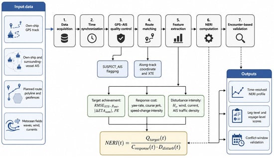
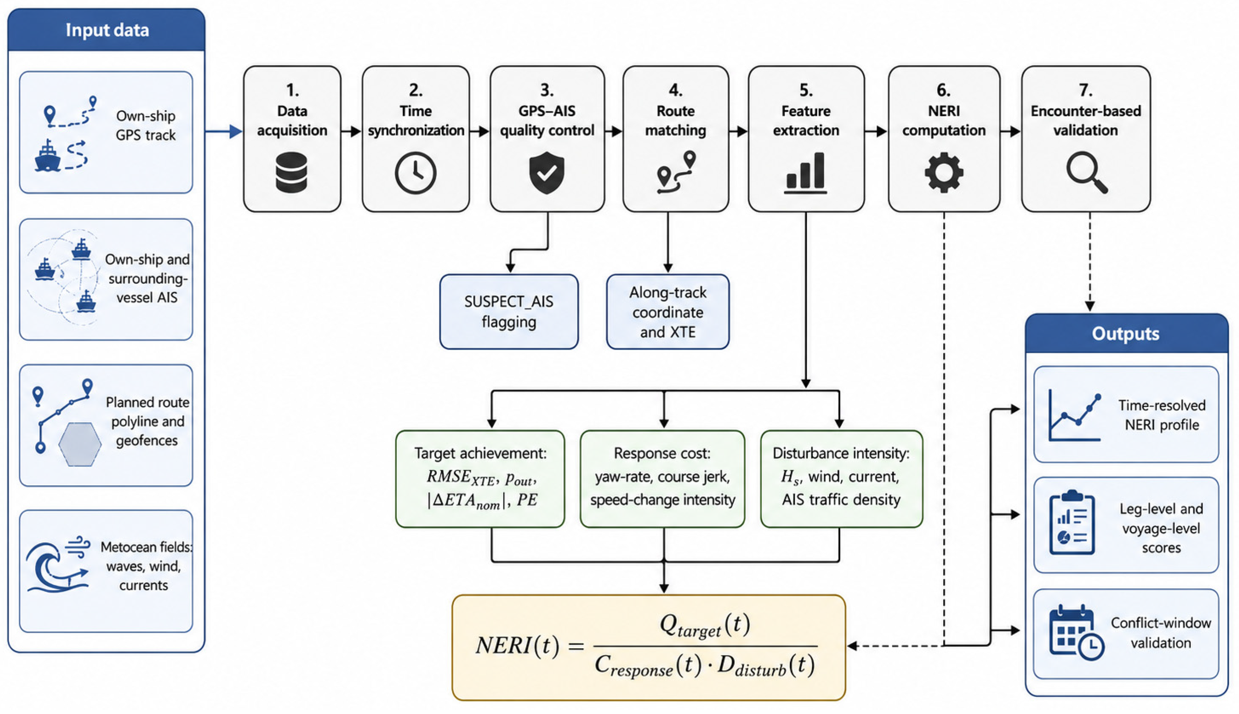
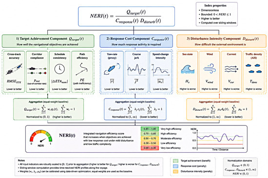
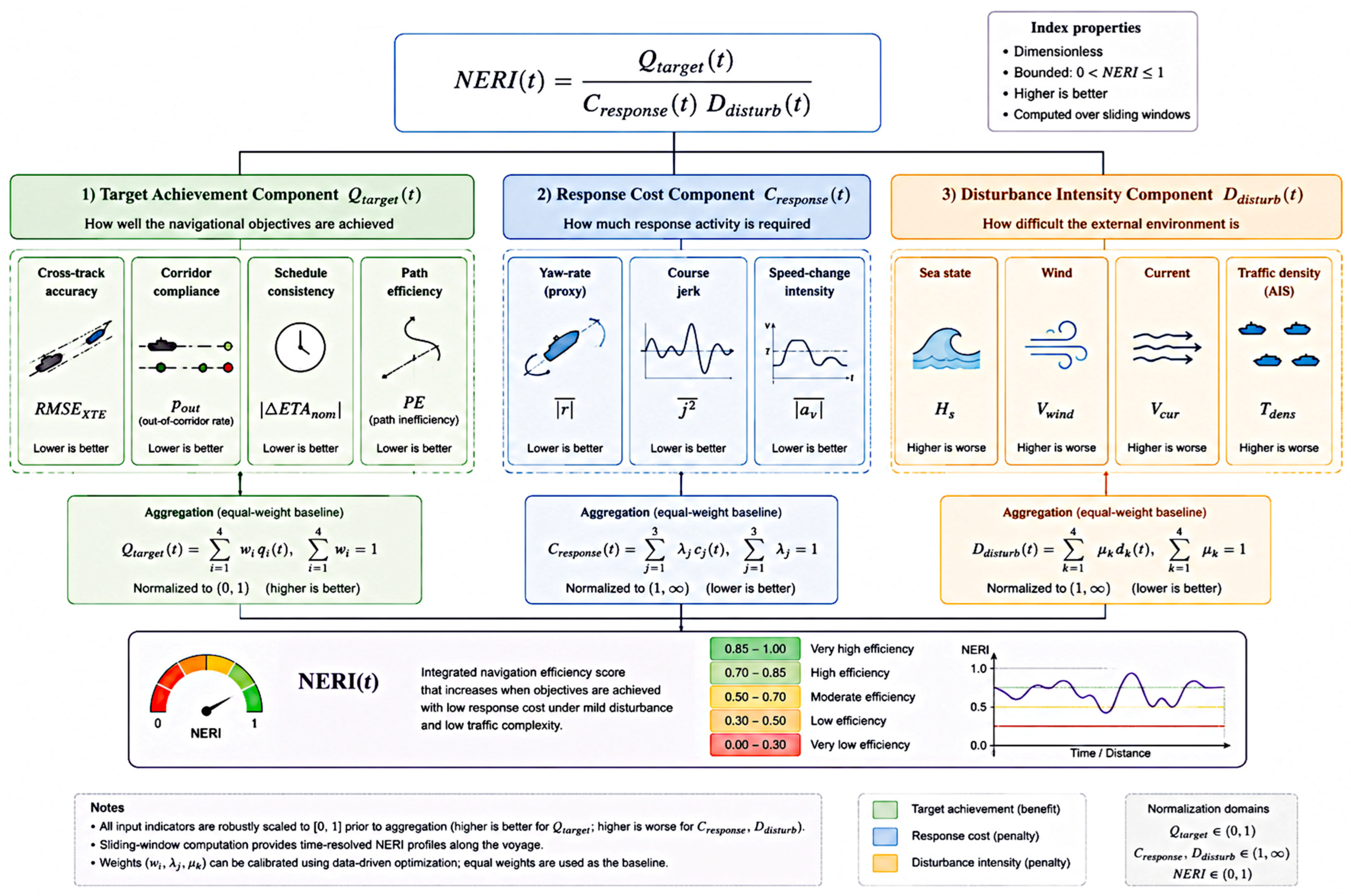
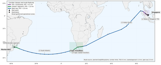
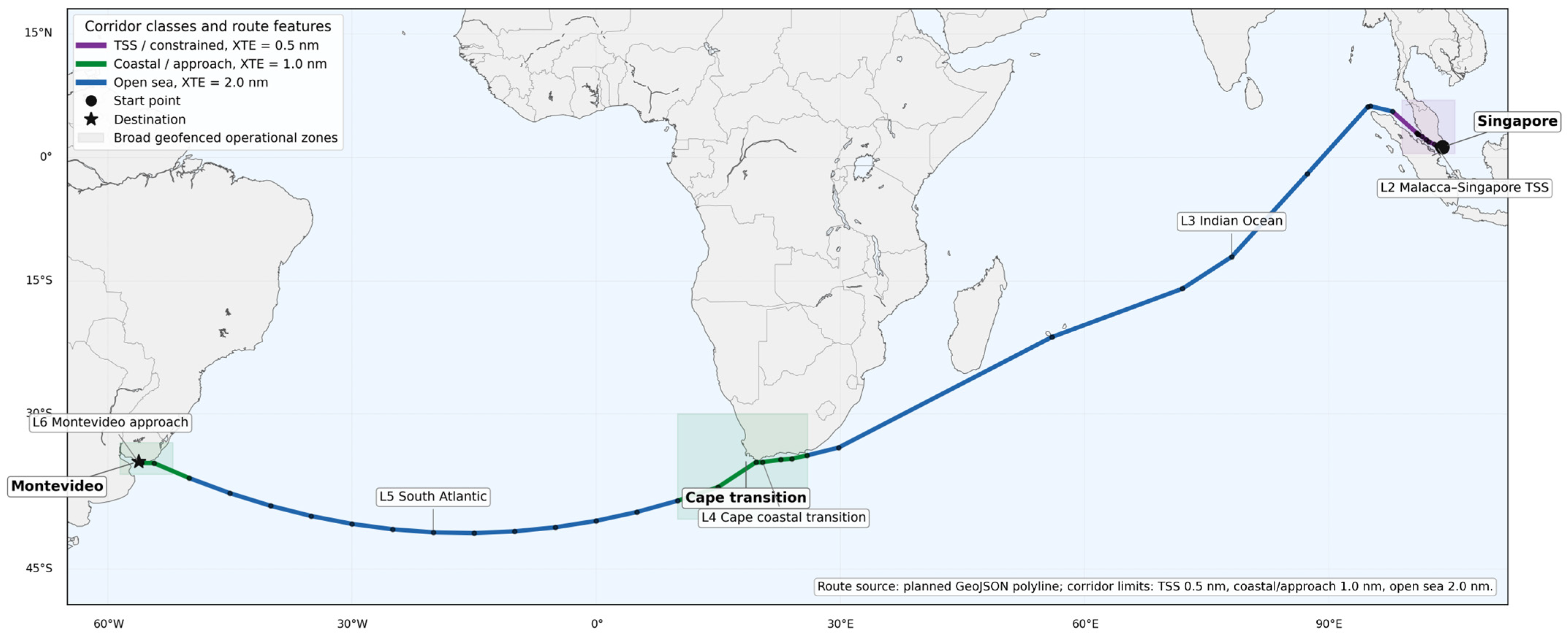
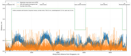
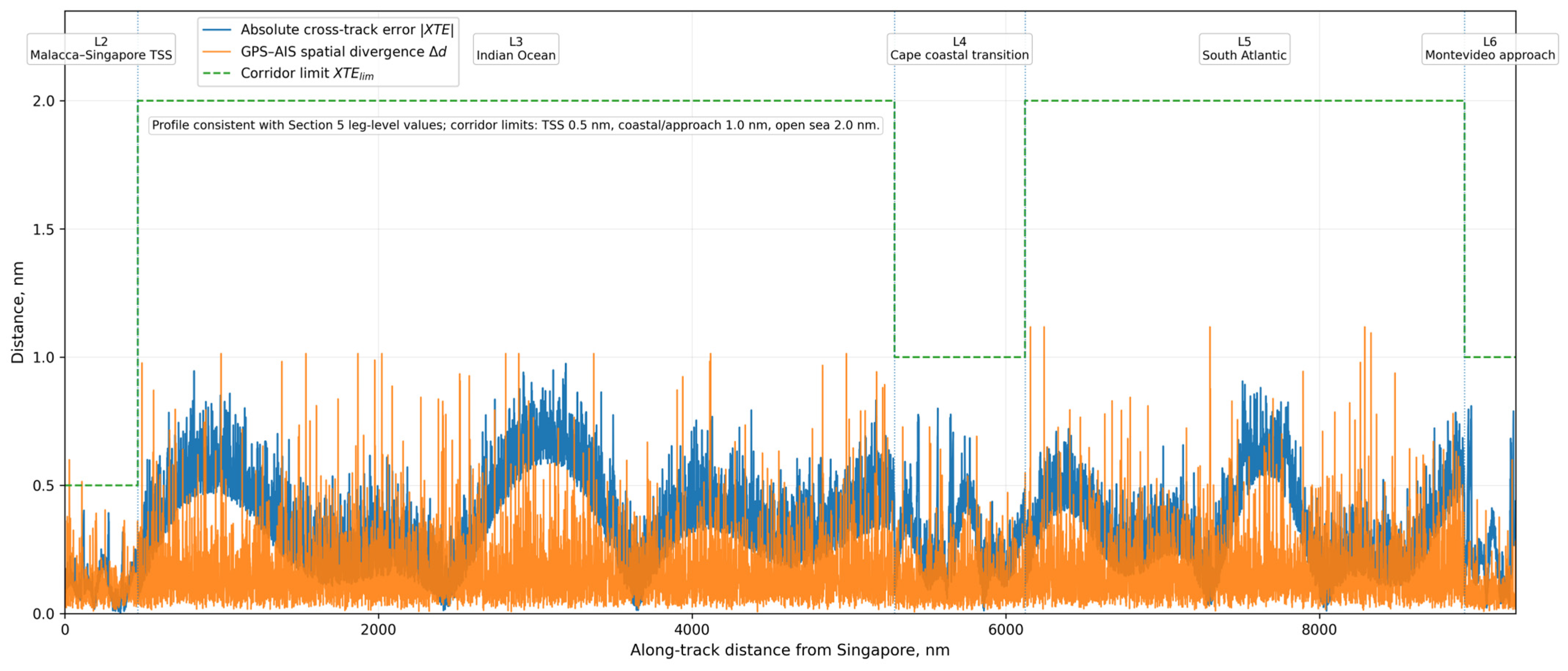
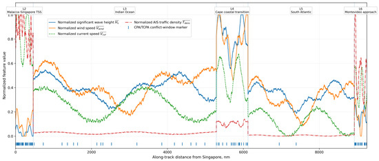
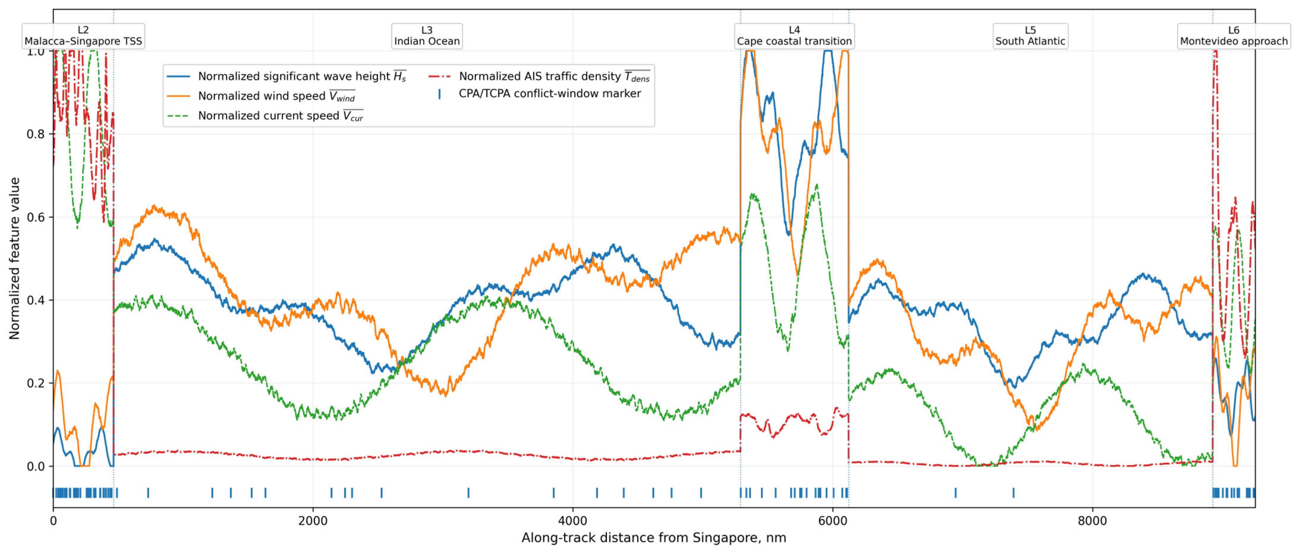
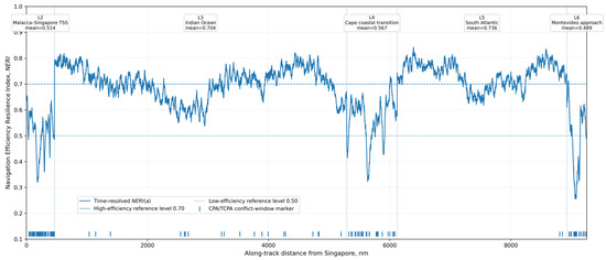
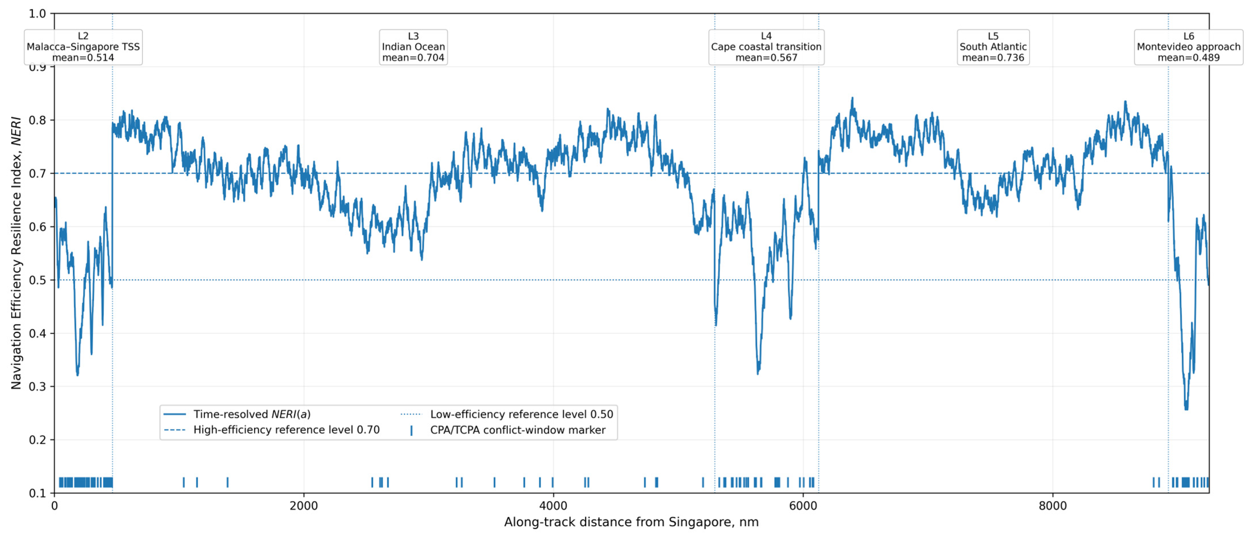
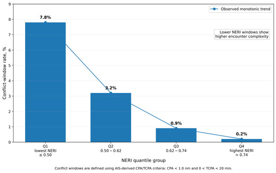
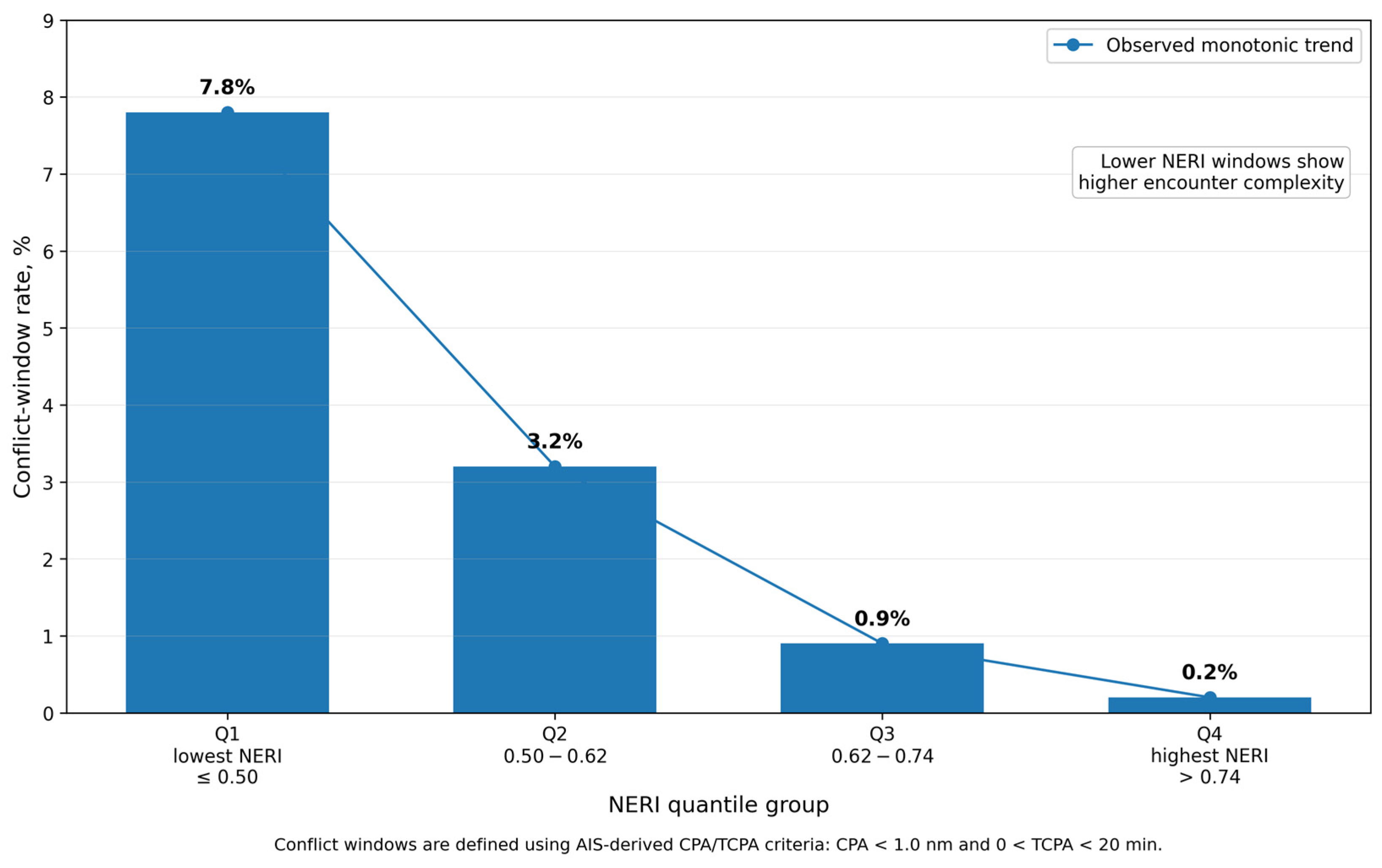
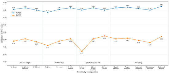
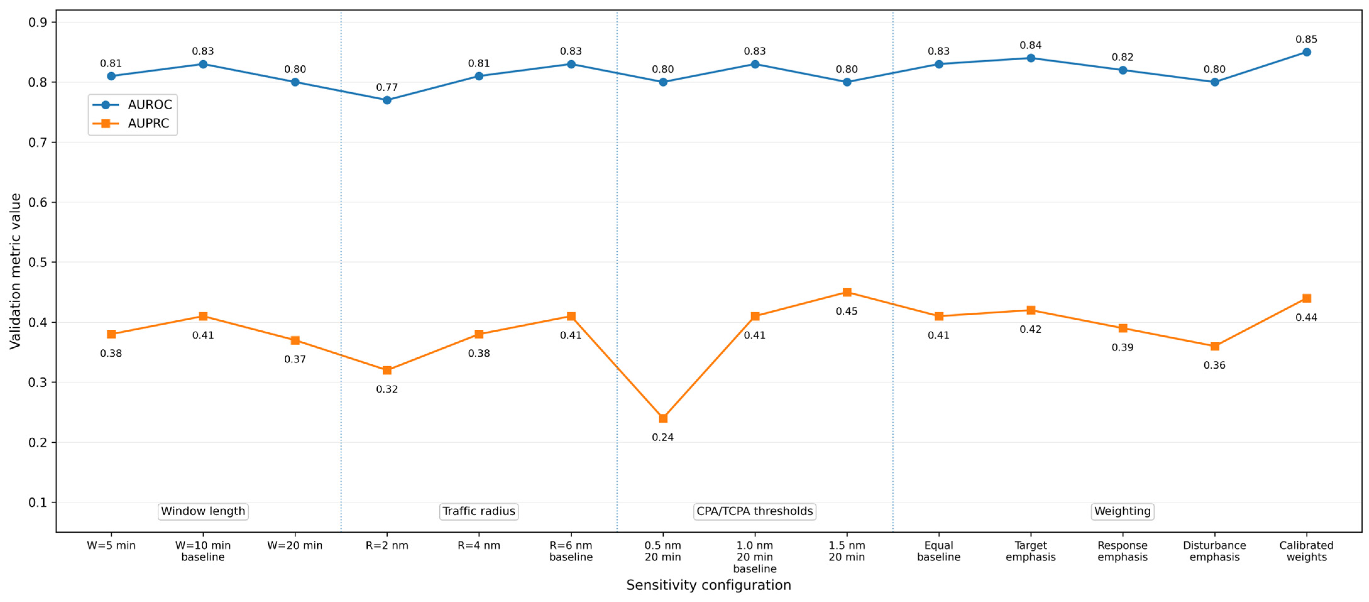

Disclaimer/Publisher’s Note: The statements, opinions and data contained in all publications are solely those of the individual author(s) and contributor(s) and not of MDPI and/or the editor(s). MDPI and/or the editor(s) disclaim responsibility for any injury to people or property resulting from any ideas, methods, instructions or products referred to in the content. |
© 2026 by the authors. Licensee MDPI, Basel, Switzerland. This article is an open access article distributed under the terms and conditions of the Creative Commons Attribution (CC BY) license.