Spatial Heterogeneity Analysis and Machine Learning Prediction of Urban Transport Demand

Abstract

This study investigates the influence of spatial heterogeneity on urban transport demand forecasting. A two-stage framework combining cluster analysis and machine learning was applied to origin-destination trip data generated by a calibrated transport model of a large city. Origin-destination pairs were grouped according to travel conditions using K-Means clustering based on private transport trip length and public transport travel time. The identified clusters were subsequently analyzed with respect to travel costs, modal split, spatial distribution, and transport demand characteristics. Machine learning models were then developed to predict transport demand for public transport, private transport, and walking. Two forecasting strategies were compared: a unified model trained on the entire dataset and cluster-specific models trained separately for each identified cluster. The results revealed significant spatial heterogeneity in travel conditions and transport demand structure. Cluster-specific machine-learning models reduced prediction errors for public and private transport demand, while the magnitude of improvement varied across travel modes and evaluation metrics. The findings demonstrate that accounting for spatial heterogeneity influences transport demand prediction performance, with the greatest improvements observed for public and private transport demand, whereas the effect was less pronounced for walking demand.

1. Introduction

The quality of passenger transport services is an important factor affecting the travel behavior of transport system users [1]. Studies [2,3] show that travel mode choice by urban transport system users depends on a combination of travel costs, socioeconomic factors, and spatial heterogeneity within large cities.

The most important factors determining people’s choice of public transport for urban travel are travel time and trip length. In many large cities, the concept of public transport priority is implemented to ensure the quality of transport services for the population. Priority measures for public transport increase travel speeds on routes and reduce the time costs for public transport users. However, such measures, if implemented without linkage with a set of other measures within an integrated urban transport policy, can increase delays for private transport users, and the overall effect will be insignificant [4].

Due to constraints in road network development in most large cities, existing delays at signalized intersections and on public transport route networks, implementing measures to manage the transport demand structure (modal share by transport mode and travel means) requires significant investment in constructing new or reconstructing existing road and transport infrastructure [5]. When implementing transport policy in a large city, big data analysis is necessary to find optimal solutions. To assess the effectiveness and economic feasibility of measures aimed at improving the urban transport system, modeling traffic and passenger flows is required [6].

After the transport model is created, new calculated data appear, generating big data on the operation of the transport complex based on simulation modeling. One function of a transport macro-model is to store aggregated and processed data on the operation of the transport complex, which are used for validation, calibration, and adequacy assessment of the model. In study [7], the authors note that the city macro-model in the PTV VISUM software is used not only for simulation modeling but also contains a fairly large array of information about various urban objects (transport, road, infrastructure, socio-economic) and is, in essence, a database.

For predictive transport models of a city, artificial neural networks or data mining can be applied. Study [8] shows examples of using neural network technologies to reduce costs for traffic flow monitoring and subsequent forecasting of harmful atmospheric emissions. The authors note that the development of an information environment based on the cloud computing model is promising.

Improving the quality of traffic flow forecasting is currently possible using the advantages of artificial intelligence, which is developing rapidly and being applied in various economic sectors [9]. Machine learning (ML) methods are increasingly used to model travel mode choice and travel behavior. Studies show that advanced ML models can effectively capture nonlinear relationships between transport system characteristics and user decisions, often outperforming traditional approaches [10,11]. Recent research has also highlighted the importance of ML models that not only improve prediction accuracy but also identify the relative importance of factors influencing mode choice behavior [12].

Study [13] applies ML and artificial neural networks to analyze simulation modeling results when studying the mobility structure of the population, taking into account the spatial distribution of residential and work locations, using the example of a large city. All city districts are divided into 9 clusters, in which the shares of trips by private and public transport differ significantly, depending on the average trip distance for work and education purposes. Studies of urban mobility based on big data and ML have shown that urban mobility models exhibit substantial spatial and temporal heterogeneity, which should be considered when analyzing multimodal transport systems and forecasting transport demand [14].

Study [15] assesses gradient-boosting models for predicting travel mode choice using household survey data and demonstrates that travel behavior depends on complex interactions among travel time, distance, and socioeconomic characteristics. The results highlight the importance of accounting for heterogeneity in transport demand and support the use of ML techniques for identifying distinct groups of travel behavior and improving forecasting accuracy. This supports the need to differentiate transport system problems in space and time, establish regularities for groups within the system, and formulate measures for the development of individual subsystems.

Accurate forecasting of transport demand (trip matrices) remains one of the key challenges in transport modeling. Recent studies have proposed ML approaches that account for heterogeneous direct and transfer trips in public transport networks, significantly improving matrix prediction accuracy [16]. Deep learning methods combined with intelligent transportation systems data have also shown great potential for dynamic matrix estimation and real-time transport demand assessment [17]. Feature engineering and integrating multiple transport system variables have been shown to significantly improve matrix estimation accuracy in large transport networks [18].

Recent studies increasingly combine simulation modeling, data analytics, and digital-twin technologies to support decision-making in complex transport and production systems. Simulation environments allow researchers to evaluate the effects of infrastructure and operational changes under different scenarios before their implementation in practice. Studies [19,20] demonstrated the effectiveness of simulation-based approaches for optimizing technological transport systems using the AnyLogic environment, highlighting the ability of simulation models to support operational and strategic planning. Similarly, digital-twin concepts have been successfully applied in industrial and transport-related applications, enabling continuous monitoring, analysis, and optimization of system performance under dynamic conditions.

The growing availability of transport data has also stimulated the development of intelligent decision-support systems that combine mathematical models, simulation tools, and ML techniques. Such systems can improve planning quality, increase operational efficiency, and support infrastructure management under uncertainty. In study [21], the authors demonstrated that integrating analytical models into decision-support frameworks allows managers to evaluate alternative strategies and improve operational performance in transport-related service systems. These developments indicate that the integration of simulation models, digital twins, and data-driven methods represents a promising direction for the evolution of urban transport planning tools.

Previous studies have shown that travel time, trip distance, and socioeconomic characteristics influence travel behavior and mode choice. However, the relationship between travel costs and transport demand is often assumed to be spatially homogeneous across the study area, despite substantial differences in transport infrastructure, accessibility, and urban structure. Previous research has also successfully applied ML methods to predict OD trip matrices, but limited attention has been paid to the spatial differentiation of travel behavior. Consequently, it remains unclear whether accounting for spatial heterogeneity in travel costs improves ML-based transport demand prediction, and whether such improvements depend on travel mode or travel conditions.

The aim of this study is to evaluate how accounting for spatial heterogeneity influences mode-specific transport demand prediction performance. This study hypothesizes that accounting for spatial heterogeneity in travel costs can improve transport demand prediction performance, although the magnitude of improvement may differ across travel modes and travel conditions. To test this hypothesis, a two-stage framework is proposed. First, cluster analysis is applied to identify groups of OD pairs characterized by similar travel conditions. Second, Unified ML and Separate Cluster ML models are developed and compared to evaluate whether accounting for spatial heterogeneity improves prediction performance for different travel modes and travel conditions.

2. Materials and Methods

The proposed methodological workflow consisted of five consecutive stages: (1) extraction of travel costs, trip volumes, and socioeconomic data from the calibrated PTV VISUM model; (2) data preprocessing and filtering of anomalous observations; (3) identification of spatially homogeneous OD groups using clustering; (4) development and optimization of Unified ML and Separate Cluster ML models; and (5) validation and comparison of prediction performance using statistical and spatial analyses.

2.1. Data Generation and Preprocessing

In the developed macroscopic model of a large city (Tyumen, Russia), travel costs were generated using PTV VISUM (https://www.ptvgroup.com/en/products/ptv-visum, accessed on 8 July 2026). Within this study, a database was imported from the morning peak macromodel containing the variables summarized in Table 1 together with their descriptive statistics. In the exported PTV VISUM database, travel-cost values exceeding 999 (min or km) represent origin-destination (OD) pairs for which no feasible route exists. These values do not correspond to actual travel costs and were therefore treated as missing observations and excluded from further analysis. In addition, OD pairs for which both predicted public transport demand and predicted private transport demand were below 0.1 trips were removed from the dataset. The threshold of 0.1 trips was introduced as an author-defined preprocessing criterion intended to remove negligible predicted demand, reduce matrix sparsity, and limit the influence of extremely small absolute values on the subsequent clustering and ML analyses. Walking demand was not subjected to this filtering criterion because walking trips generally exhibit substantially lower trip volumes than motorized transport. Applying the same threshold to walking demand would have removed a considerable number of valid walking trips and consequently distorted the observed distribution of walking demand.

Table 1. Variable definitions and descriptive statistics after preprocessing.

Variable	Description (Units)	Role in the Study	Mean	Std	Median	Min	Max
Public transport travel time	Shortest-path travel time between OD pair by public transport (min)	Clustering and ML Feature	50	20	49	4.8	169
Public transport trip length	Shortest-path trip distance between OD pair by public transport (km)	ML Feature	12	6	11	0.3	42
Private transport travel time	Shortest-path travel time between OD pair by private transport (min)	ML Feature	21	9	20	1.1	91
Private transport trip length	Shortest-path trip distance between OD pair by private transport (km)	Clustering and ML Feature	11	6	10	0.3	49
Walking travel time	Shortest-path travel time between OD pair by walking (min)	ML Feature	138	69	131	2	511
Walking trip length	Shortest-path trip distance between OD pair by walking (km)	ML Feature	9	5	9	0.3	35
Population	Populations’ number of origin and destination zones (persons)	ML Feature	1833	2618	674	0	19,177
Employed residents	Employed residents’ number of origin and destination zones (persons)	ML Feature	1008	1430	383	0	10,418
Jobs	Workplaces’ number of origin and destination zones (jobs)	ML Feature	1036	1313	521	0	9213
Service jobs	Service-sector jobs’ number of origin and destination zones (jobs)	ML Feature	526	665	254	0	3872
Students	Students’ number of origin and destination zones (persons)	ML Feature	123	247	32	0	2677
Educational capacity	Educational capacity of origin and destination zones (persons)	ML Feature	122	663	0	0	7968
Trip volume by public transport	Public transport demand (trips)	ML Target	21	13	20	0.2	50
Trip volume by private transport	Private transport demand (trips)	ML Target	33	11	36	1.1	50
Trip volume by walking	Walking demand (trips)	ML Target	5	12	0.3	0.1	69

The original dataset contained 159,600 observations. After removing disconnected OD pairs and observations with invalid travel costs, 11,213 observations were excluded. An additional 1005 OD pairs were excluded because the predicted trip volume for both public transport and private transport was below the selected threshold of 0.1 trips. The final dataset therefore contained 147,382 observations.

$$D=\left\{\left(i,j\right):0<c_{ij}^m<c_{max}, {(y}_{ij}^{PuT}\ge y_{min} and y_{ij}^{PrT}\ge y_{min})\right\},$$

(1)

where D—filtered dataset used in subsequent analysis; ij—origin and destination zones; m—travel mode (public transport, private transport, or walking); $c_{ij}^m$—travel cost for OD pair ij and travel mode m; $c_{max}$—maximum admissible travel cost value (999 min or km, corresponding to the value exported from PTV VISUM for disconnected OD pairs); $y_{ij}^{PuT}$—trip volume for OD pair ij by public transport; $y_{ij}^{PrT}$—trip volume for OD pair ij by private transport; $y_{min}$—minimum trip volume for OD pair ij used to exclude negligible demand (0.1 trips).

2.2. Clustering for Spatial Heterogeneity Identification

The objective of the clustering procedure was to identify groups of OD pairs characterized by similar travel-cost conditions. Pearson correlation analysis was performed to examine relationships among the candidate travel-cost variables, and the complete correlation matrix is presented in Appendix A. Following the recommendation of Hair et al. [22], variables with pairwise correlations of R ≥ 0.80 were considered to contain substantially redundant information and were not simultaneously included in the clustering procedure. Correlation analysis was used as an initial screening step, whereas the final selection of clustering variables also considered their transport interpretation. Private transport trip length was selected as an indicator of the spatial extent of trips, while public transport travel time was selected as an indicator of public transport service quality. These variables exhibited only moderate mutual correlation (R = 0.77), allowing them to capture complementary aspects of travel conditions while minimizing redundancy. As shown in Appendix A, private transport travel time, public transport trip length, walking travel time, and walking trip length exhibited strong correlations with one or more candidate travel-cost variables and therefore provided limited additional information for clustering. Consequently, these variables were excluded from the clustering procedure. However, the walking-related variables were retained as explanatory variables in the subsequent ML models, where they contributed to the prediction of walking demand. Prior to clustering, the selected variables were standardized using the StandardScaler method, with the mean and standard deviation calculated from the full cleaned dataset. Socioeconomic indicators were not included in the clustering stage because the objective was to identify groups characterized by similar travel cost conditions rather than socioeconomic similarity (Equation (2)).

$$z_{ij}=(L_{ij}^{PrT},T_{ij}^{PuT}), z_{ij, r}^{*}=(z_{ij,r}-{\mu }_r)/{\sigma }_r$$

(2)

where $L_{ij}^{PrT}$—private transport trip length between origin zone i and destination zone j, km; $T_{ij}^{PuT}$—public transport travel time between origin zone i and destination zone j, min; $z_{ij, r}$—value of feature r in vector $z_{ij}$; $z_{ij, r}^{*}$—standardized value of feature r; ${\mu }_r$—mean value of feature r, ${\sigma }_r$—standard deviation value of feature r.

To identify spatial heterogeneity in trip groups with similar travel conditions, several clustering algorithms were evaluated, including K-Means, MiniBatch K-Means, Gaussian Mixture Models, Agglomerative Clustering, and DBSCAN. These algorithms were selected because they represent different clustering assumptions: centroid-based partitioning, scalable centroid-based clustering, probabilistic clustering, hierarchical clustering, and density-based clustering.

For centroid-based and probabilistic methods, the number of clusters was varied from 3 to 10. K-Means and MiniBatch K-Means were initialized with n_init = 20. MiniBatch K-Means used batch_size = 4096. Gaussian Mixture Models used full covariance matrices. Agglomerative clustering used Ward linkage. For DBSCAN, the neighborhood radius (eps) was determined using the k-distance graph and the maximum-distance-from-line (elbow) criterion. The resulting optimal value was 0.085, while min_samples was fixed at 20.

Clustering quality was evaluated using the Silhouette Score, which measures the balance between within-cluster cohesion and between-cluster separation, and the Davies–Bouldin Index, which evaluates the ratio of within-cluster dispersion to between-cluster separation. Both metrics were calculated using their standard implementations in the scikit-learn library (Equation (3)). The final clustering solution was selected by jointly considering internal validation metrics and the interpretability of the resulting OD groups.

$$s\left(i\right)={\displaystyle \frac{b\left(i\right)-a\left(i\right)}{\mathrm{m}\mathrm{a}\mathrm{x}\{a\left(i\right), b(i\left)\right\}}}, DBI={\displaystyle \frac{1}{K}}{\displaystyle \sum _{k=1}^K}\underset{l\ne k}{\max }\left({\displaystyle \frac{{\sigma }_k+{\sigma }_l}{d(c_k,c_l)}}\right)$$

(3)

where a(i)—mean distance between observation i and all other observations in the same cluster (within-cluster cohesion); b(i)—mean distance between observation i and all observations in the nearest neighboring cluster (nearest-cluster separation); σ_k—mean distance of all observations in cluster k to their cluster centroid (within-cluster dispersion); d(c_k, c_l)—distance between the centroids of clusters k and l (between-cluster separation); K—total number of clusters.

For spatial validation, the cluster assignments obtained for individual OD pairs were aggregated to the origin-zone level. For each origin zone, a zonal dominance index was calculated as the proportion of the total trip volume assigned to the dominant cluster. Using a Queen’s contiguity spatial weights matrix, Global Moran’s I was then calculated for this continuous variable rather than for numerical cluster labels to evaluate whether zones with similar degrees of cluster dominance were spatially clustered across the study area (Equation (4)).

$$\begin{gathered} D_i=\underset{k}{\mathrm{m}\mathrm{a}\mathrm{x}}\left({\displaystyle \frac{V_{ik}}{{\displaystyle {\sum }_{k=1}^K}{V}_{ik}}}\right), I={\displaystyle \frac{n}{W}}{\displaystyle \frac{\sum _i\sum _j{w}_{ij}\left(D_i-\overline{D}\right)\left(D_j-\overline{D}\right)}{\sum _i{\left(D_i-\overline{D}\right)}^2}}, \\ w_{ij}=\left\{\begin{array}{c}1, if origin zones i and j share a common boundary or vertex\\ 0, otherwise \end{array}\right. \end{gathered}$$

(4)

where D_i—zonal dominance index for origin zone i, defined as the largest proportion of total trip volume assigned to a single cluster; V_ik—total trip volume originating from zone i and assigned to cluster k; K—total number of clusters; I—Global Moran’s I statistic; W—sum of all spatial weights; w_ij—spatial weight between origin zones i and j; $\overline{D}$—mean zonal dominance index over all origin zones.

To verify that the identified clusters differed in transport demand characteristics beyond the variables used for clustering, additional Kruskal–Wallis H tests (Equation (5)) were performed using mode-specific trip volumes that were not included in the clustering procedure. The corresponding effect sizes (η²) were calculated according to Equation (5) to quantify the practical magnitude of the observed inter-cluster differences.

$$H={\displaystyle \frac{12}{N(N+1)}}{\displaystyle \sum _{i=1}^k}{\displaystyle \frac{R_i^2}{n_i}}-3(N+1), { \eta }^2={\displaystyle \frac{H-k+1}{N-k}}$$

(5)

where H—Kruskal–Wallis test statistic; N—total number of observations included in the statistical test; k—number of compared clusters; R_i—sum of ranks for observations belonging to cluster i; n_i—number of observations in cluster i; η²—effect size estimating the proportion of variability explained by the differences between clusters.

The resulting clusters were subsequently used to analyze spatial heterogeneity in transport demand and to evaluate their contribution to ML-based transport demand forecasting.

2.3. ML Models for Transport Demand Forecasting

The ML task was to forecast transport demand and to evaluate the impact of accounting for spatial heterogeneity on prediction accuracy. The analysis was performed separately for public transport, private transport, and walking.

The target variables were trip volumes between OD pairs for public transport, private transport, and walking. The X variables included travel costs (time and distance for different travel modes) and zonal socioeconomic indicators.

To evaluate the contribution of spatial heterogeneity information, two ML forecasting strategies were compared. The first strategy (Unified ML) used unified ML models trained on the entire dataset without clustering results. The second strategy (Separate Cluster ML) used separate ML models estimated independently for each identified cluster. Comparison of these two strategies enabled assessment of the impact of spatial heterogeneity on prediction accuracy (Equation (6)). In the Separate Cluster ML strategy, the cluster label is used only to partition the dataset into homogeneous subsets before model training and is not included as an explicit predictor in the ML models. The unified ML models were considered the baseline forecasting approach, while the clustered ML models represented the proposed framework.

$$\begin{gathered} {\widehat{y}}_{ij}^m=\left\{\begin{array}{cc}{f}_m\left(x_{ij}\right), & Unified ML\hfill \\ f_{m,k}\left(x_{ij}\right), & Separate Cluster ML\hfill \end{array}\right. , \\ {x}_{ij}=(L_{ij}^{PrT},L_{ij}^{PuT},L_{ij}^W,T_{ij}^{PrT},T_{ij}^{PuT},T_{ij}^W,P_i,P_j,{Em}_i,{Em}_j,J_i,J_j,{SJ}_i,{SJ}_j,S_i,S_j,{Ed}_i,{Ed}_j) \end{gathered}$$

(6)

where ${\widehat{y}}_{ij}^m$—predicted trip volume between origin zone i and destination zone j for travel mode m, trips; ij—origin and destination zones; m—travel mode (public transport, private transport, or walking); $f_m\left(x_{ij}\right)$—ML model trained using the complete dataset (Unified ML strategy) separately for travel mode m; $f_{m,k}\left(x_{ij}\right)$—ML model trained separately for travel mode m and cluster k (Separate Cluster ML strategy); k—cluster identified during the clustering stage;$x_{ij}$—feature vector describing the OD pair ij; $L_{ij}^{PrT}$—private transport trip length, km; $L_{ij}^{PuT}$—public transport trip length, km; $L_{ij}^W$—walking trip length, km; $T_{ij}^{PrT}$—private transport travel time, min; $T_{ij}^{PuT}$—public transport travel time, min; $T_{ij}^W$ walking travel time, min; P_i, P_j—population of the origin i and destination j zone, persons; Em_i, Em_j—employed residents of the origin i and destination j zone, persons; J_i, J_j –jobs of the origin i and destination j zone, jobs; SJ_i, SJ_j—service jobs of the origin i and destination j zone, jobs; S_i, S_j—students of the origin i and destination j zone, persons; Ed_i, Ed_j—educational capacity of the origin i and destination j zone, persons.

Both the Unified ML and Separate Cluster ML strategies evaluated the same supervised learning algorithms, including Decision Tree Regressor, Random Forest Regressor, Gradient Boosting Regressor, and HistGradientBoosting Regressor. All candidate hyperparameter configurations were evaluated on the training data, and the combination yielding the best cross-validation score was selected. The optimized model was then retrained using the complete training dataset and evaluated on the independent test dataset. The investigated hyperparameter search ranges are provided in Appendix B.

For the ML models, additional feature scaling was not performed, since the algorithms used are not sensitive to differences in variable scale. The dataset was randomly split into training and test sets with a 50/50 ratio. Model selection was performed independently for each travel mode and/or cluster. The final model configuration was selected based on the minimum mean absolute percentage error (MAPE) value obtained during the cross-validation procedure. Model performance was evaluated on an independent test dataset using four complementary metrics: MAPE, mean absolute error (MAE), root mean squared error (RMSE), and the coefficient of determination R². For the Separate Cluster ML strategy, independent models were trained for each cluster. After prediction, the observed and predicted values from all cluster-specific test sets were concatenated into a single pooled dataset for each travel mode. The Combined performance metrics were then calculated from this pooled dataset rather than by averaging the cluster-specific metric values, thereby enabling direct comparison with the Unified ML strategy.

3. Results

3.1. Clustering for Spatial Heterogeneity Identification

The clustering analysis revealed distinct groups of OD pairs with similar travel conditions, supporting the presence of spatial heterogeneity in the study area. Table 2 summarizes the performance of the evaluated clustering algorithms and the characteristics of the selected clustering solution.

Table 2. Comparison of clustering algorithms’ performance.

Method	Hyperparameters	Number of Clusters	Noise Points	Silhouette Score	Davies–Bouldin Index
K-Means	n_init = 20	3	0	0.49	0.75
		4	0	0.48	0.8
		5	0	0.47	0.81
MiniBatch K-Means	batch_size = 4096; n_init = 20	3	0	0.45	0.78
		4	0	0.44	0.82
		5	0	0.43	0.83
Gaussian Mixture Model	covariance = full	3	0	0.43	0.82
		4	0	0.39	0.86
		5	0	0.37	0.93
Agglomerative Clustering	linkage = ward	3	0	0.38	0.85
		4	0	0.39	0.81
		5	0	0.38	0.9
DBSCAN	eps = 0.085; min_samples = 20	10	2140	0.09	0.58

The K-Means and MiniBatch K-Means algorithms provided the most balanced combination of cluster compactness and separation quality. DBSCAN showed the lowest Davies-Bouldin Index; however, it identified ten clusters and a large number of noise points, and the corresponding Silhouette Score was substantially lower than for centroid-based methods. Therefore, the K-Means algorithm was selected as the primary clustering method. Although the highest Silhouette Score was obtained for three clusters, the resulting segmentation was coarse and combined OD pairs characterized by substantially different travel conditions. Five clusters provided a compromise between clustering quality and interpretability.

The cluster analysis identified five distinct groups of OD pairs (Table 3). Cluster 3 is the largest group (31% of OD pairs) with moderate travel conditions. Cluster 4, the smallest group (4% of OD pairs), represents long-distance trips with the highest mean travel times (85 min by public transport, 40 min by private transport) and trip lengths (22 km by public transport, 30 km by private transport). The walking mode share varies substantially across clusters, from 0.4% (Cluster 1) to 21.4% (Cluster 2), reflecting differences in short-distance accessibility. The public transport share ranges from 18.8% (Cluster 4) to 40.5% (Cluster 3), indicating varying levels of public transport service quality across clusters.

Table 3. Clusters characteristics.

Cluster Number		1	2	3	4	5
Number of OD pairs		20,067	34,505	45,813	6096	40,901
Share of OD pairs, %		14	23	31	4	28
Mean travel time, min	by public transport	78	26	43	85	59
	by private transport	33	11	18	40	25
Mean trip length, km	by public transport	19	5	9	22	14
	by private transport	18	4	8	30	13
Trip volume	by public transport	41,676	366,456	429,116	8909	198,601
	by private transport	159,247	394,167	611,999	34,422	434,959
	by walking	920	206,536	17,253	219	3082
	total	201,843	967,159	1,058,368	43,550	636,642
Share, %	by public transport	20.7	39	40.5	18.8	30.9
	by private transport	78.9	39.6	57.8	80.7	68.3
	by walking	0.4	21.4	1.7	0.5	0.8

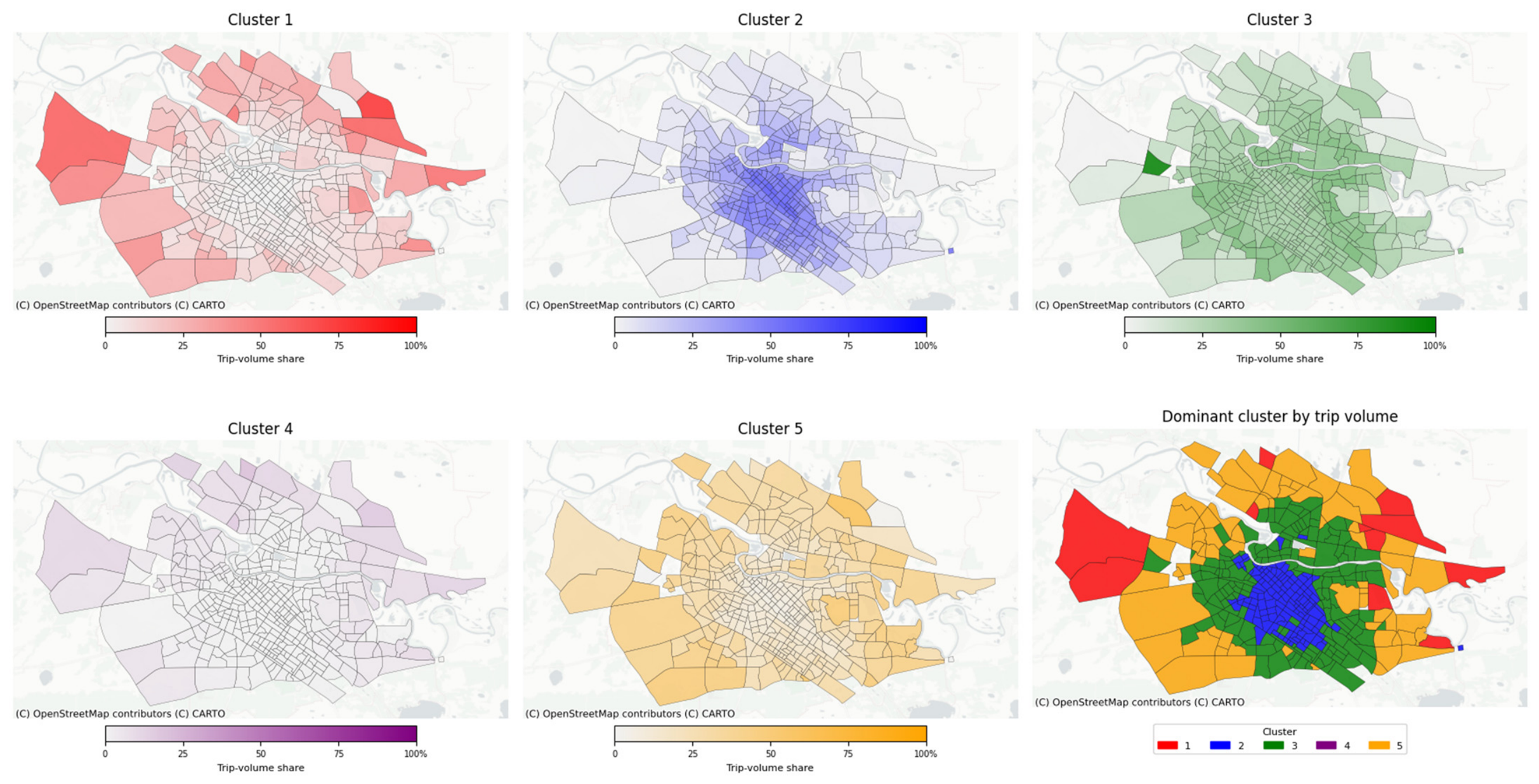
The spatial distribution of the identified clusters is shown in Figure 1. The first five maps illustrate the share of trip volume generated by each zone and assigned to the corresponding cluster. The last map shows the dominant cluster per zone, determined by the maximum trip volume generated by that zone.

Figure 1. Spatial distribution of OD-pair clusters by trip-volume share and dominant cluster per zone.

The results show that clusters are not uniformly distributed across the study area; instead, they form distinct spatial patterns related to differences in accessibility, travel costs, and transport network configuration. Central zones are predominantly associated with Clusters 2 and 3, characterized by shorter trip distances and higher accessibility. Peripheral zones, especially those separated by major barriers (river, railway, bypass road), are more strongly associated with Clusters 4 and 5, characterized by longer travel times and higher travel costs.

The resulting Moran’s I value was 0.313 (p = 0.001), indicating moderate positive spatial autocorrelation. This suggests that zones with similar cluster membership in terms of travel costs are geographically grouped, confirming spatial heterogeneity in travel costs. Although clustering was performed using travel-cost variables rather than geographic coordinates, the resulting clusters exhibit clear spatial concentration patterns across the city. This indicates that differences in travel conditions have a spatial structure and are related to the road network and public transport route network configuration.

The identified clusters exhibit substantial differences in transport demand structure. Clusters with short trips are characterized by a significant walking share, whereas clusters with long-distance trips are associated with higher private transport use. Intermediate clusters show varying transport demand structures, reflecting differences in accessibility and travel conditions across the city.

The Kruskal–Wallis H tests confirmed statistically significant differences between clusters in public transport trip volume (H = 86,611, p < 0.05), private transport trip volume (H = 51,542, p < 0.05), and walking trip volume (H = 121,504, p < 0.05). The corresponding effect sizes (η²) were 0.59, 0.35, and 0.82, respectively, indicating moderate to large practical differences in transport demand characteristics among the identified clusters. These findings demonstrate that the clusters differ not only in travel cost conditions, which formed the basis of the clustering procedure, but also in transport demand characteristics that were not used during cluster formation.

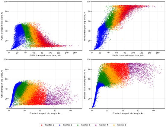
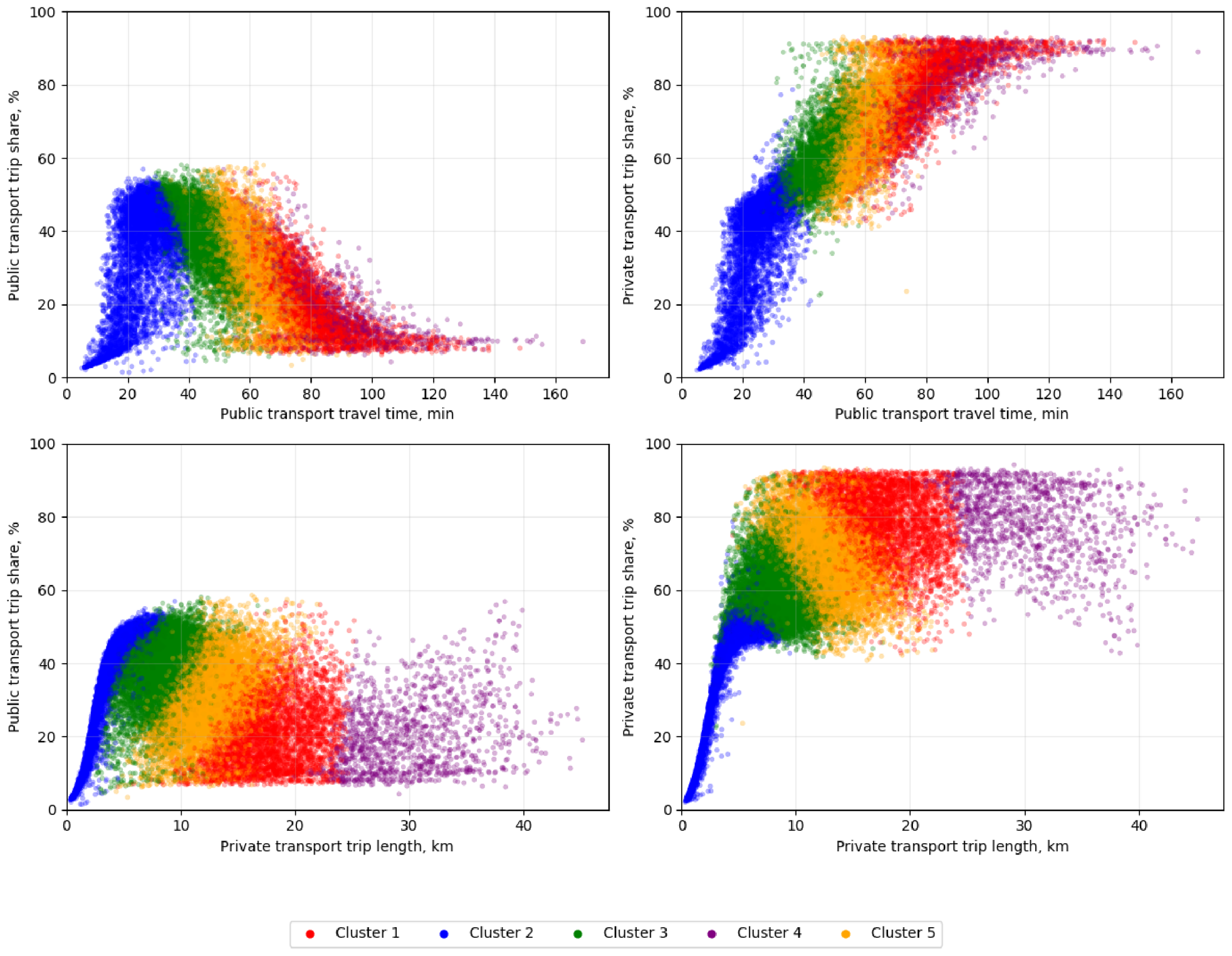
The relationship between costs and mode choice varies by cluster (Figure 2). Clusters are characterized by different combinations of costs and transport demand structure. The change in transport demand structure in response to cost changes may differ across clusters, indicating a potential need to account for spatial heterogeneity when designing and evaluating urban transport system measures.

Figure 2. Effect of travel costs on mode choice across clusters.

Overall, the five clusters differ in travel costs (Table 3 and Figure 2) and spatial location (Figure 1). These results confirm the presence of spatial heterogeneity in transport demand structure and provide a basis for cluster-specific ML forecasting.

3.2. ML Models for Transport Demand Forecasting

Table 4 presents the prediction metrics obtained for the two forecasting strategies. For strategy Unified ML, 3 models were independently trained and evaluated for each travel mode; for Separate Cluster ML, 15 cluster-specific models (5 clusters × 3 travel modes) were trained. The results indicate that the influence of spatial heterogeneity differs across travel modes. Separate Cluster ML reduced absolute prediction errors for public and private transport, whereas improvements for walking mode were not reflected across all evaluation metrics. Comparing Unified ML and Separate Cluster ML (combined—pooled test sample across clusters) shows that the improvement is related to the inclusion of spatial heterogeneity information rather than to the ML algorithms and their parameters themselves.

Table 4. ML model performance by strategy, travel modes, and clusters.

Travel Modes	Models	Strategy or Cluster	MAPE, %	MAE, Trips	RMSE, Trips	R2
Public transport	HistGradientBoostingRegressor: learning_rate = 0.1, max_iter = 200, max_leaf_nodes = 31, min_samples_leaf = 50	Unified ML	14	0.56	0.84	0.96
Private transport			8	0.71	0.98	0.92
Walking			10	0.13	0.42	0.9
Public transport	HistGradientBoostingRegressor: learning_rate = 0.1, max_iter = 200, max_leaf_nodes = 31, min_samples_leaf = 50	1	18	0.31	0.46	0.84
		2	4	0.34	0.58	0.98
		3	10	0.62	0.91	0.88
		4	22	0.24	0.42	0.86
		5	17	0.59	0.82	0.84
		Combined	12	0.48	0.73	0.97
Private transport	HistGradientBoostingRegressor: learning_rate = 0.1, max_iter = 200, max_leaf_nodes = 31, min_samples_leaf = 20	1	12	0.84	1.09	0.87
		2	2	0.17	0.24	0.99
		3	3	0.44	0.59	0.85
		4	6	0.31	0.46	0.97
		5	9	0.8	1.04	0.83
		Combined	6	0.53	0.71	0.95
Walking	HistGradientBoostingRegressor: learning_rate = 0.05, max_iter = 100, max_leaf_nodes = 15 min_samples_leaf = 20	1	6	0.04	0.07	0.16
		2	3	0.08	0.17	0.99
		3	15	0.06	0.19	0.96
		4	0.3	0.01	0.01	0.98
		5	14	0.02	0.21	0.44
		Combined	10	0.04	0.17	0.72

The highest prediction accuracy was achieved using ensemble ML methods. HistGradientBoosting was selected as the most accurate model for all transport demand predictions. Although a separate model was trained for each travel mode and cluster in both strategies, most models used the same hyperparameters determined by GridSearchCV.

The results show that prediction accuracy varies considerably across clusters, reflecting differences in travel conditions and transport demand patterns. The Combined performance metrics (MAPE, MAE, RMSE, and R²) were calculated from the pooled test observations across all clusters rather than as averages of the corresponding cluster-specific metrics. Therefore, they represent the overall prediction performance across all OD pairs for each travel mode. The Combined R² is not a simple average of the cluster-specific R² values, but is computed from the pooled sample, which may result in a value that differs substantially from the individual cluster-specific values. This suggests that clustering primarily reduced absolute prediction errors, whereas the coefficient of determination R² remained more sensitive to the comparatively low variability and smaller absolute trip volumes associated with walking demand.

For public transport demand forecasting, the lowest prediction errors were obtained in Cluster 2, where the selected HistGradientBoosting model achieved a MAPE of 4% and an R² of 0.98. Higher errors were observed in Clusters 1, 4, and 5, which is attributed to greater variability in transport demand structure within these clusters. Nevertheless, all public transport models achieved R² values above 0.8, indicating a high degree of fit between observed and predicted values.

Overall, private transport demand forecasting was more accurate. The HistGradientBoosting model was selected as the most effective for all clusters, with MAPE values ranging from 2% to 12%. The highest coefficients of determination were observed in Cluster 2 (R² = 0.99) and Cluster 4 (R² = 0.97). This indicates that transport demand within these clusters exhibits more stable relationships with travel costs and socioeconomic characteristics.

For walking trips, the HistGradientBoosting models provided accurate predictions. The obtained MAPE values ranged from 0.3% to 15%. Although the coefficients of determination varied considerably across clusters, prediction errors remained relatively small due to the lower absolute trip volumes associated with walking.

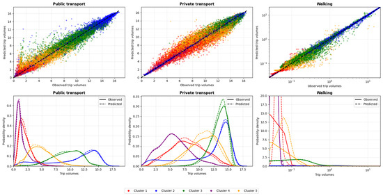
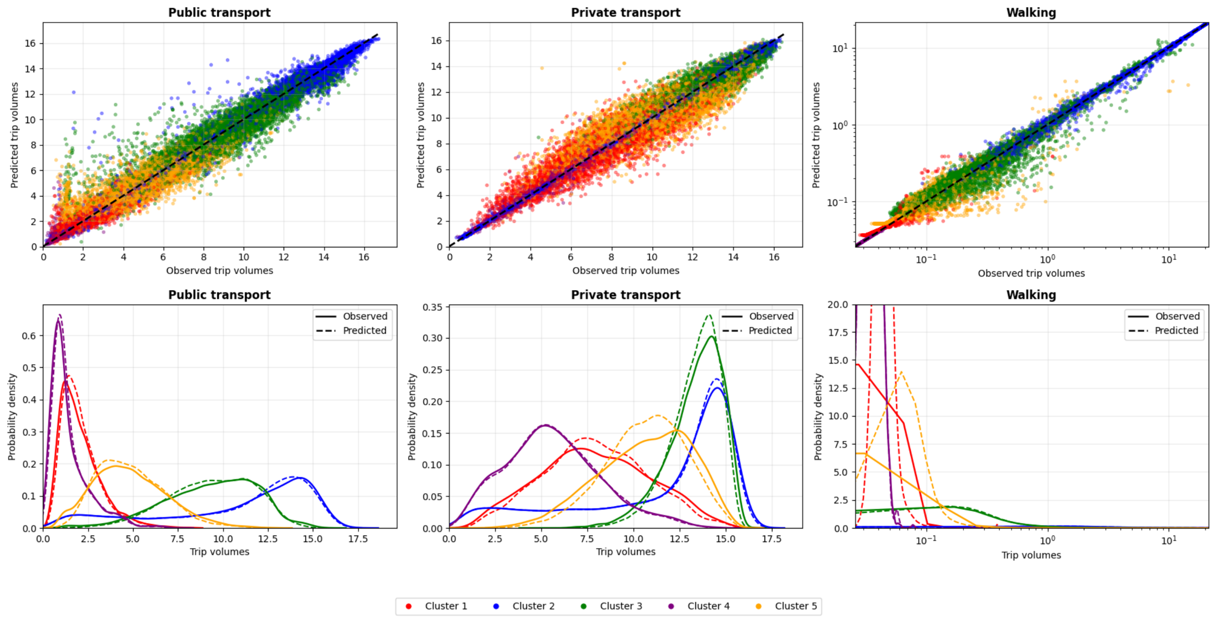
Figure 3 compares the observed and predicted transport demand values for the selected ML models. The plots demonstrate a high level of agreement between predicted and observed values. The density distributions further confirm that the models reproduce the overall transport demand structure within the clusters.

Figure 3. Observed vs. predicted transport demand values by travel modes and clusters.

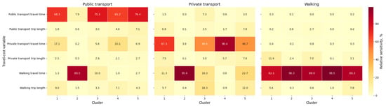
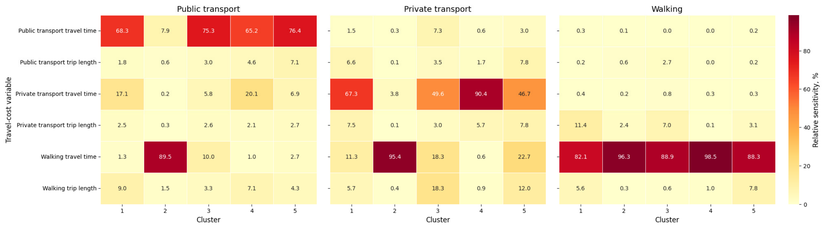
To investigate variable contributions and ML model interpretability, a sensitivity analysis was performed for each cluster. Relative sensitivity values were calculated for each cluster and travel mode and normalized within each model. Figure 4 presents the relative importance of travel-cost variables for predicting demand by different travel modes.

Figure 4. Relative sensitivity of travel cost variables across clusters and travel modes.

The sensitivity analysis revealed differences in the relative importance of travel-cost variables across clusters. Public transport demand in Clusters 1, 3, 4, and 5 was primarily associated with in-vehicle time, whereas in Cluster 2, walking access/egress time became the dominant factor. A similar pattern was observed for private transport demand forecasting: the importance of time-related variables varied from cluster to cluster. In contrast, walking demand was consistently dominated by walking time, indicating a more homogeneous behavioral structure. These findings suggest that spatial heterogeneity is more pronounced for motorized trips than for walking trips.

The obtained results indicate that spatial heterogeneity affects the transport demand structure. Its contribution to ML prediction performance depends on travel mode, with the largest improvements observed for public and private transport demand.

4. Discussion

Transport demand in a large city exhibits pronounced spatial heterogeneity related to differences in travel costs. The spatial distribution of clusters indicates that travel costs are closely linked to the city’s zoning pattern. Central zones are predominantly associated with clusters characterized by shorter trips and higher accessibility, whereas peripheral zones separated by major transport barriers are associated with clusters with higher travel costs. These findings suggest that transport system improvements may have substantially different effects across different parts of the city. The identified clusters differ not only in travel costs but also in transport demand structure. Statistical testing indicated that these differences are substantial and represent meaningful patterns.

The ML results indicate that the influence of spatial heterogeneity depends on travel mode. Comparing the Unified ML and Separate Cluster ML strategies showed that separate Cluster ML generally reduced MAE, RMSE, and MAPE compared with Unified ML, although improvements were not consistent across all evaluation metrics. In particular, the coefficient of determination remained lower for some cluster-specific walking models. These results indicate that accounting for spatial heterogeneity mainly improves absolute prediction errors rather than uniformly improving every performance metric.

The analysis was conducted using data generated by a calibrated transport model for a single large city. Therefore, the identified clusters depend on local transport network characteristics, and the models reproduce patterns represented in the calibrated transport model rather than observed travel behavior in the city. Consequently, the generalizability of the proposed framework to other urban contexts requires further validation. Future research should focus on testing the proposed framework on real-world data, in other cities, incorporating additional cost indicators, and assessing the temporal stability of the identified clusters.

Overall, the results indicate that spatial heterogeneity is an important characteristic of transport demand. Combining cluster analysis with ML methods provides a framework for investigating the influence of spatial heterogeneity on transport demand prediction and may improve forecasting performance, particularly for motorized travel modes.

References

- Wang, J.; Li, J.; Zhang, Y.; Long, X. Research on Influencing Factors of Transportation Mode Selection Behavior in Urban Agglomerations Considering Travel Preferences. J. Beijing Jiaotong Univ. 2024, 48, 22–31. [Google Scholar] [CrossRef]
- Acheampong, R.A.; Cugurullo, F.; Gueriau, M.; Dusparic, I. Can Autonomous Vehicles Enable Sustainable Mobility in Future Cities? Insights and Policy Challenges from User Preferences over Different Urban Transport Options. Transp. Res. Part C Emerg. Technol. 2021, 122, 102869. [Google Scholar] [CrossRef] [Scilit]
- Herath, D.; Dharmarathna, W.R.S.S.; Wickramasinghe, V.; Edirisinghe, J. Travel Behaviour Analysis and Exploration of Mode Choice Variability of Short-Distance Travellers. Eng. J. Inst. Eng. Sri Lanka 2023, 56, 51–62. [Google Scholar] [CrossRef] [Scilit]
- Pistsov, A.; Zakharov, D. Analysis of Methods of Providing Public Transport Priority in Cities. WIT Trans. Built Environ. 2021, 204, 293–302. [Google Scholar] [CrossRef] [Scilit]
- Morozov, V.; Shepelev, V.; Kostyrchenko, V. Modeling the Operation of Signal-Controlled Intersections with Different Lane Occupancy. Mathematics 2022, 10, 4829. [Google Scholar] [CrossRef] [Scilit]
- Morozov, V.; Petrov, A.I.; Shepelev, V.; Balfaqih, M. Ideology of Urban Road Transport Chaos and Accident Risk Management for Sustainable Transport Systems. Sustainability 2024, 16, 2596. [Google Scholar] [CrossRef] [Scilit]
- Atanasova, V.; Stojanoska, M. Study of Steps in the VISUM Software for Creating a Macroscopic Model for Public Transport, for Example for the City of Prilep. Ger. Int. J. Mod. Sci. 2023, 68, 51–54. [Google Scholar] [CrossRef]
- Mekouar, Y.; Saleh, I.; Karim, M. GreenNav: Spatiotemporal Prediction of CO2 Emissions in Paris Road Traffic Using a Hybrid CNN-LSTM Model. Network 2025, 5, 2. [Google Scholar] [CrossRef] [Scilit]
- Yusuf, O.; Rasheed, A.; Lindseth, F. Leveraging Big Data and AI for Sustainable Urban Mobility Solutions. Urban Sci. 2025, 9, 301. [Google Scholar] [CrossRef] [Scilit]
- Martin-Baos, J.Á.; López-Gómez, J.A.; Rodriguez-Benitez, L.; Hillel, T.; García-Ródenas, R. A Prediction and Behavioural Analysis of Machine Learning Methods for Modelling Travel Mode Choice. Transp. Res. Part C Emerg. Technol. 2023, 156, 104318. [Google Scholar] [CrossRef] [Scilit]
- Wang, F.; Ross, C.L. Machine Learning Travel Mode Choices: Comparing the Performance of an Extreme Gradient Boosting Model with a Multinomial Logit Model. Transp. Res. Rec. 2018, 2672, 35–45. [Google Scholar] [CrossRef] [Scilit]
- Dahmen, V.; Weikl, S.; Bogenberger, K. Interpretable Machine Learning for Mode Choice Modeling on Tracking-Based Revealed Preference Data. Transp. Res. Rec. 2024, 2678, 2075–2091. [Google Scholar] [CrossRef] [Scilit]
- Chainikov, D.; Zakharov, D.; Kozin, E.; Pistsov, A. Studying Spatial Unevenness of Transport Demand in Cities Using Machine Learning Methods. Appl. Sci. 2024, 14, 3220. [Google Scholar] [CrossRef] [Scilit]
- Kiros, A.; Ribakov, Y.; Klein, I.; Cohen, A. GeoAI and Multimodal Geospatial Data Fusion for Inclusive Urban Mobility: Methods, Applications, and Future Directions. Urban Sci. 2026, 10, 193. [Google Scholar] [CrossRef] [Scilit]
- Pineda-Jaramillo, J.; Arbelaez-Arenas, O. Assessing the Performance of Gradient-Boosting Models for Predicting the Travel Mode Choice Using Household Survey Data. J. Urban Plan. Dev. 2022, 148, 04022007. [Google Scholar] [CrossRef] [Scilit]
- Tang, T.; Mao, J.; Liu, R.; Liu, Z.; Wang, Y.; Huang, D. Origin-Destination Matrix Prediction in Public Transport Networks: Incorporating Heterogeneous Direct and Transfer Trips. IEEE Trans. Intell. Transp. Syst. 2024, 25, 19889–19903. [Google Scholar] [CrossRef] [Scilit]
- Afandizadeh Zargari, S.; Memarnejad, A.; Mirzahossein, H. Hourly Origin–Destination Matrix Estimation Using Intelligent Transportation Systems Data and Deep Learning. Sensors 2021, 21, 7080. [Google Scholar] [CrossRef] [Scilit] [PubMed]
- Sharma, S. Enhancing Dynamic Origin-Destination (OD) Matrix Estimation for Large Networks Through Feature Engineering: A Comprehensive Framework. Ph.D. Thesis, Queensland University of Technology, Brisbane, Australia, 2024. [Google Scholar]
- Bauer, V.I.; Kozin, E.S.; Bazanov, A.V.; Nemkov, M.V.; Mukhortov, A.A. Optimization of Technological Transport Sets Using AnyLogic Simulation Environment. J. Mech. Eng. Res. Dev. 2019, 42, 41–43. [Google Scholar] [CrossRef] [Scilit]
- Kozin, E.S. Decision Support System for the Management of a Vehicle Service Workshop. J. Manag. Technol. 2023, 23, 88–102. [Google Scholar] [CrossRef] [Scilit]
- Kozin, E.S. Operational Management of Production for Car Maintenance and Repair Using Digital Twin Technology. In The Future of Industry; Lecture Notes in Information Systems and Organisation; Springer: Cham, Switzerland, 2024; Volume 70. [Google Scholar] [CrossRef] [Scilit]
- Hair, J.F.; Black, W.C.; Babin, B.J.; Anderson, R.E. Multivariate Data Analysis, 8th ed.; Cengage Learning: Andover, UK, 2018. [Google Scholar]
Disclaimer/Publisher’s Note: The statements, opinions and data contained in all publications are solely those of the individual author(s) and contributor(s) and not of MDPI and/or the editor(s). MDPI and/or the editor(s) disclaim responsibility for any injury to people or property resulting from any ideas, methods, instructions or products referred to in the content. |
© 2026 by the authors. Licensee MDPI, Basel, Switzerland. This article is an open access article distributed under the terms and conditions of the Creative Commons Attribution (CC BY) license.