


Abstract
Background: Biomedical spectroscopy offers a non-invasive way to characterise disease, but the large number of spectral variables, redundancy, and limited interpretability can hinder the creation of compact diagnostic models. This study presents the Spectral Linear Series Decomposition Learner (Spectral-LSDL), an adaptive framework for spectral information localisation and representation that combines established spectral transformations with threshold-based decomposition and morphology-based feature extraction. The framework tests whether disease-related discriminative information can be preserved within specific spectral decompositions rather than requiring representation of the full measured spectrum. Methods: Spectral-LSDL combines complementary spectral representations, adaptive upper/lower threshold decomposition, localisation-depth optimisation, and morphology-based feature extraction to produce compact 50-feature representations of spectral structure. The framework was tested on three biomedical spectroscopy datasets: Raman spectroscopy for head and neck cancer, near-infrared (NIR) spectroscopy for skin-lesion classification, and ATR-FTIR spectroscopy for type 2 diabetes. Model training and evaluation used biological-group-aware partitioning so that spectra from the same participant or lesion did not appear in both development and hold-out sets. Spectral-LSDL was compared with Raw-LDA, PCA-LDA, PLS-DA, and a 1D-CNN. Performance was measured using balanced accuracy, macro-F1, and ROC-AUC, with paired biological-group bootstrap inference. Preferential spectral localisation was examined separately through size-matched random-region Monte Carlo analysis. The Information Localisation Index (ILI) and its dimension-normalised form (nILI) were used descriptively to assess compression efficiency and predictive retention. Results: Spectral-LSDL achieved marked dimensional reduction while maintaining competitive predictive performance across all three modalities. Group-independent hold-out ROC-AUC values were 0.739 for Raman, 0.809 for NIR, and 0.940 for ATR-FTIR, with corresponding nILI values of 1.184, 0.976, and 0.946, respectively. Paired inference showed no statistically significant differences between Spectral-LSDL and the conventional comparators for Raman or NIR after correction for multiple testing. For ATR-FTIR, Raw-LDA significantly outperformed Spectral-LSDL in balanced accuracy (ΔBA = −0.050, 95% CI −0.088 to −0.014; Holm-adjusted p = 0.016) and ROC-AUC (ΔAUC = −0.040, 95% CI −0.073 to −0.012; Holm-adjusted p = 0.020). Size-matched random-region analysis provided evidence of preferential localisation for Raman (balanced accuracy: p = 0.049; ROC-AUC: p = 0.002), whereas significant localisation enrichment was not seen for NIR or ATR-FTIR. Conclusions: Spectral-LSDL offers an adaptive framework for spectral information localisation and representation based on established analytical components, allowing compact representations of biomedical spectra while preserving predictive information. The results show that adaptive decomposition can be used to examine where predictive spectral structure is concentrated, but they do not demonstrate consistent predictive superiority, distinct biochemical regions, or clinical usefulness. These findings support further study of Spectral-LSDL as an interpretable approach to spectroscopy modelling, although external prospective validation and independent biochemical confirmation are needed to establish the reproducibility, biological specificity, and clinical relevance of the identified spectral localisations.
1. Introduction
1.1. Biomedical Spectroscopy as a Platform for Non-Invasive Disease Sensing
Biomedical spectroscopy has emerged as a useful tool for disease detection because it can reflect the biochemical composition of tissues and biofluids without extensive sample preparation [1,2,3]. By measuring interactions between electromagnetic radiation and biological matter, spectroscopic methods can capture molecular signatures associated with proteins, lipids, nucleic acids, carbohydrates, and metabolic products that change during disease progression [1,2,4]. Among the various forms of biomedical spectroscopy, several are widely used, including Raman spectroscopy, near-infrared (NIR) spectroscopy, and Fourier-transform infrared (FTIR) spectroscopy [1,3,4]. Raman spectroscopy measures inelastic photon scattering and can detect subtle molecular vibrational signatures associated with tumour metabolism, protein conformational changes, and cellular heterogeneity [5,6,7]. NIR spectroscopy provides information on overtone and combination vibrational bands and has demonstrated utility in non-invasive tissue assessment, skin lesion characterisation, and point-of-care diagnostics [4,8,9]. FTIR spectroscopy, like NIR spectroscopy, measures molecular vibrational overtones; however, unlike standard NIR spectrometers, an FTIR spectrometer provides an interferogram as a measure of infrared absorption and offers sensitive biochemical fingerprinting of tissues and cells, enabling applications in pathology, cancer staging, and disease stratification [3,10,11].
Their appeal derives from high throughput, minimal sample preparation, and the ability to directly interrogate molecular processes [1,2]. Consequently, these instruments are regarded as components of next-generation precision diagnostics [6,12]. Despite progress in this field, clinical translation remains constrained by biological heterogeneity, limited external validation, insufficient standardisation, signal degradation in vivo, regulatory barriers, and difficulties integrating these systems into routine healthcare workflows [5,6,12]. A major obstacle is the inherently high-dimensional nature of spectroscopic data, in which a single spectrum may contain hundreds to thousands of correlated variables across multiple wavelengths or Raman shifts [5,13,14]. Analysis of these complex datasets requires advanced chemometric, machine learning, and artificial intelligence methods capable of identifying subtle multivariate biochemical signatures that are often not detectable through conventional analysis [5,13,14]. Although conventional methods can achieve reasonable accuracy, some operate as black-box systems and provide limited mechanistic insight into the spectral features that underlie classification decisions [14,15]. This limited interpretability raises concerns about model generalisability, algorithmic bias, reproducibility across populations and instruments, clinician trust, and regulatory approval [15,16]. Therefore, successful clinical deployment of spectroscopy depends not only on improved analytical sensitivity and specificity but also on the development of strong, explainable, and externally validated computational frameworks capable of translating high-dimensional spectral information into transparent and clinically actionable insights [6,15,16].
1.2. The Challenge of High-Dimensional Spectral Representations
The high-dimensional representation of spectra typically contains hundreds to thousands of wavelength variables [5,13]. Although high-dimensional data provide rich biochemical information, their structure poses substantial analytical challenges because such data are highly correlated, noisy, and affected by acquisition conditions, instrument characteristics, and biological variability [1,13,17]. Thus, spectral modelling in high-dimensional spaces requires considerable computational resources and extensive optimisation [13,14].
The resulting models are often treated as black boxes, which makes it difficult to determine which spectral features drive classification decisions [14,15,16]. This limitation impedes biological interpretation, complicates regulatory approval, and creates barriers to clinical deployment [5,6,15]. Thus, in the design of spectral post-processing tools, the main objective is not only high classification accuracy but also the identification of biologically meaningful representations that preserve diagnostically relevant information while reducing dimensionality and computational burden [5,6,15].
Among the effective computational techniques for spectral post-processing and dimensionality reduction, principal component analysis (PCA) remains one of the most widely used methods and has shown effectiveness in reducing redundancy across neighbouring wavelengths [13,18]. Partial least squares (PLS) and partial least squares discriminant analysis (PLS-DA) similarly project spectra into lower-dimensional latent spaces that maximise covariance with diagnostic labels [19,20]. Conventional machine learning approaches, including linear discriminant analysis (LDA), artificial neural networks (ANNs), support vector machines (SVMs), random forests (RFs), and gradient boosting algorithms, have also been applied to these reduced representations for classification and mapping [13,14,21]. More recently, deep learning architectures, including convolutional neural networks (CNNs) and transformers, have been used to learn hierarchical spectral representations directly from raw inputs [14,22,23]. A common assumption across these approaches is that diagnostic information is distributed across a large spectral feature space and must either be transformed into latent representations or processed directly by increasingly complex models [13,14].
As a result, gains in predictive performance are often accompanied by greater model complexity and reduced interpretability [14,15,16]. A gap remains in the literature regarding the identification of an optimal low-dimensional representational structure that can reduce computational complexity while preserving predictive performance [13,15].
Thus, the following hypothesis can be formulated: diagnostic information is not uniformly distributed across a biomedical spectrum but can instead be localised and isolated through a low-dimensional embedding identified by adaptive spectral decomposition, without substantial loss of information or classification performance.
To investigate this proposition, an extension of the Linear Series Decomposition Learner (LSDL), used in prior studies for spectral decomposition, is adopted and further developed in this study as part of a spectroscopy-adapted LSDL framework. Rather than treating a candidate spectrum as a high-dimensional vector, the proposed approach iteratively decomposes transformed variants of the spectrum and extracts compact descriptors that characterise spectral morphology, complexity, and information content.
The proposed framework is evaluated across a range of spectroscopic media, including NIR, Raman, and FTIR datasets representing different cancers, medical conditions, and acquisition systems. By focusing the analysis on adaptive information extraction rather than conventional analysis and dimensionality reduction, the proposed approach seeks to determine whether a strong diagnostic performance can be achieved using substantially smaller and more interpretable representations of biomedical spectra.
2. Methods
2.1. Spectral-LSDL 2.0
The LSDL is a metaheuristic signal decomposition method that was initially conceived for source separation in heterogeneous powder mixtures using acoustic emission and was subsequently extended to physiological signal analysis in clinical areas spanning upper-limb prosthesis, anaesthesia, and psychosis prediction, among others [24,25,26,27,28]. Subsequent work extended this approach to spectroscopic decomposition, in which the LSDL was shown to decompose FTIR spectra and improve diagnostic accuracy in prostate and endometrial cancer case studies, thereby validating the applicability of the decomposition method to spectra in particular [27,28]. Further development of the LSDL has extended its architecture to a range of candidate spectral representations for alternative biochemical information encoding. The central premise is that different biochemical disease states and conditions may manifest differently depending on whether one examines absolute intensity, relative spectral shape, local transitions, curvature, or compressed dynamic-range structure.
Accordingly, a set of complementary transforms was selected to maximise the likelihood of capturing diagnostically relevant information while preserving interpretability and computational efficiency [13,25,29]. The raw spectrum was retained as the reference representation because it preserves absolute biochemical intensity information and provides the closest representation of the measured optical signal [1,29]. Standard Normal Variate (SNV) normalisation was included to reduce multiplicative scattering effects and inter-sample intensity variation, thereby allowing disease-related differences in spectral shape to be emphasised independently of absolute signal magnitude [29,30]. Savitzky–Golay derivatives of different orders were also introduced, specifically the first Savitzky–Golay derivative (SG1), which enhances peak transitions and shoulder structures that are often obscured in highly correlated spectral measurements but may contain subtle disease-related information [29,31]. The second Savitzky–Golay derivative (SG2) further accentuates local curvature and resolves overlapping spectral bands, enabling discrimination of biochemical features that may not be visually apparent in the original spectrum [29,31]. A logarithmic transformation was used to compress the dynamic range and increase the relative contribution of low-intensity spectral structures, thus preventing dominant peaks from masking diagnostically informative minor components [13,17]. These five transforms were applied independently within the Spectral-LSDL framework and then subjected to data-driven down-selection based on classification performance, thereby identifying the representation that captures the greatest amount of diagnostically relevant information for a given spectroscopy modality and disease setting [25,27,28].
Mathematically, assume denote the raw spectrum of the sample measured across the spectral axis , where represents either wavelength or wavenumber depending on the spectroscopy modality [1,29]. For an absolute transformed variant of a spectra, the amplitude representation is defined as
and serves as the reference representation from which an SNV representation is generated.
To reduce multiplicative scattering effects and inter-sample intensity variability, a Standard Normal Variate (SNV) representation is generated as [29,30]
where and denote the mean and standard deviation of the spectrum respectively, and epsilon is a negligible factor added for numeric stability in the order of
and
with representing the total number of spectral variables. The SNV transformation suppresses intensity scaling artefacts and emphasises disease-related differences in spectral morphology [13,29,30].
To enhance local spectral transitions and shoulder structures, a first-derivative Savitzky–Golay representation is computed as [29,31]
where denotes the Savitzky–Golay smoothing and differentiation operator. This gradient representation accentuates regions exhibiting rapid spectral change and improves the visibility of subtle peak transitions [13,29,31].
To capture local curvature information and resolve overlapping biochemical bands, a second-derivative representation is generated as
which highlights inflection behaviour and reveals spectral structures that may be obscured within the original signal [13,29,31]. For both SG1 and SG2, the Savitzky–Golay transformation used a 15-point window and a third-order polynomial.
Finally, a logarithmic intensity representation is calculated as
The logarithmic transformation compresses dynamic range, reduces the dominance of high-intensity peaks, and increases the relative contribution of lower-amplitude spectral structures that may contain diagnostically relevant information [13,17,29].
A contrastive table of the various transforms, their associated properties and purposes can be seen in Table 1.
Table 1.
Contrastive table of the various transforms and their associated properties.
2.2. Spectral-LSDL Adaptive Decomposition
The proposed Spectral-LSDL framework aims to identify and isolate diagnostically informative spectral regions through adaptive threshold decomposition of multiple complementary spectral representations [25,26,28]). In comparison with classical machine learning pipelines, which primarily operate on a single spectrum, Spectral-LSDL progressively localises regions of interest within transformed spectral domains and then identifies the decomposition level that maximises classification performance [13,14,25].
This process concentrates disease-related information into compact, interpretable spectral subspaces while reducing the influence of redundant spectral variables [13,15,26,28].
Let
denote the spectrum associated with the sample, where represents wavelength or wavenumber and denotes the total number of spectral variables. Prior to decomposition, each spectrum is transformed into five pieces of complementary information as described.
2.2.1. Adaptive Threshold Scaling
For each transformed spectrum z, Spectral-LSDL generates a hierarchy of increasingly selective threshold levels [25,26]. In the revised implementation, 12 decomposition levels (T1–T12) are evaluated independently for both upper and lower decomposition regions. The threshold scaling is fixed geometrically with base 0.5 and is not treated as an additional optimised hyperparameter.
For decomposition level i = 1, …, 12, the upper-threshold trajectory is defined as
where i denotes decomposition depth and max(|z|) denotes the maximum absolute transformed spectral intensity. As i increases, 0.5i decreases and approaches the maximum transformed spectral magnitude, resulting in progressively stricter retention of dominant spectral structures [25,26].
The corresponding upper localisation region is
which retains spectral variables exhibiting comparatively high activation within the transformed domain.
A complementary lower-threshold trajectory is simultaneously generated according to
which progressively contracts toward lower-magnitude spectral structures as decomposition depth increases [25,26].
The associated lower localisation region is
thereby retaining low-activation spectral regions that may contain diagnostically informative weak spectral signatures.
Consequently, each transformed representation generates the candidate decomposition family
corresponding to 24 candidate decompositions per transform: 12 upper-region and 12 lower-region candidates spanning dominant and subtle spectral structures. The use of absolute transformed magnitude ensures that the same thresholding formulation can be applied consistently across Raw, SNV, first-derivative, second-derivative, and logarithmic representations, while the directional sign of derivative spectra is not retained within the decomposition itself.
2.2.2. Decomposition Validity Constraints
Decomposition was applied to the absolute magnitude of each transformed spectral representation. In the revised implementation, no separately tuned minimum-retained-variable or minimum-peak-count exclusion criterion was used. Candidate decompositions were not discarded using additional T_min or p_min thresholds; instead, each candidate region was represented by the predefined Spectral-LSDL morphology feature set and evaluated within the group-aware development cross-validation procedure.
Spectral peaks were identified using the original LSDL/EMG-style deterministic local-maximum rule. For a transformed magnitude signal z, an interior spectral position j was classified as a local maximum when
No additional peak-height, prominence, width, or inter-peak-distance criterion was imposed, and no automated peak-optimisation routine was used. Boundary positions were not classified as peaks because the local-maximum criterion requires both neighbouring samples. This peak definition was applied consistently across all datasets, transforms, decomposition directions, and threshold levels.
For each retained decomposition, the detected peaks were subsequently used in the predefined morphology-based feature extraction stage, including peak count and dominant peak location/sharpness. Accordingly, peak detection formed part of the deterministic Spectral-LSDL feature construction rather than an additional data-driven hyperparameter-selection step.
2.2.3. Adaptive Decomposition Optimisation
Each candidate decomposition was evaluated exclusively within the biological-group-aware training-development procedure using the fixed inner cross-validation folds described in Section 2.6. For each of the five spectral transforms (Raw, SNV, SG1, SG2 and Log), 24 candidate decompositions were assessed, comprising 12 upper-region and 12 lower-region threshold levels. The independent hold-out cohort was not queried during this optimisation.
Let the mean development-fold performance of transform t, decomposition region r, and threshold level i be represented by a three-component criterion comprising balanced accuracy, macro-averaged F1-score and ROC-AUC, respectively.
Candidate configurations were ranked lexicographically: balanced accuracy was the primary optimisation criterion; macro-F1 was used as the first tie-breaker; and ROC-AUC was used as the second tie-breaker. Thus, the selected decomposition for transform t was the highest-ranked configuration over both decomposition directions and all 12 threshold levels.
where the arg max is interpreted according to the ordered criteria above rather than as a scalar combination of metrics. This deterministic rule ensures that all candidate decompositions are compared using the same development-fold evidence and that no arbitrary post hoc choice is made using hold-out performance.
The optimisation was performed independently for each spectral transform. The highest-ranked upper/lower threshold configuration for each transform was retained, and the predefined ten morphology-based descriptors were extracted from that selected decomposition. The five resulting ten-feature blocks were then concatenated to form the final 50-feature Spectral-LSDL representation.
Accordingly, transform-specific decomposition selection is fully confined to the group-aware development cross-validation stage, while the independent hold-out set is evaluated only after the five selected decompositions and their corresponding classifier configuration have been held constant.
2.2.4. Feature Extraction
For each valid decomposition level, Spectral-LSDL extracts a compact set of morphology-based descriptors from the retained spectral support region. Let
denote the retained spectral values associated with decomposition level , where represents the number of retained wavelengths or wavenumbers.
The objective of feature extraction is to summarise the magnitude, energy distribution, spatial localisation and structural characteristics of the retained spectral region using a compact set of interpretable descriptors [13,21,25].
2.2.5. Peak Count
The number of retained local maxima is calculated as
where denotes the indicator function.
This feature quantifies the structural complexity of the retained spectral region [13,25].
2.2.6. Mean Retained Intensity
The average retained spectral activation is defined as
and represents the mean intensity of the retained decomposition [1,13].
2.2.7. Integrated Retained Intensity
The total retained spectral area is calculated using numerical integration,
which quantifies the cumulative spectral contribution of the retained region [3,13,28].
2.2.8. Retained Energy
Spectral energy is computed as
thereby emphasising dominant spectral structures [1,13].
2.2.9. Retained Spectral Fraction
The proportion of the spectrum retained after thresholding is
where denotes the total number of spectral variables in the original spectrum.
This feature quantifies the degree of localisation achieved by the decomposition [25,26].
2.2.10. Weighted Enhanced Mean Absolute Value
To emphasise central spectral regions while reducing boundary influence, a weighted Enhanced Mean Absolute Value (EMAV) is computed as
where
This weighting scheme increases sensitivity to prominent internal spectral structures [25,28,32].
2.2.11. Spectral Centroid Shift
The retained spectral centroid is calculated as [5,13,28]
where denotes the wavelength or wavenumber associated with sample .
The centroid provides a measure of the dominant spectral location.
2.2.12. Spectral Spread
The dispersion of retained spectral energy around the centroid is defined as
which quantifies the breadth of the retained spectral structure [3,5,13].
2.2.13. Dominant Peak Shift
Let
denote the location of the dominant retained peak [29,31].
The dominant peak shift feature is defined as
and characterises the spectral position of the strongest retained biochemical signature [3,5,28].
2.2.14. Dominant Peak Sharpness
Local peak sharpness is estimated using a discrete second-order curvature operator:
evaluated at the dominant peak location.
This feature quantifies the local prominence and sharpness of the principal retained spectral structure [5,13,31].
The resulting feature vector associated with decomposition level is therefore
These descriptors collectively capture spectral magnitude, energy distribution, localisation behaviour, spatial positioning and morphological peak characteristics within each retained decomposition region, providing a compact yet interpretable representation of the spectral information identified by the Spectral-LSDL framework [13,15,25,26,28].
2.2.15. Final Spectral-LSDL Representation
Following optimisation, only the best-performing decomposition from each transform is retained.
The final Spectral-LSDL representation is therefore defined as
where denotes the feature vector extracted from the optimal decomposition level associated with transform , and denotes vector concatenation.
The resulting information provides a compact, multidomain characterisation of the original spectrum, integrating information from the intensity, morphology, gradient, curvature, and dynamic-range-adjusted domains while retaining only those spectral regions shown to contribute most strongly to disease discrimination [13,27,28]. This adaptive localisation approach forms the core component of the Spectral-LSDL framework and enables substantial dimensionality reduction without requiring prior biochemical peak selection or manual wavelength curation [15,25,26,28].
A diagram showing the LSDL flow pipeline can be seen in Figure 1.
Figure 1.
LSDL flow pipeline.
2.3. Information Localisation Index
Classification performance alone does not quantify the extent to which diagnostically relevant information is concentrated within a reduced spectral representation. To quantify the relationship between predictive information retention and dimensionality reduction, the Information Localisation Index (ILI) was calculated for each spectroscopy dataset. The ILI was defined as
where P_LSDL is the balanced accuracy obtained using the Spectral-LSDL representation, P_Raw is the balanced accuracy obtained from the corresponding full-spectrum Raw-LDA model, D_LSDL is the dimensionality of the final Spectral-LSDL representation, and D_Raw is the number of variables in the original spectral representation.
Equation (35) can equivalently be factorised as
where R_P denotes the predictive-performance retention ratio, and C denotes the spectral compression factor.
This factorisation shows clearly that ILI includes two separate properties: the retention of predictive information after localisation and the reduction in representational dimensionality. Accordingly, an ILI value above one indicates that a considerable level of predictive performance is preserved relative to the extent of spectral compression. However, Equation (36) also shows that the absolute value of ILI depends in part on the original spectrum’s native dimensionality. For this reason, the un-normalised ILI is treated here as a dataset-specific measure of information localisation, rather than as an absolute metric for direct comparison across spectroscopy modalities with substantially different native spectral resolutions.
2.3.1. Resolution-Normalised Information Localisation Index
To permit a dimension-independent assessment of predictive-information retention, the contribution of the compression factor was removed from the original ILI. A resolution-normalised Information Localisation Index (nILI) was therefore defined as
which, following substitution of Equation (36), reduces to
The nILI therefore measures the share of full-spectrum predictive performance preserved by the localised representation, regardless of the initial number of spectral variables. An nILI of 1 means that the Spectral-LSDL and full-spectrum representations achieve the same balanced accuracy; values above 1 show a better predictive performance after localisation, whereas values below 1 indicate some loss in performance.
Importantly, nILI should be understood as a resolution-independent measure of performance retention rather than as a separate measure of spectral localisation. Cross-modal interpretation was therefore based on both nILI and the corresponding compression factor, so that predictive retention and spectral compression could be clearly distinguished.
This methodological distinction is important because the raw ILI combines both performance retention and compression, whereas nILI isolates the former. The two metrics are therefore complementary rather than interchangeable.
2.3.2. Dimensionality Sensitivity Analysis
Because Equation (36) shows that raw ILI scales linearly with D_Raw, a sensitivity analysis of dimensionality was conducted to assess whether the observed cross-modal ordering depended on differences in native spectral dimensionality.
In this analysis, the observed native dimensionality D_Raw was substituted with a shared reference dimensionality D*, while the empirically measured performance-retention ratio and the retained Spectral-LSDL dimensionality were kept constant. A dimension-standardised ILI was therefore computed as
This formulation evaluates how localisation efficiency would compare if each spectroscopy modality had been represented by an identical number of original spectral variables, thereby preventing differences in native spectral resolution from determining the comparison.
Sensitivity analysis was performed at
spanning approximately the native dimensionality range represented by the experimental datasets. The retained Spectral-LSDL representation was fixed at D_LSDL = 50 for all modalities. Stability of the relative ordering of the three spectroscopy modalities across D* was used to assess whether the comparative localisation pattern persisted after standardisation of original spectral dimensionality.
2.4. Localisation Significance Analysis
To assess whether the spectral regions chosen by Spectral-LSDL carried more disease-discriminative information than randomly selected regions of the same size, a matched-region Monte Carlo null analysis was carried out. This analysis was limited to the development data and used the fixed group-aware cross-validation splits defined in the main modelling workflow; the independent hold-out set was not accessed repeatedly.
For each spectroscopy dataset, the best Spectral-LSDL decomposition identified through development cross-validation for each of the five spectral forms (Raw, SNV, SG1, SG2 and Log) was selected. The spectral width retained by each chosen decomposition was determined within the train-development cohort, and this width was then used to define the size of the random regions for the null representations.
In each Monte Carlo replicate, one contiguous spectral segment of the same width was drawn at random from each transformed spectrum. The same ten Spectral-LSDL morphological descriptors used in the main model were then calculated from each random segment, yielding a fused 50-feature null representation. Shrinkage LDA was evaluated using the same group-aware development folds employed during model selection, with SMOTE applied only to the training portion of each fold. Mean cross-validated balanced accuracy and ROC-AUC were obtained for every replicate, producing empirical null distributions for each performance metric.
The empirical one-sided probability of obtaining a performance at least as great as the observed Spectral-LSDL result was calculated as
where B denotes the number of Monte Carlo replicates, P_b^null is the performance obtained from the bth matched random-region representation, and P_obs is the development-CV performance of the selected Spectral-LSDL representation. Standardised localisation strength was additionally quantified as
where μ_null and σ_null denote the mean and standard deviation of the Monte Carlo null distribution. Positive Z-scores indicate a superior performance of the Spectral-LSDL-selected regions relative to matched random spectral regions. The final analysis used 1000 Monte Carlo replicates per modality. For each spectral transform, the matched random-region width was defined from the selected Spectral-LSDL decomposition by counting the number of retained spectral variables separately for each observation in the train-development cohort. Because the threshold-derived Spectral-LSDL support could be non-contiguous and could vary among observations, matching was based on the number of retained variables rather than on the span between the first and last retained coordinates. The matched width was defined as the rounded median of these observation-level retained-variable counts. Within each Monte Carlo replicate, one contiguous random spectral window of this matched width was then sampled independently for each transform, and the same sampled coordinates for that transform were applied to all spectra. The ten morphology descriptors were extracted from each random region, yielding the same 50-feature fused representation used for comparison with Spectral-LSDL.
2.5. Benchmarking
Spectral-LSDL was evaluated against four benchmark approaches spanning conventional full-spectrum classification, dimensionality reduction, chemometric latent-variable modelling and deep learning [13,21].
2.5.1. Raw-LDA
The first benchmark employs the complete spectrum without dimensionality reduction. Following standardisation, classification is performed directly using shrinkage Linear Discriminant Analysis (LDA) [33,34]:
This benchmark assesses the predictive performance achievable using the full spectral information content [13].
2.5.2. PCA-LDA
The second benchmark introduces conventional dimensionality reduction through Principal Component Analysis (PCA) [18,35]:
The number of principal components is selected according to the analysis configuration, providing a widely adopted low-dimensional spectral learning baseline [13,21].
2.5.3. PLS-DA
To benchmark against the established chemometric standard for spectroscopic classification, Partial Least Squares Discriminant Analysis (PLS-DA) was also evaluated [19,20]. PLS-DA projects the spectra onto latent variables that maximise the covariance between the predictor matrix and class membership before discrimination:
All spectra were standardised using statistics calculated only from the training data. The optimal number of latent variables was selected exclusively within the training set through five-fold cross-validation, with balanced accuracy used as the selection criterion. Candidate models with one to ten latent variables were evaluated. The final PLS-DA model was then refit using the selected number of latent variables and evaluated once on the independent hold-out test set.
2.5.4. 1D-CNN
To provide a comparison with contemporary deep learning methods, a one-dimensional Convolutional Neural Network (1D-CNN) was implemented to learn hierarchical spectral representations directly from the raw spectral measurements [22,36].
A one-dimensional convolutional neural network was used as a deep learning baseline. The model included two consecutive convolutional blocks: the first had 16 filters with a kernel size of 7 and padding of 3, while the second had 32 filters with a kernel size of 5 and padding of 2. Each convolutional layer was followed by batch normalisation, ReLU activation, and max pooling with a stride of 2. Adaptive average pooling then compressed the output to one value per feature map, after which a fully connected layer with 64 units, ReLU activation, dropout regularisation, and the final classification layer were applied. Spectra were standardised using statistics from the training partition only. Model training used Adam and cross-entropy loss.
Four candidate configurations were evaluated, comprising the Cartesian combination of learning rates 0.001 and 0.0003 and dropout probabilities 0.30 and 0.50. Batch size was fixed at 32, the maximum training duration was 100 epochs, and early-stopping patience was 10 epochs. For each dataset, configurations were ranked within the group-aware development cross-validation procedure according to balanced accuracy, followed by macro-F1 and ROC-AUC. The median best epoch across development folds for the selected configuration was subsequently used as the fixed training duration for the final train-development refit.
2.5.5. Spectral-LSDL-LDA
The proposed approach first performs adaptive localisation and morphology feature extraction before classification:
Unlike the PCA approach, which generates latent variables that are often difficult to interpret biochemically, Spectral-LSDL preserves explicit localisation information and provides direct insight into which spectral regions contribute most strongly to disease discrimination [13,15,18,28].
The inclusion of Raw-LDA, PCA-LDA, PLS-DA, and the 1D-CNN provides comparisons against increasingly sophisticated conventional spectral learning paradigms, ranging from direct statistical classification and latent-variable chemometrics to modern deep learning. This benchmarking strategy enables rigorous assessment of whether adaptive spectral localisation improves predictive performance while simultaneously enhancing interpretability and computational efficiency [15,16,25,26].
2.6. Validation Strategy
All models were assessed using a strict biological-group-aware train-development/hold-out validation scheme created to avoid information leakage between related spectra. Biological grouping was defined with the available patient, lesion, or biological-unit identifier, so that all spectra from the same biological group were kept in a single partition. If no explicit grouping variable was available, the grouping identifier was obtained from the corresponding sample identifier.
The outer train-development/hold-out split was produced with StratifiedGroupK-Fold. To obtain a hold-out set of 20%, five group-stratified folds were created, and the first split was selected to give an approximately 80% train-development and 20% independent hold-out division. This approach retained class stratification as much as the biological-group structure allowed, while making sure that no biological group appeared in both partitions. The same fixed outer split was then applied to all benchmark models to allow a direct comparison.
Within the training-development partition, model and hyperparameter selection was carried out using stratified group-aware cross-validation, implemented with Stratified-GroupKFold. Five inner folds were intended; when five folds were not possible because of the number and class distribution of biological groups, the fold number was lowered until a valid group-aware partition with at least two folds could be formed. No biological group was allowed to appear in both the training and validation parts of an inner fold. The same fixed inner folds were reused across benchmark models.
All data-dependent preprocessing, resampling, and model-selection steps were limited to the training-development data. In each inner cross-validation fold, standardisation was fitted only on the training portion and then applied to the matching validation portion. SMOTE was then applied only to the standardised training data, while validation observations remained fully real. The number of SMOTE nearest neighbours was adjusted to the smallest represented training class, and SMOTE was not used when a class contained fewer than two training observations.
Model-specific optimisation was also limited to the training-development stage. For Spectral-LSDL, the candidate spectral representations/transforms, threshold values, and upper/lower decomposition ranges were assessed only with the group-aware development folds. The morphology-based features were fixed elements of the Spectral-LSDL design and were therefore not chosen on the basis of hold-out performance. Candidate Spectral-LSDL settings were ordered mainly by balanced accuracy, with macro-F1 and ROC-AUC used afterwards as tie-breakers. For the comparator models, PCA dimensionality and PLS-DA latent dimensionality were selected solely according to inner cross-validation performance. As a result, the independent hold-out cohort had no influence on transform choice, decomposition direction, threshold depth, feature definition, PCA dimensionality, PLS latent-variable selection, preprocessing, resampling, or model/hyperparameter selection.
For the Raman dataset, participant identity served as the biological grouping variable. Wet plasma, dry plasma, wet saliva, and dry saliva spectra were treated as separate spectral observations; however, all spectra from a given participant were kept within the same outer split and inner cross-validation fold. Consequently, no Raman spectrum from a participant in the hold-out cohort could contribute to preprocessing, model development, hyperparameter optimisation, or Spectral-LSDL decomposition selection.
After model and configuration selection was completed, the chosen configuration for each method was refit using the full training-development partition. Standardisation was fitted on the entire training-development data, SMOTE was applied only within this partition when needed, and the resulting fixed model was then assessed on the untouched biological-group-independent hold-out cohort. The hold-out set was therefore used only after all data-dependent model, decomposition, and hyperparameter selection had been finished.
Performance was evaluated using balanced accuracy, macro-F1, and ROC-AUC. For binary classification, ROC-AUC was computed from the positive-class probability. For multiclass classification, including the three-class NIR task, ROC-AUC was computed using a one-vs.-the-rest (OvR) approach with macro-averaging, giving each class equal weight regardless of prevalence. For Raman, metrics were calculated across individual spectral observations within the biologically independent hold-out cohort. Thus, Raman performance reflects spectrum-level separation on previously unseen participants, rather than participant-level diagnostic performance derived by combining the four Raman measurement conditions.
3. Datasets
3.1. Physical and Mathematical Basis of Information Localisation in Optical Spectroscopy
Optical spectroscopy is governed by the interaction between electromagnetic radiation and matter [37,38,39]. In the instruments used in this study, namely Raman, near-infrared (NIR), and Fourier-transform infrared (FTIR) spectroscopy, incident photons interact with molecular bonds and generate wavelength- or wavenumber-dependent absorption, scattering, and vibrational transitions that reflect the biochemical composition of biological tissue [1,3,5]. Although each modality uses distinct interaction mechanisms, all depend on the quantised nature of molecular energy levels, in which photons exchange energy with molecular vibrational states [39,40,41].
The propagation of electromagnetic radiation through biological tissue is described by Maxwell’s equations [42,43],
where is the electric field intensity, the magnetic flux density, the magnetic field intensity, the electric displacement field, the free electric charge density, the electric current density, time, and the dielectric permittivity of the medium [42,43]. Together, these equations govern the propagation of electromagnetic waves through biological tissue prior to their absorption or scattering by biochemical constituents [44,45,46,47,48].
For absorption-based spectroscopy, attenuation of transmitted light follows the Beer–Lambert law [47,48],
where is the absorbance at wavelength , and are the incident and transmitted light intensities, respectively, is the wavelength-dependent molar absorptivity, is the molecular concentration, and is the optical path length. Consequently, the measured spectrum represents the cumulative contribution of numerous biochemical species, each characterised by distinct absorption bands.
In contrast, Raman spectroscopy measures inelastic scattering, whereby incident photons exchange energy with molecular vibrations. Raman intensity is proportional to the square of the derivative of molecular polarisability with respect to the normal vibrational coordinate [5,38,39,41],
where is the Raman scattering intensity, is the molecular polarisability, and is the normal vibrational coordinate. Raman spectroscopy therefore provides biochemical information complementary to infrared absorption by probing vibrations associated with changes in molecular polarisability.
Mathematically, a measured spectrum may be represented as the superposition of biochemical basis functions,
where is the measured spectral intensity at wavelength or wavenumber , is the total number of biochemical constituents contributing to the spectrum, is the characteristic spectral response of the constituent, is its relative abundance, and represents measurement noise, instrumental effects and other stochastic perturbations. Disease perturbs only a subset of these biochemical abundances, producing localised spectral changes while much of the spectrum remains comparatively unchanged.
Importantly, neighbouring wavelengths often arise from the same molecular vibration, overtone, combination band, or broadened absorption feature, which results in highly correlated spectral variables and substantial biochemical redundancy [13,37,49]. In contrast, disease-induced perturbations are relatively sparse, affecting only selected molecular species and, therefore, limited spectral intervals [1,2,5]. This principle of biochemical sparsity suggests that diagnostically informative content is concentrated in discrete wavelength or wavenumber regions rather than distributed uniformly across the spectrum [13,50,51].
These physical and mathematical principles provide the theoretical basis for adaptive information localisation [15,25,50]. Rather than treating all spectral variables as equally informative, Spectral-LSDL identifies regions in which disease-induced biochemical perturbations exceed redundant spectral content [25,26,28]. This adaptive thresholding strategy exploits the redundancy of correlated vibrational modes while preserving sparse, information-rich molecular signatures that support disease discrimination [13,28,51]. Consequently, the dimensionality reductions achieved by Spectral-LSDL reflect not only computational efficiency but also the underlying physics of light–matter interactions and the structured biochemical organisation of biological tissues [1,15,27,42].
3.2. Head and Neck Cancer
The first dataset analysed comprised Raman spectroscopic measurements obtained from patients with head and neck squamous cell carcinoma (HNSCC) and benign controls undergoing treatment at the University of California, Davis Medical Center [52,53]. The original study included 53 participants: 34 histologically confirmed patients with HNSCC and 19 benign control subjects presenting with non-malignant head and neck conditions [52]. Blood plasma and unstimulated saliva samples were collected from each participant under an institutional review board approved ethical protocol, and Raman spectra were acquired using a 785 nm confocal Raman microscope following standard spectral preprocessing, including baseline correction, smoothing, and normalisation [5,52]. This cohort was selected for analysis because it represents a clinically challenging liquid biopsy classification problem with substantial biological heterogeneity while avoiding direct tissue measurements [1,52]. In contrast to previous Raman studies based on small tissue cohorts, this dataset captures interpatient variability encountered in clinical biofluids and thus provides a rigorous benchmark for evaluating the ability of Spectral-LSDL to localise diagnostically informative spectral regions within complex Raman signatures [1,2,52]. Each individual Raman spectrum comprised 5120 spectral intensity variables and was represented as a separate observation; the four measurement conditions (wet plasma, dry plasma, wet saliva, and dry saliva) were not concatenated into a single participant-level feature vector. The complete-case modelling cohort comprised 53 participants for whom all four Raman measurement conditions were available. Participants with incomplete measurement sets were excluded, and missing spectra were not synthetically imputed. Each spectral observation retained its corresponding participant identifier and diagnostic label.
The second evaluation dataset comprised near-infrared (NIR) reflectance spectra acquired in vivo from patients presenting with common benign and malignant skin lesions through the Dermatological Assistance Program (PAD) at the Federal University of Espírito Santo (UFES), Brazil [54,55]. The publicly available NIR-SC-UFES dataset included 971 spectral measurements, of which 586 were from benign lesions and 385 were from malignant lesions [54,55]. Benign lesions consisted of actinic keratosis (ACK), seborrheic keratosis (SEK), and melanocytic nevi (NEV), whereas malignant lesions included basal cell carcinoma (BCC), squamous cell carcinoma (SCC), and melanoma (MEL) [54]. The data were organised into three classes, as shown below in Table 2.
Table 2.
Data sub-labelling classes.
Spectra were acquired with a portable MicroNIR spectrometer over the 900 to 1700 nm wavelength range, yielding 125 spectral variables sampled at approximately 6.4 nm intervals [54,55]. Malignant diagnoses were confirmed histopathologically after biopsy, whereas benign lesions were independently verified by a committee of three dermatologists, thereby providing reliable reference labels [54]. In contrast to image-based dermatological datasets, the NIR-SC-UFES database captures molecular absorption characteristics associated with tissue composition, making it a suitable benchmark for evaluating Spectral-LSDL [1,54]. The presence of multiple lesion types, moderate class imbalance, and clinically acquired in vivo spectra provides a realistic assessment of the proposed framework across heterogeneous optical signatures and diagnostic conditions [13,54].
Microscopic images of a shortlist of the various cancerous cases can be seen in Figure 2.
Figure 2.
Microscopic images of the various cancer sites [54].
3.3. FTIR Diabetes
FTIR Type 2 Diabetes Dataset
The third evaluation dataset comprised attenuated total reflection Fourier-transform infrared (ATR-FTIR) spectra acquired from saliva samples for the non-invasive identification of type 2 diabetes [56,57]. This publicly available dataset contains 1040 spectra, including 540 samples from individuals with clinically confirmed type 2 diabetes and 500 non-diabetic controls, and it is substantially larger than many previously reported biomedical spectroscopy datasets [56,57]. Saliva samples were collected from fasting participants aged 20 to 80 years under standardised clinical protocols before spectral acquisition using a Jasco FTIR-6600 spectrometer equipped with an ATR accessory [56]. Spectra were recorded across the 399 to 4000 cm−1 wavenumber range at a spectral resolution of 4 cm−1, using 120 co-added scans after sample drying and instrument baseline correction [56]. Each spectrum contains 3736 absorbance variables, along with demographic and clinical metadata, including age, sex, diabetic status, glucose concentration, and HbA1c values [56,57]. The authors intentionally released minimally processed spectra to support an objective evaluation of alternative preprocessing, feature extraction, and machine learning methods [56]. Owing to its large cohort size, standardised acquisition protocol, and rich biochemical information spanning carbohydrates, proteins, lipids, and nucleic acids, this dataset provides a rigorous benchmark for assessing the generalisability and localisation capacity of the proposed Spectral-LSDL framework across infrared vibrational spectroscopy [1,56].
3.4. Combined Evidence Base
Collectively, these three datasets provide a diverse evaluation framework that spans multiple spectroscopic modalities, disease areas, cohort sizes, and clinical acquisition settings [52,54,56]. The benchmark comprises Raman spectroscopy for liquid biopsy-based head and neck cancer detection, near-infrared (NIR) spectroscopy for in vivo skin lesion assessment, and attenuated total reflection Fourier-transform infrared (ATR-FTIR) spectroscopy for non-invasive diabetes diagnosis [52,54,56]. Together, these datasets include oncological and metabolic diseases, independently collected patient populations, and spectral representations that range from visible vibrational fingerprints to near-infrared reflectance signatures [1,2,5]. This heterogeneity supports a rigorous assessment of whether Spectral-LSDL consistently localises diagnostically informative spectral regions across different optical modalities, disease mechanisms, and experimental conditions, thereby testing the generalisability of the proposed framework rather than its optimisation for a single application [13,15,28].
A modality comparison and diagnostic unit comparison table can be seen in Table 3.
Table 3.
Modality comparison and diagnostics units contrast table.
A plot of the various spectra associated with the various modalities can be seen in Figure 3.
Figure 3.
Spectra plot of the averaged spectra from each modality.
4. Results
4.1. Compression Performance
Table 4 summarises the dimensionality reduction achieved by Spectral-LSDL across the three spectroscopic modalities. The proposed framework consistently transformed high-dimensional spectral measurements into a fixed 50-feature representation while preserving diagnostic performance. The greatest compression was observed in the Raman head and neck cancer dataset, where the original 5120 spectral variables were reduced to 50 features, corresponding to a 102.4:1 compression ratio and a 99.02% reduction in dimensionality. Similarly, the ATR-FTIR diabetes dataset was reduced from 3736 variables to 50 features, yielding a 74.7:1 compression ratio and a 98.66% reduction. Although the NIR skin lesion dataset contained substantially fewer original variables, at 125 spectral dimensions, Spectral-LSDL still achieved a 2.5:1 compression ratio, reducing the feature space by 60.00%.
Table 4.
Dimensionality reduction contrast table.
These findings indicate that the proposed framework consistently produces a compact spectral representation regardless of sensing modality or native spectral dimensionality. Importantly, the extent of compression reflects the intrinsic resolution of each instrumentation platform, with high-resolution Raman and ATR-FTIR spectra exhibiting substantially greater redundancy than the lower-dimensional NIR spectra. Consequently, Spectral-LSDL achieved reductions of up to two orders of magnitude in feature dimensionality while maintaining a unified feature representation across all datasets. These findings support the presence of substantial redundancy within the original spectral representations and demonstrate that diagnostically useful information can be retained within markedly compressed feature spaces. However, dimensional compression alone does not establish preferential spectral localisation, which was assessed separately using the matched-region Monte Carlo analysis.
- where
- Raw: LSDL Ratio = .
- Compression (%) = .
- where denotes the number of original spectral variables, and denotes the dimensionality of the Spectral-LSDL representation.
4.2. Classification
Figure 4 compares the hold-out ROC-AUC performance results for Raw-LDA, PCA-LDA, PLS-DA, 1D-CNN, and Spectral-LSDL across the three spectroscopic datasets using the revised biological-group-aware validation framework. The estimates are accompanied by reported 95% confidence intervals derived from 10,000 biological-group bootstrap resamples, and the multiclass ROC-AUC for the NIR dataset was calculated using a macro-averaged one-vs.-the-rest analysis approach.
Figure 4.
Group-independent hold-out ROC-AUC performance of Spectral-LSDL and benchmark classifiers across Raman HNSCC, NIR skin-lesion, and ATR-FTIR diabetes datasets. Points indicate ROC-AUC estimates, and horizontal bars show 95% confidence intervals derived from 10,000 biological-group bootstrap resamples. For the multiclass NIR dataset, ROC-AUC was calculated using macro-averaged one-vs.-rest analysis.
For the Raman head and neck cancer dataset, Spectral-LSDL achieved the highest hold-out ROC-AUC, reaching 0.739 (95% CI: 0.533–0.925). This exceeded PCA-LDA, which was slightly higher than PCA-LDA at 0.734 (0.619–0.844), while 1D-CNN achieved 0.672 (0.587–0.768), Raw-LDA 0.638 (0.531–0.741), and PLS-DA 0.571 (0.454–0.677). The margin over the strongest comparator, PCA-LDA, was very small (ΔAUC = +0.005), indicating a broadly comparable ranking performance, although larger numerical advantages were observed relative to Raw-LDA, PLS-DA, and 1D-CNN.
For the NIR skin lesion dataset, PLS-DA achieved the highest macro-averaged one-vs.-the-rest ROC-AUC at 0.838 (95% CI: 0.760–0.908), followed by PCA-LDA at 0.830 (0.748–0.904), Raw-LDA at 0.824 (0.715–0.916), and Spectral-LSDL at 0.809 (0.700–0.898). The gap between Spectral-LSDL and the best-performing model was modest (ΔAUC = −0.029). By contrast, 1D-CNN showed a much lower ROC-AUC of 0.594 (0.441–0.726). Accordingly, Spectral-LSDL maintained a competitive multiclass ranking performance relative to the conventional chemometric models while clearly outperforming the 1D-CNN benchmark baseline.
For the ATR-FTIR diabetes dataset, Raw-LDA achieved the highest ROC-AUC at 0.980 (95% CI: 0.964–0.993). It was followed by PLS-DA at 0.957 (95% CI: 0.931–0.978), Spectral-LSDL at 0.940 (0.906–0.968), 1D-CNN at 0.915 (0.863–0.950), and PCA-LDA at 0.913 (0.872–0.948). Spectral-LSDL was therefore 0.040 below the best-performing Raw-LDA model, while remaining within 0.017 of PLS-DA and outperforming both PCA-LDA and the 1D-CNN in terms of ranking performance.
Overall, Spectral-LSDL achieved the highest ROC-AUC on the Raman dataset and remained competitive with established chemometric approaches for methods on NIR and ATR-FTIR, while consistently outperforming the 1D-CNN benchmark across all three datasets. Importantly, the revised findings do not indicate that Spectral-LSDL is uniformly superior to all conventional models in every case: PLS-DA produced the highest ROC-AUC for NIR, while Raw-LDA produced the highest ROC-AUC for ATR-FTIR. Instead, the results demonstrate that the compact Spectral-LSDL representation can preserve a strong discriminative ranking performance across markedly different spectroscopic modalities under biological-group-independent validation, supporting its principal main contribution as an information-localisation and compression framework rather than a universally superior classifier.
To assess whether the observed differences in hold-out classification performance were statistically supported, paired biological-group bootstrap comparisons were conducted between Spectral-LSDL and each conventional benchmark for balanced accuracy and ROC-AUC. Differences were computed as Spectral-LSDL performance minus comparator performance, so that positive values indicated an advantage for Spectral-LSDL and negative values indicated an advantage for the comparator. The corresponding hold-out macro-F1 scores for Spectral-LSDL were 0.597, 0.583, and 0.883 for the Raman HNSCC, NIR skin-lesion, and ATR-FTIR diabetes datasets, respectively. Confidence intervals were obtained from the paired bootstrap distributions, and multiplicity was controlled with Holm adjustment across the three planned comparator tests within each dataset and performance metric. The results are shown in Table 5.
Table 5.
Statistical results.
Paired inference indicated that most differences between Spectral-LSDL and the conventional benchmark models were not statistically significant after Holm correction. No significant differences in balanced accuracy or ROC-AUC were observed for Raman or NIR. For ATR-FTIR, Raw-LDA significantly exceeded Spectral-LSDL for both balanced accuracy (ΔBA = −0.050, 95% CI −0.088 to −0.014; Holm-adjusted p = 0.016) and ROC-AUC (ΔAUC = −0.040, 95% CI −0.073 to −0.012; Holm-adjusted p = 0.020). Although the ATR-FTIR PCA-LDA comparison yielded a 95% confidence interval for ΔBA marginally above zero (0.001 to 0.083), this comparison did not remain significant following multiplicity correction (p = 0.087). The remaining comparisons provided no evidence of statistically detectable differences after correction.
4.3. Localisation Landscapes
Figure 5 presents the optimal transform-threshold decompositions identified by Spectral-LSDL across the Raman HNSCC, NIR skin lesion, and ATR-FTIR diabetes datasets. For each of the five spectral transformations (Raw, SNV, SG1, SG2, and Log), one best decomposition was chosen from the candidate threshold combinations in the upper and lower regions. Clear transform- and modality-specific localisation patterns emerged. In the Raman dataset, all five transformations selected lower decomposition regions, located at T1 for Raw and SG2, T3 for SNV, T4 for SG1, and T6 for Log. The NIR dataset showed a mixed pattern: upper-region decompositions were selected for Raw (T8), SNV (T1), and Log (T4), while lower-region decompositions were selected for SG1 (T1) and SG2 (T2). ATR-FTIR displayed the most focused pattern, with all five transformations selecting lower decomposition regions, restricted to T1 or T2.
Figure 5.
Optimal threshold selection region per transform.
Across the 15 transform-dataset combinations, lower-region decompositions were selected in 12/15 cases (80.0%), compared with 3/15 (20.0%) for upper-region decompositions. SG1 and SG2 showed the clearest repetition of lower-region selection, with lower decompositions chosen in all three datasets for both transforms. Raw, SNV, and Log each showed lower-region selection in two of three datasets and upper-region selection in one. These results are presented as descriptive features of the optimised decomposition landscape rather than as inferential evidence of statistically significant localisation; statistical evidence for localisation was evaluated separately using the random-region Monte Carlo analysis.
4.4. Information Localisation, Resolution Normalisation and Sensitivity Analysis
Application of the revised ILI formulation to the leakage-controlled, group-independent hold-out results produced substantial dataset-relative information localisation, although the magnitude of this effect varied considerably between modalities.
For Raman HNSCC, the Raw-LDA and Spectral-LSDL balanced accuracies were 0.508929 and 0.602679, respectively. The performance-retention ratio was therefore
Given D_Raw = 5120 and D_LSDL = 50,
giving
For NIR skin-lesion spectroscopy,
giving
For ATR-FTIR diabetes spectroscopy,
giving
The complete intermediate values are reported in Table 6, permitting direct independent reproduction of each ILI calculation.
Table 6.
Information localisation, compression and resolution-normalised performance retention.
The corrected raw ILI was highest for Raman HNSCC (121.263), followed by ATR-FTIR diabetes (70.708) and NIR skin lesions (2.440). However, these values should not be interpreted as proportional differences in intrinsic localisation between modalities because the compression factor is strongly dependent on native spectral dimensionality.
Resolution normalisation substantially reduced these cross-modal differences. nILI was 1.184 for Raman, 0.976 for NIR and 0.946 for ATR-FTIR, corresponding to retention of approximately 118.4%, 97.6% and 94.6%, respectively, of full-spectrum balanced accuracy. Raman therefore improved upon its full-spectrum reference after localisation, whereas NIR and ATR-FTIR preserved performances close to their respective full-spectrum models despite operating within 50-feature representations.
Dimensionality Sensitivity Analysis
The dimensionality sensitivity analysis confirmed that the absolute magnitude of raw ILI was strongly dependent on the original feature count. When all modalities were evaluated at identical reference dimensionalities, ILI increased approximately linearly with D*. The sensitivity results for the Information Localisation Index can be seen in Table 7.
Table 7.
Sensitivity of the Information Localisation Index to common reference spectral dimensionality.
Despite the pronounced effect of D* on absolute ILI magnitude, the relative ordering remained invariant across the complete sensitivity range:
At D* = 125, the standardised ILI values were 2.961, 2.440 and 2.366 for Raman, NIR and ATR-FTIR, respectively. At D* = 1000, the corresponding values were 23.684, 19.524 and 18.926; at D* = 5000, they were 118.421, 97.620 and 94.630.
These results confirm that native dimensionality is a major determinant of absolute raw ILI magnitude, supporting its interpretation as a dataset-relative rather than absolute cross-modal metric. However, preservation of the Raman > NIR > ATR-FTIR ordering after dimensionality standardisation indicates that the comparative pattern was not attributable solely to the substantially greater native dimensionalities of Raman and ATR-FTIR spectroscopy.
4.5. Feature Analysis
To investigate the relative contribution of the retained Spectral-LSDL morphological descriptors, permutation feature importance was performed on the final hold-out LDA classifier for each spectroscopy dataset. The results can be seen in Table 8, and feature importance was quantified as the mean decrease in hold-out balanced accuracy (ΔBA) after independent permutation of each feature family. Higher ΔBA values indicate a greater contribution of each feature family to classification performance.
Table 8.
Feature importance ranking for each dataset.
4.6. Biochemical Localisation of Retained Spectral Regions
4.6.1. Near-Infrared Spectroscopy
For the three-class NIR skin lesion dataset, the retained peaks were concentrated in six principal biochemical regions spanning 945 to 990, 1060 to 1090, 1170 to 1230, 1290 to 1350, 1445 to 1505, and 1530 to 1620 nm. These regions correspond mainly to water-associated O–H overtones, C–H combination bands, collagen-associated absorptions, and protein-related N–H vibrations [49,54,58]. The 1445 to 1505 nm interval showed complete recurrence across all three lesion classes and all five preprocessing transforms (15/15 class-transform combinations), making it the most consistently retained biochemical region identified by Spectral-LSDL. The other recurrent intervals included the 1530 to 1620 nm protein/collagen region (6/15) and the 1170 to 1230 nm water/lipid-associated region (5/15), whereas the 1290 to 1350 nm interval showed more transform-specific localisation (3/15).
Although the individual peak positions varied slightly among lesion classes, the retained regions repeatedly aligned with the same broad biochemical domains, particularly the dominant water-associated region centred at 1450 to 1500 nm and the protein-associated interval between 1530 and 1620 nm [49,58].
4.6.2. Raman Spectroscopy
Across wet plasma, dry plasma, wet saliva, and dry saliva spectra, Spectral-LSDL preferentially retained Raman bands associated with aromatic amino acids, collagen, proteins, nucleic acids, and lipid-related molecular vibrations [3,5,39]. Recurrent localised regions included the 790 to 875 cm−1, 930 to 960 cm−1, 990 to 1015 cm−1, 1030 to 1145 cm−1, 1240 to 1365 cm−1, 1435 to 1470 cm−1, 1540 to 1625 cm−1, and 1640 to 1685 cm−1 intervals, which encompass protein backbone vibrations, phenylalanine, Amide III, lipid CH deformations, Amide II, and Amide I bands [3,5,39]. These biochemical regions were identified repeatedly across multiple transforms despite substantial differences in spectral preprocessing, indicating stable localisation behaviour across independent signal representations [1,28,52].
4.6.3. ATR-FTIR Spectroscopy
Similarly, for the Control versus Type 2 Diabetes ATR-FTIR dataset, the retained regions were predominantly localised to canonical carbohydrate-, phosphate-, protein-, and lipid-associated bands [3,37,56]. Frequent localisation occurred within carbohydrate-rich regions between 950 and 1180 cm−1, Amide III-associated intervals (1200 to 1360 cm−1), lipid CH deformation bands (1440 to 1470 cm−1), Amide II (1510 to 1580 cm−1), and Amide I (1600 to 1700 cm−1), together with broader O-H/N-H stretching regions above 3000 cm−1 [1,3,37]. Collectively, these retained intervals encompass molecular features widely associated with altered glucose metabolism, protein glycation, lipid remodelling, and structural protein changes characteristic of diabetes [1,2,56].
4.7. Matched-Region Monte Carlo Localisation Analysis
Matched-region Monte Carlo analysis was conducted to test whether the Spectral-LSDL-selected regions contained more disease-discriminative information than spectral regions of the same size placed at random. For each modality, 1000 matched-region null representations were assessed within the fixed group-aware development-validation framework, while the independent hold-out set was kept separate from repeated testing.
The clearest evidence of selective localisation was found in Raman HNSCC spectroscopy. Spectral-LSDL produced a development-CV balanced accuracy of 0.612, compared with a matched-region null mean of 0.551 ± 0.036 and a 95% null interval of 0.483–0.623. This gave Z = 1.69 and a one-sided empirical p = 0.049. The difference from the null distribution was much more pronounced for ROC-AUC: the observed value of 0.682 was higher than the null mean of 0.554 ± 0.040 and its 95% interval of 0.478–0.630, producing Z = 3.24 and p = 0.002. These findings indicate that the Raman regions chosen by Spectral-LSDL contained more class-discriminative information than would be expected from spectral regions of equal dimensionality selected without positional optimisation.
No similar enrichment was identified for NIR skin-lesion spectroscopy. The observed balanced accuracy of 0.602 was close to the matched-region null distribution (0.611 ± 0.028; Z = −0.30, p = 0.621), and ROC-AUC was likewise not different from the null expectation (0.775 observed versus 0.781 ± 0.015 null; Z = −0.38, p = 0.656). Therefore, although Spectral-LSDL yielded a compact NIR representation, its predictive information was not significantly greater than that obtainable from randomly placed regions of the same size under the present null model.
A comparable pattern was seen for ATR-FTIR diabetes spectroscopy. Spectral-LSDL balanced accuracy was 0.889, compared with 0.889 ± 0.002 under the matched-region null (Z = −0.19, p = 0.624). ROC-AUC was 0.944, compared with a null mean of 0.947 ± 0.001 (Z = −2.11, p = 0.982). Thus, neither metric supported a preferential concentration of diagnostic information within the selected ATR-FTIR regions relative to random regions of equivalent size. The performance-based localisation analysis comprised six empirical comparisons (balanced accuracy and ROC-AUC for each of the three datasets). These secondary analyses were considered exploratory; accordingly, the empirical p-values are reported without adjustment for multiple comparisons and should be interpreted as descriptive evidence against the matched-region null rather than as confirmatory hypothesis tests.
Overall, the matched-region analysis shows that evidence for statistically preferential information localisation depended on the modality rather than appearing across all cases. Raman showed enrichment beyond the matched random-region expectation, especially for ROC-AUC, whereas NIR and ATR-FTIR did not. This revised analysis therefore separates the ability to obtain a compact predictive representation from the stronger statistical claim that the selected spectral locations contain more discriminative information than randomly chosen regions of the same size.
Table 9 shows the results of the Performance based matched region Monte Carlo analysis.
Table 9.
Performance-based matched-region Monte Carlo analysis of Spectral-LSDL localisation.
5. Discussion
5.1. Compact Representation and Modality-Dependent Spectral Localisation
The main result of this study is that Spectral-LSDL can produce compact representations of diagnostically important spectral information while maintaining a strong predictive performance under biologically independent validation. Across three independent spectroscopic modalities, Spectral-LSDL identified clear decomposition regions despite major dimensionality reduction. Compression ranged from 60.0% for NIR skin-lesion spectroscopy to about 99% for Raman HNSCC and ATR-FTIR diabetes spectroscopy. Compared with full-spectrum balanced accuracy, Spectral-LSDL retained 118.4%, 97.6%, and 94.6% of performance for Raman, NIR, and ATR-FTIR, respectively. In this way, localisation improved performance relative to the full-spectrum reference for Raman, while preserving nearly full-spectrum performance for NIR and ATR-FTIR within much smaller representations.
Importantly, the revised analyses separate compact information retention from statistically preferred spectral localisation. Adaptive optimisation yielded transform- and modality-specific decomposition regions, showing that Spectral-LSDL can identify structured compact representations across heterogeneous spectroscopic datasets. However, matched-region Monte Carlo analysis indicated that evidence for preferred localisation depended on modality. For Raman, the observed Spectral-LSDL representation outperformed equivalently sized randomly placed spectral regions for both balanced accuracy (p = 0.049) and, more strongly, ROC-AUC (p = 0.002). By contrast, the NIR and ATR-FTIR representations did not significantly exceed their corresponding matched random-region null distributions. Therefore, the fact that Spectral-LSDL retains predictive information after substantial compression should not be taken as evidence that the selected spectral locations are uniquely enriched in diagnostic information.
The revised information-localisation analysis also separates predictive retention from the effect of native spectral dimensionality. Raw ILI values were 121.263, 2.440, and 70.708 for Raman, NIR, and ATR-FTIR, respectively; these are interpreted as dataset-relative compression-efficiency measures because raw ILI scales with native feature count. After removing this dimensionality contribution, nILI values were 1.184, 0.976, and 0.946, respectively. Standardisation across common reference dimensionalities preserved the order Raman > NIR > ATR-FTIR, indicating that this comparative pattern was not explained only by differences in native spectral resolution, while greatly reducing the apparent size of between-modality differences. Neither ILI nor nILI is interpreted as independent statistical evidence for the existence or biochemical specificity of discrete information-bearing regions.
Taken together, these findings indicate that diagnostically useful spectral information can be encoded in markedly compressed, explicitly localised decompositions without the need to retain the full measured spectrum. They also highlight a key difference between information retention, dimensional compression, and preferential spatial localisation: the first two were evident across all three modalities, whereas statistically significant enrichment of the selected locations compared with size-matched random regions was shown mainly for Raman. Spectral-LSDL should therefore be viewed as an adaptive framework for identifying, compressing, and describing the diagnostically informative spectral structure, rather than as proof that disease-discriminative information is always restricted to discrete spectral regions. This distinction offers a more cautious basis for assessing spectral localisation while maintaining the interpretability and computational benefits of the framework under biological-group-independent validation.
5.2. Hierarchical Evidence for Spectral Information Localisation
A central feature of this study is that spectral information localisation was assessed through several complementary analyses that examined different properties of the Spec-tral-LSDL representation. Dimensionality compression first showed that diagnostically useful information could be preserved in much smaller representations, which suggests substantial redundancy in the original high-dimensional spectra. Adaptive threshold optimisation then identified transform- and modality-specific decomposition regions that maximised classification performance on the development set. These results show that Spectral-LSDL can produce compact, structured spectral representations, but compression and optimisation alone do not prove that the chosen spectral locations are uniquely enriched in diagnostic information.
The decomposition landscapes offered further descriptive evidence about the spatial behaviour of the framework. Different upper/lower and threshold choices were seen across spectral transformations and modalities, with repeated selection of lower regions especially apparent in the derivative representations. These patterns indicate that the optimisation procedure behaves in a non-uniform way and provide a basis for examining localisation across heterogeneous spectroscopic datasets. However, repeated selection is not taken as statistical evidence of preferential localisation, and similarity between decomposition patterns does not show shared biochemical mechanisms across modalities.
Preferential localisation was therefore tested separately using the matched-region Monte Carlo analysis, which compared the predictive performance of the observed Spectral-LSDL representation with a null distribution created from randomly placed spectral regions of equal size. This analysis produced modality-specific evidence. For Raman, the selected representation outperformed the matched-region null for balanced accuracy (p = 0.049) and more clearly for ROC-AUC (p = 0.002), indicating that the identified locations contained more predictive information than would be expected from region size alone. In contrast, no significant enrichment was found for NIR or ATR-FTIR, despite strong compression and a maintained predictive performance. These findings therefore separate the general capacity to build compact predictive representations from the stronger statistical claim of preferential spatial localisation.
ILI and nILI offer an additional, though conceptually distinct, description of the resulting representations by measuring compression efficiency and the retention of predictive information. They should not be taken as statistical tests of localisation or biochemical specificity. Likewise, permutation-based feature contribution analysis identifies the morphological descriptors that support classification after localisation and, as a result, describes how information is encoded within the selected regions, rather than showing that those spectral locations are uniquely informative.
Taken together, these analyses form a structured evidential framework rather than several interchangeable tests of the same hypothesis. Compression evaluates how concisely predictive information can be encoded; adaptive optimisation defines the decomposition used to build that representation; matched-region Monte Carlo analysis examines whether the spectral location contains information beyond that expected from random regions of equal size; ILI/nILI describe compression and performance retention; and permutation analysis investigates the role of the resulting morphological descriptors. Accordingly, the present findings support compact and interpretable spectral representation across all three modalities, while the strongest statistical evidence for preferential localisation is observed for Raman. This distinction prevents compression from being treated as evidence of biological or statistical significance on its own and offers a more cautious description of the localisation behaviour observed with Spectral-LSDL.
5.3. Why Do Different Transforms Localise Different Biochemical Information?
The differing localisation behaviours observed across the five spectral transformations reflect the complementary biochemical information emphasised by each representation. The raw spectral representation preserves absolute intensity relationships and remains sensitive to disease-associated changes in molecular abundance, making it particularly effective when pathology manifests as alterations in overall biochemical concentration. In contrast, Standard Normal Variate normalisation suppresses multiplicative scattering effects and inter-sample intensity variability, allowing classification to depend primarily on relative spectral morphology rather than absolute signal magnitude. The most consistent localisation behaviour was observed for the first Savitzky–Golay derivative, which repeatedly favoured lower decomposition regions across all spectroscopy modalities. The first derivative suppresses slowly varying baseline components while enhancing local spectral transitions and peak shoulder structures, thereby increasing the visibility of subtle biochemical alterations that may otherwise remain obscured in highly correlated spectra. The second derivative showed similar behaviour by preferentially enhancing spectral curvature and resolving overlapping biochemical bands, enabling localisation of weak structural perturbations that are often difficult to distinguish in the original signal. These observations are consistent with the tendency of derivative spectroscopy to increase sensitivity to subtle biochemical variation while reducing the influence of the broad background structure. The logarithmic transformation showed more heterogeneous localisation behaviour across datasets. By compressing spectral dynamic range, logarithmic scaling reduces the influence of high-intensity peaks and increases the relative contribution of weaker spectral components, thereby facilitating discrimination of low-amplitude biochemical signatures that may contain diagnostic information. The modality-specific localisation patterns observed in this study therefore suggest that no single transformation universally captures all disease-related information. Rather, each transformation emphasizes a complementary aspect of the underlying biochemical signal, allowing Spectral-LSDL to identify the representation in which diagnostically informative information is most strongly concentrated for a particular spectroscopy modality.
5.4. Organised Spectral Encoding of Disease Biology
Although Spectral-LSDL functions as a data-driven localisation framework, the retained spectral regions showed a strong correspondence with biochemical signatures that have been widely reported in the spectroscopy literature [1,2,5]. In the Raman head and neck cancer dataset, the retained decompositions were associated mainly with molecular vibrations from proteins, nucleic acids, and membrane lipids, all of which undergo marked biochemical remodelling during malignant transformation [3,5,52]. Changes in protein conformation, increased nucleic acid turnover, and altered lipid metabolism are well-established hallmarks of tumour progression and therefore provide biologically plausible explanations for the preferential localisation of diagnostically informative Raman signatures [1,2,59].
In the NIR skin lesion dataset, localisation occurred mainly in regions influenced by overtone and combination absorptions of O-H, C-H, and N-H bonds [49,54,58]. These absorptions reflect tissue hydration, lipid composition, and protein structure, all of which are known to vary during the benign-to-malignant transformation of cutaneous tissue [1,49,54]. The adaptive localisation of these broad absorption features suggests that Spectral-LSDL preferentially preserves physiologically relevant molecular information despite the comparatively lower spectral resolution of near-infrared spectroscopy [13,58].
Similarly, the ATR-FTIR diabetes dataset showed localisation in spectral regions commonly associated with amide vibrations, carbohydrate absorption bands, and glycation-related biochemical processes [3,37,56]. These molecular signatures are consistent with the metabolic dysregulation accompanying type 2 diabetes and reflect alterations in protein secondary structure, carbohydrate metabolism, and advanced glycation end products [1,56,60]. Although the present study does not experimentally validate the molecular origin of each retained region, the observed correspondence with established biochemical assignments suggests that Spectral-LSDL consistently localises disease-associated spectral information rather than arbitrary mathematical structures [1,5,15]. This biochemical consistency across three independent spectroscopy modalities further supports the biological plausibility of the proposed localisation framework [1,2,28].
5.5. Biological Implications of Adaptive Spectral Localisation
The biochemical localisation analysis offers a spectroscopic basis for interpreting the regions retained by Spectral-LSDL. Across Raman, NIR and ATR-FTIR spectroscopy, several retained regions overlapped wavelength or wavenumber ranges previously linked to proteins, lipids, nucleic acids, carbohydrates, collagen and water-related vibrational features [1,2,5]. This correspondence supports the biological relevance of the selected spectral structures, but it does not by itself prove their molecular identity, disease specificity, or preferential localisation.
For the NIR dataset, the repeated appearance of the 1445–1505 nm interval across lesion classes and preprocessing transforms is notable because this region overlaps strongly with water-associated absorption. Recurrent retention was also seen in the 1170–1230 nm and 1530–1620 nm intervals, which overlap spectral ranges associated with lipid-, collagen-, protein- and water-related absorptions [49,54,58]. However, the matched-region Monte Carlo analysis did not indicate significant preferential localisation for NIR. These repeated regions should therefore be viewed as stable elements of the optimised Spectral-LSDL representation rather than as experimentally confirmed lesion-specific biochemical biomarkers.
The Raman analysis identified retained regions overlapping protein-backbone vibrations, aromatic amino acids, collagen, nucleic acids and lipid-associated CH deformation modes, while the ATR-FTIR analysis retained regions overlapping carbohydrate-, phosphate-, protein- and lipid-associated spectral bands [3,5,56]. The Raman findings are further supported by the matched-region analysis, which showed that the selected regions contained more discriminative information than size-matched random alternatives. In contrast, ATR-FTIR did not show similar enrichment, suggesting that its predictive information may be more widely distributed or redundant across the measured spectral range.
More broadly, adjacent wavelengths and wavenumbers often carry correlated information arising from broadened or related vibrational modes [13,37,49]. This redundancy offers a reasonable explanation for the substantial dimensional compression achieved by Spectral-LSDL without assuming that disease information is always confined to discrete spectral intervals. The present findings therefore support a modality-dependent interpretation: compact and spectroscopically interpretable representations were obtained across all three datasets, whereas statistical evidence that the selected locations were preferentially enriched in discriminative information was shown mainly for Raman.
Overall, Spectral-LSDL provides a way to generate testable hypotheses about the spectral distribution of disease-discriminative information. Linking retained regions to specific molecular species or pathological processes will require independent biochemical and spectroscopic validation.
5.6. Morphological Feature Contribution Following Localisation
While the preceding analyses showed that diagnostically relevant information is concentrated in specific spectral decompositions, the permutation feature analysis provides further insight into the morphological characteristics that preserve classification performance after localisation. First, each spectroscopy modality exhibited a distinct feature-importance hierarchy, although all were processed through the same Spectral-LSDL framework. In the fused Raman head and neck cancer dataset, dominant peak shift was the main contributor to classification performance, followed by the weighted Enhanced Mean Absolute Value (EMAV) and peak count, indicating that disease discrimination was driven primarily by variation in peak position, spectral morphology, and structural complexity. The NIR skin lesion dataset was dominated by descriptors associated with retained spectral energy, weighted EMAV, and retained spectral fraction, suggesting that distributed energy patterns within the retained decomposition contained the most diagnostic information. In contrast, the ATR-FTIR diabetes dataset showed a markedly different profile, with peak count serving as the dominant discriminative descriptor, whereas the remaining feature families contributed comparatively small performance gains.
These observations indicate that Spectral-LSDL does not impose a universal morphological representation across spectroscopy modalities. Instead, the adaptive localisation process identifies modality-specific biochemical characteristics while maintaining a common analytical framework. As a result, the proposed methodology provides both localisation and interpretability, revealing not only where diagnostically relevant information is located within the spectrum but also which retained morphological characteristics contribute most strongly to disease discrimination.
5.7. Implications for Interpretable Digital Diagnostics
The continued expansion of spectroscopy-based artificial intelligence has highlighted the need for computational frameworks that balance predictive performance, transparency, computational efficiency, and clinical deployability. The present study shows that adaptive spectral localisation can substantially reduce feature dimensionality while preserving clinically relevant diagnostic information, thus providing an attractive alternative to increasingly complex, high-dimensional learning pipelines. By concentrating diagnostically informative spectral content into compact morphological representations, Spectral-LSDL substantially reduces the computational burden associated with model training and inference without reducing predictive capability.
From a translational perspective, these characteristics are particularly relevant for portable spectroscopy systems designed for point-of-care screening and community-based diagnostics. Compact feature representations reduce memory requirements, simplify classifier architectures, and facilitate implementation on resource-constrained hardware, such as embedded processors and edge-AI platforms. At the same time, the explicit localisation of diagnostically informative spectral regions improves interpretability by allowing classification decisions to be traced to identifiable spectral structures rather than opaque latent embeddings. Such transparency may increase clinician confidence, facilitate regulatory review, and support the biological interpretation of disease-related spectral signatures.
Rather than viewing dimensionality reduction solely as a computational necessity, the present findings suggest that adaptive localisation is a practical strategy for developing efficient, explainable, and clinically deployable spectroscopy-AI systems capable of supporting future precision diagnostics across diverse healthcare environments, including low-resource clinical settings where computational efficiency and portability are critical considerations.
5.8. Requirement for Future Clinical Validation
The present study offers methodological rather than clinical validation of Spectral-LSDL. All three analyses were retrospective, and the framework was not tested for prospective operation on portable or embedded spectroscopy hardware. Future studies should therefore assess computational latency, memory demands, robustness to instrument and site variation, calibration transfer, prospective diagnostic performance, and usability in representative clinical workflows. External multicentre validation will also be necessary to determine whether the preserved spectral representations remain stable across populations, acquisition systems, and operating environments. Only after such validation would it be appropriate to evaluate the potential role of Spectral-LSDL in portable, point-of-care, or precision-diagnostic applications.
5.9. Comparison with Existing Spectroscopy-AI Approaches
Most contemporary spectroscopy-AI studies seek to maximise predictive performance through increasingly sophisticated learning architectures, including convolutional neural networks, transformer-based models, and large latent feature spaces derived from high-dimensional spectral inputs. Although these approaches often achieve high classification accuracy, they usually provide limited insight into the spectral features that inform model decisions. In contrast, Spectral-LSDL is not intended to replace deep learning architectures; rather, it introduces an explicit framework for adaptive information localisation. Instead of assuming that diagnostically relevant information is distributed across the entire spectrum, the proposed approach identifies compact spectral decompositions that preserve predictive performance while also providing interpretable localisation, quantitative information density, and statistically validated decomposition behaviour. Consequently, the principal contribution of this work extends beyond classification accuracy by presenting a method for identifying, validating, and characterising disease-discriminative spectral information in biomedical spectra. This distinction positions Spectral-LSDL as a complementary framework that can enhance interpretability within conventional machine learning and deep learning pipelines.
Spectral-LSDL occupies a distinct but complementary position relative to established explainable machine learning and chemometric variable-selection approaches. Post hoc explainability methods such as SHAP and LIME assign importance to input variables or spectral regions after a predictive model has been fitted and are increasingly used to examine otherwise opaque machine learning models [61,62]. By contrast, Spectral-LSDL builds localisation directly into the analytical workflow: the diagnostically informative spectral structure is identified during decomposition and then represented through explicit morphological descriptors. In this way, interpretability is part of the representation used for classification rather than being added later to explain an already trained black-box model. SHAP and LIME still remain complementary tools and could be applied to Spectral-LSDL descriptors or comparator models in future work to evaluate the agreement between attribution-based and decomposition-based localisation.
Spectral-LSDL is also related to the extensive chemometric literature on wavelength and variable selection, including sparse regression, sparse PLS, elastic-net approaches, and interval-based methods such as iPLS and moving-window PLS. These approaches aim to produce parsimonious representations by selecting individual variables or contiguous spectral intervals, thereby reducing irrelevant or redundant spectral information and potentially improving interpretability [63]. Spectral-LSDL differs mainly in what is selected: rather than imposing sparsity on individual predictor coefficients or dividing the wavelength axis into predefined or moving intervals, it searches transform-specific amplitude-defined upper and lower decomposition regions and converts the retained spectral structure into compact morphological descriptors. Accordingly, Spectral-LSDL should not be seen as a replacement for established wavelength-selection or XAI techniques, but as another form of intrinsic spectral localisation that combines adaptive decomposition, dimensional reduction, and interpretable feature construction within the predictive pipeline.
5.10. Monte Carlo Discussions
The matched-region Monte Carlo analysis offers a more demanding test of the localisation hypothesis because it separates spectral compression from selective localisation of predictive information. A reduced representation can still achieve strong classification if the relevant information is widely shared across adjacent spectral regions; showing localisation requires the stronger outcome that the chosen regions perform better than similarly sized regions selected without optimisation. Using this criterion, the current findings show clear but modality-specific evidence of preferential localisation.
This contrast was especially clear in Raman HNSCC spectroscopy. The Spectral-LSDL representation outperformed the matched-region null for both balanced accuracy and ROC-AUC, with a particularly strong effect for ROC-AUC (Z = 3.24, p = 0.002). The combination of improved predictive discrimination, marked spectral compression, and performance above matched random regions provides the strongest evidence in this study that the Raman signal contains unevenly distributed concentrations of disease-discriminative spectral information. The relatively weaker balanced-accuracy result (p = 0.049) should still be interpreted cautiously and considered together with the stronger AUC result rather than as separate evidence of a large effect.
In contrast, NIR and ATR-FTIR did not exceed their corresponding matched-region null distributions. This does not mean that their Spectral-LSDL representations were devoid of diagnostic information: both preserved considerable full-spectrum performance within smaller feature sets. Instead, it suggests that, at the spatial scale examined by this decomposition framework, alternative regions of the same size can hold similar predictive information. Their compression results may therefore reflect wider spectral redundancy or a more distributed biochemical signal pattern, rather than uniquely important diagnostic regions. In ATR-FTIR, the especially tight null distribution and lack of positive enrichment also indicate that high predictive information may be spread across several interchangeable parts of the spectrum rather than concentrated in a single dominant localisation pattern.
These findings sharpen the main localisation hypothesis of this study. The results support a distinction between structural localisation, where the optimisation procedure consistently identifies compact spectral representations, and statistically enriched localisation, where those positions also contain more predictive information than matched random alternatives. Spectral-LSDL showed the former across the modalities examined, whereas strong evidence for the latter was limited to Raman under the current matched-region test. Therefore, recurrence frequency, dimensionality reduction, or raw ILI magnitude should not be taken on their own as proof of preferential information localisation.
More generally, this modality-specific dependence is informative from a scientific perspective rather than being contradictory. Raman, NIR, and ATR-FTIR examine different molecular interactions, function at clearly different native spectral resolutions, and represent disease-related biochemical variation through distinct spectral structures. Accordingly, the degree to which diagnostic information is concentrated in limited regions should not be expected to be the same across modalities. The current results indicate that localisation has a modality-dependent statistical structure: it is strongly concentrated in the Raman dataset analysed here, but more spread out or redundant in the NIR and ATR-FTIR representations.
Overall, the revised Monte Carlo analysis substantially refines—and reinforces—the main claim. Spectral-LSDL should not be taken as evidence of universally privileged spectral regions across all biomedical spectroscopy datasets. Instead, it offers a framework for examining whether compact spectral representations indicate real information enrichment or wider spectral redundancy. In the datasets examined here, this distinction showed statistically enriched localisation in Raman HNSCC spectroscopy, while revealing more distributed predictive information structures in NIR skin-lesion and ATR-FTIR diabetes spectroscopy. This more cautious interpretation is directly supported by the performance-based null analysis and offers a stronger foundation for later validation in larger independent cohorts.
5.11. Limitations and Future Directions
Several limitations should be acknowledged when interpreting the findings of this study. First, all evaluations were conducted using retrospective, publicly available datasets; therefore, prospective validation within routine clinical workflows remains necessary before translation into diagnostic practice. Second, although the inclusion of three independent spectroscopy modalities provides a heterogeneous evaluation framework, the Raman head and neck cancer cohort remains comparatively small relative to the NIR and ATR-FTIR datasets. Additional validation using larger, independent patient cohorts would further establish the reliability and generalisability of the proposed localisation framework. Furthermore, although the retained spectral regions showed strong correspondence with established biochemical assignments reported in the spectroscopy literature, the present work does not provide direct experimental confirmation of the molecular origin of each retained decomposition. Consequently, the biochemical interpretations presented should be regarded as mechanistically plausible rather than experimentally verified.
Future work should therefore focus on prospective multicentre clinical validation across diverse patient populations and instrumentation platforms. Integration with portable spectroscopy devices and embedded diagnostic hardware would enable the assessment of Spectral-LSDL within real-time point-of-care workflows, while complementary biochemical experiments could provide direct mechanistic validation of the retained spectral regions identified by the localisation framework. Extending the methodology to additional disease domains and spectroscopy modalities will also determine whether the observed localisation behaviour represents a broader feature of biomedical spectra. Such investigations will further establish whether adaptive spectral localisation constitutes a general principle for efficient, interpretable, and clinically deployable spectroscopy-based artificial intelligence.
6. Conclusions
This study presented Spectral-LSDL, an adaptive spectral localisation framework developed to identify, preserve, and describe diagnostically informative patterns in high-dimensional biomedical spectra. Rather than serving only as a standard dimensionality-reduction or feature-selection approach, Spectral-LSDL integrates multi-domain spectral transformations, adaptive optimisation of decomposition, and morphology-based feature extraction to produce compact and interpretable representations of localised spectral structure. Assessment across Raman, near-infrared, and ATR-FTIR datasets using biological-group-aware validation indicated that large dimensional reduction could be obtained while maintaining a predictive performance that was competitive with full-spectrum, latent-variable, and deep learning benchmarks.
The updated analyses also indicate that localisation evidence depends on the modality rather than being consistent across all datasets. Matched-region Monte Carlo analysis showed statistically preferred information localisation in the Raman dataset, especially for ROC-AUC, whereas the NIR and ATR-FTIR datasets did not perform significantly better than randomly selected spectral regions of the same size. These results separate the capacity to build a compact predictive representation from the stronger assertion that a chosen spectral region contains uniquely concentrated diagnostic information. In the same way, the Information Localisation Index is best viewed as a descriptive indicator of predictive retention in relation to spectral compression, rather than as independent proof of biochemical localisation. Permutation-based feature contribution analysis also showed that different spectroscopy modalities preserved different morphology-based descriptors after localisation, which supports the adaptive nature of the framework.
Overall, Spectral-LSDL offers a quantitative way to examine how predictive information is distributed and compressed within biomedical spectra while preserving explicit spectral localisation and interpretable feature construction. The results support the practicality of decomposition-based information localisation, but they do not suggest uniform classifier superiority or universally discrete biochemical information regions across spectroscopy modalities. Larger independent and prospective cohorts, direct comparison with specialised wavelength-selection methods, and experimental validation of the biochemical meaning of the retained regions will be needed to demonstrate reproducibility, generalisability, and clinical value. Spectral-LSDL should therefore be considered a promising methodological platform for interpretable and computationally efficient spectroscopy-based artificial intelligence, with possible relevance for future portable and point-of-care diagnostic systems.
Author Contributions
E.N. performed the analysis and wrote the initial draft while S.P. provided technical feedback and contributed to the latter drafts of the manuscript. All authors have read and agreed to the published version of the manuscript.
Funding
This research received no external funding.
Institutional Review Board Statement
Ethical approval was granted for this study and can be seen within the cited repository for the dataset.
Informed Consent Statement
Informed consent was granted for this study and can be seen within the cited repository for the dataset.
Data Availability Statement
Data is available from a cited repository within the manuscript.
Acknowledgments
Generative artificial intelligence (AI) tools based on large language models (LLMs) were used to assist with language editing and refinement of the manuscript and with the preparation and visual enhancement of selected schematic figures to improve their visual quality and consistency. Generative AI was used solely for editorial and presentation purposes and was not used to generate, modify, or interpret experimental results or statistical analyses. All scientific concepts, mathematical formulations, methodological decisions, analyses, interpretations, and conclusions were conceived, verified, and approved by the authors, who accept full responsibility for the content of this work.
Conflicts of Interest
The authors declare no conflicts of interest.
References
- Baker, M.J.; Hussain, S.R.; Lovergne, L.; Untereiner, V.; Hughes, C.; Lukaszewski, R.A.; Thiéfin, G.; Sockalingum, G.D. Developing and understanding biofluid vibrational spectroscopy: A critical review. Chem. Soc. Rev. 2016, 45, 1803–1818. [Google Scholar] [CrossRef] [Scilit]
- Byrne, H.J.; Baranska, M.; Puppels, G.J.; Stone, N.; Wood, B.; Gough, K.M.; Lasch, P.; Heraud, P.; Sule-Suso, J.; Sockalingum, G.D. Vibrational spectroscopy: Disease diagnostics and beyond. Trends Biotechnol. 2015, 33, 26–36. [Google Scholar]
- Movasaghi, Z.; Rehman, S.; Rehman, I.U. Fourier Transform Infrared (FTIR) Spectroscopy of Biological Tissues. Appl. Spectrosc. Rev. 2008, 43, 134–179. [Google Scholar] [CrossRef] [Scilit]
- Aitekenov, S.; Sultangaziyev, A.; Abdirova, P.; Yussupova, L.; Gaipov, A.; Utegulov, Z.; Bukasov, R. Raman, Infrared and Brillouin Spectroscopies of Biofluids for Medical Diagnostics and for Detection of Biomarkers. Crit. Rev. Anal. Chem. 2023, 53, 1561–1590. [Google Scholar] [CrossRef] [Scilit] [PubMed]
- Shipp, D.W.; Sinjab, F.; Notingher, I. Raman spectroscopy: Techniques and applications in the life sciences. Adv. Opt. Photonics 2017, 9, 315–428. [Google Scholar] [CrossRef] [Scilit]
- Stevens, O.; Iping Petterson, I.E.; Day, J.C.C.; Stone, N. Developing fibre optic Raman probes for applications in clinical spectroscopy. Chem. Soc. Rev. 2016, 45, 1919–1934. [Google Scholar] [CrossRef] [Scilit] [PubMed]
- Khristoforova, Y.; Bratchenko, L.; Bratchenko, I. Raman-Based Techniques in Medical Appli–cations for Diagnostic Tasks: A Review. Int. J. Mol. Sci. 2023, 24, 15605. [Google Scholar] [CrossRef] [Scilit] [PubMed]
- Ferrari, M.; Quaresima, V. Near Infrared Brain and Muscle Oximetry: From the Discovery to Current Applications. JNIRS 2012, 20, 1–14. [Google Scholar] [CrossRef] [Scilit]
- Crocombe, R.A. Portable spectroscopy. Appl. Spectrosc. 2018, 72, 1701–1751. [Google Scholar] [CrossRef] [Scilit] [PubMed]
- Kazarian, S.G.; Chan, K.L.A. ATR-FTIR spectroscopic imaging: Recent advances and applications. Analyst 2013, 138, 1940–1951. [Google Scholar] [CrossRef] [Scilit] [PubMed]
- Diem, M.; Mazur, A.; Lenau, K.; Schubert, J.; Bird, B.; Miljković, M.; Krafft, C.; Popp, J. Molecular pathology via IR and Raman spectral imaging. J. Biophotonics 2013, 6, 855–886. [Google Scholar] [CrossRef] [Scilit] [PubMed]
- Hollon, T.C.; Pandian, B.; Adapa, A.R.; Urias, E.; Save, A.V.; Khalsa, S.S.S.; Eichberg, D.G.; D’Amico, R.S.; Farooq, Z.U.; Lewis, S.; et al. Near real-time intraoperative brain tumor diagnosis using stimulated Raman histology and deep neural networks. Nat. Med. 2020, 26, 52–58. [Google Scholar] [CrossRef] [Scilit] [PubMed]
- Biancolillo, A.; Marini, F. Chemometrics in spectroscopy: Recent developments and applications. Anal. Methods 2018, 10, 3553–3565. [Google Scholar]
- Lussier, F.; Thibault, V.; Charron, B.; Wallace, G.Q.; Masson, J.-F. Deep learning and artificial intelligence methods for Raman and surface-enhanced Raman scattering. TrAC Trends Anal. Chem. 2020, 124, 115796. [Google Scholar] [CrossRef] [Scilit]
- Rudin, C. Stop explaining black box machine learning models for high stakes decisions and use interpretable models instead. Nat. Mach. Intell. 2019, 1, 206–215. [Google Scholar] [CrossRef] [Scilit] [PubMed]
- Topol, E.J. High-performance medicine: The convergence of human and artificial intelligence. Nat. Med. 2019, 25, 44–56. [Google Scholar] [CrossRef] [Scilit] [PubMed]
- Varmuza, K.; Filzmoser, P. Introduction to Multivariate Statistical Analysis in Chemometrics; CRC Press: Boca Raton, FL, USA, 2016. [Google Scholar]
- Jolliffe, I.T. Principal Component Analysis, 2nd ed.; Springer: New York, NY, USA, 2002. [Google Scholar]
- Wold, S.; Sjöström, M.; Eriksson, L. PLS-regression: A basic tool of chemometrics. Chemom. Intell. Lab. Syst. 2001, 58, 109–130. [Google Scholar] [CrossRef] [Scilit]
- Barker, M.; Rayens, W. Partial least squares for discrimination. J. Chemom. 2003, 17, 166–173. [Google Scholar] [CrossRef] [Scilit]
- Hastie, T.; Tibshirani, R.; Friedman, J. The Elements of Statistical Learning, 2nd ed.; Springer: New York, NY, USA, 2009. [Google Scholar]
- LeCun, Y.; Bengio, Y.; Hinton, G. Deep learning. Nature 2015, 521, 436–444. [Google Scholar] [CrossRef] [Scilit] [PubMed]
- Vaswani, A.; Shazeer, N.; Parmar, N.; Uszkoreit, J.; Jones, L.; Gomez, A.N.; Kaiser, Ł.; Polosu-khin, I. Attention Is All You Need. In Proceedings of the 31st Annual Conference on Neural Information Processing Systems, Long Beach, CA, USA, 4–9 December 2017; pp. 5998–6008. [Google Scholar]
- Nsugbe, E. Particle Size Distribution Estimation of a Powder Agglomeration Process Using Acoustic Emissions. PhD Thesis, Cranfield University, Cranfield, UK, 2018. [Google Scholar]
- Nsugbe, E.; Samuel, O.W.; Asogbon, M.G.; Li, G. Contrast of multi-resolution analysis approach to transhumeral phantom motion decoding. CAAI Trans. Intell. Technol. 2021, 6, 360–375. [Google Scholar] [CrossRef] [Scilit]
- Nsugbe, E. On the application of metaheuristics and deep wavelet scattering decompositions for the prediction of adolescent psychosis using EEG brain wave signals. Digit. Technol. Res. Appl. 2022, 1, 9–24. [Google Scholar] [CrossRef] [Scilit]
- Nsugbe, E. On the use of spectroscopy, prediction machines and cybernetics for an affordable and proactive care approach for endometrial cancer. Biomed. Eng. Adv. 2022, 4, 100057. [Google Scholar] [CrossRef] [Scilit]
- Nsugbe, E.; Ser, H.-L.; Ong, H.-F.; Ming, L.C.; Goh, K.-W.; Goh, B.-H.; Lee, W.-L. On an affordable approach towards the diagnosis and care for prostate cancer patients using urine, FTIR and prediction machines. Diagnostics 2022, 12, 2099. [Google Scholar] [CrossRef] [Scilit] [PubMed]
- Rinnan, Å.; van den Berg, F.; Engelsen, S.B. Review of the most common pre-processing techniques for near-infrared spectra. TrAC Trends Anal. Chem. 2009, 28, 1201–1222. [Google Scholar] [CrossRef] [Scilit]
- Barnes, R.J.; Dhanoa, M.S.; Lister, S.J. Standard Normal Variate Transformation and De-trending of Near-Infrared Diffuse Reflectance Spectra. Appl. Spectrosc. 1989, 43, 772–777. [Google Scholar] [CrossRef] [Scilit]
- Savitzky, A.; Golay, M.J.E. Smoothing and Differentiation of Data by Simplified Least Squares Procedures. Anal. Chem. 1964, 36, 1627–1639. [Google Scholar] [CrossRef] [Scilit]
- Phinyomark, A.; Phukpattaranont, P.; Limsakul, C. Feature reduction and selection for EMG signal classification. Expert Syst. Appl. 2012, 39, 7420–7431. [Google Scholar] [CrossRef] [Scilit]
- Fisher, R.A. The use of multiple measurements in taxonomic problems. Ann. Eugen. 1936, 7, 179–188. [Google Scholar] [CrossRef] [Scilit]
- Schäfer, J.; Strimmer, K. A shrinkage approach to large-scale covariance matrix estimation and implications for functional genomics. Stat. Appl. Genet. Mol. Biol. 2005, 4, 32. [Google Scholar] [CrossRef] [Scilit] [PubMed]
- Jolliffe, I.T.; Cadima, J. Principal component analysis: A review and recent developments. Philos. Trans. R. Soc. A 2016, 374, 20150202. [Google Scholar] [CrossRef] [Scilit] [PubMed]
- Goodfellow, I.; Bengio, Y.; Courville, A. Deep Learning; MIT Press: Cambridge, MA, USA, 2016. [Google Scholar]
- Griffiths, P.R.; de Haseth, J.A. Fourier Transform Infrared Spectrometry, 2nd ed.; Wiley: Hoboken, NJ, USA, 2007. [Google Scholar]
- Ferraro, J.R.; Nakamoto, K.; Brown, C.W. Introductory Raman Spectroscopy, 2nd ed.; Academic Press: San Diego, CA, USA, 2003. [Google Scholar]
- Smith, E.; Dent, G. Modern Raman Spectroscopy: A Practical Approach, 2nd ed.; Wiley: Chichester, UK, 2019. [Google Scholar]
- Atkins, P.; de Paula, J. Atkins’ Physical Chemistry, 11th ed.; Oxford University Press: Oxford, UK, 2018. [Google Scholar]
- Long, D.A. The Raman Effect: A Unified Treatment of the Theory of Raman Scattering by Molecules; Wiley: Chichester, UK, 2002. [Google Scholar]
- Jackson, J.D. Classical Electrodynamics, 3rd ed.; John Wiley & Sons: New York, NY, USA, 1999. [Google Scholar]
- Griffiths, D.J. Introduction to Electrodynamics, 4th ed.; Cambridge University Press: Cambridge, UK, 2017. [Google Scholar]
- Ishimaru, A. Wave Propagation and Scattering in Random Media; IEEE Press/Oxford University Press: New York, NY, USA, 1997. [Google Scholar]
- Jacques, S.L. Optical properties of biological tissues: A review. Phys. Med. Biol. 2013, 58, R37–R61. [Google Scholar] [CrossRef] [Scilit] [PubMed]
- Wang, L.V.; Wu, H.-I. Biomedical Optics: Principles and Imaging; Wiley: Hoboken, NJ, USA, 2012. [Google Scholar]
- Beer, A. Bestimmung der Absorption des rothen Lichts in farbigen Flüssigkeiten. Ann. Phys. Chem. 1852, 162, 78–88. [Google Scholar] [CrossRef] [Scilit]
- Lambert, J.H. Photometria Sive de Mensura et Gradibus Luminis, Colorum et Umbrae; Eberhard Klett: Augsburg, Germany, 1760. [Google Scholar]
- Workman, J., Jr.; Weyer, L. Practical Guide to Interpretive Near-Infrared Spectroscopy; CRC Press: Boca Raton, FL, USA, 2012. [Google Scholar]
- Candès, E.J.; Wakin, M.B. An Introduction to Compressive Sampling. IEEE Signal Process. Mag. 2008, 25, 21–30. [Google Scholar] [CrossRef] [Scilit]
- Donoho, D.L. Compressed Sensing. IEEE Trans. Inf. Theory 2006, 52, 1289–1306. [Google Scholar] [CrossRef] [Scilit]
- Koster, H.J.; Guillen-Perez, A.; Gomez-Diaz, J.S.; Navas-Moreno, M.; Birkeland, A.C.; Carney, R.P. Fused Raman spectroscopic analysis of blood and saliva delivers high accuracy for head and neck cancer diagnostics. Sci. Rep. 2022, 12, 18464. [Google Scholar] [CrossRef] [Scilit] [PubMed]
- Koster, H.J.; Guillen-Perez, A.; Gomez-Diaz, J.S.; Navas-Moreno, M.; Birkeland, A.C.; Carney, R.P. Raw datasets and media accompanying the manuscript: Fused Raman spectroscopy analysis of blood and saliva delivers high accuracy for head and neck cancer diagnostics. Zenodo 2022. Version 1. Available online: https://zenodo.org/records/7044324 (accessed on 25 August 2026). [CrossRef]
- Rocha, M.B.; Loss, F.P.; da Cunha, P.H.; Zanoni, M.P.; de Lima, L.M.; Nascimento, I.T.; Rezende, I.; Canuto, T.R.P.; Vieira, L.P.; Rossoni, R.; et al. Skin cancer diagnosis using NIR spec-troscopy data of skin lesions in vivo using machine learning algorithms. Biocybern. Biomed. Eng. 2024, 44, 824–835. [Google Scholar] [CrossRef] [Scilit]
- da Cunha, P.H.P.; Zanoni, M.P.; Santos, F.D.; Nascimento, I.T.; Rezende, I.; Canuto, T.R.P.; Vieira, L.P.; Santos, M.C.S.; Romão, W.; Frasson, P.H.L.; et al. NIR-SC-UFES: A portable NIR spectral dataset to skin cancer in vivo. Mendeley Data 2024. Version 1. Available online: https://data.mendeley.com/datasets/j9773cyr3k/1 (accessed on 25 August 2026). [CrossRef]
- Sanchez-Brito, M.; Vazquez-Zapien, G.J.; Luna-Rosas, F.J.; Mendoza-Gonzalez, R.; Martinez-Romo, J.C.; Mata-Miranda, M.M. Attenuated total reflection FTIR dataset for identification of type 2 diabetes using saliva. Comput. Struct. Biotechnol. J. 2022, 20, 4542–4548. [Google Scholar] [CrossRef] [Scilit] [PubMed]
- Sanchez-Brito, M.; Vazquez-Zapien, G.J.; Luna-Rosas, F.J.; Mendoza-Gonzalez, R.; Martinez-Romo, J.C.; Mata-Miranda, M.M. FTIR Dataset. Figshare 2022. Available online: https://figshare.com/articles/dataset/FTIR_Dataset/19450916/1 (accessed on 25 August 2026).
- Ozaki, Y.; Huck, C.W.; Tsuchikawa, S.; Engelsen, S.B. Near-Infrared Spectroscopy; Springer: Singapore, 2020. [Google Scholar]
- Hanahan, D. Hallmarks of Cancer: New Dimensions. Cancer Discov. 2022, 12, 31–46. [Google Scholar] [CrossRef] [Scilit] [PubMed]
- American Diabetes Association Professional Practice Committee. 2. Diagnosis and Classifica-tion of Diabetes: Standards of Care in Diabetes—2024. Diabetes Care 2024, 47, S20–S42. [Google Scholar] [CrossRef] [Scilit] [PubMed]
- Ribeiro, M.T.; Singh, S.; Guestrin, C. “Why Should I Trust You?”: Explaining the Predictions of Any Classifier. In Proceedings of the 22nd ACM SIGKDD International Conference on Knowledge Discovery and Data Mining, San Francisco, CA, USA, 13–17 August 2016; Association for Computing Machinery: New York, NY, USA; pp. 1135–1144. [Google Scholar] [CrossRef] [Scilit]
- Lundberg, S.M.; Lee, S.-I. A Unified Approach to Interpreting Model Predictions. In Proceedings of the 31st International Conference on Neural Information Processing Systems, Long Beach, CA, USA, 4–9 December 2017; pp. 4765–4774. [Google Scholar]
- Nørgaard, L.; Saudland, A.; Wagner, J.; Nielsen, J.P.; Munck, L.; Engelsen, S.B. Interval Partial Least-Squares Regression (iPLS): A Comparative Chemometric Study with an Example from Near-Infrared Spectroscopy. Appl. Spectrosc. 2000, 54, 413–419. [Google Scholar] [CrossRef] [Scilit]
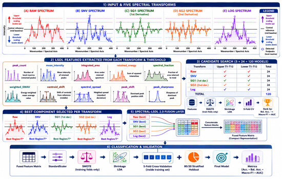
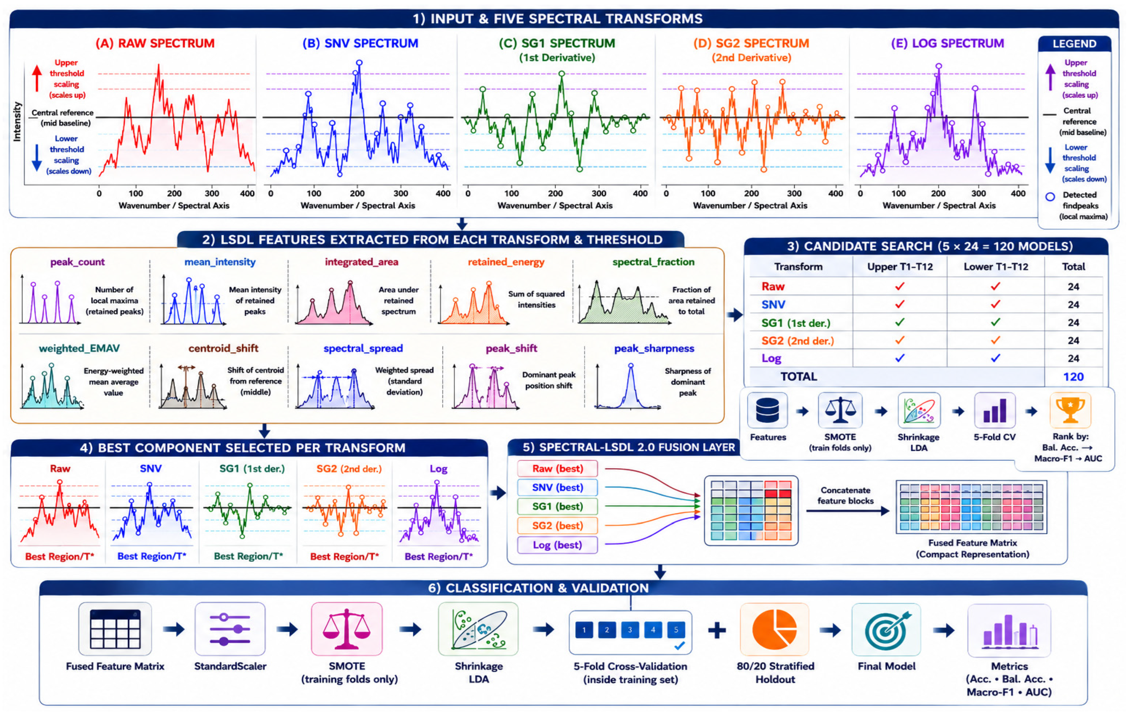
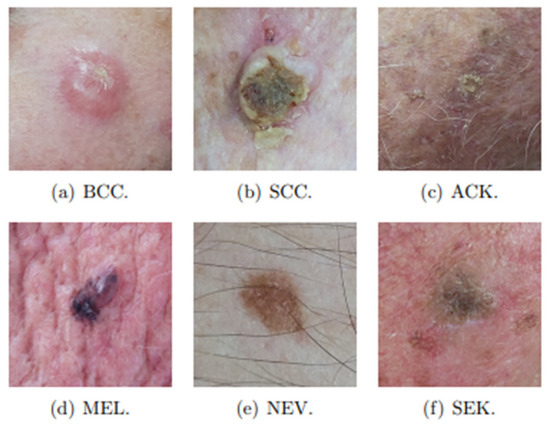
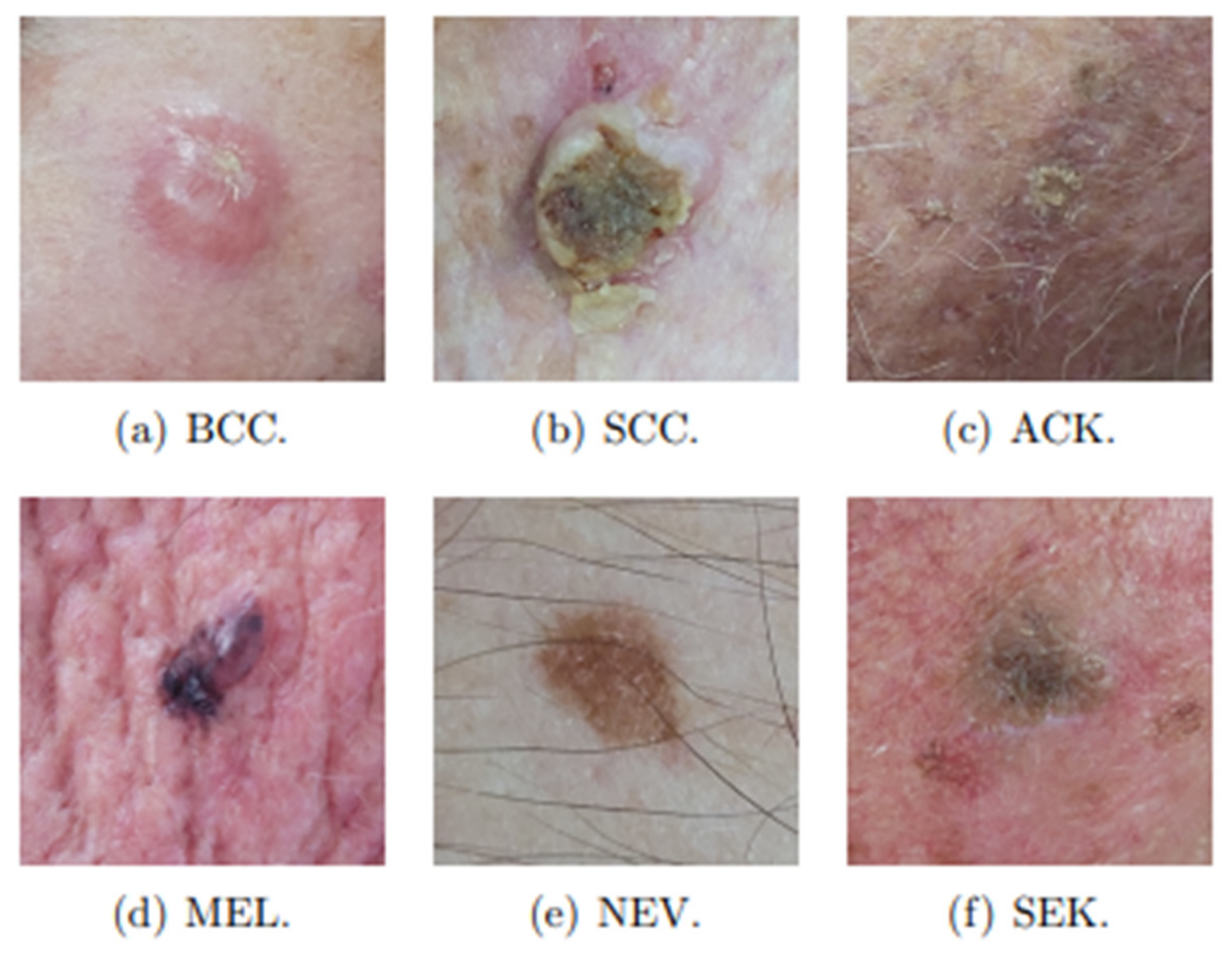
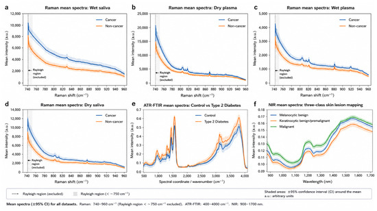
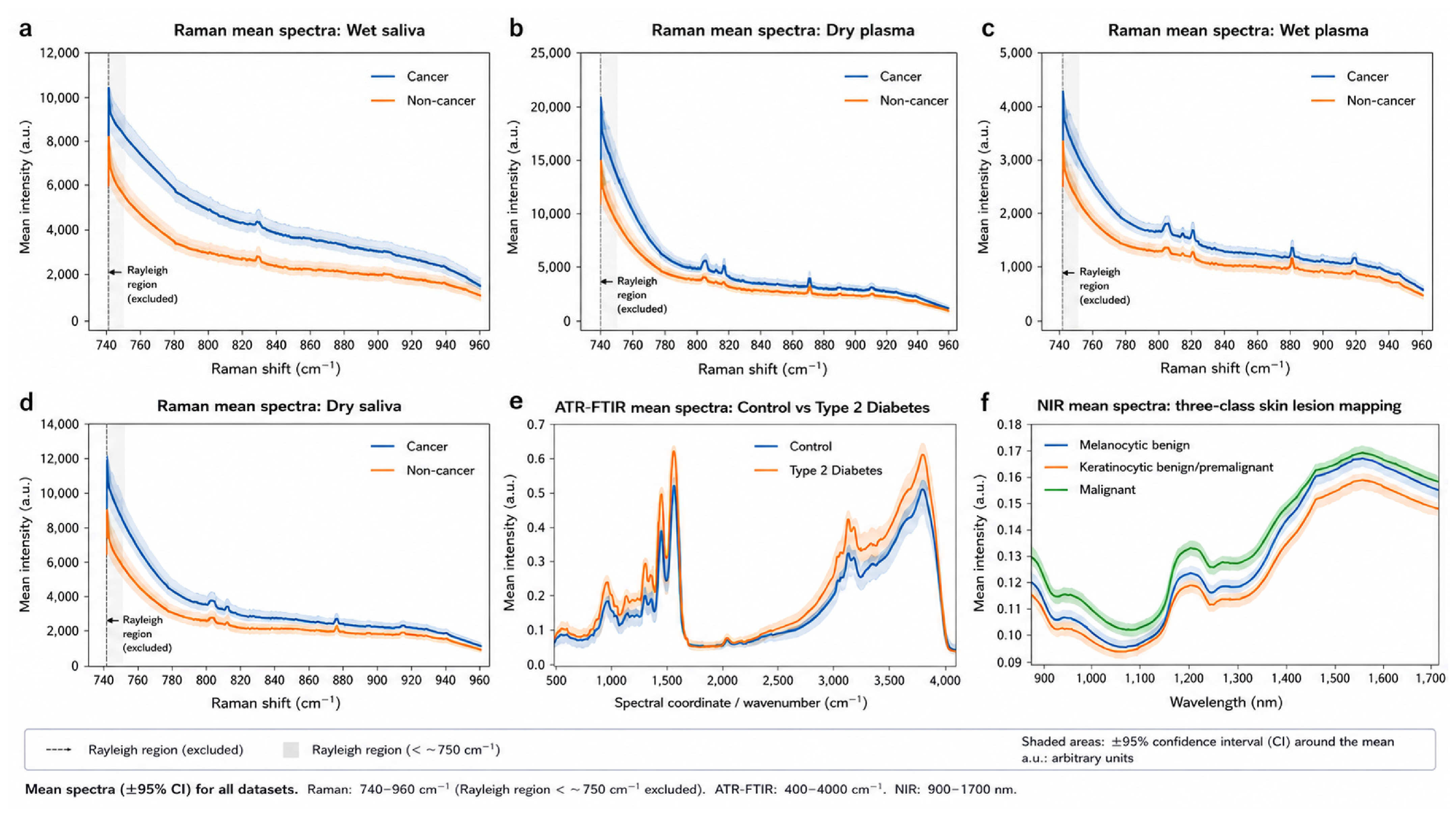
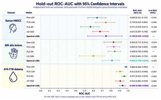
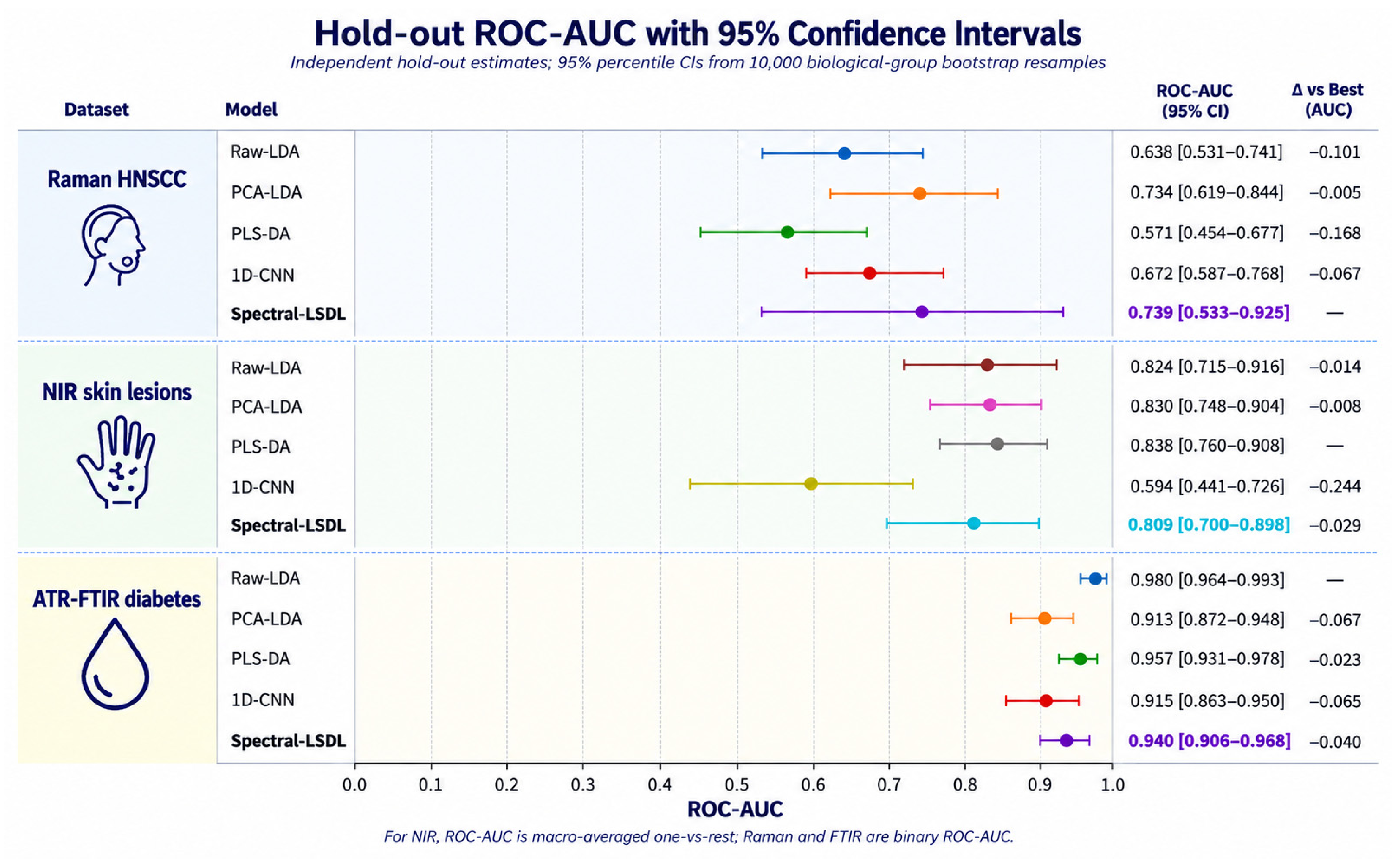
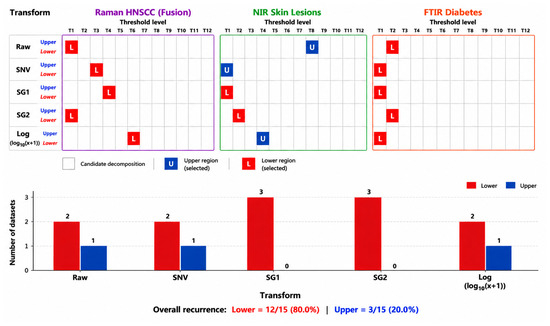
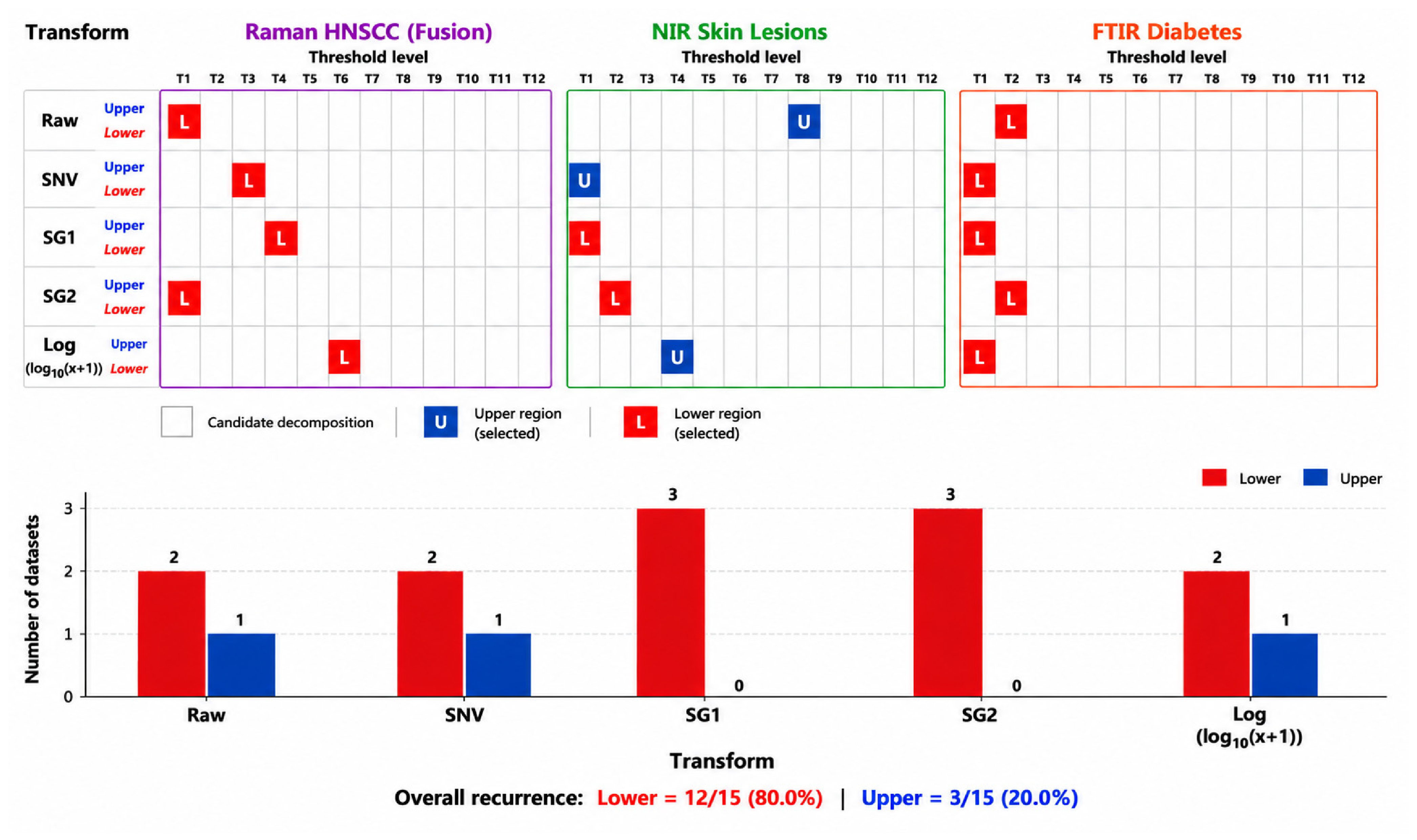

Disclaimer/Publisher’s Note: The statements, opinions and data contained in all publications are solely those of the individual author(s) and contributor(s) and not of MDPI and/or the editor(s). MDPI and/or the editor(s) disclaim responsibility for any injury to people or property resulting from any ideas, methods, instructions or products referred to in the content. |
© 2026 by the authors. Licensee MDPI, Basel, Switzerland. This article is an open access article distributed under the terms and conditions of the Creative Commons Attribution (CC BY) license.