


Abstract
The present paper is motivated by challenges in the design of the surface insulation in borehole thermal energy storage (BTES). A case study of a BTES with nine borehole heat exchangers (BHEs) in a cold climate is considered. Transient numerical modeling of the storage charging phase is performed by solving the three-dimensional heat equation using the finite difference method. Heat conduction through the insulation cover is simulated in accordance with Fourier’s law. A parametric study is conducted with respect to the prescribed heating setpoint temperatures in the BHEs and to the geometry of the insulation cover. The thermal analysis shows that the efficiency of the storage volume is strongly dependent on the heat transfer through the upper boundary. The insulation layer affects the minimum temperature reached within the BTES, with the influence of insulation thickness being most pronounced at thicknesses up to 10 cm. Furthermore, it is demonstrated that the lateral extension of the insulation cover has a greater impact on storage capacity gains than increasing its thickness, and that these energy gains expand progressively over time. Under cold ambient conditions, effective seasonal storage requires managing sharp ambient thermal gradients via a wider peripheral coverage of the insulation layer to offset vertical conductive losses.
1. Introduction
The global transition toward decentralized and carbon-neutral energy systems has intensified the need for large-scale Seasonal Thermal Energy Storage (STES) [1]. STES has assumed a crucial role in a wide range of engineering applications over recent decades, such as the recovery and utilization of waste heat [2], harvesting of renewable solar energy, increasing district heating networks capacity, etc. [3]. In combination with heat pumps, these systems can also support the balancing of electrical power grids [4] and, together with other energy storage technologies, contribute significantly to the ongoing transition toward smart energy grids [5]. Moreover, thermal energy accumulation is essential for reducing energy consumption in the building sector [6], particularly in buildings characterized by low thermal mass and limited storage capacity [7]. Although recent research has increasingly explored the integration of phase-change materials [7,8], the most mature and widely implemented solution remains sensible heat storage, primarily in water tanks, basins, and especially underground installations [9]. Such underground systems offer the advantage of saving valuable urban space and can be integrated into existing or planned infrastructure. Comparative assessments of state-of-the-art storage technologies identify sensible thermal energy storage as one of the most cost-effective and historically well-established solutions [10].
Despite their maturity and broad applicability, seasonal thermal energy storage systems are fundamentally limited by thermal losses occurring over extended storage periods. Comparative reviews of seasonal storage concepts, frequently integrated with heat pumps, identify heat loss mitigation as a key challenge and emphasize the influence of storage volume, geometry, and thermal boundary conditions on overall system performance [11]. Authoritative treatments of thermal energy storage further highlight the critical role of insulation strategies and boundary control in improving seasonal storage efficiency [12].
Among various technologies, BTES systems are particularly promising due to their ability to utilize the ground as a natural storage medium where large amounts of energy at a comparatively low price can be stored [13]. By storing surplus production sourced from solar collectors or industrial waste heat during periods of low demand and recovering it for space heating during winter, BTES offers a robust solution for balancing seasonal energy supply and demand [14]. Despite the inherent advantages of geothermal storage, the thermal efficiency of shallow BTES systems is significantly hampered by parasitic heat losses to the atmosphere. The top boundary of the storage volume, typically located in the unsaturated soil zone, is highly sensitive to ambient meteorological conditions and air temperature fluctuations [15]. Some authors recommend compact underground volumes [16], volumes with an appropriate aspect ratio [17], or a small storage surface footprint [18]. While the implementation of an insulating layer is a recognized engineering strategy to mitigate these losses, the complex, three-dimensional interaction between the evolving thermal plume and the insulating boundary requires detailed analysis [19].
Despite its structural importance, few studies isolate the geometric configuration of the top surface insulation as a primary variable in BTES performance. While existing literature identifies surface insulation as the second most critical factor governing heat retention after lateral ground conduction [16,20], detailed quantitative assessments of its geometry remain scarce. This thermal vulnerability is amplified in high-temperature BTES facilities operating at 55 °C or above [16]. Conventional analytical and numerical models frequently oversimplify this upper boundary condition, either by treating the ground surface as perfectly adiabatic, or by applying empirical, lumped heat-loss coefficients that neglect the explicit spatial and geometric features of the insulation cap [21]. In reality, high-temperature thermal storage drives a strongly transient, multi-dimensional heat flux that interacts dynamically with the local insulation thickness and coverage area before escaping to the surrounding environment.
While standard borehole models adequately simulate Ground Source Heat Pump (GSHP) operations based on heat-source inputs [22], they are less suited for high-temperature seasonal storage charging where the borehole wall temperature quickly stabilizes relative to the soil matrix along the BHE depth [23]. Many previous studies focus on environmental or operational parameters (e.g., [24]) rather than examining the influence of the surface insulation in particular. Most importantly, the existing literature lacks a systematic parametric evaluation that decouples the thermal benefits of the insulation’s horizontal coverage area from its vertical thickness under stable, cold-climate charging conditions. The present study directly addresses this research gap. We employ a three-dimensional transient heat conduction model [25,26] across a borehole array to isolate the specific geometric limits of the surface insulation. By examining a 180-day continuous charging phase at a constant ambient temperature, this work quantitatively maps how horizontal thermal gradients develop beneath the surface cap. The resulting parametric data establishes clear engineering thresholds for both insulation thickness and lateral footprint, providing concrete design criteria to minimize vertical parasitic losses in cold-climate seasonal storage.
To ensure the universality of the findings, the governing equation and boundary conditions are cast into a dimensionless form, allowing for a generalized assessment of storage performance through the Fourier number and dimensionless temperature ratios. The results provide critical insights into the optimization of insulating layers for shallow BTES, offering a design basis for maximizing heat retention in diverse climatic conditions.
2. System Configuration and Physical Model
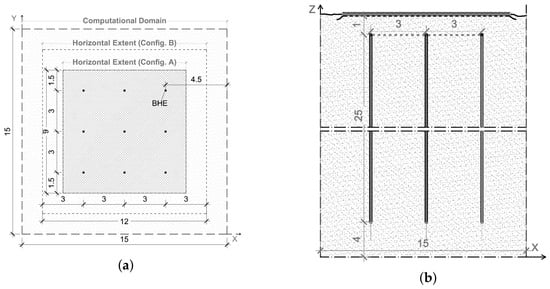
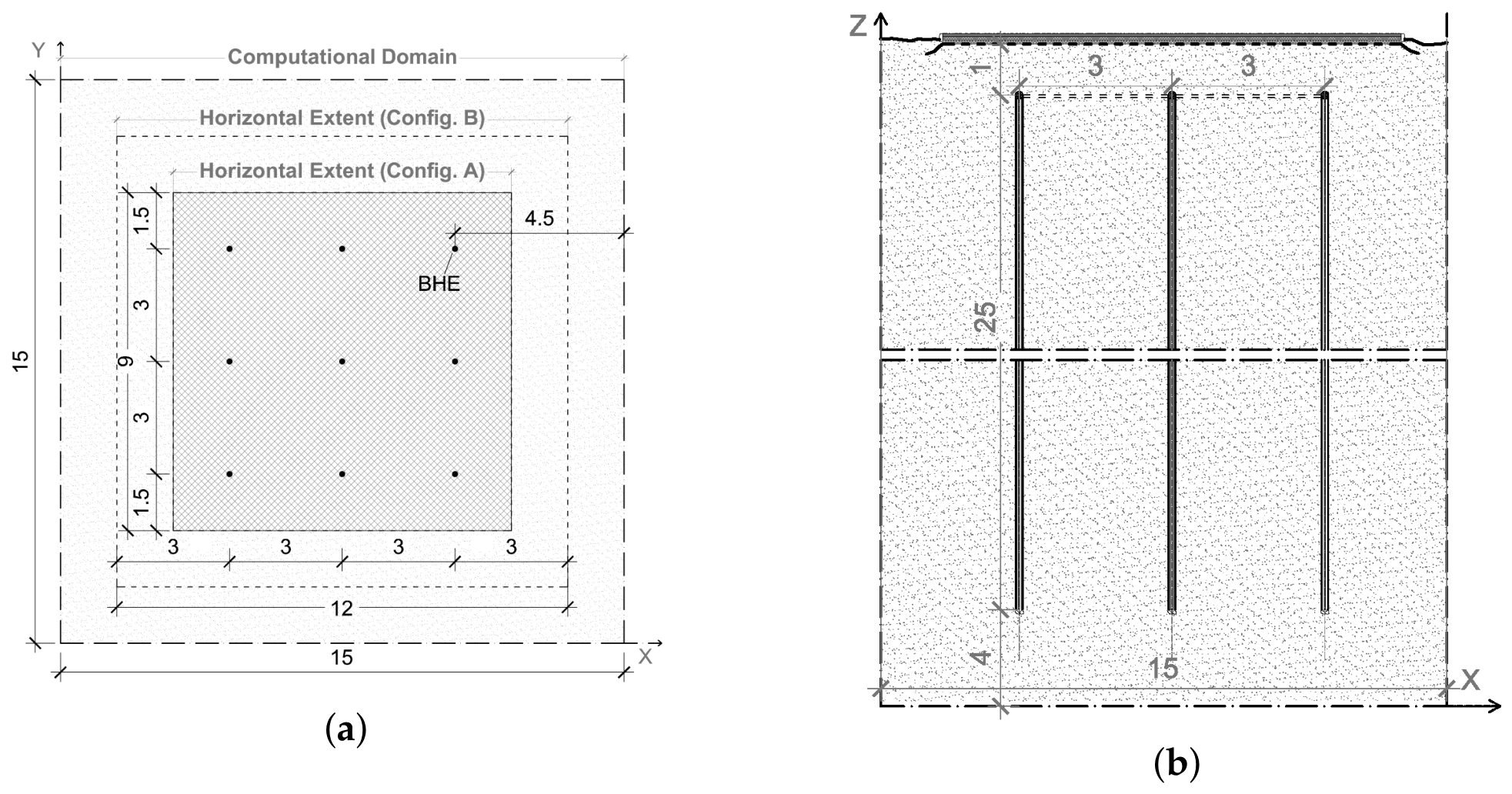
The BTES system considered in this study comprises a square array of nine BHEs, with a uniform spacing of between adjacent rows and columns (see Figure 1). Each borehole extends to a depth of , with the upper end positioned below the ground surface. To minimize thermal losses to the atmosphere, the top surface of the storage volume is protected by an insulating layer. This approach suppresses both atmospheric heat losses and external heat gains, thereby defining a centralized subsurface heat storage zone within the surrounding soil.
Figure 1.
Top view (a) and vertical cross-section (b) of the BTES field.
2.1. Mathematical Modeling and Numerical Simulations
In seasonal Borehole Thermal Energy Storage (BTES) systems, the charging phase occurs continuously over an extended macro-temporal horizon spanning several months. In the present numerical formulation, the thermal charging of the domain is not modeled as a volumetric heat source term in the governing differential equation. Instead, heat transfer into the soil matrix is governed by internal Dirichlet boundary conditions applied directly at the precise geometric coordinates of the boreholes, thereby omitting individual pipe fluid circuits. While circulating fluid temperatures fluctuate over short-term cycles, the average borehole wall boundary temperature approaches a quasi-steady equilibrium with the adjacent ground during prolonged, continuous charging. Imposing a fixed-temperature boundary condition enables a highly computationally efficient evaluation of macro-scale thermal plume development across the entire storage volume without the necessity of resolving sub-hourly, localized fluid loops. Imposing a Dirichlet boundary condition at the borehole wall assumes an idealized thermal connection, effectively treating the backfill and soil as a single medium with no contact resistance at the interface [27]. While this mathematical simplification causes a minor overestimation of heat transfer during the first few days of operation, it does not compromise the long-term results. As the seasonal thermal front expands into the storage field over months, the global heat storage capacity and long-term macro-scale temperature distributions remain highly representative.
The thermal behavior of the BTES system is characterized by the spatio-temporal evolution of the temperature field within the ground. The geological medium is assumed homogeneous and isotropic with constant material properties within the temperature range studied. As conduction is the dominant mode of heat transfer, the process is governed by the three-dimensional transient heat conduction equation. This approach allows the thermal energy propagation to be modeled as a pure diffusion process driven by the temperature gradients between the BHE surfaces and the surrounding soil medium. The governing equation is expressed as (e.g., [25,27]):
The notations used are as follows:
- are the spatial coordinates in the 3D Cartesian system [m];
- t is the time [s];
- denotes the transient 3D temperature distribution within the computational domain, [°C];
- is the effective thermal diffusivity of the ground, [].
An initial uniform temperature is prescribed throughout the computational domain. This same temperature is maintained at a far-field distance as a Dirichlet boundary condition on the bottom and domain lateral boundaries. The upper boundary, representing the insulating layer, is subjected to a constant ambient air temperature .
A third-type (Robin) boundary condition is applied at the exterior surface, utilizing a standardized external surface resistance to couple convective and radiative heat transfer with the ambient environment (shown in Section 2.2).
To generalize the findings and minimize the dependence on specific material properties, the governing equations are cast into a dimensionless framework. By introducing the characteristic length scale L equal to the BHE spacing of 3m, and the characteristic temperature difference , the spatial coordinates, time, and temperature are normalized. Here, represents the fixed heating setpoint temperature of the boreholes. The dimensionless variables are defined as follows:
Applying these transformations to Equation (1) yields the dimensionless heat conduction equation:
The thermal environment of the BTES system is defined by the following dimensionless conditions:
- Initial condition: The entire calculation domain is initialized at a uniform dimensionless temperature:
- Surface boundary: A constant value of is imposed at the top surface to represent the interface with the ambient air temperature ().
- Source: At the positions of the nine linear BHEs, the dimensionless temperature is maintained at , representing the active heating setpoint temperature .
- Far-field boundaries: The bottom and lateral boundaries of the domain are fixed at the undisturbed temperature to simulate the behavior of a semi-infinite medium.
Furthermore, to verify that the domain boundaries do not artificially distort the continuous thermal field, the far-field lateral and bottom Dirichlet boundary conditions (which prescribe a conservative scenario by acting as infinite thermal sinks) were compared against adiabatic Neumann zero-flux conditions along the same domain boundaries. The comparative analysis revealed that the solution for the temperature distribution within the reference storage volume remained completely invariant under both boundary types. This outcome demonstrates that the support of the transient thermal plume does not intersect the computational boundaries over the 180-day simulation horizon, thereby confirming that the selected domain dimensions are sufficiently large to preserve the intended semi-infinite physical assumptions and eliminate artificial boundary interference.
The Forward-Time Central-Space (FTCS) finite difference scheme is employed to solve Equation (3). The temporal derivative is approximated using a first-order explicit Euler method, while the spatial Laplacian operator is discretized using a second-order central difference scheme on a uniform Cartesian grid. This transformation yields the following explicit numerical recurrence relation:
subject to:
2.2. Insulating Layer Boundary Condition
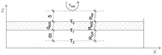
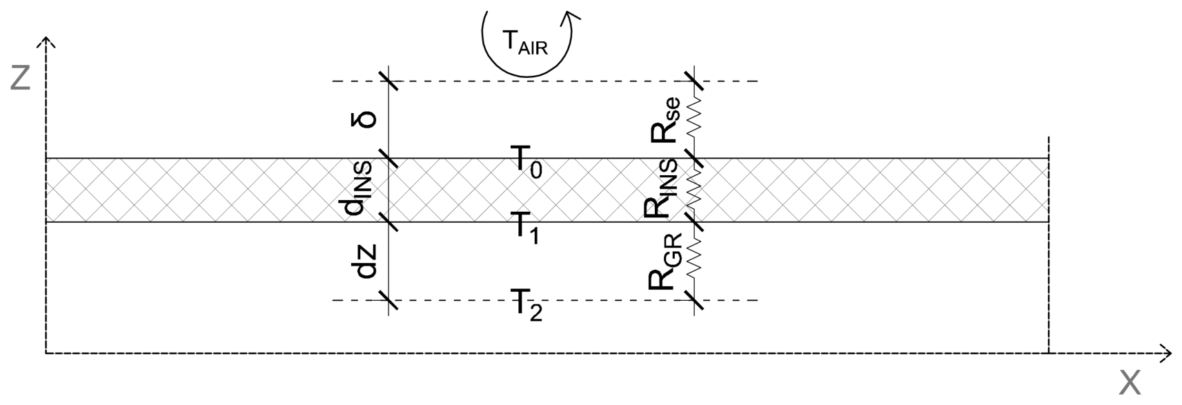
According to Equations (6) and (7) from [28], the time when axial heat losses become important for a single BHE (with physical characteristics described in Section 3) is approximately 100 days. For this reason and according to some good practices (e.g., [16,29,30]), the upper boundary is chosen to represent an insulating layer where the temperature is determined by a quasi-steady-state thermal resistance network. While the exterior air temperature is assumed constant to its mean value for the period, the temperature at the ground-insulation interface () is calculated through a heat balance at each time step, considering the thermal resistances and the temperatures and (shown in Figure 2 through their dimensional values):
where is the dimensionless temperature of the second computational node within the ground domain; f is the dimensionless thermal resistance weighting factor, defined as:
The individual thermal resistances are as follows:
Figure 2.
Schematic representation of the thermal resistance network used for the upper boundary condition at the surface insulation interface.
- is the thermal resistance of the top ground layer [], where is the thermal conductivity of the ground;
- is the thermal resistance of the insulation [], where and are the thickness and thermal conductivity of the insulation material, respectively;
- [] is the external surface heat transfer resistance related to the air boundary layer of thickness of an upward heat transfer flow, calculated according to the ISO 6946 standard [31]. accounts for the convective and radiative heat transfer at the exterior surface and ensures the model reflects standardized environmental boundary conditions.
The diagram in Figure 2 shows the corresponding dimensional temperatures (, , , ), the insulation thickness (), the external surface resistance (), and the vertical spatial increment (). This approach allows for a dynamic calculation of the top-surface heat loss as a function of the evolving internal ground temperature.
2.3. Model Verification, Numerical Stability, and Grid Independence
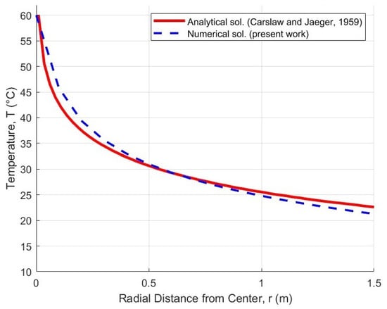
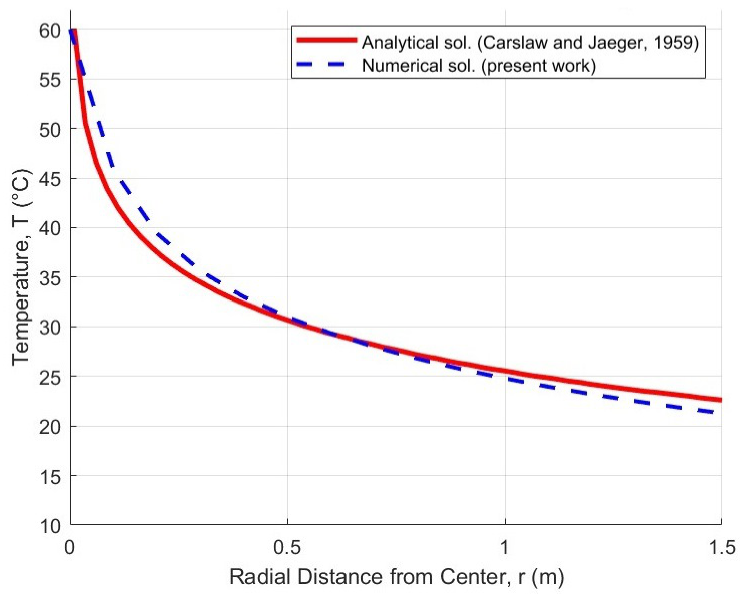
To ensure the algorithmic accuracy of the numerical scheme, researchers typically solve problems using multiple numerical methods or compare the results directly with exact analytical solutions [32]. The three-dimensional numerical code was simplified to a single-borehole domain to allow a direct comparison with the classical analytical solution for a cylinder operating under a constant wall surface temperature [33].
The verification simulation was executed with a charging temperature setpoint () of 60 °C and an initial undisturbed ground temperature () of 12 °C. To minimize upper and lower boundary edge effects, the evaluation was conducted at the mid-depth plane of the borehole. The ground temperature was monitored at a radial distance of from the borehole wall, corresponding to the mid-spacing distance between adjacent heat exchangers in the full BTES array. After a transient simulation period of 180 days, the spatial temperature profiles from the numerical model and the analytical solution were compared (Figure 3). The resulting Mean Absolute Percentage Error (MAPE) was . This close agreement verifies that the numerical scheme is mathematically correct and possesses sufficient precision to reliably capture the macro-scale transient heat conduction within the storage field.
Figure 3.
Model verification with an exact analytical solution [33] after 180 days.
To ensure the convergence and reliability of the numerical results, the selection of the discretization parameters must adhere to the fundamental limits of the explicit finite-difference framework. For the three-dimensional FTCS scheme, the von Neumann stability analysis dictates a strict upper bound on the time step to prevent the amplification of numerical oscillations. In the dimensionless domain, this stability condition is expressed as follows:
In the context of the physical dimensions, where h represents a uniform spatial step (), the dimensional stability condition translates to:
A grid independence study was conducted to establish an optimal balance between computational execution time and solution accuracy. The numerical sensitivity of the spatial discretization was evaluated over a 10-day operational sample period. For spatial grid steps of 0.05 m, 0.10 m and 0.20 m, the computed minimum temperatures within the BTES domain were 9.74 °C, 9.82 °C and 9.96 °C, respectively. Performance profiling indicated an approximate ninefold increase in total wall-clock execution time for each twofold reduction in spatial step size, driven by the stricter time-step stability constraints of the explicit solver. Relative to the finest mesh (0.05 m), the maximum deviation in the minimum temperature reached 2.3% for the 0.20 grid, whereas the 0.10 grid restricted this deviation to just 0.8%. Consequently, a uniform grid spacing of 0.10 was selected as it yields an optimal trade-off between numerical accuracy and computational efficiency, aligning with established convergence thresholds in literature [20]. For the final m computational domain which houses nine boreholes with individual depths of 25 m this spatial resolution results in a total discretization mesh of approximately nodes.
3. Results
To evaluate a physically representative case study under cold-climate constraints, the dimensionless governing equations are evaluated across a computational domain scaled from a baseline physical field configuration. This reference domain measures m (length, width, and depth, respectively) and hosts the borehole heat exchanger (BHE) array geometry illustrated in Figure 1. The total simulated charging period corresponds to a physical time of s (approximately 180 days), mapped into the solver via the dimensionless time variable (). Subsurface thermal transport is scaled using the effective properties of a saturated silty-clay geological formation. The medium is characterized by a baseline thermal conductivity = 1.7 W/(mK) and a thermal diffusivity = 4 /s, assuming a saturated matrix porosity of 0.4. These effective properties are calculated using Lichtenecker’s geometric mixing rule for conductivity and a volumetric weighted average for heat capacity. The effective heat capacity , implied by the relationship , is approximately 4.25 × 10⁶ J/(K), consistent with the high volumetric heat capacity of water-saturated storage volumes. The thermal environment is defined by an undisturbed ground temperature °C and an ambient air temperature °C. The exterior air temperature is maintained throughout the simulated period, and it reflects the approximate daily average outdoor temperature throughout the studied 180 days. The choice to use a constant time-averaged temperature boundary condition for the whole period is a deliberate modeling abstraction justified by the ground damping effect (soil thermal inertia dampening diurnal short-term fluctuations) and the macro-scale focus of the simulations. For such macro-scale evaluations, using a conservative, seasonal mean ambient temperature provides highly reliable thermal efficiency metrics while maintaining computational tractability. The specifically chosen value is the most conservative cold-climate estimation for ambient conditions of underground thermal energy storage research location in Europe [34], namely in Longyearbyen, Norway.
To assess the thermal storage potential of the system, a reference storage volume is defined. The lateral extent of this volume projects 1.5 m beyond the outermost borehole centers in all directions, corresponding to half the borehole spacing. This results in a m region with a total volume of . Based on the effective material properties of the ground, the heat capacity of this region is MWh/K. The stored thermal energy within the reference volume is quantified as
where is the average temperature calculated from the nodal values within the reference volume. This metric provides a bulk measure of the thermal energy retained in the subsurface relative to the initial state. While this definition does not account for extraction efficiency or thermal losses during discharge, it enables consistent comparison of storage performance across different insulation configurations.
3.1. Operational Parameters and Insulation Configurations
The parametric study investigates the thermal response of the storage volume under varying heat injection regimes and surface insulation strategies. The BHEs are modeled using a constant temperature boundary condition, with setpoint temperatures () ranging from 40 °C to 90 °C. To evaluate the effectiveness of the surface thermal barrier, the insulation thickness () is varied from (representing a non-insulated baseline) to .
Furthermore, the study assesses the impact of the lateral extension of the insulation cover. Two distinct geometric configurations are compared to determine the optimal peripheral protection:
- Configuration A: a cover extending beyond the outermost BHEs, providing a moderate thermal buffer.
- Configuration B: a cover extending beyond the peripheral heat exchangers, designed to further minimize lateral heat dissipation at the surface.
These parameters allow for the quantification of heat retention efficiency as a function of both the thermal resistance and the spatial coverage of the insulation.
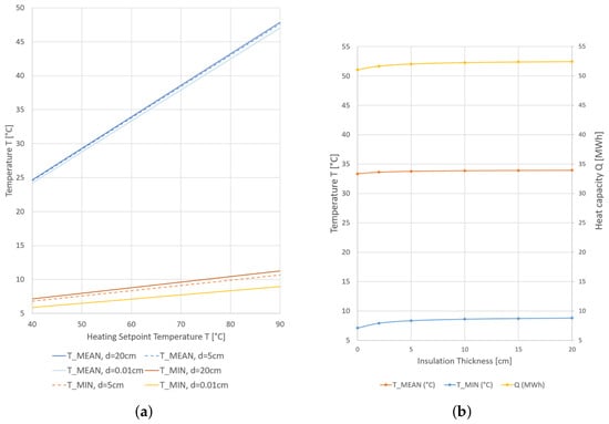
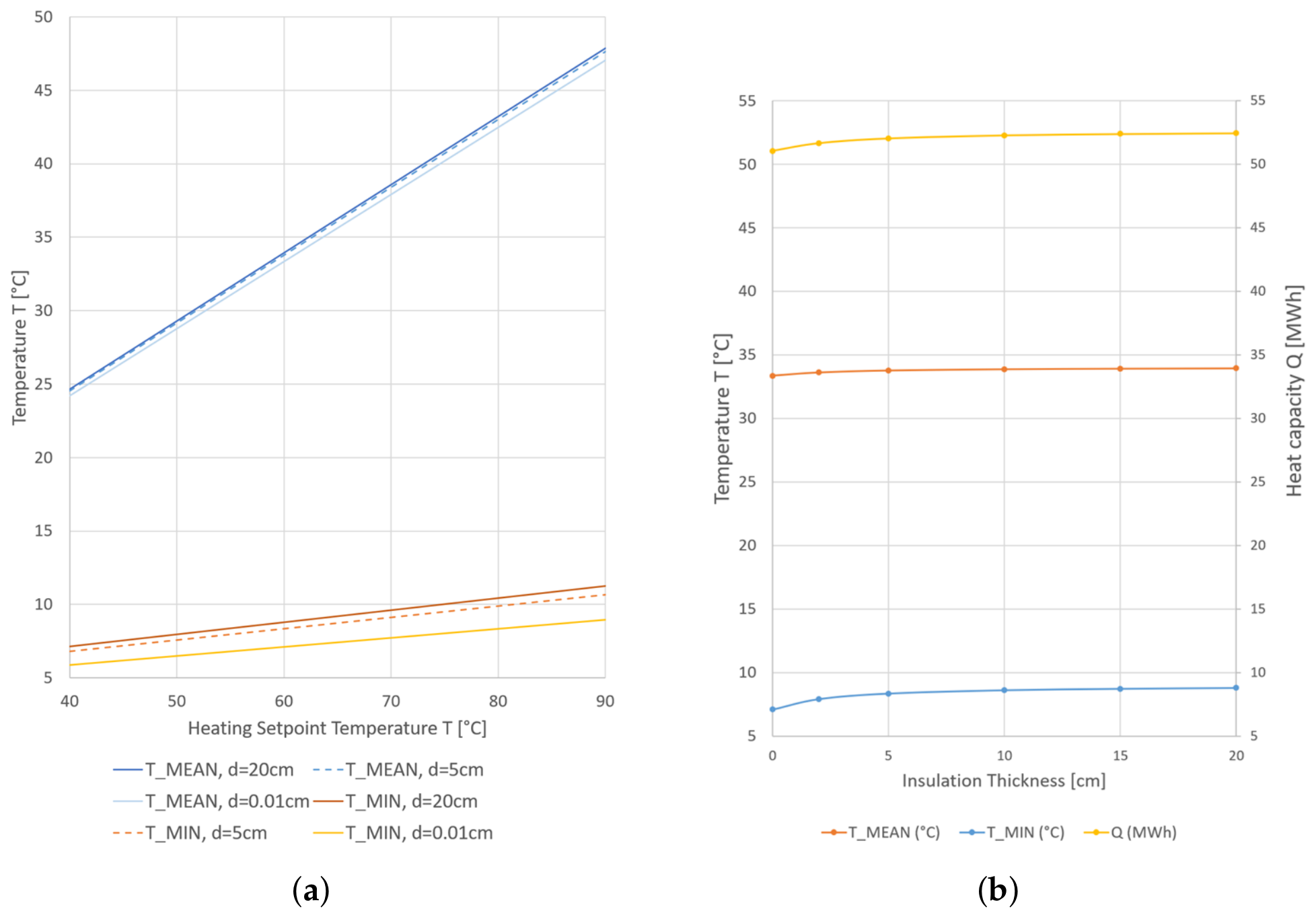
Figure 4 shows average and minimum temperatures and storage capacity as functions of heating setpoint temperature and insulation thickness for configuration A scenario. The simulated thermal fields indicate that both the average temperature () and minimum storage temperature () exhibit a linear correlation with the applied BHE setpoint temperature (Figure 4a). The sensitivity of the temperature distribution to the surface boundary condition varies spatially with most pronounced effect of the insulating layer in the vicinity of the minimum temperature zones, located in the shallowest subsurface layers. Due to their proximity to the top surface, these regions are subject to higher thermal gradients and are therefore more sensitive to the thermal resistance of the insulation layer. Consequently, increasing the insulation thickness significantly elevates the minimum temperature threshold, effectively stabilizing the storage volume against atmospheric cooling.
Figure 4.
(a) Average and minimum temperatures as functions of heating setpoint temperature and insulation thickness (Configuration A scenario). (b) Average and minimum temperatures and total storage capacity for varying insulation thicknesses at a heating setpoint temperature of 60 °C. (Configuration A scenario).
Table 1 and Table 2 show minimum and average temperatures and storage capacity for both configurations of the insulation cover at heating setpoint temperature of 60 °C. Increasing the thickness of the insulation cover to mitigate surface thermal losses up to 20 cm augments the net thermal energy storage capacity by 2.76% under a 9 × 9 m insulation footprint, and by 3.76% when the cover footprint is expanded to 12 × 12 m. However, the increase in thickness clearly demonstrates the law of diminishing returns. Scaling the thickness from 0 to 5 cm captures a prominent capacity gain (+1.94% for Configuration A). Moving from 5 cm to 10 cm yields a small but noticeable marginal benefit of +0.48%. Nevertheless, doubling the insulation further from 10 cm to 20 cm results in an engineering plateau (Figure 4b), providing a negligible incremental capacity increase of just +0.33% (0.17 MWh). From an economic perspective, doubling the material volume beyond 10 cm is entirely unjustified by this nominal heat retention, establishing 10 cm as the optimal design threshold. The true engineering significance of this variation is not found in the bulk capacity metric, but rather in the thermal stabilization of the reference storage volume. As shown by the temperature rows, the wider peripheral coverage (Configuration B) at 10 cm thickness drives the minimum storage temperature () upward by 4.43 °C (shifting from 8.62 °C to 13.05 °C, a relative increase of 51.4%).
Table 1.
Temperatures and storage capacity for Configuration A (9 × 9 m insulating layer) at a heating setpoint temperature of 60 °C for different insulation thicknesses.
Table 2.
Temperatures and storage capacity for Configuration B (12 × 12 m insulating layer) at a heating setpoint temperature of 60 °C for different insulation thicknesses, including the gain in storage capacity relative to Configuration A (9 × 9 m insulating layer).
It is interesting to observe that the spatial coverage of the insulation further beyond the useful storage volume (configuration B) has a significant effect on the thermal losses. Comparing the numerical results from Table 1 and Table 2 for insulation covers of 9 × 9 × 0.15 m and 12 × 12 × 0.05 m, the average temperature (approx. 33.91 °C) and storage capacity (approx. 52.38 MWh) are almost equal; however, the 12 × 12 × 0.05 m solution is using 40% less insulation resulting in higher material-effectiveness (hence, cost-effectiveness). This shows that insulating further from the actual boreholes can have a stronger effect on minimizing thermal losses than merely increasing the insulation thickness. The practical implication for the design engineer is to prioritize the lateral extension of the insulation cover, ensuring it projects outward by at least one full borehole spacing (Configuration B) beyond the perimeter of the outermost boreholes in the BTES array.
3.2. Transient Thermal Evolution, Storage Capacity and Energy Gains
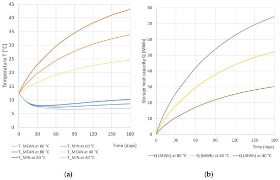
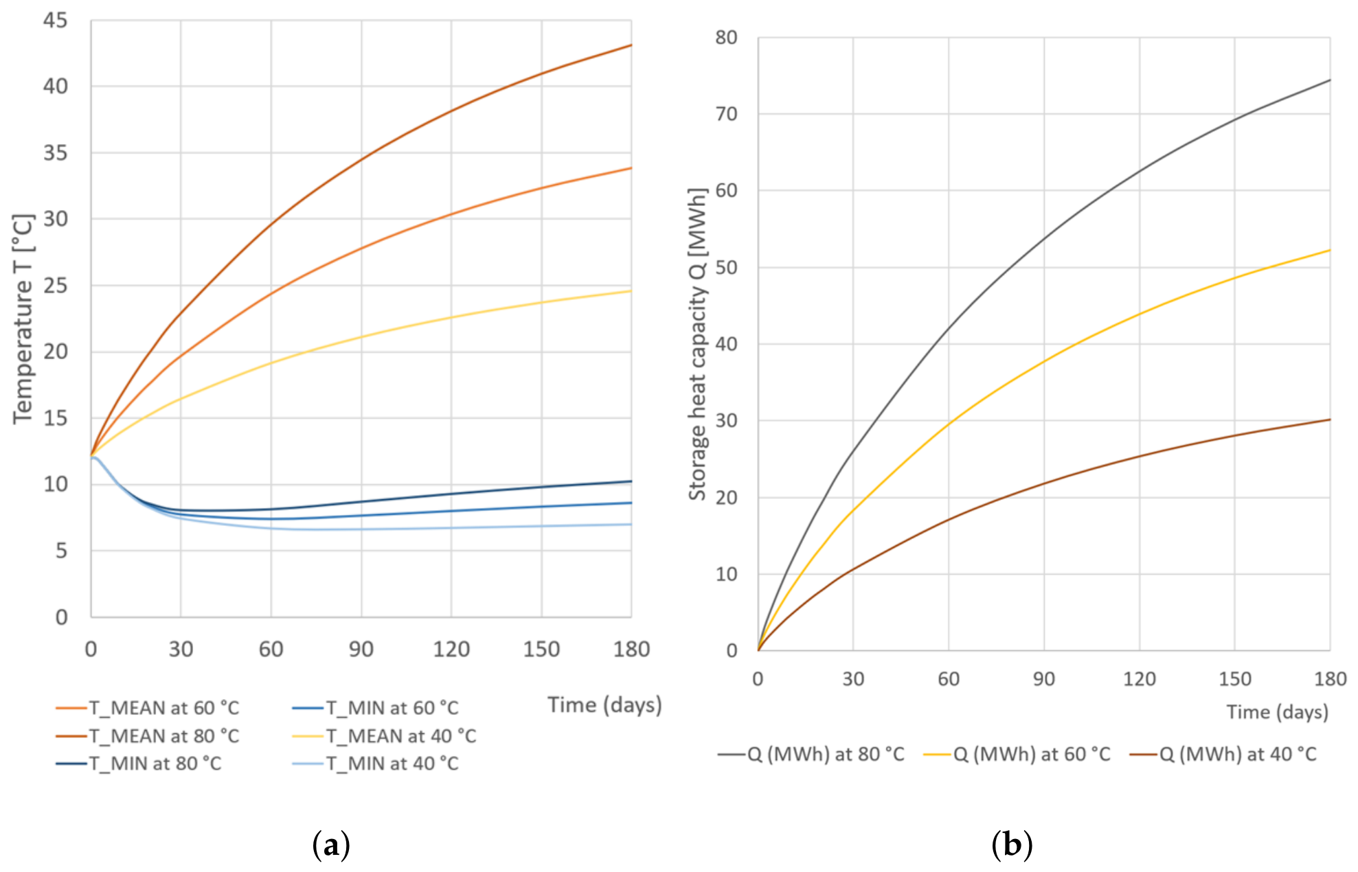
The dynamic thermal behavior of the BTES system is illustrated in Figure 5, which depicts the evolution of the temperature profiles and storage capacity for setpoint temperatures of 40 °C, 60°C, and 80 °C at a constant insulation thickness of 10 cm and lateral dimensions of 9 × 9 m.
Figure 5.
Transient evolution of average and minimum storage temperatures (a) and cumulative heat storage capacity (b) for varying BHE setpoint temperatures (40 °C, 60 °C and 80 °C) with a surface insulation area of 9 × 9 m and 10 cm insulation thickness.
Beginning from a uniform initial ground temperature of 12 °C, the minimum temperature within the storage domain exhibits an initial decline before entering a phase of gradual recovery (Figure 5a). This initial drop is attributed to the thermal lag and the cooling influence of the upper boundary before the heat plume from the BHEs fully penetrates the peripheral zones. The minimum temperatures reach values as low as 7.10 °C in Configuration A of the insulating cover and 7.43 °C in Configuration B (Table 1 and Table 2). Notably, under the prescribed insulation, the minimum temperature remains below the initial 12 °C baseline throughout the 180-day injection cycle, regardless of the setpoint temperature. This suggests that while surface insulation mitigates heat loss, a thermal deficit persists at the boundaries of the array within this timeframe. In this regard, the competitive behavior between the environmental cold front and the artificial thermal plume from the BHEs during the initial operational phase of the multi-year BTES may result in engineering challenges, such as the triggering of localised soil frost, which could have an adverse effect on subsequent heat extraction efficiency.
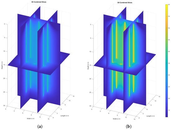
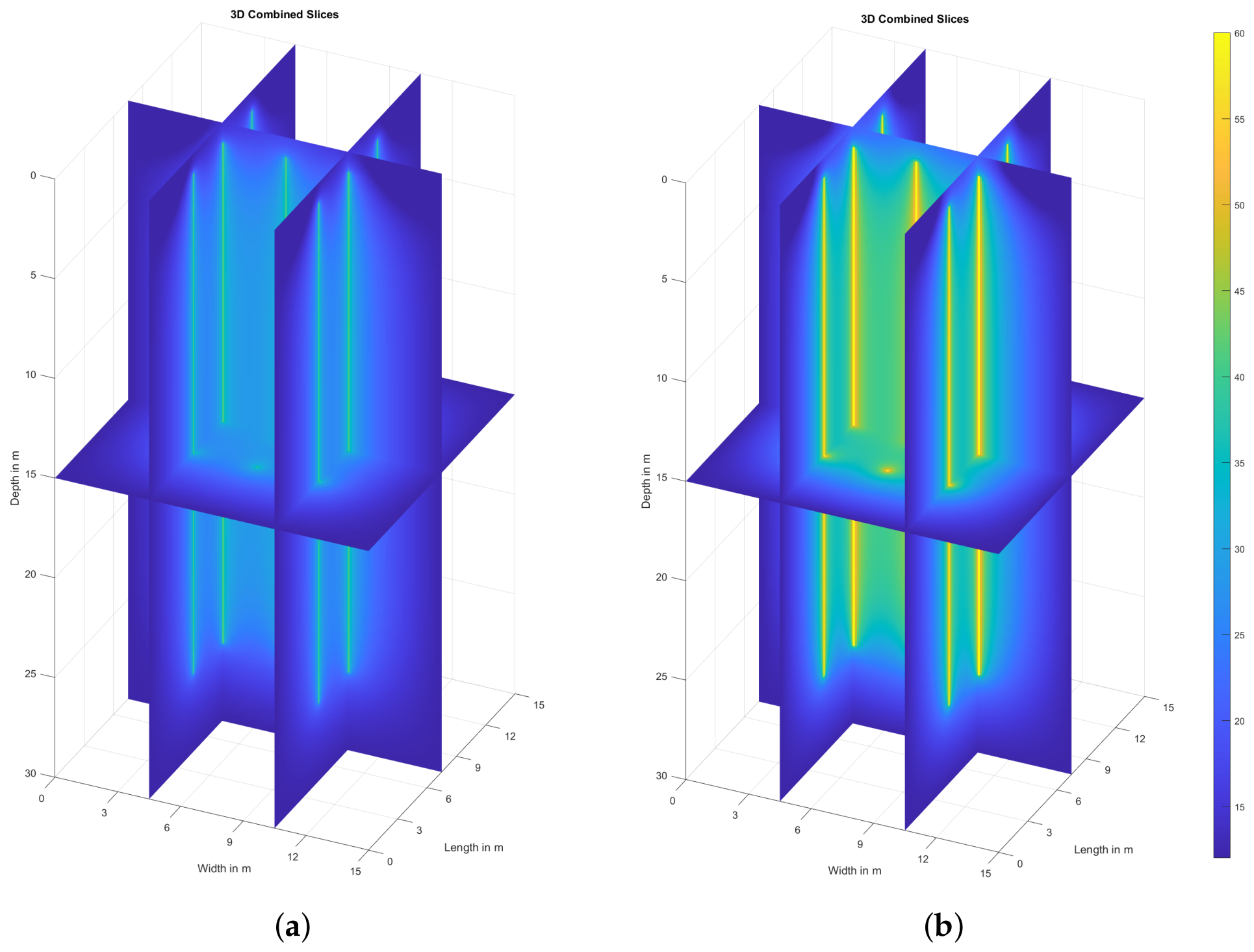
The accumulation of thermal energy, represented by the total BTES capacity in Figure 5b, directly correlates with the rise in the average storage temperature in Figure 5a. This quasi-parabolic increase in energy density reflects the steady-state heat injection process. The spatial variability of these results is further detailed in Figure 6, which provides the cross-sectional temperature distributions for the 40 °C and 60 °C scenarios at the end of the simulation period.
Figure 6.
Three-dimensional temperature distributions after 180 days for heating setpoint temperatures of 40 °C (a) and 60 °C (b). Both cases assume a m surface insulation area with a thickness of 10 cm.
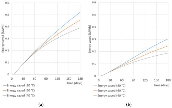
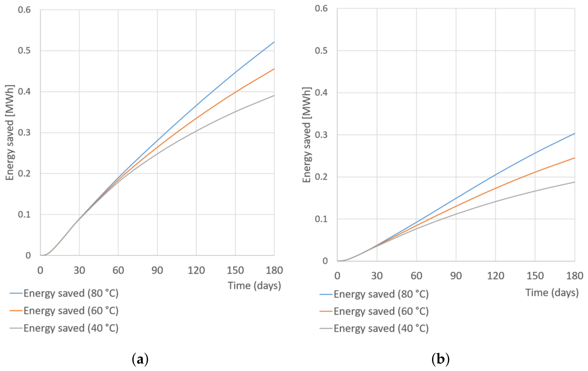
Figure 7a shows the storage capacity gains due to the extension of the cover area comparing Configuration A with Configuration B at an insulation thickness of 10 cm. Figure 7b demonstrate the effect of the increase of the insulation thickness on the storage capacity gains for Configuration A. Comparing the behavior of 12 × 12 × 0.10 m storage cover with a 9 × 9 × 0.10 m one, the energy savings are larger for BTES with higher temperature setpoints (Figure 7a). Similar results are obtained for doubling the insulation thickness (Figure 7b). As indicated by Table 1 and Table 2, storage capacity gains increase more rapidly when extending the lateral dimensions of the cover than when increasing its thickness. This effect actually pertains to the edge dynamics of the 3D thermal plume near the surface and the severing of lateral heat dissipation paths. As seen in Figure 7, storage capacity gains for different heating setpoint temperatures remain marginal during the initial stabilization phase (between 40 and 60 days). Afterwards, a performance inflection occurs and the cumulative thermal benefits expand substantially in high-temperature regimes. It is also obvious that in both practical cases, the gains related to the axial thermal losses increase significantly over time, just as predicted by the analytical formulas derived in [28].
Figure 7.
Stored energy gains over time for different surface insulation designs at heating setpoint temperatures of 40, 60, and 80 °C. (a) Effect of extending the surface insulation cover area (Configuration B relative to Configuration A) at an insulation thickness of 10 cm. (b) Effect of increasing the surface insulation layer thickness from 5 cm to 10 cm for Configuration A.
4. Discussion
The numerical results reveal a complex thermal interaction between high-temperature injection at the BHEs and the cooling influence of the upper boundary. The observed initial decrease in the minimum BTES temperature serves as a critical indicator of the system’s transient thermal lag. Given that the ambient air temperature ( °C) is assumed lower than the undisturbed ground temperature ( °C), a cooling front propagates downward from the surface at the onset of the simulation.
This cooling effect competes with the radial heat propagation originating from the borehole array. Regardless of the heating setpoint temperature and the insulation thickness, for limited surface coverage of the insulation, the injected thermal power proves insufficient to counteract the heat flux lost through the upper boundary during the first charging cycle. Consequently, the zone just beneath the storage cover where the minimum temperature is recorded experiences a net thermal deficit relative to its initial state.
Furthermore, the ’reference storage volume’ concept enables a consistent quantification of energy density across different system configurations, including variations in setpoint temperature, insulation thickness, and insulation surface area. The results suggest that for shallow BTES systems, the surface insulation layer functions not merely as an auxiliary component but as a primary determinant of storage viability. Without high-performance insulation, low-temperature thermal energy cannot be effectively stored, as vertical conductive losses negate the gains from seasonal injection.
5. Conclusions
This parametric study establishes the principal relationship between injection temperatures and surface insulation for shallow BTES systems. The primary outcomes are summarized as follows:
- Optimal insulation thickness: A distinct trend of diminishing returns occurs for insulation thicknesses exceeding . For standard operational setpoints, increments beyond this threshold yield negligible improvements in thermal recovery ratios.
- Influence of lateral insulation extension: The simulations demonstrate that the lateral extension of the insulation layer provides greater storage capacity gains than increasing its thickness alone. Prioritizing the lateral extension of the insulation cover to at least one full borehole spacing beyond the outermost borehole perimeter, rather than merely increasing insulation thickness, enhances the material effectiveness and, consequently, the cost-effectiveness of the storage design.
- Operational constraints: An insulation cover with an insufficient footprint proves inadequate for maintaining the entire reference storage volume above its undisturbed ground temperature under cold ambient conditions, regardless of the investigated insulation thicknesses or heating setpoint temperatures. Within the studied timeframe, a thermal deficit beneath the insulating layer persists due to the pronounced thermal lag of the heat plume from the borehole heat exchangers.
- Design sensitivity: Thermal sensitivity analysis reveals that the efficiency of the storage volume depends heavily on the top insulating layer. While storage capacity gains for different heating setpoint temperatures remain marginal during the initial stabilization phase, a significant performance inflection occurs, and the cumulative thermal benefits expand substantially in high-temperature regimes. Finally, the lateral extension of the peripheral insulation contributes significantly to thermal stabilization of the storage and to the reduction of surface edge conduction losses.
Author Contributions
Conceptualization, M.R., S.S. and M.D.; Methodology, M.R., S.S. and M.D.; Software, M.R.; Validation, R.S. and G.R.; Formal analysis, S.S. and M.D.; Writing—original draft, M.R., S.S. and M.D.; Writing—review and editing, M.R., S.S., G.R., R.S. and M.D.; Visualization, M.R.; Supervision, S.S. and M.D.; Project administration, M.D. and G.R.; Funding acquisition, G.R., R.S. and M.D. All authors have read and agreed to the published version of the manuscript.
Funding
This research was supported by the European Union NextGenerationEU through the National Recovery and Resilience Plan of the Republic of Bulgaria, Project BG-RRP-2.017-0036-C01 “Seasonal and short-term thermal energy storage system with geothermal heat exchangers and phase change materials using renewable energy sources”.
Data Availability Statement
The original contributions presented in this study are included in the article. Further inquiries can be directed to the corresponding author.
Acknowledgments
Maria Datcheva acknowledges the access to the infrastructure provided through Project BG16RFPR002-1.014-0018-C01 “Centre of Excellence in Informatics and ICT” financed by the Science and Education for Smart Growth Operational Program and co-financed by the European Union through the European Structural and Investment Funds.
Conflicts of Interest
The authors declare no conflicts of interest. The funders had no role in the design of the study; in the collection, analyses, or interpretation of data; in the writing of the manuscript; or in the decision to publish the results.
Abbreviations
The following abbreviations are used in this manuscript:
| BHE | Borehole Heat Exchanger |
| BTES | Borehole Thermal Energy Storage |
| FTCS | Forward-Time Central-Space |
| STES | Seasonal Thermal Energy Storage |
References
- Lund, H.; Werner, S.; Wiltshire, R.; Svendsen, S.; Thorsen, J.E.; Hvelplund, F.; Mathiesen, B.V. 4th Generation District Heating (4GDH): Integrating smart thermal grids into future sustainable energy systems. Energy 2014, 68, 1–11. [Google Scholar] [CrossRef] [Scilit]
- Miro, L.; Gasia, J.; Cabeza, L.F. Thermal energy storage (TES) for industrial waste heat (IWH) recovery: A review. Appl. Energy 2016, 179, 284–301. [Google Scholar] [CrossRef] [Scilit]
- Dahash, A.; Oxe, F.; Janetti, M. Advances in seasonal thermal energy storage for solar district heating applications: A critical review on large-scale hot-water tank and pit thermal energy storage systems. Appl. Energy 2019, 239, 296–315. [Google Scholar] [CrossRef] [Scilit]
- Enescu, D.; Chicco, G.; Porumb, R.; Seritan, G. Thermal energy storage for grid applications: Current status and emerging trends. Energies 2020, 13, 340. [Google Scholar] [CrossRef] [Scilit]
- Tan, K.M.; Babu, T.S.; Ramachandaramurthy, V.K.; Kasinathan, P.; Solanki, S.G.; Raveendran, S.K. Empowering smart grid: A comprehensive review of energy storage technology and application with renewable energy integration. J. Energy Storage 2021, 39, 102591. [Google Scholar] [CrossRef] [Scilit]
- Lizana, J.; Chacartegui, R.; Barrios-Padura, A.; Valverde, J.M. Advances in thermal energy storage materials and their applications towards zero energy buildings: A critical review. Appl. Energy 2017, 203, 219–239. [Google Scholar] [CrossRef] [Scilit]
- Bai, L.; Xie, J.; Farid, M.M.; Wang, W.; Liu, J. Analytical model to study the heat storage of phase change material envelopes in lightweight passive buildings. Build. Environ. 2020, 169, 106531. [Google Scholar] [CrossRef] [Scilit]
- Zohra, M.; Riad, A.; Alhamany, A.; Sennoune, M.; Mansouri, M. Improvement of thermal energy storage by integrating PCM into solar system. J. Therm. Eng. 2020, 5, 816–828. [Google Scholar] [CrossRef] [Scilit]
- Novo, A.V.; Bayon, J.R.; Castro-Fresno, D.; Rodriguez-Hernandez, J. Review of seasonal heat storage in large basins: Water tanks and gravel–water pits. Appl. Energy 2010, 87, 390–397. [Google Scholar] [CrossRef] [Scilit]
- Xu, J.; Wang, R.Z. A review of available technologies for seasonal thermal energy storage. Sol. Energy 2014, 103, 610–638. [Google Scholar] [CrossRef] [Scilit]
- Hesaraki, A.; Holmberg, S.; Haghighat, F. Seasonal thermal energy storage with heat pumps and low temperatures in building projects—A comparative review. Renew. Sustain. Energy Rev. 2015, 43, 1199–1213. [Google Scholar] [CrossRef] [Scilit]
- Dincer, I.; Rosen, M.A. Thermal Energy Storage: Systems and Applications; John Wiley & Sons: Hoboken, NJ, USA, 2011. [Google Scholar]
- Hellström, G. Ground Heat Storage: Thermal Analyses of Duct Storage Systems; University of Lund: Lund, Sweden, 1991. [Google Scholar]
- Schmidt, T.; Mangold, D.; Müller-Steinhagen, H. Central solar heating plants with seasonal storage in Germany. Sol. Energy 2004, 76, 165–174. [Google Scholar] [CrossRef] [Scilit]
- Catolico, N.; Ge, S.; McCartney, J.S. Numerical modeling of a soil-borehole thermal energy storage system. Appl. Energy 2016, 181, 44–55. [Google Scholar]
- Kvalsvik, K.H.; Ramstad, R.K.; Holmberg, H.; Kocbach, J. Measurements and simulations of high temperature borehole thermal energy storage in Drammen, Norway—Evaluation of thermal losses and thermal barrier. Geothermics 2025, 125, 103192. [Google Scholar]
- Rashevski, M. Influence of the aspect ratio on the thermal stratification in underground sensible thermal energy storage. J. Theor. Appl. Mech. 2025, 55, 52–62. [Google Scholar] [CrossRef] [Scilit]
- Skarphagen, H.; Banks, D.; Frengstad, B.S.; Gether, H. Design considerations for borehole thermal energy storage (BTES): A review with emphasis on convective heat transfer. Geofluids 2019, 2019, 4961781. [Google Scholar] [CrossRef] [Scilit]
- Dahash, A.; Ochs, F.; Tosatto, A.; Streicher, W. Toward efficient numerical modeling and analysis of large-scale thermal energy storage for renewable district heating. Appl. Energy 2020, 279, 115840. [Google Scholar] [CrossRef] [Scilit]
- Pokhrel, S.; Amiri, L.; Poncet, S. Reduced order 1+3D numerical model for evaluating the performance of solar borehole thermal energy storage systems. J. Energy Storage 2023, 66, 107503. [Google Scholar]
- Nordell, B.; Scorpo, A.L.; Andersson, O.; Rydell, L.; Carlsson, B. Long Term Evaluation of Operation and Design of the Emmaboda BTES; Research Report; Luleå Tekniska Universitet: Luleå, Sweden, 2016; pp. 36–37. [Google Scholar]
- Ahmadfard, M.; Baniasadi, E.; Rosen, M.A. Utilizing the finite line source solution for evaluating heat loss and heat storage rates in borehole thermal energy storage systems. J. Energy Storage 2025, 110, 115337. [Google Scholar] [CrossRef] [Scilit]
- Monzo, P.; Mogensen, P.; Acuna, J.; Ruiz-Calvo, F.; Montagud, C. A novel numerical approach for imposing a temperature boundary condition at the borehole wall in borehole fields. Geothermics 2015, 56, 35–44. [Google Scholar] [CrossRef] [Scilit]
- Zhu, L.; Chen, S. Sensitivity Analysis on Borehole Thermal Energy Storage Under Intermittent Operation Mode. Energy Procedia 2019, 158, 4655–4663. [Google Scholar] [CrossRef] [Scilit]
- Nield, D.A.; Bejan, A. Convection in Porous Media; Springer: New York, NY, USA, 2006. [Google Scholar]
- Nellis, G.F.; Klein, S.A. Introduction to Engineering Heat Transfer; Cambridge University Press: Cambridge, UK, 2020. [Google Scholar]
- Lee, C.K.; Lam, H.N. Computer simulation of borehole ground heat exchangers for geothermal heat pump systems. Renew. Energy 2008, 33, 1286–1296. [Google Scholar] [CrossRef] [Scilit]
- Lamarche, L.; Beauchamp, B. A new contribution to the finite line-source model for geothermal boreholes. Energy Build. 2007, 39, 188–198. [Google Scholar] [CrossRef] [Scilit]
- Nussbicker, J.; Mangold, D.; Heidemann, W.; Müller-Steinhagen, H. Solar assisted district heating system with duct heat store in Neckarsulm-Amorbach (Germany). In Proceedings of the ISES Solar World Congress 2003; International Solar Energy Society: Freiburg im Breisgau, Germany, 2003. [Google Scholar]
- Lanini, S.; Delaleux, F.; Py, X.; Olives, R.; Nguyen, D. Improvement of borehole thermal energy storage design based on experimental and modelling results. Energy Build. 2014, 77, 393–400. [Google Scholar] [CrossRef] [Scilit]
- ISO 6946; Building Components and Building Elements—Thermal Resistance and Thermal Transmittance—Calculation Methods. International Organization for Standardization: Geneva, Switzerland, 2017.
- Awrejcewicz, J. (Ed.) Numerical Analysis—Theory and Application; IntechOpen: London, UK, 2011. [Google Scholar] [CrossRef] [Scilit] [PubMed]
- Carslaw, H.; Jaeger, J. Conduction of Heat in Solids, 2nd ed.; Oxford Science Publication: London, UK, 1959; pp. 334–336. [Google Scholar]
- Greevenbroek, K.; Klein, L.S. Opportunities for Thermal Energy Storage in Longyearbyen; Research Report; University of Svalbard: Longyearbyen, Norway, 2021. [Google Scholar]

Disclaimer/Publisher’s Note: The statements, opinions and data contained in all publications are solely those of the individual author(s) and contributor(s) and not of MDPI and/or the editor(s). MDPI and/or the editor(s) disclaim responsibility for any injury to people or property resulting from any ideas, methods, instructions or products referred to in the content. |
© 2026 by the authors. Licensee MDPI, Basel, Switzerland. This article is an open access article distributed under the terms and conditions of the Creative Commons Attribution (CC BY) license.