


Abstract
Embankments and other compacted earth structures are widely used in civil engineering, and their mechanical behaviour depends on the properties of compacted soils, which are often affected by unsaturated conditions and matric suction. This study presents an empirical methodology aimed at the preliminary estimation of the peak friction angle of compacted unsaturated soils from cone penetration test (CPT) data, intended to support engineering assessments when laboratory testing and site investigation are limited. The approach was developed using CPT measurements collected at three levee test sites in northeastern Italy (Grizzaga, Panaro, and Tagliamento Rivers), combined with laboratory shear test results on undisturbed samples and supplemented by selected data from the literature. Three empirical equations were proposed and compared using different normalization schemes of cone tip resistance with respect to in situ stress conditions, while considering the influence of matric suction. For the soils examined in this study, the estimated peak friction angles were generally consistent with laboratory results, suggesting that the proposed relationships may provide a reasonable first approximation under similar soil conditions. The proposed procedure is intended as a preliminary engineering tool to complement, rather than replace, detailed laboratory testing in the geotechnical characterization of levees, embankments, and other compacted earth structures.
1. Introduction
Earth structures such as embankments, engineered fills and levees are widely used in civil infrastructure, and their failure can result in significant risks to human safety and substantial economic losses. Although these are man-made systems, their composition and material properties are often uncertain, particularly when they were constructed decades ago or subsequently modified without adequate documentation. This lack of information makes safety assessments particularly challenging. Consequently, in situ geotechnical investigations play a crucial role in defining the stratigraphy and mechanical properties of the soils involved, providing the basis for reliable stability and performance evaluations. Cone penetration test (CPT) is a widely used in situ testing technique for site characterization thanks to its cost-effectiveness and versatility. It provides continuous measurements of cone tip resistance (qc), and sleeve friction (fs) with depth; in the piezocone (CPTU) pore water pressure (u) is measured too. These measurements can be used to recognize the soil type and to estimate various soil properties such as friction angle, undrained shear strength, and stiffness [1,2].
In flood risk assessment studies, CPT is very useful to obtain statistical distribution of material parameters thanks to the number of measurements available along depth and the possibility to perform tests at a close distance [3,4,5]. However, the interpretation of CPT in river levees may be inaccurate because these are compacted mixtures of sand, silt and clay in partially saturated conditions.
Unsaturated soils are characterized by the presence of negative pore water pressures (suction), which can significantly affect their mechanical behavior [6], leading to higher shear strength and stiffness compared to saturated conditions [7,8]. As a result, matric suction can significantly increase the cone tip resistance in unsaturated soils, leading to material misinterpretation and overestimation of soil friction angle when using correlations developed for saturated soils [9,10].
Several researchers have investigated the effects of unsaturated conditions on CPT measurements through experimental and numerical studies. Several studies reported seasonal variation in tip resistance due to partial saturation effects in the field [11,12,13,14], which could lead to misinterpretation of the material type and mechanical properties. Giacheti et al. [14] proposed procedures to correct the soil behavior type index accounting the effect of suction, while Lo Presti et al. [15] exploited the misclassification in soil behavior type to determine the in situ stress state. Other researchers [16,17,18], used calibration chamber tests to propose correlations between suction, tip resistance and relative density or state parameters. Miller et al. [19] proposed a procedure, based on bearing capacity theory, for predicting changes in tip resistance due to changes in water content and matric suction, using laboratory and field data. Numerical analyses, based on cavity expansion, finite elements (FEM), or finite difference (FDM) methods, have also been employed to investigate the effect of soil parameters and drainage conditions on tip resistance in un-saturated soils [20,21,22]. These studies highlighted that the behaviour of unsaturated soil is complex and, in addition to the stress state, many other material parameters affect the determination of qc.
One of the most relevant parameters for levee stability assessment is soil friction angle, highlighting the need for a simple and reliable CPT-based estimation method. Empirical correlations are extremely useful thanks to their simplicity of use. Several equations have been presented in the literature to estimate soil friction angle from CPT in saturated or dry sand [10,23,24,25]. One of the most popular is Equation (1) [24], where qt is the corrected tip resistance, σv0 represents the in situ vertical effective stress and Patm is the atmospheric pressure.
Another famous equation was proposed by Chen and Juang [25] by fitting data sets from [23,26] (Equation (2)):
Tang et al. [10] modified Equation (1) by including suction (s), and the degree of saturation (Sr) elevated at a material constant (κ) that depends on the liquid limit, plasticity index, and fines content of the soil, to account for partial saturation:
The applicability of these equations to compacted partially saturated soils, such as those encountered in river levees, may be limited [9]. Existing approaches for interpreting CPT data under unsaturated conditions include computationally intensive mechanistic formulations, such as cavity expansion and elastoplastic finite-element models, as well as empirical correlations developed for specific soil classes, including residual sands and silts.
The present study aims to develop a new empirical correlation for the estimation of the effective friction angle of partially saturated soils based on Cone Penetration Test (CPT) data. The proposed approach combines continuous CPT tip resistance (qc) with Bishop’s extended effective stress framework, using degree of saturation and matric suction information derived from the soil water retention curve (SWRC). It is conceived as a preliminary and expedient methodology for geotechnical characterization, aimed at obtaining first-order estimates of the friction angle in contexts where laboratory testing data are scarce or unavailable, or where obtaining and testing undisturbed samples is particularly challenging. Within this framework, CPT-based interpretation may represent a practical and relatively rapid means of obtaining preliminary information on soil mechanical behaviour under partially saturated conditions, while explicitly acknowledging the uncertainties associated with the limited availability of experimental data.
The analysis is based on a dataset derived from three Italian levee case studies, further enriched by additional data available in the literature on the behavior of partially saturated soils. By combining new measurements with published datasets, the proposed correlation seeks to improve the accuracy and reliability of friction angle estimation. Furthermore, the paper proposes a simplified procedure to derive the friction angle in cases where no information is available on soil suction or water retention behavior, which represents the majority of practical engineering applications. This makes the proposed approach particularly suitable for routine design conditions, where advanced unsaturated soil parameters are rarely measured.
Several CPTs were conducted along three Italian river levees, each paired with a corresponding borehole performed in close proximity. Undisturbed soil samples were collected during boreholes and subjected to laboratory investigations, including classification and shear tests, to characterize the soils and assess their shear strength in terms of the friction angle. The dataset was subsequently supplemented with the results of calibration chamber tests reported in the literature in partially saturated soils [16,17,18].
The dataset is employed to develop new empirical correlations based on various normalized tip resistances that account for partial saturation effects. The accuracy of the proposed correlation is evaluated and compared with selected existing empirical relationships, in order to outline its applicability, as well as its main limitations. Although the behaviour of partially saturated soils is inherently complex and not all influencing parameters can be explicitly accounted for in the estimation of the peak friction angle, the comparison with the available laboratory data for the considered soil types indicates a generally satisfactory agreement, suggesting the potential usefulness of the proposed correlation within the investigated range of conditions.
2. Materials and Methods
The following section presents the process of material collection and data analysis. Section 2.1 details the field investigations conducted on three river levees in northern Italy, where undisturbed soil samples were retrieved from boreholes and CPT were carried out nearby. Section 2.2 then describes the laboratory procedures used to classify the soil samples and determine their friction angle, which is taken as the reference value. Section 2.3 is devoted to the description of the CPT data elaboration to develop the new correlation evaluating the friction angle in partially saturated soils, by taking into account the saturation degree and the consequent suction effects.
To enlarge the analyzed dataset, in addition to the values acquired from the three Italian test sites, further datasets including CPT data and corresponding friction angle estimations from laboratory tests were incorporated from the literature and processed in the same way. The additional data were drawn from previous studies in calibration chamber, including investigations on tailings [16] and unsaturated quartz sands under drained conditions [11,18], and CPTs performed at a test site located in Greensboro, Guilford County, North Carolina [10]. This extended dataset enabled a more robust analysis aimed at identifying potential correlations between the peak friction angle (φ′) and the cone tip resistance (qc) obtained from CPTs.
2.1. Test Sites and CPT Investigation Database
Field investigations were conducted at three levee segments in the Emilia-Romagna and Veneto regions, in northern Italy. As shown in Figure 1, the three tested segments were located along the Grizzaga River, the Panaro River (both in the province of Modena) and the Tagliamento River (in the province of Venice). The geographic locations of the three test sites are shown in Figure 1: site (a) corresponds to the Grizzaga River, site (b) to the Panaro River, and site (c) to the Tagliamento River.
Figure 1.
Map showing the rivers involved in the analysis and the location of the three test sites. Site (a): Grizzaga River; site (b) Panaro River;site (c) Tagliamento River (Copyright: Data SIO, NOAA, U.S. Navy, NGA, GEBCO Image Landsat/Copernicus).
At the first site (Grizzaga River), CPTs were performed during two repeated campaigns: the first during a dry period in 2022, and the second during the wet season in 2023, soon after a major flood event. Between 2022 and 2023 the levee crest was raised. The test considered in this analysis is GCPT2, that reached a depth of 9.50 m from the levee crest. At the same location, the borehole named GS1 was drilled, and four soil samples were collected from different layers (the samples are called GS1-C1, GS1-C2, GS1-C3, and GS1-C4). In the wet-season campaign, CPTs were repeated at the same location. Data from both campaigns were included in the present study.
At the second site, situated along the Panaro River, two CPTs (PCPT4 and PCPT5) and two boreholes (PS1 and PS2) were carried out in 2021. PCPT4 was located adjacent to borehole PS2, while PCPT5 was next to borehole PS1. Four soil samples were extracted from PS1 (PS1-C1 to PS1-C4), and two from PS2 (PS2-C3 and PS2-C4). All CPTs reached an approximate depth of 25.00 m from the levee crest.
At the third site, located along the Tagliamento River, the investigation campaign was carried out in 2019. The site characterization included n.8 CPTs, identified as TCPT2, TCPT3, TCPT4, TCPT5, TCPT7, TCPT11, TCPT12 and TCPT18, along with n.8 boreholes: TS2, TS3, TS5, TS6, TS9, TS7, TS10, and TPS7. Undisturbed soil samples were carried out from each borehole. Specifically, two samples were obtained from boreholes TS3, TS6, TS7, and TS10, labelled as TS3-C1 and TS3-C2, TS6-C1 and TS6-C2, TS7-C1 and TS7-C2, and TS10-C1 and TS10-C2, respectively. One undisturbed sample was collected from each of the remaining boreholes: TS2-C1, TS5-C1, TS9-C1 and TPS7-C1. Here the CPTs were performed down to a depth of approximately 20.00 m below the levee crest. Dry drilling is performed above water table, and soil samples were obtained using a piston sampler (Osterberg). Figure 2 shows the location of CPTs and boreholes along the three levee sections previously described. Table 1 lists all the samples with the most important characteristics. A total of 22 undisturbed samples were tested: 4 from Grizzaga, 6 from Panaro and 12 from Tagliamento. For Grizzaga, CPT data from the 2022 and 2023 campaigns are available for each sample, yielding two observations with different CPT-derived parameters but the same laboratory friction angle (φ′LAB). The dataset therefore comprises 26 observations from 22 distinct samples.
Figure 2.
Spatial distribution of CPTs and boreholes in the (a) Grizzaga site test (Image © 2025 Airbus), in the (b) Panaro site test (Image © 2025 Airbus) and in the (c) Tagliamento site test (Image © 2025 Airbus).
Table 1.
Shear stress tests characteristics performed on soil samples collected from the three test sites.
Although the dataset may not seem very extensive, it is very rare to find groups of data including laboratory test results conducted on undisturbed soil samples, associated with field results obtained via CPT on nearby vertical sections in partially saturated soil conditions. For this reason, even when compared with datasets supporting previous studies, we believe this comparison is interesting and could prove fruitful.
2.2. Laboratory Testing on Samples
The collected undisturbed samples were classified according to the Unified Soil Classification System (USCS) standards. Grain size distributions were performed using mechanical sieving and hydrometer tests. Additionally, shear tests were carried out to determine the friction angle (φ′LAB) of the collected samples, to be used as reference for the comparison with the resistance parameters derived from CPT data (see Table 1):
- on the samples collected at Grizzaga River levee, Ring Shear Tests (RSS) [27] were performed;
- on the undisturbed samples collected along the Panaro river levee, triaxial test and direct shear tests were conducted: isotropically Consolidated Undrained Triaxial test (Tx CIU) [28] on PS1-C1, Direct Shear test (DS) [29] on samples PS1-C2 and PS1-C4, and isotropically consolidated Drained Triaxial test Tx CID [29] on samples PS1-C3, PS2-C3, and PS2-C4;
- on the undisturbed samples collected on the Tagliamento River site, isotropically consolidated Tx CIU tests were performed.
Tests were conducted at three levels of confining stress. For the triaxial and direct shear tests, the peak friction angle was determined from the tangent to the stress–strain curve corresponding to the stress level closest to the in situ conditions of the undisturbed samples, in recognition of the known dependence of peak friction angle on confining stress, while zero cohesion was adopted in all cases. For the ring shear tests, the friction angle was determined from the corresponding shear-strength response. Table 1 lists all the samples, the sampling depths, the performed type of test, the applied confining stress in the triaxial cell (σ3) or the vertical stress (σn) applied in the direct shear box test.
Literature studies [30,31,32] have shown that friction angles obtained from different shear-strength testing methods may exhibit discrepancies because the tests impose different stress paths, drainage conditions, failure-plane constraints, and strain levels. The magnitude, and in some cases the sign, of these discrepancies may depend on soil type, including grain-size distribution and clay fraction, as well as density and stress level. However, the available literature does not support the application of a unique correction factor to harmonize DS and triaxial results. Considering the relatively narrow range of differences reported in the literature for silty soils and clean sands and the absence of a consistent correction trend across testing methods, no correction or harmonisation factor was applied to the laboratory measurements. Although these differences are relatively small compared with the overall variability of the dataset, applying a single correction factor would require assumptions that are not sufficiently constrained for the investigated materials and could introduce additional uncertainty rather than reduce it. The experimentally determined values of the laboratory friction angle were therefore retained as obtained from the corresponding laboratory tests. Differences among the laboratory shear-testing methods (RSS, Tx-CIU, Tx-CID and DS) may introduce additional scatter in the reference peak friction angles, φ′LAB. This variability may contribute to the RMSE and MAE values reported in this study, although its specific contribution cannot be isolated or quantified using the available data.
2.3. CPT Dataset Elaborations
This section explains how CPT results are processed to develop new empirical correlations for estimating the peak friction angle (φ′CPT) in partially saturated soils.
CPT measurements were recorded at 0.02 m depth intervals, then the continuous qc profiles were processed by averaging the measured values over 0.25 m using the arithmetic mean. This preliminary averaging reduces the influence of small-scale local fluctuations in the measured qc values. For each sample, the representative qc value was calculated as the arithmetic mean of all the processed qc values falling within the corresponding sample depth interval. The resulting representative qc values were subsequently used as the CPT reference parameter in the correlation with the laboratory-derived friction angles. Raw data and elaborated data can be found in the Supplementary Material.
In the analyses, to determine the stress state along the depth of each CPT sounding, the unit weight of the soils collected from the embankments of the three rivers was assumed to be 19 kN/m3, corresponding to the average value obtained from both CPT measurements and laboratory tests on undisturbed samples.
It is assumed that the peak friction angle depends on a normalized tip resistance which incorporates the contribution of partial saturation. Several normalization approaches are evaluated, specifically three of the most widely used in the literature:
where qc is the cone tip resistance, p0 the mean total stress, p0′ the mean effective stress, σv′ the vertical effective stress at the reference depth and Pa the atmospheric pressure (equal to 101.30 kPa). The first approach is applied by Russell et al. (2024) [16] to estimate the state parameter (ψ) from the cone tip resistance in saturated and unsaturated silty tailings, for estimating the peak friction angle under drained loading as well as their liquefaction potential during undrained loading. The second approach is applied by Kulhawy and Mayne [24] that observed how cone resistance increases with the square root of σ′v, implying a less steep increase in resistance with depth compared to models assuming a linear dependency for normally consolidated and over consolidated sands. The third approach is proposed by Chen and Juang [25], based on cavity-expansion theory, for determining the drained friction angle of highly compressible saturated sands from CPT data.
In partially saturated soils, the mechanical behaviour cannot be described solely in terms of pore-water pressure, as in fully saturated soils, because matric suction contributes to the stress state of the soil skeleton. To account for this contribution, Bishop’s effective stress concept is adopted, which extends Terzaghi’s formulation by introducing a weighting parameter, χ, for the contribution of matric suction (Equation (7)) [33]:
where σ′ is the extended effective stress, σ is the total stress, s is suction, I is the identity matrix and χ is the Bishop’s effective stress parameter, ranging from 0 to 1 and representing the contribution of matric suction to the effective stress. In this study, χ is explicitly assumed to be equal to the degree of saturation, Sr, i.e., χ = Sr. The assumption χ = Sr has been adopted in several constitutive and shear-strength formulations for unsaturated soils [33,34,35,36,37,38,39,40,41,42]. Constant water content triaxial tests on sands and non-clayey mixtures have demonstrated that Bishop’s relationship adequately captures the effect of suction on the ultimate shear strength, supporting the use of this formulation in partially saturated granular soils as well [43]. Investigations on partially saturated pyroclastic deposits have experimentally confirmed that the coefficient χ derived from laboratory data agrees with theoretical predictions and that Bishop’s formulation can be considered valid for non-clayey soils in relation to the ultimate shear strength [44].
σ′ = σ + χsI
From a physical standpoint, relating χ to Sr provides a simple way of weighting the contribution of matric suction according to the water content of the pore space, without introducing an additional empirical fitting parameter. For the present dataset, which consists predominantly of soils classified as ML, CL and SM, χ = Sr is considered a reasonable simplifying approximation. However, χ is not generally equal to Sr, and their relationship may depend on soil type and hydraulic conditions. The applicability of this assumption should therefore be reassessed for high-plasticity clays and for conditions outside the range investigated in this study.
Accordingly, in the subsequent analyses, the value of χ assigned to each soil sample was taken as the corresponding degree of saturation. For each sample, the degree of saturation was determined from the SWRC characterizing that sample, at the corresponding matric suction value. The resulting sample-specific value of χ was then used to calculate the suction-corrected effective stress for the corresponding CPT data.
Determining the variation in the degree of saturation (Sr) and matric suction (s) with depth in earth structures is a challenging task due to the complex soil–water–atmosphere–vegetation interaction processes governing near-surface conditions. This complexity is particularly evident in river embankments and levees, where hydraulic boundary conditions, atmospheric actions, and vegetation effects interact simultaneously, leading to highly variable suction and saturation profiles along the vertical direction. In particular, when a sufficient amount of experimental data is not available to define the suction profile with depth and to determine the SWRC for each partially saturated soil encountered along the stratigraphic profile, simplifying assumptions become unavoidable.
Under such conditions, a linear variation in matric suction with depth is commonly adopted as a practical approximation. However, in the near-surface zone, often referred to as the active or evapotranspiration layer, typically extending from a few tens of centimeters to about one meter, the suction profile may deviate from this simplified trend. In this zone, the combined effects of rainfall infiltration, evaporation, and root water uptake induce seasonal and short-term fluctuations that locally alter the suction distribution. Consequently, while the linear assumption provides a reasonable representation of the overall suction profile, it should be regarded as a simplified approximation in the uppermost soil layer.
Several studies in the literature have investigated the influence of partial saturation on levee stability and have commonly adopted an approximately linear suction profile with depth, except within the near-surface active zone. This assumption has been supported by in situ measurements obtained from tensiometers installed in earthen levees along the Secchia River, which showed a nearly linear decrease in suction with depth below the evapotranspiration layer [45,46,47]. Additionally, long-term volumetric water content (VWC) measurements on the Grizzaga River levee revealed that rainfall infiltration alters the humidity of the first 0.90 m, while water table governs deeper soil layers [48]. Similarly, a recent study on the long-term hydrostatic stability of a river embankment [49] employed a linear distribution of suction with depth to simulate pore-water pressure conditions in partially saturated soils.
Based on the experimental and numerical evidence from the aforementioned studies, the simplifying assumption of a linear suction profile with depth was adopted in the present case study, as expressed in Equation (8). This approach represents a reasonable compromise between physical realism and the limited availability of site-specific hydraulic and water retention data. With reference to the sampling depths listed in Table 1, the shallowest samples (GS1-C1, 1.60–2.30 m and PS1-C1, 1.10–1.80 m) are the most likely to be affected by deviations from the assumed linear suction profile associated with near-surface evapotranspiration. All other samples are located deeper than 2 m. For these shallow samples, if the actual suction is lower than the linear estimate (e.g., following rainfall), the contribution of the χ∙s term to Bishop’s effective stress would be overestimated, potentially leading to an underestimation of the friction angle inferred from the CPT; the opposite tendency may occur during dry periods. The magnitude of this effect depends on the actual suction conditions and cannot be established directly from the available data. Since the same suction-profile assumption was adopted in the calibration, its influence may also be partly reflected in the fitted regression coefficients.
where zw − z is the distance between the considered point (at depth z) and the water table (at depth zw), and γw = 9.81 kN/m3 is the water unit weight. The groundwater table depth is measured from boreholes adjacent to the CPT locations. The degree of saturation is calculated as a function of suction, following the SWRC.
s = (zw − z)γw
The SWRC is a material property that provides the relationship between soil water content and matric suction (or water potential). For the soil samples collected from the Grizzaga and Panaro river sites, experimental SWRCs on undisturbed samples were available for each soil type. Experimental determination of SWRCs was carried out through two types of laboratory tests. The first was performed using the Ku-pF apparatus (Umwelt-Geräte-Technik GmbH, Müncheberg, Germany), which allowed measurement of the SWRC from saturation (0 kPa) down to the lower limit of tensiometer readings (approximately –70 kPa) [50]. For higher suction values, measurements were performed using the WP4C dewpoint potentiometer (METER Group, Inc., Pullman, WA, USA). WP4C provides the total water potential as the sum of the osmotic and matric potentials. The osmotic potential was estimated from the electrical conductivity (ECe) of the saturated paste extract, and the matric potential was obtained by subtracting the osmotic component from the total water potential [51].
In contrast, along the Tagliamento River, experimental soil water retention curves were not available. Therefore, the SWRCs are estimated using two of the most widely adopted pedotransfer functions reported in the literature: the formulation proposed by Aubertin et al. [52] for silty sands and the formulation proposed by Fredlund and Xing [53] for non-plastic soils. These formulations derive hydraulic retention properties from fundamental geotechnical parameters, namely grain-size distribution, porosity, and plasticity. Further details are provided in Appendix A.
The approach was validated by comparing the estimated SWRCs with experimental curves obtained from soil samples for which laboratory retention data are available, specifically those collected from the Grizzaga River and the Panaro River. The comparison between the modeled and experimental saturation curves was performed by calculating the root mean squared error (RMSE). Within the range of suction values relevant to this study, the agreement between modeled and experimental curves is satisfactory, as illustrated in Figure A1.
After validation, the method was applied to estimate the degree of saturation for each sample collected from the Tagliamento River and to derive empirical relationships linking the peak friction angle to the cone tip resistance. Further details on the construction and comparison of the SWRCs are provided in Appendix A.
For the first normalization approach (Equation (4)), the mean total stress is calculated starting from the mean effective stress as Equation (9):
the coefficient of earth pressure at rest (K0) is assumed to be equal to 0.8, as suggested by DMT measurements in Panaro and Tagliamento river levees.
To establish how accurately the different empirical relationships estimate the peak friction angle of the soils, a quantitative performance metrics were evaluated. The Root Mean Squared Error (RMSE) was chosen for this purpose, as it provides a measure of the deviation between the predicted and laboratory-measured values. The RMSE was calculated according to Equation (10):
where φ′LAB,i is the peak friction angle of the i-th sample measured in the laboratory, φ′CPT,i is the estimated corresponding value, and N is the number of soil samples included in the analysis.
The Mean Average Error (MAE) was additionally calculated to quantify the average magnitude of the prediction errors, irrespective of their direction. It is defined as the mean of the absolute differences between the laboratory-measured and estimated friction angles as shown in Equation (11):
The MAE provides a direct measure of the average absolute discrepancy between the estimated and measured values and is less sensitive to large individual errors than the RMSE. Since the peak friction angle is expressed in degrees, both RMSE and MAE are reported in degrees.
3. Results
By using the analytical methodologies previously described, new correlations have been developed among CPT data (normalized cone resistance) and friction angle, extended to the entire dataset composed of measurements relative to river levees collected in the framework of this study and literature data.
The remaining partial results are described as follows:
- Dataset of the laboratory test results including soil classification and determination of the friction angle through shear tests;
- In situ test data: derived from CPTs;
- SWRCs for the Tagliamento river soils;
- Determination of empirical correlations through different approaches of qc normalized quantities.
3.1. Laboratory Tests Results
Table 2 reports the results obtained by the laboratory tests conducted on soil samples in terms of USCS classification, fine fraction and friction angle. The subsurface soils of the investigated levee segments are predominantly classified as ML (low-plasticity silt) and CL (low-plasticity clay) according to the USCS standard. Only the PS1-C2 and PS1-C4 of the Panaro River and TS10-C2 of the Tagliamento River were classified as silty sand (SM), indicating more granular composition material in these specific locations. The last column reports the friction angle derived from the laboratory tests described in Section 2.2. No correction is applied, in this table, to homogenize results of different shear tests.
Table 2.
Geotechnical classification and characterization of soil samples from the Grizzaga, Panaro, and Tagliamento river sites.
In addition to the USCS classification, Figure 3 presents a summary of the grain-size distribution curves for each soil sample collected from the three investigated Italian sites. These curves provide useful information for the identification and classification of the different soil types analyzed in this study. The grain-size distribution curve of each individual sample is also reported separately in the data repository available at the link provided at the end of the article.
Figure 3.
Grain-size distribution curves of soil samples collected from the Grizzaga River, Panaro River, and Tagliamento River.
3.2. In Situ Tests Results
Table 3 summarizes the reference tip resistance, total stress, suction and degree of saturation corresponding to each sample. In particular, the table reports the cone tip resistance (qc) and the total vertical stress (σv). In the last two columns, the table reports the degree of saturation (Sr) and suction (s), derived from the SWRCs, either experimentally determined or predicted for each soil sample, as previously described in Section 2.3. Additionally, Table 3 reports groundwater level measurements obtained during the investigation campaigns. For the Grizzaga River, groundwater levels measured during both the dry and wet periods were considered in the analysis to account for the observed seasonal variability and to estimate the peak friction angle under the corresponding suction conditions for each period. The groundwater level measured during the wet season was approximately 1.80 m higher than that measured during the dry period. Note that the Grizzaga River levee was raised by approximately 60 cm between 2022 and 2023, and this generates and increment of total vertical stress that is considered for the interpretation of CPT. The sample depth is referred to the 2023 campaign; therefore, to obtain the stress state corresponding to the 2022 campaign, 0.60 m should be subtracted from the depth used in the calculation.
Table 3.
Results obtained from CPTs for each site test.
3.3. Determinations of Empirical Correlations Between Friction Angle and Tip Resistance
Building on the quantities introduced earlier and the considerations discussed in Section 2.3, a series of plots was developed to explore empirical relationships for the estimation of the peak friction angle of partially saturated soils, with particular reference to levee embankment materials. The resulting correlations are intended as a practical and expedient tool for the preliminary estimation of the peak friction angle from CPT data, particularly in situations where direct laboratory measurements are limited or unavailable. Owing to their empirical nature, these relationships should be regarded as first-order approximations applicable within the range of soil and hydro-mechanical conditions investigated in this study. Figure 4 illustrates the relationship obtained using the first normalization approach for the tip resistance (Equation (12)), plotted along the x-axis on a logarithmic scale. The results of the shear tests display a tendency to align along a linear trend, the corresponding regression equation of which is reported in the figure. The coefficient of determination (R2) is 0.64, indicating a moderate correlation between the normalized tip resistance and the measured peak friction angle.
Figure 4.
Equation obtained through the [(qc − p0)/p0′] + 1 normalization approach. The solid lines represent the 95% confidence intervals for the mean value of φ’LAB at a given level of normalised cone resistance [10,11,16,18].
The peak friction angles of soils obtained from the three levee test sites are predominantly situated in the lower portion of the diagram. This distribution is primarily attributed to their lithological composition, which consists mainly of silts and clays. These fine-grained materials exhibit comparatively lower shear strength than coarser-grained soils, thereby explaining their position in the plots.
Figure 5 illustrates the second normalization approach proposed in this study, in which the cone tip resistance is divided by the square root of the vertical effective stress (Equation (13)). As shown in the graph, the experimental data points for the peak friction angle exhibit a closer alignment with the regression line compared to the previous case. The coefficient of determination (R2) is 0.60, which is slightly lower than that obtained for the first normalization approach (R2 = 0.64), indicating that the second normalization does not result in an improvement in the overall explained variance. The corresponding 95% confidence band is narrower, indicating a reduction in the uncertainty associated with the estimated mean regression relationship and, consequently, an improvement in the precision of the fitted model. It should be noted that the uncertainty bounds shown in the figure refer to the confidence interval of the mean predicted response rather than to the variability of individual observations. Accordingly, the 95% interval should be interpreted as a confidence interval for the mean value of φ′LAB at a given level of normalized cone resistance, rather than as a prediction interval for single measurements.
Figure 5.
Equation obtained through the (qc/Pa)/(σv′/Pa)0.5 normalization approach. The solid lines represent the 95% confidence intervals for the mean value of φ’LAB at a given level of normalised cone resistance [10,11,16,18].
Finally, Figure 6 presents the logarithmic relationship derived using the normalization of cone resistance with vertical effective stress (Equation (14)). As in the previous case, the copper tailings were excluded from the analysis.
Figure 6.
Equation obtained through the qc/σv′ normalization approach. The solid lines represent the confidence intervals for the mean value of φ′LAB at a given level of normalised cone resistance (95% confidence level) [10,11,16,18].
The 95% confidence band around the regression line is narrower than in the previous normalization. This result indicates a lower dispersion of the estimates in the relationship between peak friction angle and the natural logarithm of the qc/σ′v ratio. The coefficient of determination (R2) is 0.69, representing the highest value among the three normalization approaches considered in this study and indicating the strongest overall correspondence between the measured and estimated peak friction angles.
The formulations derived above can be expressed as shown in Equations (12)–(14):
By substituting Equation (7) into Equations (12)–(14), the expressions can be reformulated to explicitly highlight the contribution of suction, as follows in Equations (15)–(17), where χ is equal to the degree of saturation of the soil (Sr):
4. Discussion
The following section presents and discusses the results obtained from the application of the proposed empirical relationships, with a comparison to those available in the literature, in light of the assumptions outlined in the previous sections and the related considerations. Furthermore, practical implications of the study and limitations of the methodology as applied to the present case study are discussed.
4.1. Performance of Proposed Correlations
New empirical correlations are developed to relate cone tip resistance to the friction angle under partially saturated conditions, leading to Equations (15)–(17). The accuracy of these relationships is assessed through the RMSE metric. In addition, the effect of neglecting suction is analyzed by computing the friction angles assuming the vertical effective stress equal to the total vertical stress (σ′v = σv), as typically done when interpreting CPT in partially saturated soils. Figure 7 compares the results obtained considering (on the left) or neglecting (on the right column) the suction effects.
Figure 7.
Comparison between predicted and laboratory-measured peak friction angle using (a,b) Equation (15), (c,d) Equation (16), (e,f) Equation (17). Left panels (a,c,e) account for partial saturation, whereas right panels (b,d,f) neglect it. The dashed line denotes the 1:1 relationship, the solid lines indicate ±2° deviation, and RMSE values are reported in each panel [10,11,16,18].
The figures show that including suction in the calculation of vertical effective stress leads to a better estimation of the friction angle. In all three normalization approaches, lower RMSE values are observed when partial saturation is taken into account. The method remains preliminary, but it provides more consistent results when the influence of suction on soil behavior is considered. To provide a clearer assessment of the effect of partial saturation on the predictive performance of the three models, the RMSE values obtained by accounting for suction were compared with those obtained when suction was neglected. The effect is not uniform across the three equations and depends on the specific formulation considered. For Equation (15), the RMSE decreases from 2.32° when suction is neglected to 1.96° when it is accounted for, corresponding to a reduction of −15.5%. For Equation (16), a smaller reduction is observed, from 2.18° to 2.06° (−5.5%), whereas Equation (17) shows the largest reduction, from 2.18° to 1.81° (−16.9%). A similar trend is observed for the MAE, which decreases from 1.79° to 1.56° (−12.8%) for Equation (15), from 1.76° to 1.63° (−7.4%) for Equation (16), and from 1.74° to 1.42° (−18.4%) for Equation (17). Overall, the inclusion of suction is associated with lower RMSE and MAE values for all three formulations, although the magnitude of the reduction varies among the equations. The largest reduction is observed for Equation (17), which also provides the lowest RMSE (1.81°) and MAE (1.42°) among the three formulations when suction is considered.
The performance of previous formulations available in the literature for the estimation of friction angle is evaluated. Figure 8 presents the results obtained using the empirical correlations proposed by Equation (1) [24], Equation (2) [25] and Equation (3) [10]. For Equation (1) and Equation (2), the peak friction angle is determined both by accounting for the effect of suction within the effective stress state (Bishop’s hypothesis) and by neglecting this contribution. In Equation (3), the exponent (κ) depends on the liquid limit, plasticity index, and fines content of the soil; however, these data were not available in the literature for the soils under consideration, thus it is assumed equal to 1.0. With this equation, when suction is not included, the expression reduces to the formulation of Kulhawy and Mayne [24].
Figure 8.
Comparison between laboratory-measured peak friction angles (φ′LAB) and those estimated from CPT data (φ′CPT) using the empirical formulation proposed by (a,b) Kulhawy and Mayne (1990) [24], by (c,d) Chen and Juang (1996) [25] by (e,f) Tang et al. (2017) [10] with κ set to 1.00. In the left column, data obtained accounting partial saturation and, in the right column, neglecting partial saturation. Dashed black line is the perfect match and the solid line indicate a shift of ±2° [10,11,16,18].
When partial saturation is considered, the RMSE values obtained are 2.37° for Equation (1) [24], 2.38° for Equation (2) [25], and 3.07° for Equation (3) [10], while the corresponding MAE values are 1.94°, 1.99°, and 2.48°, respectively. In all cases, both RMSE and MAE are higher than those obtained with the equations proposed in this study (Equations (15)–(17)), indicating lower prediction errors for the proposed formulations for the dataset considered. When partial saturation is neglected, the RMSE increases to 2.40° for Equation (1) [24], 3.03° for Equation (2) [25], but decreases to 2.40° for Equation (3) [10], as Equation (3) is equal to Equation (1) under saturated conditions. The corresponding MAE values are 1.94°, 2.48°, and 1.94°, respectively. These results indicate a slight increase in RMSE for Equation (1), whereas a more pronounced increase is observed for Equation (2). Although the magnitude of these variations differs between the two formulations, the results suggest that accounting for suction may contribute to reducing the prediction error, particularly for Equation (2).
Figure 9 displays the vertical profiles of cone tip resistance and estimated friction angle along the GCPT2-2022 from the Grizzaga River, PCPT5 from the Panaro River, and TCPT2 from the Tagliamento River, also reporting the stratigraphic sequence. Friction angle is estimated with empirical equations from the literature, i.e., Equation (1) [24], Equation (2) [25] and Equation (3) [10] and with the newly proposed Equations (15)–(17). In all cases, the suction effect is included. The red dots represent the values of friction angle measured on samples in the laboratory, at the sampling depth.
Figure 9.
Interpretation along the depth of (a) GCPT2-2022, (b) PCPT5, and (c) TCPT2 [10,24,25].
All the relationships considered exhibit similar trends with depth, reflecting the observed variation in cone resistance (qc). The largest differences among the estimated friction angles occur at shallow depths, corresponding to low stress levels, where discrepancies may exceed 20° within the first 2.0 m, whereas at greater depths they generally reduce to about 2°. The expressions proposed by [24,25] tend to provide higher friction angle estimates in GCPT2-2022 (Figure 9a) and TCPT2 (Figure 9c), while lower estimates are obtained in PCPT5 (Figure 9b), where suction effects are more pronounced. Conversely, the empirical relationship proposed by [10] tends to yield lower friction angle estimates under low stress conditions. The relationships proposed in Equations (15)–(17) provide estimates that are generally comparable to those obtained using the existing correlations, with differences that are more evident at shallow depths and progressively decrease with increasing confinement.
Overall, the estimated friction angles show reasonable agreement with the laboratory measurements, supporting the potential applicability of the proposed approach as a practical tool for preliminary peak friction angle assessment. The largest discrepancies, reaching approximately 4°, occur within the first 2 m, particularly for the GCPT2-2022 and PCPT5 profiles (GS1-C1 and PS1-C1), which are characterised by higher suction and lower degrees of saturation. With increasing depth, the discrepancies progressively decrease to about 1°, and the estimated friction angles become more consistent with the laboratory measurements.
This trend may reflect the combined influence of the simplified suction profile and the low confining stresses prevailing near the ground surface. At shallow depths, matric suction can make a substantial contribution to Bishop’s effective stress. For sample PS1-C1, for example, the χ·s term is approximately 57.8 kPa, compared with a total vertical stress of approximately 27.6 kPa (Table 3). Consequently, the estimated friction angle may be sensitive to the assumed suction profile in this depth range. The sensitivity analysis reported in Appendix B indicates that variations in matric suction can produce changes in the estimated friction angle of approximately 2–5° at a depth of 1 m over the investigated suction range. However, this sensitivity analysis does not establish the magnitude of the error associated with the actual deviation of the suction profile from the assumed linear distribution. Therefore, the simplified suction profile may contribute to the discrepancies observed in Figure 9, but its contribution cannot be quantified from the available data. Differences between laboratory testing conditions and in situ stress conditions may also contribute to these discrepancies. The decrease in discrepancies with depth is consistent with a reduced relative influence of matric suction and increasing confining stress, although the individual contributions of these factors cannot be established from the present results.
4.2. Practical Implications
The application of the proposed formulations to CPT data in partially saturated soils requires knowledge of the hydraulic properties of the investigated materials, particularly in terms of SWRC, and thus suction and degree of saturation, in order to account for and remove the additional resistance associated with partial saturation.
To this end, the SWRC must be defined for each soil type encountered along the investigated vertical profile. The assumption of a linear variation in suction with depth is necessary to estimate the distribution of this parameter within each stratigraphic layer. Through the SWRC, whether determined experimentally or estimated via pedotransfer functions, it is then possible to evaluate the degree of saturation along the depth profile down to the groundwater table.
Pedotransfer functions (such as those adopted in the present case study) allow prediction of the SWRC based on basic soil properties obtained from routine laboratory classification tests, including grain size distribution, specific gravity (Gs), unit weight (γ), Atterberg limits, void ratio (e), and porosity (n). Once these parameters are defined, the retention curve can be calibrated to obtain an estimate of the soil’s hydraulic behavior, acknowledging the associated uncertainty.
Overall, the proposed approach provides a practical framework for incorporating the effects of partial saturation into the interpretation of CPT data, while maintaining a level of simplicity compatible with routine geotechnical practice. The equations can also be applied to fully saturated soils by assuming a degree of saturation Sr = 1.0 and suction s = 0, yielding reliable results along the entire depth profile, as shown in Figure 9.
Despite the assumptions involved, particularly those related to suction distribution and the estimation of the SWRC, the results indicate that the proposed methodology is robust and provides consistent estimates of the peak friction angle. As shown in Appendix A (Table A2), peak friction angles (φ′PEAK) derived using different pedotransfer functions are generally very similar, with only minor differences. For instance, for sample GS1-C1 (2022), φPEAK ranges from 39.7° to 37.2°, corresponding to a maximum difference (Δφ′PEAK) of 2.5°, which represents the largest variation observed among all samples. For the remaining GS1 samples, as well as for the PS series, differences are significantly smaller, typically below 1.0°.
Comparable results are obtained when applying alternative empirical formulations (Equations (15) and (16)), confirming the overall consistency of the approach. The magnitude of these differences falls well within the typical variability associated with the experimental determination of soil friction angle, indicating that the influence of the selected SWRC on the computed φ′PEAK is limited.
This reduced sensitivity further supports the applicability of simplified predictive methods when direct measurements are unavailable. Consequently, the proposed formulations could be effectively implemented in engineering practice to enhance the reliability of soil strength assessments under partially saturated conditions, while maintaining awareness of the inherent uncertainties and limitations.
4.3. Limitation of the Method
The adopted approach presents several limitations that should be considered, as they arise from the simplifications introduced.
The first concerns the assumption that matric suction varies linearly with depth, from the groundwater table to the ground surface or, in the case of embankments, to the crest of the levee. This assumption may not adequately reproduce the actual suction profile, particularly at shallow depths, and its influence on the estimated friction angle is expected to depend on soil type, with potentially larger deviations in finer-grained materials, which can develop higher suction levels. The sensitivity of the proposed correlations to the soil suction at shallow depth was investigated in Appendix B.
The availability of the SWRC represents a further source of uncertainty, as it may not be available in many site characterization studies, affecting the estimation of the χ·s term. In such cases, predictive approaches based on basic soil properties [52,53] may provide a practical alternative for estimating the SWRC. In the present analysis, their use resulted in a variation in the estimated friction angle of less than 2.5°, although this result should be considered specific to the available dataset. Further details are in Appendix A.
The reference friction angle φ′LAB was obtained using different laboratory shear-testing techniques (RSS, Tx-CIU, Tx-CID and DS), as discussed in Section 2.2. All 26 observations, corresponding to 22 distinct physical samples, were retained in the analysis to preserve the available experimental information. However, the contribution of the laboratory testing procedure cannot be isolated from other sources of variability, because the different testing techniques are not evenly distributed among the investigated sites and are associated with differences in soil characteristics and hydraulic-state characterization. In particular, the distribution of the laboratory testing techniques varies among the investigated sites, with Tx-CIU tests being more prevalent in the Tagliamento dataset, while RSS, Tx-CID, and DS tests are mainly represented in the Grizzaga and Panaro datasets. Consequently, the present dataset does not allow the specific influence of the laboratory testing procedure on the proposed correlations to be quantified independently. A more comprehensive assessment would require a larger and more balanced dataset, in which the same soils are characterized using different laboratory testing procedures under comparable conditions.
The formulation of Equation (15) also involves the assumption of an at-rest earth pressure coefficient K0 equal to 0.8 This value is consistent with average values reported for in situ analyses of river embankments; however, adopting a lower value (e.g., K0 = 0.5) results in an increase in the estimated friction angle of approximately 1° for the present dataset.
Finally, the proposed correlations were calibrated using a combined dataset comprising the field levee data collected in this study and supplementary calibration-chamber data from the literature. As discussed in Appendix C, including the calibration-chamber data allows the calibration to cover a wider range of normalised cone resistance and peak friction angle. The R2 values obtained by calibrating the correlations using only the field data are lower (0.18–0.23, Appendix C) than those obtained using the combined dataset (0.60–0.69). This difference is consistent with the narrower ranges of normalised cone resistance and peak friction angle covered by the field data, which limit the variability that can be captured by regression. For Case A, the RMSE calculated for the field-data calibration ranges from 2.15° to 2.22°, whereas for Case B, the RMSE calculated for the combined-dataset calibration ranges from 1.81° to 2.06° (Table A5). However, when both calibrations are evaluated against the field data only, the RMSE increases from 2.15–2.22° for Case A to 2.62–2.76° for Case B, corresponding to an increase of approximately 0.4–0.6°. These results highlight the importance of interpreting R2 alongside the range and distribution of the calibration data and the corresponding prediction errors. The limitations associated with the restricted range of the field data are further discussed in Appendix C.
Despite these limitations, the proposed relationships may provide a practical and expedient tool for the preliminary estimation of the peak friction angle of partially saturated soils from CPT data. The correlations were developed and assessed using a database consisting mainly of low-plasticity silts (ML), low-plasticity clays (CL), and silty sands (SM), characterized by fines contents ranging from approximately 35 to 100%, matric suction values between 0 and 82 kPa, degrees of saturation between 0.14 and 1.00, and net vertical stresses between about 26 and 168 kPa. Within these ranges, the proposed expressions provide friction angle estimates that are generally consistent with the laboratory measurements. Given the empirical nature of the approach and the range of soil and hydro-mechanical conditions represented in the database, the relationships should primarily be considered for soils and hydro-mechanical conditions broadly comparable to those investigated in this study. Further validation using independent datasets covering a wider range of soil types, stress states, suction levels, and fines contents would be useful to assess their applicability beyond the present database.
5. Conclusions
This study explored the possibility of estimating the peak friction angle of partially saturated soils from CPT data through a set of empirical relationships calibrated using data collected at three Italian test sites and supplemented with information available in the literature. Three formulations were developed and assessed, providing comparable estimates of the peak friction angle within the range of soil and hydro-mechanical conditions considered in this study. The results indicate that accounting for suction through the SWRC may improve the consistency of the estimated friction angles with laboratory measurements, highlighting the potential relevance of partial saturation effects in the interpretation of CPT data. However, a simplified linear distribution of suction within the soil profile was assumed, and the inherent spatial variability of suction and pore-water pressure remains a significant source of uncertainty in practical applications.
The proposed relationships should therefore be regarded as a first level, practical and expedient tool for the preliminary estimation of the peak friction angle when direct laboratory information is limited or unavailable. Their applicability should be considered within the range of conditions investigated, which mainly include low-plasticity silts, low-plasticity clays, and silty sands subjected to moderate suction levels and relatively low stress conditions. Overall, the study provides additional insights into the interpretation of CPT results in partially saturated soils and may support preliminary geotechnical assessments of earthworks and embankments. Nevertheless, further studies using independent datasets will be needed to validate and refine the proposed relationships and assess their applicability to a broader range of soil types, fines contents, stress states, suction conditions, and environmental settings than those considered herein. Future research will extend their application to other soil conditions and datasets.
Supplementary Materials
The following supporting information can be downloaded at https://www.mdpi.com/article/10.3390/geotechnics6040117/s1. The dataset contains geotechnical investigation data collected along the Tagliamento, Panaro, and Grizzaga River levees. It includes the locations of the investigation points, CPTu results with continuous profiles of cone tip resistance, sleeve friction, and pore pressure, as well as borehole information including stratigraphic logs and the locations of undisturbed soil samples. The dataset also includes laboratory results obtained from undisturbed soil samples, comprising grain-size distribution analyses, triaxial shear tests under consolidated-undrained (CU) and consolidated-drained (CD) conditions, direct shear tests, residual shear tests, and soil–water retention curves (SWRCs). The data have been processed and organized to provide a consistent dataset for the analyses presented in this study and to support further geotechnical and hydro-mechanical investigations of river levee behaviour and stability.
Author Contributions
Conceptualization, F.C. and M.L.; methodology, F.C. and M.L.; software, M.L.; investigation, M.L. and F.C.; data curation, M.L., F.C. and G.D.S.; visualization, F.C. and G.D.S.; supervision, F.C. and G.D.S.; funding acquisition, F.C. All authors have read and agreed to the published version of the manuscript.
Funding
This research was funded by the Center for Studies on the Impacts of Climate Change, University of Padua, Rovigo Campus, with support from Fondazione Cassa di Risparmio di Padova e Rovigo.
Data Availability Statement
All data generated or analyzed during this study are openly available in the University of Padua Research Data Repository at https://researchdata.cab.unipd.it/id/eprint/1940 (15 October 2026).
Acknowledgments
The authors gratefully acknowledge the Center for Studies on the Impacts of Climate Change, University of Padua, Rovigo Campus, and the Fondazione Cassa di Risparmio di Padova e Rovigo for supporting this research.
Conflicts of Interest
The authors declare no conflicts of interest. The funders had no role in the design of the study; in the collection, analysis, or interpretation of data; in the writing of the manuscript; or in the decision to publish the results.
Abbreviations
The following abbreviations are used in this manuscript:
| CPT | Cone penetration test |
| VWC | Volumetric water content |
| SWRC | Soil water retention curve |
| RSS | Ring Shear Strength test |
| DMT | Dilatometer test |
| DS | Direct shear test |
| Tx C|D | Triaxial Test Consolidated and Drained |
| Tx C|U | Triaxial Test Consolidated and Undrained |
| USCS | Unified Soil Classification System |
| RMSE | Root mean squared error |
| MAE | Mean absolute error |
| Fine | Material fine content |
| LL | Liquid limit |
| PL | Plastic limit |
| IP | Plasticity index |
| CU | Coefficient of uniformity |
| qc | Cone tip resistance |
| fs | Sleeve friction |
| u | Water pressure |
| σ′v0 | In situ vertical effective stress |
| σv | In situ vertical total stress |
| Pa | Atmospheric pressure |
| σ | In situ total stress |
| Sr | Degree of saturation |
| s | Suction |
| I | Identity matrix |
| χ | Bishop’s effective stress parameter |
| σ3 | Confining stress |
| σ1 | Failure vertical stress |
| σn | Vertical stress applied in the direct shear box test |
| p0 | Mean total stress |
| p0′ | Mean effective stress |
| K0 | Earth pressure coefficient at rest |
| φ′CPT | Peak friction angle from CPT |
| φ′LAB | Laboratory-measured peak friction angle |
| z = | Depth |
| zw | Depth of the water table |
| γw | Water unit weight |
| θ | Volumetric water content |
| n | Porosity |
| D60 | Particle diameter at which 60% of the soil sample (by weight) is finer |
| D10 | Particle diameter at which 10% of the soil sample (by weight) is finer |
| Sc | Capillary saturation |
| Sa | Saturation by adhesion |
| hc | Capillary rise |
| hc0 | Equivalent capillary rise |
| hc0,G | Equivalent capillary rise for granular materials |
| ψn | Normalization parameter |
| Cψ | Parameter introduced by Fredlund and Xing (1994) [53] |
| ψr | Suction corresponding to the residual water content |
| αc | Adhesion coefficient |
| b | Empirical parameter depending on CU |
| m | Shape parameter |
| GS | Specific gravity |
| γd | Dry unit weight |
| e | Void index |
Appendix A. Predicted Soil Water Characteristic Curves
The construction of the water retention curves was carried out using two different pedotransfer functions: first the formulation proposed by Aubertin et al. [52], and subsequently the formulation proposed by Fredlund and Xing [53]. This section focuses on presenting models developed for granular soils, which were employed to reconstruct the soil water retention curves of the samples collected from the Tagliamento River.
The first approach requires the grain size distribution, specifically D10, D60, and the void ratio (e). In the present study, the void ratio is estimated from undisturbed samples. The proposed method is the Modified Kovács model, also known as the MK model, builds upon the framework originally proposed by Kovács [54], which is based on the hypothesis that suction results from the combined action of both capillary and adhesive forces acting simultaneously. An important advancement of the MK model is its extension to broader applications, enabling the prediction of SWRCs for both coarse- and fine-grained isotropic, homogeneous materials under drainage conditions. Both models assume that water is held in soil pores by capillary forces, which contribute to capillary saturation (Sc), and by adhesive forces, which contribute to saturation by adhesion (Sa). The first component is more significant at relatively low suction values, while the second becomes predominant at higher suction levels, when most of the capillary water has been withdrawn from the soil pores.
The definition of the key parameters and equations of the MK model begins with an estimate of the equivalent capillary rise (hc0). This parameter is derived from the classical expression describing the capillary rise (hc) of water in a tube of diameter d, by applying simplifying assumptions such as idealizing the pore structure as a system of capillary tubes with uniform diameter. In this way, the expression for hc0,G, the equivalent capillary rise for granular materials, can be obtained (Equation (A1)).
where parameter b can be defined using Equation (A2) and CU is the uniformity coefficient.
After deriving Equations (A1) and (A2), and identifying the parameters involved, the governing equations of the predictive model for SWRCs in coarse-grained materials are introduced. Equations (A3) and (A4) compute the degree of saturation as a function of the two components mentioned above. The parameter Sa* represents a truncated value of the adhesion component, introduced to ensure that the adhesion contribution remains within the physically meaningful range between 0 and 1 (i.e., 0 ≤ Sa* ≤ 1) at low suction values.
The last equation means that for Sa ≥ 1, Sa* = 1, and for Sa < 1, Sa* = Sa as defined below.
Equations (A5)–(A7) define the capillary saturation component and the adhesion saturation component.
In these equations, the parameter αc represents the adhesion coefficient and it is assumed to be equal to 0.01. The normalization parameter ψn is set to 0.01 m, provided that suction is expressed in centimeters. The parameter ψ0, introduced in Equation (A7) [52], is assigned a value of 10−7 cm of water, which corresponds to the suction associated with a completely dry soil. The term ψr denotes the suction corresponding to the residual water content. Finally, the coefficient m is defined as the inverse of the soil’s uniformity coefficient and given by m = 1/CU [52].
The second approach is also based on fundamental geotechnical parameters, thus easy to find data, such as the grain-size distribution (in particular D10, D20, D30, D60, and D90), the void ratio (e), the specific gravity (Gs) and the percentage of fines (FF), expressed as a percentage. The equation defining the model is reported below (Equation (A8)):
This equation defines the soil water content w(s) as a function of the matric suction s, the saturated water content ws, which corresponds to the material porosity n, a correction factor related to the suction corresponding to the residual water content Cr, and three fitting parameters (a, m, n). The first parameter is primarily associated with the air-entry value, i.e., the matric suction separating the saturated zone from the transition zone in a SWRC. The second parameter controls the rate of desaturation, while the third is mainly related to the residual degree of saturation in the corresponding SWRC.
This type of model is a functional parameter regression model, in which the parameters of the SWRC can be correlated with soil properties. The following equations are presented for determining the model parameters specifically for the SWRCs of non-plastic soils, as the embankment materials of the Tagliamento River are predominantly composed of silt and sand. The first model parameter is the parameter a, which is defined through the application of Equations (A9)–(A12):
where
a = 1.14∙α − 0.5 ≥ 1 kPa
α = −2.79 − 14.1 log(D20) − 1.9∙ 10−6∙ FF4.34 + 7 log(D 30) + 0.055Df
The second parameter to be defined is n, which is obtained by calculating the quantities derived from Equations (A13)–(A16):
n = 0.936∙β − 3.8
Finally, the last fitting parameter, (m), is determined from Equations (A17) and (A18). The main parameters characterizing the soils involved in the discussed equations are the particle diameters corresponding to 10, 20, 30, 60, and 90% passing through the sieves of the grain size distribution, and the correction factor Cr, which is taken as 100 kPa for this model.
m = 0.26∙e0.758∙χ + 1.4∙D10
Methods were firstly validated by comparing the estimated SWRCs with the experimental curves obtained for the Grizzaga and Panaro rivers and then applied to the soils of the Tagliamento River. To evaluate the applicability of the predicted curve, the product of the degree of saturation and suction (Sr·s) was analyzed as a function of suction. This approach was adopted to identify the suction range over which the predicted saturation curve could be considered consistent with the experimental one. As an illustrative example, Figure A1 reports four plots corresponding to samples GS1-C1 and GS1-C3 from the Grizzaga River, and samples PS1-C1 and PS2-C3 from the Panaro River.
As shown in Figure A1, the estimated Sr·s relationships, obtained from SWRCs predicted using different pedotransfer function models, are in good agreement with the experimental data at low suction levels, while increasing discrepancies are observed at higher suction values. For the GS1-C1 soil sample (Figure A1a), suction is equal to 46.60 kPa under dry conditions and 26.98 kPa under wet conditions, which indicates that the experimental curve (dashed line) reproduces the trend of the experimental saturation curve with a minimal error, up to the point where the two curves begin to diverge at suctions greater than approximately 50 kPa. Similar considerations apply to the other graphs. For the GS1-C3 sample (Figure A1b), suction is equal to 17.17 kPa under dry conditions, which is lower than the value at which the curves start to diverge (around 30 kPa). Similarly, for the PS1-C1 (Figure A1c) and PS2-C3 (Figure A1d) samples, with suctions of 82.40 kPa and 43.56 kPa, respectively, the Sr·s product is reproduced with limited error by both the predictive model [52,53].
Subsequently, the RMSE was computed for each curve corresponding to every soil sample, considering suction values up to the suction level determined according to the linear suction assumption described in Section 2.3. The calculation followed a formulation analogous to Equation (10); however, instead of comparing friction angles, the comparison was performed using the products of the degree of saturation (Sr) and suction (s) derived from the graphs reported in Figure A1.
This procedure was adopted to evaluate, for each soil sample, the capability of the considered models to reproduce the corresponding SWRC. In particular, the RMSE was calculated for each sample in order to quantify the deviation between the predicted curves and the experimentally obtained SWRC.
Table A1 reports the RMSE values of the SWRCs obtained using the two proposed methods [52,53], both evaluated against the experimentally derived SWRCs. The comparison was carried out for all the analyzed soil samples in order to determine which model provides the best overall representation of the dataset.
Finally, the model showing the lowest RMSE for the largest number of samples was therefore selected as the most suitable formulation and subsequently adopted for the reconstruction of the SWRCs of the Tagliamento River sediments considered in this study.
Table A1.
Calculation of the RMSE between the saturation curves predicted by the tested pedotransfer functions and the soil water retention curves experimentally obtained for each sample.
For five of the analysed samples (GS1-C1, GS1-C2, GS1-C4, PS1-C1, and PS1-C4), the model proposed by Aubertin et al. [52] provides a better representation of the SWRC than the model introduced by Fredlund and Xing [53], as indicated by lower RMSE values calculated up to the suction value characteristic of each soil sample. Conversely, for three of the eight analysed samples (GS1-C3, PS2-C3, and PS2-C4), the Fredlund and Xing [53] model provides a better fit to the experimental data, as shown by lower RMSE values. Overall, the model proposed by Aubertin et al. is considered the most suitable for the purposes of this study, as it more accurately represents the majority of the analysed samples. Consequently, this model was selected for the estimation and reconstruction of the partial saturation properties of the soils from the Tagliamento River, to which the adopted pedotransfer function is subsequently applied.
Following the development of the empirical formulations for estimating the peak friction angle of partially saturated soils (Equations (15)–(17)), an additional verification was performed to quantify the differences among the predicted friction angles, arising from the used of different SWRCs. The analysis considered all available SWRCs, including the laboratory data and the models reported in [52,53], for the Grizzaga and Panaro River soil samples. Assuming a linear variation in suction with depth, matric suction was first estimated, then the degree of saturation was determined using each SWRC, and the corresponding peak friction angle was subsequently calculated.
For simplicity, Table A2 reports, for each soil sample, the results obtained by applying Equation (16), including the sample identification, the minimum and maximum values of the product between degree of saturation and suction, the corresponding minimum and maximum peak friction angles (φPEAK,MAX and φPEAK,MIN), and the difference between the friction angle predicted by the pedotransfer functions and that derived from laboratory-based SWRCs (ΔφPEAK).
Table A2.
Evaluation of the differences in peak friction angle for soils from the Grizzaga River and the Panaro River, where the degree of saturation is estimated using three SWRCs obtained from laboratory measurements and pedotransfer functions.
As can be observed, particularly from the last column of Table A2, the difference between the maximum and minimum values of the peak friction angle is on the order of a few tenths of a degree, reaching at most 2.5° for sample GS1-C1 (2022). This occurs because, especially at low suction values, the variation in the product Sr⋅s remains limited, as also evidenced by the curves in Figure A1, which tend to overlap. Moreover, this difference is further reduced by the fact that the suction-related term is included within a natural logarithm, which inherently dampens the effect of variations in the term, making the overall result less sensitive to changes in suction and degree of saturation. Similar results can also be obtained by applying for Equations (15) and (16).
Finally, Table A3 and Table A4 summarize the relevant parameters for the soil samples collected from the Tagliamento River used to construct predicted SWRCs.
Figure A1.
Comparison of the Sr·s product as a function of suction for each experimental and predicted SWRCs according to the model of Aubertin et al. (2003) [52] and the model of Fredlund and Xing (1994) [53] for the soil samples (a) GS1-C1 and (b) GS1-C3 from the Grizzaga River, and (c) PS1-C1 and (d) PS2-C3 from the Panaro River.
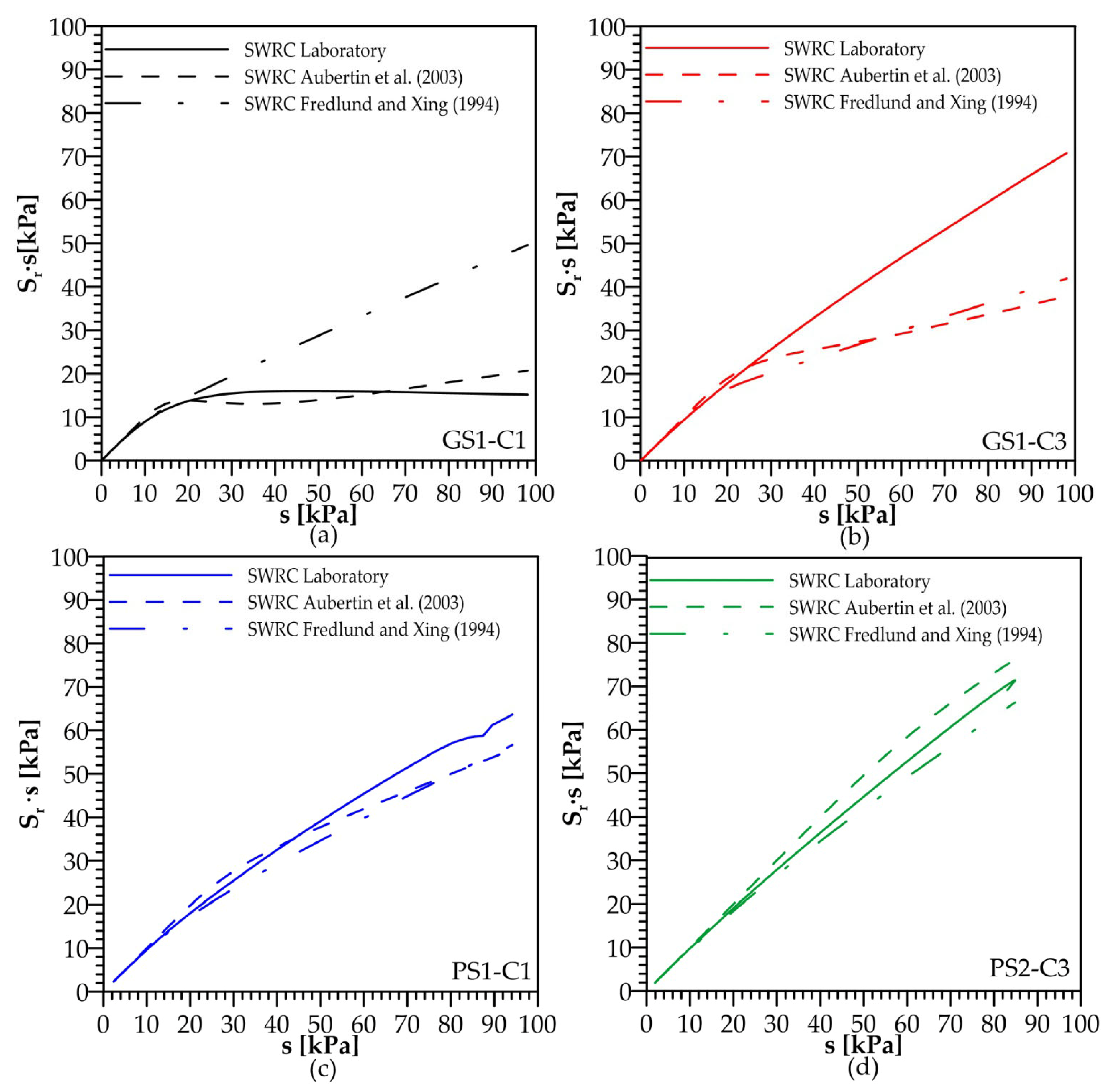
Table A3.
Mechanical parameters of the Tagliamento River soil samples for the determination of SWRCs through the model of Aubertin et al. (2003) [52].
Table A4.
Mechanical parameters of the Tagliamento River soil samples for the determination of SWRCs through the model of Fredlund and Xing (1994) [53].
Appendix B. Sensitivity of the CPT-Based Friction Angle to Matric Suction
The CPT-based correlations proposed in this study account for the contribution of matric suction to the effective stress, as described in Section 2.3. In the adopted Bishop’s effective-stress formulation, the suction contribution depends on the product χ∙s, with χ assumed equal to the degree of saturation, Sr. Consequently, the influence of matric suction on the estimated friction angle, φ′CPT, depends not only on the magnitude of suction but also on the soil–water retention behaviour of the investigated material.
In Equation (8), matric suction is assumed to vary linearly between the groundwater table and the levee crest. This represents a simplified description of the hydraulic conditions within the embankment, whereas actual suction profiles may be affected by infiltration, evaporation, vegetation, and other atmospheric and hydrological processes, particularly in shallow portions of the embankment. Since field measurements of matric suction profiles were not available for the three investigated sites, a sensitivity analysis was performed to quantify the effect of variations in matric suction on the estimate of φ′CPT at shallow depth.
The analysis was carried out using the SWRCs experimentally determined in the laboratory for four representative samples, namely GS1-C1, GS1-C3, PS1-C1, and PS2-C3. For each sample, the corresponding SWRC was used to determine Sr at different matric suction values. The analysis was performed at a reference depth of 1 m for all samples and considered cone tip resistance values, qc, ranging from 2 to 6 MPa. For each selected qc and matric suction value, φ′CPT was calculated using the three CPT normalisation approaches proposed in the study (Equations (15)–(17)).
The results are presented in Figure A2. The four panels correspond to the SWRCs of the investigated samples, while the different curves represent the considered qc values and the three CPT normalisation approaches. For a given qc, the variation in φ′CPT over the investigated suction range [0; 100 kPa] is approximately 4–5° for most of the investigated samples, whereas a smaller variation of approximately 2° is observed for GS1-C1. This indicates that the sensitivity to matric suction depends on the water-retention behaviour of the material.
Since the proposed equations are logarithmic with respect to the effective stress, for the investigated samples, the variation in φ′CPT is generally more pronounced at relatively low suction values and tends to become less pronounced as suction increases.
Figure A2.
Sensitivity of the estimated peak friction angle, (φ′CPT) to matric suction for four investigated soil samples at a reference depth of 1 m, assuming a total vertical stress, (σv), of 19 kPa: (a) GS1-C1; (b) GS1-C3; (c) PS1-C1; and (d) PS2-C3. The curves were obtained using the corresponding laboratory-derived soil–water retention curves, cone tip resistance values ranging from 2 to 6 MPa, and the three CPT normalisation approaches given by Equations (15)–(17).
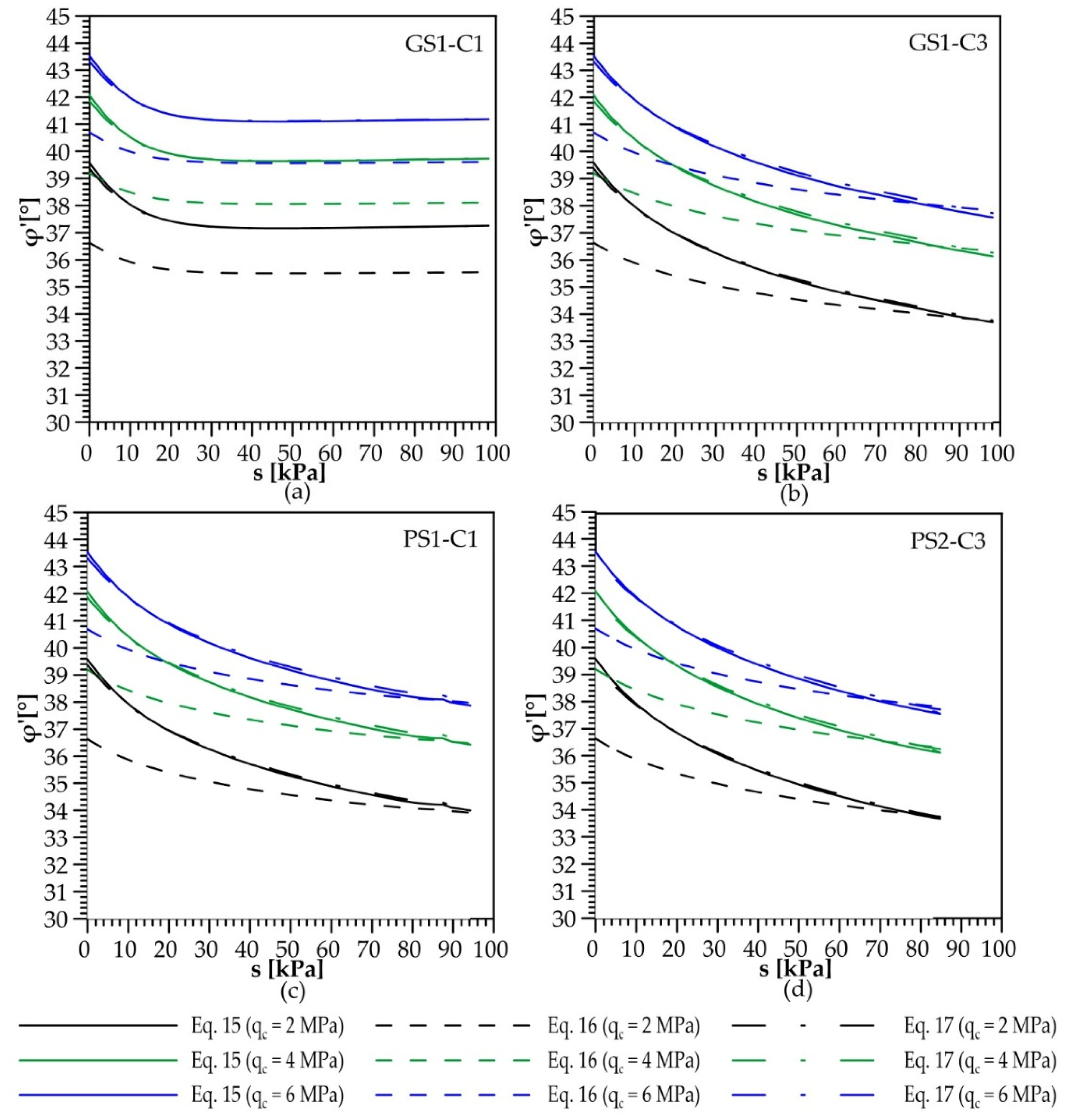
This behaviour is consistent with the non-linear relationship between matric suction and Sr described by the corresponding SWRCs. Under the adopted assumption χ = Sr, the suction contribution to the effective stress is governed by the combined term Sr∙s. Therefore, the same variation in matric suction may result in different changes in φ′CPT depending on the retention behaviour of the soil.
Appendix C. Assessment of the Influence of the Calibration Dataset on the Proposed CPT Correlations
To assess the influence of the inclusion of data obtained from calibration-chamber tests on the proposed CPT correlations, an additional analysis was performed by considering separately the data from the three investigated river sites and the complete dataset used in this study. The analysis was carried out for the three normalisation approaches for cone tip resistance considered in Equations (15)–(17).
Two cases were considered. In Case A, the correlations were calibrated exclusively using the samples collected from the three investigated river sites (n = 26). In Case B, the calibration was performed using the complete dataset, including both the field data and the data obtained from calibration-chamber tests available in the literature. Figure A3, Figure A4 and Figure A5 show the correlations obtained for the three normalisation approaches, while Table A5 and Table A6 report the RMSE and MAE values, respectively, obtained by applying the two formulations to the field data and to the complete dataset.
Figure A3.
Correlation between the laboratory-derived effective friction angle (φ′LAB) and the normalised net cone resistance, [(qc − p0)/p′0] + 1, for Case A (field data only) and Case B (combined field and calibration-chamber data). The logarithmic regression line for Case A is shown in blue, whereas that for Case B is shown as a dashed black line. The corresponding regression equations and R2 values are reported for both cases. For Case A, R2 is calculated using the field dataset only, whereas for Case B, R2 is calculated using the full combined dataset, comprising field data and calibration-chamber data from the literature.
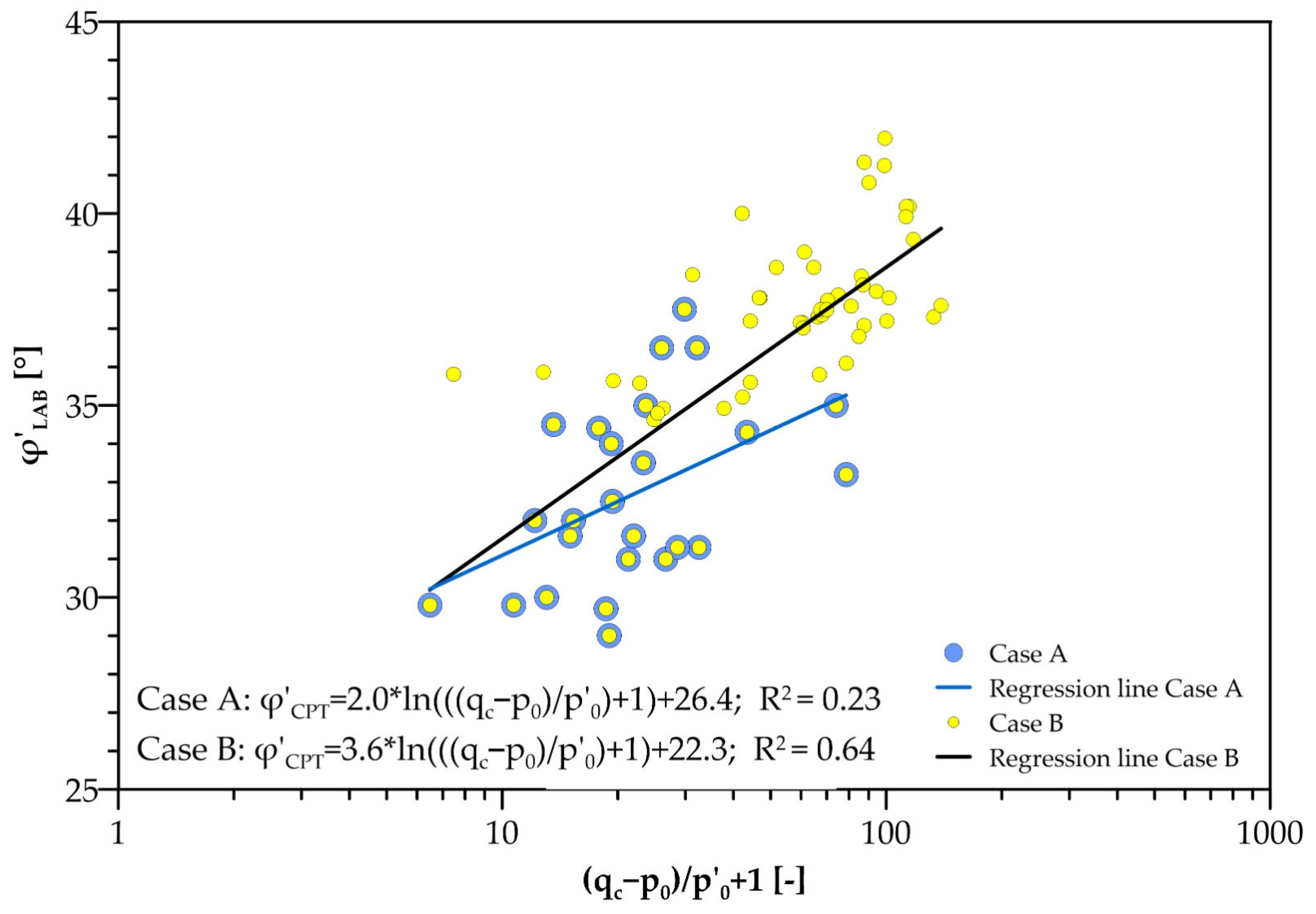
Figure A4.
Correlation between the laboratory-derived effective friction angle (φ′LAB) and the stress-normalised cone tip resistance, (qc/Pa)/(σ′v/Pa)0.5, for Case A (field data only) and Case B (combined field and calibration-chamber data). The logarithmic regression line for Case A is shown in blue, whereas that for Case B is shown as a dashed black line. The corresponding regression equations and R2 values are reported for both cases. For Case A, R2 is calculated using the field dataset only, whereas for Case B, R2 is calculated using the full combined dataset, comprising field data and calibration-chamber data from the literature.
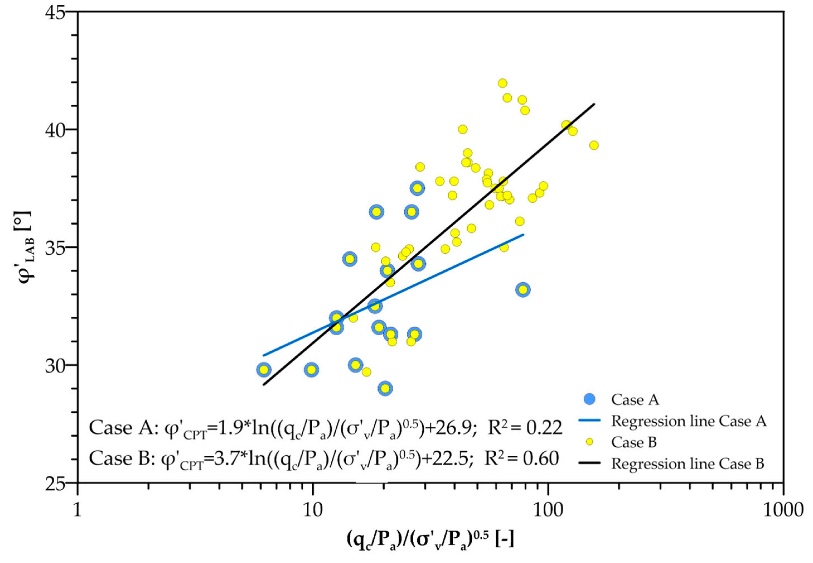
Figure A5.
Correlation between the laboratory-derived effective friction angle (φ′LAB) and the normalised cone tip resistance, qc/σ′v, for Case A (field data only) and Case B (combined field and calibration-chamber data). The logarithmic regression line for Case A is shown in blue, whereas that for Case B is shown as a dashed black line. The corresponding regression equations and R2 values are reported for both cases. For Case A, R2 is calculated using the field dataset only, whereas for Case B, R2 is calculated using the full combined dataset, comprising field data and calibration-chamber data from the literature.
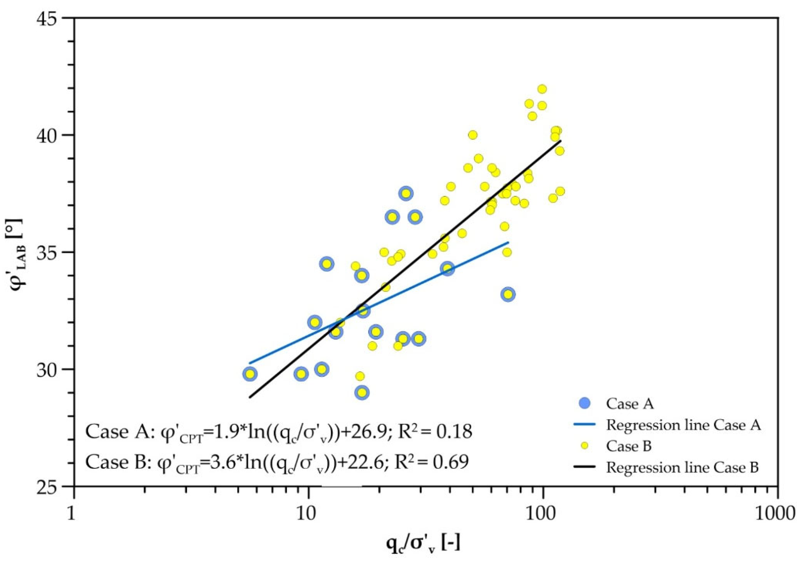
The analysis of Figure A3, Figure A4 and Figure A5 show that the coefficient of determination obtained using only the field data is systematically lower than that obtained from the complete dataset. This difference should be interpreted considering the different distribution of the data in the two datasets. The samples collected from the river embankments cover a relatively narrow range of normalised cone tip resistance and friction angle, whereas the inclusion of the calibration-chamber data extends the range of conditions represented by the regression. Consequently, the regression based exclusively on the field data is determined over a more limited range of variation in the independent variable.
In this context, R2 should be interpreted together with the size and distribution of the dataset. In particular, a restricted range of the independent variable may result in a relatively low R2 even when the absolute prediction errors remain limited, because a larger proportion of the observed variability in the dependent variable is then associated with residual dispersion rather than with variations in the independent variable.
The inclusion of the calibration-chamber data, in contrast, extends the range of normalised cone tip resistance and friction angle represented in the regression. The higher slopes obtained for Case B in Figure A3, Figure A4 and Figure A5 (3.6–3.7, compared with 1.9–2.0 for Case A) may be related to the broader range of normalised cone tip resistance and friction angle represented in the combined dataset.
Table A5 and Table A6 reports the RMSE and the MAE calculated with the regression line of Case A and Case B over the field data and over the entire combined dataset. The comparison of column 2 and 3 quantifies the change in estimation error associated with using the combined-dataset correlation (Case B) instead of the field-only correlation (Case A), by evaluating both correlations against the same field observations. This comparison directly evaluates whether the inclusion of the calibration-chamber data results in a significant loss of accuracy within the main application domain of the study.
For all the normalisation approaches, RMSE and MAE values for Case B calculated over the field test data are only slightly larger than those calculated for Case A.
Table A5.
Comparison of RMSE values for the three CPT normalization approaches. Case A refers to correlations calibrated using only the field data, whereas Case B refers to correlations calibrated using the combined field and calibration-chamber dataset.
Table A6.
Comparison of MAE values [°] for the three CPT normalization approaches. Case A refers to correlations calibrated using only the field data, whereas Case B refers to correlations calibrated using the combined field and calibration-chamber dataset.
The field-data assessment quantifies the trade-off between extending the calibration domain and maintaining agreement with the observations from the investigated levees. Using the combined-data correlation increases the field RMSE by maximum 0.55° and the MAE by 0.31°. Thus, although the regression coefficients change appreciably, the resulting increases in field prediction error are approximately 0.2–0.5°.
These results provide a quantitative basis for retaining the combined calibration for the broader-domain objective of this study. The inclusion of calibration-chamber records extends the range of normalised cone resistance and friction angle represented in the database, while field errors remain of the same order of magnitude as those obtained from the field-only calibration. This choice therefore involves an explicit trade-off: broader calibration coverage is obtained at the cost of a limited reduction in agreement with the field observations.
References
- Robertson, P.K.; Cabal, K.L. Guide to Cone Penetration Testing for Geotechnical Engineering; Gregg Drilling & Testing: Signal Hill, CA, USA, 2015. [Google Scholar]
- Lunne, T.; Berre, T.; Strandvik, S. Sample disturbance effects in soft low-plastic Norwegian clay. In Proceedings of the Symposium on Recent Developments in Soil and Pavement Mechanics, Rio de Janeiro, Brazil, 25–27 June 1997. [Google Scholar]
- Cami, B.; Javankhoshdel, S.; Phoon, K.K.; Ching, J. Scale of fluctuation for spatially varying soils: Estimation methods and values. ASCE-ASME J. Risk Uncertain. Eng. Syst. Part A Civ. Eng. 2020, 6, 03120002. [Google Scholar] [CrossRef] [Scilit]
- Ceccato, F.; Uzielli, M.; Simonini, P. Characterization of geotechnical spatial variability in river embankments from spatially adjacent SCPT. In Cone Penetration Testing 2022; CRC Press: Boca Raton, FL, USA, 2022; pp. 863–869. [Google Scholar]
- Dalla Santa, G.; Ceccato, F.; Simonini, P. Geotechnical characterization of the levees of the Tagliamento River (Italy): Insights and implications for levee vulnerability. In Proceedings of the 9th International Symposium on Geotechnical Safety and Risk (ISGSR); Research Publishing: Singapore, 25–28 August 2025. [Google Scholar]
- Fredlund, D.G.; Rahardjo, H. An overview of unsaturated soil behaviour. Geotech. Spec. Publ. 1993, 39, 1–35. [Google Scholar]
- Fredlund, D.G.; Vanapalli, S.K.; Xing, A.; Pufahl, D.E. Predicting the shear strength function for unsaturated soils using the soil-water characteristic curve. In Proceedings of the 1st International Conference on Unsaturated Soils, Paris, France, 6–8 September 1995; Volume 1, pp. 63–69. [Google Scholar]
- Vanapalli, S.K.; Fredlund, D.G.; Pufahl, D.E.; Clifton, A.W. Model for the prediction of shear strength with respect to soil suction. Can. Geotech. J. 1996, 33, 379–392. [Google Scholar] [CrossRef] [Scilit]
- Ceccato, F.; Dalla Santa, G.; Simonini, P. Challenges in interpreting CPT for river levee material characterization. In Proceedings of the 9th International Symposium on Geotechnical Safety and Risk (ISGSR), Oslo, Norway, 25–28 August 2025. [Google Scholar]
- Tang, C.T.; Borden, R.H.; Gabr, M.A. Approach for estimating effective friction angle from cone penetration test in unsaturated residual soils. J. Geotech. Geoenviron. Eng. 2017, 143, 04017087. [Google Scholar] [CrossRef] [Scilit]
- Giacheti, H.L.; Bezerra, R.C.; Rocha, B.P.; Rodrigues, R.A. Seasonal influence on cone penetration test: An unsaturated soil site example. J. Rock Mech. Geotech. Eng. 2019, 11, 361–368. [Google Scholar] [CrossRef] [Scilit]
- Jommi, C.; Muraro, S.; Chao, C. Interpreting repeated CPT in unsaturated soils. In Proceedings of the 7th International Conference on Geotechnical and Geophysical Site Characterization (ISC’7), Barcelona, Spain, 18–21 June 2024; pp. 566–573. [Google Scholar]
- Lehane, B.M.; Ismail, M.A.; Fahey, M. Seasonal dependence of in situ test parameters in sand above the water table. Géotechnique 2004, 54, 215–218. [Google Scholar] [CrossRef]
- Houston, S.; Houston, W.N.; Anderson, T.W. Moisture and strength variability in some Arizona subgrades. Transp. Res. Rec. 1995, 1481, 35–43. [Google Scholar]
- Lo Presti, D.; Stacul, S.; Meisina, C.; Bordoni, M.; Bittelli, M. Preliminary validation of a novel method for the assessment of effective stress state in partially saturated soils by cone penetration tests. Geosciences 2018, 8, 30. [Google Scholar] [CrossRef] [Scilit]
- Russell, A.R.; Vo, T.; Ayala, J.; Wang, Y.; Reid, D.; Fourie, A.B. Cone penetration tests in saturated and unsaturated silty tailings. Géotechnique 2024, 74, 281–295. [Google Scholar] [CrossRef] [Scilit]
- Russell, A.R. Water retention characteristics of soils with double porosity. Eur. J. Soil Sci. 2010, 61, 412–424. [Google Scholar] [CrossRef] [Scilit]
- Pournaghiazar, M.; Russell, A.R.; Khalili, N. The cone penetration test in unsaturated sands. Géotechnique 2013, 63, 1209–1220. [Google Scholar] [CrossRef] [Scilit]
- Miller, G.A.; Tan, N.K.; Collins, R.W.; Muraleetharan, K.K. Cone penetration testing in unsaturated soils. Transp. Geotech. 2018, 17, 85–99. [Google Scholar] [CrossRef] [Scilit]
- Keshmiri, E.; Ahmadi, M.M. Interpretation of CPT in unsaturated sands under drained conditions: A numerical study. Int. J. Numer. Anal. Methods Geomech. 2021, 45, 2732–2755. [Google Scholar] [CrossRef] [Scilit]
- Yang, H.; Russell, A.R. Cone penetration tests in unsaturated silty sands. Can. Geotech. J. 2015, 53, 431–444. [Google Scholar] [CrossRef] [Scilit]
- Russell, A.R.; Khalili, N. A unified bounding surface plasticity model for unsaturated soils. Int. J. Numer. Anal. Methods Geomech. 2006, 30, 181–212. [Google Scholar] [CrossRef] [Scilit]
- Robertson, P.K.; Campanella, R.G. Interpretation of cone penetration tests. Part I: Sand. Can. Geotech. J. 1983, 20, 718–733. [Google Scholar] [CrossRef] [Scilit]
- Kulhawy, F.H.; Mayne, P.W. Manual on Estimating Soil Properties for Foundation Design; Report EPRI EL-6800; Electric Power Research Institute: Palo Alto, CA, USA, 1990. [Google Scholar]
- Chen, J.W.; Juang, C.H. Determination of drained friction angle of sands from CPT. J. Geotech. Eng. 1996, 122, 374–381. [Google Scholar] [CrossRef] [Scilit]
- Durgunoglu, H.T.; Mitchell, J.K. Static penetration resistance of soils: I—Analysis. In In Situ Measurement of Soil Properties; ASCE: Reston, VA, USA, 1975; pp. 151–171. [Google Scholar]
- ASTM D6467-21E01; Standard Test Method for Torsional Ring Shear Test to Determine Drained Residual Shear Strength of Fine-Grained Soils. ASTM International: West Conshohocken, PA, USA, 2021.
- ISO 17892-9:2018; Geotechnical Investigation and Testing—Laboratory Testing of Soil—Part 9: Consolidated Triaxial Compression Tests on Water-Saturated Soils. ISO: Geneva, Switzerland, 2018.
- ISO 17892-10:2018; Geotechnical Investigation and Testing—Laboratory Testing of Soil—Part 10: Direct Shear Tests. ISO: Geneva, Switzerland, 2018.
- Castellanos, B.A.; Brandon, T.L. A comparison between the shear strength measured with direct shear and triaxial devices on undisturbed and remolded soils. In Proceedings of the 18th International Conference on Soil Mechanics and Geotechnical Engineering, Paris, France, 2–6 September 2013; Volume 1, pp. 317–320. [Google Scholar]
- Lini Dev, K.; Pillai, R.J.; Robinson, R.G. Drained angle of internal friction from direct shear and triaxial compression tests. Int. J. Geotech. Eng. 2016, 10, 283–287. [Google Scholar] [CrossRef] [Scilit]
- Stefanow, D.; Dudziński, P.A. Soil shear strength determination methods—State of the art. Soil Tillage Res. 2021, 208, 104881. [Google Scholar] [CrossRef] [Scilit]
- Öberg, A.-L.; Sällfors, G. Determination of shear strength parameters of unsaturated silts and sands based on the water retention curve. Geotech. Test. J. 1997, 20, 40–48. [Google Scholar] [CrossRef] [Scilit]
- Schrefler, B.A. The Finite Element method in Soil Consolidation (with Applications to Surface Subsidence). Doctoral Dissertation, University College of Swansea, Swansea, UK, 1984. [Google Scholar]
- Jommi, C. Remarks on the constitutive modelling of unsaturated soils. In Experimental Evidence and Theoretical Approaches in Unsaturated Soils; Tarantino, A., Mancuso, C., Eds.; Balkema: Rotterdam, The Netherlands, 2000; pp. 139–153. [Google Scholar]
- Sheng, D.; Smith, D.W.; Sloan, S.W.; Gens, A. Finite element formulation and algorithms for unsaturated soils. Part II: Verification and application. Int. J. Numer. Anal. Methods Geomech. 2003, 27, 767–790. [Google Scholar] [CrossRef] [Scilit]
- Nuth, M.; Laloui, L. Effective stress concept in unsaturated soils: Clarification and validation of a unified framework. Int. J. Numer. Anal. Methods Geomech. 2008, 32, 771–801. [Google Scholar] [CrossRef] [Scilit]
- Capotosto, A.; Russo, G. Yielding and critical state behaviour of a lime stabilized compacted alluvial soil. In Deformation Characteristics of Geomaterials; IOS Press: Amsterdam, The Netherlands, 2011; pp. 738–745. [Google Scholar]
- Geiser, F.; Laloui, L.; Vulliet, L. Elasto-plasticity of unsaturated soils: Laboratory test results on a remoulded silt. Soils Found. 2006, 46, 545–556. [Google Scholar] [CrossRef] [Scilit]
- Thu, T.M.; Rahardjo, H.; Leong, E.C. Critical state behavior of a compacted silt specimen. Soils Found. 2007, 47, 749–755. [Google Scholar] [CrossRef] [Scilit]
- Sheng, D.; Zhou, A.; Fredlund, D.G. Shear strength criteria for unsaturated soils. Geotech. Geol. Eng. 2011, 29, 145–159. [Google Scholar] [CrossRef] [Scilit]
- Rotisciani, G.M.; Desideri, A.; Amorosi, A. Unsaturated structured soils: Constitutive modelling and stability analyses. Acta Geotech. 2021, 16, 3355–3380. [Google Scholar] [CrossRef] [Scilit]
- Thu, T.M.; Rahardjo, H.; Leong, E.C. Shear strength and pore-water pressure characteristics during constant water content triaxial tests. J. Geotech. Geoenviron. Eng. 2006, 132, 411–419. [Google Scholar] [CrossRef] [Scilit]
- Cattoni, E.; Cecconi, M.; Pane, V. Geotechnical properties of an unsaturated pyroclastic soil from Roma. Bull. Eng. Geol. Environ. 2007, 66, 403–414. [Google Scholar] [CrossRef] [Scilit]
- Gottardi, G.; Gragnano, C.G.; Rocchi, I.; Bittelli, M. Assessing river embankment stability under transient seepage conditions. Procedia Eng. 2016, 158, 350–355. [Google Scholar] [CrossRef] [Scilit]
- Rocchi, I.; Gragnano, C.G.; Govoni, L.; Bittelli, M.; Gottardi, G. Assessing the performance of a versatile and affordable geotechnical monitoring system for river embankments. Phys. Chem. Earth 2020, 117, 102872. [Google Scholar] [CrossRef] [Scilit]
- Gragnano, C.G.; Rocchi, I.; Gottardi, G. Field monitoring and laboratory testing for an integrated modeling of river embankments under transient conditions. J. Geotech. Geoenviron. Eng. 2021, 147, 05021006. [Google Scholar] [CrossRef] [Scilit]
- Ceccato, F.; Dalla Santa, G.; Pacella, G.; Simonini, P. Thermo-hydraulic monitoring and modelling of the Grizzaga river levee. In Proceedings of the IX Convegno Nazionale Dei Ricercatori Di Ingegneria Geotecnica (CNRIG 2026), L’Aquila, Italy, 1–3 June 2026. [Google Scholar]
- D’Alessio, G.; Lalicata, L.M.; Casini, F. Hydro–mechanical analysis of embankments stability in partially saturated soils under rainfall events. E3S Web Conf. 2025, 642, 02022. [Google Scholar]
- Dane, J.H.; Topp, G.C. (Eds.) Methods of Soil Analysis. Part 4: Physical Methods; John Wiley & Sons: Hoboken, NJ, USA, 2020. [Google Scholar]
- Solone, R.; Bittelli, M.; Tomei, F.; Morari, F. Errors in water retention curves determined with pressure plates: Effects on the soil water balance. J. Hydrol. 2012, 470–471, 65–74. [Google Scholar] [CrossRef] [Scilit]
- Aubertin, M.; Mbonimpa, M.; Bussière, B.; Chapuis, R.P. A model to predict the water retention curve from basic geotechnical properties. Can. Geotech. J. 2003, 40, 1104–1122. [Google Scholar] [CrossRef] [Scilit]
- Fredlund, D.G.; Xing, A. Equations for the soil-water characteristic curve. Can. Geotech. J. 1994, 31, 521–532. [Google Scholar] [CrossRef] [Scilit]
- Kovács, G. Seepage Hydraulics; Developments in Water Science; Elsevier: Amsterdam, The Netherlands, 1981; Volume 10. [Google Scholar]
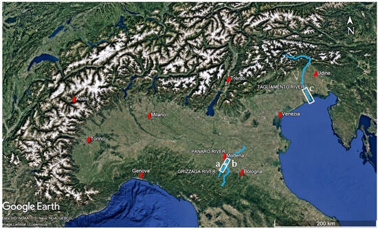
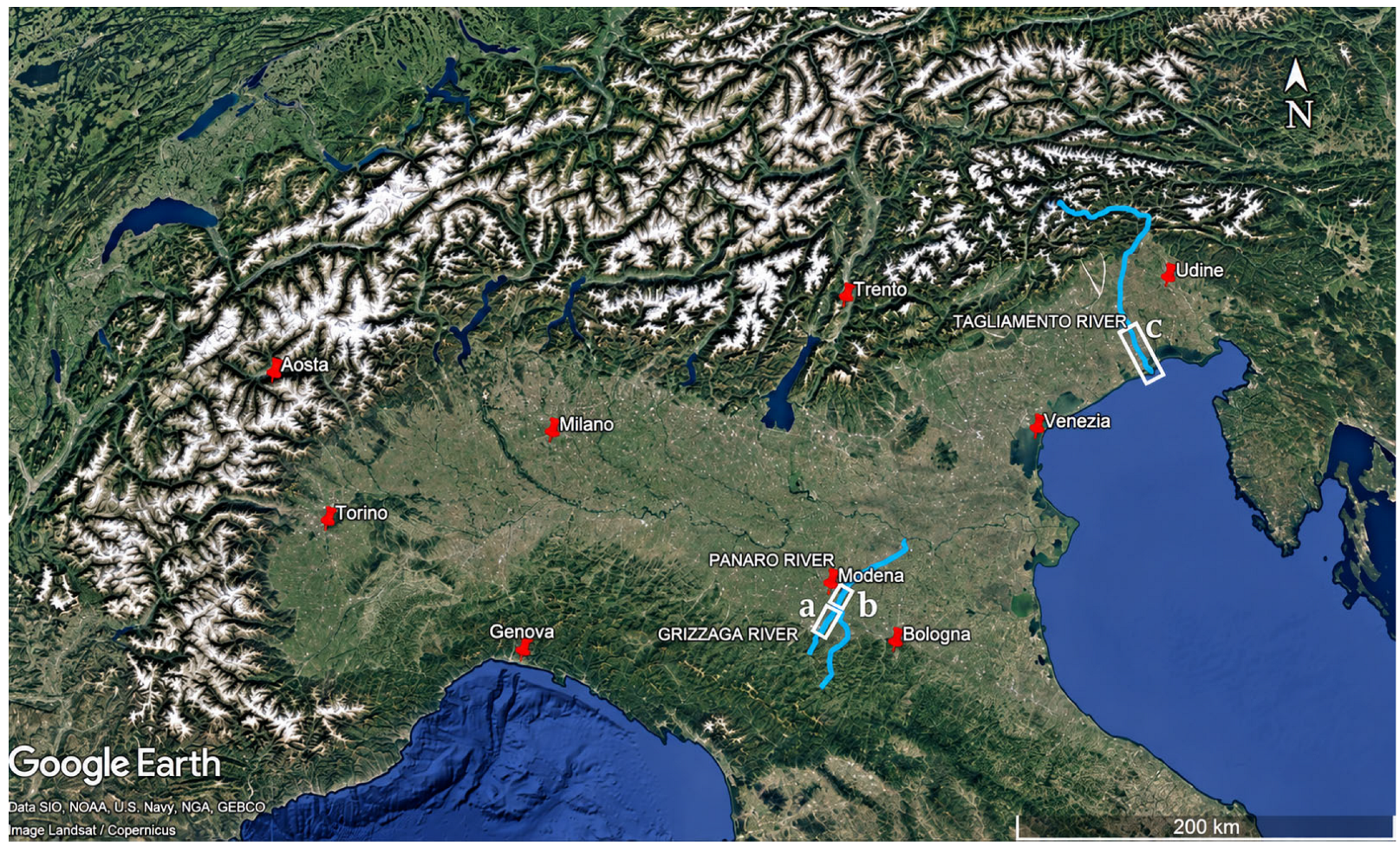
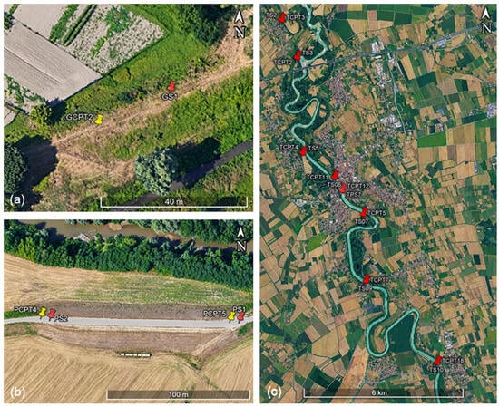
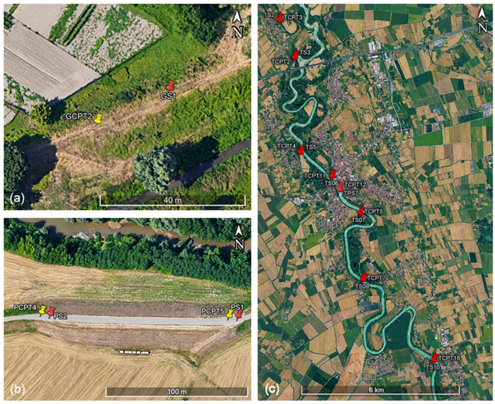
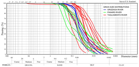
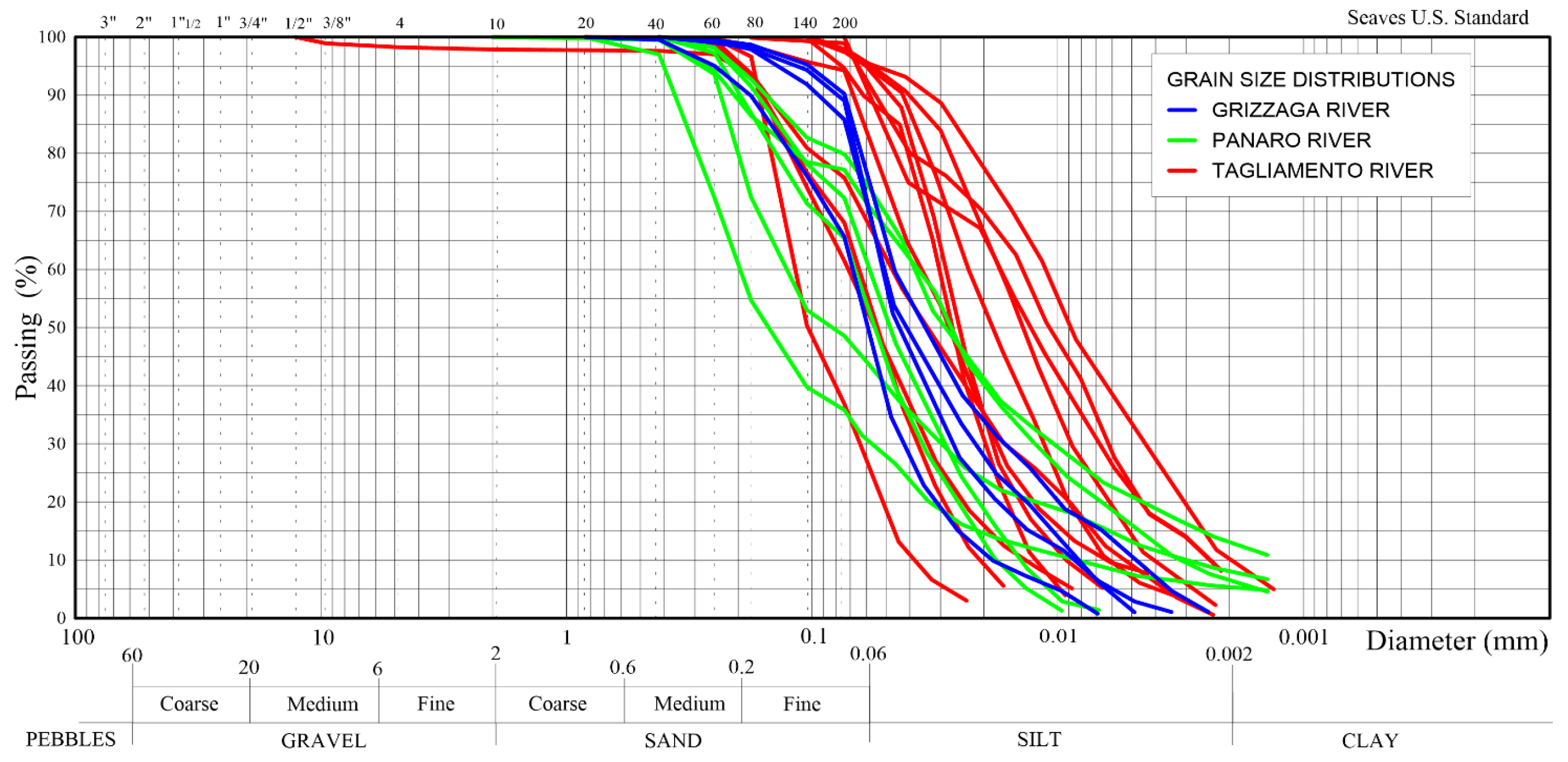
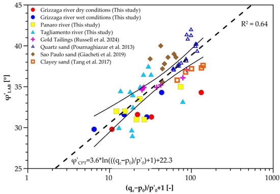
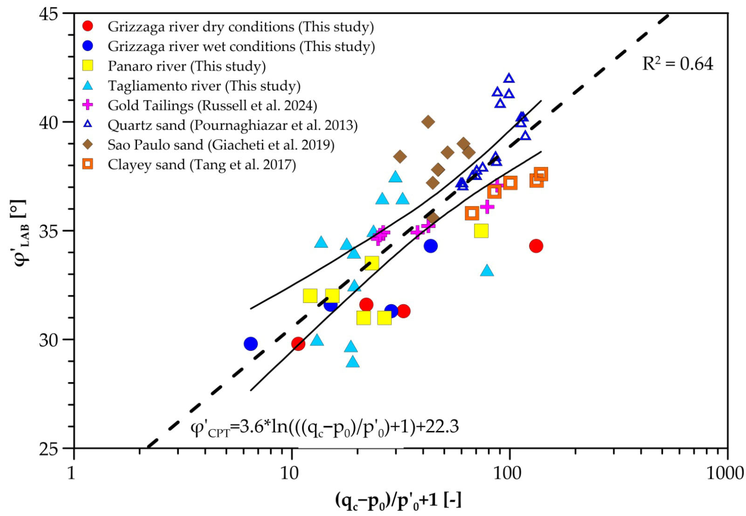
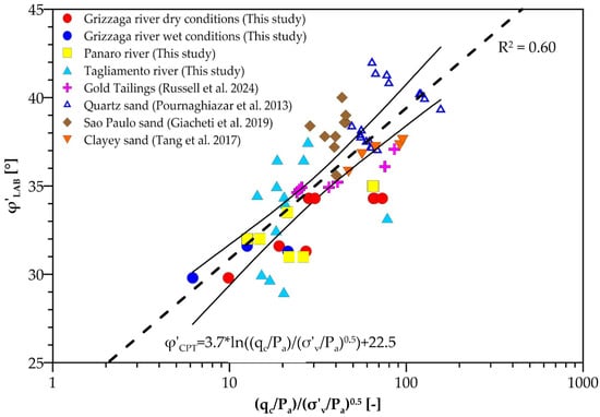
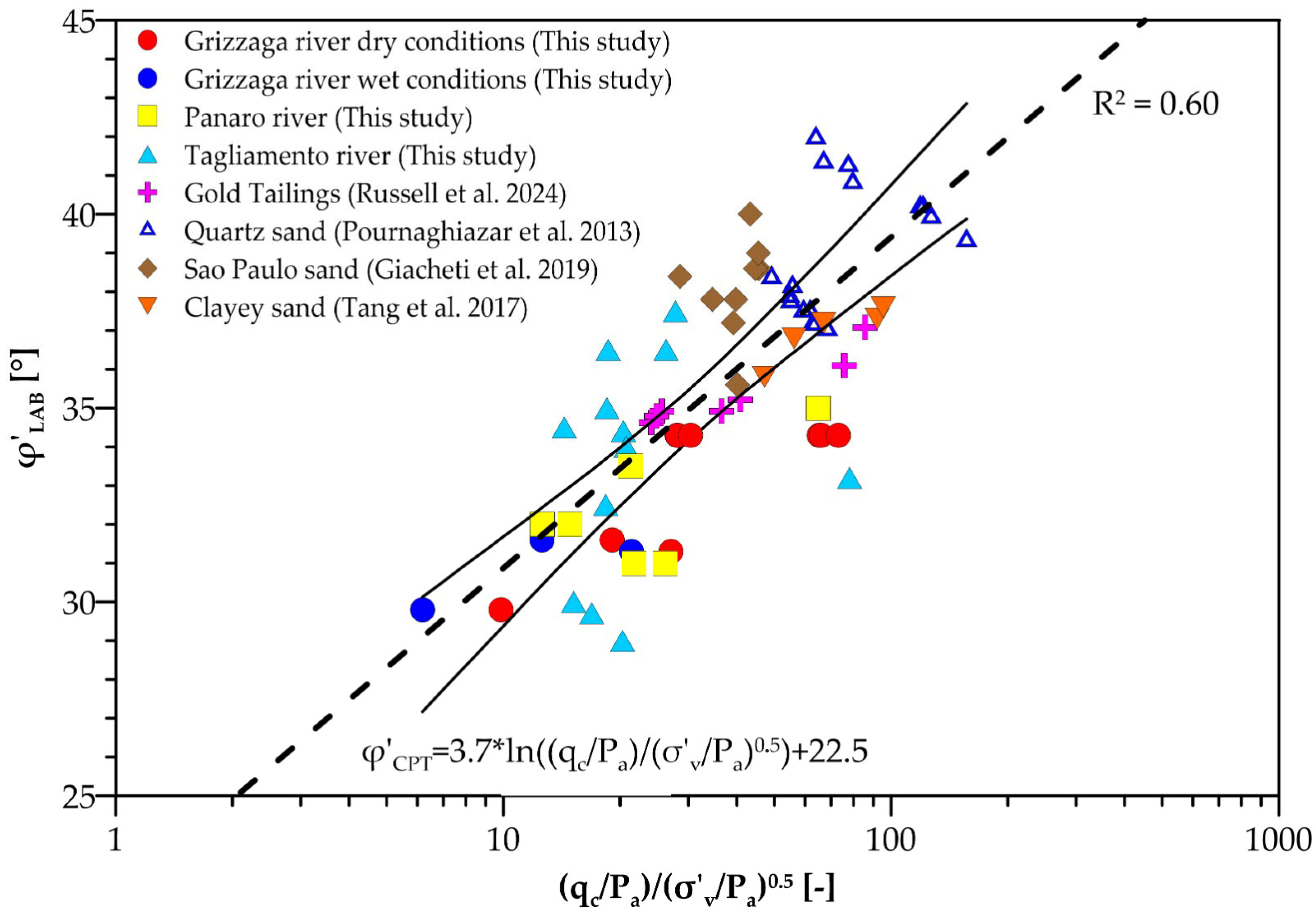
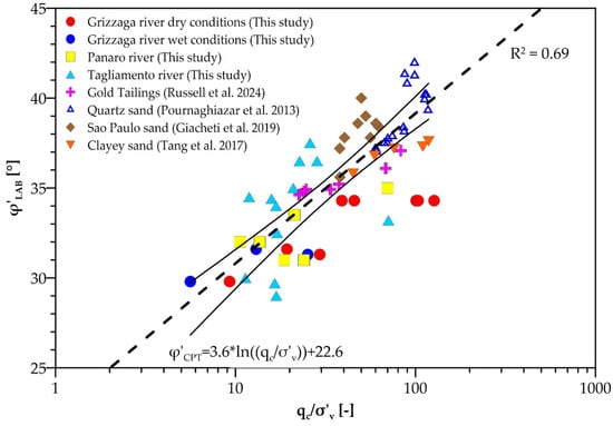
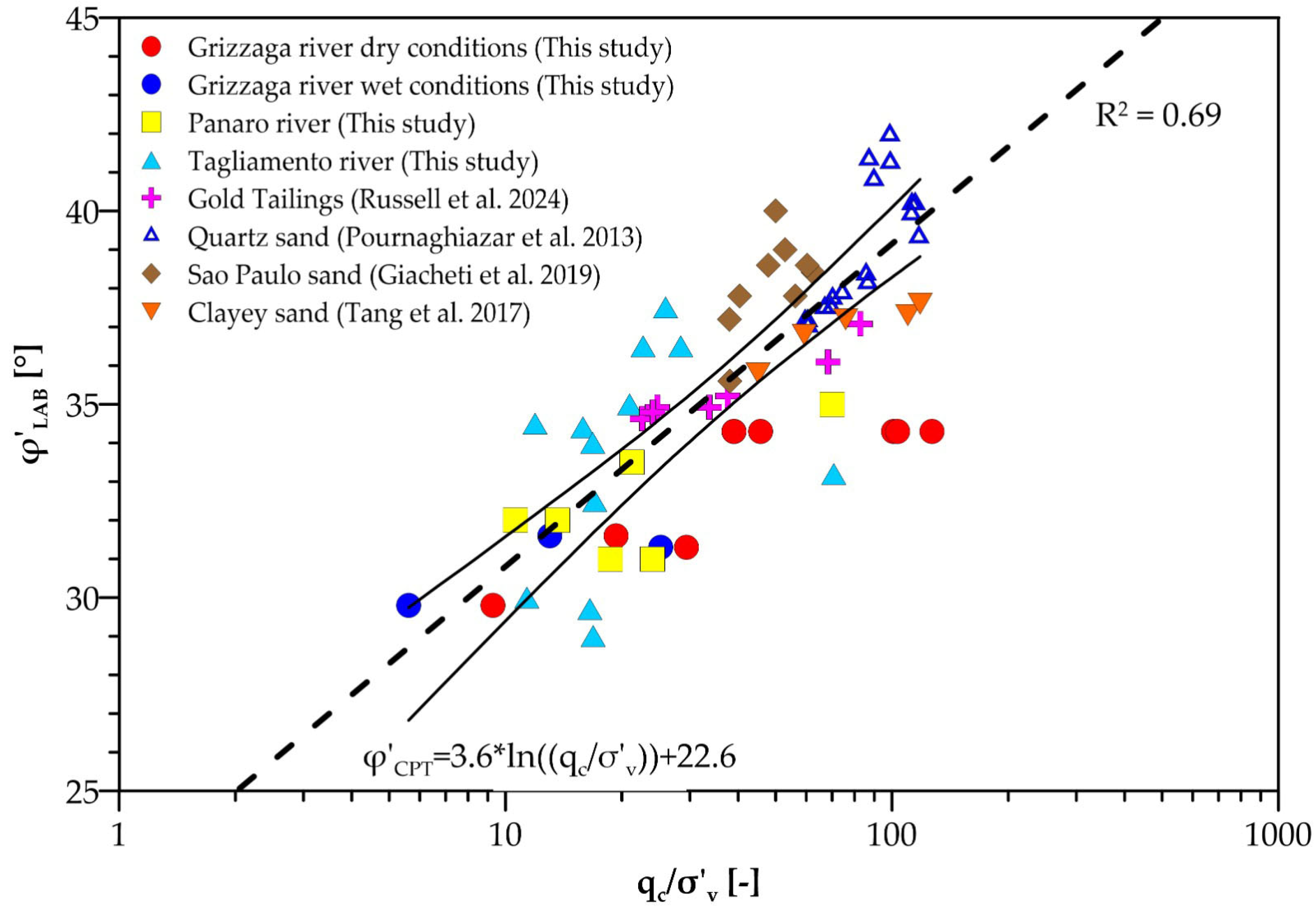
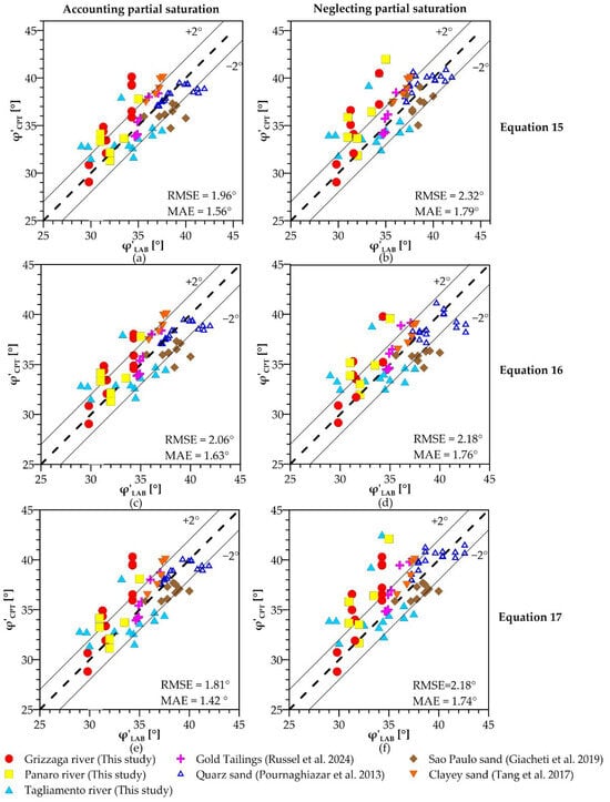
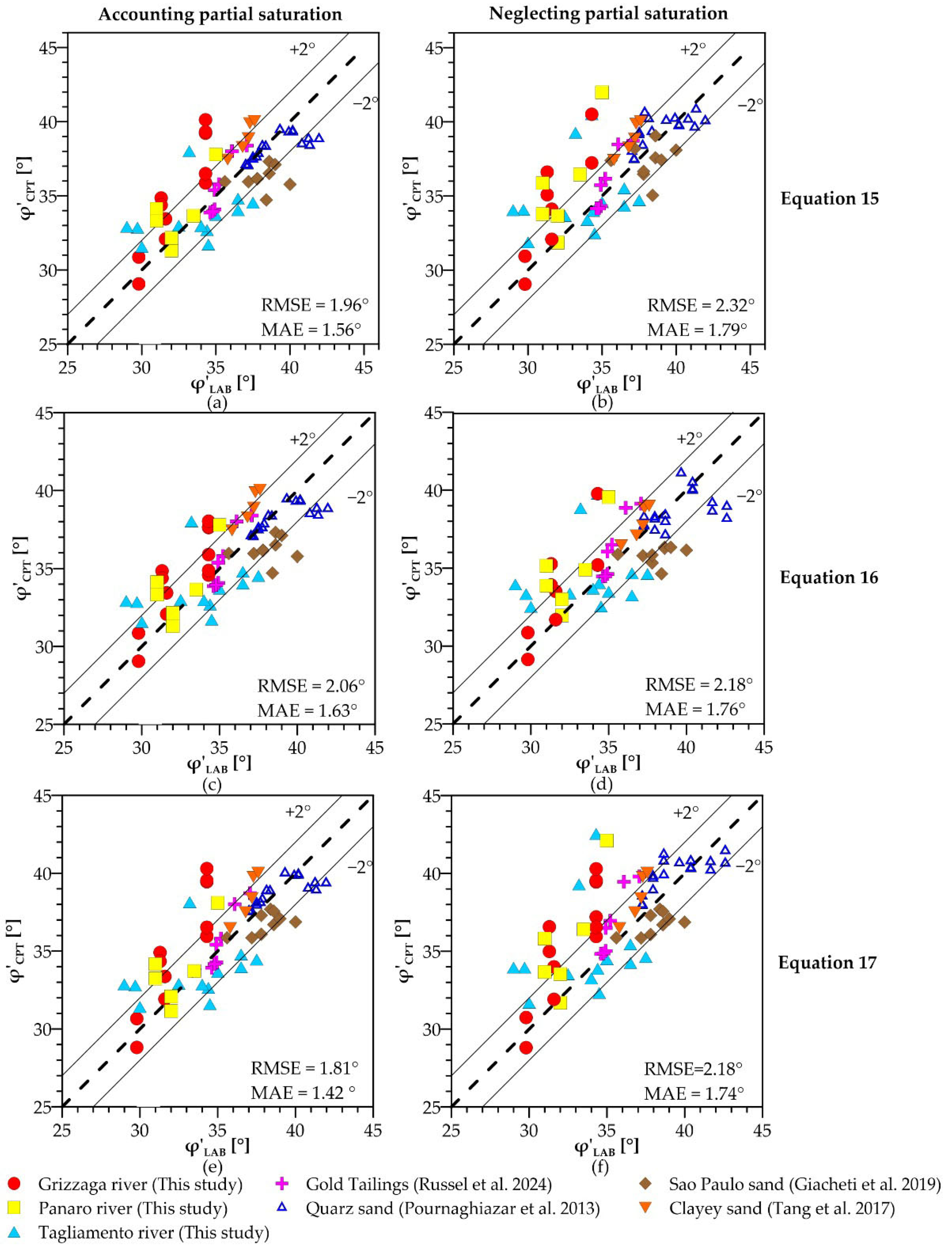
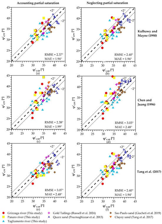
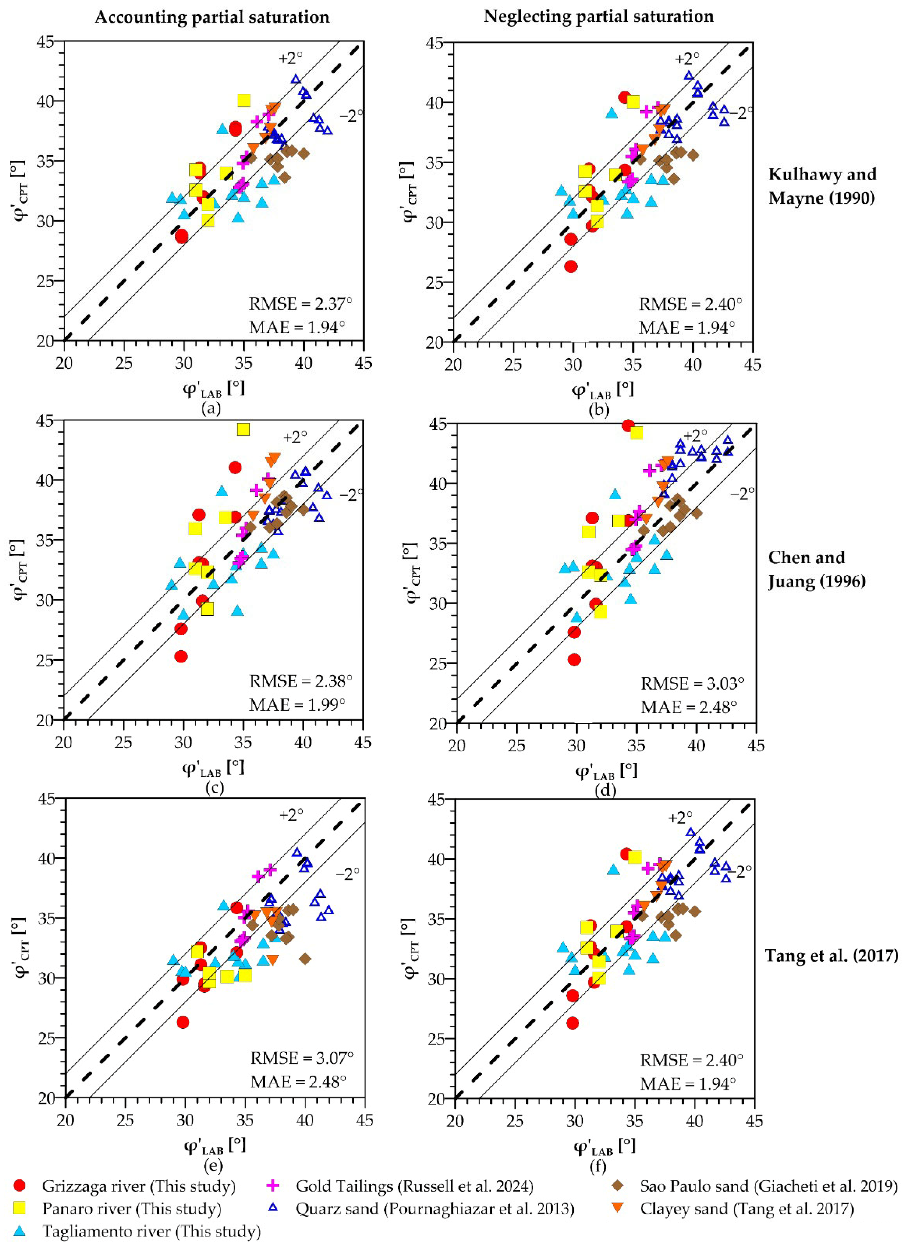
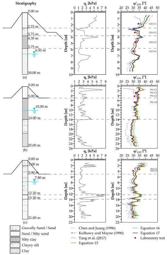
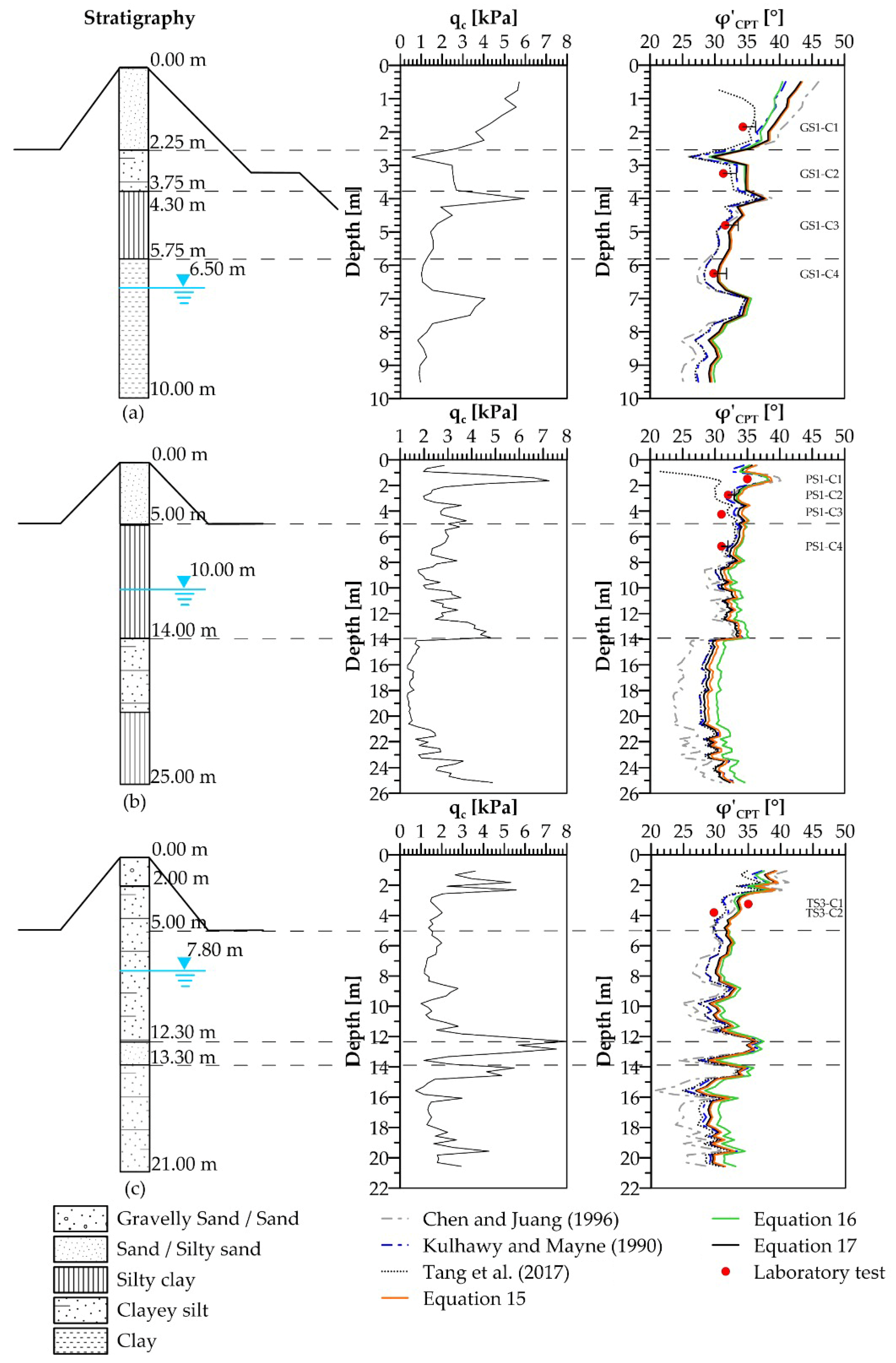

Disclaimer/Publisher’s Note: The statements, opinions and data contained in all publications are solely those of the individual author(s) and contributor(s) and not of MDPI and/or the editor(s). MDPI and/or the editor(s) disclaim responsibility for any injury to people or property resulting from any ideas, methods, instructions or products referred to in the content. |
© 2026 by the authors. Licensee MDPI, Basel, Switzerland. This article is an open access article distributed under the terms and conditions of the Creative Commons Attribution (CC BY) license.