


Abstract
The accuracy of discrete element method (DEM) simulations depends on the appropriate selection of microscopic parameters. However, conventional calibration using biaxial tests requires repeated adjustment of microscopic parameters until the macroscopic responses of numerical specimens match the target responses, making the process cumbersome and computationally demanding. In this regard, this study presents an interpretable, surrogate-assisted machine-learning framework for analyzing and calibrating DEM parameters of brittle rock materials represented by the Hertz–Mindlin bonded contact model. Decision tree (DT), random forest (RF), and eXtreme Gradient Boosting (XGBoost) were selected to compare single-tree and ensemble-tree regression approaches for capturing the nonlinear relationships between three microscopic parameters—friction coefficient μ, bond tensile strength Tb, and bond cohesion Cb—and two macroscopic parameters, bulk cohesion Co and internal friction angle φ. SHapley Additive exPlanations (SHAP) was subsequently employed to quantify and interpret the contributions of individual microscopic parameters. XGBoost showed the best performance for predicting the macroscopic parameters, whereas Tb was less reliably predicted than μ and Cb. SHAP indicated that Cb and Tb contributed most strongly to Co, while μ dominated φ. Finally, differential evolution (DE) was combined with the forward prediction model to search for feasible microscopic parameter combinations reproducing prescribed macroscopic responses.
1. Introduction
The discrete element method (DEM), originally introduced by Cundall and Strack [1,2], simulates the mechanical behavior of granular materials by representing them as a series of discrete cells and describing particle motion using Newton’s second law together with an appropriate contact model. DEM can effectively capture the heterogeneous characteristics of geomaterials [3] and has become an important numerical simulation method in geotechnical engineering [4,5,6,7]. However, appropriate calibration of microscopic parameters is essential for obtaining reliable DEM simulation results. Conventional calibration is still primarily conducted through empirical and iterative parameter adjustment, a procedure commonly referred to as the trial-and-error method [8,9]. For example, Zhou et al. [10] used repeated biaxial simulations to examine how variations in microscopic parameters affect the resulting macroscopic behavior of soil specimens. Cheng et al. [11] similarly calibrated DEM microscopic parameters for quartz sand using triaxial tests. More recently, automatic optimization approaches have been introduced to reduce dependence on manual adjustment. Shang et al. [12] developed an intelligent optimization method for heterogeneous rock DEM parameters, while Fan et al. [13] employed an ant colony optimization algorithm for automatic DEM microparameter calibration.
In recent years, machine-learning methods have been introduced into DEM calibration because they can approximate complex and nonlinear mappings between microscopic model inputs and macroscopic mechanical responses. Zhou et al. [14] established a BP neural network for nonlinear macro–micro parameter mapping, while Benvenuti et al. [15] employed an artificial neural network to predict DEM contact-law parameters. Zhou et al. [9] subsequently developed an XGBoost model for macroscopic parameter prediction and microscopic parameter inversion, and Shentu and Lin [3] proposed an end-to-end machine-learning framework for efficient DEM calibration. More recently, Jiang et al. [16] developed a Stacking ensemble-learning model for microscopic-parameter calibration and demonstrated substantial differences in prediction performance among individual microscopic parameters. Zhang et al. [17] further combined an XGBoost-based surrogate model, SHAP analysis, and multi-objective optimization for concrete DEM microparameter calibration.
Although machine learning can effectively approximate nonlinear macro–micro relationships, directly predicting microscopic parameters from macroscopic properties remains challenging because macroscopic responses are generated by combinations of microscopic parameters [3]. Prediction accuracy alone also does not provide a physical explanation of how individual microscopic parameters contribute to macroscopic responses. Conventional control-variable analyses can identify parameter trends, but generally require repeated numerical simulations and provide limited information on parameter contributions over a multidimensional parameter space. Explainable machine-learning techniques have therefore begun to be incorporated into DEM calibration. Zhang et al. [17] combined an XGBoost-based surrogate model with SHAP analysis and multi-objective optimization, while Peng et al. [18] employed SHAP and related interpretation methods within a rigorously validated machine-learning framework. Nevertheless, several issues remain insufficiently addressed. Model-derived sensitivities require further interpretation in terms of the underlying DEM mechanical mechanisms. Moreover, different microscopic parameters may exhibit substantially different levels of predictability, raising questions regarding their identifiability under the selected macroscopic constraints. When a limited number of macroscopic responses are used to constrain multiple microscopic parameters, the reliability and uniqueness of the inverse solution therefore require careful assessment.
Therefore, this study aims to develop an interpretable DEM calibration framework while examining the reliability of microscopic-parameter identification from limited macroscopic responses. Biaxial compression tests based on the Hertz–Mindlin bonded contact model were conducted to investigate the relationships between three microscopic parameters—the friction coefficient μ, bond tensile strength Tb, and bond cohesion Cb—and two macroscopic parameters, bulk cohesion Co and internal friction angle φ, DT, RF, and XGBoost were evaluated for both forward macroscopic prediction and direct microscopic prediction. SHAP was then employed to interpret the contributions of microscopic parameters to macroscopic responses. Finally, the best-performing forward prediction model was coupled with differential evolution to search for microscopic parameter combinations reproducing the prescribed macroscopic responses.
2. Numerical Models and Methods
2.1. Hertz-Mindlin Contact Model
The numerical simulations employ a Hertz–Mindlin contact formulation combined with bonded contacts to represent the mechanical behavior of brittle rock. The bonded formulation allows neighboring particles to transmit tensile and cohesive forces and therefore provides a means of reproducing crack initiation and subsequent propagation [19]. Depending on the loading state, the interaction between two bonded particles is treated differently. Under compression, the contact forces follow the Hertz–Mindlin contact formulation, whereas tensile loading is governed by the bond contact mechanics model [20]. Accordingly, the contact stiffnesses Kn and Ks depend on the corresponding contact state. Generally, the normal and tangential contact forces, denoted by Fn and Fs, respectively, are calculated as follows:
where Kn and Ks denote the normal and tangential contact stiffnesses, respectively, and Un and Us represent the normal relative displacement and the amount of shear overlap between particles, respectively. Within the Hertz-Mindlin contact model, the stiffnesses are nonlinear and depend on the contact geometry and the elastic properties, including the contact area of overlapping particles S, the particle shear modulus G, and Poisson’s ratio v [20,21,22,23,24].
2.2. Machine Learning Models
2.2.1. Extreme Gradient Boosting
XGBoost is an enhanced ensemble learning method based on gradient-boosted decision trees (GBDT) [25,26]. It utilizes a second-order Taylor expansion of the GBDT loss function and incorporates regularization terms. The core idea is to construct a higher-accuracy prediction model by combining multiple weak prediction models through continuous iterations of the gradient boosting technique. Each iteration analyzes and adjusts the predictions from the previous iteration, then it is trained again to improve the accuracy of the model. It is capable of processing large volumes of data within a relatively short period and effectively handling incomplete datasets. In recent years, XGBoost has achieved recorded success in regression tasks [27,28,29]. So, the principle is as follows [25,30].
For a dataset containing n samples, the input–output pairs can be written as
where xi denotes the input vector; yi represents the corresponding target value. Therefore, the model aims to establish the mapping relationship between the input xi and the output yi, as presented in Equation (4).
where represents the model-predicted value; K denotes the number of decision trees; fk represents the weak learner generated using the decision tree (DT) method; and F denotes the functional space consisting of all decision trees. In XGBoost, the objective function can be expressed as follows.
in which l represents realistic training loss between real and predicted values; Ω denotes the complexity of the model. The loss function and model complexity are expressed using Equations (6) and (7). Where γ represents the penalty factor associated with model complexity; T denotes the number of leaf nodes; λ represents the penalty coefficients; and w represents the weight of leaf nodes. During the training iterations of the model, the objective is to minimize the objective function, thereby reducing the discrepancy between the true and predicted values. Therefore, minimizing the objective function using incremental training, add ft in the t-th iteration to update the loss function as follows:
By applying the second-order Taylor expansion to Equation (8), the optimal solution and the corresponding optimal objective function value can be obtained.
2.2.2. Decision Tree
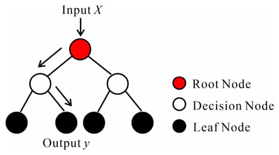
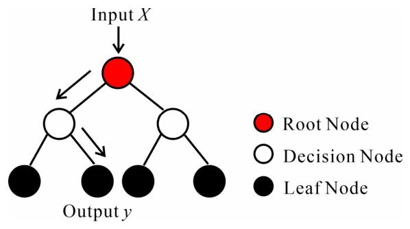
Decision Tree (DT) is a widely used machine learning algorithm that has been widely applied in various fields [31,32,33,34,35]. Figure 1 presents the schematic diagram of the DT model. Its principle is simple: it recursively splits the dataset into smaller subsets by selecting optimal features. This process constructs a series of decision nodes and leaf nodes for data prediction, typically represented as a binary tree structure. At each node, a feature-based rule partitions the data into subsequent branches. The partitioning process continues until the stopping criterion is reached, after which the terminal nodes provide the final predictions.
Figure 1.
Schematic diagram of the DT model. The arrows indicate the direction of data partitioning from parent nodes to child nodes.
2.2.3. Random Forest
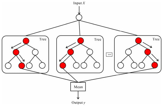
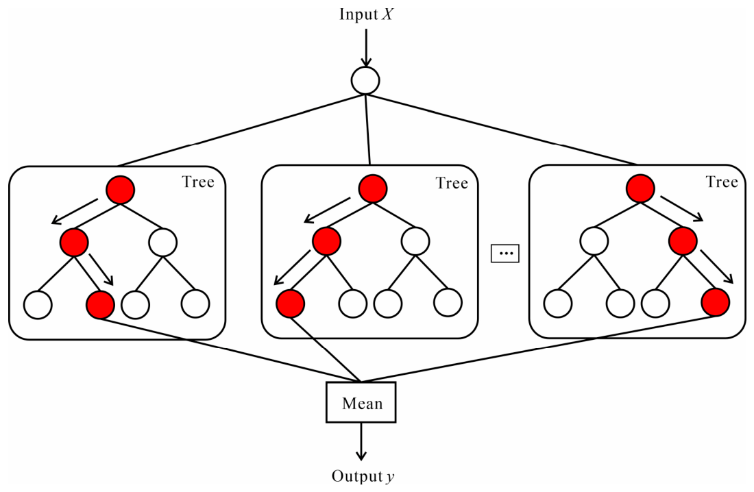
Random forest (RF) combines multiple decision trees for classification and regression tasks [36,37,38,39]. The schematic diagram is shown in Figure 2. The RF algorithm performs a series of random operations after receiving the training data. First, to ensure sample randomness, it randomly draws multiple sub-training sets from the original dataset, ensuring independence among the datasets. Second, the RF algorithm uses these randomly generated training sets to construct independent decision trees. During the construction of each decision tree, feature selection, node generation, and pruning operations are performed to ensure the independence and diversity of each tree. The predictions of individual trees are then aggregated, using voting for classification and averaging for regression.
Figure 2.
Schematic diagram of the RF model. The arrows indicate the direction of data flow through random sampling, decision-tree construction, and prediction aggregation. The red circles highlight randomly selected nodes in the individual decision trees, whereas the white circles represent the remaining nodes.
2.3. Shapley Additive Explanations
Interpretable machine-learning methods have received increasing attention because many predictive models provide limited transparency regarding how individual inputs affect their outputs [30]. In recent years, Lundberg and Lee [40] proposed 22 unified framework, SHAP, to explain predictions. The core idea of SHAP is to measure the effect size of each feature and its interaction term in the model by calculating their Shapley values, which are derived from the Shapley concept in cooperative game theory. SHAP offers the advantage of determining whether each input feature’s contribution is positive or negative and provides a SHAP value for each observation [41].
SHAP includes an explanatory model g, which can be expressed as:
where represents the vector of simplified input variables derived from the original input variables in the dataset; denotes the constant when all input variables are missing; M indicates the number of input features; represents the SHAP value corresponding to the ith feature.
2.4. Indicators for the Assessment
To assess the accuracy of the model, four commonly used evaluation metrics for regression problems were used, as defined in Equations (10)–(13). The mean square error (MSE), root mean square error (RMSE), and mean absolute error (MAE) measure the differences between the predicted and observed values, where lower values indicate better predictive performance. The coefficient of determination (R2) evaluates the predictive agreement between the model outputs and the observed values. An R2 value closer to 1 indicates better predictive performance, whereas R2 can be negative when the prediction error is greater than that obtained using the mean of the observed values as a baseline.
where denotes the true value, denotes the predicted value, denotes the sample average, and m indicates the number of samples.
2.5. Cross-Validation Strategy
To assess the sensitivity of model performance to data partitioning, an additional nested cross-validation analysis was conducted using the 141 macroscopic and microscopic parameter correspondences. Nested cross-validation separates hyperparameter selection from performance evaluation and reduces the optimistic bias that may arise when model tuning and evaluation are performed using the same cross-validation procedure [42]. A similar strategy has recently been applied to machine-learning-assisted DEM parameter calibration [18].
The outer loop employed five-fold cross-validation and was used solely to evaluate the model’s generalization performance. Five-fold and repeated k-fold cross-validation have been adopted in previous geotechnical machine-learning studies to improve the reliability of model evaluation under limited datasets [43,44]. Within each outer training fold, an inner three-fold cross-validation was used for hyperparameter selection.
A compact hyperparameter search space was predefined with reference to commonly used configurations and recent geotechnical machine-learning studies. For DT, the maximum tree depth was set to no limit, 5, or 10, and the minimum number of samples per leaf was set to 1, 3, or 5. For RF, 100 trees were used, while the maximum depth was set to no limit, 5, or 10 and the minimum number of samples per leaf was set to 1 or 5. For XGBoost, the number of estimators was set to 100 or 500, the maximum depth to 2, 3, or 4, and the learning rate to 0.01, 0.05, or 0.10. Hyperparameters were selected according to the mean R2 obtained from the inner folds. The selected model was then evaluated on the corresponding outer test fold, and R2, RMSE, and MAE were summarized as the mean and standard deviation across the five outer folds.
3. Model Training and Result Analysis
3.1. Dataset Preparation
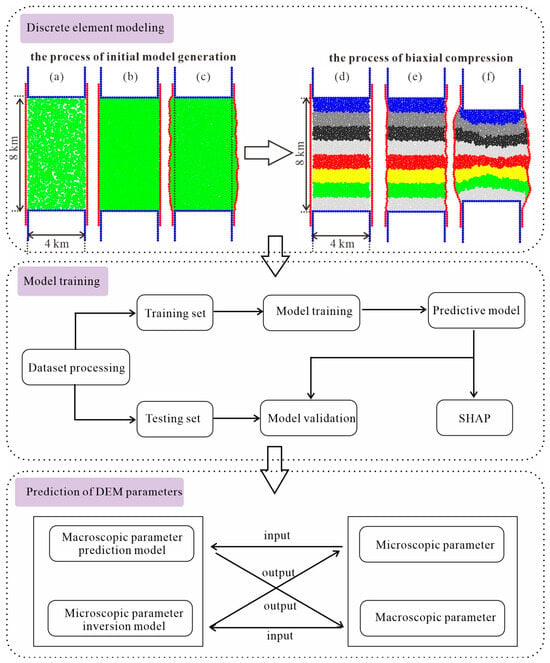
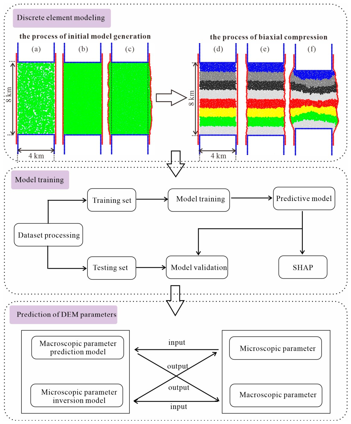
To calibrate the microscopic parameters of the particles and ensure that their macroscopic mechanical responses (e.g., internal friction angle and cohesion) align with indoor test results, this study employs biaxial compression tests and integrates a machine learning approach to establish the mapping relationship between microscopic and macroscopic parameters in the DEM. The flowchart of the DEM macroscopic and microscopic parameters prediction is presented in Figure 3. First, in the DEM modeling part, the high-performance discrete element software ZDEM2D (version 2.2) was used for simulation tests [20,45,46,47,48]. In the field of tectonic geology, 2D discrete element numerical simulation remains a crucial and widely utilized method due to its advantages of faster computation and more intuitive visualization compared to 3D discrete element numerical simulation [49,50,51]. Next, to obtain the corresponding macroscopic parameters of the specimens under different microscopic parameters, biaxial tests were performed and then calculated to obtain the corresponding relationship between the macroscopic and microscopic parameters. However, large-scale rock masses commonly contain fractures and other discontinuities [52]. To represent the overall mechanical response of the rock mass at this scale, a 4 km × 8 km biaxial specimen was constructed [22,47,53,54]. As shown in the discrete element modeling part of Figure 3, the modeling procedure consists of two stages: initial model generation and biaxial compression.
Figure 3.
Flow chart of DEM macroscopic and microscopic parameter prediction. (a) Initial random particle generation; (b) particle radius expansion and system equilibration; (c) lateral relaxation under the prescribed confining pressure; (d) layered specimen before biaxial compression; (e) equilibration following confining pressure application; (f) deformed specimen after biaxial compression. Colors merely aid identification of rock deformation, and particles in one specimen share the same mechanical parameters.
The initial biaxial specimen was generated using the radius expansion method [55,56]. First, four walls composed of particles are generated, and the bond parameters of these particles are set to infinity to prevent fractures [22,47,57]. In a 4 × 8 km area, 2100 particles were randomly generated with the corresponding microscopic parameters, as presented in Table 1 [22,47]. Notably, the friction coefficient of the particles significantly influences their mechanical behavior. Therefore, the friction coefficient was set to 0 during initial model generation. The radius of the particles is then doubled using the radius expansion method to achieve an equilibrium system through calculation. The two side walls were then released, allowing the system to re-equilibrate under the prescribed confining pressure (σ3). Finally, the particle coordinates and radius information within the dashed line are used as the initial model for the biaxial test.
Table 1.
Microscopic parameters of the DEM [22,47].
The biaxial compression process is described as follows: The initial model is transferred to a domain of the same size, where different colors are assigned to distinguish the deformation of different rock layers. In addition, the microscopic and bond parameters of the particles influence the overall mechanical properties of the specimen. The bond parameters were selected to represent the general range of bulk material properties [22,58,59]. Next, the system was equilibrated by calculations with the given contact bond parameters (Table 2) and specified compression velocities for the top and bottom particle walls. Finally, biaxial compression tests were conducted, and the resulting specimen deformation was recorded.
Table 2.
Bond parameters between rock particles [22,47].
Table 1, Table 2 and Table 3 present the microscopic and macroscopic parameters of the DEM, respectively [22,47]. It is noteworthy that we have set the friction coefficient (μ), tensile strength (Tb), and cohesion (Cb) within certain ranges in the microscopic parameters to generate more data on the mapping of macroscopic and microscopic parameters for training machine learning models. Finally, 96 sets of different microscopic parameter combinations were generated, followed by 480 sets (96 × 5) of biaxial compression tests conducted at five different confining pressures (10 MPa, 20 MPa, 40 MPa, 60 MPa, and 80 MPa), resulting in 96 sets of macroscopic and microscopic parameter correspondences. Additionally, along with the 45 sets of macroscopic and microscopic parameter correspondences from Chapter 4 of Li [48], a total of 141 sets of macroscopic and microscopic parameter correspondences were obtained as the training set of the model.
Table 3.
Macroscopic parameters of the DEM [22,47].
3.2. Performance Analysis of Machine Learning Models
After completing the DEM numerical simulation test, the next step is to train the machine learning model. As shown in the model training of Figure 3. This training process typically involves data preprocessing, dataset division, training, model validation, and result analysis. In this study, two prediction models were constructed: a macroscopic parameter prediction model and a microscopic parameter prediction model. To enhance the learning performance of these models, all data were first standardized. The dataset was then randomly split into a training set (80%) and a test set (20%) to facilitate effective model training and validation.
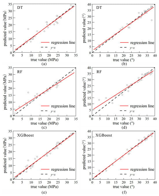
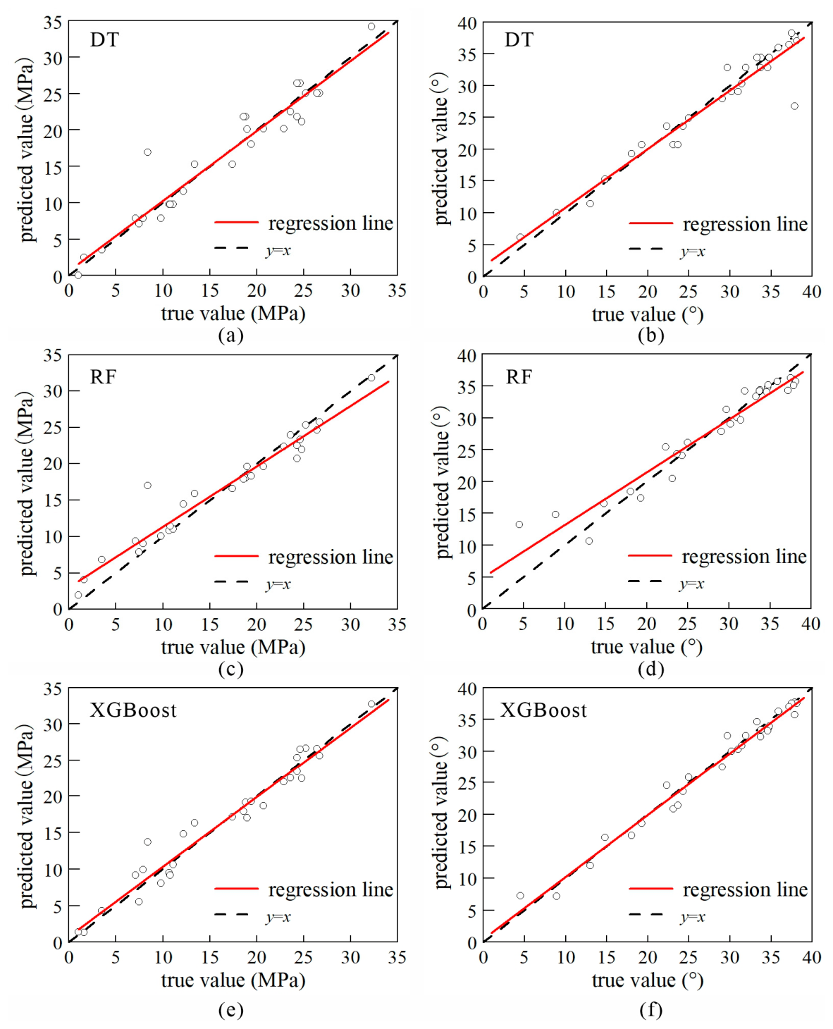
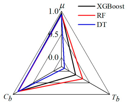
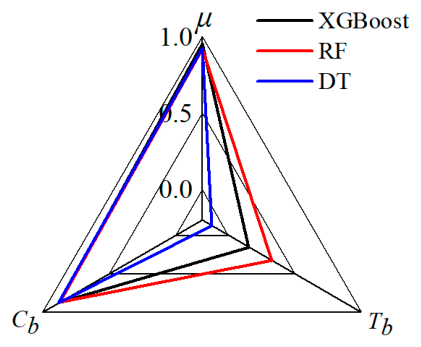
The values of evaluation metrics for various machine learning models in predicting microscopic and macroscopic parameters are presented in Table 4 and Table 5, respectively. Table 4 indicates that the XGBoost model outperforms the DT and RF models in predicting bulk cohesion (Co) and internal friction angle (φ). Figure 4 illustrates the predictions of different models on the test set. Each point in the figures represents a parameter, and its proximity to the y = x line indicates the accuracy of the prediction. Similarly, the regression line represents the overall prediction of the parameters in the test set, and the closer the regression line matches the y = x line, the better the model performs on the test set. Regarding the prediction of microscopic parameters, the XGBoost model excels in predicting the coefficient of friction (μ), while the DT model shows superior performance in predicting cohesion (Cb). In contrast, none of the three models provides satisfactory predictions of tensile strength (Tb), as shown in Figure 5, and the DT model even yields a negative R2 value. According to the definition of R2, this negative value does not necessarily indicate a computational error; rather, it indicates that the predictive performance of the DT model for Tb is poorer than that obtained using the mean of the observed values as a baseline. The consistently lower prediction performance for Tb suggests that the selected macroscopic parameters provide less effective information for constraining this microscopic parameter than for μ and Cb. The limited size and distribution of the current dataset may also contribute to prediction uncertainty. Therefore, the poor prediction of Tb should not be attributed solely to the choice of machine-learning algorithm. Its implications for microscopic-parameter identifiability and inverse calibration are further discussed in Section 5.2.
Table 4.
Results of different machine learning models for predicting macroscopic parameters.
Table 5.
Results of different machine learning models for predicting microscopic parameters.
Figure 4.
Results of the different model for predicting macroscopic parameters. (a,c,e) Co; (b,d,f) φ. The white circles represent the individual samples in the test set.
Figure 5.
Prediction accuracy of the three models.
The nested cross-validation results are summarized in Table 6. For the forward prediction, XGBoost achieved the highest mean R2 for both Co (0.9040) and φ (0.9391), indicating that the strong predictive performance observed in the original train-test evaluation was generally retained across different data partitions. For the inverse prediction, RF and XGBoost showed comparable performance for μ, with mean R2 values of 0.8802 and 0.8795, respectively, while XGBoost achieved the highest mean R2 for Cb (0.8024). In contrast, the prediction of Tb remained substantially less reliable for all three models, with mean R2 values ranging from 0.3190 to 0.4578. The cross-validation results therefore indicate that the overall model performance is not restricted to a single train-test partition, while also confirming the comparatively weak predictability of Tb.
Table 6.
Results of nested five-fold cross-validation for different machine learning models.
3.3. Parameter Sensitivity
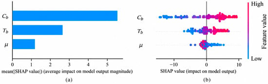
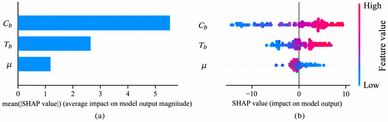
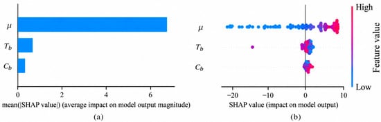
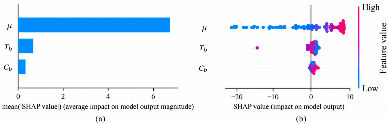
For model selection, the XGBoost model, which has the highest accuracy in predicting macroscopic parameters, was chosen. SHAP was utilized to interpret the prediction results of the XGBoost model. First, the importance of the input features was analyzed to understand their general influence on the predictions. As shown in Figure 6a, the bulk cohesion of rocks is primarily controlled by cohesion and tensile strength, whereas the friction coefficient is less significant for bulk cohesion. Conversely, as depicted in Figure 7a, the friction coefficient strongly influences the internal friction angle, while tensile strength and cohesion have a lesser impact. Figure 6b and Figure 7b present SHAP summary plots that illustrate the effects of the friction coefficient, tensile strength, and cohesion on bulk cohesion and the internal friction angle, respectively. In these plots, each point represents a sample, with red and blue colors indicating the magnitude of the sample values. The horizontal axis represents the SHAP values, and the vertical axis denotes the importance ranking of the features. Figure 6b demonstrates that cohesion and tensile strengths significantly affect bulk cohesion, while Figure 7b shows that the friction coefficient greatly impacts the internal friction angle. These SHAP-derived sensitivity patterns are generally consistent with those obtained from previous DEM control-variable analyses [47]. Their mechanical interpretation and the additional information provided by SHAP relative to conventional sensitivity analysis are further discussed in Section 5.1.
Figure 6.
Interpreting XGBoost model predictions of Co by SHAP values. (a) SHAP feature importance; (b) SHAP summary plot. The grey vertical line in (b) indicates a SHAP value of zero.
Figure 7.
Interpreting XGBoost model predictions of φ by SHAP values. (a) SHAP feature importance; (b) SHAP summary plot. The grey vertical line in (b) indicates a SHAP value of zero.
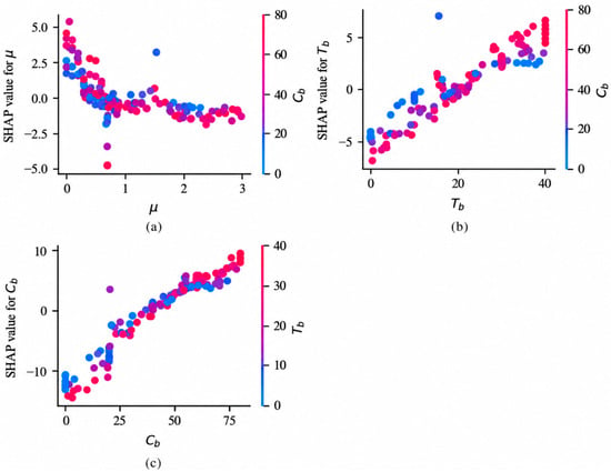
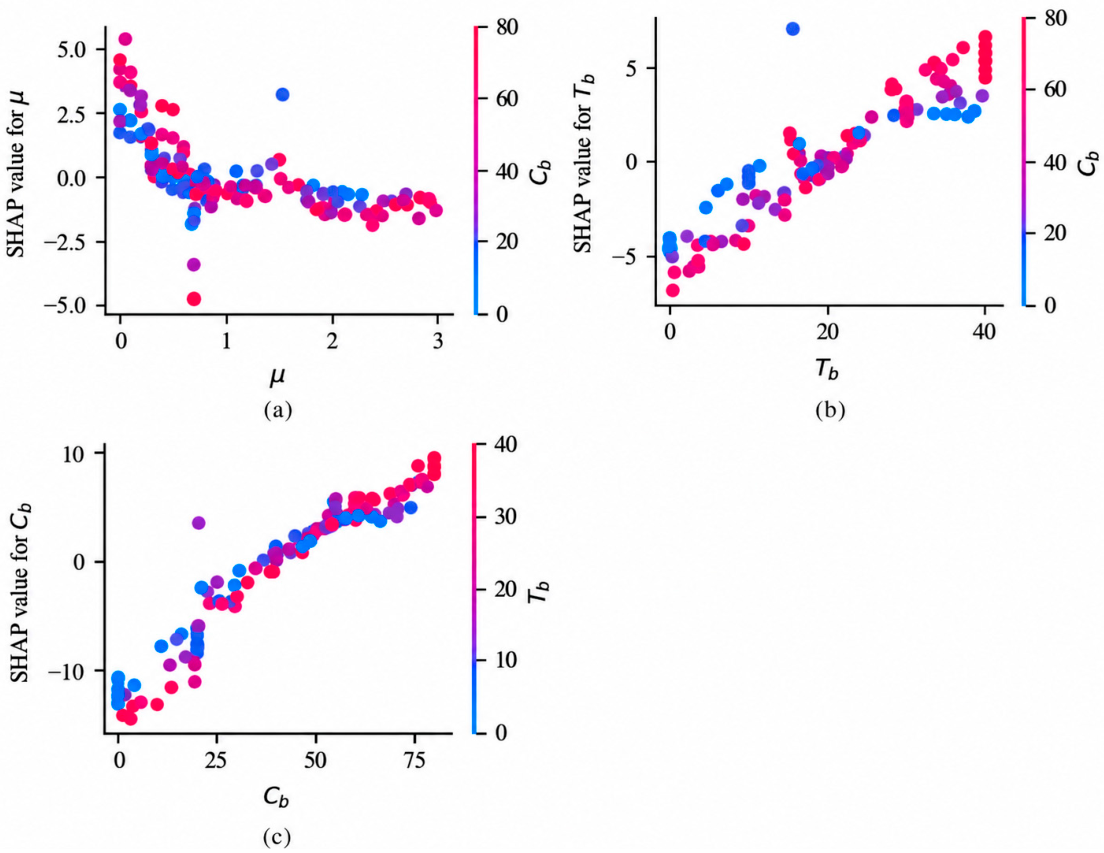
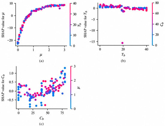
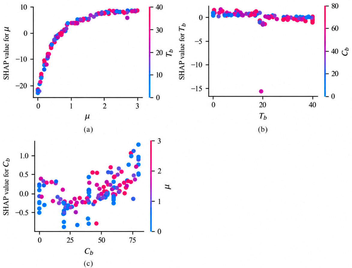
Figure 8 and Figure 9 present the SHAP dependence plots for the microscopic parameters. In each subplot, the horizontal axis represents the value of the corresponding microscopic parameter, whereas the vertical axis represents its SHAP value. The point colors represent the values of Cb, Cb, and Tb, respectively, as indicated by the corresponding color bars. Blue indicates lower parameter values, whereas red indicates higher values.
Figure 8.
SHAP dependence plots for the XGBoost prediction of Co: (a) μ; (b) Tb; (c) Cb.
Figure 9.
SHAP dependence plots for the XGBoost prediction of φ: (a) μ; (b) Tb; (c) Cb.
For the prediction of Co, Figure 8a shows an overall decrease in the SHAP value of μ with increasing μ, whereas the SHAP values of Tb and Cb generally increase with their corresponding parameter values (Figure 8b,c). This indicates that higher Tb and Cb values are generally associated with increasingly positive contributions to the predicted bulk cohesion, whereas the contribution of μ generally decreases as μ increases. For the prediction of φ, Figure 9a shows a pronounced positive and nonlinear relationship between μ and its SHAP contribution, whereas the contributions of Tb and Cb are comparatively smaller (Figure 9b,c).
4. Microscopic Parameter Calibration
Based on the analysis in Section 3, the accuracy of predicting macroscopic parameters using machine learning is satisfactory. It is well known that the choice of microscopic parameters of DEM significantly influences their macroscopic responses. However, directly predicting microscopic parameters from macroscopic parameters using machine learning is less satisfactory. Therefore, a surrogate-assisted calibration framework is adopted by combining the macroscopic-parameter prediction model, SHAP analysis, and differential evolution (DE) to facilitate the calibration of DEM microscopic parameters.
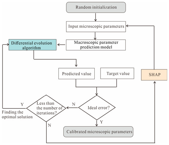
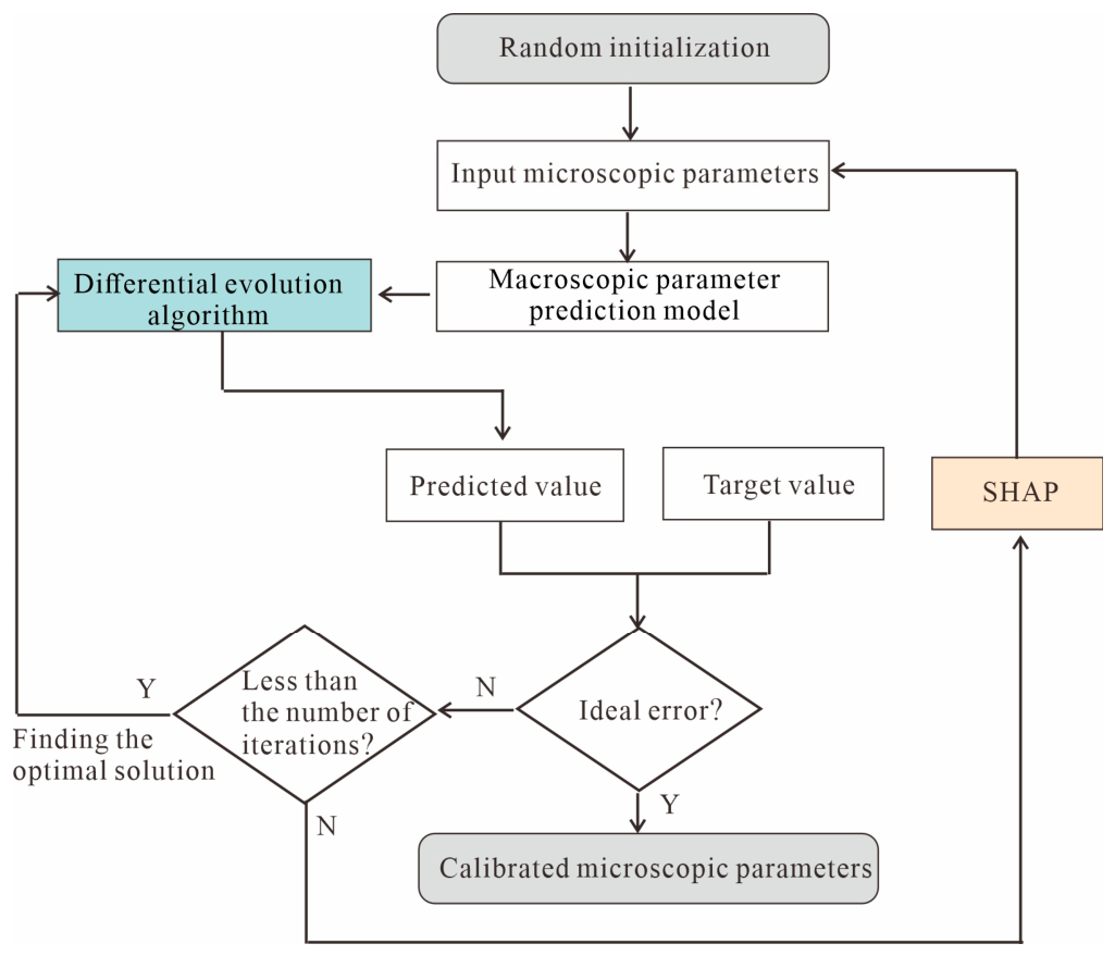
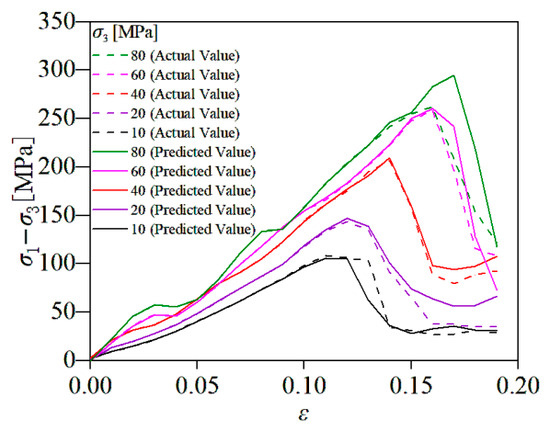
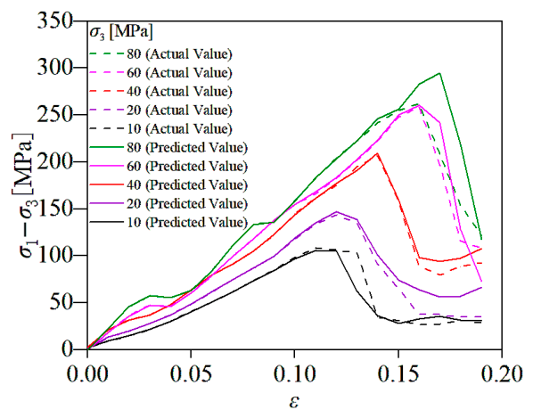
DE is a global optimization algorithm proposed by Storn and Price [60], consisting of initialization, variation, crossover, and selection steps. In this study, the microscopic parameter calibration problem is transformed into a global optimization problem. The microscopic parameter calibration process is illustrated in Figure 10. In the DE algorithm section, experiments are conducted using the “differential_evolution” method from the “SciPy” open-source toolkit (version 1.15.0). Key parameters of “differential_evolution” include the objective function, boundary conditions, target value, and maximum number of iterations. The objective function evaluates the discrepancy between the predicted and target macroscopic parameters. Boundary conditions define the range of input microscopic parameters (Table 1 and Table 2). The target values specify the required macroscopic responses, whereas the maximum number of iterations limits the optimization search. If the iteration limit is reached before the convergence criterion is satisfied, the search terminates without an acceptable solution. At this point, SHAP can be used to analyze the relationship between the macroscopic and microscopic parameters and readjust the input values of the microscopic parameters. Figure 11 demonstrates the stress–strain curves of the real microscopic parameters and the calibrated microscopic parameters, showing the feasibility of the microscopic parameter calibration method proposed in this study.
Figure 10.
Flowchart of microscopic parameter calibration. The arrows indicate the direction of the calibration workflow; Y and N denote “Yes” and “No” branches, respectively, at the decision nodes.
Figure 11.
Stress–strain curves of the real microscopic parameters and the calibrated microscopic parameters.
5. Discussion
5.1. Physical Interpretation and Contribution of SHAP
The SHAP results indicate distinct roles of the microscopic parameters in controlling the predicted macroscopic responses. Bond cohesion Cb and bond tensile strength Tb make the largest contributions to bulk cohesion Co, whereas the friction coefficient μ dominates the prediction of the internal friction angle φ. These trends are mechanically reasonable. Interparticle friction primarily controls resistance to relative sliding and therefore has a direct influence on frictional shear resistance, whereas bond cohesion and tensile strength govern the resistance of bonded contacts to shear and tensile failure. Similar relationships have been identified in conventional DEM sensitivity analyses [48]. More recent bonded-particle calibration studies have also shown that tensile strength, cohesion, and local friction-related parameters contribute differently to macroscopic rock-strength characteristics [61].
The contribution of SHAP in the present study therefore lies not simply in reproducing these previously recognized mechanical relationships. Rather, SHAP provides a quantitative description of the relative importance, direction, and variation in individual parameter contributions over the investigated multidimensional parameter space. Recent DEM calibration studies have similarly introduced SHAP-based interpretation to improve the transparency of surrogate models [17,18]. Zhang et al. combined an XGBoost-based surrogate with SHAP and multi-objective optimization, while Peng et al. employed SHAP together with rigorous model validation to interpret mesoscopic parameter effects [17,18].
Nevertheless, SHAP values describe how the trained surrogate model uses its input features and should not be regarded as independent physical laws. Therefore, the identified contribution patterns should be interpreted together with DEM contact mechanics and conventional numerical sensitivity analyses. In this sense, SHAP complements rather than replaces physics-based interpretation.
5.2. Parameter Identifiability and Model Robustness
The markedly lower prediction performance for bond tensile strength Tb is an important limitation of the direct microscopic-parameter prediction. In contrast to μ and Cb, none of the investigated machine-learning models satisfactorily predicts Tb. This difference suggests that the selected macroscopic responses contain less effective information for constraining Tb. Similar parameter-dependent differences in prediction performance have also been reported in recent machine-learning-based DEM calibration studies [16], indicating that individual microscopic parameters may not be equally recoverable from the same set of macroscopic observations.
This result also raises an identifiability issue in the present inverse problem. Three microscopic parameters, μ, Tb, and Cb, are considered, whereas the calibration targets are bulk cohesion Co and internal friction angle φ. The SHAP results further indicate that φ is predominantly controlled by μ, while Co is jointly influenced by Tb and Cb. Consequently, different combinations of Tb and Cb may potentially produce similar macroscopic responses through parameter compensation. The present results therefore do not guarantee that a unique microscopic parameter set can be identified from the two selected macroscopic targets. The calibrated parameters should instead be interpreted as feasible parameter combinations capable of reproducing the prescribed macroscopic behavior.
Recent rock DEM calibration studies have introduced multiple mechanically distinct responses, such as tensile, uniaxial compressive, and confined compressive strengths, to provide additional constraints on different microscopic parameters [61]. This suggests that incorporating additional observables that are more sensitive to tensile bond failure may improve the constraint on Tb in future calibration.
The robustness of the machine-learning models also requires careful consideration. Although the initial model comparison in Table 4 and Table 5 was based on a single random 80/20 train-test split, an additional nested five-fold cross-validation analysis was conducted to assess the sensitivity of model performance to data partitioning and to provide a more robust estimate of model generalization. As summarized in Table 6, XGBoost retained strong performance for the forward prediction of Co and φ, with mean R2 values of 0.9040 and 0.9391, respectively. For the inverse prediction, μ and Cb also showed comparatively stable performance, whereas Tb remained markedly less predictable across all three models, with mean R2 values ranging from 0.3190 to 0.4578. These results indicate that the principal performance trends are not restricted to a single train-test partition, while also confirming the limited identifiability of Tb under the present macroscopic constraints. Independent forward verification using the original DEM model would provide an additional check on the reliability of the optimized microscopic parameter combinations.
5.3. Practical Implications, Limitations, and Future Work
The practical advantage of the proposed framework lies primarily in reducing repeated DEM calculations during the optimization stage. In the present study, 96 microscopic-parameter combinations were simulated under five confining pressures, resulting in 480 biaxial DEM simulations for database construction. Once the surrogate model is established, candidate microscopic-parameter combinations generated by the DE algorithm can be evaluated directly by the machine-learning model rather than by performing a new DEM simulation for every candidate solution. Therefore, the proposed framework replaces repeated DEM-based trial-and-error evaluations during optimization with surrogate-assisted parameter searching.
It should be emphasized that this advantage does not eliminate the computational cost of constructing the initial DEM database. The benefit of the framework is therefore associated mainly with reducing repeated DEM evaluations during the subsequent calibration stage. Since a direct wall-clock comparison with conventional trial-and-error calibration is not included in the present analysis, the computational advantage is interpreted here in terms of the reduction in repeated DEM evaluations rather than as a quantified speed-up.
Several limitations should also be recognized. First, the surrogate model is based on 141 parameter correspondences and should not be extrapolated beyond the training parameter ranges. Second, only μ, Tb, and Cb are treated as variable microscopic parameters, while Co and φ are used as macroscopic calibration targets. The resulting sensitivity relationships are therefore conditional on the adopted contact model, parameter ranges, model geometry, and loading conditions. Third, the weak identifiability of Tb indicates that additional macroscopic or failure-related observables sensitive to tensile bond failure should be considered. Future work should also use larger and more uniformly distributed datasets, external validation using independent datasets, and independent numerical or experimental verification to further evaluate the robustness and transferability of the proposed framework.
6. Conclusions
In this study, the relationships between macroscopic and microscopic parameters of rock DEM models were investigated using machine-learning methods based on the Hertz–Mindlin bonded contact model. The main conclusions are as follows:
(1) XGBoost provides the best predictive performance for both macroscopic parameters. For microscopic-parameter prediction, μ and Cb exhibit comparatively stronger but model-dependent predictive performance, whereas Tb remains substantially less predictable across all three models. The nested cross-validation results confirm the comparatively weak predictability of Tb, indicating that the selected macroscopic responses provide limited information for uniquely constraining this parameter.
(2) SHAP analysis shows that Cb and Tb make the largest contributions to the prediction of bulk cohesion Co, whereas the contribution of μ is comparatively smaller. Higher Tb and Cb values are generally associated with increasingly positive contributions to the predicted Co. In contrast, μ is the dominant contributor to the prediction of the internal friction angle φ, showing a pronounced positive and nonlinear dependence, while the contributions of Tb and Cb are relatively limited. These results provide a quantitative description of parameter importance and contribution trends within the investigated parameter ranges.
(3) By combining the forward macroscopic prediction model, SHAP, and the DE algorithm, the proposed framework can search for microscopic parameter combinations that reproduce prescribed macroscopic responses. The use of the surrogate model reduces the need to repeatedly perform DEM simulations for every candidate parameter combination during optimization, while SHAP provides interpretable information on parameter contributions that can assist parameter adjustment. The calibrated results should therefore be interpreted as feasible microscopic parameter combinations reproducing the target macroscopic behavior rather than necessarily as unique microscopic solutions.
Author Contributions
Conceptualization, L.L. and C.L.; methodology, C.L. and X.Z.; software, C.L.; validation, L.L.; formal analysis, X.Z.; data curation, X.Z.; writing—original draft preparation, L.L. and X.Z.; writing—review and editing, L.L., C.L., H.D. and D.M.; supervision, H.D., D.M., C.X., Y.D. and Z.C.; project administration, L.L. and C.L.; funding acquisition, L.L. and C.L. All authors have read and agreed to the published version of the manuscript.
Funding
This research was funded by the National Natural Science Foundation of China, grant number 42462025; the 2024 Open Fund Project of the National Engineering Research Center for Oil and Gas Exploration Computer Software, BGP Inc., CNPC, grant number DFWT-ZYRJ-2025-JS-57; the Jiangxi Provincial Natural Science Foundation, grant number 20232BAB213086; the Project of PetroChina Company Limited, grant number 2023D-5008-01; and the China Scholarship Council.
Institutional Review Board Statement
Not applicable.
Informed Consent Statement
Not applicable.
Data Availability Statement
The data that support the findings of this study are available from the corresponding author, upon reasonable request.
Acknowledgments
The authors also appreciate Bingyang Mo from East China University of Technology for providing constructive revision suggestions for this manuscript. The authors would furthermore like to thank the editor and the two anonymous reviewers for their careful evaluation and valuable constructive comments, which have greatly helped improve the quality and clarity of this manuscript.
Conflicts of Interest
Lei Li, Huoxiang Dong, Chen Xu, and Zhaoqin Chen were employed by the company Bureau of Geophysical Prospecting Inc., China National Petroleum Corporation. The authors declare that this study received funding from Bureau of Geophysical Prospecting Inc., China National Petroleum Corporation. The funder was not involved in the study design, collection, analysis, interpretation of data, the writing of this article, or the decision to submit it for publication.
Abbreviations
| Abbreviation | Definition |
| DEM | Discrete Element Method |
| ML | Machine Learning |
| DT | Decision Tree |
| RF | Random Forest |
| XGBoost | Extreme Gradient Boosting |
| SHAP | SHapley Additive exPlanations |
| DE | Differential Evolution |
| CV | Cross-Validation |
| RMSE | Root Mean Square Error |
| MAE | Mean Absolute Error |
| MSE | Mean Square Error |
| R2 | Coefficient of Determination |
References
- Cundall, P.A. A computer model for simulating progressive, large scale movement in blocky rock systems. In Proceedings of the International Symposium on Rock Mechanics; ISRM: Nancy, France, 1971; Volume 2, pp. 129–136. [Google Scholar]
- Cundall, P.A.; Strack, O.D.L. A discrete numerical model for granular assemblies. Geotechnique 1979, 29, 47–65. [Google Scholar] [CrossRef] [Scilit]
- Shentu, J.; Lin, B. A novel machine learning framework for efficient calibration of complex dem model: A case study of a conglomerate sample. Eng. Fract. Mech. 2023, 279, 109044. [Google Scholar] [CrossRef] [Scilit]
- Jiang, J.W.; Ehret, D.; Xiang, W.; Rohn, J.; Huang, L.; Ling, H.; Yan, S.J.; Bi, R. Numerical simulation of Qiaotou Landslide deformation caused by drawdown of the Three Gorges Reservoir, China. Environ. Earth Sci. 2011, 62, 411–419. [Google Scholar] [CrossRef] [Scilit]
- Khazaei, C.; Hazzard, J.; Chalaturnyk, R. Damage quantification of intact rocks using acoustic emission energies recorded during uniaxial compression test and discrete element modeling. Comput. Geotech. 2015, 67, 94–102. [Google Scholar] [CrossRef] [Scilit]
- Luo, S.L.; Ge, H.K.; Wang, J.B.; Zhou, W.; Shen, Y.H.; Liu, P.Y.; Liu, J.T. Numerical simulation study on the crack propagation of conglomerate. R. Soc. Open Sci. 2021, 8, 202178. [Google Scholar] [CrossRef] [Scilit] [PubMed]
- Xue, Y.D.; Zhou, J.; Liu, C.; Shadabfar, M.; Zhang, J. Rock fragmentation induced by a TBM disc-cutter considering the effects of joints: A numerical simulation by DEM. Comput. Geotech. 2021, 136, 104230. [Google Scholar] [CrossRef] [Scilit]
- Yuan, B.; Liu, C.; Qin, Y.; Zhang, T.S.; Ma, X.D. A discrete element modeling of rock and soil material based on the machine learning. IOP Conf. Ser. Earth Environ. Sci. 2021, 861, 032015. [Google Scholar] [CrossRef] [Scilit]
- Zhou, Z.Q.; Bai, S.S.; Chu, K.W.; Li, J.L.; Sun, J.W.; Wang, M.X.; Sun, Y.; Li, M.H.; Liu, Y.H. Calibration of DEM macro and micro parameters via XGBoost method. Granul. Matter 2022, 24, 106. [Google Scholar] [CrossRef] [Scilit]
- Zhou, J.; Liao, X.H.; Chi, Y. Simulating plane strain test of soils by particle flow code. J.-TONGJI Univ. 2002, 30, 1044–1050. [Google Scholar]
- Cheng, K.; Wang, Y.; Yang, Q.; Mo, Y.B.; Guo, Y. Determination of microscopic parameters of quartz sand through triaxial test using the discrete element method. Comput. Geotech. 2017, 92, 22–40. [Google Scholar] [CrossRef] [Scilit]
- Shang, R.; Yang, Y.; Huang, B.; Chen, Y.; Qiu, C.; Liu, W. Calibration and intelligent optimization for DEM numerical parameters in heterogeneous rock mass. Comput. Geotech. 2025, 177, 106863. [Google Scholar] [CrossRef] [Scilit]
- Fan, P.; Chen, J.; Liao, Y.; Zhao, J.; Wang, M. Calibrating the microparameters of DEM models using the ant colony optimization algorithm and the optimal hyperparameters. Sci. Rep. 2025, 15, 16795. [Google Scholar] [CrossRef] [Scilit] [PubMed]
- Zhou, Y.; Wu, S.C.; Jiao, J.J.; Zhang, X.P. Research on mesomechanical parameters of rock and soil mass based on BP neural network. Rock Soil Mech. 2011, 32, 3821–3826. [Google Scholar]
- Benvenuti, L.; Kloss, C.; Pirker, S. Identification of DEM simulation parameters by Artificial Neural Networks and bulk experiments. Powder Technol. 2016, 291, 456–465. [Google Scholar] [CrossRef] [Scilit]
- Jiang, Y.; Pu, J.; Sun, J.; Yao, Z.; Fang, Y.; Ran, Q.; Wang, Y.; Yu, Z. Intelligent calibration method for microscopic parameters in the discrete element method based on ensemble learning. Sci. Rep. 2025, 15, 34923. [Google Scholar] [CrossRef] [Scilit] [PubMed]
- Zhang, Y.; Zhou, X.; Long, G.; Long, Z.; Yang, J. Microparameter calibration method for concrete DEM using metaheuristic-based explainable machine learning and multi-objective optimization. J. Build. Eng. 2025, 112, 113903. [Google Scholar] [CrossRef] [Scilit]
- Peng, C.; Xiang, S.; Liu, W.; Wang, X.; Li, B.; Wu, S. Prediction of compressive strength and calibration of mesoscopic parameters of particle discrete element model based on explainable machine learning. Powder Technol. 2026, 476, 122427. [Google Scholar] [CrossRef] [Scilit]
- Yang, W.M.; Wang, M.X.; Zhou, Z.Q.; Li, L.P.; Yang, G.; Ding, R.S. Research on the relationship between macroscopic and mesoscopic mechanical parameters of limestone based on Hertz Mindlin with bonding model. Geomech. Geophys. Geo-Energy. Geo-Resour. 2020, 6, 68. [Google Scholar] [CrossRef] [Scilit]
- Li, C.S.; Yin, H.W.; Xu, W.Q.; Wu, Z.Y.; Guan, S.W.; Jia, D.; Ren, R. Quantitative Analysis and Simulation of Compressive Tectonics Based on Discrete Element Method. Geotecton. Metallog. 2022, 46, 645–661. [Google Scholar] [CrossRef]
- Johnson, K.L. Contact Mechanics; Cambridge University Press: Cambridge, UK, 1987. [Google Scholar]
- Morgan, J.K. Effects of cohesion on the structural and mechanical evolution of fold and thrust belts and contractional wedges: Discrete element simulations. JGR Solid Earth 2015, 120, 3870–3896. [Google Scholar] [CrossRef] [Scilit]
- Morgan, J.K.; Boettcher, M.S. Numerical simulations of granular shear zones using the distinct element method: 1. Shear zone kinematics and the micromechanics of localization. JGR Solid Earth 1999, 104, 2703–2719. [Google Scholar] [CrossRef] [Scilit]
- Morgan, J.K.; McGovern, P.J. Discrete element simulations of gravitational volcanic deformation: 2. Mechanical analysis. JGR Solid Earth 2005, 110, B05403. [Google Scholar] [CrossRef] [Scilit]
- Chen, T.; Guestrin, C. Xgboost: A scalable tree boosting system. In Proceedings of the 22nd ACM SIGKDD International Conference on Knowledge Discovery and Data Mining, San Francisco, CA, USA, 13–17 August 2016; pp. 785–794. [Google Scholar] [CrossRef] [Scilit]
- Friedman, J.H. Greedy function approximation: A gradient boosting machine. Ann. Stat. 2001, 29, 1189–1232. [Google Scholar] [CrossRef] [Scilit]
- Ramraj, S.; Uzir, N.; Sunil, R.; Shatadeep, B. Experimenting XGBoost algorithm for prediction and classification of different datasets. Int. J. Control Theory Appl. 2016, 9, 651–662. [Google Scholar]
- Shi, X.P.; Wong, Y.D.; Li, M.Z.F.; Palanisamy, C.; Chai, C. A feature learning approach based on XGBoost for driving assessment and risk prediction. Accid. Anal. Prev. 2019, 129, 170–179. [Google Scholar] [CrossRef] [Scilit] [PubMed]
- Zhu, X.; Chu, J.; Wang, K.D.; Wu, S.F.; Yan, W.; Chiam, K. Prediction of rockhead using a hybrid N-XGBoost machine learning framework. J. Rock Mech. Geotech. 2021, 13, 1231–1245. [Google Scholar] [CrossRef] [Scilit]
- Feng, D.C.; Wang, W.J.; Mangalathu, S.; Taciroglu, E. Interpretable XGBoost-SHAP machine-learning model for shear strength prediction of squat RC walls. J. Struct. Eng. 2021, 147, 04021173. [Google Scholar] [CrossRef] [Scilit]
- Klusowski, J.M.; Tian, P.M. Large scale prediction with decision trees. J. Am. Stat. Assoc. 2024, 119, 525–537. [Google Scholar] [CrossRef] [Scilit]
- Mienye, I.D.; Sun, Y.; Wang, Z. Prediction performance of improved decision tree-based algorithms: A review. Procedia Manuf. 2019, 35, 698–703. [Google Scholar] [CrossRef] [Scilit]
- Quinlan, J.R. Induction of decision trees. Mach. Learn. 1986, 1, 81–106. [Google Scholar] [CrossRef] [Scilit]
- Rovnyak, S.; Kretsinger, S.; Thorp, J.; Brown, D. Decision trees for real-time transient stability prediction. IEEE TPS 1994, 9, 1417–1426. [Google Scholar] [CrossRef] [Scilit]
- Song, Y.Y.; Ying, L.U. Decision tree methods: Applications for classification and prediction. Shanghai Arch. Psychiatry 2015, 27, 130. [Google Scholar] [CrossRef] [Scilit] [PubMed]
- Breiman, L. Random forests. Mach. Learn. 2001, 45, 5–32. [Google Scholar] [CrossRef] [Scilit]
- Cutler, D.R.; Edwards, T.C., Jr.; Beard, K.H.; Cutler, A.; Hess, K.T.; Gibson, J.; Lawler, J.J. Random forests for classification in ecology. Ecology 2007, 88, 2783–2792. [Google Scholar] [CrossRef] [Scilit] [PubMed]
- Dong, L.; Li, X.; Peng, K. Prediction of rockburst classification using Random Forest. Trans. Nonferrous Met. Soc. China 2013, 23, 472–477. [Google Scholar] [CrossRef] [Scilit]
- Lariviere, B.; Van den Poel, D. Predicting customer retention and profitability by using random forests and regression forests techniques. Expert Syst. Appl. 2005, 29, 472–484. [Google Scholar] [CrossRef] [Scilit]
- Lundberg, S.M.; Lee, S.I. A unified approach to interpreting model predictions. Adv. Neural Inf. Process. Syst. 2017, 30, 1–10. [Google Scholar] [CrossRef] [Scilit]
- Li, Z.H.; Jiang, S. Reconstructing and Interpreting Analysis of Sonic Logging Curves based on Machine Learning and SHAP Algorithm. Bull. Geol. Sci. Technol. 2024, 44, 321–331. [Google Scholar]
- Varma, S.; Simon, R. Bias in error estimation when using cross-validation for model selection. BMC Bioinform. 2006, 7, 91. [Google Scholar] [CrossRef] [Scilit] [PubMed]
- Gajan, S. Modeling of Seismic Energy Dissipation of Rocking Foundations Using Nonparametric Machine Learning Algorithms. Geotechnics 2021, 1, 534–557. [Google Scholar] [CrossRef] [Scilit]
- Zeini, H.A.; Seno, M.E.; Shehab, E.Q.; Abood, E.A.; Imran, H.; Bernardo, L.F.A.; Ribeiro, T.P. Predicting the Bearing Capacity of Shallow Foundations on Granular Soil Using Ensemble Machine Learning Models. Geotechnics 2025, 5, 57. [Google Scholar] [CrossRef] [Scilit]
- Li, C.S.; Yin, H.W.; Liu, C.; Cai, S.Y. Design and Test of Parallel Discrete Element Method Program of Shared Memory Type. J. Nanjing Univ. (Nat. Sci.) 2017, 53, 1161–1170. [Google Scholar]
- Li, C.S.; Yin, H.W.; Jia, D.; Zhang, J.X.; Wang, W.; Xu, S.J. Validation tests for discrete element codes using single-contact systems. Int. J. Geomech. 2018, 18, 06018011. [Google Scholar] [CrossRef] [Scilit]
- Li, C.S. Quantitative Analysis and Simulation of Structural Deformation in the Fold and Thrust Belt Based on Discrete Element Method. Ph.D. Thesis, NanJing University, Nanjing, China, 2019. (In Chinese with English abstract). [Google Scholar]
- Li, C.S.; Yin, H.W.; Wu, C.; Zhang, Y.C.; Zhang, J.X.; Wu, Z.Y.; Wang, W.; Jia, D.; Guan, S.W.; Ren, R. Calibration of the discrete element method and modeling of shortening experiments. Front. Earth Sci. 2021, 9, 636512. [Google Scholar] [CrossRef] [Scilit]
- Hardy, S. Discrete element modelling of extensional, growth, fault-propagation folds. Basin Res. 2019, 31, 584–599. [Google Scholar] [CrossRef] [Scilit]
- Mao, Z.; Zeng, L.B.; Liu, G.D.; Liu, G.P.; Tian, H.; Dong, S.Q.; Lyu, Y.; Ostadhassan, M. Controls of fault-bend fold on natural fractures: Insight from discrete element simulation and outcrops in the southern margin of the Junggar Basin, Western China. Mar. Pet. Geol. 2022, 138, 105541. [Google Scholar] [CrossRef] [Scilit]
- Zhou, C.; He, J.K.; Su, H.; Wang, W.M.; Wang, X.G.; Zhao, Y.J.; Jiang, Y. Discrete element modeling of distal deformation propagation in thrust wedge and implications for early deformation on northern Tibetan and Iranian Plateaus. J. Struct. Geol. 2024, 184, 105150. [Google Scholar] [CrossRef] [Scilit]
- Germanovich, L.N.; Salganik, R.L.; Dyskin, A.V.; Lee, K.K. Mechanisms of brittle fracture of rock with pre-existing cracks in compression. Pure Appl. Geophys. 1994, 143, 117–149. [Google Scholar] [CrossRef] [Scilit]
- Botter, C.; Cardozo, N.; Hardy, S.; Lecomte, I.; Escalona, A. From mechanical modeling to seismic imaging of faults: A synthetic workflow to study the impact of faults on seismic. Mar. Pet. Geol. 2014, 57, 187–207. [Google Scholar] [CrossRef] [Scilit]
- Maxwell, S.A. Deformation Styles of Allochthonous Salt Sheets During Differential Loading Conditions: Insights from Discrete Element Models. Master’s Thesis, Rice University, Houston, TX, USA, 2009. [Google Scholar]
- Itasca Consulting Group. PFC2D Users’ Manual (Version 3.1); Itasca Consulting Group Inc.: Minneapolis, MN, USA, 2004. [Google Scholar]
- Wang, Y.N.; Tonon, F. Modeling Lac du Bonnet granite using a discrete element model. Int. J. Rock Mech. Min. 2009, 46, 1124–1135. [Google Scholar] [CrossRef] [Scilit]
- Zhang, J.Q.; Wang, X.; Yin, Z.Y.; Liang, Z.Y. DEM modeling of large-scale triaxial test of rock clasts considering realistic particle shapes and flexible membrane boundary. Eng. Geol. 2020, 279, 105871. [Google Scholar] [CrossRef] [Scilit]
- Camac, B.A.; Hunt, S.P.; Boult, P.J. Predicting brittle cap-seal failure of petroleum traps: An application of 2D and 3D distinct element method. Petrol. Geosci. 2009, 15, 75–89. [Google Scholar] [CrossRef] [Scilit]
- Schumann, K.; Behrmann, J.H.; Stipp, M.; Yamamoto, Y.; Kitamura, Y.; Lempp, C. Geotechnical behavior of mudstones from the Shimanto and Boso accretionary complexes, and implications for the Nankai accretionary prism. Earth Planets Space 2014, 66, 129. [Google Scholar] [CrossRef] [Scilit]
- Storn, R.; Price, K. Differential evolution–a simple and efficient heuristic for global optimization over continuous spaces. J. Glob. Optim. 1997, 11, 341–359. [Google Scholar] [CrossRef] [Scilit]
- Zhou, X.; Xu, H.; Gong, Q.; Ma, Y.; Xie, W. An analytical optimal calibration framework of bonded particle model for rock strength envelop modelling. Sci. Rep. 2025, 15, 17162. [Google Scholar] [CrossRef] [Scilit] [PubMed]

Disclaimer/Publisher’s Note: The statements, opinions and data contained in all publications are solely those of the individual author(s) and contributor(s) and not of MDPI and/or the editor(s). MDPI and/or the editor(s) disclaim responsibility for any injury to people or property resulting from any ideas, methods, instructions or products referred to in the content. |
© 2026 by the authors. Licensee MDPI, Basel, Switzerland. This article is an open access article distributed under the terms and conditions of the Creative Commons Attribution (CC BY) license.