


Abstract
Japan’s Location Optimization Plans designate Residential and Urban Function Guidance Zones, but their outcomes for non-commuting, non-school access to daily services are rarely screened against the spatial reorganization they require. This study pairs the Urban Spatial Reorganization Distance (USRD), an exact optimal-transport, latent-demand-weighted measure of minimum reorganization, with the Urban Mobility Efficiency Index (UMEI), a demand-based measure of mobility energy normalized by the 2020 Census municipal population. Across 305 municipalities, median exact USRD was 2.45 km; 205 (67.2%) improved under full realization with a fixed transit network, whereas 100 (32.8%) did not. Total USRD was not monotonically associated with UMEI improvement (Spearman , ), but non-improvement was concentrated in designated and core cities and accompanied by lengthened modeled trips. Compactness can therefore worsen service-access efficiency when residential and destination zones are spatially misaligned. The USRD–UMEI matrix is a screening framework, not an estimate of financial implementation cost.
1. Introduction
1.1. Background: Urban Policy Challenges in an Era of Population Decline
Japan faces the dual challenge of rapid population decline and aging urban service systems. The national population, which peaked at approximately 128 million in 2008, is projected to fall below 100 million by 2050 [1]. This demographic shift has intensified concerns about the sustainability of dispersed urban structures. In many Japanese cities where automobile-dependent suburban sprawl has progressed, municipalities must continue to provide public facilities, daily services, and transportation across wide urbanized areas with thinning populations.
As a policy response to these challenges, the Japanese government introduced the Location Optimization Plan (LOP; Ritchi Tekiseika Keikaku) system through the 2014 revision of the Act on Special Measures for Urban Revitalization. The system aims to guide population and urban services toward compact, transit-accessible cores through the designation of Residential Guidance Zones (Kyojū Yūdō Kuiki) and Urban Function Guidance Zones (Toshi Kinō Yūdō Kuiki). As of 2025, over 600 municipalities have formulated or are formulating LOPs, making this one of the world’s largest-scale experiments in planned urban compaction.
At its core, the LOP system designates two kinds of guidance zones: Residential Guidance Zones, which serve as origins, and Urban Function Guidance Zones, which contain destinations for daily services. Formulating a compact city plan is thus a long-term decision about where to locate the two ends of service-access trips. The present analysis is deliberately limited to non-commuting and non-school activities represented by the latent travel demand data; it does not measure the full daily trip portfolio. Within that scope, a plan may appear coherent as a long-term spatial design while still lengthening trips if origins and destinations are guided to poorly matched locations; conversely, even a modest realignment can reduce the mobility-energy burden. Evaluating a compact city plan therefore requires two complementary indicators: one capturing the scale of the intended spatial rearrangement and one capturing its consequence for service-access mobility energy.
The non-commuting, non-school service-access mobility dimension is especially consequential because the sustainability of public transportation has become a pressing challenge in depopulating regions. Declining ridership has led to service reductions and route cancellations, creating a vicious cycle in which reduced service further accelerates automobile dependence and population outflow from transit-served areas. Numerous empirical studies since Newman and Kenworthy [2] have confirmed a strong negative relationship between urban density and transport energy consumption—a relationship also documented for Japanese cities through time-series analyses of automobile CO2 emissions and urban structure [3]—suggesting that compact spatial structures can support viable public transportation by concentrating demand along transit corridors. The LOP system represents an institutional attempt to coordinate residential locations, urban functions, and public transportation through planned spatial consolidation. Compact urban form has also been discussed in relation to infrastructure maintenance burden and public service efficiency [4,5]; the present study, however, focuses on the spatial arrangement of guidance zones and its consequences for service-access mobility, which lie at the heart of the LOP system.
1.2. International Context: The Global Spread of Compact City Policies and the Evaluation Challenge
While the LOP system is one of the world’s largest experiments in planned urban compaction, the broader policy of consolidating population and functions to curb automobile dependence has been pursued widely across countries. Compact urban development in the Dutch Randstad [6], Europe’s Sustainable Urban Mobility Plans (SUMPs), and the more recent proximity planning agenda epitomized by the “15-Minute City” [7] all share the LOP’s core concern: reducing the mobility burden by reorganizing the spatial relationship between residences and the destinations of daily life. The recognition that the spatial proximity between origins (residences) and destinations (workplaces and urban functions) governs travel distance and energy consumption has a long lineage in the jobs–housing balance literature [8,9], and destination accessibility has repeatedly been found to be among the strongest predictors of vehicle miles traveled [10]. The residential–functional balance that this study addresses thus sits within an established tradition of international urban and transport planning research.
At the same time, the problem that compaction does not necessarily deliver the expected mobility improvements has been repeatedly documented abroad. An ex post evaluation of thirty years of Dutch compact city policy concluded that the effects of the policy were not well understood and that its achievements in the mobility dimension in particular were limited [11]. A recent analysis of shrinking Korean cities concludes that compaction pursued through uniform increases in residential density may not improve commuting efficiency, and that selective consolidation of employment functions aligned with public transit and residential areas—that is, securing jobs–housing balance—is what proves effective [12]. This mirrors the present study’s finding that compaction can worsen mobility efficiency when Residential and Urban Function Guidance Zones are spatially misaligned. Skepticism about the cost-effectiveness of the compact city itself also has a long history [13].
More importantly, the absence of a quantitative basis for comparing the spatial burden and mobility gain of reorganization ex ante is not unique to Japan but is an internationally shared challenge. The OECD, in its comparative assessment of member countries’ compact city policies, emphasized the need for internationally comparable indicators and proposed 18 core indicators [4]; these, however—such as trip distance and the matching of services with homes—are ex post monitoring indicators rather than design criteria for comparing a proposed guidance-zone configuration before it is finalized. Europe’s SUMPs likewise lack a standardized burden–gain metric, and even the 15-Minute City concept still lacks standardized methods for measuring proximity [7,14]. In “smart shrinkage” plans in the United States (e.g., Youngstown, Ohio), plans have been formulated but the mechanisms for implementation and evaluation remain weak, resulting in large gaps between planning intent and actual land-use change [15]. The two problems addressed below—that plans lack an ex ante evaluation basis and that existing indicators do not jointly represent spatial reorganization and mobility outcomes—are therefore common to countries pursuing planned compaction, not to the Japanese LOP alone.
1.3. The Evaluation Gap
However, the LOP system lacks a mechanism for verifying ex ante whether the guidance-zone configurations set by individual plans are spatially coherent and mobility-efficient. While the system defines procedures for zone designation through guidelines, it provides no quantitative criteria for comparing the reorganization burden and mobility gain of alternative configurations.
Related descriptive work has examined how LOPs and Regional Public Transport Plans document their objectives, zone-setting methods, and effect-measurement procedures [16]. The present study does not reanalyze or make empirical claims from those document codes. It addresses the narrower methodological problem of providing a reproducible quantitative screen for guidance-zone configurations.
1.4. Limitations of Existing Evaluation Indicators
An external framework for comparing reorganization burden and mobility outcomes is therefore useful. Existing approaches do not adequately meet this need.
No spatial-burden indicator has been established for this purpose. Existing measures of plan implementation progress (e.g., population share within guidance zones) assess the state after plan realization, not how far a proposed zone configuration diverges from the current demand-weighted spatial patterns of trip origins and destinations.
Mobility-outcome indicators also have limitations. Supply-side coverage metrics—such as the share of population within walking distance of public transit stops—measure the availability of opportunities but do not capture the energy required to satisfy travel demand. Ever since accessibility was formalized as a determinant of land use [17], the accessibility literature has noted that supply-side measures inadequately reflect residents’ demand satisfaction and behavior [18,19]. More detailed mobility indicators often require household travel surveys and are difficult to apply nationally. The closest prior effort—a cost-and-effect simulation model for compact city approaches in Japan [20]—demonstrates the value of considering implementation costs and mobility effects jointly, but is a single-city case study. Unlike a comprehensive economic cost–benefit analysis, which can monetize multiple benefits and externalities [21], the present framework deliberately compares a geometric reorganization distance with a physical mobility-energy change and must not be interpreted as a fiscal appraisal.
1.5. Approach and Contributions of This Study
This study develops a quantitative screening framework based on the Urban Spatial Reorganization Distance (USRD) and the Urban Mobility Efficiency Index (UMEI). USRD is the sum of two exact 1-Wasserstein distances: one from the current LTD trip-origin demand distribution to the distribution supported within Residential Guidance Zones, and one from the current LTD trip-destination demand distribution to the distribution supported within Urban Function Guidance Zones. UMEI is a demand-based indicator of the mobility-energy burden (MJ/person/day) for the non-commuting, non-school service-access activities represented in the LTD data, normalized by the 2020 Census municipal population. Their integration provides a nationally comparable burden–gain assessment without claiming to measure financial implementation cost.
1.6. Research Questions and Paper Organization
This study addresses two research questions:
- RQ1: What is the relationship between USRD (spatial reorganization burden) and UMEI (plan effect) across Japanese municipalities?
- RQ2: What urban structural and plan-design differences distinguish municipalities with favorable and unfavorable reorganization-burden–mobility-gain profiles?
The remainder of this paper is organized as follows. Section 2 presents the theoretical framework. Section 3 details the evaluation framework design. Section 4 describes the data and analytical methods. Section 5 presents the results of the USRD and UMEI computations. Section 6 discusses the findings and policy implications. Section 7 concludes.
2. Theoretical Framework
2.1. Two Questions for Plan Evaluation
Evaluating a compact city plan requires answering two fundamentally distinct questions:
- How spatially divergent is the plan? What minimum geometric reorganization separates the current LTD trip-origin and trip-destination demand distributions from the distributions supported within the corresponding guidance zones? This is a question about the spatial reorganization burden a plan implies under LTD demand weighting, not its practical feasibility.
- Would the plan be effective within the modeled scope? If the planned spatial reorganization were achieved, would non-commuting, non-school service access become more energy-efficient? This is a question about modeled mobility gain.
These two dimensions are conceptually independent. A plan may require minimal reorganization (a low burden) because its guidance zones closely match the current trip-origin and trip-destination demand distributions, yet yield little efficiency improvement precisely because it changes so little. Conversely, an ambitious plan requiring substantial reorganization (a high burden) might—or might not—produce large efficiency gains, depending on whether the target zones are well-served by public transit.
Table 1 summarizes this two-dimensional structure.
Table 1.
Two-dimensional structure of plan evaluation.
Existing evaluation approaches typically address only one of these dimensions: coverage metrics assess whether zones are well located, while accessibility measures assess potential benefits. The proposed framework integrates both dimensions through USRD and UMEI.
2.2. The Urban Spatial Reorganization Distance as a Measure of Spatial Reorganization Burden
We measure the spatial reorganization burden that a plan implies with the Urban Spatial Reorganization Distance (USRD), an indicator introduced in this study and computed from the LTD trip-origin and trip-destination demand distributions. USRD is a geometric, demand-weighted measure of how far the current origin–destination demand structure is from the structure supported within a plan’s guidance zones; it is not an estimate of the monetary cost of implementing the plan. The underlying metric—the 1-Wasserstein distance, also known as the Earth Mover’s Distance (EMD) or the Kantorovich–Rubinstein metric—originates from the optimal-transport problem formalized by Monge [22] and generalized by Kantorovich [23], and has since found applications across economics, traffic, and urban planning [24]. What is specific to this study is not the metric but the construct built on it: separate target distributions are derived from Residential and Urban Function Guidance Zones, each LTD demand component is normalized to its total municipal source mass, and the result is decomposed into origin-side and destination-side distances. For two probability distributions and over a metric space , the 1-Wasserstein distance is defined as
where is the set of all joint distributions (transport plans) with marginals and [25].
In the context of compact city evaluation, we interpret this as follows:
- Source distribution (): the current spatial distribution of LTD trip-origin demand for , or LTD trip-destination demand for , across 500 m grid cells within a municipality;
- Target distribution (): the same total origin or destination demand supported only at cells inside the corresponding guidance zones and allocated in proportion to the current within-zone source mass;
- Ground metric (d): great-circle distance between grid-cell centroids (km), computed with the haversine formula;
- USRD value: the minimum mass-weighted mean displacement distance (km) required to transform the current distribution into the planned one. Because and are normalized to probability distributions, USRD is expressed in kilometers and represents the demand-weighted mean distance over which mass must be displaced; it is not a total person-kilometer count, and it is a geometric measure of the magnitude of reorganization rather than a monetary cost.
Critically, USRD provides an optimistic lower-bound measure of the spatial displacement of the modeled LTD demand mass required for plan realization, not a lower bound on monetary implementation cost—the two have different units and are not directly comparable. Real-world changes in residential locations and service provision involve land acquisition, infrastructure development, incentive programs, facility decisions, and decades of gradual adjustment—all of which incur costs that are not represented by the geometric minimum. USRD thus measures not actual implementation cost, but the structural ambition of the plan under LTD demand weighting: how far the zone-supported origin and destination distributions diverge from their current spatial patterns.
We compute two components: for the LTD trip-origin demand associated with Residential Guidance Zones and for the LTD trip-destination demand associated with Urban Function Guidance Zones, with the total reorganization distance defined as .
2.3. UMEI as a Measure of Plan Benefit
The Urban Mobility Efficiency Index (UMEI) quantifies the daily mobility-energy burden imposed by urban spatial structure on residents. It is defined as the total energy consumption (in MJ) required to satisfy the daily travel demand represented in the LTD dataset—that is, the non-commuting, non-school activity demand derived from time use activity rates (Section 3.3)—divided by the municipality’s resident population in the 2020 Population Census:
where
- : travel demand between origin o and destination d (persons/day);
- : travel distance between o and d (km), obtained as times the great-circle distance between the mesh centroids, where is a detour coefficient applied uniformly to both transit and automobile travel to approximate network distance;
- : probability of public transit use for the O-D pair;
- : energy intensity of public transit for the O-D pair (MJ/person-km). If either endpoint’s selected access node is rail, the rail value 0.3 is used; the bus value 0.9 is used only when both selected nodes are bus stops. This is a deterministic access-node rule, not a blended rail–bus rate;
- : energy intensity of automobile travel (2.0 MJ/person-km);
- : resident population of municipality m in the 2020 Population Census (persons).
The LTD total is a generated daily activity-demand count and can exceed the resident population because one resident may generate more than one modeled activity. It is therefore not used as UMEI’s population denominator. The same Census population is used for current and future conditions, for each day type, and in all sensitivity scenarios. This makes the numerator’s daily mobility energy (MJ/day) and the reported unit (MJ/person/day) dimensionally consistent.
UMEI differs from conventional accessibility measures in three key respects:
- Demand-based: Rather than measuring what opportunities are available (supply-side), UMEI quantifies the energy required to satisfy all service-access travel demand represented in the LTD dataset, including latent demand from mobility-disadvantaged populations. The tendency for travel needs to be suppressed among elderly and non-car-owning populations when transit is inadequate has been emphasized in the transport social exclusion literature [26,27]; by adopting the design philosophy that demand must be met, UMEI does not undercount the costs of poor spatial structure.
- Energy as a common unit: By converting all travel into energy (MJ/person/day), UMEI enables direct comparison across municipalities with different sizes, transit systems, and spatial structures. Unlike dimensionless accessibility indices, the energy unit has physical meaning and policy relevance.
- Mode-choice integration: The transit use probability is not a behavioral parameter estimated from surveys but a structural accessibility measure computed from the spatial and temporal characteristics of the transit network. This allows UMEI to be computed from universally available data (transit schedules, population grids, O-D matrices) without requiring household travel surveys.
2.4. The Two-Dimensional Framework: USRD × UMEI
The plan’s improvement effect is measured as the change in UMEI between the current state and the plan realization scenario:
where positive values indicate improvement (lower energy consumption under the plan). USRD and UMEI retain different physical units and are therefore evaluated as two separate axes rather than collapsed into a ratio. Whether a configuration is financially, legally, politically, or socially feasible requires separate evidence.
2.5. The Residential–Functional Balance: Why Two Components Matter
A critical insight of the two-component USRD structure () is that effective compact city plan design requires balancing the configurations of Residential and Urban Function Guidance Zones. This balance is essential because UMEI depends not on the independent concentration of either population or urban functions, but on the spatial relationship between where people live and where they access services. This logic applies the jobs–housing balance literature—which holds that spatial alignment between residences and destinations (workplaces) shortens travel distances [8,9,10]—to the LOP-specific structure of Residential and Urban Function Guidance Zones.
Three imbalance scenarios illustrate this point:
- Function-only concentration: If urban functions are concentrated into guidance zones without corresponding residential concentration, residents outside the zones must travel longer distances to access consolidated services. This can worsen mobility efficiency despite achieving functional consolidation—a pattern that may explain the negative UMEI observed in some larger municipalities.
- No concentration: If neither population nor functions are concentrated, no compactness benefit is realized. The plan merely endorses the status quo, yielding low USRD but also low UMEI.
- Over-concentration of both: If both population and functions are aggressively concentrated into narrow zones, becomes very high, potentially undermining feasibility. Moreover, unless the concentrated zones align well with existing transit corridors, the resulting spatial structure may not improve mobility efficiency proportionally.
The UMEI framework captures this balance directly: UMEI improves only when the spatial reorganization brings residential locations and service destinations into a configuration that is more transit-efficient, not merely when either dimension is independently consolidated. This sensitivity to the residential–functional balance is a central feature of the proposed framework and distinguishes it from single-dimension compactness metrics that assess population concentration or service accessibility in isolation.
3. Evaluation Framework Design
3.1. Overall Framework Structure
The evaluation framework proceeds in five steps:
- Latent travel demand estimation: Estimate O-D travel demand at 500 m mesh resolution using population distribution, activity rates, and facility distribution (Section 3.3);
- Current UMEI computation: Calculate UMEI for the current spatial distribution of population and urban functions using the estimated demand matrices (Section 3.4);
- USRD computation: Measure the minimum displacement distance from the current LTD trip-origin and trip-destination demand distributions to their zone-supported target distributions (Section 3.2);
- Future UMEI computation: Calculate UMEI under the plan realization scenario, where LTD trip-origin and trip-destination demand are redistributed into their corresponding guidance zones (Section 3.5);
- UMEI and two-dimensional classification: Compute the improvement in mobility efficiency, position each municipality on the USRD ×UMEI matrix, and classify it into one of four quadrants (Section 3.6).
3.2. USRD Computation
3.2.1. Source and Target Distributions
For residential-origin USRD ():
- Source: Current LTD trip-origin demand at 500 m mesh level, generated from the population grid and time use activity rates;
- Target: The same total trip-origin demand supported within Residential Guidance Zones and allocated proportionally to existing within-zone trip-origin demand.
For urban-function-destination USRD ():
- Source: Current LTD trip-destination demand at 500 m mesh level;
- Target: The same total trip-destination demand supported within Urban Function Guidance Zones and allocated proportionally to existing within-zone trip-destination demand.
3.2.2. Exact Optimal Transport
USRD is computed as the unregularized 1-Wasserstein distance in Equation (1), using the network-simplex implementation in POT (Python Optimal Transport) v0.9.6 (ot.emd). No entropic penalty enters the main estimate. The ground-cost matrix contains pairwise great-circle distances between mesh centroids, calculated with the haversine formula.
The target support is a subset of the source support and, at every within-zone point, target mass is at least its current source mass because total municipal mass is reallocated in proportion to existing within-zone mass. Under a metric ground cost, an optimal plan can therefore retain all existing within-zone mass at its original point at zero distance: if within-zone mass were sent elsewhere while another point supplied its original location, the two flows could be exchanged without increasing cost by the triangle inequality. We fix these self-flows and solve the reduced exact problem from out-of-zone source mass to the remaining proportional capacity at within-zone targets. USRD is the resulting total transport cost divided by total municipal mass, so unmoved within-zone mass remains in the denominator. Full and reduced formulations were compared on validation cases, and source and target marginal errors were required to remain below in normalized mass.
Archived entropically regularized Sinkhorn estimates at and km are reported only as a supplementary approximation-sensitivity audit (Supplementary Figure S1 and its accompanying municipality-level data) [28,29]; they are not treated as convergence-certified estimates of the unregularized distance.
3.2.3. Output
Each municipality receives the following USRD values:
- : residential-origin-demand reorganization distance (km)
- : urban-function-destination-demand reorganization distance (km)
USRD and UMEI are computed separately for Saturday, Sunday, and weekday demand because the demand-weighted source distributions vary by day type even though the guidance-zone geometry is fixed. The municipality-level results reported below are the unweighted means of these three day-type estimates.
3.3. Latent Travel Demand Estimation
UMEI requires spatially explicit O-D travel demand as input. Conventional travel demand data—person trip surveys, four-step estimation models, and activity-based models—are either unavailable for most small and medium-sized municipalities, capture only manifest (realized) travel, or require prohibitive data acquisition and computational resources. To overcome these limitations, this study adopts the latent travel demand (LTD) estimation method proposed by Kobayashi [30], which estimates demand from three openly available datasets at 500 m mesh resolution without requiring household travel surveys.
3.3.1. Conceptual Foundation
The LTD method is grounded in the activity-based understanding of travel demand [31,32]. Following the framework of Clifton and Moura [33], which conceptualizes latent travel demand as progressing through stages from desire to intention, planning, scheduling, and realization, LTD is defined as the number of desired activities requiring travel at the planning and scheduling stage—that is, demand that exists regardless of whether adequate transportation is available. This distinction is critical for compact city evaluation: in areas with insufficient public transportation, manifest travel volumes underrepresent actual mobility needs, whereas LTD captures the demand that urban spatial structure must accommodate.
3.3.2. Estimation Procedure
The LTD estimation combines three data sources (Figure 1):
Figure 1.
Conceptual diagram of the latent travel demand (LTD) estimation. Three open-data sources (population distribution, activity rates, and facility distribution) are combined in two steps to generate an origin–destination latent demand matrix, which serves as the common input to the UMEI and USRD computations.
- Population distribution (who, from where): The 500 m mesh population grid obtained from the MLIT National Land Numerical Information database and derived from the 2020 National Census, disaggregated by age and sex, provides the spatial distribution of potential trip origins.
- Activity rates (when, who, for what purpose): Time use data from the NHK Time Use Survey (NHK Broadcasting Culture Research Institute), which provides the proportion of the population engaged in specific activities by age, sex, time of day, and day type (weekday/weekend). Activities requiring travel are identified and categorized by purpose (e.g., medical treatment, shopping, dining, leisure, childcare, sports, household errands).
- Facility distribution (for what purpose, to where): The locations of destination facilities (hospitals, supermarkets, restaurants, parks, childcare centers, etc.) obtained from publicly available map data, which define potential trip destinations by activity type.
The estimation proceeds in two steps:
Step 1—Travel activity population: For each 500 m mesh cell, time period, and activity type, the resident population is multiplied by the corresponding activity rate and travel occurrence rate to yield the number of persons intending to engage in travel-requiring activities:
where is the travel activity population in mesh i at time t for activity a, is the population of mesh i (by age-sex cohort), is the activity rate, and is the proportion of the activity that requires travel.
Step 2—O-D pairing: Each travel activity population is paired with the nearest facility of the corresponding type, generating origin–destination pairs with associated demand volumes. For mesh i with activity a, the destination is assigned to the mesh j containing the nearest facility capable of serving activity a:
where is the set of meshes containing facilities for activity a, and is the distance between mesh centroids.
This procedure generates a complete O-D demand matrix at 500 m mesh resolution for each time period and activity type. Commuting and school trips are excluded from the estimation because the current LTD implementation derives demand from time use activity rates for discretionary and service-related activities; commuting and school travel would require separate origin and destination assignment procedures based on workplace and school locations. UMEI therefore measures the mobility energy required for daily service access rather than for the full set of daily trips.
3.3.3. Validation
The LTD estimation method was validated by Kobayashi [30] against observed travel volumes (apparent traffic volume) derived from smartphone GPS data across three prefectures with contrasting levels of public transport provision (Hiroshima, Ibaraki, and Iwate). In that study, the estimated LTD—combined with facility count, transit availability, and inter-facility distance—explained observed travel volumes with a coefficient of determination of – on the original scale and on the log–log scale (i.e., over 90% of the variance), and likelihood-ratio tests confirmed that LTD contributes information complementary to, and distinct from, conventional accessibility indicators. These results support the use of LTD as the demand input for the present analysis. The full validation procedure, including regional fixed-effects and activity-type analyses, is reported in Kobayashi [30]; readers are referred to that study (and its openly available preprint; see the reference list) for details.
3.3.4. Application in This Study
In this study, the LTD method was applied to all 47 prefectures at 500 m mesh resolution, generating O-D demand matrices by age, sex, time of day, and day type (Saturday, Sunday, weekday). These matrices serve as the primary input for both UMEI computation (Section 3.4) and USRD computation (Section 3.2), where the spatial distribution of trip origins and destinations defines the source distributions for optimal-transport calculation.
The use of LTD rather than manifest travel data is a deliberate methodological choice aligned with the study’s evaluation philosophy. Because UMEI is designed to quantify the mobility-energy burden that urban spatial structure imposes on residents—including those whose travel needs are suppressed by inadequate transportation—the demand input must capture latent rather than realized travel. This ensures that the framework does not systematically undercount mobility costs in areas with poor transportation provision, which are precisely the areas where compact city planning is most needed.
3.4. UMEI Computation
3.4.1. Public Transit Use Probability
The probability of transit use for each O-D pair is modeled as
where
- Spatial accessibility is applied at both ends of the trip: is the straight-line distance from the origin mesh centroid to its nearest transit node and is the corresponding distance at the destination, both in meters. The decay parameter is m−1, so that access probability halves every 500 m.
- Temporal accessibility: is the number of services per day operating between the origin and destination access nodes for the relevant day type (weekday, Saturday, Sunday), and , calibrated so that 10 services per day yield (i.e., ).
The nearest transit nodes are identified with rail given priority over bus, within a maximum search radius of 2000 m. If either endpoint has no transit node within that radius, or if no service operates between the two access nodes, the transit probability is zero and the O-D pair is assigned entirely to automobile travel. The formulation does not model transfers explicitly: is the frequency of service between the two access nodes, and waiting and transfer times are not represented. All parameter values are those used to produce the results reported here.
3.4.2. Energy Intensity Parameters
The energy intensity parameters by mode are as follows (all from the Transport Energy Statistics of the Ministry of Land, Infrastructure, Transport and Tourism, MLIT): rail, 0.3 MJ/person-km; bus, 0.9 MJ/person-km; automobile, 2.0 MJ/person-km. For each O-D pair, the public transit component uses the rail intensity if either selected endpoint access node is rail; it uses the bus intensity only when both selected access nodes are bus stops. This repeats the deterministic rule in the UMEI definition to make clear how mixed rail–bus endpoint pairs are treated.
| Mode | Energy Intensity (MJ/Person-km) | Source |
| Rail | 0.3 | MLIT Transport Energy Statistics |
| Bus | 0.9 | MLIT Transport Energy Statistics |
| Automobile | 2.0 | MLIT Transport Energy Statistics |
The detour coefficient is applied uniformly to both public transit and automobile distances to approximate the ratio between network and straight-line distance.
3.4.3. Input Data
- O-D demand: Latent travel demand estimated at 500 m mesh level by age, sex, and time of day using the LTD method (Section 3.3).
- Transit network: In total, 284,739 nodes and 326,624 edges used in the analysis. From 426,808 raw GeoJSON features, 99,944 walking links and 240 airline links were excluded; the remaining transport edges were retained and their endpoint coordinates were consolidated at six decimal places to form the node set.
- Population: The 500 m mesh population grid derived from the 2020 Population Census is used to generate LTD, while the official 2020 Census municipal resident population is used as the UMEI denominator .
3.5. Future UMEI Computation
The designation of guidance zones under the LOP system operates through notification requirements for development and construction above a certain scale outside the zones, combined with support measures inside them; it carries no power to compel existing residents to relocate. The plan realization scenario examined here is therefore a counterfactual upper bound describing the state in which the spatial configuration intended by a plan has been fully attained and is not a policy proposal to relocate residents. In practice, changes in the distribution arise gradually over decades, primarily through the location choices of new housing and through generational turnover.
The future (plan realization) scenario assumes:
- Zone-internal demand-protected redistribution: Trip origins and destinations outside the guidance zones are redistributed to proportional residual capacity at within-zone support points using the same exact optimal-transport formulation as USRD; origins and destinations already inside the relevant guidance zone are held in place;
- Fixed transit network: The public transit network remains unchanged—only the spatial distribution of demand changes;
- Fixed population denominator: The 2020 Census municipal population is held constant between current and future UMEI, isolating the effect of spatial reorganization from demographic change.
Zone-internal demand protection rests on the realistic assumption that residents who already live within a guidance zone and use facilities inside it do not move. Specifically, when an O-D pair has its origin inside a Residential Guidance Zone and its destination inside an Urban Function Guidance Zone, that O-D pair is treated as unchanged; when only one endpoint lies outside the zones, only the out-of-zone endpoint is redistributed. This is implemented by fixing the self-mapping probability of within-zone source points to 1.0 in the optimal-transport plan.
This scenario represents a “what-if” analysis: if the plan were realized with the current transit network and the spatial distribution of population and urban functions reorganized as the plan intends, what would happen to mobility efficiency? It is deliberately optimistic about plan implementation (full realization of the planned distribution) while conservative about infrastructure investment (no transit improvements).
The plan effect is calculated using the UMEI definition in Equation (3). Positive values indicate that the plan would improve (reduce) per capita mobility-energy consumption; zero or negative values indicate no improvement.
3.6. Two-Dimensional Classification
Municipalities are classified into four quadrants using the sample median of to distinguish lower and higher reorganization burden and the policy-relevant zero value of UMEI to distinguish improvement from no improvement. A median split of UMEI is evaluated only as a supplementary sensitivity analysis:
- Quadrant I (Low Burden, Improvement): at or below the median and UMEI ;
- Quadrant II (High Burden, Improvement): above the median and UMEI ;
- Quadrant III (Low Burden, No Improvement): at or below the median and UMEI ;
- Quadrant IV (High Burden, No Improvement): above the median and UMEI .
4. Data and Methods
4.1. Study Area and Data Sources
This study analyzes 305 Japanese municipalities that had formulated Location Optimization Plans and had complete inputs for both USRD components and the current/future UMEI comparison. Guidance-zone files were obtained from the MLIT A50 dataset for 320 municipalities. Fourteen had no Residential Guidance Zone in the A50 data, and one had zero modeled urban function demand within its Urban Function Guidance Zone; these 15 could not support the joint two-component plan realization analysis. The remaining 305 municipalities completed both USRD components and all three day types and form the quantitative sample. Table 2 summarizes the data sources.
Table 2.
Data sources. The municipal attribute table covers the 1913 units of the 2020 Census municipal master: 1719 cities, towns, and villages (including the 20 designated cities), the 23 special wards of Tokyo, and the 171 administrative wards of the designated cities. Attributes are matched to the 305 analysis municipalities at the city/town/village level; administrative wards are not analyzed separately.
4.2. Municipal Attribute Variables
Municipal attributes were compiled from the 2020 Census and fiscal statistics, including population, population density, aging rate, youth rate, working-age rate, DID (Densely Inhabited District) population ratio, daytime population ratio, area, habitable area, and fiscal strength index. Municipalities were categorized as designated cities (), core cities (), special cities (), general cities (), and towns/villages ().
4.3. Analytical Procedures
The quantitative analysis proceeded in five steps:
- UMEI computation for all 305 municipalities under current conditions, for three time periods (Saturday, Sunday, weekday);
- USRD computation for LTD trip-origin and trip-destination demand relative to Residential and Urban Function Guidance Zones, yielding , , and ;
- Future UMEI computation under the plan realization scenario, yielding UMEI;
- Data integration: USRD results, current UMEI, future UMEI, and municipal attributes were joined by municipality code, with time-period averages computed for the municipality-level summary;
- Quadrant classification using the median and UMEI thresholds.
4.4. Statistical Methods
Descriptive statistics, Spearman rank correlations, Mann–Whitney U tests, and chi-squared tests were used as appropriate. Where the independence of two associations had to be assessed, partial Spearman correlations were computed by residualizing the ranks of both variables on the ranks of the control variable. Municipality-level nonparametric bootstrap resampling with 10,000 replicates was used to obtain percentile 95% confidence intervals for principal medians, rank correlations, improvement shares, and quadrant shares (Supplementary Data S2). All analyses were conducted in Python 3.12 with pandas, NumPy, SciPy, POT, and matplotlib.
4.5. Sensitivity Analysis
Because UMEI and USRD depend on specified assumptions, we assessed departures from the baseline configuration: exact optimal transport, a 500 m walking-access half-distance (), (10 services per day giving ), a 2000 m maximum access radius, and detour coefficient . Archived Sinkhorn estimates at and km were compared with the exact solution. Access-radius sensitivity used 1000 and 3000 m bounds around the 2000 m baseline. For each radius, the exact-OT future O-D plan and every other model parameter were held fixed, endpoint access nodes were reselected using the same rail-first rule, and current and future transit probabilities and modal energy were recomputed for all 305 municipalities (Supplementary Data S4). UMEI scenarios varied rail and bus intensities together by while varying automobile intensity in the opposite direction, and represented 25, 50, 75, and 100% proportional realization of the exact redistribution (Supplementary Data S3). A full factorial crossed the three access radii, baseline/two modal-intensity configurations, and four realization levels. For each configuration, we recorded the USRD–UMEI correlation, the share with UMEI , medians, and quadrant retention. Destination choice and future network topology were not assigned arbitrary perturbations in the absence of empirical parameters; this boundary is reported in Section 6.5.
The detour coefficient requires no recomputation. It enters both public transit and automobile distances as a common multiplier, while transit use probability does not depend on it, so exactly. Current and future UMEI and UMEI therefore scale by the same positive factor; ranks, the sign of UMEI, and quadrant membership are invariant. A common rescaling of all modal energy intensities has the same property, whereas mode-specific changes do not and were assessed numerically.
5. Results (RQ1, RQ2)
This section presents the quantitative results for 305 municipalities. It describes initial conditions (Section 5.1), modeled plan effects (Section 5.2), observed cross-sectional patterns related to deterioration (Section 5.3), the burden–gain classification (Section 5.4), and parameter sensitivity (Section 5.5).
5.1. Initial Conditions: Current Proximity and USRD Asymmetry
As a basis for interpreting plan effects, we first examine initial conditions by municipality category. Table 3 summarizes the 305 municipalities for which both USRD and UMEI were available (median current UMEI 23.06 MJ/person/day; mean 30.06; SD 34.12; range 5.32–411.26). These UMEI values use the 2020 Census municipal population as the denominator.
Table 3.
Initial conditions and plan effects by municipality category. All entries are means across the municipalities in each category. UMEI is in MJ/person/day; trip distance and USRD are in km. Because the LTD trip-origin and trip-destination source and target masses are normalized separately to probability distributions, USRD is expressed in kilometers and represents a demand-weighted mean displacement distance; and sum to the used in Figure 2. “Share ” is the proportion of municipalities in the category for which the destination-demand component exceeds the origin-demand component.
Two asymmetries are evident in the initial conditions. Both are treated here as background conditions for the deterioration pattern examined in Section 5.3 rather than as its origin.
First, larger municipalities already possess higher current proximity. Designated cities had a current mean trip distance of 1.35 km, far shorter than 3.14 km for general cities and 4.02 km for towns/villages. This indicates that in dense, transit-rich large municipalities, daily destinations are already located close to residents.
Second, the reorganization burden implied by a plan is asymmetric between the residential and urban function sides. Residential and urban function USRD were moderately correlated (Pearson , ), but the urban function component exceeded the residential component in 83–90% of the three large-city categories, compared with approximately 63–64% of general cities and towns/villages. A large urban function USRD means that the current destination distribution differs substantially from that implied by Urban Function Guidance Zones. In municipalities that are already proximate, concentrating destinations into those zones can weaken existing relationships between residences and daily services.
5.2. Plan Effects and the Concentration of Deterioration (RQ1)
Figure 2 presents the USRD ×UMEI two-dimensional evaluation matrix for all 305 municipalities. The horizontal axis is spatial reorganization burden (), split at its exact-OT median of 2.45 km; the vertical axis is mobility-efficiency improvement (UMEI), split at the policy-relevant value zero.
Figure 2.
Two-dimensional evaluation matrix—USRD × UMEI (core figure). Panel (a) shows the full range; panel (b) enlarges the to 50 MJ/person/day range, which contains 286 municipalities (93.8%). The vertical dashed line is the median exact-OT (2.45 km); the horizontal line at UMEI separates improvement from no improvement. Quadrants I–IV are, respectively, low burden/improvement, high burden/improvement, low burden/no improvement, and high burden/no improvement. Bubble area is proportional to 2020 Census population, clipped to a fixed range so that the largest and smallest municipalities remain legible.
Under exact OT, total reorganization burden was not detectably associated with improvement across all municipalities (Spearman , ; bootstrap 95% CI to 0.059). Exact transport therefore does not support a general claim that a larger USRD yields a smaller improvement. USRD and UMEI must be inspected as separate dimensions.
The important heterogeneity is instead the concentration of municipalities with no modeled improvement. Under full realization and a fixed transit network, 205 of 305 municipalities (67.2%; bootstrap 95% CI 62.0–72.5%) improved, while 100 (32.8%) did not. All 12 designated cities and 35 of 42 core cities (83.3%) showed no improvement, compared with 37 of 183 general cities (20.2%) and one of 38 towns/villages (2.6%). The exact-OT quadrants contained 114, 91, 39, and 61 municipalities in Quadrants I–IV, respectively. Four designated cities were in Quadrant III and eight in Quadrant IV; 37 of 38 towns/villages were in an improvement quadrant.
Figure 3 arranges the same 305 municipalities on the plane of current UMEI (horizontal) versus future UMEI (vertical), with improvement/deterioration indicated relative to the 45-degree line (): points below the line improve, points above deteriorate. Municipalities with high current UMEI (i.e., inefficient current spatial structure) have greater room for improvement and fall well below the line, whereas large municipalities with already low current UMEI cluster above the line, on the deterioration side.
Figure 3.
Current vs. future UMEI, color-coded by quadrant. The dashed 45-degree line is : a municipality on the line would see no change under plan realization, points below it improve (UMEI ), and points above it deteriorate. Panel (a) shows all 305 municipalities; because a small number of municipalities with very high current UMEI compress the remainder into the lower-left corner, panel (b) enlarges the 0–45 MJ/person/day region, covering 275 municipalities (90.2%) whose current and future UMEI are both at most 45 MJ/person/day.
At first glance, it may seem counterintuitive that a compact city plan could worsen UMEI. The reason is that UMEI evaluates the origin–destination structure linking residential origins and urban function destinations, not the degree of concentration in either dimension alone. When the future arrangement of urban functions reduces proximity to residents, UMEI can be negative even if each zone appears compact when examined separately. Understanding why this deterioration of origin–destination structure concentrates in large municipalities requires attention not to municipal scale as such, but to the relationship between the current proximity of residences to daily destinations and the reorganization of urban functions that a plan implies. The next section organizes these relationships as an observed cross-sectional pattern.
5.3. Cross-Sectional Pattern Associated with Deterioration: Misalignment Between Existing Proximity and Guidance-Zone Configuration
The central result of this section is not that municipal scale in itself makes mobility efficiency deteriorate. Deterioration is observed particularly in municipalities where residences and everyday destinations are already close to one another and the reorganization of urban functions into Urban Function Guidance Zones weakens the existing origin–destination relationships, thereby lengthening the mean trip distance. Because the analysis below is cross-sectional across municipalities, it cannot identify causal effects or mediation; it describes a collinear pattern consistent with the city-size distribution reported in Section 5.2. Throughout this section, the change in mean trip distance is defined as future minus current, so that positive values denote longer trips under plan realization. Figure 4 summarizes the bivariate associations (panel a) together with their spatial interpretation (panel b).
Figure 4.
Observed cross-sectional pattern and spatial interpretation of UMEI deterioration. Panel (a) summarizes bivariate relationships among municipal scale, urban function USRD, and the change in mean trip distance using non-directional association lines. Dashed connectors indicate non-directional bivariate associations; the horizontal dashed line in the right-hand scatter plot marks zero change in mean trip distance. These associations are collinear and do not constitute a mediation or causal model. Panel (b) illustrates the proposed spatial interpretation: UMEI improves when Residential and Urban Function Guidance Zones jointly shorten origin–destination distances (b1), whereas UMEI may deteriorate when the concentration of destinations disrupts the existing proximity between residents and everyday services (b2). The near-deterministic relationship between the change in trip distance and UMEI is not plotted, because trip distance is an explicit component of the UMEI formulation.
First, population size was positively correlated with urban function USRD (, ). Larger municipalities thus tend to show a wider spatial divergence between the current LTD trip-destination demand distribution and its zone-supported target distribution within Urban Function Guidance Zones. This association is better read not as a direct effect of population size but as a background condition reflecting the complexity of the existing urban structure and destination pattern.
Second, urban function USRD was positively correlated with the change in mean trip distance under the plan realization scenario (, ). This is consistent with the interpretation that where the destination-side reorganization burden is larger, the existing dispersed or multi-nodal arrangement of daily services may be weakened and the distance from residences to everyday destinations may increase. The coefficient is modest and does not establish this relationship for every municipality.
Population size was in addition positively correlated with the change in mean trip distance itself (, ). This supplements the pattern by which non-improvement concentrates in larger municipalities, but it should not be treated as a causal effect inherent in scale: in large municipalities, current proximity is already high and urban functions are often distributed across several local centers, so consolidation into a limited set of guidance zones can dissolve proximity relationships that already exist. These three associations are, moreover, not mutually independent. When population was held constant, the association between urban function USRD and the change in mean trip distance disappeared (partial Spearman , ). They are therefore better read as one cross-sectional gradient in existing urban structure than as a sequence of separable effects.
The change in mean trip distance was, finally, strongly negatively correlated with UMEI (, ). Because UMEI is by construction an increasing function of travel distance, however, this relationship is not an independent empirical finding. We read it as a computational confirmation that, with mode shares and energy intensities within their modeled ranges, changes in trip distance are transmitted to changes in UMEI, not as verification of a causal chain. Municipality-level trip distances and UMEI are provided in Supplementary Data S1. This association is interpreted as a consequence of the UMEI formulation rather than independent evidence of causality.
These results do not imply that large municipalities are inherently unsuited to compact city policy. In smaller municipalities, where current mean trip distances are long, guiding residences and urban functions into mutually consistent zones leaves considerable room for shortening daily trips. In municipalities where residences and everyday destinations are already close, by contrast, concentrating urban functions alone into a limited zone can weaken the existing multi-nodal arrangement of destinations and lengthen trips. The central issue is therefore not municipal scale as such, but whether Residential and Urban Function Guidance Zones are spatially consistent with the existing origin–destination relationships and with the public transport network. Panel (b) of Figure 4 contrasts these two configurations schematically.
5.4. Classification of Plans by Reorganization Burden and Improvement
Table 4 shows the attribute profiles of the four matrix quadrants.
Table 4.
Municipal attributes by quadrant. All entries are means across the municipalities in each quadrant. Quadrants use the median exact-OT (2.45 km) and UMEI ; “no improvement” therefore denotes UMEI , not a below-median positive gain. Population, aging rate, and population density are from the 2020 Census; population density is resident population divided by total municipal area. The fiscal strength index is the three-year average published by MLIT for FY2020.
The two no-improvement quadrants had much larger mean populations (347,257 in Quadrant III and 368,396 in Quadrant IV) than the two improvement quadrants (63,636 and 71,943). Designated cities were divided between Quadrants III () and IV (), and 35 of 42 core cities were in those same no-improvement quadrants. The distinction between III and IV is geometric burden, not policy success or financial feasibility: both groups warrant examination of why the modeled origin–destination configuration fails to reduce service-access energy.
As a supplementary threshold check, splitting UMEI at its sample median (4.900 MJ/person/day) rather than zero produced quadrant counts of 77, 75, 76, and 77 and agreed with the primary zero-threshold classification for 252 municipalities (82.6%). This difference supports using zero for the policy question “does the scenario improve UMEI?” while treating the median split only as a descriptive sensitivity result.
5.5. Sensitivity to Parameter Choices
Table 5 reports access-radius, partial-realization, mode-intensity, joint, and transport-solver sensitivity results for all 305 municipalities.
Table 5.
Sensitivity of the main results. Access-radius, partial-realization, and modal-intensity rows use exact OT. In the archived Sinkhorn audit rows, exact-OT UMEI is held fixed and only USRD is replaced, isolating regularization effects. Quadrant retention is relative to the exact full-realization 2000 m baseline. The common detour coefficient is omitted because signs, ranks, and classifications are analytically invariant to it.
Changing the access radius from the 2000 m baseline to 1000 m yielded 94 no-improvement municipalities (30.8%; , ) and retained 97.4% of baseline quadrants; 3000 m yielded 104 (34.1%; , ) and retained 98.7%. Median UMEI was 4.594, 4.900, and 5.123 MJ/person/day at 1000, 2000, and 3000 m, respectively. Under the deterministic rail-first rule, a larger radius can replace an otherwise selected bus stop with a rail node, so these radius cases are not a monotonic expansion of a behavioral choice set.
Proportional partial realization scales both realized USRD and UMEI, so it attenuates their magnitudes without changing signs, ranks, or quadrants at a fixed radius and modal-intensity configuration. Across the complete 36-configuration factorial of radius, modal intensity, and realization, the correlation remained weak and non-significant ( to , –0.442), the no-improvement share ranged from 30.5% to 34.1%, and at least 97.0% of baseline quadrants were retained. These scenarios show local stability around the exact-OT result, not robustness to unmodeled destination choice, behavioral access-node choice, or future network topology.
The archived solver audit exposes the main sensitivity. Holding exact-OT UMEI fixed, the median USRD rises from 2.45 km under exact transport to 3.08, 3.67, and 4.57 km as increases from 0.5 to 2.0 km. The corresponding correlation becomes increasingly negative (, , and ; , , and ), while exact OT itself gives (). Quadrant retention also falls to 80.3% at . Thus increasingly strong negative associations at larger are artifacts of regularization sensitivity and are not treated as substantive findings.
6. Discussion
6.1. Methodological Contribution: A Two-Dimensional Framework
This study’s primary contribution is a two-dimensional framework that places the spatial reorganization burden implied by a plan (USRD) alongside its modeled effect on service-access mobility efficiency (UMEI). The juxtaposition is deliberately not labeled cost-effectiveness: USRD is geometric and UMEI is physical, while monetary, legal, political, and distributional consequences remain outside the framework.
The framework reveals characteristics that a single indicator cannot capture. A large positive UMEI can be read together with the spatial change required to obtain it, while a low USRD can be distinguished from a configuration that actually improves mobility. Keeping the two axes separate also avoids implying a benefit–cost ratio between incompatible physical units.
The absence of a detectable overall USRD–UMEI association under exact transport reinforces this two-dimensional logic. Entropic regularization inflates USRD non-uniformly and generates a stronger negative association as increases. Solver choice is therefore substantive, not merely computational, and the unregularized result governs inference.
6.2. Residential–Functional Balance Behind the City Size Pattern
Municipal size is associated with the quadrant pattern, but it is best read as a proxy for existing proximity, destination complexity, and transit provision rather than as a cause. Large municipalities often begin with short service-access trips and multiple established centers. Concentrating urban functions at a different spatial scale from residences can therefore disrupt proximity that already exists, whereas smaller automobile-dependent municipalities may have more scope to shorten trips through mutually aligned concentration.
The substantive implication is the residential–functional balance, not a ranking of city-size classes. Density-focused compaction likewise did not necessarily improve commuting efficiency in shrinking Korean cities [12], and the mobility achievements of Dutch compact city policy were limited [11]. In the narrower non-commuting, non-school service-access scope studied here, Residential and Urban Function Guidance Zones should be assessed jointly with the transit corridors that connect them.
These are model-based screening results under full realization and a fixed network. A negative UMEI does not establish that a plan is a policy failure: LOPs also pursue safety, service continuity, fiscal sustainability, and development-management objectives that UMEI does not measure. It indicates that the designated zone configuration warrants closer examination of its origin–destination implications.
6.3. Policy Implications
The framework has three practical uses. First, before adopting or revising zones, a municipality can compare alternatives on the USRD–UMEI plane and inspect configurations that imply no service-access energy improvement. Second, repeated calculation can support the plan–do–check–act cycle by distinguishing a reduction in geometric reorganization burden from an improvement in modeled access. Third, the fixed-network results identify cases in which land-use and transit scenarios should be assessed together. The framework does not prescribe the preferred plan and should not displace local evidence on feasibility, safety, service equity, or public acceptance.
6.4. Noise and Micromobility as Separate Evaluation Layers
UMEI is an energy-accounting indicator, not a traffic-noise or exposure model. Empirical pass-by measurements show that road-traffic noise varies by vehicle category, speed, and pavement condition [34]. The present inputs distinguish rail, bus, and automobile energy, but they do not contain link-level counts for passenger cars, buses, motorcycles, or light and heavy trucks; nor do they contain vehicle speeds, road-surface condition, time-specific exposure, or fleet composition. The residual automobile category must therefore not be interpreted as a noise-equivalent fleet. Rail noise would additionally require train movements, rolling stock, speed, track condition, and source–receiver geometry. Because sound levels are logarithmic, neither modal energy shares nor changes in MJ can be converted additively to decibels. A defensible extension would couple scenario-specific road-link flows by vehicle class and rail-event counts to source-emission and propagation models, then calculate population exposure separately from UMEI.
Micromobility likewise requires an explicit behavioral and safety layer rather than assignment of an arbitrary uniform mode share. Studies of electric kick-scooters show that pavement-dependent vibration and vehicle suspension affect rider comfort and safety [35,36]; these engineering findings do not by themselves identify municipality-level uptake or substitution. A future scenario module should therefore estimate conventional bicycle, e-bike, e-scooter, and shared-system availability and use by municipality and trip length; distinguish direct substitution for automobile trips from first/last-mile access that changes transit use; and evaluate infrastructure provision, crash risk, rider vibration, and mode-specific noise alongside energy. The nationwide, municipality-comparable availability, uptake, and substitution data needed to parameterize these transitions were not available here, so no numerical micromobility scenario is reported.
6.5. Limitations
Several limitations should be acknowledged:
- O-D demand estimation and destination assignment: The O-D matrices used in this study are not direct observations but are generated by the LTD method, which assigns each origin’s demand to the nearest facility of the relevant type by Euclidean distance. This nearest-facility rule is the most consequential simplification. It ignores the attractiveness of individual facilities (e.g., store size, hospital capacity, service variety), the ease of reaching them by public transit, and actual road-network distance. Real destination choice is governed by all of these factors, not by proximity alone; consequently, where a nearby facility is small or poorly served by transit while a more distant one is more attractive or more accessible, the estimated O-D structure—and hence UMEI—may misrepresent where residents actually travel. Incorporating a destination-choice model that reflects facility attractiveness, transit accessibility, and road-network distance is therefore an important direction for refinement.
- Conservative target-distribution rule: Target mass is allocated among within-zone cells in proportion to their current mass. This preserves observed within-zone structure and avoids inventing capacity that the plans do not quantify, but it can understate an explicit intention to create a new center in a currently low-density part of a guidance zone. Future work should extract planned capacity, target density, or facility floorspace from plan documents where available and compare alternative target distributions.
- Fixed transit network assumption: The future UMEI scenario holds the transit network constant, which may underestimate the benefits of plans designed in conjunction with transit improvements. A more complete evaluation would co-optimize land-use scenarios and the multiple objectives involved in public transport route planning [37].
- Full realization of the planned distribution: Although the plan realization scenario applies zone-internal demand protection, it assumes full redistribution of out-of-zone mass. The 25–75% realization scenarios show how magnitudes attenuate under proportional partial realization, but they do not model the timing, location, or selection of actual development and household moves.
- Geometric rather than implementation burden: USRD measures minimum displacement distance, not expenditure or feasibility. Land markets, housing construction, incentives, legal powers, political acceptability, and distributional consequences require separate analysis. The two axes must not be interpreted as an economic benefit–cost ratio.
- Simplified mode assignment: Transit use is a structural accessibility probability rather than an estimated behavioral mode-choice model; transfers, fares, waiting time, congestion, and heterogeneous car ownership are omitted, and all demand not assigned to transit is assigned to automobile travel. The implemented rail-first rule can replace a bus access node with a rail node as the radius expands, so the 1000–3000 m results test the hard endpoint-search rule rather than a monotonic behavioral choice set. They do not estimate heterogeneous walking tolerance or access-node choice. The factorial modal-intensity, radius, and realization scenarios quantify only part of this uncertainty; destination choice and future transit network change remain unresolved without empirical parameters.
- Scope of travel and environmental outcomes: UMEI covers non-commuting, non-school access to daily services and is not an estimate of all daily travel energy. As detailed above, traffic noise and micromobility are separate evaluation layers: neither can be inferred from the present modal energy totals, and both require purpose-built exposure, behavior, safety, and infrastructure data rather than post hoc conversion of UMEI.
- Cross-sectional design: The analysis evaluates plans at a single point in time. The associations reported in Section 5.3 are therefore descriptive rather than identified causal effects; they are also not mutually independent, since municipal scale, existing proximity, and the destination-side reorganization burden are strongly collinear across municipalities. Longitudinal analysis tracking actual implementation progress, together with designs able to separate these correlated conditions, would be required for causal interpretation.
- Households remaining outside the guidance zones: The framework evaluates the spatial configuration of the guidance zones themselves. It does not address the provision of daily services and transport to households that continue to live outside the zones, nor the infrastructure maintenance costs that follow from it. These belong to a policy domain distinct from zone design—for example, demand-responsive transport, the formation of small local hubs, or the repurposing of infrastructure—and should be examined downstream of, and using the outputs of, the present framework.
7. Conclusions
Purpose and novelty. This study developed a two-dimensional screening framework for Japanese Location Optimization Plans, pairing exact optimal-transport USRD—the minimum latent-demand-weighted geometric reorganization of trip origins and destinations implied by guidance zones—with the modeled change in UMEI for non-commuting, non-school access to daily services. Applying the same unregularized transport plan to USRD and the future O-D distribution removes dependence of the primary result on an entropic regularization parameter.
Principal findings. Median exact-OT USRD was 2.45 km; 205 municipalities (67.2%) improved in the full-realization, fixed-network scenario, and 100 (32.8%) did not. Total USRD had no detectable monotonic association with UMEI, confirming the need to screen burden and outcome separately. Non-improvement nevertheless concentrated in designated and core cities and was descriptively associated with longer modeled trips following destination reorganization. This city-size gradient is not evidence of an effect of scale itself; it is consistent with differences in existing proximity, destination structure, and transit provision.
Practical use. The USRD–UMEI plane can identify zone configurations for closer review before adoption or during statutory revision. It separates a low geometric burden from an actual modeled improvement and encourages Residential and Urban Function Guidance Zones to be examined jointly with the transit network. It does not contain monetary, legal, political, or distributional implementation costs.
Boundaries. The estimates describe a full-realization, fixed-network counterfactual based on latent service-access demand, nearest-facility destinations, and simplified modal assignment. They neither predict actual relocation nor evaluate all trips or all policy benefits.
Future work. Priorities are to incorporate stated target capacity and density, behavioral destination choice, phased development, jointly optimized land-use and transit networks, commuting and school travel, and longitudinal observations of implementation. The spatial model should also be linked to class-, speed-, surface-, and time-specific road and rail noise exposure, while micromobility scenarios should distinguish direct automobile substitution from first/last-mile transit access and jointly assess uptake, infrastructure, safety, vibration, noise, and energy.
Supplementary Materials
The following supporting information can be downloaded at https://www.mdpi.com/article/10.3390/geographies6040106/s1, Figure S1 and its municipality-level data, Comparison of exact optimal transport with archived Sinkhorn approximations; Data S1, exact-OT municipality results containing USRD, current/future UMEI, UMEI, 2020 Census municipal population, and primary quadrants; Data S2, 10,000-replicate bootstrap uncertainty summaries, burden-side classification retention, and the median-split comparison; Data S3, mode-specific energy intensity and partial-realization scenario results; Data S4, nationwide 1000/2000/3000 m access-radius results and the full radius–modal-intensity–realization factorial; a variable dictionary; and exact-OT and access-radius computation audits.
Funding
This research received no external funding.
Institutional Review Board Statement
Not applicable. This study did not involve humans or animals; it uses only publicly available aggregated statistical and spatial data.
Informed Consent Statement
Not applicable.
Data Availability Statement
The data used in this study are derived from publicly available sources: the 500 m mesh population grid disaggregated by age and sex (MLIT National Land Numerical Information, derived from the 2020 Population Census, https://nlftp.mlit.go.jp/ (accessed on 29 September 2026)); official 2020 Census municipal resident population, used as the UMEI denominator; the NHK Time Use Survey (NHK Broadcasting Culture Research Institute), from which published aggregate activity-participation rates by age, sex, and time of day were taken; facility-location data compiled from OpenStreetMap, MLIT National Land Numerical Information, and publicly accessible online map services; public transit route and schedule data; and Location Optimization Plan guidance-zone polygons (MLIT A50 dataset, version A50-20, retrieved March 2026, https://nlftp.mlit.go.jp/ (accessed on 29 September 2026)). Polygons were obtained for 320 municipalities, of which 305 had the complete inputs used in the joint analysis. The preprocessed transit network comprises 284,739 nodes and 326,624 edges. The supplementary dataset provides municipality-level exact-OT USRD, current and future UMEI, UMEI, Census population denominators, quadrant assignments, uncertainty and sensitivity summaries, and a variable dictionary. Analysis code is available from the author on reasonable request. The LTD estimation method is described in Kobayashi [30]; its preprint is available at https://doi.org/10.20944/preprints202607.0723.v1 (accessed on 29 September 2026).
Acknowledgments
Anthropic Claude was used to assist with English-language editing, manuscript organization, and figure/table formatting. It did not perform the reported statistical analyses or determine scientific conclusions independently. The author reviewed the analytical outputs and takes full responsibility for the manuscript.
Conflicts of Interest
The authors declare no conflicts of interest.
References
- National Institute of Population and Social Security Research. Population Projections for Japan (2023 Revision); National Institute of Population and Social Security Research: Tokyo, Japan, 2023. [Google Scholar]
- Newman, P.; Kenworthy, J. Cities and Automobile Dependence: An International Sourcebook; Gower: Aldershot, UK, 1989. [Google Scholar]
- Taniguchi, M.; Matsunaka, R.; Hirano, M. Time-Series Analysis of the Relationship between Urban Layout and CO2 Emission by Automobile. J. City Plan. Inst. Jpn. 2008, 43, 121–126. [Google Scholar] [CrossRef] [Scilit]
- OECD. Compact City Policies: A Comparative Assessment; OECD Green Growth Studies; OECD Publishing: Paris, France, 2012. [Google Scholar] [CrossRef] [Scilit]
- Ministry of Land, Infrastructure, Transport and Tourism (MLIT). Guidebook for Formulating Location Optimization Plans; City Bureau, MLIT: Tokyo, Japan, 2014. [Google Scholar]
- Dieleman, F.M.; Dijst, M.J.; Spit, T. Planning the compact city: The Randstad Holland experience. Eur. Plan. Stud. 1999, 7, 605–621. [Google Scholar] [CrossRef] [Scilit]
- Moreno, C.; Allam, Z.; Chabaud, D.; Gall, C.; Pratlong, F. Introducing the “15-Minute City”: Sustainability, resilience and place identity in future post-pandemic cities. Smart Cities 2021, 4, 93–111. [Google Scholar] [CrossRef] [Scilit]
- Cervero, R. Jobs-housing balancing and regional mobility. J. Am. Plan. Assoc. 1989, 55, 136–150. [Google Scholar] [CrossRef] [Scilit]
- Cervero, R.; Duncan, M. Which reduces vehicle travel more: Jobs-housing balance or retail-housing mixing? J. Am. Plan. Assoc. 2006, 72, 475–490. [Google Scholar] [CrossRef] [Scilit]
- Ewing, R.; Cervero, R. Travel and the built environment: A meta-analysis. J. Am. Plan. Assoc. 2010, 76, 265–294. [Google Scholar] [CrossRef] [Scilit]
- Geurs, K.T.; van Wee, B. Ex-post evaluation of thirty years of compact urban development in the Netherlands. Urban Stud. 2006, 43, 139–160. [Google Scholar] [CrossRef] [Scilit]
- Lee, J.; Eom, H. Rethinking compact city strategies in shrinking cities: Evidence from commuting patterns in South Korea. Land 2026, 15, 477. [Google Scholar] [CrossRef] [Scilit]
- Gordon, P.; Richardson, H.W. Are compact cities a desirable planning goal? J. Am. Plan. Assoc. 1997, 63, 95–106. [Google Scholar] [CrossRef] [Scilit]
- Papadopoulos, E.; Sdoukopoulos, A.; Politis, I. Measuring compliance with the 15-min city concept: State-of-the-art, major components and further requirements. Sustain. Cities Soc. 2023, 99, 104875. [Google Scholar] [CrossRef] [Scilit]
- Ryan, B.D.; Gao, S. Plan implementation challenges in a shrinking city. J. Am. Plan. Assoc. 2019, 85, 424–444. [Google Scholar] [CrossRef] [Scilit]
- Kobayashi, T. Documentation analysis of coordination between Location Optimization Plans and Regional Public Transport Plans: Objectives, zone-setting methods, and effect measurement. In Proceedings of the 46th Conference of the Japan Society of Traffic Engineers; Paper No. 125; Japan Society of Traffic Engineers: Tokyo, Japan, 2026; Available online: https://www.jste.or.jp/cms/wp-content/uploads/2026/07/f90cbbb4a5934cd930f82896802301d5.pdf (accessed on 21 August 2026).
- Hansen, W.G. How accessibility shapes land use. J. Am. Inst. Plann. 1959, 25, 73–76. [Google Scholar] [CrossRef] [Scilit]
- Handy, S.L.; Niemeier, D.A. Measuring accessibility: An exploration of issues and alternatives. Environ. Plan. A 1997, 29, 1175–1194. [Google Scholar] [CrossRef] [Scilit]
- Geurs, K.T.; van Wee, B. Accessibility evaluation of land-use and transport strategies. J. Transp. Geogr. 2004, 12, 127–140. [Google Scholar] [CrossRef] [Scilit]
- Ma, J.; Shibuya, Y.; Pang, Y.; Omata, H.; Sekimoto, Y. A cost-and-effect simulation model for compact city approaches: A case study in Japan. Cities 2024, 152, 105212. [Google Scholar] [CrossRef] [Scilit]
- Srivastava, A.K.; Srivastava, I.A.; Rana, P.S. Advancing sustainable urban mobility by exploring trends and reimagining cost–benefit analysis for active travel. Transp. Policy 2025, 167, 91–100. [Google Scholar] [CrossRef] [Scilit]
- Monge, G. Mémoire sur la théorie des déblais et des remblais. Histoire de l’Académie Royale des Sciences de Paris, avec les Mémoires de Mathématique et de Physique pour la Même Année 1781, 666–704. Available online: https://www.bnf.fr/sites/default/files/2020-01/Des%20tas%20de%20sables%20aux%20pixels_bibliographie_2_0.pdf (accessed on 29 September 2026).
- Kantorovich, L.V. On the translocation of masses. Dokl. Akad. Nauk SSSR 1942, 37, 199–201. [Google Scholar]
- Buttazzo, G.; Pratelli, A.; Stepanov, E.; Solimini, S. Models and applications of optimal transport in economics, traffic, and urban planning. In Optimal Transport; Cambridge University Press: Cambridge, UK, 2009; pp. 22–40. [Google Scholar] [CrossRef] [Scilit]
- Villani, C. Optimal Transport: Old and New; Springer: Berlin/Heidelberg, Germany, 2009. [Google Scholar] [CrossRef] [Scilit]
- Lucas, K. Transport and social exclusion: Where are we now? Transp. Policy 2012, 20, 105–113. [Google Scholar] [CrossRef] [Scilit]
- Martens, K. Transport Justice: Designing Fair Transportation Systems; Routledge: New York, NY, USA, 2017. [Google Scholar] [CrossRef] [Scilit]
- Cuturi, M. Sinkhorn distances: Lightspeed computation of optimal transport. Adv. Neural Inf. Process. Syst. 2013, 26, 2292–2300. [Google Scholar]
- Peyré, G.; Cuturi, M. Computational optimal transport. Found. Trends Mach. Learn. 2019, 11, 355–607. [Google Scholar] [CrossRef] [Scilit]
- Kobayashi, T. Estimating latent travel demand from open data: Validation and regional variation in demand realization. Preprints 2026, 202607.0723, Version 1. [Google Scholar] [CrossRef] [Scilit]
- Chapin, F.S. Human Activity Patterns in the City: Things People Do in Time and in Space; Wiley: New York, NY, USA, 1974. [Google Scholar]
- Kitamura, R.; Fujii, S.; Pas, E.I. Time-use data, analysis and modeling: Toward the next generation of transportation planning methodologies. Transp. Policy 1997, 4, 225–235. [Google Scholar] [CrossRef] [Scilit]
- Clifton, K.J.; Moura, F. Conceptual framework for understanding latent demand: Accounting for unrealized activities and travel. Transp. Res. Rec. 2017, 2668, 78–83. [Google Scholar] [CrossRef] [Scilit]
- Danilevičius, A.; Karpenko, M.; Křivánek, V. Research on the noise pollution from different vehicle categories in the urban area. Transport 2023, 38, 1–11. [Google Scholar] [CrossRef] [Scilit]
- Karpenko, M.; Prentkovskis, O.; Skačkauskas, P. Analysing the impact of electric kick-scooters on drivers: Vibration and frequency transmission during the ride on different types of urban pavements. Eksploat. I Niezawodn.-Reliab. 2025, 27, 199893. [Google Scholar] [CrossRef] [Scilit]
- Karpenko, M.; Eičinas, D. Dynamic analysis of micromobility in-wheel suspension system—Enhancing safety in urban environments. Promet-Transp. 2026, 38, 229–242. [Google Scholar] [CrossRef] [Scilit]
- Xiao, M.; Chen, L.; Feng, H.; Peng, Z.; Long, Q. Smart city public transportation route planning based on multi-objective optimization: A review. Arch. Comput. Methods Eng. 2024, 31, 3351–3375. [Google Scholar] [CrossRef] [Scilit]
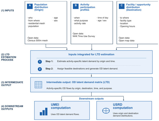
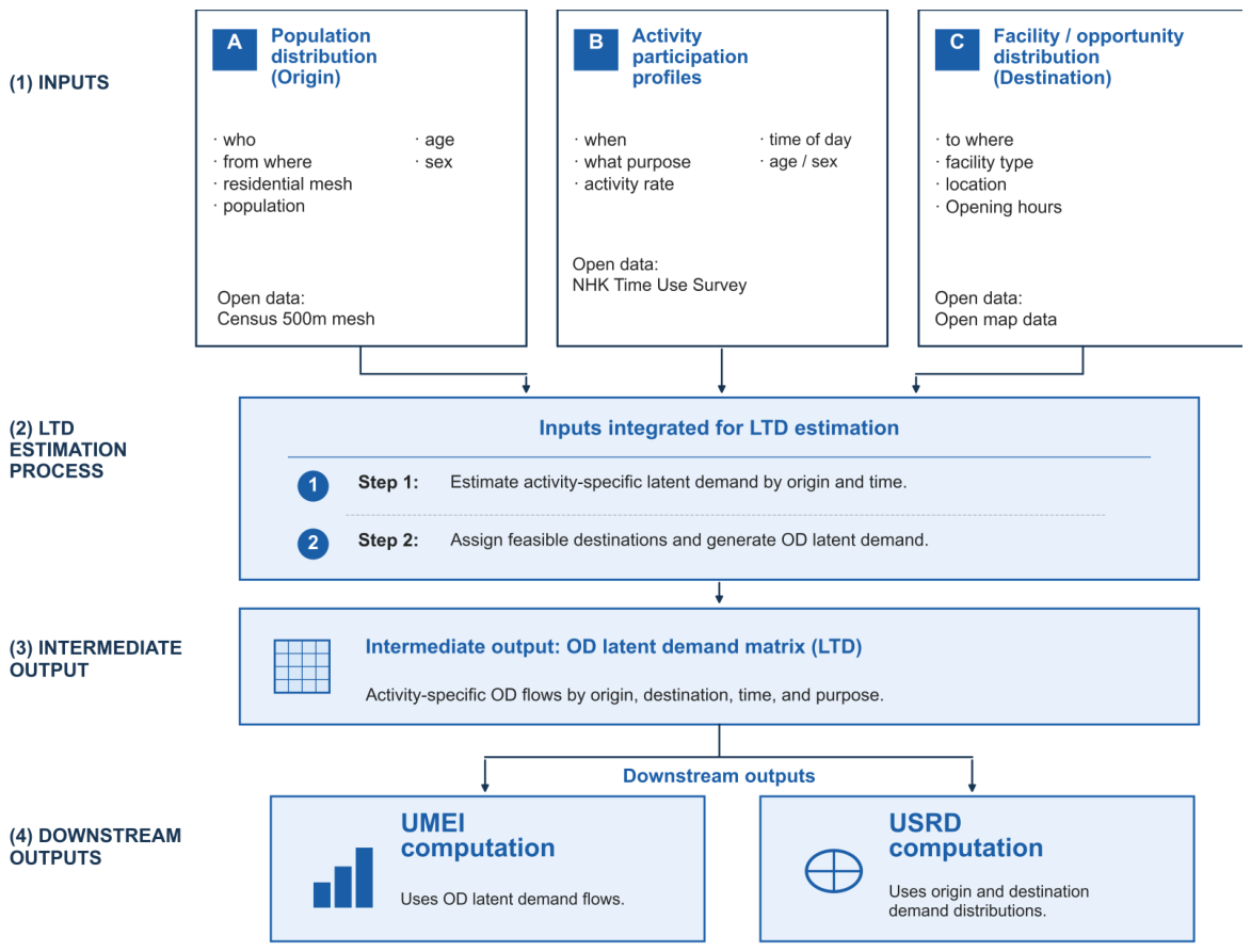
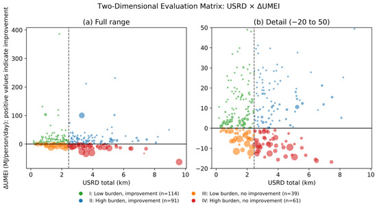
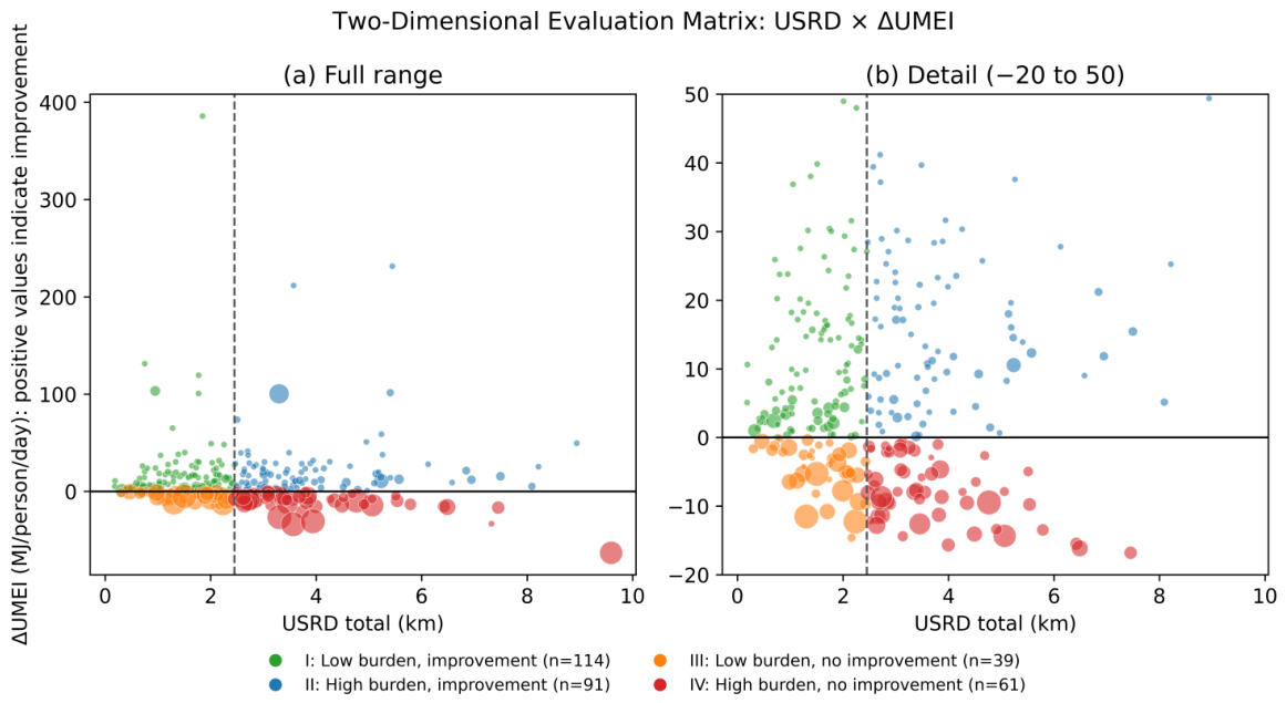
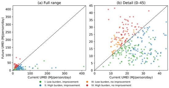
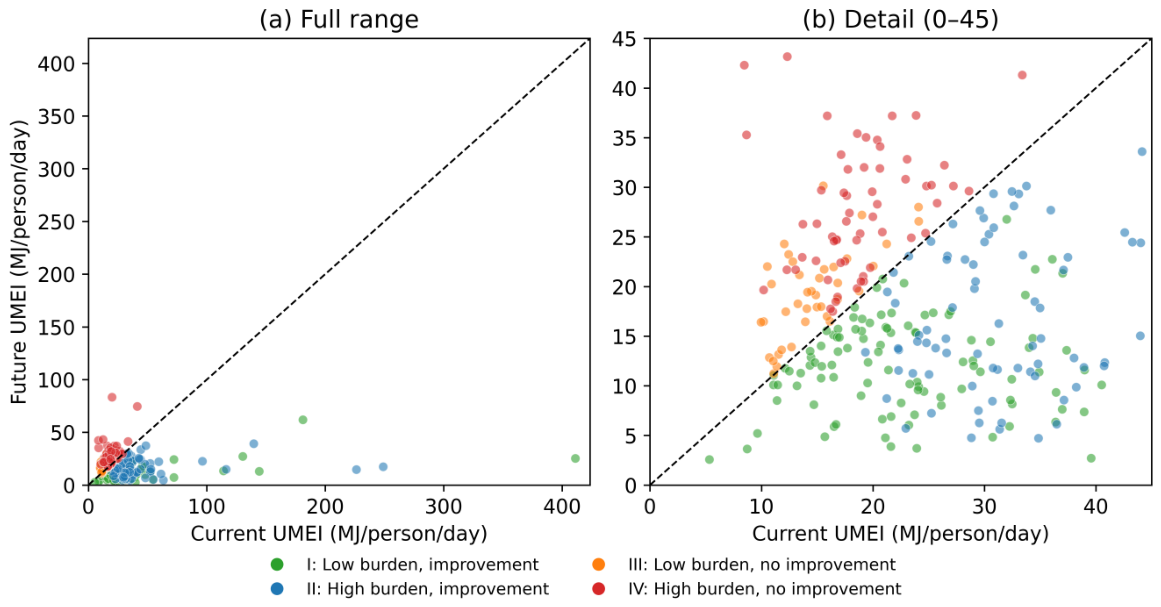
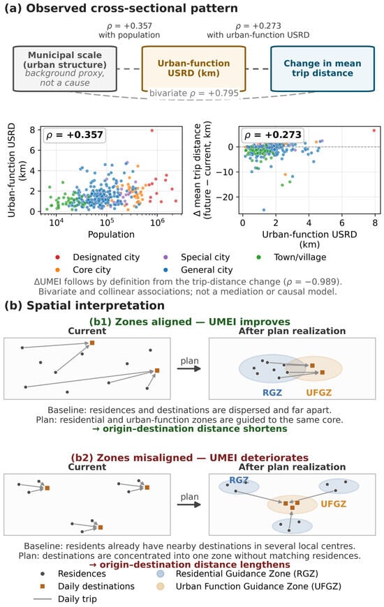
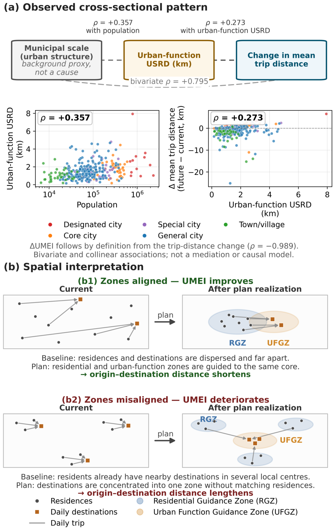

Disclaimer/Publisher’s Note: The statements, opinions and data contained in all publications are solely those of the individual author(s) and contributor(s) and not of MDPI and/or the editor(s). MDPI and/or the editor(s) disclaim responsibility for any injury to people or property resulting from any ideas, methods, instructions or products referred to in the content. |
© 2026 by the author. Licensee MDPI, Basel, Switzerland. This article is an open access article distributed under the terms and conditions of the Creative Commons Attribution (CC BY) license.