


Abstract
Monitoring dynamic post-catastrophic landscapes necessitates unsupervised classification approaches capable of incorporating newly emerging landscape-cover states without relying on predefined classes. Within this framework, the temporal correspondence of independently derived spectral clusters presents a critical methodological challenge. This study compared different temporal correspondence approaches for multi-temporal Sentinel-2 imagery of the post-catastrophic floodplain landscape of Khortytsia Island (Ukraine) from 2021 to 2026. In addition to existing temporal cluster correspondence methods based on centroid distance, Mahalanobis distance, Linear Discriminant Analysis, and Random Forest, geometrically oriented approaches employing the elongation and principal-axis orientation of spectral point clouds were evaluated. A series of tests assessed correspondence accuracy, robustness to seasonal and interannual drift, graph connectivity, and consensus structure among different temporal correspondence solutions. The results demonstrated that geometrically oriented approaches preserved temporal correspondence among landscape-cover states with high stability despite phenological and interannual variability. In particular, axis-based correspondence more effectively maintained separation between corresponding and competing clusters amid progressive temporal divergence. Consensus analysis revealed that disagreement among methods was concentrated in ecotonal and actively transforming zones, indicating areas of increased landscape instability. This study shows that the geometry of spectral trajectories contains valuable information for temporal correspondence and provides a promising foundation for monitoring dynamic post-catastrophic landscape systems.
1. Introduction
Remote sensing provides an effective basis for monitoring landscape and vegetation-cover dynamics, especially in territories affected by ecological catastrophes. Under such conditions, ecosystems may undergo rapid, large-scale, and nonlinear transformations involving changes in species composition, vegetation productivity, habitat structure, and the spatial organisation of landscape cover [1,2]. Therefore, post-catastrophic monitoring requires approaches that can document the current state of the landscape and track trajectories of change, including their intensity, spatial heterogeneity, and temporal persistence [3,4]. In territories affected by ecological catastrophes, it is essential both to document the state of the area at a given moment in time and to track trajectories of change, their intensity, spatial heterogeneity, and temporal persistence [5]. Remote sensing is an effective tool for analysing the spatiotemporal dynamics of landscape and vegetation cover, because it enables the assessment of temporal changes in spatial patterns over large areas, ensures repeatability of observations, and provides a basis for comparing the state of landscape and vegetation cover before, during, and after the impact of destabilising factors [6].
The spatiotemporal dynamics of landscape and vegetation cover can be investigated using continuous spectral-index values, which reflect gradients of surface condition, productivity, or moisture, and classified land-cover categories, which enable the distinction of cover types and the analysis of their spatial relationships [7,8]. While continuous spectral-index values are well suited to capturing gradual changes in the intensity of individual properties [7,9], classified categories provide an interpretation of structural transformations within a territory through changes in cover composition and spatial configuration [10,11]. Obtaining classifications for individual dates and ensuring their accurate comparability over time is critically important. This challenge is addressed through temporal correspondence, which harmonises classification results obtained at different observation dates based on phenological, seasonal, and image-acquisition conditions [12,13]. The necessity of temporal correspondence of land-surface classification results stems from the fact that remote sensing data reflect the class of an object and its state at a specific moment in the seasonal cycle [14]. The spectral responses exhibit significant variation across the distinct phenological phases within vegetation cover [15]. The same vegetation type may appear as different classes on different dates, while different vegetation types may, during certain periods of the year, become spectrally similar [8,16]. These effects are further compounded by variations in moisture conditions, inundation, weather, cloud cover, acquisition geometry, and sensor characteristics, leading to the accuracy of single-date classifications depending strongly on the acquisition date [17,18]. Maps produced for different seasons, years, or satellite platforms may differ not because of actual landscape change but because of differences in observation times, creating a risk of pseudo-change, reducing model transferability, and complicating the accurate comparison of spatiotemporal series [13,19,20]. The temporal harmonisation of land-surface classification results is therefore a necessary condition for reliable monitoring, the detection of genuine cover changes, and the construction of comparable multi-year classifications [12,21].
During the temporal correspondence of land-surface classification results, several challenges are typically encountered. The phenological non-stationarity of vegetation types means that the same vegetation type may exhibit different spectral responses at different phases of the seasonal cycle. Classes that are well separated on one date may overlap on another. In many studies, accounting for phenological dynamics is regarded as an essential component of establishing correspondence among multi-date classifications [21,22,23]. Even in the absence of real change, spectral differences between scenes may arise from atmospheric conditions, illumination, acquisition geometry, and sensor differences. Consequently, inter-date differences often reflect variations in observation conditions rather than actual cover transformation, making reflectance normalisation a critical step before establishing correspondence [24,25]. Even slight misregistration between scenes alters the configuration of object boundaries and may generate false changes, especially along the contours of fine-grained or mosaic landscapes. Although object-based approaches are less sensitive to misregistration, precise co-registration remains essential [26,27]. Reference samples are often derived from field descriptions, thematic maps, or aerial photographs acquired on different dates, under different phenological conditions, or at different spatial resolutions. This introduces label noise into the training data, associated with misregistration, delayed updating, and the intrinsic complexity of the cover itself [28]. Such errors affect both classifier training and validation procedures [29]. Errors also arise from mismatches in resolution and semantic inconsistencies when older, coarser-resolution maps are used for correspondence or as training labels for newer, more detailed products. This issue is particularly important when comparing classifications produced by different sensors or by different generations of mapping products [30]. A further challenge is the methodological incomparability of classifications produced in different years: changes in interpretation rules, spatial detail, feature sets, processing algorithms, and legend structure may generate discrepancies between maps that are unrelated to real cover change. Consequently, part of the detected dynamics may represent an artefact of differences in mapping procedures rather than actual transformation of landscapes or vegetation [31].
Robinson et al. [32] proposed the Temporal Cluster Matching (TCM) framework for detecting temporal changes in structures by comparing spectral cluster distributions inside and outside known object footprints. Although the term “cluster matching” is used in that study, its objective differs fundamentally from the present work. Here, we address the problem of establishing temporal correspondence between independently derived spectral clusters representing landscape-cover states across multi-temporal image series. In object-based pasture mapping, temporal correspondence can be established by matching pasture objects according to the similarity of their multivariate Sentinel-2 time-series trajectories, particularly using Dynamic Time Warping to account for shifts in phenological timing [33]. Correspondence approaches have also been used to analyse spatial correspondence between pixel-based remote-sensing classifications and polygon-based forest inventory maps [34]. Existing correspondence approaches in remote sensing include temporal correspondence of spectral trajectories, object-based correspondence analysis, and hierarchical reconciliation between heterogeneous land-cover representations [35]. In forest monitoring, temporal correspondence can be formulated as the correspondence between abrupt shifts in NDVI time series and specific management events, such as clear-cuts or partial forest cuts [36]. For dynamic landscape monitoring, correspondence may be based on repeated image-pattern correspondence, allowing displacement or trajectory information to be extracted from temporally separated satellite scenes [37]. The use of multi-temporal Sentinel-2 imagery improved vegetation classification accuracy because seasonal phenological changes provided additional discriminatory information between spectrally similar vegetation types [38]. Thus, despite the broad use of correspondence in remote sensing, there remains a methodological gap in temporally linking independently derived vegetation or habitat clusters across multitemporal image series under phenological and interannual spectral drift. This is the problem addressed in the present study.
Phenological and successional dynamics operate on different temporal scales under normal conditions [39]. Phenological changes reflect intra-annual variability in the state of vegetation cover, whereas successional changes characterise the longer-term reorganisation of its structure and composition [40]. However, under catastrophic impacts, the issue of temporal alignment becomes considerably more complex, as these two types of dynamics begin to overlap [38] partially. Following environmental disturbance, phenological variability may manifest as quantitative changes in the spatial proportions of qualitatively similar cover types, where their density, productivity, or degree of development changes without a distinct transition to another type [41]. Catastrophic processes may sharply accelerate successional transformations, so that a qualitative reorganisation of the cover accompanies quantitative changes–that is, a transition to other vegetation types or forms of landscape organisation [42]. Under conditions of ecological catastrophe, interpreting remote-sensing time series requires distinguishing short-term phenological variability from accelerated successional change, because spectrally or structurally similar shifts may have fundamentally different ecological origins.
Temporal changes alter the spectral signatures of the same land-cover objects, making independently generated spectral clusters from different dates inconsistent and therefore difficult to compare directly. Consequently, reliable temporal correspondence between spectral clusters becomes a prerequisite for analysing post-disturbance vegetation dynamics [14]. Our hypothesis is that temporal correspondence between spectral clusters representing the same landscape-cover type can be established from the internal geometry of spectral point clouds, particularly from their elongation and principal-axis orientation in spectral space. This hypothesis is based on the fact that, even within a single observation date, individual patches of the same landscape-cover type may occupy different phenological or successional states. Such within-type heterogeneity produces elongated spectral spectral point clouds whose dominant orientation reflects the principal direction of internal spectral variability. Through time, successive states of the same landscape-cover type form a continuous spectral trajectory that, because of the discrete character of remote-sensing observations, appears as a sequence of partially separated elongated clouds. Under these conditions, the local geometry of a spectral point cloud constrains the probable direction of its subsequent displacement in spectral space and therefore provides a basis for temporal correspondence between successive states of the same landscape-cover type. This geometrically oriented approach is then compared with different temporal correspondence methods, including centroid distance, Mahalanobis distance, Linear Discriminant Analysis, and Random Forest, in order to evaluate whether the geometry of spectral point clouds provides additional information for preserving temporal correspondence among landscape-cover states.
2. Materials and Methods
2.1. Study Area as a Model Landscape System
The floodplain ecosystems of Khortytsia Island on the Dnipro River were selected as the model study area, as they represent a dynamic landscape system that has undergone pronounced post-catastrophic restructuring following the destruction of the Kakhovka Reservoir in 2023 [43] (Figure 1). Khortytsia is the largest island on the Dnipro River, located within the city of Zaporizhzhia, Ukraine, downstream of the Dnipro Hydroelectric Power Plant [44].
Figure 1.
The cascade of reservoirs on the Dnipro River and the location and digital model of the Khortytsia Island. The blue quadrangle on the digital model of the island indicates the study area.
Before the catastrophe, the island was connected with the northern part of the former Kakhovka Reservoir water area and its floodplain–riparian zone [45]. The study covered the period from 2021 to the most recent available satellite observations, which made it possible to compare the state of the landscape and vegetation cover before the catastrophe, during the phase of abrupt hydrological restructuring, and throughout subsequent post-catastrophic development [43]. Following the destruction of the Kakhovka Hydroelectric Power Plant dam on 6 June 2023, the rapid decline in water level caused substantial changes in the hydrological regime, shoreline morphology, moisture conditions of floodplain soils, and the spatial structure of habitats [43,44,46,47]. Within the floodplain system of Khortytsia, these processes were manifested in the disconnection of some water bodies from the main channel, shallowing, exposure of bottom substrates, formation of new sandy shores and shoals, and rapid colonisation of newly exposed surfaces by pioneer and riparian-aquatic vegetation. At the same time, changes in relatively elevated parts of the floodplain may proceed more slowly, but remain ecologically significant because of changes in the moisture regime of the root zone and increased summer stress on woody stands [48,49]. Khortytsia is therefore a suitable model site for analysing the temporal dynamics of landscape cover, as it combines sharply transformed, transitional, and relatively stable areas. This mosaic structure provides conditions for testing remote-sensing methods capable of tracking both gradual changes in known habitat types and the emergence of new, previously unrepresented cover classes [50].
2.2. Acquisition and Primary Processing of Satellite Imagery
A multi-date series of Sentinel-2 MSI (Multispectral Instrument) Level-2A satellite images acquired during 2021–2026 was used for the analysis [51]. Only scenes with low cloud contamination were included in the processing, with total cloud cover not exceeding 5%. Each scene was processed separately within the study-area polygon. Spectral bands were extracted from SAFE archives, clipped to the study area, masked by the polygon boundary, and aligned to a common spatial grid with an identical coordinate reference system, spatial extent, and resolution. The radiometric harmonisation of the imagery was performed, including BRDF (Bidirectional Reflectance Distribution Function) correction to reduce inter-date differences associated with varying acquisition conditions, aimed at reducing the influence of sun–sensor geometry on surface reflectance [52]. Cloud- and shadow-affected pixels were subsequently masked using Sentinel-2 quality layers. To preserve the continuity of the multi-date series, missing values were later reconstructed along the temporal trajectory of each pixel using regression-interpolation gap filling based on neighbouring observation dates [53,54]. Based on the spectral bands, 36 spectral indices were calculated for each date. These indices characterised different aspects of surface condition, including greenness, moisture, vegetation structure, hydrological regime, soil exposure, and integrated spectral brightness components. The formulas of the indices and their ecological interpretation are provided in our dataset [55]. All index layers were geometrically harmonised across dates and aligned to a common raster structure.
2.3. Identification of EUNIS (European Nature Information System) Habitats Based on Plant Communities
Geobotanical surveys, vegetation physiognomy, and the landscape position of patches were used for the interpretation of spectral classes in terms of EUNIS (European Nature Information System) habitats (Table S1). Habitat identification was primarily based on plant associations established from field relevés (Figure S1), whereas vegetation physiognomy, moisture conditions, relief, and spatial context were used as complementary criteria (Table S2). This approach follows the general logic of the EUNIS classification system, in which habitat types are associated with vegetation but are not direct equivalents of phytosociological syntaxa, as their delimitation also depends on ecological and geographical context [56]. The assignment of spectral classes to habitat types was performed by analysing the dominant and accompanying plant associations recorded within each class. This allowed avoiding a rigid “one class–one habitat” correspondence and retaining several spectrally distinct classes within the same EUNIS habitat type when they represented different structural or phenological states of the same habitat. The relationship between spectral classes and plant associations was evaluated using contingency-table analysis [57]. A contingency matrix was constructed in which rows corresponded to plant associations and columns to spectral classes. The overall strength of association was assessed using Pearson’s χ2 test with a Monte Carlo permutation procedure because of the presence of low expected frequencies in part of the matrix [58,59]. The strength of association was quantified using Cramér’s V. Individual classes were additionally evaluated using one-versus-rest comparisons with Holm correction for multiple testing [60,61]. Standardised residuals were used to identify associations that were statistically overrepresented or underrepresented within particular spectral classes [62,63].
2.4. General Study Design and Strategy for Evaluating Temporal Correspondence Methods
The study aimed to evaluate the extent to which different temporal-correspondence methods can preserve the identity of habitat types across a multi-date series of satellite images. Because independently generated clusters cannot be directly compared across dates, the central task is to establish reliable temporal correspondence between clusters representing the same landscape-cover type despite seasonal and interannual spectral variability [14]. The overall analytical framework combined two complementary evaluation modes: a quasi-supervised mode, in which habitat types were defined based on reference geobotanical surveys, and an unsupervised temporal correspondence mode, in which the ability of the methods to maintain a stable cluster structure without direct use of external labels for each date was assessed. In the quasi-supervised mode, reference habitat types were identified for a fixed period of field surveys, after which the quality of their recognition was evaluated when transferring these correspondences to other dates within the satellite time series. This approach enabled assessment of the “ageing” effect of reference information, i.e., the decline in the reliability of correspondences with increasing phenological or interannual divergence from the survey date. In the unsupervised mode, methods were compared based on how consistently they reproduced the temporal continuity of clusters across consecutive dates. This evaluation included the emergence of new codes, the stability of chains of correspondences, the structure of cluster-transition graphs, and the consistency of the resulting superclusters among different temporal correspondence methods.
The methodological workflow consisted of four consecutive stages. First, spectral clusters were generated independently for each observation date. Second, different temporal correspondence methods were applied to establish correspondences among clusters across dates. Third, the resulting correspondences were evaluated using complementary quasi-supervised and unsupervised criteria. Finally, the temporal consistency of the resulting landscape trajectories was compared among methods. This sequential workflow links each methodological component directly to the overall objective of preserving temporal correspondence among landscape-cover states.
2.5. Feature Space for Temporal Correspondence
This step was necessary to ensure that clusters obtained from different dates were compared within the same feature space rather than within date-specific spectral coordinate systems. Because seasonal variation may shift all observations in a similar direction and obscure correspondence among habitat types, the feature space was constructed to reduce the dominant seasonal component while preserving residual differences relevant to temporal correspondence. The purpose of this procedure was not to classify land cover directly, but to create a common spectral reference system in which the geometry, position, and trajectories of clusters could be compared across dates. Calculations were performed in a common ordination space constructed for the full set of observations from all dates, using spectral indices shared by all temporal slices. For each spectral index , the seasonal component was described using a cyclic GAM:
where is the day of year for the -th observation, is a cyclic smooth function, and is the residual component. The residuals were used as seasonally adjusted values. For each date , the robust centre of feature was then calculated as either the median or the trimmed mean:
The values were subsequently centred as:
Within each “class × date” combination, quantile trimming was then applied. Observations were retained if:
where and are the lower and upper quantiles for feature in group on date , respectively. In the analysis, was used. This sequence of transformations produced a comparable set of features for constructing the common correspondence space.
The prepared observations from all dates were analysed in a unified ordination space using a two-step principal component approach. First, principal component analysis of the total spectral variability (hereafter, total PCA) was applied to the complete multi-date dataset. This step extracted the dominant gradients shared across all dates, which for vegetation cover mainly reflected broad variation in greenness, moisture conditions, and surface brightness. In the second step, principal component analysis of residual variation (hereafter, residual PCA, or rPCA) was applied after removing the variation explained by the dominant total PCA gradients. This step was used because the strongest common gradients may mask weaker, but ecologically meaningful, differences among habitat states. The residual components, therefore, represented supplementary spectral structure that was less expressed in the main axes but could be important for distinguishing temporal trajectories and spectrally similar habitat states. Each observation was then represented by its coordinates in this combined component space. All component coordinates were used in the correspondence procedures, while the first two total PCA coordinates were also used to visualise spectral clouds and temporal trajectories.
2.6. Geometric Properties of Spectral Clusters
This section explains why cluster shape, axis orientation, and relative position were used as geometric indicators of temporal continuity between landscape-cover states. The geometric approach was based on the assumption that the shape of a spectral cluster reflects the temporal trajectory of change in the corresponding cover type. Accordingly, the geometry of the cluster can be interpreted as an indicator of the direction of subsequent spectral change and used to establish correspondences between clusters on consecutive dates. Temporal correspondence was therefore based on the shapes of spectral clusters, the orientations of their principal axes, and their relative positions in the common ordination space (Figure 2).
Figure 2.
Schematic representation of geometric correspondence between spectral clusters. The upper panel illustrates the spatial component of the method: for the reference cluster on the previous date (reference), the transverse gap between its axial region and the cluster on the current date is evaluated both for the within-class correspondence (within-class, ) and for the nearest between-class difference (between-class, ). denotes the perpendicular deviation of the centroid of the different cluster from the principal axis of the reference cluster. The lower panel illustrates the angular component of the method, i.e., comparison of the angle between the principal axes of the reference cluster and either the within-class cluster () or the between-class cluster (). Geometric correspondence is based on the assumption that, for the true within-class correspondence, both the transverse gap and the angular mismatch are smaller than for between-class competing clusters.
For each “class × date ” combination, the spectral cluster in the common ordination space was described by a robust geometric descriptor:
where is the robust centroid of the cluster, is the unit vector of the first principal axis, and are the first and second eigenvalues of the robust covariance matrix, and:
is the elongation, or anisotropy, index of the cluster.
The cluster centre and covariance structure were estimated robustly using the minimum covariance determinant method, followed by eigen decomposition of the covariance matrix. The first eigenvector defined the dominant direction of within-cluster variability, whereas the eigenvalue ratio () quantified cluster elongation.
Temporal correspondence was established asymmetrically by comparing each cluster on the current date with all reference clusters from the preceding date. For each candidate pair, the displacement vector between cluster centroids was calculated as:
Its projection onto the principal axis of the reference cluster was defined as:
whereas the perpendicular component was calculated as:
The transverse separation between clusters was then described by the Euclidean length of this perpendicular component:
Thus, represents the longitudinal displacement along the principal axis of the reference cluster, whereas represents the transverse deviation of the centroid of the current cluster from this axis.
For geometric interpretation, an axial “tube” region was defined around the principal axis of each cluster. For the reference cluster, its transverse radius was defined as:
where is the radius scaling coefficient and is the axial expansion parameter. For the current cluster, the transverse radius was defined as:
In the calculations, and were used. Under this setting, the axial region was effectively cylindrical, i.e., its transverse radius did not depend on longitudinal displacement.
The unnormalised transverse gap between two clusters was defined as:
and the normalised transverse gap as:
where is a small positive constant introduced to avoid division by zero. If
the clusters were considered to overlap or touch geometrically in the transverse direction.
The angular difference between the orientations of two clusters was evaluated using their first principal axes:
The integrated geometric similarity score between clusters was defined as:
where and are the weights of the angular and spatial components, respectively.
In the analysis, equal weights were used:
For each cluster on date , the best match on the previous date was defined as the cluster for which was minimal:
where is the set of all clusters present on the previous date. This integrated score was subsequently used as the combined score.
Within-class temporal pairs were compared with their nearest between-class competing clusters from the previous date using angular mismatch , normalised transverse gap , and combined score :
For each within-class pair, the following logical criteria were then recorded:
where is the indicator function.
The separation margin between the true within-class correspondence and the nearest external class was described as:
The geometric criterion was evaluated nonparametrically. Within-class values of , , and were compared with the corresponding nearest between-class competing clusters using one-sided paired Wilcoxon tests. The margin score was tested against zero using a one-sample Wilcoxon test. Geometric connectivity was additionally quantified as the proportion of within-class pairs with overlapping axial regions .
2.7. Axis–Distance and Geometric Methods
The two proposed geometric correspondence methods compare clusters as oriented structures described by their centre, principal-axis direction, and transverse width. The axis–distance method uses only the deviation of a current cluster from the principal axis of a reference cluster, whereas the geometric method additionally incorporates angular alignment and transverse overlap between axial regions. The following cluster descriptor was used as the basic reference for comparison:
where is the centroid of the reference cluster, is the unit vector of its first principal axis, and and are the first and second eigenvalues of the robust covariance matrix.
In the simplest centroid-based variant, correspondence between clusters was established only by the Euclidean distance between their centroids:
The best match for cluster on date was then defined as:
where is the set of all clusters present on the previous date.
The axis–distance method represents a geometric extension of this approach. Here, the reference for comparison is not a single point but the principal axis of the reference cluster, defined by the line:
Unlike a centroid, this axis may pass both through and beyond the spectral point cloud; it therefore represents not only the current state of the system but also the dominant direction of its internal variability, which can be interpreted as a hypothetical trajectory of subsequent spectral change. For a pair consisting of reference cluster at and current cluster at , the centroid displacement vector was calculated as:
with its longitudinal projection onto the principal axis of the reference cluster given by:
and its perpendicular component by:
The axis–distance score was defined as the transverse distance from the centroid of the current cluster to the principal axis of the reference cluster:
Accordingly, the best match was defined as:
The geometric method used the same axial principle but complemented it by assessing the angular alignment of the principal axes and the transverse gap between the axial regions of the two clusters. For this purpose, a transverse radius was defined around the principal axis of the reference cluster as:
and, for the current cluster, as:
where is the scale of the transverse radius and is the parameter controlling expansion along the axis. In the calculations, and were used; therefore, the axial region was effectively cylindrical.
The transverse gap between the two clusters was defined as:
and its normalised form as:
where is a small positive constant. If , the axial regions of the two clusters were considered to overlap or touch in the transverse direction.
The angular mismatch between the principal axes of the two clusters was calculated as:
a quantity ranging from 0 to 1 and independent of the sign of the eigenvector. The integrated geometric score was then defined as:
where and are the weighting coefficients of the angular and spatial components, respectively. In the calculations, and were used. The best match for cluster on date was defined as:
Thus, the axis–distance and geometric methods represent two hierarchically related levels of geometric correspondence: the former uses transverse deviation from the reference principal axis, whereas the latter extends this criterion by incorporating angular alignment and transverse overlap between axial regions.
2.8. Different Temporal Correspondence Methods
This section defines the reference temporal correspondence methods used to benchmark the proposed geometric correspondence approach against established distance-based and classification-based methods. For comparison with the geometric method, four methods for establishing temporal correspondence between clusters on consecutive dates were used: centroid distance, Mahalanobis distance, Linear Discriminant Analysis (LDA), and Random Forest (RF) [32]. All methods evaluated how a cluster on date corresponded to the classes defined on the preceding date , after which the class with the best score was selected. In the centroid method, the Euclidean distance was calculated between the centroid of the cluster on date and the centroids of all reference clusters on date . The class with the minimum distance was considered the best match. The Mahalanobis method used both the centroid and the cluster’s covariance structure. For each class on the reference date, a distributional model was constructed, and for the query cluster, the median Mahalanobis distance of its points to this model was calculated. The class with the minimum distance was then selected as the best match. Linear Discriminant Analysis (LDA) and Random Forest (RF) were used as classification-based methods. These models were trained on points from the reference date. For the points belonging to a cluster on date (lower index 2) , posterior probabilities of membership in each reference class were then obtained. These probabilities were averaged across all points within the query cluster, and the class with the highest mean probability was taken as the corresponding class. The comparison involved the geometric axis-tube method against centroid distance, Mahalanobis distance, LDA, and RF.
Because the complete set of spatial outputs is too extensive to be presented within a conventional journal article, all classification products have been deposited in an accompanying Zenodo repository [64]. The archive contains, for each temporal correspondence method and each Sentinel-2 acquisition date, both georeferenced GeoTIFF rasters and rendered image versions of the resulting classifications. It includes the primary cluster classifications, the corresponding supercluster maps obtained after temporal integration, and the associated spatial products generated throughout the analytical workflow. These materials provide full spatial documentation of the classification results and enable independent verification, visual inspection, and reuse of the proposed methodology.
2.9. Strategy for Comparing Temporal Correspondence Methods for Spectral Clusters
The comparison of temporal correspondence methods for spectral clusters was performed in three consecutive stages (Table 1). In the first stage, the geometric assumption underlying the axis–distance and geometric approaches was tested. Whether spectral point clouds of the same class on neighbouring dates preserve geometric connectivity, that is, whether their orientational and spatial similarity is greater than that of the nearest between-class competing clusters. To this end, the relative position, direction of the principal axis, and degree of overlap of spectral clusters were evaluated in the common ordination space. In the second stage, the practical quality of correspondence between neighbouring dates was assessed. The axis–distance and geometric approaches were compared with different methods based on centroid distance, Mahalanobis distance, Linear Discriminant Analysis, and Random Forest. The comparison was performed in a quasi-supervised mode, in which habitat types were defined from reference geobotanical surveys conducted at a fixed date, after which the transferability of these correspondences to other temporal slices was analysed. In the third stage, the temporal stability of the methods was analysed, that is, changes in correspondence quality with increasing phenological and interannual drift relative to the reference period. The analysis evaluated how rapidly identification accuracy degraded with increasing temporal distance and whether geometrically oriented approaches were better able to preserve correspondence with the true class under conditions of post-catastrophic landscape cover restructuring. The evaluation scheme comprised three interconnected levels: testing the geometric hypothesis, benchmark comparison of practical correspondence quality, and analysis of the temporal stability of different methods.
Table 1.
Criteria and stages for evaluating the axis–distance and geometric correspondence methods.
2.10. Criteria for Comparing Different Temporal Correspondence Methods
The comparison of different temporal correspondence methods between neighbouring dates was performed in a benchmark mode, in which, for each cluster on the current date, , its correspondence to all candidate clusters present on the previous date was evaluated. The true correspondence was defined as the cluster belonging to the same reference habitat class on the previous date. For each correspondence case, the predicted class, the rank of the true class among all candidates (), the indicator for a correct top-ranked correspondence, and the representing the separation between the true class and the nearest competing candidate were determined. The overall performance of the methods was evaluated using top-1 and top-3 accuracy, the mean and median ranks of the true class, and the mean and median values of margin. These metrics were calculated for the full set of transitions between neighbouring dates, as well as separately for each date pair and for each class. For methods based on distance or geometric scores, the best correspondence was defined as the candidate with the minimum score, whereas for Linear Discriminant Analysis (LDA) and Random Forest, the best correspondence was defined as the class with the highest mean posterior probability.
2.11. Evaluation of the Sensitivity of Correspondence Methods to Phenological and Interannual Temporal Drift
This section evaluates whether correspondence methods remain reliable when spectral signatures diverge from the reference survey period because of within-year phenological change and interannual variability. Cluster correspondence across consecutive dates was considered a problem of establishing temporal invariance of vegetation types relative to the reference surveys conducted in August 2024 and 2025. The rationale for this approach was that a reference survey captures the state of vegetation cover at a specific point in time, whereas before and after this date the spectral structure of the same vegetation type changes systematically with seasonal phenology and interannual variability. Accordingly, the comparison of correspondence methods was aimed at evaluating the extent to which each approach preserves the correspondence between clusters of the same type over time under conditions of such drift. The sensitivity of correspondence methods to temporal drift was analysed separately in two aspects. The first aspect, represented by within-year phenological variability, was defined as the distance between the satellite observation date and the reference survey date of the corresponding year. For each observation associated with survey year i, the reference centre was defined as:
that is, 15 August 2024 or 15 August 2025, depending on the value of . Geobotanical surveys were conducted in August 2024 and 2025, and the reference date was conventionally set to 15 August. For an observation acquired on date i, the signed and absolute temporal offsets were then calculated as:
where is the date of the -th satellite observation, is the reference date corresponding to 15 August of the calendar year to which the observation belongs, is the signed temporal offset in days, and is its absolute magnitude. At the level of each “class × date” combination, these values were summarised using the mean and median.
The second aspect represented the interannual component of variability. It was defined as the absolute difference between the year of the satellite observation and the modal year of the reference geobotanical surveys forming the corresponding “class × date” combination. In addition, the number of represented years, as well as the minimum, maximum, and modal survey year, were determined to characterise the composition of the reference dataset. This formulation enabled separating within-year phenological drift from the interannual component of variability. In this way, interannual drift was not an abstract temporal distance but specifically the discrepancy between the image year and the dominant year of the reference material underlying the corresponding cluster. The phenological and interannual drift metrics were subsequently joined to the benchmark results for each date pair. Correspondence quality was evaluated using three indicators: correctness of the top-ranked correspondence, rank of the true class among all candidates, and the margin between the true class and the nearest competing candidate.
For the correctness of the top-ranked correspondence, a generalised linear model (GLM) with a binomial distribution was used. In contrast, linear models (LM) were applied to the log-transformed rank of the true class and to the margin metric. All models included fixed effects of method, the corresponding temporal-drift component, and the interaction between method and drift (method × drift). A statistically significant interaction was interpreted as evidence that sensitivity to temporal drift differs among methods, i.e., that the rate of deterioration in correspondence quality depends on the selected approach. Thus, the analysis tested not only the presence of an overall effect of temporal distance, but also whether its strength varies across correspondence methods. This formulation directly corresponds to the testing strategy defined in the manuscript, in which the key criterion is the interaction .
For phenological drift, separate models were evaluated in which the predictor was the absolute deviation of the image date from 15 August of the same year. For interannual drift, analogous models were fitted using the absolute difference between the image year and the modal year of the reference surveys as the predictor. Within both drift components, comparisons focused on how rapidly increasing temporal distance reduced the probability of correct correspondence, increased the rank of the true class, and altered the margin metric. Slower degradation of these indicators was interpreted as evidence of greater temporal stability of the corresponding method.
2.12. Unsupervised Mode: Temporal Correspondence Without Reference Labels
This section evaluates how consistently different methods establish temporal correspondence when no external reference labels are available. In the unsupervised mode, clustering was performed independently for each date; thus, the resulting clusters initially lacked predefined correspondence across temporal slices. To establish temporal continuity, a global cluster library was constructed sequentially through the time series. Each local cluster identified on the current date was compared with the existing elements of the global library and either absorbed into an existing global code or assigned a new code if no sufficiently similar correspondence was found. This approach avoided forcing newly emerged post-catastrophic surface states into previously existing classes. Temporal correspondence was based on a combined criterion integrating spectral similarity and spatial continuity. Spectral similarity evaluated how closely the current cluster corresponded to previously observed clusters in the common spectral space. In contrast, spatial continuity quantified the extent to which the current cluster occupied areas previously associated with a given global code. If the combined similarity score exceeded a predefined threshold, the cluster inherited the corresponding global code; otherwise, a new global code was created. Consequently, temporal correspondence represented not only changes in spectral properties but also the spatial memory of landscape structure. After construction of the temporal cluster library, the resulting global codes were transferred to the full raster domain. In the present study, this transfer was performed using a Random Forest classifier trained on the cluster library. In contrast, an earlier implementation of the procedure used Linear Discriminant Analysis (LDA) for the same purpose. The classifier was then applied to all pixels for each date, after which the temporal stability of codes, the emergence of new codes, and the structure of superclusters were analysed.
2.13. Identification of Superclusters Based on the Graph of Temporal Correspondences
This section explains how pairwise temporal correspondences were aggregated into graph-based superclusters representing more stable trajectory-level units of landscape cover. A graph of temporal correspondences was constructed to aggregate the primary temporal codes into more stable higher-level units. The vertices of the graph represented the global cluster codes produced during the temporal correspondence procedure, whereas the edges represented recurrent correspondences between codes on consecutive dates. Edge weights characterised the strength of these temporal correspondences. To remove random or weak connections, a minimum edge-weight threshold i.i. (min_edge) was selected in advance by scanning a range of threshold values and identifying the breakpoint beyond which further increases substantially altered the graph structure. After threshold filtering, the graph was partitioned into communities using the Walktrap algorithm [65]. The resulting communities were interpreted as superclusters, i.e., groups of temporal codes that were repeatedly linked throughout the temporal sequence and therefore represented more stable trajectory-level units of landscape cover. Based on the community membership of graph vertices, a correspondence table between the original temporal codes and superclusters was constructed and subsequently used to map and compare methods. To evaluate the structural stability of the superclustering procedure, several integral characteristics of the temporal correspondence graph were additionally analysed, including the number of vertices and edges, graph density, weighted density, graph modularity, the number of connected components, the proportion of the largest connected component, and the entropy of the supercluster distribution. Modularity characterised the strength of graph partitioning into communities, i.e., the degree to which superclusters were separated from one another. The parametric stability of the graph structure was additionally assessed by varying the minimum edge-weight threshold (min_edge) and quantifying its effects on the number of superclusters, graph modularity, and graph connectivity. This enabled the determination of whether the identified superclusters reflected a stable temporal organisation of cluster trajectories rather than artefacts of a particular threshold value.
2.14. Wall-to-Wall Prediction of Cluster Classes and Transfer Quality Assessment
After construction of the cluster library and the correspondence table linking the primary codes to superclusters, classification decisions were transferred from the reference-pixel sample to the full raster for each date. For this purpose, the saved cluster-library object was used, containing the predictor set, standardisation parameters, cluster codes, and the trained classifier. In the present study, the transfer was performed using Random Forest, which was applied to the complete set of pixels for each scene within the same feature space in which the cluster decisions had originally been generated. For each date, a raster map of the primary cluster codes was produced, followed by a supercluster map after application of the correspondence table. In this way, local cluster decisions obtained from the pixel sample were propagated to the entire study area while preserving the consistent temporal numbering of clusters and superclusters. Transfer quality was evaluated through internal validation using the same temporal slices and cluster codes used to construct the cluster library. For each date, the cluster codes generated during the library-construction stage were compared with the codes predicted by the classifier for the corresponding pixels. The overall reliability of transfer was characterised using the mean values and standard deviations of accuracy, balanced accuracy, and macro-F1 [66]. Accuracy represented the overall proportion of correctly reproduced codes, balanced accuracy accounted for unequal class representation, and macro-F1 characterised the balanced quality of recognition across all clusters irrespective of their spatial extent.
2.15. Integration of Temporal Maps into a Spatio-Temporal Model
The series of supercluster maps was integrated into a unified spatio-temporal model to obtain a unified spatial model of landscape dynamics through time and to enable comparison of these dynamics among different temporal correspondence methods. After normalising these values, the relatively dominant supercluster was identified, and surfaces of relative membership were generated, reflecting the proximity of each pixel to the characteristic structure of its corresponding supercluster. At the next stage, contextual superclustering was performed. For each pixel, the local spatial context was evaluated by measuring distances to the nearest patches of different superclusters, and a profile of relative contextual proximity was constructed. Based on these profiles, second-order superclusters were identified, characterised not only by the temporal membership of pixels themselves but also by the similarity of their surrounding spatial context. Additional measures of classification uncertainty were also calculated, including the margin between the nearest competing candidates and the entropy of fuzzy membership. To analyse the dynamics of second-order superclusters, temporal changes in their compositional structure were evaluated. For each supercluster, the proportions of the primary superclusters across different dates were determined, and the contributions of the long-term trend and seasonal components were analysed using partial RDA. Based on the relative importance of the trend and seasonal components, superclusters were classified into seasonal, directional-trend, or mixed-dynamic types.
2.16. Comparison of Supercluster Maps Derived from Different Correspondence Methods
Correspondence among supercluster solutions derived from different correspondence methods was evaluated through the spatial overlap of identically labelled or functionally equivalent superclusters. Because different methods could produce different numbers of superclusters and assign incompatible numerical codes to them, labels were first harmonised relative to the Random Forest reference map. For each supercluster produced by another method, the closest supercluster in the reference map was identified using the maximum Jaccard index. The maps were then compared within this common label system. Based on the harmonised maps, overall agreement among methods was assessed using Fleiss’ kappa [67], pairwise agreement between methods, and the hierarchical structure of method similarity based on the distance . In addition, consensus strength was calculated for each pixel as the proportion of methods assigning that pixel to the dominant harmonised supercluster. This metric was used as a spatial measure of interpretative reliability: high values indicated stable areas reproduced consistently by different methods, whereas low values indicated zones of methodological uncertainty or transitional landscape structure.
The similarity among temporal correspondence methods was additionally visualised using non-metric multidimensional scaling (nMDS) based on the matrix of pairwise Euclidean distances between methods calculated from the standardised evaluation criteria. The resulting ordination was used for graphical interpretation of relationships among methods.
3. Results
3.1. Geometric Structure of Spectral Trajectories
At the level of individual habitat types, temporal changes exhibited an ordered trajectory-like structure within the common ordination space. However, the shape and direction of these trajectories differed substantially among classes (Figure 3). For most habitat types, successive states formed elongated spectral point clouds with a consistent orientation of the principal axis, indicating a pronounced dominant direction of spectral variability.
Figure 3.
Temporal trajectories of spectral point clouds for ten habitat types within the common ordination space. Each facet shows the successive positions of a cluster representing an individual habitat type in the space of the first two components (PC1, PC2). Black points indicate the centroids of spectral point clouds for individual observation dates, grey lines represent temporal transitions between consecutive dates, and blue segments indicate the orientation of the clouds along their first principal axis, i.e., the dominant direction of within-cluster variability.
3.2. Temporal Consistency of Geometric Properties of Spectral Clusters
The geometric criterion of temporal correspondence showed that same-class transitions between neighbouring dates had statistically significantly smaller angles between the principal axes of spectral clusters than the nearest between-class competing clusters (Wilcoxon test, , ). Similarly, the normalised transverse gap between spectral clusters was statistically significantly smaller for within-class pairs than for the nearest between-class pairs (, ). The combined geometric score integrating angular and spatial components was likewise statistically significantly smaller for within-class transitions than for the nearest between-class competing clusters (, ). In addition, margin score values were statistically significantly greater than zero (, ), indicating the presence of a positive separation margin between the true within-class correspondence and the nearest competing class. The distribution of points relative to the equality line showed that, in most cases, within-class temporal pairs had lower combined scores than the nearest between-class competing clusters (Figure 4). This was reflected by the predominance of points above the diagonal. However, the distribution was not homogeneous, with a noticeable proportion of cases below the equality line. The proportion of successful matches according to this criterion was 72.6%, indicating a predominant, although not universal, ability of the geometric approach to correctly distinguish temporally adjacent states of the same class. Consistently, the median value was positive (0.097), and the one-sample Wilcoxon test showed that was statistically significantly greater than zero. The true within-class correspondence tended to have a lower combined score than the nearest between-class difference.
Figure 4.
Comparison of within-class and nearest between-class values of the combined geometric score and the normalised transverse gap (gap norm). The dashed line indicates equality of values; points above this line correspond to cases in which the within-class correspondence had a lower combined score than the nearest between-class difference.
At the level of the normalised transverse gap, within-class temporal pairs in most cases had lower gap norm values than the nearest between-class competing clusters. Such cases accounted for 69.9% of all comparisons, indicating a predominant, although not universal, advantage of within-class correspondences. The median normalised transverse gap for within-class pairs was lower than that of the nearest between-class competing clusters ( versus ), and the paired Wilcoxon test confirmed a statistically significant shift towards smaller within-class values (, ).
Because negative gap norm values in the applied metric correspond to spatial overlap or contact between the axial “tubes”, these results indicate that temporally adjacent states of the same class were, on average, characterised by stronger geometric proximity than the nearest between-class competing clusters. At the same time, the distribution of points was not homogeneous, with approximately 28.3% of cases failing to meet this criterion, indicating a substantial proportion of ambiguous transitions. Among within-class pairs, overlap of the axial regions was observed in 95.3% of cases, further supporting a high, although not absolute, degree of temporal connectivity of spectral clusters in the gap norm feature space.
3.3. Comparison of the Axis–Distance and Geometric Correspondence Methods with Tested Approaches
The Random Forest method achieved the highest top-1 accuracy (0.72) in a benchmark evaluation of six approaches to cluster correspondence between adjacent dates. In contrast, both proposed approaches also demonstrated strong performance: the Geometric method reached a top-1 accuracy of 0.70, and the Axis–distance method achieved 0.68 (Table 2). At the same time, the highest top-3 accuracy was obtained by the Axis–distance method (0.93). In contrast, the Geometric method and Random Forest both showed identical values of 0.92, indicating stable inclusion of the true class among the nearest candidates. Both proposed methods substantially outperformed the Centroid and LDA methods, and especially the Mahalanobis approach. According to ranking-based metrics, the Axis–distance method also occupied one of the leading positions: the median rank of the true class was equal to 1, and the mean rank was 1.65, which was better than those of the Geometric method (1.68), Centroid (1.79), LDA (1.84), and Mahalanobis (2.44), and was surpassed only by Random Forest (1.59). Thus, Random Forest remained the best-performing approach under the strict top-1 accuracy criterion; however, both proposed geometrically oriented approaches demonstrated high competitiveness. The Geometric method achieved nearly maximal top-1 accuracy, whereas the Axis–distance method achieved the best top-3 accuracy and one of the strongest overall ranking performances.
Table 2.
Comparison of different approaches in the benchmark analysis of cluster correspondence between adjacent dates (N queries = 626).
Correspondence accuracy generally increased during the year for all tested methods, from the winter–spring period towards the second half of summer and autumn. However, the pattern of this increase differed substantially among approaches (Figure 5). The largest amplitude of seasonal change was observed for the axis–distance and geometric methods. For axis–distance, predicted top-1 accuracy ranged from 0.315 to 0.840, with an amplitude of 0.525. For the geometric method, the corresponding values were 0.348, 0.872, and 0.524. Random Forest also showed a pronounced seasonal increase, although slightly weaker than that of the two proposed geometrically oriented approaches: predicted accuracy ranged from 0.470 to 0.861, with an amplitude of 0.391. For LDA and centroid distance, the seasonal trajectory was smoother and closer to monotonic: predicted accuracy ranged from 0.346 to 0.727 for LDA and from 0.425 to 0.737 for centroid distance, with amplitudes of 0.380 and 0.311, respectively. The Mahalanobis method showed the lowest accuracy throughout the year, with a predicted range of only 0.265–0.524 and the smallest seasonal amplitude among all methods, 0.259.
Figure 5.
Seasonal dynamics of top-1 accuracy for different correspondence methods between neighbouring dates. Points represent empirical accuracy values for individual date pairs, lines show binomial GAM estimates, and grey bands indicate 95% confidence intervals. Accuracy increased towards the second half of the season for all methods, most markedly for the axis–distance method and Random Forest. In contrast, the Mahalanobis distance maintained the lowest accuracy values throughout the year.
GAM analysis confirmed a statistically significant seasonal trend for all methods. At the same time, the effective degrees of freedom () indicated that the trend shape differed across approaches. For LDA () and centroid distance (), the seasonal relationship was effectively close to linear. For the geometric method () and Random Forest (), moderate nonlinearity was observed. In contrast, the seasonal trajectory was more complex for axis–distance () and especially for Mahalanobis distance (). Thus, the proposed approaches, particularly the axis–distance and geometric methods, showed the most pronounced seasonal restructuring of accuracy, indicating high sensitivity to within-year changes in the spectral structure of vegetation cover. At the same time, Random Forest also achieved high accuracy in the second half of the season. In contrast, centroid distance, LDA, and especially Mahalanobis distance were inferior in both the level and amplitude of the seasonal maximum.
3.4. Correspondence Error Under Increasing Temporal Divergence from the Reference Surveys
For phenological drift, the global effect of temporal distance from the reference date was not statistically significant for the correctness of the top-ranked match. Still, it was statistically significant for the rank of the true class () and for the separation margin between the true class and the nearest competing candidate () (Table 3). The interaction was statistically significant for top-ranked correctness () and separation margin () but was not significant for the rank of the true class (). This indicates that sensitivity to phenological drift differed among methods primarily in the probability of correctly identifying the top-ranked class and the degree of separation between the true class and the nearest competing candidate. In contrast, the rank of the true class showed greater deterioration across methods. For top-ranked correctness, centroid distance showed the highest stability (), followed by Mahalanobis distance () and LDA (), whereas Random Forest (), axis–distance (), and especially the geometric method () exhibited a faster decline in correctness with increasing phenological drift. For the rank of the true class, the slowest rate of deterioration was observed for LDA (), followed by centroid distance () and Random Forest (), whereas axis–distance () and Mahalanobis distance () were slightly less stable. The geometric method () showed the fastest increase in the true class’s rank. For the separation margin, the highest stability was observed for axis–distance (); very similar results were obtained for LDA (), centroid distance (), and Random Forest (), whereas the geometric method () lost separation margin more rapidly. Mahalanobis distance () differed strongly in the direction of the lowest stability. Thus, under phenological drift, axis–distance did not show an advantage in terms of top-ranked correctness or rank of the true class but proved to be the most stable according to the separation-margin criterion, i.e., it best preserved the separation between the true class and the nearest competing candidate. In contrast, the geometric method showed lower phenological stability across all three metrics.
Table 3.
Method profiles for phenological drift.
For interannual drift, the global effect of temporal distance was not statistically significant for the correctness of the top-ranked match. Still, it was clearly expressed for the rank of the true class () and for the separation margin between the true class and the nearest competing candidate () (Table 4). The interaction was likewise not significant for the correctness of the top-ranked match (). Still, it was statistically significant for the rank of the true class () and especially for the separation margin (). This indicates that increasing interannual temporal distance was not associated with a consistent decline in the probability of correct top-ranked correspondence across all methods but was associated with a deterioration in the rank position of the true class and a reduction in its separation from the nearest competing candidate. At the same time, the significant interaction effects for the rank of the true class and the separation margin indicate that sensitivity to interannual drift differed among methods, i.e., that the rate of deterioration in correspondence quality depended on the selected approach. For the rank of the true class, the slowest rate of deterioration was observed for centroid distance (0.01), followed by LDA (0.03), Random Forest (0.04), and axis–distance (0.04), whereas the rank of the true class increased more rapidly for the geometric method (0.05) and especially for Mahalanobis distance (0.07).
Table 4.
Method profiles for interannual drift.
For the separation margin, the axis–distance method showed the highest stability (minus 0.02). Very similar results were obtained with Random Forest (minus 0.03) and LDA (minus ). In contrast, the loss of separation margin was noticeably greater for centroid distance (), even more pronounced for the geometric method (), and extremely strong for Mahalanobis distance (). The axis–distance method combined a relatively moderate deterioration in top-ranked correctness with the highest stability in separation margin, indicating better preservation of the separation between the true class and the nearest competing candidate even under conditions of deterioration in the true class’s rank position.
3.5. Wall-to-Wall Prediction Accuracy for Tested Approaches
The centroid, LDA, and Random Forest approaches show comparable performance, with no pronounced advantages. Detailed confusion matrices for the tested approaches, including class-specific patterns of correct and incorrect assignments, are provided in Supplementary Table S3. Model transfer over the full raster shows similar values of accuracy and balanced accuracy across most approaches, while differences between methods are more clearly expressed in macro-F1 (Table 5). The axis–distance method achieves the highest accuracy and macro-F1 among the tested approaches. In contrast, the Mahalanobis method exhibits lower overall accuracy but higher macro-F1, indicating improved class balance at the expense of overall correctness. The centroid, LDA, and Random Forest approaches show comparable performance, with no pronounced advantages.
Table 5.
Model transfer accuracy over the full raster for temporal correspondence methods.
3.6. Internal Stability of Temporal Correspondence Methods
The internal stability analysis revealed substantial differences among the temporal correspondence methods (Table 6). Random Forest and LDA produced the fewest new codes, indicating the most stable temporal correspondence structure. Axis–distance also showed relatively high stability, with only 32 new codes across 93 dates. In contrast, the Mahalanobis approach generated a markedly higher number of new codes and a much higher mean number per date, indicating strong temporal fragmentation and lower internal stability. The geometric and centroid approaches showed intermediate and very similar behaviour. The results suggest that Mahalanobis distance is the least stable correspondence strategy, whereas Random Forest, LDA, and Axis–distance provide more temporally consistent code propagation.
Table 6.
Internal stability of temporal correspondence methods based on code generation dynamics. All methods were evaluated across 93 dates with 7 final global clusters. The number of codes per date was identical across approaches, with a mean of 9.32, SD of 2.52, range of 5–20, and 95th percentile of 13.4.
3.7. Graph Structure and Robustness of Supercluster Aggregation Among Correspondence Approaches
The supercluster graphs were constructed from recurrent transitions between codes across consecutive dates, reflecting their mutual temporal correspondence (Figure 6). Using a common thresholding rule, these transitions were integrated into a unified correspondence structure, from which the final supercluster grouping was derived. The resulting graphs represent the aggregated correspondence solutions, characterised by specific numbers and configurations of superclusters for each method.
Figure 6.
Supercluster graphs obtained under temporal correspondence methods. Nodes represent temporal codes generated during model transfer, and edges indicate recurrent correspondence links between codes across consecutive dates after thresholding by the selected min_edge value. Node colours denote graph-derived superclusters, while node size reflects the relative contribution or connectivity of each code within the graph. Panels show the graph structures for the tested correspondence approaches: (a) Axis–distance, (b) LDA, (c) spectral ellipse distance, (d) Euclidean, (e) Mahalanobis, and (f) Random Forest. More compact and well-separated graph structures indicate more stable aggregation of temporal codes into superclusters, whereas highly dense or fragmented structures reflect lower stability of temporal correspondence.
The comparative analysis reveals clear differentiation among the evaluated methods in terms of graph structure and parametric robustness, with consistent patterns observed across metrics and their integrated representation (Table 7). The constructed graphs differ markedly in their size, connectivity, and degree of structural organisation, reflecting differences in how temporal correspondences between clusters are aggregated. At the structural level, methods such as Geometric and Centroid produce relatively dense and well-connected graphs, characterised by a small number of components and a high share of nodes concentrated within the largest component. In contrast, Axis–distance, LDA, and Random Forest yield more fragmented structures, with multiple disconnected components and lower largest-component dominance, indicating a more conservative correspondence behaviour.
Table 7.
Graph structure and robustness metrics for different cluster-correspondence methods.
Differences are also evident in modular organisation. LDA exhibits the highest modularity, suggesting clearer separation between superclusters, whereas Centroid shows lower modularity, reflecting less distinct community structure. The number and entropy of superclusters further indicate variation in the distribution of cluster relationships across the graph. The most pronounced contrast is observed for the Mahalanobis approach, which demonstrates extreme behaviour across nearly all metrics. It produces a substantially larger graph with a very high number of nodes and edges, resulting in a fully connected structure (single component) with maximal largest-component share. Despite relatively high modularity, this configuration is associated with excessive connectivity and a lack of structural sparsity, resulting in markedly elevated fragility indices and substantial parameter-dependent variability. These results indicate that methods differ in correspondence accuracy and in the structural properties of the resulting temporal correspondence networks. Approaches such as Axis–distance and Random Forest maintain more fragmented and stable graph structures, whereas Mahalanobis introduces excessive connectivity and reduced robustness under parameter variation.
The ordination provides a more coherent interpretation of these relationships by projecting the multidimensional metric space into a continuous structure, where distances among methods reflect their overall dissimilarity (Figure 7).
Figure 7.
Multidimensional scaling (MDS) ordination of different cluster-correspondence methods based on graph-structure and robustness metrics, with envfit vectors indicating the direction and relative contribution of individual variables. Distance to the ideal solution (integral score): Axis–distance (1.10; 0.48), Centroid (1.74; 0.37), Geometric (2.05; 0.33), Random Forest (2.05; 0.33), LDA (2.45; 0.29), Mahalanobis (3.06; 0.25).
The configuration shows a distinct separation of Mahalanobis along the gradient defined by graph fragility and range-based instability, confirming its deviation from the other methods. In contrast, LDA and Random Forest are aligned with higher modularity and component dominance, indicating a tendency toward more consolidated but less fragmented structures. Axis–distance occupies an intermediate position, without strong alignment with any single metric vector, indicating a balanced trade-off between structural and stability-related properties. This is consistent with its minimal distance to the ideal solution, suggesting that it does not maximise individual metrics but avoids extreme values across the entire set. Centroid and Geometric methods are located near the density-related vectors, reflecting their association with increased edge density and weighted connectivity, while remaining separated from the instability gradients. The orientation of vectors further clarifies the underlying structure of the metric space. Variables related to graph size and connectivity (nodes, edges, component range) form a coherent gradient opposing modularity-related measures, while fragility and variability indicators define an independent axis of instability. The relative positions of the methods along these gradients demonstrate that differences among them arise not from a single dominant property, but from distinct combinations of structural compactness, modular organisation, and robustness.
3.8. Ordination of Graph Structure and Robustness Profiles of Correspondence Methods
The overall agreement among the six different supercluster maps was moderate and statistically significant (Fleiss’ κ = 0.363, z = 1332, p < 0.001). This indicates that the methods reproduced a common spatial structure, although certain discrepancies remained in the assignment of pixels to superclusters. Pairwise comparisons between methods were further visualised using hierarchical clustering based on the distance measure 1—agreement (Figure 8a). This representation allowed the grouping structure among the different classification approaches to be assessed. The resulting dendrogram showed that the two geometric methods, spectral ellipse distance and axis distance, formed the closest pair, whereas Random Forest was the most distinct from the remaining methods.
Figure 8.
Consensus strength and similarity structure of cluster solutions across temporal correspondence methods: (a) hierarchical clustering (dendrogram) of methods based on pairwise agreement, expressed as distance (1 − agreement); (b) the spatial distribution of consensus strength, representing the degree of agreement among methods for each pixel.
Different temporal correspondence methods produced different supercluster solutions, and the relationships among these solutions were quantified using consensus strength. This index describes the proportion of methods that assigned the dominant supercluster label to each pixel. Higher values, therefore, indicate stronger agreement among methods, whereas lower values indicate spatially localised uncertainty in supercluster assignment. The mean consensus strength was 0.612 ± 0.225, with a median of 0.500. The interquartile range was 0.500–0.833, indicating spatial heterogeneity in agreement among the different temporal correspondence methods. Spatial variation in consensus strength was clearly structured by the main geomorphological gradients of the study area (Figure 8b). The highest values were associated with the highest-relief positions and open water surfaces, indicating that these spatial units were consistently identified across different correspondence methods. In contrast, the dynamically changing transitional part of the relief showed substantially lower consensus strength, reflecting bigger method-dependent differences in supercluster assignment. This pattern suggests that disagreement among methods was concentrated mainly in ecotonal and geomorphologically transitional zones, where landscape-cover conditions are more heterogeneous and temporally unstable.
3.9. Spatio-Temporal Consistency of Aligned Supercluster Solutions Across Correspondence Methods
The aligned supercluster solutions showed a generally consistent spatial structure across temporal correspondence methods and reproduced similar temporal patterns. Although the relative areas and model fits varied across methods for individual superclusters, the dominant dynamic types were broadly comparable. Directional trends were repeatedly identified for several superclusters, whereas seasonal or mixed patterns occurred mainly in more transitional units (Table 8). This indicates that the different temporal correspondence methods differed in the precise spatial allocation of some pixels but converged in identifying the major spatiotemporal organisation of the landscape.
Table 8.
Dynamic characteristics of aligned superclusters across temporal correspondence methods (all reported R2 values are statistically significant).
The aligned supercluster maps represent an integrated spatial synthesis of the temporal correspondence methods (Figure 9).
Figure 9.
Spatial distribution of aligned superclusters across temporal correspondence methods. Panels correspond to methods in the following order: (a) Axis–distance, (b) Geometric (spectral ellipse distance), (c) LDA, (d) Centroid (Euclidean), (e) Mahalanobis, and (f) Random Forest. Colours represent harmonised supercluster labels consistent across all maps.
Despite local differences among methods, the resulting spatial patterns remained broadly consistent. They highlighted the same major geomorphological and temporal structures of the landscape. These aligned solutions therefore provide a common analytical framework that can serve as a basis for subsequent quantitative assessments using landscape-ecological approaches, including analyses of spatial heterogeneity, connectivity, ecotonal structure, and temporal landscape dynamics.
4. Discussion
4.1. Temporal Correspondence as a Problem of Continuity in Dynamic Landscapes
Temporal correspondence in satellite image analysis is a complex methodological problem because spectral correspondence between images depends not only on acquisition conditions but also on the temporal variability of the observed landscape system [16,41,68]. The problem of spectral correspondence of satellite imagery encompasses two interrelated dimensions: observational and conceptual. The observational dimension relates to the temporal gap between acquisition dates, during which spectral continuity between images progressively deteriorates [69]. As the interval between observations increases, differences caused by phenological development, moisture conditions, illumination, and other acquisition-related factors may accumulate, altering not only individual spectral values but also the overall configuration of spectral relationships among classes [70,71,72]. Hypothetically, if the temporal resolution of the image series were sufficiently high to render this degradation negligible, different correspondence approaches would be expected to yield similarly high correspondence accuracy. In terms of its observational design, the Sentinel-2 constellation is intended to provide a revisit frequency sufficient for accurate and reliable temporal correspondence, because substantial phenological changes in vegetation cover are generally unlikely to occur within such short intervals. However, meteorological conditions significantly constrain the availability of high-quality, cloud-free imagery, thereby introducing considerable irregularity into the dataset’s effective temporal structure [73,74]. Our image series for 2021–early 2026 confirms this limitation: despite the nominal revisit capacity of Sentinel-2, the effective multi-temporal dataset comprised 93 usable observation dates, with a mean interval of 20.1 days between consecutive images and a median interval of 10 days. The minimum interval was 2 days, whereas the maximum interval reached 100 days. The shortest intervals between high-quality images were most typical in the second half of summer and early autumn, whereas the longest gaps occurred during winter and early spring. This pattern is consistent with the general seasonal availability of usable optical satellite observations in temperate Europe, where cloud-, shadow-, and snow-free observations are unevenly distributed through the year and often require compositing or interpolation to obtain uninterrupted time series [75,76]. Importantly, the most pronounced phenological transitions occur during spring, precisely when the availability of suitable imagery is often at its lowest. This makes temporal correspondence particularly challenging and methodologically relevant under conditions where the continuity of satellite image time series is substantially interrupted.
Gaps between observation dates can be partly compensated for by using observations from other years acquired on similar days of the year, thereby reconstructing an average or expected annual phenological trajectory from multi-year satellite time series [40,75,77]. The calendar year is therefore ignored as an independent temporal dimension. In contrast, the day of the year is used as the primary reference for aligning observations along a common seasonal trajectory [78]. However, under highly dynamic or post-disturbance conditions, interannual variability becomes ecologically significant in its own right. In such systems, combining observations from different years into a single phenological trajectory may obscure abrupt transitions, accelerated succession, and regime shifts. Therefore, unsupervised classification is particularly important for catastrophe-induced dynamic landscapes, as it allows newly emerging surface types to be incorporated without forcing them into predefined classes. Nevertheless, this flexibility does not eliminate the problem of temporal gaps: when the continuity of satellite image series is interrupted, spectral states must still be linked, separated, or registered as new across unevenly spaced observation dates.
A key conceptual issue concerns the landscape unit’s category. Supervised classification implicitly treats landscape units as a priori-defined entities that objectively exist as discrete, identifiable classes [79,80,81]. Although this assumption simplifies reality, it is methodologically convenient and practically useful. However, it also imposes an important limitation: the set of possible system states is effectively treated as fixed. Even if this set can hypothetically be expanded, the spectrum of admissible states remains constrained by prior knowledge and predefined categories. As a result, such an approach leaves little room for genuinely new system states to emerge. For modelling processes in dynamically changing systems, it is essential to retain the ability to identify novel states and incorporate them into the system’s temporal trajectory. In this context, the concept of landscape continuity becomes particularly important [82]. How can relationships between different system states be established through time when the states themselves are changing? One possibility is system stationarity, in which the system largely preserves its properties over time. Another is directional transformation, where change proceeds along one dominant trajectory or several different trajectories. A further possibility is the disappearance of one system and the emergence of another in its place. Under such conditions, a fundamental problem arises: how can one determine whether the original system has merely changed its properties or whether an entirely new system has emerged? This conceptual issue gives rise to the natural spatial heterogeneity of the entity that we identify as a landscape-cover type. In our view, the concept of landscape continuity explains why natural spatial heterogeneity contains the key to resolving the problem of temporal correspondence.
The two complementary criteria were therefore employed for the spatio-temporal correspondence of evolving landscape-cover states: spatial position, which reflects spatial continuity and the inheritance of landscape structure, and spectral similarity, which indicates correspondence in surface properties. Natural processes result from long-term successional dynamics of landscape cover, in which some system states are successively replaced by others, forming ordered sequences of transformations [83]. Catastrophic events of natural or anthropogenic origin may abruptly interrupt such continuity [84]. However, they themselves initiate new chains of interconnected processes, thereby spatially inheriting their effects. For this reason, the spatial criterion is critically important for correspondence procedures. Spectral similarity reflects the qualitative identity of a particular cover type and its distinction from other types. At the same time, spectral properties may change while the system still preserves its qualitative identity. A territory characterised by a specific set of spectral properties, therefore, represents a particular type of landscape cover. Temporal correspondence becomes complicated because both the spatial extent of such cover types and their spectral characteristics are subject to spatial and temporal variability.
4.2. Geometric Interpretation of Spectral Heterogeneity
Our findings support and extend the generalisation proposed by Small and Sousa [85] that land-cover classes should not be treated as compact and internally homogeneous spectral entities, but rather as structured manifolds of admissible spectral states. From the perspective of landscape continuity, asynchronous phenological and successional dynamics within the same cover type produce ordered internal variability [41]. Our results demonstrate that this variability is expressed geometrically as cluster elongation, providing information about the dominant direction of temporal spectral change. Differences in moisture conditions, microrelief, species composition, and disturbance history produce continuous variation among patches. The spectral representation of a landscape-cover type forms an elongated cloud rather than a compact spheroidal one. Under this interpretation, the internal geometry of the spectral point cloud may contain information about the temporal trend of transformation within a landscape-cover type. Our findings support this assumption: the same landscape-cover types form inherited trajectories in spectral space. Even when their typical spectral values change substantially through time, temporally adjacent states tend to remain connected within the same structured manifold rather than shifting to unrelated regions of spectral space.
The principal axis of the spectral point cloud can be regarded as a local trace of the broader trajectory followed by a landscape-cover type in spectral space. It is important to distinguish between the global structure of the spectral space and the local geometry of individual spectral point clouds. The ordination space derived from PCA/rPCA characterises the dominant structure of spectral variability across the entire dataset, whereas the principal axes used in the correspondence procedure are estimated separately for each landscape-cover type and describe the internal geometry of individual spectral clouds within that shared coordinate system. Thus, the directional properties used for correspondence are not imposed directly by the ordination itself but emerge from the organisation of independently formed clusters in the common spectral space. It therefore provides a basis for reconstructing the main direction of landscape-cover transformation across successive temporal states. Similar to ecological trajectories in ordination analysis [86,87], it represents the main gradient of within-cluster variability and therefore approximates the most probable direction of subsequent temporal displacement. This becomes particularly important during phenological and post-disturbance changes. The results of this study indicate that the identity of a landscape-cover type is not always preserved by centroid position alone: even when the centroid shifts substantially, the orientation of the spectral point cloud may retain information about the inherited trajectory of the same type in spectral space. These findings show that temporally adjacent states of the same landscape-cover type may shift substantially in spectral space while their spectral point clouds remain aligned along the same directional trajectory. The preservation of within-class directional similarity indicates that the observed spectral trajectories were not arbitrary but were constrained by the internal structure of the corresponding landscape-cover type.
For clusters belonging to the same landscape-cover type, overlap of axial regions between consecutive dates provides the geometric basis for reliable axis-based correspondence, because temporal correspondence is preserved through inherited alignment along the dominant axis of spectral variability. Ecological systems may undergo substantial spectral shifts without losing their qualitative identity, particularly during seasonal or post-disturbance dynamics [41,88,89]. Under such conditions, centroid-based approaches may interpret directional displacement within the same landscape-cover type as class replacement, whereas geometric overlap preserves information about trajectory inheritance within that cover type. These findings indicate that the predominance of overlap among within-class transitions supports the hypothesis that spectral trajectories retain geometric inheritance across successive states. Conversely, incomplete overlap in some transitions may mark episodes of accelerated restructuring or the emergence of transitional landscape states under post-catastrophic conditions.
The findings of this study provide empirical support for the hypothesis of geometric connectivity among spectral clusters, although this connectivity was not universal across all transitions. Dedicated evaluation of the geometric criterion demonstrated that within-class transitions between neighbouring dates were characterised by smaller angular and spatial differences than the nearest between-class competing clusters, together with a positive separation margin between the true correspondence and the nearest competing class. This confirms that temporally adjacent states of the same class indeed preserve geometric similarity within the common ordination space, and therefore that the shape of the spectral cluster and the orientation of its principal axis can be used as an informative basis for temporal cluster correspondence. In a benchmark comparison of six approaches to cluster correspondence across neighbouring dates, Random Forest achieved the highest top-1 accuracy, although both proposed geometrically oriented approaches also performed well. The geometric method reached near-maximum top-1 accuracy and generally confirmed high practical suitability for correspondence neighbouring temporal states. The axis–distance method was not the best according to the strict top-1 accuracy criterion. Still, it demonstrated the highest top-3 accuracy and one of the best rank-based performances, indicating a stable ability to retain the true class among the nearest candidates. Thus, in practical terms, the proposed methods proved competitive with standard methods, although their strengths differed: the geometric method performed better under the strict first-choice criterion, whereas the axis–distance method showed greater rank stability and a broader margin of correct separation. Drift analysis showed that a single dimension cannot describe the temporal stability of the proposed approaches. For phenological drift, the global effect of temporal distance was significant for the rank of the true class and the separation margin. In contrast, the interaction was significant for top-ranked correctness and separation margin. Under these conditions, the axis–distance method did not show an advantage in terms of top-ranked correctness or rank of the true class. Still, it proved to be the most stable according to the separation-margin criterion, i.e., it best preserved separation between the true class and the nearest competing candidate. In contrast, the geometric method showed lower phenological stability and was inferior to more stable differences across all three metrics. For interannual drift, the global effect of temporal distance was likewise pronounced for the rank of the true class and the separation margin. At the same time, the interaction was significant specifically for these two metrics. In this case, the axis–distance method again demonstrated the highest stability according to the separation-margin criterion. However, for the rank of the true class, it was inferior to centroid distance, LDA, and Random Forest. The geometric method again showed no advantage and, under interannual variability, deteriorated more rapidly than axis–distance, centroid distance, LDA, and Random Forest. The axis–distance method should be interpreted as a structurally oriented and interpretable approach whose main strength lies not in maximising top-ranked correctness under all conditions, but in preserving the geometric identity of the true class and maintaining its separation from competing methods under temporal drift. The geometric method, in turn, is best regarded as an effective benchmark-level approach for short-term correspondence between neighbouring dates but offers little advantage in terms of temporal stability. Overall, both proposed approaches confirmed the value of geometric descriptions of spectral clusters for temporal correspondence tasks. Among interpretable approaches, the axis–distance method proved the most promising when preserving separation between the true class and the nearest competing candidate cluster is of primary importance.
4.3. Why Do the Geometric Method and Axis–Distance Behave Differently?
The comparison of the proposed approaches indicates that the geometric and axis–distance methods should not be interpreted simply as competing methods in which one universally outperforms the other. Instead, they represent two different correspondence regimes based on different assumptions about temporal continuity in spectral space. The geometric method demonstrated high correspondence accuracy for neighbouring dates, indicating that detailed cluster geometry contains substantial information about short-term temporal correspondence. Because the method simultaneously considers cluster orientation, transverse overlap, and local geometric configuration, it is highly sensitive to the fine structure of spectral clouds. This allows precise identification of temporally adjacent states when phenological displacement remains relatively limited. It should be emphasized that the dependence on detailed local geometry makes the method more sensitive to temporal drift. As phenological or interannual divergence increases, the spectral cloud’s shape changes, reducing the stability of local geometric correspondence. The geometric approach, therefore, behaves as a high-resolution local correspondence method that performs best when temporal continuity is preserved over short intervals. In contrast, the axis–distance method relies less on the exact shape of the spectral cloud and instead emphasises the dominant direction of temporal variability. Although its strict top-ranked accuracy was slightly lower, the method more consistently preserved separation between the true class and competing methods under both phenological and interannual drift. This suggests that the principal axis captures the general direction of admissible temporal displacement, even as the cloud’s detailed geometry changes over time. The method, therefore, acts as a low-dimensional temporal regulariser that constrains correspondence along coherent spectral trajectories rather than local cluster configurations. In this sense, axis–distance operates primarily as a trajectory continuity constraint, preserving the structural identity of landscape-cover types despite progressive temporal transformation.
4.4. Temporal Drift and Ecological Meaning of Correspondence Instability
The results demonstrate that temporal correspondence is strongly influenced by seasonal restructuring of spectral space. During the vegetation season, the relative positions and separability of habitat states change continuously due to phenological development, moisture fluctuations, and variation in vegetation productivity [48,90,91]. This effect is especially pronounced during spring, when rapid transitions between phenological phases reduce the stability of spectral relationships and increase overlap between vegetation states. The separability of landscape-cover types should be regarded as seasonally dynamic rather than constant. Certain landscape-cover types become more spectrally distinct during periods of maximal structural differentiation, whereas at other stages their trajectories partially converge in spectral space. The pronounced seasonal variation in correspondence accuracy observed for the geometric and axis–distance approaches indicates that these methods are sensitive to seasonal changes in the geometry of spectral trajectories formed by landscape-cover types. Because these methods explicitly use the geometric shape and orientation of spectral point clouds, they capture seasonal reorganisation in the spectral representation of landscape-cover types rather than relying solely on static boundaries between predefined cover categories.
In contrast to within-year phenological drift, interannual drift was used to evaluate how different correspondence methods respond to longer-term divergence between observation years and reference years. In the present dataset, this divergence occurred against the background of the 2023 catastrophe and subsequent landscape restructuring, but the main analytical focus was the differential stability of the correspondence approaches. The interannual-drift analysis therefore provided a diagnostic basis for distinguishing correspondence approaches according to their robustness: some methods were more prone to losing separation between the true correspondence and competing methods, whereas others preserved this separation more effectively. In this respect, axis–distance showed the highest stability according to the separation-margin criterion, indicating that it better maintained the distinction between the corresponding landscape-cover type and neighbouring differences under interannual divergence.
4.5. Structural Properties of Temporal Correspondence Graphs
Graph topology provides an additional criterion for interpreting temporal correspondence methods [92]. The obtained graph structures show that each temporal correspondence method produces a distinct mode of temporal organisation of landscape dynamics, expressed jointly through classification accuracy, graph connectivity, fragmentation, and modularity. Fragmented graphs indicate more selective reconstruction of continuity, in which only strongly supported correspondences are retained, whereas denser graphs reflect a more permissive treatment of spectral transitions. Excessive connectivity may reduce the discriminative structure of the temporal network by merging ecologically distinct trajectories into a more general pattern of spectral similarity. In our case, the Mahalanobis method represents an over-connected solution, where many transitions are absorbed into a weakly selective network. In contrast, overly fragmented solutions indicate excessive conservatism, in which temporal continuity is broken into separate codes. The axis–distance method occupies an intermediate position between these two extremes: it preserves directional continuity of spectral trajectories while maintaining separation among different developmental pathways. The graph-based test demonstrates that evaluation of temporal correspondence should include the structural organisation of reconstructed trajectories in addition to pairwise correspondence accuracy. According to this criterion, the axis–distance method provides the most coherent representation of landscape temporal organisation.
4.6. Why Does Mahalanobis Become Unstable?
The instability of the Mahalanobis approach stems from its strong dependence on the covariance structure. This method assumes that the dispersion pattern of a reference class provides a reliable description of the expected variability of the same class at subsequent dates [93]. However, in post-catastrophic landscapes, this assumption is weak. Hydrological restructuring, rapid colonisation of exposed substrates, and accelerated successional shifts recorded in the disaster-affected zone [50] may therefore explain concurrent changes in centroid position, internal dispersion, elongation, and principal-axis orientation of spectral clusters. Covariance-sensitive correspondence may begin to overconnect states that are statistically compatible in a broad distributional sense but ecologically belong to different trajectories. Because the Mahalanobis distance is defined by the covariance structure of the reference class [93], temporal changes in covariance reduce its ability to discriminate among different correspondences, providing a plausible explanation for the dense correspondence networks observed in our results. This explains the excessive graph connectivity and high fragmentation of temporal codes observed for this method. Catastrophe-driven structural reorganisation of the landscape may be reflected in the instability of the covariance structure of spectral clusters. In this context, covariance instability can be interpreted as a statistical indicator of ecological change, which helps explain the reduced effectiveness of the Mahalanobis-based correspondence method.
4.7. Consensus Structure and Uncertainty of Landscape Interpretation
The consensus analysis was used to reduce the complexity of multiple correspondence-based supercluster solutions and to represent them within a common spatial framework [50]. This step was necessary because each correspondence method produced its own organisation of temporal codes and superclusters, making direct comparison difficult. By aligning the supercluster solutions and evaluating agreement among methods, it became possible to identify spatial structures that were reproduced consistently and to distinguish them from areas whose interpretation depended more strongly on the correspondence procedure. The consensus map represents an integrative approximation of landscape spatio-temporal organisation that summarises common patterns across different correspondence models, while each individual solution retains information about a particular aspect of landscape dynamics. The aligned superclusters also provided a basis for quantifying the temporal behaviour of landscape units, including the relative contribution of seasonal and directional-trend components. In this sense, the procedure simplified the highly detailed set of cluster trajectories into a smaller number of interpretable spatial units, while preserving information about their dominant temporal dynamics. The disagreement among correspondence methods is ecologically informative because it is spatially concentrated in zones where post-catastrophic transformation is most likely to have disrupted previous landscape continuity. In such areas, hydrological restructuring [43], exposure of new substrates, vegetation colonization [47], and successional divergence [94,95] may generate several competing spectral trajectories [46,50]. Low consensus should therefore be interpreted not merely as reduced classification reliability, but as an indicator of transitional states induced or intensified by the catastrophe. Conversely, high-consensus areas represent more stable landscape entities whose spectral, spatial, and temporal identities are reproduced across different correspondence methods. From this perspective, consensus strength provides a measure of interpretative stability, while disagreement among methods helps identify transformation fronts where post-catastrophic reorganisation remains active.
4.8. Implications for Remote Sensing of Post-Catastrophic Landscapes
A key challenge for the practical application of remote sensing in rapidly changing landscapes is that the same land-cover object or habitat type may exhibit different spectral signatures at different observation dates, while newly emerging states may overlap spectrally with pre-existing classes [14]. The proposed approach appears particularly suitable for such systems, where temporal continuity is only partially preserved. Therefore, the central methodological task is to establish reliable temporal correspondence among spectral clusters despite temporal changes in their position, shape, and separation within the feature space. Partial preservation of temporal continuity is typical for post-disturbance succession, floodplain restructuring, wetland transformation, fire scars, shoreline dynamics, and reservoir drawdown zones, where landscape-cover states may change faster than conventional classification frameworks can accommodate. A major advantage of the approach is its ability to establish temporal correspondence from the continuity of spectral trajectories and geometric relationships between states, thereby accommodating the emergence of previously absent landscape configurations. This capacity is particularly important under post-catastrophic conditions, where ecological reorganisation may generate entirely new habitat configurations through hydrological restructuring, exposure of previously submerged substrates, and rapid primary succession [96]. The results further suggest that temporal correspondence in dynamic systems is best interpreted as partial, trajectory-dependent continuity among evolving landscape states rather than as preservation of fixed categorical classes. The proposed framework, therefore, provides a more flexible representation of landscape dynamics, in which transformation, divergence, and emergence of new states can be incorporated into the temporal structure of the analysis rather than treated solely as classification error.
In ecological terms, the analysis enabled the identification of the spatial configuration of zones most affected by the catastrophe on Khortytsia Island. These zones are primarily concentrated along the former shoreline and the low-lying floodplain margins exposed following the abrupt decline in water levels, as well as around internal water bodies whose hydrological regimes were substantially altered. The detected spectral trajectories correspond to physically interpretable landscape processes, including shoreline exposure, drying of shallow-water habitats, formation of newly available substrates, and subsequent vegetation colonisation. Current field observations also indicate a new phase of post-catastrophic transformation associated with fire disturbance, driven by the drying of floodplain forests and ignition events caused by downed UAVs. This emerging disturbance regime was beyond the temporal scope of the present analysis but should be considered in future monitoring of Khortytsia Island.
4.9. Limitations and Future Directions
Several limitations of the proposed framework should be considered. The analysis depends on the structure of the common ordination space. Although PCA provides a convenient representation of dominant spectral gradients [97], nonlinear ecological trajectories may become distorted after projection into a linear component space [98]. Consequently, the geometry of local manifolds may differ from the simplified structure represented in the ordination. The approach remains sensitive to temporal gaps in the satellite series. Long cloud-induced interruptions may exclude critical phenological phases and artificially increase the apparent distance between neighbouring temporal states. This problem is particularly important during periods of rapid spring development, when spectral trajectories may change substantially within short intervals.
The resulting geometry depends strongly on the clustering procedure itself. Because spectral trajectories are reconstructed from independently derived clusters, different clustering strategies may alter the shape, orientation, and continuity of the resulting temporal structures. The interpretation of geometric correspondence, therefore, partly reflects assumptions embedded in the initial partitioning of spectral space. Future development of the framework may involve nonlinear manifold representations that can better preserve complex temporal trajectories.
Other promising directions include trajectory-learning approaches, graph-based or graph neural methods for temporal correspondence analysis, and probabilistic correspondence frameworks that explicitly model uncertainty in state transitions. Integration of optical imagery with SAR data may further improve temporal continuity under cloud-contaminated conditions and increase sensitivity to vegetation structure and surface moisture.
5. Conclusions
Unsupervised classification is particularly important for monitoring dynamic landscapes, especially in post-catastrophic systems, as it enables the detection of newly emerging surface states without forcing them into predefined categories. Within this approach, temporal correspondence becomes a critical methodological component, as it determines whether independently derived clusters can be linked into coherent trajectories of landscape-cover change. In addition to existing cluster correspondence methods, this study evaluated geometrically oriented techniques based on the shape, orientation, and axial structure of spectral point clouds. The combined set of tests demonstrated that the proposed axis–distance and geometric methods provide a reliable basis for the temporal correspondence of spectral clusters under phenological and interannual variability. The axis–distance method showed the most balanced performance, particularly by preserving the separation between the true correspondence and the nearest competing clusters under temporal drift. The geometric method achieved high correspondence accuracy for neighbouring dates, indicating its usefulness for the short-term reconstruction of spectral trajectories.
Supplementary Materials
The following supporting information can be downloaded at: https://www.mdpi.com/article/10.3390/geographies6030070/s1, Table S1: Synoptic table of diagnostic species of local floristic groups used to construct species-based criteria for assigning vegetation plots to EUNIS habitat types. Clusters 1–10 represent operational classification units identified by TWINSPAN; stat denotes the φ-coefficient of fidelity, and p-value indicates the significance of the indicator analysis. Table S2: Final regression models relating vegetation indicators to DEM-derived predictors. Table S3: Confusion matrix for aggregated classes based on holdout validation. Figure S1: Spatial distribution of vegetation relevé plots and the digital elevation model (m).
Author Contributions
Conceptualization, O.K. and O.Z.; methodology, O.L.; software, H.T.; validation, O.K., O.L. and O.Z.; formal analysis, H.T.; investigation, O.L.; resources, O.Z.; data curation, H.T.; writing—original draft preparation, O.Z.; writing—review and editing, O.K.; visualization, O.L.; supervision, H.T.; project administration, O.L.; funding acquisition, O.Z. All authors have read and agreed to the published version of the manuscript.
Funding
This research was funded by National Research Foundation of Ukraine, grant number 2025.07/0001 “Procrustean analysis of spectral indices for assessing changes in hemeroby and the functional structure of plant communities as a result of military destruction: the example of the destruction of the Kakhovka Reservoir”.
Institutional Review Board Statement
Not applicable.
Informed Consent Statement
Not applicable.
Data Availability Statement
The spatial outputs and classification products generated in this study are openly available in the Zenodo repository: https://doi.org/10.5281/zenodo.21038400.
Acknowledgments
The authors would like to express their sincere gratitude to the leadership of Bohdan Khmelnytskyi Melitopol State Pedagogical University for their administrative and technical support. The authors have reviewed and edited the output and take full responsibility for the content of this publication. We are also grateful to the staff of the National Nature Reserve “Khortytsia” for their assistance in conducting field studies and for ensuring the safety of fieldwork under the challenging conditions of ongoing hostile UAV attacks.
Conflicts of Interest
The authors declare no conflicts of interest.
References
- Chen, J.; Yu, Z.; Li, M.; Huang, X. Assessing the Spatiotemporal Dynamics of Vegetation Coverage in Urban Built-Up Areas. Land 2023, 12, 235. [Google Scholar] [CrossRef]
- Nykytiuk, Y.; Kravchenko, O.; Komorna, O. Bioclimatic and Soil Determinants of Buckwheat Cultivation Prospects under Global Warming: A Case Study of the Ukrainian Polissya and Forest-Steppe. Biosyst. Divers. 2025, 33, e2537. [Google Scholar] [CrossRef]
- Bogale, T.; Degefa, S.; Dalle, G.; Abebe, G. Spatiotemporal Dynamics of Vegetation Net Primary Productivity and Its Response to Climate Variability. Environ. Syst. Res. 2024, 13, 47. [Google Scholar] [CrossRef]
- Han, P.; Hu, H.; Zhou, J.; Wang, M.; Zhou, Z. Integrating Key Ecosystem Services to Study the Spatio-Temporal Dynamics and Determinants of Ecosystem Health in Wuhan’s Central Urban Area. Ecol. Indic. 2024, 166, 112352. [Google Scholar] [CrossRef]
- Senf, C.; Müller, J.; Seidl, R. Post-Disturbance Recovery of Forest Cover and Tree Height Differ with Management in Central Europe. Landsc. Ecol. 2019, 34, 2837–2850. [Google Scholar] [CrossRef]
- Nguyen, T.H.; Jones, S.D.; Soto-Berelov, M.; Haywood, A.; Hislop, S. A Spatial and Temporal Analysis of Forest Dynamics Using Landsat Time-Series. Remote Sens. Environ. 2018, 217, 461–475. [Google Scholar] [CrossRef]
- Zeng, Y.; Hao, D.; Huete, A.; Dechant, B.; Berry, J.; Chen, J.M.; Joiner, J.; Frankenberg, C.; Bond-Lamberty, B.; Ryu, Y.; et al. Optical Vegetation Indices for Monitoring Terrestrial Ecosystems Globally. Nat. Rev. Earth Environ. 2022, 3, 477–493. [Google Scholar] [CrossRef]
- Xie, Y.; Sha, Z.; Yu, M. Remote Sensing Imagery in Vegetation Mapping: A Review. J. Plant Ecol. 2008, 1, 9–23. [Google Scholar] [CrossRef]
- Yan, K.; Gao, S.; Yan, G.; Ma, X.; Chen, X.; Zhu, P.; Li, J.; Gao, S.; Gastellu-Etchegorry, J.-P.; Myneni, R.B.; et al. A Global Systematic Review of the Remote Sensing Vegetation Indices. Int. J. Appl. Earth Obs. Geoinf. 2025, 139, 104560. [Google Scholar] [CrossRef]
- Albright, T.P.; Pidgeon, A.M.; Rittenhouse, C.D.; Clayton, M.K.; Flather, C.H.; Culbert, P.D.; Radeloff, V.C. Heat Waves Measured with MODIS Land Surface Temperature Data Predict Changes in Avian Community Structure. Remote Sens. Environ. 2011, 115, 245–254. [Google Scholar] [CrossRef]
- Nykytiuk, Y.; Kravchenko, O. Maize Response Patterns to Soil and Climate Factors Form the Basis for Predicting Changes in Its Growing Conditions under Climate Change. Biosyst. Divers. 2025, 33, e2553. [Google Scholar] [CrossRef]
- Kerner, H.R.; Sahajpal, R.; Pai, D.B.; Skakun, S.; Puricelli, E.; Hosseini, M.; Meyer, S.; Becker-Reshef, I. Phenological Normalization Can Improve In-Season Classification of Maize and Soybean: A Case Study in the Central US Corn Belt. Sci. Remote Sens. 2022, 6, 100059. [Google Scholar] [CrossRef]
- Lu, J.; He, T.; Song, D.-X.; Wang, C.-Q. Land Surface Phenology Retrieval through Spectral and Angular Harmonization of Landsat-8, Sentinel-2 and Gaofen-1 Data. Remote Sens. 2022, 14, 1296. [Google Scholar] [CrossRef]
- Hu, Z.; Xiao, F.; Du, Y.; Wang, Z.; Luo, J.; Feng, Q.; Chen, M. Application of Landsat High Spatial Resolution Phenological Synthesized Data in Mountainous Land Cover Classification. Remote Sens. 2025, 17, 2603. [Google Scholar] [CrossRef]
- Abreu Júnior, C.A.M.d.; Martins, G.D.; Xavier, L.C.M.; Bravo, J.V.M.; Marques, D.J.; Oliveira, G.d. Defining the Ideal Phenological Stage for Estimating Corn Yield Using Multispectral Images. Agronomy 2023, 13, 2390. [Google Scholar] [CrossRef]
- Dudley, K.L.; Dennison, P.E.; Roth, K.L.; Roberts, D.A.; Coates, A.R. A Multi-Temporal Spectral Library Approach for Mapping Vegetation Species across Spatial and Temporal Phenological Gradients. Remote Sens. Environ. 2015, 167, 121–134. [Google Scholar] [CrossRef]
- Nitze, I.; Barrett, B.; Cawkwell, F. Temporal Optimisation of Image Acquisition for Land Cover Classification with Random Forest and MODIS Time-Series. Int. J. Appl. Earth Obs. Geoinf. 2015, 34, 136–146. [Google Scholar] [CrossRef]
- Rumora, L.; Miler, M.; Medak, D. Impact of Various Atmospheric Corrections on Sentinel-2 Land Cover Classification Accuracy Using Machine Learning Classifiers. ISPRS Int. J. Geo-Inf. 2020, 9, 277. [Google Scholar] [CrossRef]
- Miao, J.; Li, S.; Bai, X.; Gan, W.; Wu, J.; Li, X. RS-NormGAN: Enhancing Change Detection of Multi-Temporal Optical Remote Sensing Images through Effective Radiometric Normalization. ISPRS J. Photogramm. Remote Sens. 2025, 221, 324–346. [Google Scholar] [CrossRef]
- Luo, M.; Ji, S. Cross-Spatiotemporal Land-Cover Classification from VHR Remote Sensing Images with Deep Learning Based Domain Adaptation. ISPRS J. Photogramm. Remote Sens. 2022, 191, 105–128. [Google Scholar] [CrossRef]
- Gómez, C.; White, J.C.; Wulder, M.A. Optical Remotely Sensed Time Series Data for Land Cover Classification: A Review. ISPRS J. Photogramm. Remote Sens. 2016, 116, 55–72. [Google Scholar] [CrossRef]
- Jia, K.; Liang, S.; Wei, X.; Yao, Y.; Su, Y.; Jiang, B.; Wang, X. Land Cover Classification of Landsat Data with Phenological Features Extracted from Time Series MODIS NDVI Data. Remote Sens. 2014, 6, 11518–11532. [Google Scholar] [CrossRef]
- Gong, Z.; Ge, W.; Guo, J.; Liu, J. Satellite Remote Sensing of Vegetation Phenology: Progress, Challenges, and Opportunities. ISPRS J. Photogramm. Remote Sens. 2024, 217, 149–164. [Google Scholar] [CrossRef]
- Schott, J.R.; Salvaggio, C.; Volchok, W.J. Radiometric Scene Normalization Using Pseudoinvariant Features. Remote Sens. Environ. 1988, 26, 1–16. [Google Scholar] [CrossRef]
- Nykytiuk, Y.; Kravchenko, O.; Komorna, O. How Much Cropland Needs to Be Converted to Forest to Offset Wind Erosion Risk? Regul. Mech. Biosyst. 2025, 16, e25111. [Google Scholar] [CrossRef]
- Dai, X.; Khorram, S. The Effects of Image Misregistration on the Accuracy of Remotely Sensed Change Detection. IEEE Trans. Geosci. Remote Sens. 1998, 36, 1566–1577. [Google Scholar] [CrossRef]
- Frampton, W.J.; Dash, J.; Watmough, G.; Milton, E.J. Evaluating the Capabilities of Sentinel-2 for Quantitative Estimation of Biophysical Variables in Vegetation. ISPRS J. Photogramm. Remote Sens. 2013, 82, 83–92. [Google Scholar] [CrossRef]
- Pelletier, C.; Valero, S.; Inglada, J.; Champion, N.; Marais Sicre, C.; Dedieu, G. Effect of Training Class Label Noise on Classification Performances for Land Cover Mapping with Satellite Image Time Series. Remote Sens. 2017, 9, 173. [Google Scholar] [CrossRef]
- Santos, L.A.; Ferreira, K.R.; Camara, G.; Picoli, M.C.A.; Simoes, R.E. Quality Control and Class Noise Reduction of Satellite Image Time Series. ISPRS J. Photogramm. Remote Sens. 2021, 177, 75–88. [Google Scholar] [CrossRef]
- Liu, Y.; Zhong, Y.; Ma, A.; Zhao, J.; Zhang, L. Cross-Resolution National-Scale Land-Cover Mapping Based on Noisy Label Learning: A Case Study of China. Int. J. Appl. Earth Obs. Geoinf. 2023, 118, 103265. [Google Scholar] [CrossRef]
- Martínez-Fernández, J.; Ruiz-Benito, P.; Bonet, A.; Gómez, C. Methodological Variations in the Production of CORINE Land Cover and Consequences for Long-Term Land Cover Change Studies. The Case of Spain. Int. J. Remote Sens. 2019, 40, 8914–8932. [Google Scholar] [CrossRef]
- Robinson, C.; Ortiz, A.; Lavista Ferres, J.; Anderson, B.; Ho, D. Temporal Cluster Matching for Change Detection of Structures from Satellite Imagery. In Proceedings of the 4th ACM SIGCAS Conference on Computing and Sustainable Societies (COMPASS ’21), Virtual Event, Australia, 28 June–2 July 2021; ACM: New York, NY, USA, 2021; pp. 138–146. [Google Scholar] [CrossRef]
- Shahi, T.B.; Nayak, R.; Woodley, A.; Guerschman, J.P.; Sabir, K. Multi-Temporal Satellite Image Clustering for Pasture Type Mapping: An Object-Based Image Analysis Approach. Remote Sens. 2025, 17, 3601. [Google Scholar] [CrossRef]
- Alonso, L.; Porto-Rodríguez, J.C.; Picos, J.; Armesto, J. Comparison of a Sentinel-2 Land Cover Map Obtained through Multi-Temporal Analysis with the Official Forest Cartography. The Case of Galicia (Spain). Geocarto Int. 2023, 38, 2181986. [Google Scholar] [CrossRef]
- Cai, J.; Huang, B.; Liu, H. Fusing Sentinel-1 and Sentinel-2 Data with Diffusion Models for Cloud Removal. Remote Sens. Environ. 2025, 331, 115049. [Google Scholar] [CrossRef]
- López-Amoedo, A.; Álvarez, X.; Lorenzo, H.; Rodríguez, J.L. Multi-Temporal Sentinel-2 Data Analysis for Smallholding Forest Cut Control. Remote Sens. 2021, 13, 2983. [Google Scholar] [CrossRef]
- Altena, B.; Kääb, A. Ensemble Matching of Repeat Satellite Images Applied to Measure Fast-Changing Ice Flow, Verified with Mountain Climber Trajectories on Khumbu Icefall, Mount Everest. J. Glaciol. 2020, 66, 905–915. [Google Scholar] [CrossRef]
- Wakulińska, M.; Marcinkowska-Ochtyra, A. Multi-Temporal Sentinel-2 Data in Classification of Mountain Vegetation. Remote Sens. 2020, 12, 2696. [Google Scholar] [CrossRef]
- Walker, L.R.; Wardle, D.A. Plant Succession as an Integrator of Contrasting Ecological Time Scales. Trends Ecol. Evol. 2014, 29, 504–510. [Google Scholar] [CrossRef] [PubMed]
- Gao, X.; Gray, J.M.; Reich, B.J. Long-Term, Medium Spatial Resolution Annual Land Surface Phenology with a Bayesian Hierarchical Model. Remote Sens. Environ. 2021, 261, 112484. [Google Scholar] [CrossRef]
- Dronova, I.; Taddeo, S. Remote Sensing of Phenology: Towards the Comprehensive Indicators of Plant Community Dynamics from Species to Regional Scales. J. Ecol. 2022, 110, 1460–1484. [Google Scholar] [CrossRef]
- Seidl, R.; Turner, M.G. Post-Disturbance Reorganization of Forest Ecosystems in a Changing World. Proc. Natl. Acad. Sci. USA 2022, 119, e2202190119. [Google Scholar] [CrossRef] [PubMed]
- Lisovets, O.; Podorozhniy, S.; Tutova, H.; Molozhon, K.; Kunakh, O.; Zhukov, O. Hemeroby Reveals the Dynamics of Vegetation Cover Following the Destruction of the Kakhovka Reservoir. PeerJ 2025, 13, e19607. [Google Scholar] [CrossRef] [PubMed]
- Tutova, H.; Lisovets, O.; Kunakh, O.; Zhukov, O. Procrustean Analysis of the Set of Spectral Indices Reveals the Transformations in Plant Community Hemeroby and Functional Structure Induced by Anthropogenic Disasters. Biosyst. Divers. 2025, 33, e2528. [Google Scholar] [CrossRef]
- Gleick, P.; Vyshnevskyi, V.; Shevchuk, S. Rivers and Water Systems as Weapons and Casualties of the Russia-Ukraine War. Earth’s Futur. 2023, 11, e2023EF003910. [Google Scholar] [CrossRef]
- Tutova, H.; Lisovets, O.; Kunakh, O.; Zhukov, O. Ecosystems as Organisms in Spectral Space: Landscape Corrosion Revealed by Unreliable Classification Zones. Geographies 2026, 6, 33. [Google Scholar] [CrossRef]
- Tutova, H.; Lisovets, O.; Kunakh, O.; Zhukov, O. The Future of the Kakhovka Reservoir after Ecocide: Afforestation and Ecosystem Service Recovery through Emergent Willow-Poplar Communities. Stud. Biol. 2025, 19, 171–194. [Google Scholar] [CrossRef]
- Kunakh, O.; Lisovets, O.; Tutova, H.; Zymaroieva, A.; Svenning, J.-C.; Zhukov, O. Functional Diversity Shifts and Ruderalisation of Floodplain in the Early Post-Disturbance Stage after Wartime Dam Destruction in Ukraine. Plant Ecol. 2026, 227, 64. [Google Scholar] [CrossRef]
- Zelenova, V.O.; Zelenov, P.V.; Tutova, G.F. Bioindication Potentials of the Grass Stand and Soil Macrofauna for Assessing the Level of Anthropogenic Transformation of an Urban Park Are Complementary. Biosyst. Divers. 2024, 32, 306–313. [Google Scholar] [CrossRef]
- Tutova, H.; Lisovets, O.; Kunakh, O.; Zhukov, O. Temporal Matching of Unsupervised Cluster Structures for Monitoring Post-Catastrophic Floodplain Dynamics: A Case Study of Khortytsia Island. Land 2026, 15, 624. [Google Scholar] [CrossRef]
- Kovács, D.D.; Musial, J.; Bojanowski, J.; Clarijs, D.; de la Mar, J.; Zlinszky, A. Copernicus Data Space Ecosystem Establishes Public Cloud Processing for Earth Observation Data. Sci. Data 2026, 13, 537. [Google Scholar] [CrossRef] [PubMed]
- Roy, D.P.; Li, J.; Zhang, H.K.; Yan, L.; Huang, H.; Li, Z. Examination of Sentinel-2A Multi-Spectral Instrument (MSI) Reflectance Anisotropy and the Suitability of a General Method to Normalize MSI Reflectance to Nadir BRDF Adjusted Reflectance. Remote Sens. Environ. 2017, 199, 25–38. [Google Scholar] [CrossRef]
- Kandasamy, S.; Baret, F.; Verger, A.; Neveux, P.; Weiss, M. A Comparison of Methods for Smoothing and Gap Filling Time Series of Remote Sensing Observations—Application to MODIS LAI Products. Biogeosciences 2013, 10, 4055–4071. [Google Scholar] [CrossRef]
- Grich, S.; Elfarkh, J.; Ouaadi, N.; Ait Hssaine, B.; Halim, H.; Chehbouni, A. Evaluating Sentinel-2 Gap Filling Techniques for Cloud Removal and Data Reconstruction. Sci. Rep. 2026, 16, 9464. [Google Scholar] [CrossRef] [PubMed]
- Kunakh, O.; Tutova, H.; Lisovets, O.; Zhukov, O. Methods for Assessing the Temporal Dynamics of Landscape Cover Based on Procrustean Analysis of Spectral Indices. protocols.io (Nat. Portf.) 2025, v.1, 1–47. [Google Scholar] [CrossRef] [PubMed]
- Chytrý, M.; Tichý, L.; Hennekens, S.M.; Knollová, I.; Janssen, J.A.M.; Rodwell, J.S.; Peterka, T.; Marcenò, C.; Landucci, F.; Danihelka, J.; et al. EUNIS Habitat Classification: Expert System, Characteristic Species Combinations and Distribution Maps of European Habitats. Appl. Veg. Sci. 2020, 23, 648–675. [Google Scholar] [CrossRef]
- Kim, H.-Y. Statistical Notes for Clinical Researchers: Chi-Squared Test and Fisher’s Exact Test. Restor. Dent. Endod. 2017, 42, 152. [Google Scholar] [CrossRef] [PubMed]
- Agresti, A.; Wackerly, D.; Boyett, J.M. Exact Conditional Tests for Cross-Classifications: Approximation of Attained Significance Levels. Psychometrika 1979, 44, 75–83. [Google Scholar] [CrossRef]
- Patefield, W.M. Algorithm AS 159: An Efficient Method of Generating Random R × C Tables with Given Row and Column Totals. Appl. Stat. 1981, 30, 91. [Google Scholar] [CrossRef]
- Haberman, S.J. The Analysis of Residuals in Cross-Classified Tables. Biometrics 1973, 29, 205. [Google Scholar] [CrossRef] [PubMed]
- Holm, S. A Simple Sequentially Rejective Multiple Test Procedure. Scand. J. Stat. 1979, 6, 65–70. [Google Scholar]
- Beasley, T.M.; Schumacker, R.E. Multiple Regression Approach to Analyzing Contingency Tables: Post Hoc and Planned Comparison Procedures. J. Exp. Educ. 1995, 64, 79–93. [Google Scholar] [CrossRef]
- García-Pérez, M.A.; Núñez-Antón, V.; Alcalá-Quintana, R. Analysis of Residuals in Contingency Tables: Another Nail in the Coffin of Conditional Approaches to Significance Testing. Behav. Res. Methods 2015, 47, 147–161. [Google Scholar] [CrossRef] [PubMed]
- Tutova, H.; Lisovets, O.; Kunakh, O.; Zhukov, O. Spatial Outputs of Temporal Correspondence Methods for Sentinel-2 Monitoring of Post-Catastrophic Landscape Dynamics on Khortytsia Island (Ukraine). Land 2026, 15, 624. [Google Scholar] [CrossRef]
- Pons, P.; Latapy, M. Computing Communities in Large Networks Using Random Walks. J. Graph Algorithms Appl. 2006, 10, 191–218. [Google Scholar] [CrossRef]
- Sokolova, M.; Lapalme, G. A Systematic Analysis of Performance Measures for Classification Tasks. Inf. Process. Manag. 2009, 45, 427–437. [Google Scholar] [CrossRef]
- Fleiss, J.L. Measuring Nominal Scale Agreement among Many Raters. Psychol. Bull. 1971, 76, 378–382. [Google Scholar] [CrossRef]
- Gerstmann, H.; Gläßer, C.; Thürkow, D.; Möller, M. Detection of Phenology-Defined Data Acquisition Time Frames for Crop Type Mapping. PFG–J. Photogramm. Remote Sens. Geoinf. Sci. 2018, 86, 15–27. [Google Scholar] [CrossRef]
- Tollerud, H.J.; Zhu, Z.; Smith, K.; Wellington, D.F.; Hussain, R.A.; Viola, D. Toward Consistent Change Detection across Irregular Remote Sensing Time Series Observations. Remote Sens. Environ. 2023, 285, 113372. [Google Scholar] [CrossRef]
- Zeng, L.; Wardlow, B.D.; Xiang, D.; Hu, S.; Li, D. A Review of Vegetation Phenological Metrics Extraction Using Time-Series, Multispectral Satellite Data. Remote Sens. Environ. 2020, 237, 111511. [Google Scholar] [CrossRef]
- Tian, J.; Wang, L.; Yin, D.; Li, X.; Diao, C.; Gong, H.; Shi, C.; Menenti, M.; Ge, Y.; Nie, S.; et al. Development of Spectral-Phenological Features for Deep Learning to Understand Spartina Alterniflora Invasion. Remote Sens. Environ. 2020, 242, 111745. [Google Scholar] [CrossRef]
- León-Tavares, J.; Gómez-Dans, J.; Roujean, J.-L.; Bruniquel, V. Retrieving Land Surface Reflectance Anisotropy with Sentinel-3 Observations and Prior BRDF Model Constraints. Remote Sens. Environ. 2024, 302, 113967. [Google Scholar] [CrossRef]
- Berger, C.; Rosentreter, J.; Voltersen, M.; Baumgart, C.; Schmullius, C.; Hese, S. Spatio-Temporal Analysis of the Relationship between 2D/3D Urban Site Characteristics and Land Surface Temperature. Remote Sens. Environ. 2017, 193, 225–243. [Google Scholar] [CrossRef]
- Drusch, M.; Del Bello, U.; Carlier, S.; Colin, O.; Fernandez, V.; Gascon, F.; Hoersch, B.; Isola, C.; Laberinti, P.; Martimort, P.; et al. Sentinel-2: ESA’s Optical High-Resolution Mission for GMES Operational Services. Remote Sens. Environ. 2012, 120, 25–36. [Google Scholar] [CrossRef]
- Lewińska, K.E.; Frantz, D.; Leser, U.; Hostert, P. Usable Observations over Europe: Evaluation of Compositing Windows for Landsat and Sentinel-2 Time Series. Eur. J. Remote Sens. 2024, 57, 2372855. [Google Scholar] [CrossRef]
- Kollert, A.; Bremer, M.; Löw, M.; Rutzinger, M. Exploring the Potential of Land Surface Phenology and Seasonal Cloud Free Composites of One Year of Sentinel-2 Imagery for Tree Species Mapping in a Mountainous Region. Int. J. Appl. Earth Obs. Geoinf. 2021, 94, 102208. [Google Scholar] [CrossRef]
- Wang, Y.; Gao, Z.; Ning, J. An Adaptive Piecewise Harmonic Analysis Method for Reconstructing Multi-Year Sea Surface Chlorophyll-A Time Series. Remote Sens. 2021, 13, 2727. [Google Scholar] [CrossRef]
- Cao, R.; Chen, Y.; Shen, M.; Chen, J.; Zhou, J.; Wang, C.; Yang, W. A Simple Method to Improve the Quality of NDVI Time-Series Data by Integrating Spatiotemporal Information with the Savitzky-Golay Filter. Remote Sens. Environ. 2018, 217, 244–257. [Google Scholar] [CrossRef]
- McFeeters, S.K. The Use of the Normalized Difference Water Index (NDWI) in the Delineation of Open Water Features. Int. J. Remote Sens. 1996, 17, 1425–1432. [Google Scholar] [CrossRef]
- Fisher, P.F.; Pathirana, S. The Evaluation of Fuzzy Membership of Land Cover Classes in the Suburban Zone. Remote Sens. Environ. 1990, 34, 121–132. [Google Scholar] [CrossRef]
- Comber, A.J.; Wadsworth, R.A.; Fisher, P.F. Using Semantics to Clarify the Conceptual Confusion between Land Cover and Land Use: The Example of ‘Forest’. J. Land Use Sci. 2008, 3, 185–198. [Google Scholar] [CrossRef]
- Nordén, B.; Dahlberg, A.; Brandrud, T.E.; Fritz, Ö.; Ejrnaes, R.; Ovaskainen, O. Effects of Ecological Continuity on Species Richness and Composition in Forests and Woodlands: A Review. Écoscience 2014, 21, 34–45. [Google Scholar] [CrossRef]
- Radwan, T.M.; Blackburn, G.A.; Whyatt, J.D.; Atkinson, P.M. Global Land Cover Trajectories and Transitions. Sci. Rep. 2021, 11, 12814. [Google Scholar] [CrossRef] [PubMed]
- Herrick, J.E.; Lessard, V.C.; Spaeth, K.E.; Shaver, P.L.; Dayton, R.S.; Pyke, D.A.; Jolley, L.; Goebel, J.J. National Ecosystem Assessments Supported by Scientific and Local Knowledge. Front. Ecol. Environ. 2010, 8, 403–408. [Google Scholar] [CrossRef]
- Small, C.; Sousa, D. Spectral Characteristics of the Dynamic World Land Cover Classification. Remote Sens. 2023, 15, 575. [Google Scholar] [CrossRef]
- De Cáceres, M.; Coll, L.; Legendre, P.; Allen, R.B.; Wiser, S.K.; Fortin, M.; Condit, R.; Hubbell, S. Trajectory Analysis in Community Ecology. Ecol. Monogr. 2019, 89, e01350. [Google Scholar] [CrossRef]
- Bondarev, D.; Fedushko, M.; Hubanova, N.; Novitskiy, R.; Kunakh, O.; Zhukov, O. Temporal Dynamics of the Fish Communities in the Reservoir: The Influence of Eutrophication on Ecological Guilds Structure. Ichthyol. Res. 2023, 70, 21–39. [Google Scholar] [CrossRef]
- Tu, L.; Huang, X.; Li, J.; Yang, J.; Gong, J. A Multi-Task Learning Method for Extraction of Newly Constructed Areas Based on Bi-Temporal Hyperspectral Images. ISPRS J. Photogramm. Remote Sens. 2024, 208, 308–323. [Google Scholar] [CrossRef]
- Kuzemko, A.A.; Prylutskyi, O.V.; Kolomytsev, G.O.; Didukh, Y.P.; Moysiyenko, I.I.; Borsukevych, L.M.; Chusova, O.O.; Khodosovtsev, O.Y. Initial Stages of Revegetation at the Bottom of the Drained Kakhovka Reservoir (Ukraine): Synthesis of Field Surveys and Remote Sensing. Ukr. Bot. J. 2025, 82, 488–501. [Google Scholar] [CrossRef]
- Surasinghe, T.D.; Singh, K.K.; Smart, L.S. Leveraging Phenology to Assess Seasonal Variations of Plant Communities for Mapping Dynamic Ecosystems. Remote Sens. 2025, 17, 1778. [Google Scholar] [CrossRef]
- Tutova, H.; Lisovets, O.; Kunakh, O.; Zhukov, O. Habitat Classification of the Khortytsia Island Floodplain after the Kahovka Catastrophe Using the European Nature Information System (EUNIS). Biosyst. Divers. 2026, 34, e2606. [Google Scholar] [CrossRef]
- Zhang, Q.; Zou, X.; Chen, W.; Shi, T.; Liu, M.; Liu, X. A Process-Oriented Spatiotemporal Graph Framework for Analyzing Land-Cover Change from Remote Sensing Time Series. Remote Sens. 2026, 18, 871. [Google Scholar] [CrossRef]
- De Maesschalck, R.; Jouan-Rimbaud, D.; Massart, D.L. The Mahalanobis Distance. Chemom. Intell. Lab. Syst. 2000, 50, 1–18. [Google Scholar] [CrossRef]
- Tutova, H.; Panchenko, K.; Lisovets, O.; Kunakh, O.; Zhukov, O. Vegetation Diversity and Ecological Factor Assessment via Phytoindication on the Arena Terrace of the Dnipro Valley. Regul. Mech. Biosyst. 2025, 16, e25131. [Google Scholar] [CrossRef]
- Tutova, H.; Lisovets, O.; Kunakh, O.; Zhukov, O. Phytoindication Is a Useful Tool for Assessing the Response of Plant Communities to Environmental Factors. Diversity 2025, 17, 738. [Google Scholar] [CrossRef]
- Spears, B.M.; Harpham, Q.; Brown, E.; Barnett, C.L.; Barwell, L.; Collell, M.R.; Davison, M.; Dixon, H.; Elliott, J.A.; Garbutt, A.; et al. A Rapid Environmental Risk Assessment of the Kakhovka Dam Breach during the Ukraine Conflict. Nat. Ecol. Evol. 2024, 8, 834–836. [Google Scholar] [CrossRef] [PubMed]
- Richards, J.A. Remote Sensing Digital Image Analysis; Springer: Berlin/Heidelberg, Germany, 2013. [Google Scholar]
- Podani, J.; Miklós, I. Resemblance Coefficients and the Horseshoe Effect in Principal Coordinates Analysis. Ecology 2002, 83, 3331–3343. [Google Scholar] [CrossRef]
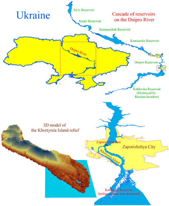
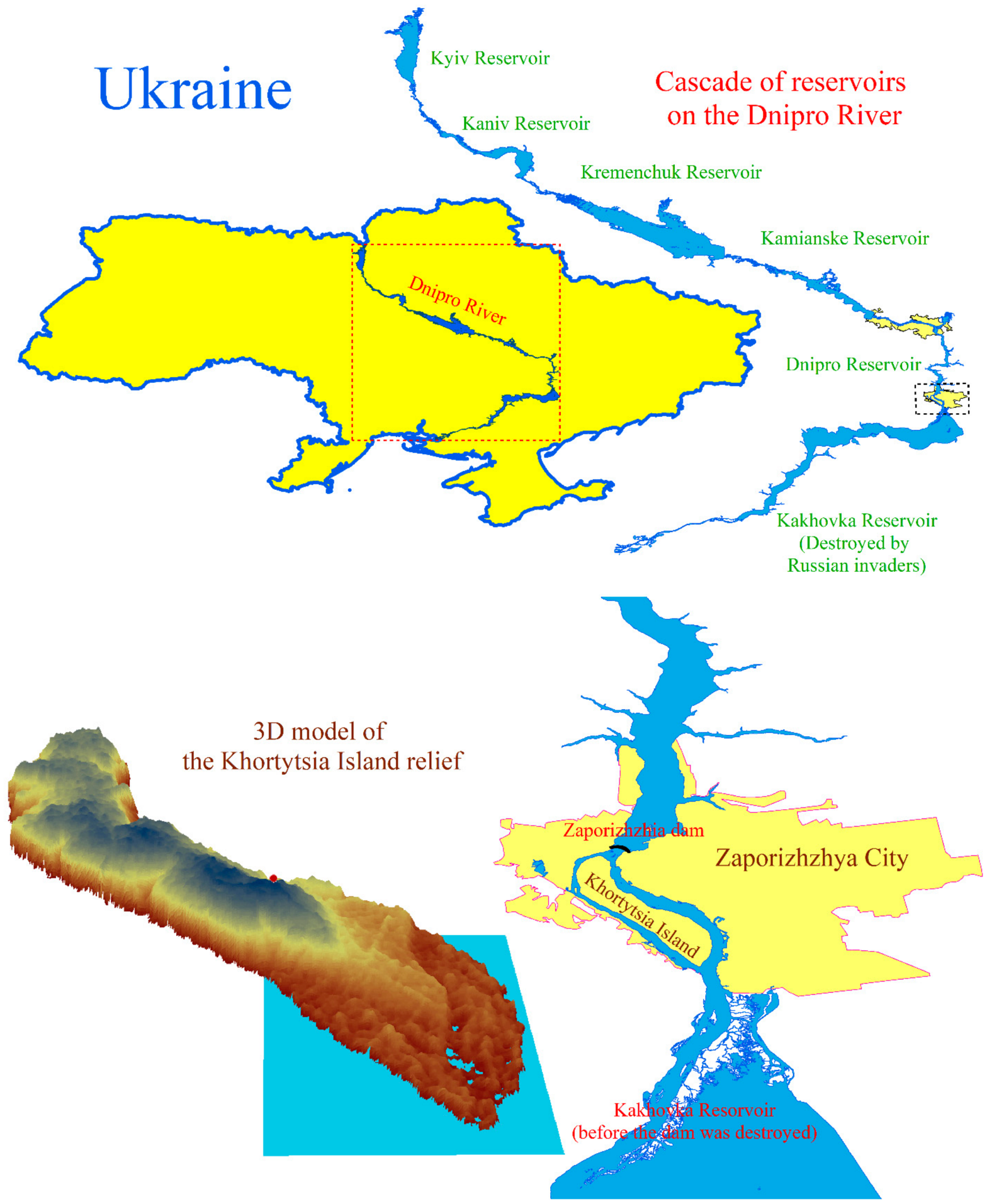
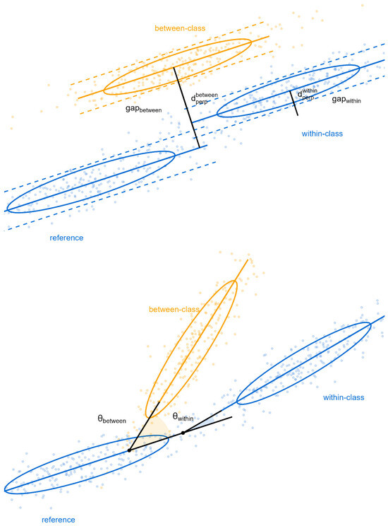
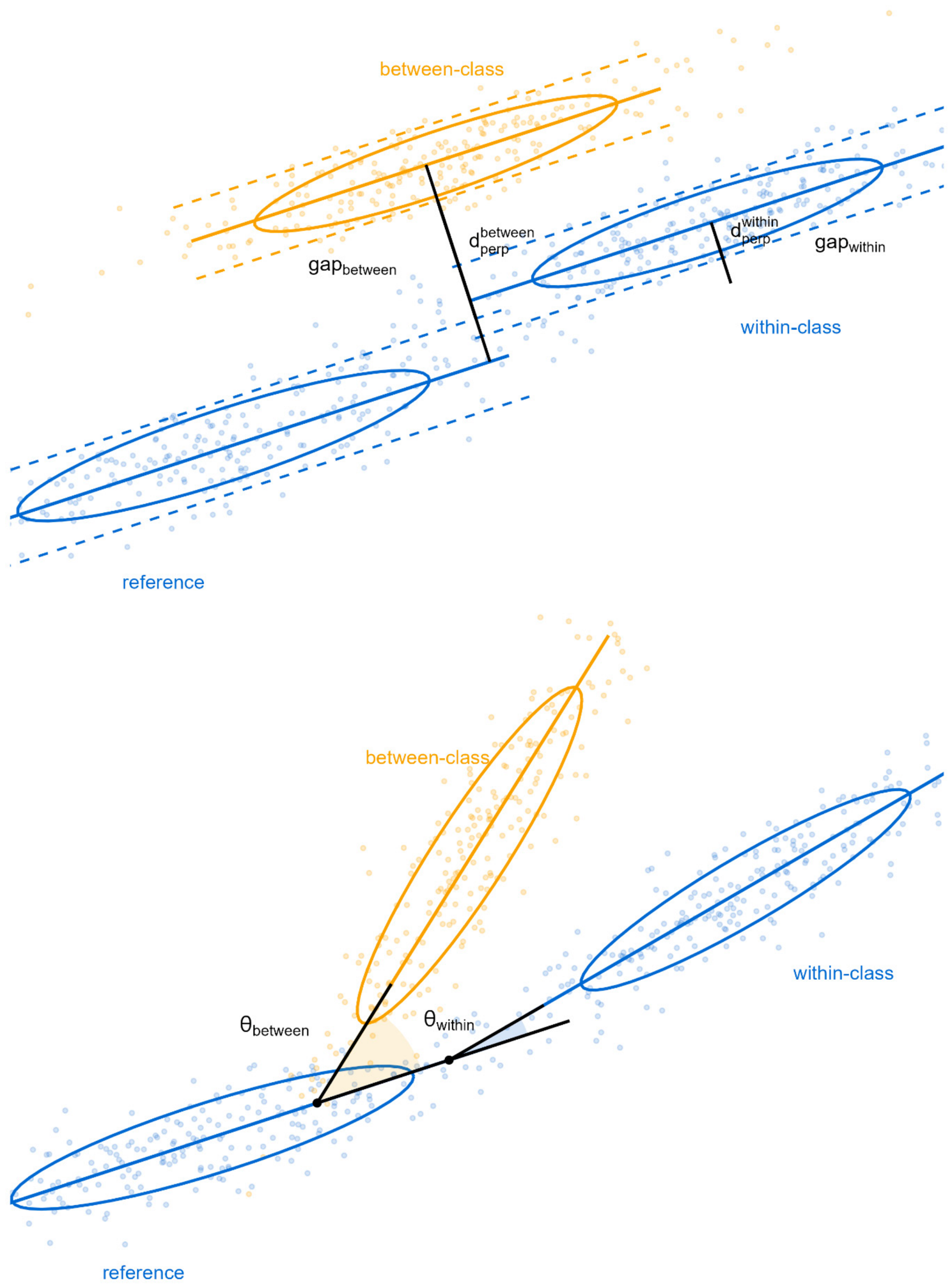
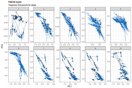
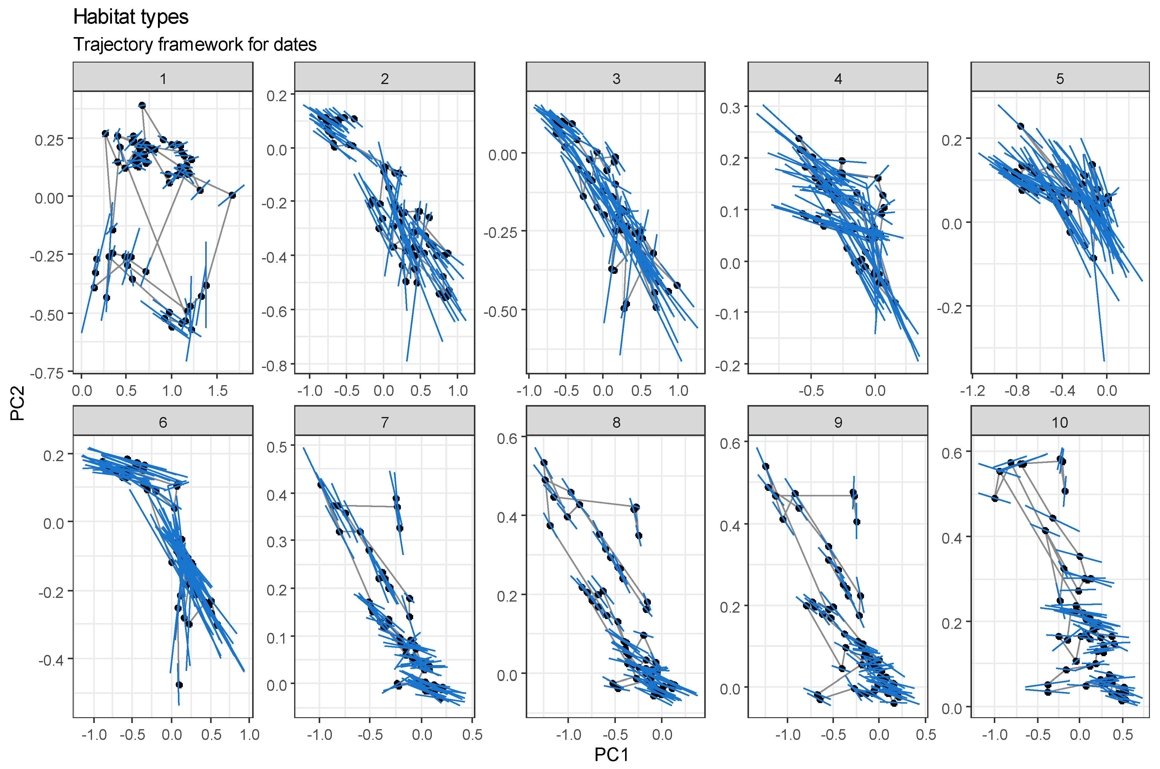
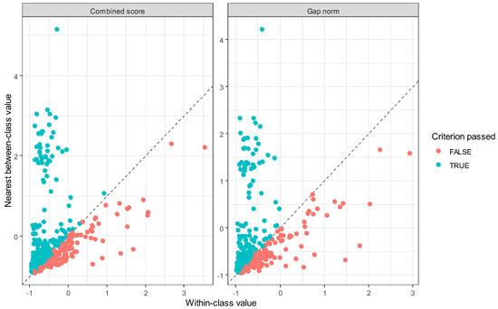
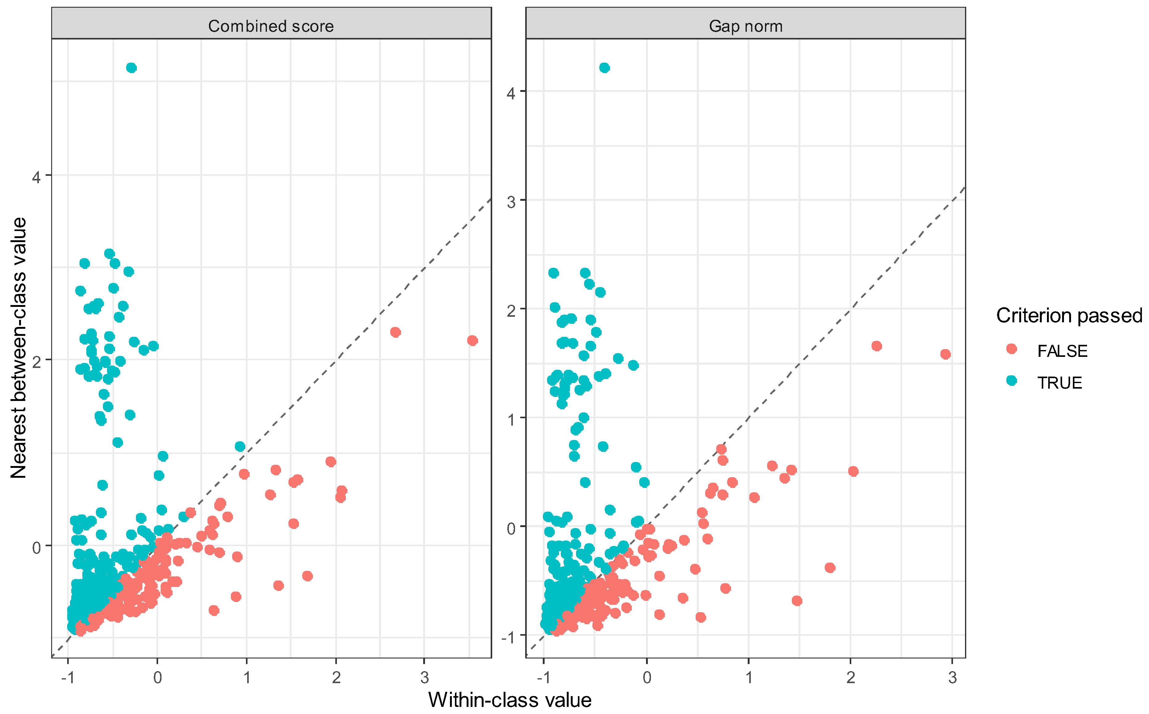
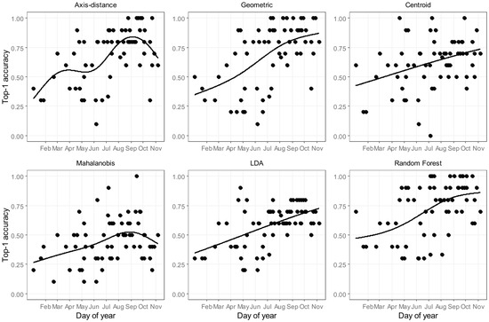
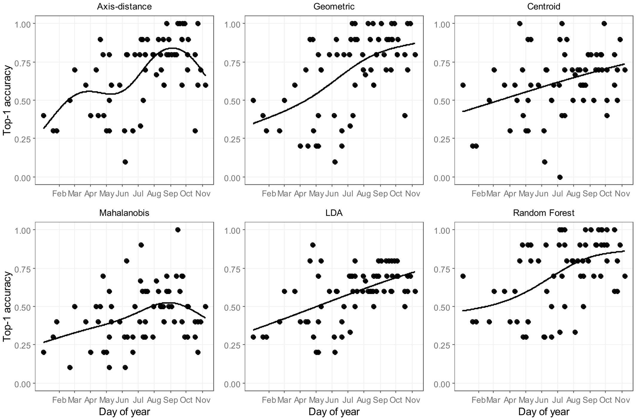
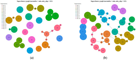
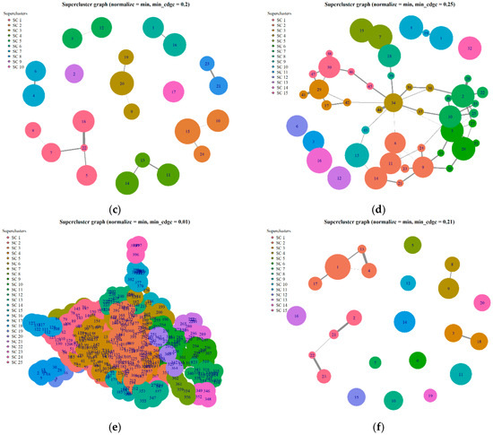
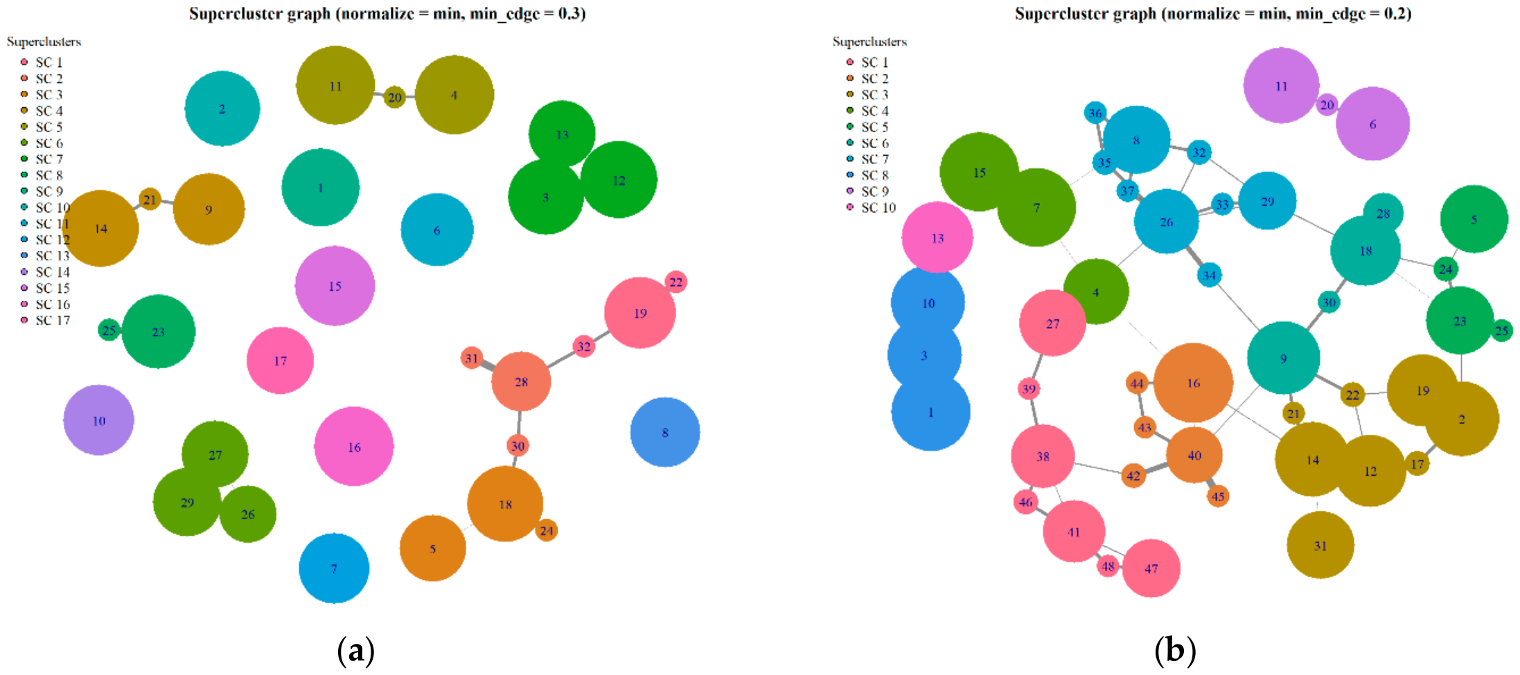
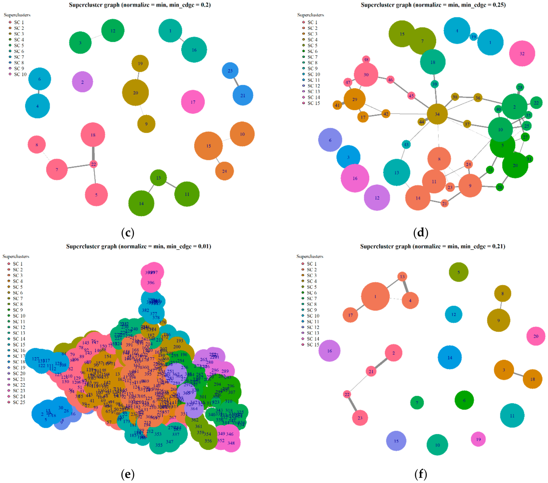
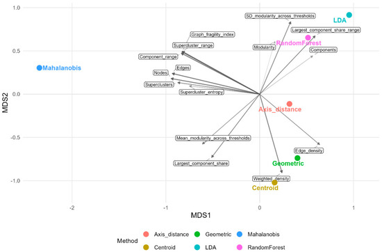
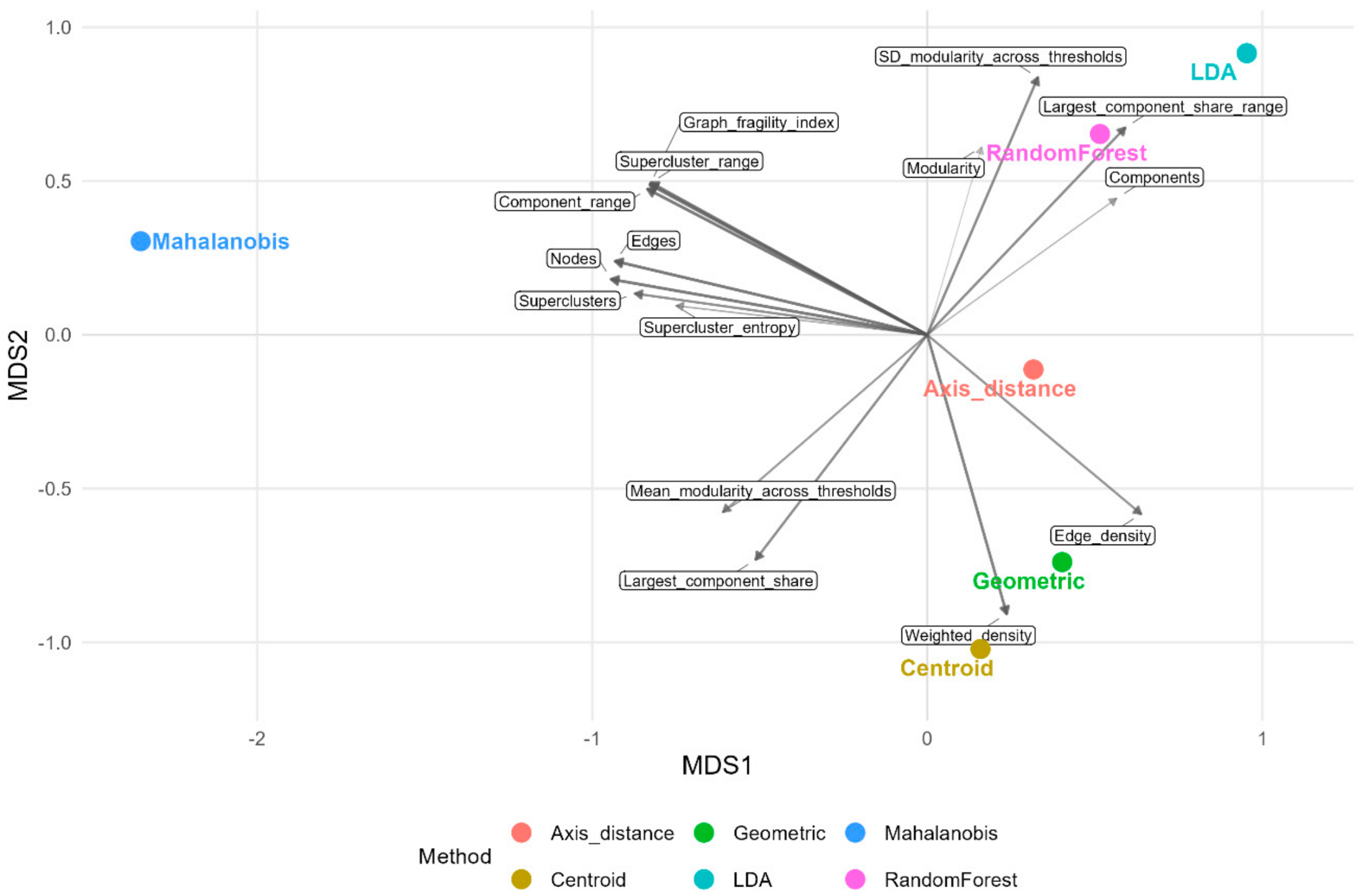
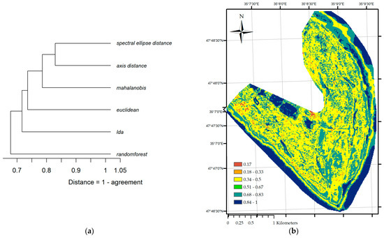
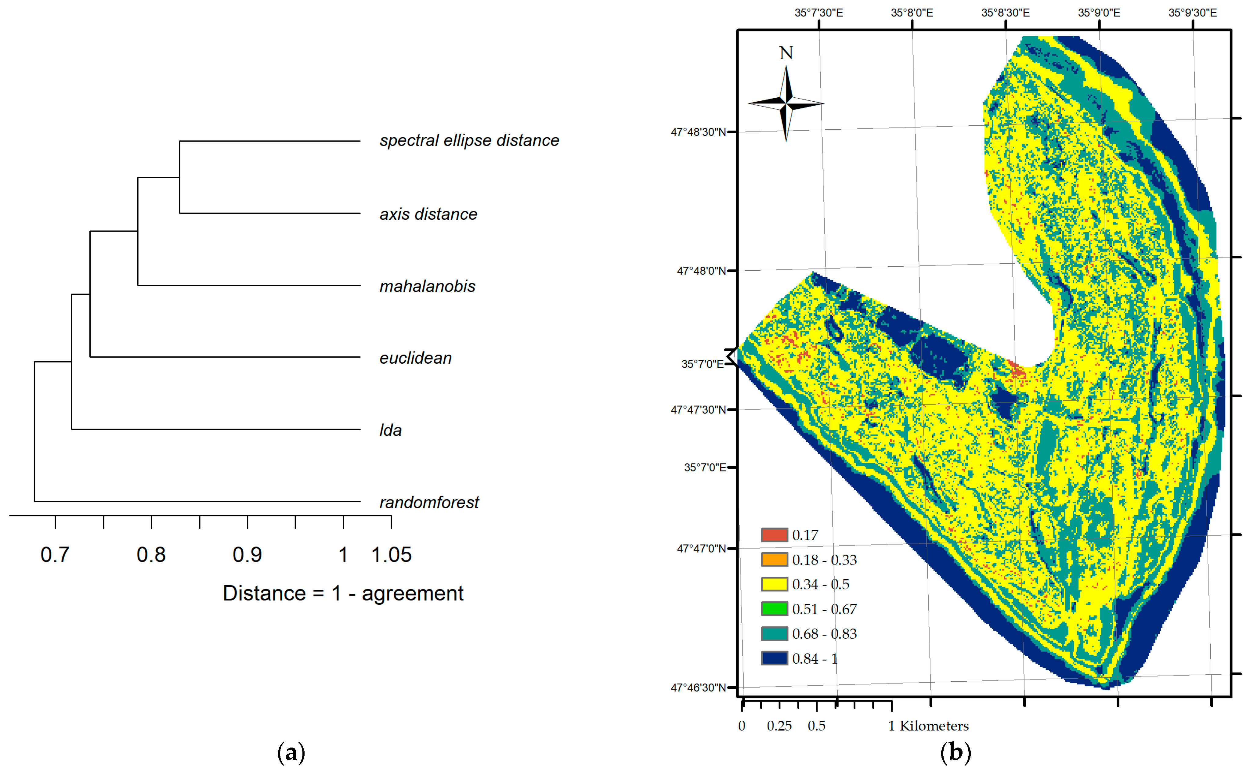
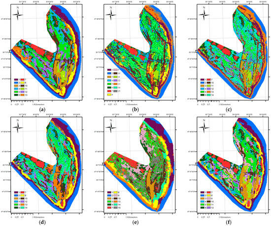
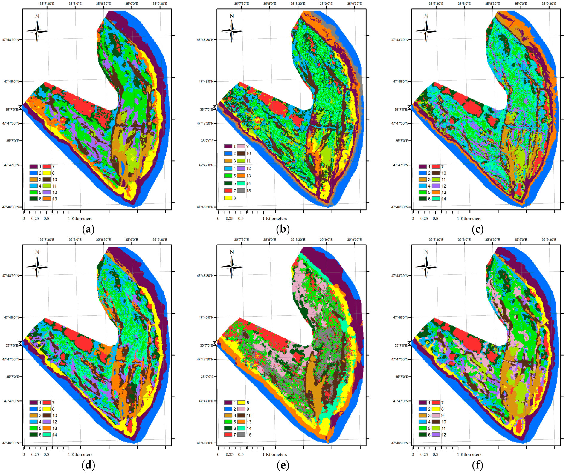

Disclaimer/Publisher’s Note: The statements, opinions and data contained in all publications are solely those of the individual author(s) and contributor(s) and not of MDPI and/or the editor(s). MDPI and/or the editor(s) disclaim responsibility for any injury to people or property resulting from any ideas, methods, instructions or products referred to in the content. |
© 2026 by the authors. Licensee MDPI, Basel, Switzerland. This article is an open access article distributed under the terms and conditions of the Creative Commons Attribution (CC BY) license.